Radiation design in computed tomography via convex optimization
Abstract
Proper X-ray radiation design (via dynamic fluence field modulation, FFM) allows to reduce effective radiation dose in computed tomography without compromising image quality. It takes into account patient anatomy, radiation sensitivity of different organs and tissues, and location of regions of interest. We account all these factors within a general convex optimization framework.
1 Introduction
Recently, there has been significant research interest in dynamic fluence field modulation (FFM), which consists in varying the beam shape throughout the scan allowing for the adaptation of the spatial x-ray distribution to conform to the patient anatomy (cf., e.g., [1] and references therein). A range of hardware solutions have been proposed, including dynamic wedges [2, 3, 4], fluid-filled chambers [5, 6, 7, 8], and slitbased multiple aperture devices [9, 10].
Until now, to the best of our knowledge, the problem of FFM radiation planning has been treated within non-convex optimization framework, and only rough distribution of radiation with relatively small number of parameters (coefficients of basis functions) was modeled. In this work we utilize convex optimization techniques to optimize the fine structure of the fluence, namely, the amount of radiation sent into each projection bin (towards the corresponding detector pixel).111Following the publication of our paper on arXiv, it came to our attention that a concept akin to ours was previously outlined in an unpublished Master’s thesis “Optimal Anisotropic Irradiation For X-Ray Computed Tomography” by Y. Chernyak, Technion, October 2021; see the Technion Graduate School website: https://graduate.technion.ac.il/en/department-en-4msc/
The main body of this paper is organized as follows. In Section 2 we present the CT observation model underlying our derivations, introduce and motivate the loss index of radiation design responsible for the asymptotical, as the total amount of radiation grows, quality of the Maximum Likelihood recovery of the image of interest. We then pose the problem of optimal radiation design as the problem of optimizing the loss index under general convex constraints on the design. The resulting optimization problem is convex and thus efficiently solvable (at least in theory, and to some extent, also in practice). In Section 3, we report on the (in our appreciation, encouraging) results of a “proof of concept” numerical experiment implementing the radiation design proposed in Section 2. Section 4 contains some concluding remarks.
2 CT Radiation Design
2.1 CT observation scheme
The CT observation scheme we intend to consider is as follows:
-
1.
is the “signal” – the discretized body attenuation density, so that is the number of voxels in the field of view;
-
2.
is the vector of observations; observations are indexed by bins, being the total number of bins;
-
3.
is the “projection matrix”;
-
4.
is the vector with entries which are the expected numbers of photons sent to bin during the stude.
We assume that the -th observation stemming from signal is
(1) where is the Poisson distribution with parameter :
We assume also that entries in the vector of observations are independent across .
-
5.
Given observation stemming from the unknown signal , we want to recover the vector , where is a given matrix.222In our experiments is a truncation of image towards the region of interest (ROI). We measure the recovery error in the standard Euclidean norm on .
2.2 Radiation sensitivity - from voxels to bins
Informally, our goal is to find radiation design , which provides best image quality given the whole-body effective dose. Various organs and tissues have different sensitivity to radiation—effective dose caused by unitary radiation exposure. This can be reflected in 3D voxel-wise sensitivity map , which is standardly used in radiation therapy planning.
We assume that, in addition, an (approximate) attenuation map of the body is available, and we can compute an auxiliary bin-sensitivity vector with entries reflecting effective dose obtained from a unit of radiation sent into bin . Constant whole body effective dose is provided by the condition
| (2) |
Thus our goal is to find radiation design , which provides the best image quality under constraint (2).
2.3 Maximum Likelihood estimate
With and given, we intend to recover as , where is the Maximum Likelihood (ML) estimate. Denoting by , , the rows of , the log-likelihood of observing , the signal being , is
Consequently, maximizing in is the same as maximizing in the concave in function
| (3) |
and is therefore an efficiently solvable problem; the resulting estimate
of is a function of depending on as a parameter.
2.4 Radiation Design via Loss index minimization
Our goal is “presumably good,” in terms of the performance of the resulting estimate, selection of in a given compact convex set . This informal goal can be stated formally in different ways; the formalization we propose is based on the following observation.
A. In the “noiseless case” where the observations are , , being the true signal (instead of being Poisson random variables with parameters ), the ML estimate exactly recovers the true signal. In other words, setting , we get . Indeed, since is concave and smooth in , it suffices to verify that , which is evident.
B. Now assume that the positive semidefinite Hessian matrix
is positive definite, or, which is the same when , that is of rank . Let be the second order Taylor approximation of around . Were we specifying our estimate of as
we would have
that is, . Hence, taking into account the immediate relation (recall that are independent across ),
This computation suggests, as a meaningful “loss index” of (the smaller it is, the better for our purposes) the function
| (4) |
Needless to recall, the above reasoning is informal—our estimate of is not , it is . Nevertheless, it can be proved that when is of rank and becomes large, specifically, with , when , our informal reasoning yields correct asymptotics of the expected squared -error of the recovery of 333Namely, with , , one has as .. We, however, neither present these asymptotic results, nor need them—our goal at this point is to find a convenient criterion to be optimized over in order to get a presumably good measurement design, and to this end no rigorous justification of our choice is needed. What indeed is important for us, is that is a convex function of , and thus is well suited for minimization.
A bad news is that strictly speaking, we cannot use as a criterion to be minimized—this quantity depends, as on a parameter, on the unknown to us true signal . On the other hand, when replacing in the right hand side of (4) the unknown quantities with their approximations which are within factor from , that is , the resulting right hand side in (4) is within the same factor from the true one. Therefore, assuming that an approximate attenuation map is available a priori, or that it can be estimated using observation from a pilot run with, say, equal to each other “moderate” , we may select by minimizing over the observable criterion
| (5) |
This is, essentially, the course of actions we propose.
2.5 Regularization
The problem of minimizing over is convex and as such can, theoretically, be solved to whatever high accuracy in a computationally efficient manner. At the same time, numerical experimentation shows that this problem may happen to be ill-conditioned, resulting in difficulties when solving it numerically. To overcome, to some extent, these difficulties, we can replace minimizing over the objective given by (5) with minimizing over the same domain the penalized objective
| (6) |
where regularizing coefficient is nonnegative; a good value of this coefficient could be found experimentally. Thus, in the sequel we intend to optimize measurement design by solving convex optimization problem
| (7) |
which can be solved by standard Convex Optimization algorithms. It turns out, however, that one can utilize problem’s structure to design a dedicated algorithm which, as our experiments show, is much faster than the “general purpose” algorithms. The following underlying observation is essentially well known:
Proposition 1.
Let be an matrix of rank , be a matrix, and be positive -dimensional vectors. Then, setting ,
| (8a) | |||||
| (8b) | |||||
where is the Frobenius norm
Alternating minimization.
Proposition 1 suggests the alternating minimization algorithm for minimizing over . Assume for the sake of definiteness that (modification for the case of is immediate). By (8a), the problem of interest (7) can be rewritten equivalently as
To solve the latter problem, we start with some positive . At a step of the algorithm, given positive ,
-
•
we minimize over ; this is an unconstrained minimization problem with strongly convex quadratic objective, and its solution is given by explicit formula:
(9) -
•
after is computed, we specify by minimizing over , which boils down to finding
When is simple, the latter problem is simple as well. For instance, in the case of with , assuming that has no zero columns (which can be ensured by an arbitrarily small perturbation of , the solution is given by
(10)
After are computed, we pass to step .
3 Computational experiment

Here we report on a toy “proof of concept” numerical experiment on recovering -pixel Shepp-Logan type phantom with 68 projection angles spread uniformly over 360 degrees.
3.1 Experimental setup
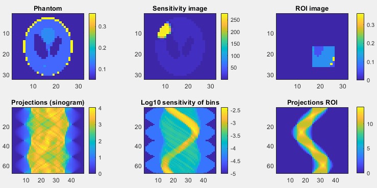
Unlike conventional tomography, where 180 degree angle span is sufficient, we consider 360 degree span to account for the fact that effective radiation dose is generally different when photons are sent along the same line from opposite directions due to different attenuation between the source and a particular body point. In our experiments, the number of bins is ; we utilize the baseline (uniform) radiation design e5 photons/bin. Figure 1, top row, shows the attenuation map, radiation sensitivity, and region of interest (ROI) which we aim to reconstruct. Bottom row shows the corresponding maps in the sinogram (projection) space.444When computing sinograms we used a partially modified “Matlab demo for 2-D tomographic reconstruction” toolbox by L. Han, see https://github.com/phymhan/matlab-tomo-2d. In particular, the middle picture shows radiation sensitivity in projection space, i.e. effective dose caused by a unit of radiation sent into each projection bin. One can see a bright curve strip of high sensitivity. As we will see later, our algorithm will reduce amount of radiation sent into this strip.
Building the field design vector in the model presented in the previous section requires, along with the matrices and readily given by the geometry of bins and the ROI, the knowledge of vectors and with entries indexed by bins. The entries in are proportional to our guess on effective dose from a single photon sent into the corresponding bin, and entries in are estimations of the quantities . Both these vectors depend on the actual image . “In real life” they may be either considered available a priori or should be obtained from a pilot recovery of in which the radiation is a small fraction of split, say, equally between bins. In our “proof of concept” experiment where the goal is to understand potential of radiation design we use “ideal” values of and ; in particular, we set . To specify we act as follows: first, we utilize and pixel sensitivities image depicted in Figure 1 to compute the effective dose caused by a single photon sent through the bin . Then, to get , we scale to ensure that , where is the uniform (“baseline”) design such that the radiation in every bin is .
3.2 Computations
Design optimization was carried out using alternating minimization (9)–(10) described in Section 2.5; 5-6 iterations of the process turned out to be sufficient to get high accuracy solution. An alternative, somehow more time consuming solution is provided by the first order algorithm—Mirror Descent with simplex setup, see [11, Lecture 5]. Maximum Likelihood estimate was computed utilizing Nesterov’s Fast Gradients [12] for minimizing smooth convex functions over the nonnegative orthant.
3.3 Numerical results
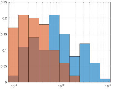
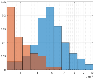
We present results of two experiments for the phantom image presented in Figure 1 and two values of the regularization parameter, and e. Figure 2 shows the obtained optimized radiation design in the penalized problem. The optimization results in significant reduction of radiation in the sensitive area and its increase in the ROI-related part of the sinogram.

In each experiment we compute recoveries utilizing baseline and optimized designs; in Figure 3 we present the histograms of the mean square error (MSE—squared recovery error per ROI pixel).
 |
 |
Figure 4 shows typical recoveries of the ROI image in the case of . One can observe a clear image quality improvement under the optimized design.

4 Concluding remarks
We present the first attempt to treat CT radiation design within a convex optimization framework. Unlike conventional design, it takes into account the radiation sensitivity map of the body, therefore minimizing the total effective dose.
Further challenges and opportunities
3D reconstruction
In the 3D case the number of voxels scales as with single-dimension grid size, while the number of bins grows as . This gives much more degrees of freedom for the optimal design than in the 2D case. On the other hand, a faster algorithm is needed to implement radiation design in a reasonable time.
Our approach is especially attractive for use in radiation therapy rooms, where a preliminary radiation sensitivity map of a patient is readily available. It may be used e.g. with kilo-voltage cone-beam CT (kV-CBCT) systems integrated into the gantry of linear accelerators. [13, 14].
One more point to note: usually cone beam CT gantry moves with maximal axial speed so that each body point is exposed to x-ray only once for a given transaxial angle. It may be better to slow this movement down, allowing multiple axial x-ray angles for each tranaxial angle. This would improve the reconstruction noise-to-dose ratio in CT systems in both cases, with and without control of radiation pattern.
Radiation design under constraints
In this work the design is optimized using an asymptotic maximum likelihood reconstruction model under unique effective dose constraint (2). One can easily impose extra convex constraints on the radiation vector (e.g., total radiation dose, maximal dose per pixel, etc). Furthermore, the proposed design optimization framework can be adapted to account for the available a priori information about the body image when it is formulated in the form of convex constraints on the image space (cf., e.g., [15, Section 6.4.2]).
Appendix A Proof of Proposition 1
Given matrix of rank and , consider the optimization problem
The objective in this unconstrained minimization problem is a strongly convex quadratic function, so that optimal is given the unique solution to the Fermat equation
resulting in
where the second equality is due to Sherman-Morrison formula. Direct computation shows that for this one has
Setting and substituting the optimization variable with , we arrive at (8a). Passing in the latter relation to limit as and taking into account that is of rank , we arrive at (8b). ∎
References
- [1] G. J. Gang, J. H. Siewerdsen, and J. W. Stayman, “Task-driven optimization of fluence field and regularization for model-based iterative reconstruction in computed tomography,” IEEE transactions on medical imaging, vol. 36, no. 12, pp. 2424–2435, 2017.
- [2] T. P. Szczykutowicz and C. A. Mistretta, “Design of a digital beam attenuation system for computed tomography: Part i. system design and simulation framework,” Medical physics, vol. 40, no. 2, p. 021905, 2013.
- [3] S. S. Hsieh and N. J. Pelc, “The feasibility of a piecewise-linear dynamic bowtie filter,” Medical physics, vol. 40, no. 3, p. 031910, 2013.
- [4] F. Liu, G. Wang, W. Cong, S. S. Hsieh, and N. J. Pelc, “Dynamic bowtie for fan-beam ct,” Journal of X-ray Science and Technology, vol. 21, no. 4, pp. 579–590, 2013.
- [5] W. Peppler, B. Kudva, J. Dobbins III, C. Lee, M. Van Lysel, B. Hasegawa, and C. Mistretta, “Digitally controlled beam attenuator,” in Application of Optical Instrumentation in Medicine X, vol. 347, pp. 106–111, SPIE, 1982.
- [6] T. P. Szczykutowicz and J. Hermus, “Fluid dynamic bowtie attenuators,” in Medical Imaging 2015: Physics of Medical Imaging, vol. 9412, pp. 219–225, SPIE, 2015.
- [7] P. Shunhavanich, S. S. Hsieh, and N. J. Pelc, “Fluid-filled dynamic bowtie filter: a feasibility study,” in Medical Imaging 2015: Physics of Medical Imaging, vol. 9412, pp. 399–406, SPIE, 2015.
- [8] F. Liu, Q. Yang, W. Cong, and G. Wang, “Dynamic bowtie filter for cone-beam/multi-slice ct,” PloS one, vol. 9, no. 7, p. e103054, 2014.
- [9] J. W. Stayman, A. Mathews, W. Zbijewski, G. Gang, J. Siewerdsen, S. Kawamoto, I. Blevis, and R. Levinson, “Fluence-field modulated x-ray ct using multiple aperture devices,” in Medical Imaging 2016: Physics of Medical Imaging, vol. 9783, pp. 232–237, SPIE, 2016.
- [10] A. Mathews, G. Gang, R. Levinson, W. Zbijewski, S. Kawamoto, J. Siewerdsen, and J. Stayman, “Experimental evaluation of dual multiple aperture devices for fluence field modulated x-ray computed tomography,” in Medical Imaging 2017: Physics of Medical Imaging, vol. 10132, pp. 690–695, SPIE, 2017.
- [11] A. Ben-Tal and A. Nemirovski, “Lectures on modern convex optimization (2020),” SIAM, Philadelphia, PA. Google Scholar Google Scholar Digital Library Digital Library, 2021.
- [12] Y. Nesterov, Lectures on convex optimization, vol. 137. Springer, 2018.
- [13] K. Srinivasan, M. Mohammadi, and J. Shepherd, “Applications of linac-mounted kilovoltage cone-beam computed tomography in modern radiation therapy: A review,” Polish journal of radiology, vol. 79, p. 181, 2014.
- [14] J. Wang, T. Li, Z. Liang, and L. Xing, “Dose reduction for kilovotage cone-beam computed tomography in radiation therapy,” Physics in Medicine & Biology, vol. 53, no. 11, p. 2897, 2008.
- [15] A. Juditsky and A. Nemirovski, Statistical Inference via Convex Optimization. Princeton University Press, 2020.