Learning Optimal Phase-Shifts of Holographic Metasurface Transceivers

Debamita Ghosh, IITB-Monash Research Academy, IIT Bombay, India
Manjesh K. Hanawal, MLioNS Lab, IEOR, IIT Bombay, India
Nikola Zlatanov, Innopolis University, Russia
Abstract

Holographic metasurface transceivers (HMT) is an emerging technology for enhancing the coverage and rate of wireless communication systems. However, acquiring accurate channel state information in HMT-assisted wireless communication systems is critical for achieving these goals. In this paper, we propose an algorithm for learning the optimal phase-shifts at a HMT for the far-field channel model. Our proposed algorithm exploits the structure of the channel gains in the far-field regions and learns the optimal phase-shifts in presence of noise in the received signals. We prove that the probability that the optimal phase-shifts estimated by our proposed algorithm deviate from the true values decays exponentially in the number of pilot signals. Extensive numerical simulations validate the theoretical guarantees and also demonstrate significant gains as compared to the state-of-the-art policies.

Index Terms:
Holographic Metasurface Transceivers, Channel State Information, Uniform Exploration

I Introduction

Future wireless network technologies, namely beyond-5G and 6G, have been focused on millimeter wave (mmWave) and TeraHertz (THz) communications technologies as possible solutions to the ever growing demands for higher data rates and lower latency. However, mmWave and THz communications have challenges that need to be addressed before this technology is adopted [1], [2]. One such major challenge is signal deterioration due to reflections and absorption.

A possible solution for the signal deterioration are base stations (BSs) with massive antennas arrays that can provide large beamforming gains and thereby compensate for the signal deterioration [3]. However, implementing a BS with a massive antenna array is itself challenging due to the high hardware costs. Holographic Metasurface Transceivers (HMTs) are introduced as a promising solution for building a massive antenna array [4, 5]. A HMT is comprised of a large number of metamaterial elements densely deployed into a limited surface area in order to form a spatially continuous transceiver aperture. These metamaterial elements at the HMT acts as phase-shifting antennas, where each phase-shifting element of the HMT can change the phase of transmiting/receiving signal and thereby beamform towards desired directions where the users are allocated [6]. Due to these continuous apertures, HMTs can be represented as an extension of the traditional massive antenna arrays with discrete antennas to continuous reflecting surfaces [6].

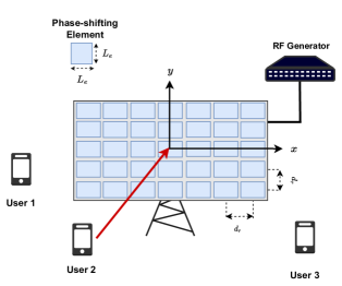
In this paper, we consider the HMT-assisted wireless systems illustrated in Fig. 1, where a HMT acts as a BS that serves multiple users. The performance of this system is dependent on channel state information (CSI) estimates at the HMT, which are used for accurate beamforming towards the users. The authors in [7] and [8] have studied the effect of HMT-assisted systems on enhancing the communication performance under the assumption of perfect CSI. However, perfect CSI is not available in practice. In practice, the CSI has to be estimated via pilot signals, which results in inaccurate CSI estimates at the HMT.

The aim of this paper is to obtain accurate CSI estimates at the HMT, which in turn is used to set the optimal phase-shifts at the HMT that maximize the data rate to the users when the users are located in the far-field. To this end, we exploit the structure of the far-field channel model between the HMT and the users to show that the optimal phase-shifts at the HMT can be obtained from five samples of the received pilot signals at the HMT in a noiseless environment. We then use this approach to develop a learning algorithm that learns the optimal phase-shifts from the received pilot signals at the HMT in a noisy environment. Finally, we provide theoretical guarantees for our learning algorithm. Specifically, we prove that the probability of the phase-shifts generated by our algorithm to deviate by more than ϵitalic-ϵ\epsilon from the optimal phase-shifts is small and decays as the number of pilot symbols increases. The error analysis is based on tail probabilities of the non-central Chi-squared distribution.

In summary, our main contributions are as follows:

  • We propose an efficient learning algorithm for estimating the optimal phase-shifts at an HMT in the presence of noise for the case when the users that the HMT is serving are located at the far-field region.

  • We prove that the probability of the phase-shifts generated by our algorithm to deviate by more than ϵitalic-ϵ\epsilon from the optimal phase-shifts is small and decays exponentially as the number of pilots used for estimation increases.

  • We show numerically that the performance of the proposed algorithm significantly outperforms existing CSI estimation algorithms.

I-A Related Works

Several channel estimation schemes, which are proposed for the massive antenna arrays, are also applicable to the considered HMT including exhaustive search [9], hierarchical search [10], [11], and compressed sensing (CS) [11]. As the exhaustive search in [9] significantly increases the training overhead, the authors in [10] and [11] proposed the hierarchical search based on a predefined codebook as an improvement over the exhaustive search. The hierarchical schemes, in general, may incur high training overhead and system latency since they require non-trivial coordination among the transmitter and the user [11]. On the other hand, the proposed CS-based channel estimation scheme in [11] provides trade-offs between accuracy of estimation and training overhead at different computational costs.

On the other hand, CSI estimation schemes developed specifically for HMTs can be found in [12] and [13]. The authors in [12] proposed the least-square estimation based approach to study the channel estimation problem for the uplink between a single user and the BS equipped with the holographic surface with a large number of antennas. However, the authors require an additional knowledge of antennas array geometry to reduce the pilot overhead required by the channel estimation, and hence the computational complexity scales up with the number of antennas at the BS. In [13], the authors proposed a scheme for the estimation of the far-field channel between a HMT and a user that requires only five pilots for perfect estimation in the noise-free environment. In the noisy case, the authors of [13] proposed an iterative algorithm that efficiently estimates the far-field channel. Unlike the existing works, the training overhead and the computational cost of the proposed scheme in [13] does not scale with the number of phase-shifting elements at the HMT. The iterative algorithm in [13] significantly outperforms the hierarchical and CS based schemes. However, the authors in [13] did not provide any theoretical guarantees on their proposed algorithm. Motivated by [13], in this work, we propose an algorithm which outperforms the one in [13], and, in addition, we also provide theoretical guarantees for our proposed algorithm.

This paper is organized as follows. The system and channel models for the HMT communication system are given in Sec. II. The proposed algorithm for learning the optimal phase-shifts is given in Sec. III and its theoretical guarantee is provided in Sec. IV. Numerical evaluation of the proposed algorithm is provided in Sec. V. Finally, Sec. VI concludes the paper.

II System and Channel Models

We consider a HMT-assisted wireless communication system, shown in Fig. 1, where an HMT communicates with multiple users in the mmWave band. We assume that there is a Line of Sight (LoS) between the HMT and each user. As a result, when modeling the far-field channel, we only take into account the LoS path since its power is order of magnitude higher than non-line-of-sight (NLoS) paths [14]. The NLoS components are incorporated in the noise. We assume that the users send orthogonal pilots to the HMT for channel estimation. Based on the estimated CSI at the HMT to each user, the HMT sends data to the users. Hence, the data rate from the HMT to the users is directly dependent on the accuracy of the CSI estimates at the HMT. Since in this paper our main goal is the accurate CSI estimation at the HMT to each user, which in turn send orthogonal pilots to the HMT, in the rest of the paper, we will focus on the CSI estimation between the HMT and a typical user.
Refer to caption
Figure 1: The HMT-assisted wireless communication system [13].

II-A HMT Model

The HMT has a rectangular surface of size Lx×Lysubscript𝐿𝑥subscript𝐿𝑦L_{x}\times L_{y}, where Lxsubscript𝐿𝑥L_{x} and Lysubscript𝐿𝑦L_{y} are the width and the length of the surface, respectively. The HMT’s surface is comprised of a large number of sub-wavelength phase-shifting elements, where each elements is assumed to be a square of size Le×Lesubscript𝐿𝑒subscript𝐿𝑒L_{e}\times L_{e} and can change the phase of the transmit/receive signal independently from rest of the elements. Let drsubscript𝑑𝑟d_{r} be the distance between two neighboring phase-shifting elements. The total number of phase-shifting elements of the HMT is given by M=Mx×My𝑀subscript𝑀𝑥subscript𝑀𝑦M=M_{x}\times M_{y}, where Mx=Lx/drsubscript𝑀𝑥subscript𝐿𝑥subscript𝑑𝑟M_{x}=L_{x}/d_{r} and My=Ly/drsubscript𝑀𝑦subscript𝐿𝑦subscript𝑑𝑟M_{y}=L_{y}/d_{r}. Without loss of generality, we assume that the HMT lies in the xy𝑥𝑦x-y plane of a Cartesian coordinate system, where the center of the surface is at the origin of the coordinate system. Assuming Mxsubscript𝑀𝑥M_{x} and Mysubscript𝑀𝑦M_{y} are odd numbers, the position of the (mx,my)thsuperscriptsubscript𝑚𝑥subscript𝑚𝑦𝑡(m_{x},m_{y})^{th} phase-shifting element in the Cartesian coordinate system is given as (x,y)=(mxdr,mydr),𝑥𝑦subscript𝑚𝑥subscript𝑑𝑟subscript𝑚𝑦subscript𝑑𝑟(x,y)=(m_{x}d_{r},m_{y}d_{r}), where mx{Mx12,,Mx12}subscript𝑚𝑥subscript𝑀𝑥12subscript𝑀𝑥12m_{x}\in\left\{-\frac{M_{x}-1}{2},\dots,\frac{M_{x}-1}{2}\right\} and my{My12,,My12}subscript𝑚𝑦subscript𝑀𝑦12subscript𝑀𝑦12m_{y}\in\left\{-\frac{M_{y}-1}{2},\dots,\frac{M_{y}-1}{2}\right\}. When Mxsubscript𝑀𝑥M_{x} or Mysubscript𝑀𝑦M_{y} is even, the position of the (mx,my)thsuperscriptsubscript𝑚𝑥subscript𝑚𝑦𝑡(m_{x},m_{y})^{th} element can be appropriately defined.

II-B Channel Model

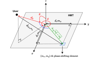
Consider the channel between the (mx,my)thsuperscriptsubscript𝑚𝑥subscript𝑚𝑦𝑡(m_{x},m_{y})^{th} phase-shifting element at the HMT and the typical user. Let the beamforming weight imposed by the (mx,my)thsuperscriptsubscript𝑚𝑥subscript𝑚𝑦𝑡(m_{x},m_{y})^{th} phase-shifting element at the HMT be Γmxmy=ejβmxmysubscriptΓsubscript𝑚𝑥subscript𝑚𝑦superscript𝑒𝑗subscript𝛽subscript𝑚𝑥subscript𝑚𝑦\Gamma_{m_{x}m_{y}}=e^{j\beta_{m_{x}m_{y}}}, where βmxmysubscript𝛽subscript𝑚𝑥subscript𝑚𝑦\beta_{m_{x}m_{y}} is the phase shift at the (mx,my)thsuperscriptsubscript𝑚𝑥subscript𝑚𝑦𝑡(m_{x},m_{y})^{th} element. Let λ𝜆\lambda denote the wavelength of the carrier frequency, k0=2πλsubscript𝑘02𝜋𝜆k_{0}=\frac{2\pi}{\lambda} be the wave number, d0subscript𝑑0d_{0} be the distance between the user and the center of the HMT and let Fmxmysubscript𝐹subscript𝑚𝑥subscript𝑚𝑦F_{m_{x}m_{y}} denote the effect of the size and power radiation pattern of the (mx,my)thsuperscriptsubscript𝑚𝑥subscript𝑚𝑦𝑡(m_{x},m_{y})^{th} phase-shifting element on the channel coefficient [15]. Due to the far-field assumptions, the radiation pattern of all the phase-shifting elements of the HMT are identical, i.e., Fmxmy=F,mx,mysubscript𝐹subscript𝑚𝑥subscript𝑚𝑦𝐹for-allsubscript𝑚𝑥subscript𝑚𝑦F_{m_{x}m_{y}}=F,\;\forall m_{x},m_{y} holds. Finally, let θ𝜃\theta and ϕitalic-ϕ\phi denote the elevation and azimuth angles of the impinging wave from the user to the center of the HMT, see Fig. 2.
Refer to caption
Figure 2: Distance between the (mx,my)subscript𝑚𝑥subscript𝑚𝑦(m_{x},m_{y})-th phase-shifting element at the HMT and the user [13].

Now, if the phase-shift imposed by the (mx,my)thsuperscriptsubscript𝑚𝑥subscript𝑚𝑦𝑡(m_{x},m_{y})^{th} element, βmx,mysubscript𝛽subscript𝑚𝑥subscript𝑚𝑦\beta_{m_{x},m_{y}}, is set to

βmxmy=mod(k0dr(mxβ1+myβ2),2π),mx,my,\beta_{m_{x}m_{y}}=-\mod(k_{0}d_{r}(m_{x}\beta_{1}+m_{y}\beta_{2}),2\pi),\forall m_{x},m_{y},

where β1subscript𝛽1\beta_{1} and β2subscript𝛽2\beta_{2} are the phase-shift parameters [13], [16], [17], which are the only degrees of freedom within the phase-shift βmxmysubscript𝛽subscript𝑚𝑥subscript𝑚𝑦\beta_{m_{x}m_{y}}, then the HMT-user channel in the far-field is approximated accurately by [13], [16], [17]

H(β1,β2)𝐻subscript𝛽1subscript𝛽2\displaystyle H(\beta_{1},\beta_{2}) =(Fλejk0d04πd0)LxLy×sinc(Kxπ(α1β1))absent𝐹𝜆superscript𝑒𝑗subscript𝑘0subscript𝑑04𝜋subscript𝑑0subscript𝐿𝑥subscript𝐿𝑦sincsubscript𝐾𝑥𝜋subscript𝛼1subscript𝛽1\displaystyle=\left(\frac{\sqrt{F}\lambda e^{-jk_{0}d_{0}}}{4\pi d_{0}}\right)L_{x}L_{y}\times\mathrm{sinc}\bigg{(}K_{x}\pi(\alpha_{1}-\beta_{1})\bigg{)}
×sinc(Kyπ(α2β2)),absentsincsubscript𝐾𝑦𝜋subscript𝛼2subscript𝛽2\displaystyle\qquad\qquad\times\mathrm{sinc}\bigg{(}K_{y}\pi(\alpha_{2}-\beta_{2})\bigg{)}, (1)

where Kx=Lxλ,Ky=Lyλ,α1=sin(θ)cos(ϕ),α2=sin(θ)sin(ϕ),formulae-sequencesubscript𝐾𝑥subscript𝐿𝑥𝜆formulae-sequencesubscript𝐾𝑦subscript𝐿𝑦𝜆formulae-sequencesubscript𝛼1𝜃italic-ϕsubscript𝛼2𝜃italic-ϕK_{x}=\frac{L_{x}}{\lambda},K_{y}=\frac{L_{y}}{\lambda},\alpha_{1}=\sin(\theta)\cos(\phi),\alpha_{2}=\sin(\theta)\sin(\phi), and sinc(x)=sin(x)xsinc𝑥𝑥𝑥\mathrm{sinc}(x)=\frac{\sin(x)}{x}. Please note that α1[1,1]subscript𝛼111\alpha_{1}\in[-1,1] and α2[1,1]subscript𝛼211\alpha_{2}\in[-1,1], and their values depend on the location of the user, i.e., on θ𝜃\theta and ϕitalic-ϕ\phi.

From (1), it is clear that the absolute value of the HMT-user channel is maximized when the two sinc functions attain their maximum values, which occurs when the phase-shifting parameters, β1subscript𝛽1\beta_{1} and β2subscript𝛽2\beta_{2}, are set to β1=α1subscript𝛽1subscript𝛼1\beta_{1}=\alpha_{1} and β2=α2subscript𝛽2subscript𝛼2\beta_{2}=\alpha_{2}, where (α1,α2)subscript𝛼1subscript𝛼2(\alpha_{1},\alpha_{2}) are unknown to the HMT since they depend on the location of the user. Therefore, in the far-field case, the problem of finding the optimal phase-shifts of the elements at the HMT reduces to estimating the two parameters, α1subscript𝛼1\alpha_{1} and α2subscript𝛼2\alpha_{2} at the HMT.

Remark 1.

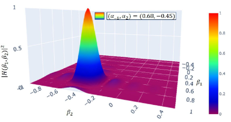
Fig. 3 shows an example of |H(β1,β2)|𝐻subscript𝛽1subscript𝛽2|H(\beta_{1},\beta_{2})| as a function of (β1,β2)subscript𝛽1subscript𝛽2(\beta_{1},\beta_{2}). As can be seen from Fig. 3, the graph of |H(β1,β2)|𝐻subscript𝛽1subscript𝛽2|H(\beta_{1},\beta_{2})| hits zero periodically and has several lobes. The optimal value (α1,α2)=(0.68,0.45)subscript𝛼1subscript𝛼20.680.45(\alpha_{1},\alpha_{2})=(0.68,-0.45) is attained at the central lobe which has the highest peak and is attained for (β1,β2)=(α1,α2)=(0.68,0.45).subscriptsuperscript𝛽1subscriptsuperscript𝛽2subscript𝛼1subscript𝛼20.680.45(\beta^{*}_{1},\beta^{*}_{2})=(\alpha_{1},\alpha_{2})=(0.68,-0.45).

Refer to caption
Figure 3: |H(β1,β2)|𝐻subscript𝛽1subscript𝛽2|H(\beta_{1},\beta_{2})| v/s (β1,β2)subscript𝛽1subscript𝛽2(\beta_{1},\beta_{2}) for values of (α1,α2)=(0.68,0.45).subscript𝛼1subscript𝛼20.680.45(\alpha_{1},\alpha_{2})=(0.68,-0.45).

III Proposed Channel Estimation Strategy

In this section, we propose an algorithm that estimates the optimal phase-shifting parameters β1subscript𝛽1\beta_{1} and β2subscript𝛽2\beta_{2} that maximize |H(β1,β2)|𝐻subscript𝛽1subscript𝛽2\left\lvert H(\beta_{1},\beta_{2})\right\rvert in (1) in the presence of noise.

III-A Problem Formulation

In the channel estimation procedure, the user sends a pilot symbol xp=Psubscript𝑥𝑝𝑃x_{p}=\sqrt{P} to the HMT, where P𝑃P is the pilot transmit power. Then, the received signal at the HMT for fixed phase-shifting parameters (β1,β2),subscript𝛽1subscript𝛽2(\beta_{1},\beta_{2}), denoted by y(β1,β2)𝑦subscript𝛽1subscript𝛽2y(\beta_{1},\beta_{2}), is given by

y(β1,β2)𝑦subscript𝛽1subscript𝛽2\displaystyle y(\beta_{1},\beta_{2}) =P×H(β1,β2)+ζ,absent𝑃𝐻subscript𝛽1subscript𝛽2𝜁\displaystyle=\sqrt{P}\times H(\beta_{1},\beta_{2})+\zeta, (2)

where ζ𝜁\zeta is the complex-valued additive white Gaussian noise (AWGN) with zero mean and variance σ2superscript𝜎2\sigma^{2} at the HMT. The received signal in (2) is then squared in order to obtain the received signal squared, denoted by r(β1,β2)𝑟subscript𝛽1subscript𝛽2r(\beta_{1},\beta_{2}), and given by

r(β1,β2)𝑟subscript𝛽1subscript𝛽2\displaystyle r(\beta_{1},\beta_{2}) =|y(β1,β2)|2=|P×H(β1,β2)+ζ|2.absentsuperscript𝑦subscript𝛽1subscript𝛽22superscript𝑃𝐻subscript𝛽1subscript𝛽2𝜁2\displaystyle=\left\lvert y(\beta_{1},\beta_{2})\right\rvert^{2}=\left\lvert\sqrt{P}\times H(\beta_{1},\beta_{2})+\zeta\right\rvert^{2}. (3)

Objective: Our goal is to identify the optimal phase-shifting parameters, denoted by (β1,β2)superscriptsubscript𝛽1superscriptsubscript𝛽2(\beta_{1}^{*},\beta_{2}^{*}), at the HMT that maximizes r(β1,β2)𝑟subscript𝛽1subscript𝛽2r(\beta_{1},\beta_{2}) given by (3). Specifically, we aim to solve the following optimisation problem

(β1,β2)superscriptsubscript𝛽1superscriptsubscript𝛽2\displaystyle(\beta_{1}^{*},\beta_{2}^{*}) =argmaxβ1[1,1]β2[1,1]r(β1,β2).absentsubscriptargmaxsubscript𝛽111subscript𝛽211𝑟subscript𝛽1subscript𝛽2\displaystyle=\operatorname*{arg\,max}_{\begin{subarray}{c}\beta_{1}\in[-1,1]\\ \beta_{2}\in[-1,1]\end{subarray}}r(\beta_{1},\beta_{2}). (4)

The expected value of r(β1,β2)𝑟subscript𝛽1subscript𝛽2r(\beta_{1},\beta_{2}), denoted by μ(β1,β2)𝜇subscript𝛽1subscript𝛽2\mu(\beta_{1},\beta_{2}), is given by

μ(β1,β2)𝜇subscript𝛽1subscript𝛽2\displaystyle\mu(\beta_{1},\beta_{2}) =𝔼[r(β1,β2)]absent𝔼delimited-[]𝑟subscript𝛽1subscript𝛽2\displaystyle=\mathbb{E}\left[r(\beta_{1},\beta_{2})\right]
=|P×H(β1,β2)|2+σ2.absentsuperscript𝑃𝐻subscript𝛽1subscript𝛽22superscript𝜎2\displaystyle=\left\lvert\sqrt{P}\times H(\beta_{1},\beta_{2})\right\rvert^{2}+\sigma^{2}. (5)

Using (5), the optimization problem in (4) can be written equivalently as

(β1,β2)superscriptsubscript𝛽1superscriptsubscript𝛽2\displaystyle(\beta_{1}^{*},\beta_{2}^{*}) =argmaxβ1[1,1]β2[1,1]μ(β1,β2).absentsubscriptargmaxsubscript𝛽111subscript𝛽211𝜇subscript𝛽1subscript𝛽2\displaystyle=\operatorname*{arg\,max}_{\begin{subarray}{c}\beta_{1}\in[-1,1]\\ \beta_{2}\in[-1,1]\end{subarray}}\mu(\beta_{1},\beta_{2}). (6)

In order to obtain an intuition on how to solve (6), we first assume that μ(β1,β2)𝜇subscript𝛽1subscript𝛽2\mu(\beta_{1},\beta_{2}) in (5) is known perfectly at the HMT for five specific values of the pair (β1,β2)subscript𝛽1subscript𝛽2(\beta_{1},\beta_{2}). Later, we use the same intuition to solve (6) when μ(β1,β2)𝜇subscript𝛽1subscript𝛽2\mu(\beta_{1},\beta_{2}) are not known perfectly but can be estimated.

III-B The Optimal Phase-Shifting Parameters When μ(β1,β2)𝜇subscript𝛽1subscript𝛽2\mu(\beta_{1},\beta_{2}) Are Known In Advance

For notational convenience, let us define the set \mathcal{B} as

={\displaystyle\mathcal{B}=\bigg{\{} (β10,β20),(β10+v,β20),(β10v,β20),subscriptsuperscript𝛽01subscriptsuperscript𝛽02subscriptsuperscript𝛽01𝑣subscriptsuperscript𝛽02subscriptsuperscript𝛽01𝑣subscriptsuperscript𝛽02\displaystyle(\beta^{0}_{1},\beta^{0}_{2}),(\beta^{0}_{1}+v,\beta^{0}_{2}),(\beta^{0}_{1}-v,\beta^{0}_{2}),
(β10,β20+w),(β10,β20w)}.\displaystyle(\beta^{0}_{1},\beta^{0}_{2}+w),(\beta^{0}_{1},\beta^{0}_{2}-w)\bigg{\}}. (7)

The set \mathcal{B} is comprised of five pairs of the phase-shifting parameters (β1,β2),subscript𝛽1subscript𝛽2(\beta_{1},\beta_{2}), where β10subscriptsuperscript𝛽01\beta^{0}_{1} and β20subscriptsuperscript𝛽02\beta^{0}_{2} are some initial arbitrarily selected phase-shifting parameters, v𝑣v and w𝑤w are numbers chosen such that Kxvsubscript𝐾𝑥𝑣K_{x}v\in\mathbb{N} and Kywsubscript𝐾𝑦𝑤K_{y}w\in\mathbb{N} hold, where \mathbb{N} is the set of natural numbers. Please note that for a selected (β10,β20)subscriptsuperscript𝛽01subscriptsuperscript𝛽02(\beta^{0}_{1},\beta^{0}_{2}) and a chosen v𝑣v and w𝑤w, if |β10±v|1plus-or-minussubscriptsuperscript𝛽01𝑣1\left\lvert\beta^{0}_{1}\pm v\right\rvert\geq 1 then we set |β10±v|=1.plus-or-minussubscriptsuperscript𝛽01𝑣1\left\lvert\beta^{0}_{1}\pm v\right\rvert=1. In the same way, if |β20±w|1plus-or-minussubscriptsuperscript𝛽02𝑤1\left\lvert\beta^{0}_{2}\pm w\right\rvert\geq 1 then we set |β20±w|=1.plus-or-minussubscriptsuperscript𝛽02𝑤1\left\lvert\beta^{0}_{2}\pm w\right\rvert=1.

Theorem 1.

If the HMT can obtain μ(β10,β20)𝜇subscriptsuperscript𝛽01subscriptsuperscript𝛽02\mu(\beta^{0}_{1},\beta^{0}_{2}), μ(β10+v,β20)𝜇subscriptsuperscript𝛽01𝑣subscriptsuperscript𝛽02\mu(\beta^{0}_{1}+v,\beta^{0}_{2}), μ(β10v,β20)𝜇subscriptsuperscript𝛽01𝑣subscriptsuperscript𝛽02\mu(\beta^{0}_{1}-v,\beta^{0}_{2}), μ(β10,β20+w)𝜇subscriptsuperscript𝛽01subscriptsuperscript𝛽02𝑤\mu(\beta^{0}_{1},\beta^{0}_{2}+w) and μ(β10,β20w)𝜇subscriptsuperscript𝛽01subscriptsuperscript𝛽02𝑤\mu(\beta^{0}_{1},\beta^{0}_{2}-w), i.e., obtain μ(β1,β2)𝜇subscript𝛽1subscript𝛽2\mu(\beta_{1},\beta_{2}) for the five phase-shifting parameters in (β1,β2)subscript𝛽1subscript𝛽2(\beta_{1},\beta_{2})\in\mathcal{B} given in (III-B), then the optimal phase-shifting parameters β1superscriptsubscript𝛽1\beta_{1}^{*} and β2,superscriptsubscript𝛽2\beta_{2}^{*}, which are the solutions of (6), are given by

β1={α1(i)+α1(j)2:mini{1,2},j{3,4}|α1(i)α1(j)|},superscriptsubscript𝛽1conditional-setsuperscriptsubscript𝛼1𝑖superscriptsubscript𝛼1𝑗2subscriptformulae-sequence𝑖12𝑗34superscriptsubscript𝛼1𝑖superscriptsubscript𝛼1𝑗\displaystyle\beta_{1}^{*}=\left\{\frac{\alpha_{1}^{(i)}+\alpha_{1}^{(j)}}{2}:\min\limits_{i\in\{1,2\},j\in\{3,4\}}\left\lvert\alpha_{1}^{(i)}-\alpha_{1}^{(j)}\right\rvert\right\}, (8)
where
α1(1)/(2)=β10+v1±|μ(β10,β20)σ2μ(β10+v,β20)σ2|superscriptsubscript𝛼112subscriptsuperscript𝛽01𝑣plus-or-minus1𝜇subscriptsuperscript𝛽01subscriptsuperscript𝛽02superscript𝜎2𝜇subscriptsuperscript𝛽01𝑣subscriptsuperscript𝛽02superscript𝜎2\displaystyle\alpha_{1}^{(1)/(2)}=\beta^{0}_{1}+\frac{v}{1\pm\sqrt{\left\lvert\frac{\mu\left(\beta^{0}_{1},\beta^{0}_{2}\right)-\sigma^{2}}{\mu\left(\beta^{0}_{1}+v,\beta^{0}_{2}\right)-\sigma^{2}}\right\rvert}}
α1(3)/(4)=β10v1±|μ(β10,β20)σ2μ(β10v,β20)σ2|superscriptsubscript𝛼134subscriptsuperscript𝛽01𝑣plus-or-minus1𝜇subscriptsuperscript𝛽01subscriptsuperscript𝛽02superscript𝜎2𝜇subscriptsuperscript𝛽01𝑣subscriptsuperscript𝛽02superscript𝜎2\displaystyle\alpha_{1}^{(3)/(4)}=\beta^{0}_{1}-\frac{v}{1\pm\sqrt{\left\lvert\frac{\mu\left(\beta^{0}_{1},\beta^{0}_{2}\right)-\sigma^{2}}{\mu\left(\beta^{0}_{1}-v,\beta^{0}_{2}\right)-\sigma^{2}}\right\rvert}}
and
β2={α2(i)+α2(j)2:mini{1,2},j{3,4}|α2(i)α2(j)|},superscriptsubscript𝛽2conditional-setsuperscriptsubscript𝛼2𝑖superscriptsubscript𝛼2𝑗2subscriptformulae-sequence𝑖12𝑗34superscriptsubscript𝛼2𝑖superscriptsubscript𝛼2𝑗\displaystyle\beta_{2}^{*}=\left\{\frac{\alpha_{2}^{(i)}+\alpha_{2}^{(j)}}{2}:\min\limits_{i\in\{1,2\},j\in\{3,4\}}\left\lvert\alpha_{2}^{(i)}-\alpha_{2}^{(j)}\right\rvert\right\}, (9)
where
α2(1)/(2)=β20+v1±|μ(β10,β20)σ2μ(β10,β20+w)σ2|superscriptsubscript𝛼212subscriptsuperscript𝛽02𝑣plus-or-minus1𝜇subscriptsuperscript𝛽01subscriptsuperscript𝛽02superscript𝜎2𝜇subscriptsuperscript𝛽01subscriptsuperscript𝛽02𝑤superscript𝜎2\displaystyle\alpha_{2}^{(1)/(2)}=\beta^{0}_{2}+\frac{v}{1\pm\sqrt{\left\lvert\frac{\mu\left(\beta^{0}_{1},\beta^{0}_{2}\right)-\sigma^{2}}{\mu\left(\beta^{0}_{1},\beta^{0}_{2}+w\right)-\sigma^{2}}\right\rvert}}
α2(3)/(4)=β20v1±|μ(β10,β20)σ2μ(β10,β20w)σ2|superscriptsubscript𝛼234subscriptsuperscript𝛽02𝑣plus-or-minus1𝜇subscriptsuperscript𝛽01subscriptsuperscript𝛽02superscript𝜎2𝜇subscriptsuperscript𝛽01subscriptsuperscript𝛽02𝑤superscript𝜎2\displaystyle\alpha_{2}^{(3)/(4)}=\beta^{0}_{2}-\frac{v}{1\pm\sqrt{\left\lvert\frac{\mu\left(\beta^{0}_{1},\beta^{0}_{2}\right)-\sigma^{2}}{\mu\left(\beta^{0}_{1},\beta^{0}_{2}-w\right)-\sigma^{2}}\right\rvert}}
Proof.

By using (5) and (1) for any (β1,β2)=(β10,β20)subscript𝛽1subscript𝛽2subscriptsuperscript𝛽01subscriptsuperscript𝛽02(\beta_{1},\beta_{2})=(\beta^{0}_{1},\beta^{0}_{2}), we have the following

μ(β10,β20)σ2=|\displaystyle\mu(\beta^{0}_{1},\beta^{0}_{2})-\sigma^{2}=\Bigg{|} P(Fλejk0d04πd0)LxLysinc(Kx(α1β10))𝑃𝐹𝜆superscript𝑒𝑗subscript𝑘0subscript𝑑04𝜋subscript𝑑0subscript𝐿𝑥subscript𝐿𝑦sincsubscript𝐾𝑥subscript𝛼1subscriptsuperscript𝛽01\displaystyle\sqrt{P}\left(\frac{\sqrt{F}\lambda e^{-jk_{0}d_{0}}}{4\pi d_{0}}\right)L_{x}L_{y}\mathrm{sinc}\bigg{(}K_{x}(\alpha_{1}-\beta^{0}_{1})\bigg{)}
×sinc(Ky(α2β20))|2.\displaystyle\times\mathrm{sinc}\bigg{(}K_{y}(\alpha_{2}-\beta^{0}_{2})\bigg{)}\Bigg{|}^{2}. (10)

For (β1,β2)=(β10+v,β20)subscript𝛽1subscript𝛽2subscriptsuperscript𝛽01𝑣subscriptsuperscript𝛽02(\beta_{1},\beta_{2})=(\beta^{0}_{1}+v,\beta^{0}_{2}), where v𝑣v is any arbitrary parameter such that Kxvsubscript𝐾𝑥𝑣K_{x}v\in\mathbb{N} and |β10±v|1plus-or-minussubscriptsuperscript𝛽01𝑣1\left\lvert\beta^{0}_{1}\pm v\right\rvert\leq 1 holds, we have

μ(β10+v,β20)σ2=|\displaystyle\mu(\beta^{0}_{1}+v,\beta^{0}_{2})-\sigma^{2}=\Bigg{|} P(Fλejk0d04πd0)LxLy𝑃𝐹𝜆superscript𝑒𝑗subscript𝑘0subscript𝑑04𝜋subscript𝑑0subscript𝐿𝑥subscript𝐿𝑦\displaystyle\sqrt{P}\bigg{(}\frac{\sqrt{F}\lambda e^{-jk_{0}d_{0}}}{4\pi d_{0}}\bigg{)}L_{x}L_{y}
×sinc(Ky(α2β20))|2.\displaystyle\times\mathrm{sinc}\bigg{(}K_{y}(\alpha_{2}-\beta^{0}_{2})\bigg{)}\Bigg{|}^{2}. (11)

Dividing (10) by (11), we obtain

μ(β10,β20)σ2μ(β10+v,β20)σ2=|sinc(Kx(α1β10))|2|sinc(Kx(α1β10v))|2𝜇subscriptsuperscript𝛽01subscriptsuperscript𝛽02superscript𝜎2𝜇subscriptsuperscript𝛽01𝑣subscriptsuperscript𝛽02superscript𝜎2superscriptsincsubscript𝐾𝑥subscript𝛼1subscriptsuperscript𝛽012superscriptsincsubscript𝐾𝑥subscript𝛼1subscriptsuperscript𝛽01𝑣2\displaystyle\frac{\mu(\beta^{0}_{1},\beta^{0}_{2})-\sigma^{2}}{\mu(\beta^{0}_{1}+v,\beta^{0}_{2})-\sigma^{2}}=\frac{\left\lvert\mathrm{sinc}\bigg{(}K_{x}(\alpha_{1}-\beta^{0}_{1})\bigg{)}\right\rvert^{2}}{\left\lvert\mathrm{sinc}\bigg{(}K_{x}(\alpha_{1}-\beta^{0}_{1}-v)\bigg{)}\right\rvert^{2}}
μ(β10,β20)σ2μ(β10+v,β20)σ2=|sin(Kxπ(α1β10))Kxπ(α1β10)|2|sin(Kxπ(α1β10v))Kxπ(α1β10v)|2.𝜇subscriptsuperscript𝛽01subscriptsuperscript𝛽02superscript𝜎2𝜇subscriptsuperscript𝛽01𝑣subscriptsuperscript𝛽02superscript𝜎2superscriptsubscript𝐾𝑥𝜋subscript𝛼1subscriptsuperscript𝛽01subscript𝐾𝑥𝜋subscript𝛼1subscriptsuperscript𝛽012superscriptsubscript𝐾𝑥𝜋subscript𝛼1subscriptsuperscript𝛽01𝑣subscript𝐾𝑥𝜋subscript𝛼1subscriptsuperscript𝛽01𝑣2\displaystyle\frac{\mu(\beta^{0}_{1},\beta^{0}_{2})-\sigma^{2}}{\mu(\beta^{0}_{1}+v,\beta^{0}_{2})-\sigma^{2}}=\frac{\left\lvert\frac{\sin\left(K_{x}\pi(\alpha_{1}-\beta^{0}_{1})\right)}{K_{x}\pi(\alpha_{1}-\beta^{0}_{1})}\right\rvert^{2}}{\left\lvert\frac{\sin\left(K_{x}\pi(\alpha_{1}-\beta^{0}_{1}-v)\right)}{K_{x}\pi(\alpha_{1}-\beta^{0}_{1}-v)}\right\rvert^{2}}. (12)

If v𝑣v is selected such that Kxvsubscript𝐾𝑥𝑣K_{x}v\in\mathbb{N}, then we have |sin(Kxπ(α1β10±v))|=|sin(Kxπ(α1β10))|.subscript𝐾𝑥𝜋plus-or-minussubscript𝛼1subscriptsuperscript𝛽01𝑣subscript𝐾𝑥𝜋subscript𝛼1subscriptsuperscript𝛽01\left\lvert\sin\bigg{(}K_{x}\pi(\alpha_{1}-\beta^{0}_{1}\pm v)\bigg{)}\right\rvert=\left\lvert\sin\bigg{(}K_{x}\pi(\alpha_{1}-\beta^{0}_{1})\bigg{)}\right\rvert. As a result, (12) is simplified to

μ(β10,β20)σ2μ(β10+v,β20)σ2=|α1β10vα1β10|2.𝜇subscriptsuperscript𝛽01subscriptsuperscript𝛽02superscript𝜎2𝜇subscriptsuperscript𝛽01𝑣subscriptsuperscript𝛽02superscript𝜎2superscriptsubscript𝛼1subscriptsuperscript𝛽01𝑣subscript𝛼1subscriptsuperscript𝛽012\displaystyle\frac{\mu(\beta^{0}_{1},\beta^{0}_{2})-\sigma^{2}}{\mu(\beta^{0}_{1}+v,\beta^{0}_{2})-\sigma^{2}}=\left\lvert\frac{\alpha_{1}-\beta^{0}_{1}-v}{\alpha_{1}-\beta^{0}_{1}}\right\rvert^{2}. (13)

Since μ(β1,β2)σ2𝜇subscript𝛽1subscript𝛽2superscript𝜎2\mu(\beta_{1},\beta_{2})\geq\sigma^{2}, it follows that μ(β1,β2)σ2=|μ(β1,β2)σ2|𝜇subscript𝛽1subscript𝛽2superscript𝜎2𝜇subscript𝛽1subscript𝛽2superscript𝜎2\mu(\beta_{1},\beta_{2})-\sigma^{2}=\left\lvert\mu(\beta_{1},\beta_{2})-\sigma^{2}\right\rvert always holds, for all (β1,β2)subscript𝛽1subscript𝛽2(\beta_{1},\beta_{2})\in\mathcal{B}. Using this fact, (13) can be written equivalently as

|μ(β10,β20)σ2μ(β10+v,β20)σ2|=|α1β10vα1β10|.𝜇subscriptsuperscript𝛽01subscriptsuperscript𝛽02superscript𝜎2𝜇subscriptsuperscript𝛽01𝑣subscriptsuperscript𝛽02superscript𝜎2subscript𝛼1subscriptsuperscript𝛽01𝑣subscript𝛼1subscriptsuperscript𝛽01\displaystyle\sqrt{\left\lvert\frac{\mu(\beta^{0}_{1},\beta^{0}_{2})-\sigma^{2}}{\mu(\beta^{0}_{1}+v,\beta^{0}_{2})-\sigma^{2}}\right\rvert}=\left\lvert\frac{\alpha_{1}-\beta^{0}_{1}-v}{\alpha_{1}-\beta^{0}_{1}}\right\rvert. (14)

By solving the nonlinear equation in (14) w.r.t. the unknown α1subscript𝛼1\alpha_{1}, we obtain two solutions for α1subscript𝛼1\alpha_{1}, denoted by α1(1)superscriptsubscript𝛼11\alpha_{1}^{(1)} and α1(2)superscriptsubscript𝛼12\alpha_{1}^{(2)}, given by

α1(1)/(2)=β10+v1±|μ(β10,β20)σ2μ(β10+v,β20)σ2|.superscriptsubscript𝛼112subscriptsuperscript𝛽01𝑣plus-or-minus1𝜇subscriptsuperscript𝛽01subscriptsuperscript𝛽02superscript𝜎2𝜇subscriptsuperscript𝛽01𝑣subscriptsuperscript𝛽02superscript𝜎2\displaystyle\alpha_{1}^{(1)/(2)}=\beta^{0}_{1}+\frac{v}{1\pm\sqrt{\left\lvert\frac{\mu(\beta^{0}_{1},\beta^{0}_{2})-\sigma^{2}}{\mu(\beta^{0}_{1}+v,\beta^{0}_{2})-\sigma^{2}}\right\rvert}}. (15)

It is not known which of the two values α1(1)superscriptsubscript𝛼11\alpha_{1}^{(1)} and α1(2)superscriptsubscript𝛼12\alpha_{1}^{(2)} is equal to α1.subscript𝛼1\alpha_{1}. To identify the correct solution for α1subscript𝛼1\alpha_{1} of the two solutions given by (15), we need the value of μ(β1,β2)𝜇subscript𝛽1subscript𝛽2\mu(\beta_{1},\beta_{2}) for (β1,β2)=(β10v,β20).subscript𝛽1subscript𝛽2subscriptsuperscript𝛽01𝑣subscriptsuperscript𝛽02(\beta_{1},\beta_{2})=(\beta^{0}_{1}-v,\beta^{0}_{2}). Following the same procedure as for (10)-(15), but now by using the values of μ(β1,β2)𝜇subscript𝛽1subscript𝛽2\mu(\beta_{1},\beta_{2}) for (β1,β2)=(β10,β20)subscript𝛽1subscript𝛽2subscriptsuperscript𝛽01subscriptsuperscript𝛽02(\beta_{1},\beta_{2})=(\beta^{0}_{1},\beta^{0}_{2}) and (β1,β2)=(β10v,β20)subscript𝛽1subscript𝛽2subscriptsuperscript𝛽01𝑣subscriptsuperscript𝛽02(\beta_{1},\beta_{2})=(\beta^{0}_{1}-v,\beta^{0}_{2}), we obtain

|μ(β10,β20)σ2μ(β10v,β20)σ2|=|α1β10+vα1β10|.𝜇subscriptsuperscript𝛽01subscriptsuperscript𝛽02superscript𝜎2𝜇subscriptsuperscript𝛽01𝑣subscriptsuperscript𝛽02superscript𝜎2subscript𝛼1subscriptsuperscript𝛽01𝑣subscript𝛼1subscriptsuperscript𝛽01\displaystyle\sqrt{\left\lvert\frac{\mu(\beta^{0}_{1},\beta^{0}_{2})-\sigma^{2}}{\mu(\beta^{0}_{1}-v,\beta^{0}_{2})-\sigma^{2}}\right\rvert}=\left\lvert\frac{\alpha_{1}-\beta^{0}_{1}+v}{\alpha_{1}-\beta^{0}_{1}}\right\rvert. (16)

By solving (16), we obtain

α1(3)/(4)=β10v1±|μ(β10,β20)σ2μ(β10v,β20)σ2|.superscriptsubscript𝛼134subscriptsuperscript𝛽01𝑣plus-or-minus1𝜇subscriptsuperscript𝛽01subscriptsuperscript𝛽02superscript𝜎2𝜇subscriptsuperscript𝛽01𝑣subscriptsuperscript𝛽02superscript𝜎2\displaystyle\alpha_{1}^{(3)/(4)}=\beta^{0}_{1}-\frac{v}{1\pm\sqrt{\left\lvert\frac{\mu(\beta^{0}_{1},\beta^{0}_{2})-\sigma^{2}}{\mu(\beta^{0}_{1}-v,\beta^{0}_{2})-\sigma^{2}}\right\rvert}}. (17)

One of the solutions in (15) is identical to one of the solutions in (17). Therefore, using (15) and (17), the correct solution of α1subscript𝛼1\alpha_{1} can be obtained as111Note that α1subscript𝛼1\alpha_{1} can also be written equivalently as α1={α1(1),α1(2)}{α1(3),α1(4)}subscript𝛼1superscriptsubscript𝛼11superscriptsubscript𝛼12superscriptsubscript𝛼13superscriptsubscript𝛼14\alpha_{1}=\left\{\alpha_{1}^{(1)},\alpha_{1}^{(2)}\right\}\bigcap\left\{\alpha_{1}^{(3)},\alpha_{1}^{(4)}\right\}. However, the expression in (18) is more convenient for the case when the values of μ(β1,β2)𝜇subscript𝛽1subscript𝛽2\mu(\beta_{1},\beta_{2}) need to be estimated.

α1={α1(i)+α1(j)2:mini{1,2},j{3,4}|α1(i)α1(j)|}.subscript𝛼1conditional-setsuperscriptsubscript𝛼1𝑖superscriptsubscript𝛼1𝑗2subscriptformulae-sequence𝑖12𝑗34superscriptsubscript𝛼1𝑖superscriptsubscript𝛼1𝑗\displaystyle\alpha_{1}=\left\{\frac{\alpha_{1}^{(i)}+\alpha_{1}^{(j)}}{2}:\min_{i\in\{1,2\},j\in\{3,4\}}\left\lvert\alpha_{1}^{(i)}-\alpha_{1}^{(j)}\right\rvert\right\}. (18)

In order to obtain α2subscript𝛼2\alpha_{2}, we need the value of μ(β1,β2)𝜇subscript𝛽1subscript𝛽2\mu(\beta_{1},\beta_{2}) for (β1,β2)=(β10,β20)subscript𝛽1subscript𝛽2subscriptsuperscript𝛽01subscriptsuperscript𝛽02(\beta_{1},\beta_{2})=(\beta^{0}_{1},\beta^{0}_{2}), which we already have, and for (β1,β2)=(β10,β20+w)subscript𝛽1subscript𝛽2subscriptsuperscript𝛽01subscriptsuperscript𝛽02𝑤(\beta_{1},\beta_{2})=(\beta^{0}_{1},\beta^{0}_{2}+w), where w𝑤w is selected such that Kywsubscript𝐾𝑦𝑤K_{y}w\in\mathbb{N}, |β20±w|1plus-or-minussubscriptsuperscript𝛽02𝑤1\left\lvert\beta^{0}_{2}\pm w\right\rvert\leq 1 and |sin(Kyπ(α2β20±w))|=|sin(Kyπ(α2β20))|.subscript𝐾𝑦𝜋plus-or-minussubscript𝛼2subscriptsuperscript𝛽02𝑤subscript𝐾𝑦𝜋subscript𝛼2subscriptsuperscript𝛽02\left\lvert\sin(K_{y}\pi(\alpha_{2}-\beta^{0}_{2}\pm w))\right\rvert=\left\lvert\sin(K_{y}\pi(\alpha_{2}-\beta^{0}_{2}))\right\rvert. Then, similar to (10)-(14), we use the values of μ(β1,β2)𝜇subscript𝛽1subscript𝛽2\mu(\beta_{1},\beta_{2}) for (β1,β2)=(β10,β20)subscript𝛽1subscript𝛽2subscriptsuperscript𝛽01subscriptsuperscript𝛽02(\beta_{1},\beta_{2})=(\beta^{0}_{1},\beta^{0}_{2}) and (β1,β2)=(β10,β20+w)subscript𝛽1subscript𝛽2subscriptsuperscript𝛽01subscriptsuperscript𝛽02𝑤(\beta_{1},\beta_{2})=(\beta^{0}_{1},\beta^{0}_{2}+w) to obtain

|μ(β10,β20)σ2μ(β10,β20+w)σ2|=|α2β20wα2β20|.𝜇subscriptsuperscript𝛽01subscriptsuperscript𝛽02superscript𝜎2𝜇subscriptsuperscript𝛽01subscriptsuperscript𝛽02𝑤superscript𝜎2subscript𝛼2subscriptsuperscript𝛽02𝑤subscript𝛼2subscriptsuperscript𝛽02\displaystyle\sqrt{\left\lvert\frac{\mu(\beta^{0}_{1},\beta^{0}_{2})-\sigma^{2}}{\mu(\beta^{0}_{1},\beta^{0}_{2}+w)-\sigma^{2}}\right\rvert}=\left\lvert\frac{\alpha_{2}-\beta^{0}_{2}-w}{\alpha_{2}-\beta^{0}_{2}}\right\rvert. (19)

By solving the nonlinear equation (19), we obtain two solutions for α2subscript𝛼2\alpha_{2}, denoted by α2(1)superscriptsubscript𝛼21\alpha_{2}^{(1)} and α2(2)superscriptsubscript𝛼22\alpha_{2}^{(2)}, given by

α2(1)/(2)=β20+w1±|μ(β10,β20)σ2μ(β10,β20+w)σ2|.superscriptsubscript𝛼212subscriptsuperscript𝛽02𝑤plus-or-minus1𝜇subscriptsuperscript𝛽01subscriptsuperscript𝛽02superscript𝜎2𝜇subscriptsuperscript𝛽01subscriptsuperscript𝛽02𝑤superscript𝜎2\displaystyle\alpha_{2}^{(1)/(2)}=\beta^{0}_{2}+\frac{w}{1\pm\sqrt{\left\lvert\frac{\mu(\beta^{0}_{1},\beta^{0}_{2})-\sigma^{2}}{\mu(\beta^{0}_{1},\beta^{0}_{2}+w)-\sigma^{2}}\right\rvert}}. (20)

To identify the correct solution for α2subscript𝛼2\alpha_{2} of the two given in (20), we need the value of μ(β1,β2)𝜇subscript𝛽1subscript𝛽2\mu(\beta_{1},\beta_{2}) for (β1,β2)=(β10,β20w)subscript𝛽1subscript𝛽2subscriptsuperscript𝛽01subscriptsuperscript𝛽02𝑤(\beta_{1},\beta_{2})=(\beta^{0}_{1},\beta^{0}_{2}-w). Again, following the procedure from (10)-(15), by using the values of μ(β1,β2)𝜇subscript𝛽1subscript𝛽2\mu(\beta_{1},\beta_{2}) for (β10,β20)subscriptsuperscript𝛽01subscriptsuperscript𝛽02(\beta^{0}_{1},\beta^{0}_{2}) and (β10,β20w),subscriptsuperscript𝛽01subscriptsuperscript𝛽02𝑤(\beta^{0}_{1},\beta^{0}_{2}-w), we obtain

α2(3)/(4)=β20w1±|μ(β10,β20)σ2μ(β10,β20w)σ2|.superscriptsubscript𝛼234subscriptsuperscript𝛽02𝑤plus-or-minus1𝜇subscriptsuperscript𝛽01subscriptsuperscript𝛽02superscript𝜎2𝜇subscriptsuperscript𝛽01subscriptsuperscript𝛽02𝑤superscript𝜎2\displaystyle\alpha_{2}^{(3)/(4)}=\beta^{0}_{2}-\frac{w}{1\pm\sqrt{\left\lvert\frac{\mu(\beta^{0}_{1},\beta^{0}_{2})-\sigma^{2}}{\mu(\beta^{0}_{1},\beta^{0}_{2}-w)-\sigma^{2}}\right\rvert}}. (21)

One of the solutions in (20) is exactly same as the solutions of (21). Therefore, using (20) and (21), the correct solution of α2subscript𝛼2\alpha_{2} can be obtained as

α2={α2(i)+α2(j)2:mini{1,2},j{3,4}|α2(i)α2(j)|}.subscript𝛼2conditional-setsuperscriptsubscript𝛼2𝑖superscriptsubscript𝛼2𝑗2subscriptformulae-sequence𝑖12𝑗34superscriptsubscript𝛼2𝑖superscriptsubscript𝛼2𝑗\displaystyle\alpha_{2}=\left\{\frac{\alpha_{2}^{(i)}+\alpha_{2}^{(j)}}{2}:\min_{i\in\{1,2\},j\in\{3,4\}}\left\lvert\alpha_{2}^{(i)}-\alpha_{2}^{(j)}\right\rvert\right\}. (22)

Finally, by setting β1=α1subscriptsuperscript𝛽1subscript𝛼1\beta^{*}_{1}=\alpha_{1} and β2=α2subscriptsuperscript𝛽2subscript𝛼2\beta^{*}_{2}=\alpha_{2}, where α1subscript𝛼1\alpha_{1} and α2subscript𝛼2\alpha_{2} are given by (18) and (22), respectively, we obtain (8) and (9). ∎

Remark 2.

In [13, Sec. IV.A], the authors proposed the channel estimation strategy under the assumption that there is no noise in the system. However, in the noisy case, we proposed an estimation scheme based on the assumption that μ(β1,β2)𝜇subscript𝛽1subscript𝛽2\mu(\beta_{1},\beta_{2}) for any of the phase-shifting parameters (β1,β2)subscript𝛽1subscript𝛽2(\beta_{1},\beta_{2})\in\mathcal{B} are perfectly known at the HMT.

However, in practice the exact values of μ(β1,β2)𝜇subscript𝛽1subscript𝛽2\mu(\beta_{1},\beta_{2}) for any of the phase-shifting parameters (β1,β2)subscript𝛽1subscript𝛽2(\beta_{1},\beta_{2})\in\mathcal{B} cannot be known in advance at the HMT, and therefore they need to be estimated using pilot symbols. In the following, we propose an algorithm that estimates μ(β1,β2)𝜇subscript𝛽1subscript𝛽2\mu(\beta_{1},\beta_{2}) for the phase-shifting parameters in \mathcal{B} and then uses the estimated values of μ(β1,β2)𝜇subscript𝛽1subscript𝛽2\mu(\beta_{1},\beta_{2}) to find the optimal phase-shifting parameters (β1,β2)subscriptsuperscript𝛽1subscriptsuperscript𝛽2(\beta^{*}_{1},\beta^{*}_{2}) in the presence of noise.

III-C Estimation Of The Optimal Phase-Shifting Parameters In The Noisy Case

The user sends in total N𝑁N number of pilot signals to the HMT for the estimation of the five values of μ(β1,β2)𝜇subscript𝛽1subscript𝛽2\mu(\beta_{1},\beta_{2}) for the five pairs of (β1,β2).subscript𝛽1subscript𝛽2(\beta_{1},\beta_{2})\in\mathcal{B}. As a result, the proposed algorithm works in five epochs. In the kthsuperscript𝑘𝑡k^{th} epoch, for k=1,2,𝑘12k=1,2,\dots, the user transmits N5𝑁5\left\lfloor\frac{N}{5}\right\rfloor number of pilots to the HMT. The HMT sets (β1,β2)subscript𝛽1subscript𝛽2(\beta_{1},\beta_{2}) to the kthsuperscript𝑘𝑡k^{th} element in \mathcal{B}, and collects N5𝑁5\left\lfloor\frac{N}{5}\right\rfloor samples of the received signal squared, given by (3). Then μ(β1,β2)𝜇subscript𝛽1subscript𝛽2\mu(\beta_{1},\beta_{2}), for (β1,β2)subscript𝛽1subscript𝛽2(\beta_{1},\beta_{2}) being the kthsuperscript𝑘𝑡k^{th} elements in \mathcal{B}, is estimated as

μ^(β1,β2)=1N/5i=1N/5ri(β1,β2),^𝜇subscript𝛽1subscript𝛽21𝑁5superscriptsubscript𝑖1𝑁5subscript𝑟𝑖subscript𝛽1subscript𝛽2\displaystyle\hat{\mu}(\beta_{1},\beta_{2})=\frac{1}{\left\lfloor N/5\right\rfloor}\sum_{i=1}^{\left\lfloor N/5\right\rfloor}r_{i}(\beta_{1},\beta_{2}), (23)

where ri(β1,β2)subscript𝑟𝑖subscript𝛽1subscript𝛽2r_{i}(\beta_{1},\beta_{2}) is the ithsuperscript𝑖𝑡i^{th} sample of r(β1,β2)𝑟subscript𝛽1subscript𝛽2r(\beta_{1},\beta_{2}) in (3).

Next, we replace μ(β1,β2)𝜇subscript𝛽1subscript𝛽2\mu(\beta_{1},\beta_{2}) in (15), (17), (20), and (21) by μ^(β1,β2),^𝜇subscript𝛽1subscript𝛽2\hat{\mu}(\beta_{1},\beta_{2}), (β1,β2)for-allsubscript𝛽1subscript𝛽2\forall(\beta_{1},\beta_{2})\in\mathcal{B}, and thereby obtain our estimates for β1subscriptsuperscript𝛽1\beta^{*}_{1} and β2subscriptsuperscript𝛽2\beta^{*}_{2}, denoted by β^1subscriptsuperscript^𝛽1\hat{\beta}^{*}_{1} and β^2subscriptsuperscript^𝛽2\hat{\beta}^{*}_{2}. The pseudo-code of the proposed algorithm is given in Two-Stage Phase-Shifts Estimation Algorithm below.

Two-Stage Phase-Shifts Estimation Algorithm
1:  Input: N,,σ2.𝑁superscript𝜎2N,\mathcal{B},\sigma^{2}.
2:  ***Stage 1: Uniform Exploration ***
3:  for k=1𝑘1k=1 to 555 do
4:     HMT sets (β1,β2)subscript𝛽1subscript𝛽2(\beta_{1},\beta_{2}) to the kthsuperscript𝑘𝑡k^{th} pair in .\mathcal{B}.
5:     User sends N/5𝑁5\left\lfloor N/5\right\rfloor number of pilots to the HMT.
6:     For the ithsuperscript𝑖𝑡i^{th} pilot, the HMT receives ri(β1,β2)subscript𝑟𝑖subscript𝛽1subscript𝛽2r_{i}(\beta_{1},\beta_{2}), given by (3), for i=1,2,,N/5.𝑖12𝑁5i=1,2,\dots,\left\lfloor N/5\right\rfloor.
7:     The HMT computes μ^k(β1,β2)subscript^𝜇𝑘subscript𝛽1subscript𝛽2\hat{\mu}_{k}(\beta_{1},\beta_{2}) using (23).
8:  end for
9:  ***Stage 2: Estimate Optimal Phase-Shifting Parameters***
10:  Obtain β^1subscriptsuperscript^𝛽1\hat{\beta}^{*}_{1} as
β^1={α^1(i)+α^1(j)2:mini{1,2},j{3,4}|α^1(i)α^1(j)|},subscriptsuperscript^𝛽1conditional-setsuperscriptsubscript^𝛼1𝑖superscriptsubscript^𝛼1𝑗2subscriptformulae-sequence𝑖12𝑗34superscriptsubscript^𝛼1𝑖superscriptsubscript^𝛼1𝑗\displaystyle\hat{\beta}^{*}_{1}=\left\{\frac{\hat{\alpha}_{1}^{(i)}+\hat{\alpha}_{1}^{(j)}}{2}:\min_{i\in\{1,2\},j\in\{3,4\}}\left\lvert\hat{\alpha}_{1}^{(i)}-\hat{\alpha}_{1}^{(j)}\right\rvert\right\}, (24)
where α^1(1)/(2)superscriptsubscript^𝛼112\hat{\alpha}_{1}^{(1)/(2)} is obtained by replacing the value of μ(β1,β2)𝜇subscript𝛽1subscript𝛽2\mu(\beta_{1},\beta_{2}) by μ^(β1,β2)^𝜇subscript𝛽1subscript𝛽2\hat{\mu}(\beta_{1},\beta_{2}) in (15), and α^1(3)/(4)superscriptsubscript^𝛼134\hat{\alpha}_{1}^{(3)/(4)} is obtained by replacing the value of μ(β1,β2)𝜇subscript𝛽1subscript𝛽2\mu(\beta_{1},\beta_{2}) by μ^(β1,β2)^𝜇subscript𝛽1subscript𝛽2\hat{\mu}(\beta_{1},\beta_{2}) in (17).
11:  Obtain β^2subscriptsuperscript^𝛽2\hat{\beta}^{*}_{2} as
β^2={α^2(i)+α^2(j)2:mini{1,2},j{3,4}|α^2(i)α^2(j)|},subscriptsuperscript^𝛽2conditional-setsuperscriptsubscript^𝛼2𝑖superscriptsubscript^𝛼2𝑗2subscriptformulae-sequence𝑖12𝑗34superscriptsubscript^𝛼2𝑖superscriptsubscript^𝛼2𝑗\displaystyle\hat{\beta}^{*}_{2}=\left\{\frac{\hat{\alpha}_{2}^{(i)}+\hat{\alpha}_{2}^{(j)}}{2}:\min_{i\in\{1,2\},j\in\{3,4\}}\left\lvert\hat{\alpha}_{2}^{(i)}-\hat{\alpha}_{2}^{(j)}\right\rvert\right\}, (25)
where α^2(1)/(2)superscriptsubscript^𝛼212\hat{\alpha}_{2}^{(1)/(2)} is obtained by replacing the value of μ(β1,β2)𝜇subscript𝛽1subscript𝛽2\mu(\beta_{1},\beta_{2}) by μ^(β1,β2)^𝜇subscript𝛽1subscript𝛽2\hat{\mu}(\beta_{1},\beta_{2}) in (20), and α^2(3)/(4)superscriptsubscript^𝛼234\hat{\alpha}_{2}^{(3)/(4)} is obtained by replacing the value of μ(β1,β2)𝜇subscript𝛽1subscript𝛽2\mu(\beta_{1},\beta_{2}) by μ^(β1,β2)^𝜇subscript𝛽1subscript𝛽2\hat{\mu}(\beta_{1},\beta_{2}) in (21).
12:  Output: β^1subscriptsuperscript^𝛽1\hat{\beta}^{*}_{1} and β^2.subscriptsuperscript^𝛽2\hat{\beta}^{*}_{2}.
13:  Phase-shifts at HMT Set the phase-shift of the (mx,my)thsuperscriptsubscript𝑚𝑥subscript𝑚𝑦𝑡(m_{x},m_{y})^{th} element at the HMT to
βmxmy=mod(k0dr(mxβ^1+myβ^2),2π).\beta_{m_{x}m_{y}}=-\mod(k_{0}d_{r}(m_{x}\hat{\beta}^{*}_{1}+m_{y}\hat{\beta}^{*}_{2}),2\pi).

We note that the choice of the initial (β10,β20)subscriptsuperscript𝛽01subscriptsuperscript𝛽02(\beta^{0}_{1},\beta^{0}_{2}) in the set \mathcal{B} was arbitrary. The values of (β10,β20)subscriptsuperscript𝛽01subscriptsuperscript𝛽02(\beta^{0}_{1},\beta^{0}_{2}) can effect the estimation error. In general, if the values (β10,β20)subscriptsuperscript𝛽01subscriptsuperscript𝛽02(\beta^{0}_{1},\beta^{0}_{2}) are closer to the (α1,α2),subscript𝛼1subscript𝛼2(\alpha_{1},\alpha_{2}), the better the estimation will be. A good choice for (β10,β20)subscriptsuperscript𝛽01subscriptsuperscript𝛽02(\beta^{0}_{1},\beta^{0}_{2}) is given in [13, Sec. V.C], which leads to faster learning of (α1,α2)subscript𝛼1subscript𝛼2(\alpha_{1},\alpha_{2}).

IV Theoretical Guarantees For The Proposed Algorithm

In the section, we bound the probability that the estimates, obtained from the proposed Two-Stage Phase-Shifts Estimation Algorithm Algorithm, deviate from the true values of (α1,α2)subscript𝛼1subscript𝛼2(\alpha_{1},\alpha_{2}) by an amount 0ϵ10italic-ϵ10\leq\epsilon\leq 1. In particular, we upper bound the following error probability

{(β^1α1)2+(β^2α2)2ϵ}.superscriptsubscriptsuperscript^𝛽1subscript𝛼12superscriptsubscriptsuperscript^𝛽2subscript𝛼22italic-ϵ\displaystyle\mathbb{P}\left\{\bigg{(}\hat{\beta}^{*}_{1}-\alpha_{1}\bigg{)}^{2}+\bigg{(}\hat{\beta}^{*}_{2}-\alpha_{2}\bigg{)}^{2}\geq\epsilon\right\}. (26)

We use the following results to upper bound the error probability in (26).

Lemma 1.

Let {Xn}subscript𝑋𝑛\{X_{n}\} be a sequence of random variables (RVs) on a probability space. Let X𝑋X be a RV defined on the same probability space. Then, the following holds

{|XnXm|ϵ}{|XnX|ϵ2}+{|XmX|ϵ2}.subscript𝑋𝑛subscript𝑋𝑚italic-ϵsubscript𝑋𝑛𝑋italic-ϵ2subscript𝑋𝑚𝑋italic-ϵ2\mathbb{P}\left\{\left\lvert X_{n}-X_{m}\right\rvert\geq\epsilon\right\}\leq\mathbb{P}\left\{\left\lvert X_{n}-X\right\rvert\geq\frac{\epsilon}{2}\right\}+\mathbb{P}\left\{\left\lvert X_{m}-X\right\rvert\geq\frac{\epsilon}{2}\right\}.
Proof.

The proof is given in the Appendix A. ∎

Let χp2(λ)superscriptsubscript𝜒𝑝2𝜆\chi_{p}^{2}(\lambda) denote a non-central Chi-squared distribution with p𝑝p degrees of freedom and non-centrality parameter λ𝜆\lambda.

Lemma 2.

Let X=2σ2r(β1,β2)𝑋2superscript𝜎2𝑟subscript𝛽1subscript𝛽2X=\frac{2}{\sigma^{2}}r(\beta_{1},\beta_{2}), where r(β1,β2)𝑟subscript𝛽1subscript𝛽2r(\beta_{1},\beta_{2}) is given by (3), and let λ1=2σ2|PH(β1,β2)|2subscript𝜆12superscript𝜎2superscript𝑃𝐻subscript𝛽1subscript𝛽22\lambda_{1}=\frac{2}{\sigma^{2}}\left\lvert\sqrt{P}H(\beta_{1},\beta_{2})\right\rvert^{2}. Then, X𝑋X is distributed as χ22(λ1)superscriptsubscript𝜒22subscript𝜆1\chi_{2}^{2}(\lambda_{1}), i.e., Xχ22(λ1).similar-to𝑋superscriptsubscript𝜒22subscript𝜆1X\sim\chi_{2}^{2}(\lambda_{1}). Furthermore, if Xisubscript𝑋𝑖X_{i} for i=1,2,,n𝑖12𝑛i=1,2,\dots,n are n𝑛n independently and identically distributed (i.i.d.) RVs of χ22(λ1)superscriptsubscript𝜒22subscript𝜆1\chi_{2}^{2}(\lambda_{1}), then

i=1nXiχ2n2(nλ1).similar-tosuperscriptsubscript𝑖1𝑛subscript𝑋𝑖superscriptsubscript𝜒2𝑛2𝑛subscript𝜆1\sum\limits_{i=1}^{n}X_{i}\sim\chi_{2n}^{2}(n\lambda_{1}).
Proof.

The proof is given in the Appendix B. ∎

The following theorem provides an upper bound on the error probability in (26).

Theorem 2.

Let us perform uniform exploration on the set \mathcal{B} given in (III-B). For any 0ϵ10italic-ϵ10\leq\epsilon\leq 1, the error probability in (26) is upper bounded as

{(β^1α1)2+(β^2\displaystyle\mathbb{P}\bigg{\{}\bigg{(}\hat{\beta}^{*}_{1}-\alpha_{1}\bigg{)}^{2}+\bigg{(}\hat{\beta}^{*}_{2} α2)2ϵ}4{en32(ϵλ21+λ2)2+en32(ϵλ31+λ3)2\displaystyle-\alpha_{2}\bigg{)}^{2}\geq\epsilon\bigg{\}}\leq 4\bigg{\{}e^{-\frac{n}{32}\big{(}\frac{\epsilon\lambda_{2}}{1+\lambda_{2}}\big{)}^{2}}+e^{-\frac{n}{32}\big{(}\frac{\epsilon\lambda_{3}}{1+\lambda_{3}}\big{)}^{2}}
+en32(ϵλ41+λ4)2+en32(ϵλ51+λ5)2},\displaystyle\quad+e^{-\frac{n}{32}\big{(}\frac{\epsilon\lambda_{4}}{1+\lambda_{4}}\big{)}^{2}}+e^{-\frac{n}{32}\big{(}\frac{\epsilon\lambda_{5}}{1+\lambda_{5}}\big{)}^{2}}\bigg{\}}, (27)

where

λ1=2|PH(β10,β20)|2σ2,λ2=2|PH(β10+v,β20)|2σ2,formulae-sequencesubscript𝜆12superscript𝑃𝐻subscriptsuperscript𝛽01subscriptsuperscript𝛽022superscript𝜎2subscript𝜆22superscript𝑃𝐻subscriptsuperscript𝛽01𝑣subscriptsuperscript𝛽022superscript𝜎2\displaystyle\lambda_{1}=\frac{2\left\lvert\sqrt{P}H(\beta^{0}_{1},\beta^{0}_{2})\right\rvert^{2}}{\sigma^{2}},\quad\lambda_{2}=\frac{2\left\lvert\sqrt{P}H(\beta^{0}_{1}+v,\beta^{0}_{2})\right\rvert^{2}}{\sigma^{2}},
λ3=2|PH(β10v,β20)|2σ2,λ4=2|PH(β10,β20+w)|2σ2,formulae-sequencesubscript𝜆32superscript𝑃𝐻subscriptsuperscript𝛽01𝑣subscriptsuperscript𝛽022superscript𝜎2subscript𝜆42superscript𝑃𝐻subscriptsuperscript𝛽01subscriptsuperscript𝛽02𝑤2superscript𝜎2\displaystyle\lambda_{3}=\frac{2\left\lvert\sqrt{P}H(\beta^{0}_{1}-v,\beta^{0}_{2})\right\rvert^{2}}{\sigma^{2}},\quad\lambda_{4}=\frac{2\left\lvert\sqrt{P}H(\beta^{0}_{1},\beta^{0}_{2}+w)\right\rvert^{2}}{\sigma^{2}},
λ5=2|PH(β10,β20w)|2σ2.subscript𝜆52superscript𝑃𝐻subscriptsuperscript𝛽01subscriptsuperscript𝛽02𝑤2superscript𝜎2\displaystyle\lambda_{5}=\frac{2\left\lvert\sqrt{P}H(\beta^{0}_{1},\beta^{0}_{2}-w)\right\rvert^{2}}{\sigma^{2}}.
Proof.

Let us denote the estimate of μ(β10,β20)𝜇subscriptsuperscript𝛽01subscriptsuperscript𝛽02\mu(\beta^{0}_{1},\beta^{0}_{2}) by μ^(β10,β20)^𝜇subscriptsuperscript𝛽01subscriptsuperscript𝛽02\hat{\mu}(\beta^{0}_{1},\beta^{0}_{2}) which is given by

μ^(β10,β20)^𝜇subscriptsuperscript𝛽01subscriptsuperscript𝛽02\displaystyle\hat{\mu}(\beta^{0}_{1},\beta^{0}_{2}) =1ni=1nri(β10,β20)=σ22ni=1nXi.absent1𝑛superscriptsubscript𝑖1𝑛subscript𝑟𝑖subscriptsuperscript𝛽01subscriptsuperscript𝛽02superscript𝜎22𝑛superscriptsubscript𝑖1𝑛subscript𝑋𝑖\displaystyle=\frac{1}{n}\sum\limits_{i=1}^{n}r_{i}(\beta^{0}_{1},\beta^{0}_{2})=\frac{\sigma^{2}}{2n}\sum\limits_{i=1}^{n}X_{i}.

Using Lemma 2, we have

μ^1subscript^𝜇1\displaystyle\hat{\mu}_{1} :=2nσ2μ^(β10,β20)χ2n2(nλ1)assignabsent2𝑛superscript𝜎2^𝜇subscriptsuperscript𝛽01subscriptsuperscript𝛽02similar-tosubscriptsuperscript𝜒22𝑛𝑛subscript𝜆1\displaystyle:=\frac{2n}{\sigma^{2}}\hat{\mu}(\beta^{0}_{1},\beta^{0}_{2})\sim\chi^{2}_{2n}(n\lambda_{1}) (28)
μ^2subscript^𝜇2\displaystyle\hat{\mu}_{2} :=2nσ2μ^(β10+v,β20)χ2n2(nλ2)assignabsent2𝑛superscript𝜎2^𝜇subscriptsuperscript𝛽01𝑣subscriptsuperscript𝛽02similar-tosubscriptsuperscript𝜒22𝑛𝑛subscript𝜆2\displaystyle:=\frac{2n}{\sigma^{2}}\hat{\mu}(\beta^{0}_{1}+v,\beta^{0}_{2})\sim\chi^{2}_{2n}(n\lambda_{2}) (29)
μ^3subscript^𝜇3\displaystyle\hat{\mu}_{3} :=2nσ2μ^(β10v,β20)χ2n2(nλ3)assignabsent2𝑛superscript𝜎2^𝜇subscriptsuperscript𝛽01𝑣subscriptsuperscript𝛽02similar-tosubscriptsuperscript𝜒22𝑛𝑛subscript𝜆3\displaystyle:=\frac{2n}{\sigma^{2}}\hat{\mu}(\beta^{0}_{1}-v,\beta^{0}_{2})\sim\chi^{2}_{2n}(n\lambda_{3}) (30)
μ^4subscript^𝜇4\displaystyle\hat{\mu}_{4} :=2nσ2μ^(β10,β20+w)χ2n2(nλ4)assignabsent2𝑛superscript𝜎2^𝜇subscriptsuperscript𝛽01subscriptsuperscript𝛽02𝑤similar-tosubscriptsuperscript𝜒22𝑛𝑛subscript𝜆4\displaystyle:=\frac{2n}{\sigma^{2}}\hat{\mu}(\beta^{0}_{1},\beta^{0}_{2}+w)\sim\chi^{2}_{2n}(n\lambda_{4}) (31)
μ^5subscript^𝜇5\displaystyle\hat{\mu}_{5} :=2nσ2μ^(β10,β20w)χ2n2(nλ5)assignabsent2𝑛superscript𝜎2^𝜇subscriptsuperscript𝛽01subscriptsuperscript𝛽02𝑤similar-tosubscriptsuperscript𝜒22𝑛𝑛subscript𝜆5\displaystyle:=\frac{2n}{\sigma^{2}}\hat{\mu}(\beta^{0}_{1},\beta^{0}_{2}-w)\sim\chi^{2}_{2n}(n\lambda_{5}) (32)

where λ1,λ2,λ3,λ4subscript𝜆1subscript𝜆2subscript𝜆3subscript𝜆4\lambda_{1},\lambda_{2},\lambda_{3},\lambda_{4} and λ5subscript𝜆5\lambda_{5} is given in Theorem 2.

The random variables μ^1,μ^2,μ^3,μ^4,subscript^𝜇1subscript^𝜇2subscript^𝜇3subscript^𝜇4\hat{\mu}_{1},\hat{\mu}_{2},\hat{\mu}_{3},\hat{\mu}_{4}, and μ^5subscript^𝜇5\hat{\mu}_{5} are mutually independent, since they are sampled at different epochs. The estimated optimal phase-shifting parameters (β^1,β^2)subscriptsuperscript^𝛽1subscriptsuperscript^𝛽2(\hat{\beta}^{*}_{1},\hat{\beta}^{*}_{2}), are given by (24) and (25), where the values of α^1(1)superscriptsubscript^𝛼11\hat{\alpha}_{1}^{(1)}, α^1(2)superscriptsubscript^𝛼12\hat{\alpha}_{1}^{(2)}, α^1(3)superscriptsubscript^𝛼13\hat{\alpha}_{1}^{(3)}, α^1(4)superscriptsubscript^𝛼14\hat{\alpha}_{1}^{(4)}, and, α^2(1)superscriptsubscript^𝛼21\hat{\alpha}_{2}^{(1)}, α^2(2)superscriptsubscript^𝛼22\hat{\alpha}_{2}^{(2)}, α^2(3)superscriptsubscript^𝛼23\hat{\alpha}_{2}^{(3)}, and α^2(4)superscriptsubscript^𝛼24\hat{\alpha}_{2}^{(4)} are given by

α^1(1)/(2)superscriptsubscript^𝛼112\displaystyle\hat{\alpha}_{1}^{(1)/(2)} =β10+v1±|μ^(β10,β20)σ2μ^(β10+v,β20)σ2|absentsubscriptsuperscript𝛽01𝑣plus-or-minus1^𝜇subscriptsuperscript𝛽01subscriptsuperscript𝛽02superscript𝜎2^𝜇subscriptsuperscript𝛽01𝑣subscriptsuperscript𝛽02superscript𝜎2\displaystyle=\beta^{0}_{1}+\frac{v}{1\pm\sqrt{\left\lvert\frac{\hat{\mu}\left(\beta^{0}_{1},\beta^{0}_{2}\right)-\sigma^{2}}{\hat{\mu}\left(\beta^{0}_{1}+v,\beta^{0}_{2}\right)-\sigma^{2}}\right\rvert}} (33)
α^1(3)/(4)superscriptsubscript^𝛼134\displaystyle\hat{\alpha}_{1}^{(3)/(4)} =β10v1±|μ^(β10,β20)σ2μ^(β10v,β20)σ2|absentsubscriptsuperscript𝛽01𝑣plus-or-minus1^𝜇subscriptsuperscript𝛽01subscriptsuperscript𝛽02superscript𝜎2^𝜇subscriptsuperscript𝛽01𝑣subscriptsuperscript𝛽02superscript𝜎2\displaystyle=\beta^{0}_{1}-\frac{v}{1\pm\sqrt{\left\lvert\frac{\hat{\mu}\left(\beta^{0}_{1},\beta^{0}_{2}\right)-\sigma^{2}}{\hat{\mu}\left(\beta^{0}_{1}-v,\beta^{0}_{2}\right)-\sigma^{2}}\right\rvert}} (34)
α^2(1)/(2)superscriptsubscript^𝛼212\displaystyle\hat{\alpha}_{2}^{(1)/(2)} =β20+w1±|μ^(β10,β20)σ2μ^(β10,β20+w)σ2|absentsubscriptsuperscript𝛽02𝑤plus-or-minus1^𝜇subscriptsuperscript𝛽01subscriptsuperscript𝛽02superscript𝜎2^𝜇subscriptsuperscript𝛽01subscriptsuperscript𝛽02𝑤superscript𝜎2\displaystyle=\beta^{0}_{2}+\frac{w}{1\pm\sqrt{\left\lvert\frac{\hat{\mu}\left(\beta^{0}_{1},\beta^{0}_{2}\right)-\sigma^{2}}{\hat{\mu}\left(\beta^{0}_{1},\beta^{0}_{2}+w\right)-\sigma^{2}}\right\rvert}} (35)
α^2(3)/(4)superscriptsubscript^𝛼234\displaystyle\hat{\alpha}_{2}^{(3)/(4)} =β20w1±|μ^(β10,β20)σ2μ^(β10,β20w)σ2|.absentsubscriptsuperscript𝛽02𝑤plus-or-minus1^𝜇subscriptsuperscript𝛽01subscriptsuperscript𝛽02superscript𝜎2^𝜇subscriptsuperscript𝛽01subscriptsuperscript𝛽02𝑤superscript𝜎2\displaystyle=\beta^{0}_{2}-\frac{w}{1\pm\sqrt{\left\lvert\frac{\hat{\mu}\left(\beta^{0}_{1},\beta^{0}_{2}\right)-\sigma^{2}}{\hat{\mu}\left(\beta^{0}_{1},\beta^{0}_{2}-w\right)-\sigma^{2}}\right\rvert}}. (36)

By inserting (28), (29), (30), (31), and (32) into (33), (34), (35) and (36), we obtain

α^1(1)/(2)=β10+v1±|μ^12nμ^22n|superscriptsubscript^𝛼112subscriptsuperscript𝛽01𝑣plus-or-minus1subscript^𝜇12𝑛subscript^𝜇22𝑛\displaystyle\hat{\alpha}_{1}^{(1)/(2)}=\beta^{0}_{1}+\frac{v}{1\pm\sqrt{\left\lvert\frac{\hat{\mu}_{1}-2n}{\hat{\mu}_{2}-2n}\right\rvert}} (37)
α^1(3)/(4)=β10v1±|μ^12nμ^32n|superscriptsubscript^𝛼134subscriptsuperscript𝛽01𝑣plus-or-minus1subscript^𝜇12𝑛subscript^𝜇32𝑛\displaystyle\hat{\alpha}_{1}^{(3)/(4)}=\beta^{0}_{1}-\frac{v}{1\pm\sqrt{\left\lvert\frac{\hat{\mu}_{1}-2n}{\hat{\mu}_{3}-2n}\right\rvert}} (38)
α^2(1)/(2)=β20+w1±|μ^12nμ^42n|superscriptsubscript^𝛼212subscriptsuperscript𝛽02𝑤plus-or-minus1subscript^𝜇12𝑛subscript^𝜇42𝑛\displaystyle\hat{\alpha}_{2}^{(1)/(2)}=\beta^{0}_{2}+\frac{w}{1\pm\sqrt{\left\lvert\frac{\hat{\mu}_{1}-2n}{\hat{\mu}_{4}-2n}\right\rvert}} (39)
α^2(3)/(4)=β20w1±|μ^12nμ^52n|.superscriptsubscript^𝛼234subscriptsuperscript𝛽02𝑤plus-or-minus1subscript^𝜇12𝑛subscript^𝜇52𝑛\displaystyle\hat{\alpha}_{2}^{(3)/(4)}=\beta^{0}_{2}-\frac{w}{1\pm\sqrt{\left\lvert\frac{\hat{\mu}_{1}-2n}{\hat{\mu}_{5}-2n}\right\rvert}}. (40)

Let us denote

I:={|β^1α1|ϵ2}assign𝐼subscriptsuperscript^𝛽1subscript𝛼1italic-ϵ2\displaystyle I:=\mathbb{P}\left\{\left\lvert\hat{\beta}^{*}_{1}-\alpha_{1}\right\rvert\geq\sqrt{\frac{\epsilon}{2}}\right\}
II:={|β^2α2|ϵ2}.assign𝐼𝐼subscriptsuperscript^𝛽2subscript𝛼2italic-ϵ2\displaystyle II:=\mathbb{P}\left\{\left\lvert\hat{\beta}^{*}_{2}-\alpha_{2}\right\rvert\geq\sqrt{\frac{\epsilon}{2}}\right\}.

Now, applying Lemma 1 in (26), we obtain

{\displaystyle\mathbb{P}\bigg{\{} (β^1α1)2+(β^2α2)2ϵ}\displaystyle\bigg{(}\hat{\beta}^{*}_{1}-\alpha_{1}\bigg{)}^{2}+\bigg{(}\hat{\beta}^{*}_{2}-\alpha_{2}\bigg{)}^{2}\geq\epsilon\bigg{\}}
{(β^1α1)2ϵ2}+{(β^2α2)2ϵ2}absentsuperscriptsubscriptsuperscript^𝛽1subscript𝛼12italic-ϵ2superscriptsubscriptsuperscript^𝛽2subscript𝛼22italic-ϵ2\displaystyle\leq\mathbb{P}\left\{\bigg{(}\hat{\beta}^{*}_{1}-\alpha_{1}\bigg{)}^{2}\geq\frac{\epsilon}{2}\right\}+\mathbb{P}\left\{\bigg{(}\hat{\beta}^{*}_{2}-\alpha_{2}\bigg{)}^{2}\geq\frac{\epsilon}{2}\right\}
I+II.absent𝐼𝐼𝐼\displaystyle\leq I+II. (41)

We upper bound each of the term in right-hand side of (41). We begin with the first term {|β^1α1|ϵ2}subscriptsuperscript^𝛽1subscript𝛼1italic-ϵ2\mathbb{P}\left\{\left\lvert\hat{\beta}^{*}_{1}-\alpha_{1}\right\rvert\geq\sqrt{\frac{\epsilon}{2}}\right\}, denoted as I.

  • Step 1: Upper bound on I

    From (24), we have

    {|β^1α1|ϵ2}subscriptsuperscript^𝛽1subscript𝛼1italic-ϵ2\displaystyle\mathbb{P}\left\{\left\lvert\hat{\beta}^{*}_{1}-\alpha_{1}\right\rvert\geq\sqrt{\frac{\epsilon}{2}}\right\}
    ={{|α^1(1)+α^1(3)2α1|ϵ2}\displaystyle=\mathbb{P}\Bigg{\{}\left\{\left\lvert\frac{\hat{\alpha}_{1}^{(1)}+\hat{\alpha}_{1}^{(3)}}{2}-\alpha_{1}\right\rvert\geq\sqrt{\frac{\epsilon}{2}}\right\}
    {|α^1(1)+α^1(4)2α1|ϵ2}superscriptsubscript^𝛼11superscriptsubscript^𝛼142subscript𝛼1italic-ϵ2\displaystyle\quad\bigcup\left\{\left\lvert\frac{\hat{\alpha}_{1}^{(1)}+\hat{\alpha}_{1}^{(4)}}{2}-\alpha_{1}\right\rvert\geq\sqrt{\frac{\epsilon}{2}}\right\}
    {|α^1(2)+α^1(3)2α1|ϵ2}superscriptsubscript^𝛼12superscriptsubscript^𝛼132subscript𝛼1italic-ϵ2\displaystyle\quad\bigcup\left\{\left\lvert\frac{\hat{\alpha}_{1}^{(2)}+\hat{\alpha}_{1}^{(3)}}{2}-\alpha_{1}\right\rvert\geq\sqrt{\frac{\epsilon}{2}}\right\}
    {|α^1(2)+α^1(4)2α1|ϵ2}}\displaystyle\quad\bigcup\left\{\left\lvert\frac{\hat{\alpha}_{1}^{(2)}+\hat{\alpha}_{1}^{(4)}}{2}-\alpha_{1}\right\rvert\geq\sqrt{\frac{\epsilon}{2}}\right\}\Bigg{\}}
    {|α^1(1)+α^1(3)2α1|ϵ2}absentsuperscriptsubscript^𝛼11superscriptsubscript^𝛼132subscript𝛼1italic-ϵ2\displaystyle\leq\mathbb{P}\bigg{\{}\left\lvert\frac{\hat{\alpha}_{1}^{(1)}+\hat{\alpha}_{1}^{(3)}}{2}-\alpha_{1}\right\rvert\geq\sqrt{\frac{\epsilon}{2}}\bigg{\}}
    +{|α^1(1)+α^1(4)2α1|ϵ2}superscriptsubscript^𝛼11superscriptsubscript^𝛼142subscript𝛼1italic-ϵ2\displaystyle\quad+\mathbb{P}\bigg{\{}\left\lvert\frac{\hat{\alpha}_{1}^{(1)}+\hat{\alpha}_{1}^{(4)}}{2}-\alpha_{1}\right\rvert\geq\sqrt{\frac{\epsilon}{2}}\bigg{\}}
    +{|α^1(2)+α^1(3)2α1|ϵ2}superscriptsubscript^𝛼12superscriptsubscript^𝛼132subscript𝛼1italic-ϵ2\displaystyle\quad+\mathbb{P}\bigg{\{}\left\lvert\frac{\hat{\alpha}_{1}^{(2)}+\hat{\alpha}_{1}^{(3)}}{2}-\alpha_{1}\right\rvert\geq\sqrt{\frac{\epsilon}{2}}\bigg{\}}
    +{|α^1(2)+α^1(4)2α1|ϵ2}superscriptsubscript^𝛼12superscriptsubscript^𝛼142subscript𝛼1italic-ϵ2\displaystyle\quad+\mathbb{P}\bigg{\{}\left\lvert\frac{\hat{\alpha}_{1}^{(2)}+\hat{\alpha}_{1}^{(4)}}{2}-\alpha_{1}\right\rvert\geq\sqrt{\frac{\epsilon}{2}}\bigg{\}}
    =i=1,2j=3,4{|(α^1(i)α1)+(α^1(j)α1)|2ϵ2}absentsubscript𝑖12𝑗34superscriptsubscript^𝛼1𝑖subscript𝛼1superscriptsubscript^𝛼1𝑗subscript𝛼12italic-ϵ2\displaystyle=\sum_{\begin{subarray}{c}i=1,2\\ j=3,4\end{subarray}}\mathbb{P}\left\{\left\lvert\bigg{(}\hat{\alpha}_{1}^{(i)}-\alpha_{1}\bigg{)}+\bigg{(}\hat{\alpha}_{1}^{(j)}-\alpha_{1}\bigg{)}\right\rvert\geq 2\sqrt{\frac{\epsilon}{2}}\right\}
    i=1,2j=3,4[{|α^1(i)α1|ϵ2}+{|α^1(j)α1|ϵ2}]absentsubscript𝑖12𝑗34delimited-[]superscriptsubscript^𝛼1𝑖subscript𝛼1italic-ϵ2superscriptsubscript^𝛼1𝑗subscript𝛼1italic-ϵ2\displaystyle\leq\sum_{\begin{subarray}{c}i=1,2\\ j=3,4\end{subarray}}\bigg{[}\mathbb{P}\left\{\left\lvert\hat{\alpha}_{1}^{(i)}-\alpha_{1}\right\rvert\geq\sqrt{\frac{\epsilon}{2}}\right\}+\mathbb{P}\left\{\left\lvert\hat{\alpha}_{1}^{(j)}-\alpha_{1}\right\rvert\geq\sqrt{\frac{\epsilon}{2}}\right\}\bigg{]}
    =2({|α^1(1)α1|ϵ2}+{|α^1(2)α1|ϵ2}\displaystyle=2\bigg{(}\mathbb{P}\left\{\left\lvert\hat{\alpha}_{1}^{(1)}-\alpha_{1}\right\rvert\geq\sqrt{\frac{\epsilon}{2}}\right\}+\mathbb{P}\left\{\left\lvert\hat{\alpha}_{1}^{(2)}-\alpha_{1}\right\rvert\geq\sqrt{\frac{\epsilon}{2}}\right\}
    +{|α^1(3)α1|ϵ2}+{|α^1(4)α1|ϵ2}),\displaystyle\quad+\mathbb{P}\left\{\left\lvert\hat{\alpha}_{1}^{(3)}-\alpha_{1}\right\rvert\geq\sqrt{\frac{\epsilon}{2}}\right\}+\mathbb{P}\left\{\left\lvert\hat{\alpha}_{1}^{(4)}-\alpha_{1}\right\rvert\geq\sqrt{\frac{\epsilon}{2}}\right\}\bigg{)}, (42)

    where we applied the union bound to get the first inequality and applied Lemma 1 for the second inequality. We now bound each term in (42) separately.

    • Upper bound of {|α^𝟏(𝟏)α𝟏|ϵ𝟐}superscriptsubscriptbold-^𝛼11subscript𝛼1italic-ϵ2\boldsymbol{\mathbb{P}\left\{\left\lvert\hat{\alpha}_{1}^{(1)}-\alpha_{1}\right\rvert\geq\sqrt{\frac{\epsilon}{2}}\right\}}: Substituting the values of α^1(1)superscriptsubscript^𝛼11\hat{\alpha}_{1}^{(1)}, as given by (37), in {|𝜶^𝟏(𝟏)𝜶𝟏|ϵ𝟐}superscriptsubscriptbold-^𝜶11subscript𝜶1bold-italic-ϵ2\boldsymbol{\mathbb{P}\left\{\left\lvert\hat{\alpha}_{1}^{(1)}-\alpha_{1}\right\rvert\geq\sqrt{\frac{\epsilon}{2}}\right\}}, we obtain

      {|α^1(1)α1)|ϵ2}\displaystyle\mathbb{P}\left\{\left\lvert\hat{\alpha}_{1}^{(1)}-\alpha_{1})\right\rvert\geq\sqrt{\frac{\epsilon}{2}}\right\}
      ={|v1+|μ^12nμ^22n|(α1β10)|ϵ2}.absent𝑣1subscript^𝜇12𝑛subscript^𝜇22𝑛subscript𝛼1subscriptsuperscript𝛽01italic-ϵ2\displaystyle=\mathbb{P}\left\{\left\lvert\frac{v}{1+\sqrt{\left\lvert\frac{\hat{\mu}_{1}-2n}{\hat{\mu}_{2}-2n}\right\rvert}}-(\alpha_{1}-\beta^{0}_{1})\right\rvert\geq\sqrt{\frac{\epsilon}{2}}\right\}. (43)

      Note that the following holds.

      |v1+|μ^12nμ^22n|(α1β10)|𝑣1subscript^𝜇12𝑛subscript^𝜇22𝑛subscript𝛼1subscriptsuperscript𝛽01\displaystyle\left\lvert\frac{v}{1+\sqrt{\left\lvert\frac{\hat{\mu}_{1}-2n}{\hat{\mu}_{2}-2n}\right\rvert}}-(\alpha_{1}-\beta^{0}_{1})\right\rvert |v1+|μ^12nμ^22n||+|α1β10|.absent𝑣1subscript^𝜇12𝑛subscript^𝜇22𝑛subscript𝛼1subscriptsuperscript𝛽01\displaystyle\leq\left\lvert\frac{v}{1+\sqrt{\left\lvert\frac{\hat{\mu}_{1}-2n}{\hat{\mu}_{2}-2n}\right\rvert}}\right\rvert+\Bigg{|}\alpha_{1}-\beta^{0}_{1}\Bigg{|}. (44)

      By applying (44) in (43), we obtain

      {|α^1(1)α1)|ϵ2}\displaystyle\mathbb{P}\left\{\left\lvert\hat{\alpha}_{1}^{(1)}-\alpha_{1})\right\rvert\geq\sqrt{\frac{\epsilon}{2}}\right\}
      {|11+|μ^12nμ^22n||1v(ϵ2|α1β10|)}.absent11subscript^𝜇12𝑛subscript^𝜇22𝑛1𝑣italic-ϵ2subscript𝛼1subscriptsuperscript𝛽01\displaystyle\leq\mathbb{P}\left\{\left\lvert\frac{1}{1+\sqrt{\left\lvert\frac{\hat{\mu}_{1}-2n}{\hat{\mu}_{2}-2n}\right\rvert}}\right\rvert\geq\frac{1}{v}\left(\sqrt{\frac{\epsilon}{2}}-\Bigg{|}\alpha_{1}-\beta^{0}_{1}\Bigg{|}\right)\right\}. (45)

      For the RVs μ^1subscript^𝜇1\hat{\mu}_{1} and μ^2subscript^𝜇2\hat{\mu}_{2}, 11+|μ^12nμ^22n|11subscript^𝜇12𝑛subscript^𝜇22𝑛\frac{1}{1+\sqrt{\left\lvert\frac{\hat{\mu}_{1}-2n}{\hat{\mu}_{2}-2n}\right\rvert}} is always positive. Using this fact in (45), we obtain

      {|α^1(1)α1)|ϵ2}\displaystyle\mathbb{P}\left\{\left\lvert\hat{\alpha}_{1}^{(1)}-\alpha_{1})\right\rvert\geq\sqrt{\frac{\epsilon}{2}}\right\}
      {11+|μ^12nμ^22n|1v(ϵ2|α1β10|)}.absent11subscript^𝜇12𝑛subscript^𝜇22𝑛1𝑣italic-ϵ2subscript𝛼1subscriptsuperscript𝛽01\displaystyle\leq\mathbb{P}\left\{\frac{1}{1+\sqrt{\left\lvert\frac{\hat{\mu}_{1}-2n}{\hat{\mu}_{2}-2n}\right\rvert}}\geq\frac{1}{v}\left(\sqrt{\frac{\epsilon}{2}}-\Bigg{|}\alpha_{1}-\beta^{0}_{1}\Bigg{|}\right)\right\}.

      Let a=1v(ϵ2|α1β10|).𝑎1𝑣italic-ϵ2subscript𝛼1subscriptsuperscript𝛽01a=\frac{1}{v}\left(\sqrt{\frac{\epsilon}{2}}-\left\lvert\alpha_{1}-\beta^{0}_{1}\right\rvert\right). We have

      {|α^1(1)α1)|ϵ2}\displaystyle\mathbb{P}\left\{\left\lvert\hat{\alpha}_{1}^{(1)}-\alpha_{1})\right\rvert\geq\sqrt{\frac{\epsilon}{2}}\right\} {1+|μ^12nμ^22n|1a}absent1subscript^𝜇12𝑛subscript^𝜇22𝑛1𝑎\displaystyle\leq\mathbb{P}\left\{1+\sqrt{\left\lvert\frac{\hat{\mu}_{1}-2n}{\hat{\mu}_{2}-2n}\right\rvert}\leq\frac{1}{a}\right\}
      ={|μ^12nμ^22n|(11a)2}.absentsubscript^𝜇12𝑛subscript^𝜇22𝑛superscript11𝑎2\displaystyle=\mathbb{P}\left\{\left\lvert\frac{\hat{\mu}_{1}-2n}{\hat{\mu}_{2}-2n}\right\rvert\leq\left(1-\frac{1}{a}\right)^{2}\right\}. (46)
    • Upper bound of {|α^𝟏(𝟐)α𝟏|ϵ𝟐}superscriptsubscriptbold-^𝛼12subscript𝛼1italic-ϵ2\boldsymbol{\mathbb{P}\left\{\left\lvert\hat{\alpha}_{1}^{(2)}-\alpha_{1}\right\rvert\geq\sqrt{\frac{\epsilon}{2}}\right\}}: Substituting the values of α^1(2)superscriptsubscript^𝛼12\hat{\alpha}_{1}^{(2)}, as given by (37), in {|𝜶^𝟏(𝟐)𝜶𝟏|ϵ𝟐}superscriptsubscriptbold-^𝜶12subscript𝜶1bold-italic-ϵ2\boldsymbol{\mathbb{P}\left\{\left\lvert\hat{\alpha}_{1}^{(2)}-\alpha_{1}\right\rvert\geq\sqrt{\frac{\epsilon}{2}}\right\}}, we obtain

      {|α^1(2)α1)|ϵ2}\displaystyle\mathbb{P}\left\{\left\lvert\hat{\alpha}_{1}^{(2)}-\alpha_{1})\right\rvert\geq\sqrt{\frac{\epsilon}{2}}\right\}
      ={|v1|μ^12nμ^22n|(α1β10)|ϵ2}.absent𝑣1subscript^𝜇12𝑛subscript^𝜇22𝑛subscript𝛼1subscriptsuperscript𝛽01italic-ϵ2\displaystyle=\mathbb{P}\left\{\left\lvert\frac{v}{1-\sqrt{\left\lvert\frac{\hat{\mu}_{1}-2n}{\hat{\mu}_{2}-2n}\right\rvert}}-(\alpha_{1}-\beta^{0}_{1})\right\rvert\geq\sqrt{\frac{\epsilon}{2}}\right\}. (47)

      Note that the following holds.

      |v1|μ^12nμ^22n|(α1β10)|𝑣1subscript^𝜇12𝑛subscript^𝜇22𝑛subscript𝛼1subscriptsuperscript𝛽01\displaystyle\left\lvert\frac{v}{1-\sqrt{\left\lvert\frac{\hat{\mu}_{1}-2n}{\hat{\mu}_{2}-2n}\right\rvert}}-(\alpha_{1}-\beta^{0}_{1})\right\rvert |v1|μ^12nμ^22n||+|α1β10|.absent𝑣1subscript^𝜇12𝑛subscript^𝜇22𝑛subscript𝛼1subscriptsuperscript𝛽01\displaystyle\leq\left\lvert\frac{v}{1-\sqrt{\left\lvert\frac{\hat{\mu}_{1}-2n}{\hat{\mu}_{2}-2n}\right\rvert}}\right\rvert+\Bigg{|}\alpha_{1}-\beta^{0}_{1}\Bigg{|}. (48)

      By applying (48) in the right-hand side of (47), we obtain

      {|α^1(2)α1)|ϵ2}\displaystyle\mathbb{P}\left\{\left\lvert\hat{\alpha}_{1}^{(2)}-\alpha_{1})\right\rvert\geq\sqrt{\frac{\epsilon}{2}}\right\}
      {|1|μ^12nμ^22n||1a}absent1subscript^𝜇12𝑛subscript^𝜇22𝑛1𝑎\displaystyle\leq\mathbb{P}\left\{\left\lvert 1-\sqrt{\left\lvert\frac{\hat{\mu}_{1}-2n}{\hat{\mu}_{2}-2n}\right\rvert}\right\rvert\leq\frac{1}{a}\right\}
      ={(11a)2|μ^12nμ^22n|(1+1a)2}absentsuperscript11𝑎2subscript^𝜇12𝑛subscript^𝜇22𝑛superscript11𝑎2\displaystyle=\mathbb{P}\left\{\left(1-\frac{1}{a}\right)^{2}\leq\left\lvert\frac{\hat{\mu}_{1}-2n}{\hat{\mu}_{2}-2n}\right\rvert\leq\left(1+\frac{1}{a}\right)^{2}\right\}
      {|μ^12nμ^22n|(1+1a)2}{|μ^12nμ^22n|(11a)2}.absentsubscript^𝜇12𝑛subscript^𝜇22𝑛superscript11𝑎2subscript^𝜇12𝑛subscript^𝜇22𝑛superscript11𝑎2\displaystyle\leq\mathbb{P}\left\{\left\lvert\frac{\hat{\mu}_{1}-2n}{\hat{\mu}_{2}-2n}\right\rvert\leq\left(1+\frac{1}{a}\right)^{2}\right\}-\mathbb{P}\left\{\left\lvert\frac{\hat{\mu}_{1}-2n}{\hat{\mu}_{2}-2n}\right\rvert\leq\left(1-\frac{1}{a}\right)^{2}\right\}. (49)
    • Upper bound of {|α^𝟏(𝟑)α𝟏|ϵ𝟐}superscriptsubscriptbold-^𝛼13subscript𝛼1italic-ϵ2\boldsymbol{\mathbb{P}\left\{\left\lvert\hat{\alpha}_{1}^{(3)}-\alpha_{1}\right\rvert\geq\sqrt{\frac{\epsilon}{2}}\right\}}: Substituting the values of α^1(3)superscriptsubscript^𝛼13\hat{\alpha}_{1}^{(3)}, as given by (38), in {|𝜶^𝟏(𝟑)𝜶𝟏|ϵ𝟐}superscriptsubscriptbold-^𝜶13subscript𝜶1bold-italic-ϵ2\boldsymbol{\mathbb{P}\left\{\left\lvert\hat{\alpha}_{1}^{(3)}-\alpha_{1}\right\rvert\geq\sqrt{\frac{\epsilon}{2}}\right\}} and following similar steps to bound {|𝜶^𝟏(𝟏)𝜶𝟏|ϵ𝟐}superscriptsubscriptbold-^𝜶11subscript𝜶1bold-italic-ϵ2\boldsymbol{\mathbb{P}\left\{\left\lvert\hat{\alpha}_{1}^{(1)}-\alpha_{1}\right\rvert\geq\sqrt{\frac{\epsilon}{2}}\right\}}, we obtain

      {|α^1(3)α1)|ϵ2}\displaystyle\mathbb{P}\left\{\left\lvert\hat{\alpha}_{1}^{(3)}-\alpha_{1})\right\rvert\geq\sqrt{\frac{\epsilon}{2}}\right\} {|μ^12nμ^32n|(11a)2}.absentsubscript^𝜇12𝑛subscript^𝜇32𝑛superscript11𝑎2\displaystyle\leq\mathbb{P}\left\{\left\lvert\frac{\hat{\mu}_{1}-2n}{\hat{\mu}_{3}-2n}\right\rvert\leq\left(1-\frac{1}{a}\right)^{2}\right\}. (50)
    • Upper bound of {|α^𝟏(𝟒)α𝟏|ϵ𝟐}superscriptsubscriptbold-^𝛼14subscript𝛼1italic-ϵ2\boldsymbol{\mathbb{P}\left\{\left\lvert\hat{\alpha}_{1}^{(4)}-\alpha_{1}\right\rvert\geq\sqrt{\frac{\epsilon}{2}}\right\}}: Substituting the values of α^1(4)superscriptsubscript^𝛼14\hat{\alpha}_{1}^{(4)}, as given by (38), in {|𝜶^𝟏(𝟒)𝜶𝟏|ϵ𝟐}superscriptsubscriptbold-^𝜶14subscript𝜶1bold-italic-ϵ2\boldsymbol{\mathbb{P}\left\{\left\lvert\hat{\alpha}_{1}^{(4)}-\alpha_{1}\right\rvert\geq\sqrt{\frac{\epsilon}{2}}\right\}} and following similar steps to bound {|𝜶^𝟐(𝟐)𝜶𝟏|ϵ𝟐}superscriptsubscriptbold-^𝜶22subscript𝜶1bold-italic-ϵ2\boldsymbol{\mathbb{P}\left\{\left\lvert\hat{\alpha}_{2}^{(2)}-\alpha_{1}\right\rvert\geq\sqrt{\frac{\epsilon}{2}}\right\}}, we obtain

      {|α^1(4)α1)|ϵ2}\displaystyle\mathbb{P}\left\{\left\lvert\hat{\alpha}_{1}^{(4)}-\alpha_{1})\right\rvert\geq\sqrt{\frac{\epsilon}{2}}\right\}
      {|μ^12nμ^32n|(1+1a)2}{|μ^12nμ^32n|(11a)2}.absentsubscript^𝜇12𝑛subscript^𝜇32𝑛superscript11𝑎2subscript^𝜇12𝑛subscript^𝜇32𝑛superscript11𝑎2\displaystyle\leq\mathbb{P}\left\{\left\lvert\frac{\hat{\mu}_{1}-2n}{\hat{\mu}_{3}-2n}\right\rvert\leq\left(1+\frac{1}{a}\right)^{2}\right\}-\mathbb{P}\left\{\left\lvert\frac{\hat{\mu}_{1}-2n}{\hat{\mu}_{3}-2n}\right\rvert\leq\left(1-\frac{1}{a}\right)^{2}\right\}. (51)

    By inserting the bounds (46), (49), (50) and (51) to (42) we obtain

    {|β^1α1|ϵ2}subscriptsuperscript^𝛽1subscript𝛼1italic-ϵ2\displaystyle\mathbb{P}\left\{\left\lvert\hat{\beta}^{*}_{1}-\alpha_{1}\right\rvert\geq\sqrt{\frac{\epsilon}{2}}\right\}
    2({|μ^22nμ^12n|γ1}+{|μ^32nμ^12n|γ1}),absent2subscript^𝜇22𝑛subscript^𝜇12𝑛subscript𝛾1subscript^𝜇32𝑛subscript^𝜇12𝑛subscript𝛾1\displaystyle\leq 2\left(\mathbb{P}\left\{\left\lvert\frac{\hat{\mu}_{2}-2n}{\hat{\mu}_{1}-2n}\right\rvert\geq\gamma_{1}\right\}+\mathbb{P}\left\{\left\lvert\frac{\hat{\mu}_{3}-2n}{\hat{\mu}_{1}-2n}\right\rvert\geq\gamma_{1}\right\}\right), (52)

    where we set γ1=(11+(1/a))2.subscript𝛾1superscript111𝑎2\gamma_{1}=\left(\frac{1}{1+(1/a)}\right)^{2}.

    We next upper bound each term on the right-hand side of (52). The bounds are derived using the properties of the sub-exponential distributions which we introduce below.

  • Step 2: Sub-exponential Distributions and its Tail Bound

    Definition IV.1 (sub-exponential distribution).

    A RV X𝑋X with mean μ𝜇\mu is said to be sub-exponential with parameters (ν,α)𝜈𝛼(\nu,\alpha), for α>0𝛼0\alpha>0, if

    𝔼[exp(t(Xμ))]exp(t2ν22), for |t|<1α.formulae-sequence𝔼delimited-[]𝑡𝑋𝜇superscript𝑡2superscript𝜈22 for 𝑡1𝛼\mathbb{E}\left[\exp\bigg{(}t(X-\mu)\bigg{)}\right]\leq\exp\left(\frac{t^{2}\nu^{2}}{2}\right),\text{ for }|t|<\frac{1}{\alpha}.
    Theorem 3 ([18]).

    Let Xksubscript𝑋𝑘X_{k} for k=1,2,,n𝑘12𝑛k=1,2,\dots,n be independent RVs where Xksubscript𝑋𝑘X_{k} is sub-exponential with parameters (νk,bk),subscript𝜈𝑘subscript𝑏𝑘(\nu_{k},b_{k}), and mean μk=𝔼[Xk]subscript𝜇𝑘𝔼delimited-[]subscript𝑋𝑘\mu_{k}=\mathbb{E}\left[X_{k}\right]. Then k=1n(Xkμk)superscriptsubscript𝑘1𝑛subscript𝑋𝑘subscript𝜇𝑘\sum\limits_{k=1}^{n}(X_{k}-\mu_{k}) is a sub-exponential RV with parameters (ν,b)subscript𝜈subscript𝑏(\nu_{*},b_{*}) where

    b=maxk=1,2,nbk,subscript𝑏subscript𝑘12𝑛subscript𝑏𝑘b_{*}=\max\limits_{k=1,2\dots,n}b_{k},

    and

    ν=k=1nνk2.subscript𝜈superscriptsubscript𝑘1𝑛superscriptsubscript𝜈𝑘2\nu_{*}=\sqrt{\sum\limits_{k=1}^{n}\nu_{k}^{2}}.

    Furthermore, its tail probability can be bounded as

    {|1nk=1n(Xkμk)|t}{2ent22(ν2/n),for 0tν2nb2ent2b,for tν2nb.1𝑛superscriptsubscript𝑘1𝑛subscript𝑋𝑘subscript𝜇𝑘𝑡cases2superscript𝑒𝑛superscript𝑡22superscriptsubscript𝜈2𝑛for 0𝑡superscriptsubscript𝜈2𝑛subscript𝑏2superscript𝑒𝑛𝑡2subscript𝑏for 𝑡superscriptsubscript𝜈2𝑛subscript𝑏\displaystyle\mathbb{P}\left\{\left\lvert\frac{1}{n}\sum\limits_{k=1}^{n}(X_{k}-\mu_{k})\right\rvert\geq t\right\}\leq\begin{cases}2e^{-\frac{nt^{2}}{2(\nu_{*}^{2}/n)}},&\text{for }0\leq t\leq\frac{\nu_{*}^{2}}{nb_{*}}\\ 2e^{-\frac{nt}{2b_{*}}},&\text{for }t\geq\frac{\nu_{*}^{2}}{nb_{*}}.\end{cases}
    Proof.

    The proof is given in Appendix C. ∎

    Corollary 1.

    Let Xksubscript𝑋𝑘X_{k} for k=1,2,n𝑘12𝑛k=1,2\dots,n be i.i.d. sub-exponential RVs with parameters (2(2+2a),4)222𝑎4(2(2+2a),4) each with mean 2+a2𝑎2+a. Then,

    {|1nk=1n(Xkμk)|t}2ent28(2+2a)2,for t>0.formulae-sequence1𝑛superscriptsubscript𝑘1𝑛subscript𝑋𝑘subscript𝜇𝑘𝑡2superscript𝑒𝑛superscript𝑡28superscript22𝑎2for 𝑡0\displaystyle\mathbb{P}\left\{\left\lvert\frac{1}{n}\sum\limits_{k=1}^{n}(X_{k}-\mu_{k})\right\rvert\geq t\right\}\leq 2e^{-\frac{nt^{2}}{8(2+2a)^{2}}},\qquad\text{for }t>0.
    Proof.

    The proof is given in then Appendix D. ∎

    We use Corollary 1 to upper bound of the right-hand side terms in (52). The following lemma establishes the connection between the non-central chi-squared distribution and the sub-exponential distributions.

    Lemma 3.

    Let Xχp2(a)similar-to𝑋superscriptsubscript𝜒𝑝2𝑎X\sim\chi_{p}^{2}(a). Then, X𝑋X is sub-exponential with parameters (2(p+2a),4).2𝑝2𝑎4\big{(}2(p+2a),4\big{)}.

    Proof.

    The proof is given in then Appendix E. ∎

  • Step 3: Upper Bounding Eq. (52)

    • Recall that μ^1χ2n2(nλ1)similar-tosubscript^𝜇1superscriptsubscript𝜒2𝑛2𝑛subscript𝜆1\hat{\mu}_{1}\sim\chi_{2n}^{2}(n\lambda_{1}) and μ^2χ2n2(nλ2)similar-tosubscript^𝜇2superscriptsubscript𝜒2𝑛2𝑛subscript𝜆2\hat{\mu}_{2}\sim\chi_{2n}^{2}(n\lambda_{2}). Let fμ^1subscript𝑓subscript^𝜇1f_{\hat{\mu}_{1}} denote the pdf of μ^1subscript^𝜇1\hat{\mu}_{1}. We upper bound the term {|μ^22nμ^12n|γ1}subscript^𝜇22𝑛subscript^𝜇12𝑛subscript𝛾1\mathbb{P}\left\{\left\lvert\frac{\hat{\mu}_{2}-2n}{\hat{\mu}_{1}-2n}\right\rvert\geq\gamma_{1}\right\} as follows

      {|μ^22nμ^12n|γ1}subscript^𝜇22𝑛subscript^𝜇12𝑛subscript𝛾1\displaystyle\mathbb{P}\left\{\left\lvert\frac{\hat{\mu}_{2}-2n}{\hat{\mu}_{1}-2n}\right\rvert\geq\gamma_{1}\right\}
      =0{|μ^22n|γ1|u2n|}fμ^1(u)𝑑uabsentsuperscriptsubscript0subscript^𝜇22𝑛subscript𝛾1𝑢2𝑛subscript𝑓subscript^𝜇1𝑢differential-d𝑢\displaystyle=\int\limits_{0}^{\infty}\mathbb{P}\left\{\bigg{|}\hat{\mu}_{2}-2n\bigg{|}\geq\gamma_{1}\bigg{|}u-2n\bigg{|}\right\}f_{\hat{\mu}_{1}}(u)du
      =0{|μ^22nnλ2+nλ2|γ1|u2n|}fμ^1(u)𝑑uabsentsuperscriptsubscript0subscript^𝜇22𝑛𝑛subscript𝜆2𝑛subscript𝜆2subscript𝛾1𝑢2𝑛subscript𝑓subscript^𝜇1𝑢differential-d𝑢\displaystyle=\int\limits_{0}^{\infty}\mathbb{P}\left\{\bigg{|}\hat{\mu}_{2}-2n-n\lambda_{2}+n\lambda_{2}\bigg{|}\geq\gamma_{1}\bigg{|}u-2n\bigg{|}\right\}f_{\hat{\mu}_{1}}(u)du
      0{1n|μ^2n(2+λ2)|γ1|u2n|nλ2n}fμ^1(u)𝑑uabsentsuperscriptsubscript01𝑛subscript^𝜇2𝑛2subscript𝜆2subscript𝛾1𝑢2𝑛𝑛subscript𝜆2𝑛subscript𝑓subscript^𝜇1𝑢differential-d𝑢\displaystyle\leq\int\limits_{0}^{\infty}\mathbb{P}\left\{\frac{1}{n}\bigg{|}\hat{\mu}_{2}-n(2+\lambda_{2})\bigg{|}\geq\frac{\gamma_{1}\left\lvert u-2n\right\rvert-n\lambda_{2}}{n}\right\}f_{\hat{\mu}_{1}}(u)du (53)

      Note that, if γ1|u2n|nλ2n<0subscript𝛾1𝑢2𝑛𝑛subscript𝜆2𝑛0\frac{\gamma_{1}\left\lvert u-2n\right\rvert-n\lambda_{2}}{n}<0, then {|μ^22nμ^12n|γ1}1subscript^𝜇22𝑛subscript^𝜇12𝑛subscript𝛾11\mathbb{P}\left\{\left\lvert\frac{\hat{\mu}_{2}-2n}{\hat{\mu}_{1}-2n}\right\rvert\geq\gamma_{1}\right\}\leq 1 as {1n|μ^2n(2+λ2)|γ1|u2n|nλ2n}=11𝑛subscript^𝜇2𝑛2subscript𝜆2subscript𝛾1𝑢2𝑛𝑛subscript𝜆2𝑛1\mathbb{P}\left\{\frac{1}{n}\bigg{|}\hat{\mu}_{2}-n(2+\lambda_{2})\bigg{|}\geq\frac{\gamma_{1}\left\lvert u-2n\right\rvert-n\lambda_{2}}{n}\right\}=1, which is trivial.

      For γ1|u2n|nλ2n0subscript𝛾1𝑢2𝑛𝑛subscript𝜆2𝑛0\frac{\gamma_{1}\left\lvert u-2n\right\rvert-n\lambda_{2}}{n}\geq 0, using the assumption 0ϵ10italic-ϵ10\leq\epsilon\leq 1 in (53), we have

      {|μ^22nμ^12n|γ1}subscript^𝜇22𝑛subscript^𝜇12𝑛subscript𝛾1\displaystyle\mathbb{P}\left\{\left\lvert\frac{\hat{\mu}_{2}-2n}{\hat{\mu}_{1}-2n}\right\rvert\geq\gamma_{1}\right\}
      0{1n|μ^2n(2+λ2)|ϵ(γ1|u2n|nλ2n)}absentsuperscriptsubscript01𝑛subscript^𝜇2𝑛2subscript𝜆2italic-ϵsubscript𝛾1𝑢2𝑛𝑛subscript𝜆2𝑛\displaystyle\leq\int\limits_{0}^{\infty}\mathbb{P}\bigg{\{}\frac{1}{n}\bigg{|}\hat{\mu}_{2}-n(2+\lambda_{2})\bigg{|}\geq\epsilon\left(\frac{\gamma_{1}\left\lvert u-2n\right\rvert-n\lambda_{2}}{n}\right)\bigg{\}}
      ×fμ^1(u)du.absentsubscript𝑓subscript^𝜇1𝑢𝑑𝑢\displaystyle\qquad\qquad\times f_{\hat{\mu}_{1}}(u)du. (54)

      The last inequality follows from Lemma 1. Let t1:=t1(u)=ϵ(γ1|u2n|nλ2n)assignsubscript𝑡1subscript𝑡1𝑢italic-ϵsubscript𝛾1𝑢2𝑛𝑛subscript𝜆2𝑛t_{1}:=t_{1}(u)=\epsilon\left(\frac{\gamma_{1}\left\lvert u-2n\right\rvert-n\lambda_{2}}{n}\right). As 𝔼[μ^2]=2n+nλ2𝔼delimited-[]subscript^𝜇22𝑛𝑛subscript𝜆2\mathbb{E}\left[\hat{\mu}_{2}\right]=2n+n\lambda_{2}, by applying Corollary 1, we obtain

      {1n|μ^2n(2+λ2)|t1}1𝑛subscript^𝜇2𝑛2subscript𝜆2subscript𝑡1\displaystyle\mathbb{P}\left\{\frac{1}{n}\bigg{|}\hat{\mu}_{2}-n(2+\lambda_{2})\bigg{|}\geq t_{1}\right\} 2ent128(2+2λ2)2,t10.formulae-sequenceabsent2superscript𝑒𝑛superscriptsubscript𝑡128superscript22subscript𝜆22subscript𝑡10\displaystyle\leq 2e^{-\frac{nt_{1}^{2}}{8(2+2\lambda_{2})^{2}}},\qquad t_{1}\geq 0. (55)

      By applying (55) to (54), we obtain

      {|μ^22n|γ1|μ^12n|}subscript^𝜇22𝑛subscript𝛾1subscript^𝜇12𝑛\displaystyle\mathbb{P}\left\{\bigg{|}\hat{\mu}_{2}-2n\bigg{|}\geq\gamma_{1}\bigg{|}\hat{\mu}_{1}-2n\bigg{|}\right\}
      02ent128(2+2λ2)2fμ^1(u)𝑑u,absentsuperscriptsubscript02superscript𝑒𝑛superscriptsubscript𝑡128superscript22subscript𝜆22subscript𝑓subscript^𝜇1𝑢differential-d𝑢\displaystyle\leq\int\limits_{0}^{\infty}2e^{-\frac{nt_{1}^{2}}{8(2+2\lambda_{2})^{2}}}f_{\hat{\mu}_{1}}(u)du,
      =02n2en(ϵn(γ1(2nu)nλ2))28(2+2λ2)2fμ^1(u)𝑑uabsentsuperscriptsubscript02𝑛2superscript𝑒𝑛superscriptitalic-ϵ𝑛subscript𝛾12𝑛𝑢𝑛subscript𝜆228superscript22subscript𝜆22subscript𝑓subscript^𝜇1𝑢differential-d𝑢\displaystyle=\int\limits_{0}^{2n}2e^{-\frac{n\bigg{(}\frac{\epsilon}{n}\big{(}\gamma_{1}(2n-u)-n\lambda_{2}\big{)}\bigg{)}^{2}}{8(2+2\lambda_{2})^{2}}}f_{\hat{\mu}_{1}}(u)du
      +2n2en(ϵn(γ1(u2n)nλ2))28(2+2λ2)2fμ^1(u)𝑑u.superscriptsubscript2𝑛2superscript𝑒𝑛superscriptitalic-ϵ𝑛subscript𝛾1𝑢2𝑛𝑛subscript𝜆228superscript22subscript𝜆22subscript𝑓subscript^𝜇1𝑢differential-d𝑢\displaystyle\quad+\int\limits_{2n}^{\infty}2e^{-\frac{n\bigg{(}\frac{\epsilon}{n}\big{(}\gamma_{1}(u-2n)-n\lambda_{2}\big{)}\bigg{)}^{2}}{8(2+2\lambda_{2})^{2}}}f_{\hat{\mu}_{1}}(u)du. (56)

      For 0u2n0𝑢2𝑛0\leq u\leq 2n, we have

      2en(ϵn(γ1(2nu)nλ2))28(2+2λ2)22en(ϵλ2)28(2+2λ2)2.2superscript𝑒𝑛superscriptitalic-ϵ𝑛subscript𝛾12𝑛𝑢𝑛subscript𝜆228superscript22subscript𝜆222superscript𝑒𝑛superscriptitalic-ϵsubscript𝜆228superscript22subscript𝜆22\displaystyle 2e^{-\frac{n\bigg{(}\frac{\epsilon}{n}\big{(}\gamma_{1}(2n-u)-n\lambda_{2}\big{)}\bigg{)}^{2}}{8(2+2\lambda_{2})^{2}}}\leq 2e^{-\frac{n\big{(}\epsilon\lambda_{2}\big{)}^{2}}{8(2+2\lambda_{2})^{2}}}. (57)

      For 2nu2𝑛𝑢2n\leq u\leq\infty, we have

      2en(ϵn(γ1(u2n)nλ2))28(2+2λ2)22en(ϵλ2)28(2+2λ2)2.2superscript𝑒𝑛superscriptitalic-ϵ𝑛subscript𝛾1𝑢2𝑛𝑛subscript𝜆228superscript22subscript𝜆222superscript𝑒𝑛superscriptitalic-ϵsubscript𝜆228superscript22subscript𝜆22\displaystyle 2e^{-\frac{n\bigg{(}\frac{\epsilon}{n}\big{(}\gamma_{1}(u-2n)-n\lambda_{2}\big{)}\bigg{)}^{2}}{8(2+2\lambda_{2})^{2}}}\leq 2e^{-\frac{n\big{(}\epsilon\lambda_{2}\big{)}^{2}}{8(2+2\lambda_{2})^{2}}}. (58)

      Using (57) and (58) in (56), we obtain

      {|μ^22n|γ1|μ^12n|}subscript^𝜇22𝑛subscript𝛾1subscript^𝜇12𝑛\displaystyle\mathbb{P}\left\{\bigg{|}\hat{\mu}_{2}-2n\bigg{|}\geq\gamma_{1}\bigg{|}\hat{\mu}_{1}-2n\bigg{|}\right\}
      2en(ϵλ2)28(2+2λ2)2{0<μ^1<2n}absent2superscript𝑒𝑛superscriptitalic-ϵsubscript𝜆228superscript22subscript𝜆220subscript^𝜇12𝑛\displaystyle\leq 2e^{-\frac{n\big{(}\epsilon\lambda_{2}\big{)}^{2}}{8(2+2\lambda_{2})^{2}}}\mathbb{P}\left\{0<\hat{\mu}_{1}<2n\right\}
      +2en(ϵλ2)28(2+2λ2)2{μ^1>2n}2superscript𝑒𝑛superscriptitalic-ϵsubscript𝜆228superscript22subscript𝜆22subscript^𝜇12𝑛\displaystyle+2e^{-\frac{n\big{(}\epsilon\lambda_{2}\big{)}^{2}}{8(2+2\lambda_{2})^{2}}}\mathbb{P}\left\{\hat{\mu}_{1}>2n\right\}
      {|μ^22n|γ1|μ^12n|}2en(ϵλ2)28(2+2λ2)2.subscript^𝜇22𝑛subscript𝛾1subscript^𝜇12𝑛2superscript𝑒𝑛superscriptitalic-ϵsubscript𝜆228superscript22subscript𝜆22\displaystyle\mathbb{P}\left\{\bigg{|}\hat{\mu}_{2}-2n\bigg{|}\geq\gamma_{1}\bigg{|}\hat{\mu}_{1}-2n\bigg{|}\right\}\leq 2e^{-\frac{n\big{(}\epsilon\lambda_{2}\big{)}^{2}}{8(2+2\lambda_{2})^{2}}}. (59)
    • We next upper bound {|μ^32nμ^12n|γ1}subscript^𝜇32𝑛subscript^𝜇12𝑛subscript𝛾1\mathbb{P}\left\{\left\lvert\frac{\hat{\mu}_{3}-2n}{\hat{\mu}_{1}-2n}\right\rvert\geq\gamma_{1}\right\}. Set t2=ϵ(γ1|u2n|nλ3n)subscript𝑡2italic-ϵsubscript𝛾1𝑢2𝑛𝑛subscript𝜆3𝑛t_{2}=\epsilon\left(\frac{\gamma_{1}\left\lvert u-2n\right\rvert-n\lambda_{3}}{n}\right). Recall that μ^3χ2n2(nλ3)similar-tosubscript^𝜇3superscriptsubscript𝜒2𝑛2𝑛subscript𝜆3\hat{\mu}_{3}\sim\chi_{2n}^{2}(n\lambda_{3}). Following the steps similar to the derivation of the bound in (59), we obtain

      {|μ^32n|γ1|μ^12n|}subscript^𝜇32𝑛subscript𝛾1subscript^𝜇12𝑛\displaystyle\mathbb{P}\left\{\bigg{|}\hat{\mu}_{3}-2n\bigg{|}\geq\gamma_{1}\bigg{|}\hat{\mu}_{1}-2n\bigg{|}\right\} 2en(ϵλ3)28(2+2λ3)2.absent2superscript𝑒𝑛superscriptitalic-ϵsubscript𝜆328superscript22subscript𝜆32\displaystyle\leq 2e^{-\frac{n\big{(}\epsilon\lambda_{3}\big{)}^{2}}{8(2+2\lambda_{3})^{2}}}. (60)

    Combining (59) and (60) we obtain the following upper bound on (52)

    {|β^1α1|ϵ2}subscriptsuperscript^𝛽1subscript𝛼1italic-ϵ2\displaystyle\mathbb{P}\left\{\left\lvert\hat{\beta}^{*}_{1}-\alpha_{1}\right\rvert\geq\sqrt{\frac{\epsilon}{2}}\right\} 4(en32(ϵλ21+λ2)2+en32(ϵλ31+λ3)2).absent4superscript𝑒𝑛32superscriptitalic-ϵsubscript𝜆21subscript𝜆22superscript𝑒𝑛32superscriptitalic-ϵsubscript𝜆31subscript𝜆32\displaystyle\leq 4\bigg{(}e^{-\frac{n}{32}\big{(}\frac{\epsilon\lambda_{2}}{1+\lambda_{2}}\big{)}^{2}}+e^{-\frac{n}{32}\big{(}\frac{\epsilon\lambda_{3}}{1+\lambda_{3}}\big{)}^{2}}\bigg{)}. (61)
  • Step 4: Upper bound on II

    By following the same steps for deriving the upper bound of {|β^1α1|ϵ2}subscriptsuperscript^𝛽1subscript𝛼1italic-ϵ2\mathbb{P}\left\{\left\lvert\hat{\beta}^{*}_{1}-\alpha_{1}\right\rvert\geq\sqrt{\frac{\epsilon}{2}}\right\}, we can obtain the following bound

    {|β^2α2|ϵ2}subscriptsuperscript^𝛽2subscript𝛼2italic-ϵ2\displaystyle\mathbb{P}\left\{\left\lvert\hat{\beta}^{*}_{2}-\alpha_{2}\right\rvert\geq\sqrt{\frac{\epsilon}{2}}\right\} 4(en32(ϵλ41+λ4)2+en32(ϵλ51+λ5)2).absent4superscript𝑒𝑛32superscriptitalic-ϵsubscript𝜆41subscript𝜆42superscript𝑒𝑛32superscriptitalic-ϵsubscript𝜆51subscript𝜆52\displaystyle\leq 4\bigg{(}e^{-\frac{n}{32}\big{(}\frac{\epsilon\lambda_{4}}{1+\lambda_{4}}\big{)}^{2}}+e^{-\frac{n}{32}\big{(}\frac{\epsilon\lambda_{5}}{1+\lambda_{5}}\big{)}^{2}}\bigg{)}. (62)

    Combining (61) and (62), we obtain the required upper bound in (27).∎

V Numerical Simulations

We estimate the initial value of (β10,β20)subscriptsuperscript𝛽01subscriptsuperscript𝛽02(\beta^{0}_{1},\beta^{0}_{2}) as given in [13, Sec. V.C]. Based on the the initial value of (β10,β20)subscriptsuperscript𝛽01subscriptsuperscript𝛽02(\beta^{0}_{1},\beta^{0}_{2}) we set \mathcal{B} as given in (III-B), where v𝑣v and w𝑤w are selected such that Kxvsubscript𝐾𝑥𝑣K_{x}v\in\mathbb{N} and Kywsubscript𝐾𝑦𝑤K_{y}w\in\mathbb{N} respectively. In addition to the LoS path, we assume that there are 4 NLoS path components due to scatters between the user and the HMT. The elevation and azimuth angles of each NLoS path from these scatters to the center of HMT follow the uniform distribution, i.e., U(0,2π)𝑈02𝜋U(0,2\pi). Moreover, we consider the path coefficient of each NLoS path as a complex Gaussian distribution, i.e., CN(0,σs2)𝐶𝑁0superscriptsubscript𝜎𝑠2CN(0,\sigma_{s}^{2}), where σs2superscriptsubscript𝜎𝑠2\sigma_{s}^{2} is 20 dB weaker than the power of the LoS component [19]. The system parameters for numerical simulations are listed in Table I.

TABLE I: A list of system parameters for numerical simulations
Parameters Values Description
fcsubscript𝑓𝑐f_{c} 30 GHz Carrier frequency
λ𝜆\lambda 1 cm Wavelength
Lxsubscript𝐿𝑥L_{x} 1 m Width of the HMT
Lysubscript𝐿𝑦L_{y} 1 m Length of the HMT
drsubscript𝑑𝑟d_{r} λ/4𝜆4\lambda/4 Unit element spacing
Lesubscript𝐿𝑒L_{e} drsubscript𝑑𝑟d_{r} Width and length of each phase-shifting element
P𝑃P 20 dBm Transmission power of the HMT during data transmission
σ2superscript𝜎2\sigma^{2} -115 dBm Noise power for 200 KHz 222This setting corresponds to the noise power spectrum density at the HMT is 174174-174 dBm/Hz and signal bandwidth is 200200200 KHz, assuming the noise figure of each user to be 6 dB [8].

V-A Comparison Between the Proposed Algorithm and Benchmark Scheme

According to the approximated channel model, where the phase-shift parameters at the HMT are given by β1subscript𝛽1\beta_{1} and β2subscript𝛽2\beta_{2}, the achieved data rate at the user of the HMT-assisted wireless communication system is given by

R(β1,β2)𝑅subscript𝛽1subscript𝛽2\displaystyle R(\beta_{1},\beta_{2}) =log2(1+P|H(β1,β2)|2σ2),absent𝑙𝑜subscript𝑔21𝑃superscript𝐻subscript𝛽1subscript𝛽22superscript𝜎2\displaystyle=log_{2}\left(1+\frac{P\left\lvert H(\beta_{1},\beta_{2})\right\rvert^{2}}{\sigma^{2}}\right), (63)

where P𝑃P is the transmission power at the HMT. The HMT uses the acquired CSI during the channel estimation period to maximize the received data rate by the user. Hence, we consider the achieved data rate by the user, using the acquired CSI as a performance metric. We applied the proposed algorithm in two different cases when the distance between the user and the center of the HMT (d0=200(d_{0}=200 m and when d0=10subscript𝑑010d_{0}=10 m. We compared our proposed algorithm with two benchmarks, the proposed algorithm in [13] and the oracle scheme where α1subscript𝛼1\alpha_{1} and α2subscript𝛼2\alpha_{2} are estimated perfectly and thereby the maximum rate is achieved.

In Fig. 4, we compared the achievable rates, given by (63), of the proposed scheme and the benchmark schemes. We considered both d0=200subscript𝑑0200d_{0}=200 m and d0=10subscript𝑑010d_{0}=10 m regions of the HMT with respect to the transmit power of the pilot signals when the number of the pilot signals is fixed to 23. For all the algorithms we use the same number of pilots, i.e. 23, for both the cases. Our proposed algorithm uses four pilots in each epoch and there are five epochs, which makes the total number of pilots equals to 20. We require additional three number of pilots to estimate (β10,β20).subscriptsuperscript𝛽01subscriptsuperscript𝛽02(\beta^{0}_{1},\beta^{0}_{2}). We run the simulation for 1000 times. We see that in both cases, the proposed Two-Stage Phase-Shifts Estimation Algorithm gives higher rates than other two benchmark schemes.
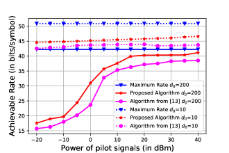
Refer to caption
Figure 4: Achievable rate vs. the transmit power of the pilot signals (in dBm).

V-B Convergence of The Proposed Algorithm

We now numerically evaluate the convergence of the upper bound of the proposed algorithm, given by (27). We also compare the actual probability, given by (26), that we obtain by simulations.

In Fig. 5, we show the convergence property of the error probability and its upper bound of the proposed algorithm for increasing values of ϵ={0.01,0.05,0.1}italic-ϵ0.010.050.1\epsilon=\{0.01,0.05,0.1\} when the power of the pilot signal is P=10𝑃10P=10 dBm and d0=200subscript𝑑0200d_{0}=200 m. We run the simulation for 1000 times. We see that for each value of ϵitalic-ϵ\epsilon, the proposed algorithm converges towards zero as we increase the number of pilots. Moreover, the upper bound of the error probability also converges to the error probability as the number of pilot signals increases.
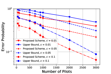
Refer to caption
Figure 5: Error Probability Bound v/s Number of Pilots for ϵ={0.01,0.05,0.1}italic-ϵ0.010.050.1\epsilon=\{0.01,0.05,0.1\} for P=10𝑃10P=10 dBm.

In Fig. 6, we compare the convergence property of the error probability of the proposed algorithm with respect to ϵ=0.05italic-ϵ0.05\epsilon=0.05 and d0=200subscript𝑑0200d_{0}=200 m for different levels of power of the pilot signals, P={5,10,20}𝑃51020P=\{5,10,20\} dBm. As we increase the power of the pilot signals, the estimation accuracy of α1subscript𝛼1\alpha_{1} and α2subscript𝛼2\alpha_{2} increases and hence the error probability decreases. This is so because, as we increase the power of pilot signals the received signals will be less noisy which increases the chances of estimating the α1subscript𝛼1\alpha_{1} and α2subscript𝛼2\alpha_{2} more accurately.

Refer to caption
Figure 6: Error Probability Bound v/s Number of Pilots for ϵ=0.05italic-ϵ0.05\epsilon=0.05 for P={5,10,20}𝑃51020P=\{5,10,20\} dBm.

VI Conclusion

We investigated the problem of estimation of the optimal phase-shift at the HMT-assisted wireless communication system in a noisy environment. We proposed a learning algorithm to estimate the optimal phase-shifting parameters and showed that the probability that the phase-shifting parameters generated by the proposed algorithm to deviate by more than ϵitalic-ϵ\epsilon from the optimal values decay exponentially fast as the number of pilots grows. Our proposed algorithm exploited structural properties of the channel gains in the far-field regions.

Appendix

VI-A Proof of Proposition 1

Proof.

Let us define the following events.

An,m=|XnXm|>ϵ,An=|XnX|>ϵ2,formulae-sequencesubscript𝐴𝑛𝑚subscript𝑋𝑛subscript𝑋𝑚italic-ϵsubscript𝐴𝑛subscript𝑋𝑛𝑋italic-ϵ2\displaystyle A_{n,m}=\left\lvert X_{n}-X_{m}\right\rvert>\epsilon,\quad A_{n}=\left\lvert X_{n}-X\right\rvert>\frac{\epsilon}{2},
 and Am=|XmX|>ϵ2 and subscript𝐴𝑚subscript𝑋𝑚𝑋italic-ϵ2\displaystyle\quad\text{ and }\quad A_{m}=\left\lvert X_{m}-X\right\rvert>\frac{\epsilon}{2}

By the triangle inequality, we have

|XnXm||XnX|+|XmX|.subscript𝑋𝑛subscript𝑋𝑚subscript𝑋𝑛𝑋subscript𝑋𝑚𝑋\displaystyle\left\lvert X_{n}-X_{m}\right\rvert\leq\left\lvert X_{n}-X\right\rvert+\left\lvert X_{m}-X\right\rvert. (64)

Using (64), the event An,msubscript𝐴𝑛𝑚A_{n,m} can be written as

|XnXm|ϵ|XnX|+|XmX|ϵsubscript𝑋𝑛subscript𝑋𝑚italic-ϵsubscript𝑋𝑛𝑋subscript𝑋𝑚𝑋italic-ϵ\displaystyle\left\lvert X_{n}-X_{m}\right\rvert\geq\epsilon\implies\left\lvert X_{n}-X\right\rvert+\left\lvert X_{m}-X\right\rvert\geq\epsilon

Therefore, we have

An,msubscript𝐴𝑛𝑚\displaystyle A_{n,m} {|XnX|+|XXm|>ϵ}absentsubscript𝑋𝑛𝑋𝑋subscript𝑋𝑚italic-ϵ\displaystyle\subset\{|X_{n}-X|+|X-X_{m}|>\epsilon\}
{|XnX|>ϵ2|XXm|>ϵ2}absentsubscript𝑋𝑛𝑋italic-ϵ2𝑋subscript𝑋𝑚italic-ϵ2\displaystyle\subset\left\{|X_{n}-X|>\frac{\epsilon}{2}\bigcup|X-X_{m}|>\frac{\epsilon}{2}\right\} (65)

Note that for any two events A𝐴A and B𝐵B where AB𝐴𝐵A\subset B, then {A}{B}𝐴𝐵\mathbb{P}\left\{A\right\}\leq\mathbb{P}\left\{B\right\}. We use this fact in (65), and we get

{|XnXm|>ϵ}{|XnX|>ϵ2}+{|XmX|>ϵ2}subscript𝑋𝑛subscript𝑋𝑚italic-ϵsubscript𝑋𝑛𝑋italic-ϵ2subscript𝑋𝑚𝑋italic-ϵ2\displaystyle\mathbb{P}\left\{|X_{n}-X_{m}|>\epsilon\right\}\leq\mathbb{P}\left\{|X_{n}-X|>\frac{\epsilon}{2}\right\}+\mathbb{P}\left\{|X_{m}-X|>\frac{\epsilon}{2}\right\}\qed

VI-B Proof of Lemma 2

Proof.

We consider r(β1,β2)𝑟subscript𝛽1subscript𝛽2r(\beta_{1},\beta_{2}) as given in (3) which comprises of two complex-valued factors P×H(β1,β2)𝑃𝐻subscript𝛽1subscript𝛽2\sqrt{P}\times H(\beta_{1},\beta_{2}) (see (1)) and ζ𝜁\zeta.

Write ζ=n1+jn2𝜁subscript𝑛1𝑗subscript𝑛2\zeta=n_{1}+jn_{2}, where n1subscript𝑛1n_{1} and n2subscript𝑛2n_{2} follows N(0,σ22)𝑁0superscript𝜎22N\left(0,\frac{\sigma^{2}}{2}\right) and are independent, and write P×H(β1,β2)=a+jb𝑃𝐻subscript𝛽1subscript𝛽2𝑎𝑗𝑏\sqrt{P}\times H(\beta_{1},\beta_{2})=a+jb, where a𝑎a and b𝑏b are real values. Therefore,

r(β1,β2)=|y(β1,β2)|2=(a+n1)2+(b+n2)2.𝑟subscript𝛽1subscript𝛽2superscript𝑦subscript𝛽1subscript𝛽22superscript𝑎subscript𝑛12superscript𝑏subscript𝑛22\displaystyle r(\beta_{1},\beta_{2})=\left\lvert y(\beta_{1},\beta_{2})\right\rvert^{2}=(a+n_{1})^{2}+(b+n_{2})^{2}. (66)

Note that a+n1σ/2N(aσ/2,1)similar-to𝑎subscript𝑛1𝜎2𝑁𝑎𝜎21\frac{a+n_{1}}{\sigma/\sqrt{2}}\sim N\left(\frac{a}{\sigma/\sqrt{2}},1\right) and b+n2σ/2N(bσ/2,1)similar-to𝑏subscript𝑛2𝜎2𝑁𝑏𝜎21\frac{b+n_{2}}{\sigma/\sqrt{2}}\sim N\left(\frac{b}{\sigma/\sqrt{2}},1\right) and they are independent. Therefore,

2σ2{(a+n1)2+(b+n2)2}χ22(2σ2(a2+b2)).similar-to2superscript𝜎2superscript𝑎subscript𝑛12superscript𝑏subscript𝑛22subscriptsuperscript𝜒222superscript𝜎2superscript𝑎2superscript𝑏2\displaystyle\frac{2}{\sigma^{2}}\bigg{\{}(a+n_{1})^{2}+(b+n_{2})^{2}\bigg{\}}\sim\chi^{2}_{2}\left(\frac{2}{\sigma^{2}}\left(a^{2}+b^{2}\right)\right). (67)

Applying (67) in (66), we get X=2σ2r(β1,β2)χ22(λ1),𝑋2superscript𝜎2𝑟subscript𝛽1subscript𝛽2similar-tosubscriptsuperscript𝜒22subscript𝜆1X=\frac{2}{\sigma^{2}}r(\beta_{1},\beta_{2})\sim\chi^{2}_{2}\left(\lambda_{1}\right), where λ1=2σ2|P×H(β1,β2)|2.subscript𝜆12superscript𝜎2superscript𝑃𝐻subscript𝛽1subscript𝛽22\lambda_{1}=\frac{2}{\sigma^{2}}\left\lvert\sqrt{P}\times H(\beta_{1},\beta_{2})\right\rvert^{2}. The second part of the lemma follows from the additive property of non-central Chi-squared distribution of the sum of n𝑛n i.i.d. RVs of χ22(λ1).subscriptsuperscript𝜒22subscript𝜆1\chi^{2}_{2}\left(\lambda_{1}\right).

VI-C Proof of Theorem 3

As Xk,ksubscript𝑋𝑘for-all𝑘X_{k},\forall k are independent, applying the definition IV.1, the moment generating function of k=1n(Xkμk)superscriptsubscript𝑘1𝑛subscript𝑋𝑘subscript𝜇𝑘\sum\limits_{k=1}^{n}(X_{k}-\mu_{k}) is given by

𝔼[etk=1n(Xkμk)]𝔼delimited-[]superscript𝑒𝑡superscriptsubscript𝑘1𝑛subscript𝑋𝑘subscript𝜇𝑘\displaystyle\mathbb{E}\left[e^{t\sum\limits_{k=1}^{n}(X_{k}-\mu_{k})}\right] eλ22k=1nνk2,|t|<(1maxk=1,2,,nbk).formulae-sequenceabsentsuperscript𝑒superscript𝜆22superscriptsubscript𝑘1𝑛superscriptsubscript𝜈𝑘2for-all𝑡1subscript𝑘12𝑛subscript𝑏𝑘\displaystyle\leq e^{\frac{\lambda^{2}}{2}\sum\limits_{k=1}^{n}\nu_{k}^{2}},\quad\forall|t|<\left(\frac{1}{\max\limits_{k=1,2,\dots,n}b_{k}}\right).

Since the moment generating functions uniquely determines the distribution, comparing with the definition IV.1, it follows that k=1n(Xkμk)superscriptsubscript𝑘1𝑛subscript𝑋𝑘subscript𝜇𝑘\sum\limits_{k=1}^{n}(X_{k}-\mu_{k}) is a sub-exponential (ν,b)subscript𝜈subscript𝑏(\nu_{*},b_{*}) random variable, where

b=maxk=1,2,nbkandν=k=1nνk2.formulae-sequencesubscript𝑏subscript𝑘12𝑛subscript𝑏𝑘andsubscript𝜈superscriptsubscript𝑘1𝑛superscriptsubscript𝜈𝑘2b_{*}=\max\limits_{k=1,2\dots,n}b_{k}\quad\text{and}\quad\nu_{*}=\sqrt{\sum\limits_{k=1}^{n}\nu_{k}^{2}}.

To prove the second part of the Theorem we use the following tail bound on a sub-exponential distribution proved in [18].

Proposition 1 ([18] Proposition 2.9).

Let X𝑋X is sub-exponential random variable with parameters (ν,b)𝜈𝑏(\nu,b) and 𝔼[X]=μ𝔼delimited-[]𝑋𝜇\mathbb{E}\left[X\right]=\mu. Then

{|Xμ|t}{2et22ν2,if 0tν2b2et2b,if tν2b.𝑋𝜇𝑡casesotherwise2superscript𝑒superscript𝑡22superscript𝜈2if 0𝑡superscript𝜈2𝑏otherwise2superscript𝑒𝑡2𝑏if 𝑡superscript𝜈2𝑏\displaystyle\mathbb{P}\left\{\left\lvert X-\mu\right\rvert\geq t\right\}\leq\begin{cases}&2e^{-\frac{t^{2}}{2\nu^{2}}},\qquad\text{if }0\leq t\leq\frac{\nu^{2}}{b}\\ &2e^{-\frac{t}{2b}},\qquad\text{if }t\geq\frac{\nu^{2}}{b}.\end{cases}

The claim immediately follows by applying the above result on Zn:=k=1n(Xkμk),assignsubscript𝑍𝑛superscriptsubscript𝑘1𝑛subscript𝑋𝑘subscript𝜇𝑘Z_{n}:=\sum\limits_{k=1}^{n}(X_{k}-\mu_{k}), which is sub-exponential (ν,b),subscript𝜈subscript𝑏(\nu_{*},b_{*}), where b=maxk=1,2,nbksubscript𝑏subscript𝑘12𝑛subscript𝑏𝑘b_{*}=\max\limits_{k=1,2\dots,n}b_{k} and ν=k=1nνk2subscript𝜈superscriptsubscript𝑘1𝑛superscriptsubscript𝜈𝑘2\nu_{*}=\sqrt{\sum\limits_{k=1}^{n}\nu_{k}^{2}}. ∎

VI-D Proof of Corollary 1

From Theorem 3, k=1n(Xkμk)superscriptsubscript𝑘1𝑛subscript𝑋𝑘subscript𝜇𝑘\sum_{k=1}^{n}(X_{k}-\mu_{k}) is sub-exponential (ν,b),subscript𝜈subscript𝑏(\nu_{*},b_{*}), where b=4subscript𝑏4b_{*}=4 and ν=2n(2+2a)subscript𝜈2𝑛22𝑎\nu_{*}=2\sqrt{n}(2+2a). Using the parameters (ν,b)=(2n(2+2a),4)subscript𝜈subscript𝑏2𝑛22𝑎4(\nu_{*},b_{*})=(2\sqrt{n}(2+2a),4) in Proposition 1, we get the required upper bound as

{|1nk=1n(Xkμk)|t}{2ent28(2+2a)2,0t(2+2a)22ent8,t(2+2a)21𝑛superscriptsubscript𝑘1𝑛subscript𝑋𝑘subscript𝜇𝑘𝑡cases2superscript𝑒𝑛superscript𝑡28superscript22𝑎20𝑡superscript22𝑎22superscript𝑒𝑛𝑡8𝑡superscript22𝑎2\displaystyle\mathbb{P}\left\{\left\lvert\frac{1}{n}\sum\limits_{k=1}^{n}(X_{k}-\mu_{k})\right\rvert\geq t\right\}\leq\begin{cases}2e^{-\frac{nt^{2}}{8(2+2a)^{2}}},&0\leq t\leq(2+2a)^{2}\\ 2e^{-\frac{nt}{8}},&t\geq(2+2a)^{2}\\ \end{cases}
{|1nk=1n(Xkμk)|t}2ent28(2+2a)2,t>0.formulae-sequence1𝑛superscriptsubscript𝑘1𝑛subscript𝑋𝑘subscript𝜇𝑘𝑡2superscript𝑒𝑛superscript𝑡28superscript22𝑎2𝑡0\displaystyle\mathbb{P}\left\{\left\lvert\frac{1}{n}\sum\limits_{k=1}^{n}(X_{k}-\mu_{k})\right\rvert\geq t\right\}\leq 2e^{-\frac{nt^{2}}{8(2+2a)^{2}}},\qquad t>0.

VI-E Proof of Lemma 3

If Xχp2(a)similar-to𝑋superscriptsubscript𝜒𝑝2𝑎X\sim\chi_{p}^{2}(a), then according to [20], the moment-generating function (MGF) of X𝑋X is given by

𝔼[exp{t(X(p+a)}]\displaystyle\mathbb{E}\left[\exp\{t(X-(p+a)\}\right] =et(p+a)𝔼[etX]absentsuperscript𝑒𝑡𝑝𝑎𝔼delimited-[]superscript𝑒𝑡𝑋\displaystyle=e^{-t(p+a)}\mathbb{E}\left[e^{tX}\right]
=et(p+a)eat12t(12t)p/2absentsuperscript𝑒𝑡𝑝𝑎superscript𝑒𝑎𝑡12𝑡superscript12𝑡𝑝2\displaystyle=\frac{e^{-t(p+a)}e^{\frac{at}{1-2t}}}{(1-2t)^{p/2}}
=e2at212tept(12t)p/2, for t<12.formulae-sequenceabsentsuperscript𝑒2𝑎superscript𝑡212𝑡superscript𝑒𝑝𝑡superscript12𝑡𝑝2 for 𝑡12\displaystyle=e^{\frac{2at^{2}}{1-2t}}\frac{e^{-pt}}{(1-2t)^{p/2}},\qquad\text{ for }t<\frac{1}{2}. (68)

By following some calculus, refer [21], [18, Example 2.8], we obtain

ept(12t)p/2e2pt2, for |t|14.formulae-sequencesuperscript𝑒𝑝𝑡superscript12𝑡𝑝2superscript𝑒2𝑝superscript𝑡2 for 𝑡14\displaystyle\frac{e^{-pt}}{(1-2t)^{p/2}}\leq e^{2pt^{2}},\qquad\text{ for }\left\lvert t\right\rvert\leq\frac{1}{4}. (69)

For |t|14𝑡14\left\lvert t\right\rvert\leq\frac{1}{4}, we have

e2at212te4at2.superscript𝑒2𝑎superscript𝑡212𝑡superscript𝑒4𝑎superscript𝑡2\displaystyle e^{\frac{2at^{2}}{1-2t}}\leq e^{4at^{2}}. (70)

Applying (69) and (70) to (68), we obtain

𝔼[exp{t(X(p+a)}]e2(p+2a)t2,|t|14.\displaystyle\mathbb{E}\left[\exp\{t(X-(p+a)\}\right]\leq e^{2(p+2a)t^{2}},\qquad\forall\left\lvert t\right\rvert\leq\frac{1}{4}. (71)

Therefore, by (71), X𝑋X is Sub-exponential distribution with parameters (2(p+2a),4).2𝑝2𝑎4\big{(}2(p+2a),4\big{)}.

References

  • [1] Z. Wan, Z. Gao, F. Gao, M. Di Renzo, and M.-S. Alouini, “Terahertz massive mimo with holographic reconfigurable intelligent surfaces,” IEEE Transactions on Communications, 2021.
  • [2] V. Jamali, A. M. Tulino, G. Fischer, R. R. Müller, and R. Schober, “Intelligent surface-aided transmitter architectures for millimeter-wave ultra massive mimo systems,” IEEE Open Journal of the Communications Society, vol. 2, pp. 144–167, 2020.
  • [3] E. G. Larsson, O. Edfors, F. Tufvesson, and T. L. Marzetta, “Massive mimo for next generation wireless systems,” IEEE communications magazine, vol. 52, no. 2, pp. 186–195, 2014.
  • [4] Q. Wu and R. Zhang, “Intelligent reflecting surface enhanced wireless network via joint active and passive beamforming,” IEEE Transactions on Wireless Communications, vol. 18, no. 11, pp. 5394–5409, 2019.
  • [5] C. Huang, S. Hu, G. C. Alexandropoulos, A. Zappone, C. Yuen, R. Zhang, M. Di Renzo, and M. Debbah, “Holographic mimo surfaces for 6g wireless networks: Opportunities, challenges, and trends,” IEEE Wireless Communications, vol. 27, no. 5, pp. 118–125, 2020.
  • [6] S. Hu, F. Rusek, and O. Edfors, “Beyond massive mimo: The potential of data transmission with large intelligent surfaces,” IEEE Transactions on Signal Processing, vol. 66, no. 10, pp. 2746–2758, 2018.
  • [7] I. Yoo and D. R. Smith, “Holographic metasurface antennas for uplink massive mimo systems,” arXiv preprint arXiv:2108.12513, 2021.
  • [8] H. Zhang, N. Shlezinger, F. Guidi, D. Dardari, M. F. Imani, and Y. C. Eldar, “Beam focusing for near-field multi-user mimo communications,” IEEE Transactions on Wireless Communications, 2022.
  • [9] F. Dai and J. Wu, “Efficient broadcasting in ad hoc wireless networks using directional antennas,” IEEE Transactions on Parallel and Distributed Systems, vol. 17, no. 4, pp. 335–347, 2006.
  • [10] Z. Xiao, T. He, P. Xia, and X.-G. Xia, “Hierarchical codebook design for beamforming training in millimeter-wave communication,” IEEE Transactions on Wireless Communications, vol. 15, no. 5, pp. 3380–3392, 2016.
  • [11] K. Chen and C. Qi, “Beam training based on dynamic hierarchical codebook for millimeter wave massive mimo,” IEEE Communications Letters, vol. 23, no. 1, pp. 132–135, 2018.
  • [12] Ö. T. Demir, E. Björnson, and L. Sanguinetti, “Channel modeling and channel estimation for holographic massive mimo with planar arrays,” IEEE Wireless Communications Letters, vol. 11, no. 5, pp. 997–1001, 2022.
  • [13] M. Ghermezcheshmeh, V. Jamali, H. Gacanin, and N. Zlatanov, “Channel estimation for large intelligent surface-based transceiver using a parametric channel model,” arXiv preprint arXiv:2112.02874, 2021.
  • [14] M. R. Akdeniz, Y. Liu, M. K. Samimi, S. Sun, S. Rangan, T. S. Rappaport, and E. Erkip, “Millimeter wave channel modeling and cellular capacity evaluation,” IEEE journal on selected areas in communications, vol. 32, no. 6, pp. 1164–1179, 2014.
  • [15] S. W. Ellingson, “Path loss in reconfigurable intelligent surface-enabled channels,” in 2021 IEEE 32nd Annual International Symposium on Personal, Indoor and Mobile Radio Communications (PIMRC).   IEEE, 2021, pp. 829–835.
  • [16] K. T. Selvan and R. Janaswamy, “Fraunhofer and fresnel distances: Unified derivation for aperture antennas.” IEEE Antennas and Propagation Magazine, vol. 59, no. 4, pp. 12–15, 2017.
  • [17] M. Najafi, V. Jamali, R. Schober, and H. V. Poor, “Physics-based modeling and scalable optimization of large intelligent reflecting surfaces,” IEEE Transactions on Communications, vol. 69, no. 4, pp. 2673–2691, 2020.
  • [18] M. J. Wainwright, High-dimensional statistics: A non-asymptotic viewpoint.   Cambridge University Press, 2019, vol. 48.
  • [19] W. Wang and W. Zhang, “Joint beam training and positioning for intelligent reflecting surfaces assisted millimeter wave communications,” IEEE Transactions on Wireless Communications, vol. 20, no. 10, pp. 6282–6297, 2021.
  • [20] A. E. El-Sayed, A. I. Sahar, and Y. A. Yassmen, “Moment generating function of the unbalanced non-central chi-square distribution,” International Journal of Engineering, vol. 4, no. 3, p. 8269, 2013.
  • [21] M. Ghosh, “Exponential tail bounds for chisquared random variables,” Journal of Statistical Theory and Practice, vol. 15, no. 2, pp. 1–6, 2021.