Exciton spectrum in atomically thin monolayers:
The role of hBN encapsulation

Abstract

The high-quality structures containing semiconducting transition metal dichalcogenides (S-TMDs) monolayer (MLs) required for optical and electrical studies are achieved by their encapsulation in hexagonal BN (hBN) flakes. To examine the effect of hBN thickness in these systems, we consider a model with an S-TMD ML placed between a semi-infinite in the out-of-plane direction substrate and complex top cover layers: a layer of finite thickness, adjacent to the ML, and a semi-infinite in the out-of-plane direction top part. We obtain the expression for the Coulomb potential for such a structure. Using this result, we demonstrate that the energies of excitonic $s$ states in the structure with WSe₂ ML change significantly for the top hBN with thickness less than 30 layers for different substrate cases, such as hBN and SiO₂. For the larger thickness of the top hBN flake, the binding energies of the excitons are saturated to their values of the bulk hBN limit.

I Introduction

The properties of excitons, electron-hole ($e$-$h$) pairs bounded by Coulomb force, in two-dimensional (2D) monolayers (MLs) of semiconducting transition metal dichalcogenides (S-TMDs) are remarkably modified due to a significant change in the Coulomb interaction between charge carriers in such 2D crystals [1, 2, 3]. The excitons are characterized by the energy spectrum, composed in analogy to the hydrogen series as of the ground (1$s$) and excited (2$s$, $2p$, 3$s$ $\dots$) states. Although excitonic states of the $s$-type are observable in the linear optical spectra of S-TMD MLs, $i.e.$, photoluminescence [4, 5, 6, 7, 8], transmission [9, 10, 11], and reflectance contrast [12, 6, 13], the excitonic states of the $p$- and $d$-types can be seen in non-linear experiments performed on S-TMD MLs, $i.e.$, second harmonic generation or two-photon absorption [14, 15, 16, 17]. It turns out that the energy spectrum of $s$-type states in these atomically-thin semiconductors does not reproduce the conventional Rydberg series of a 2D hydrogen atom [18, 19]. The main reason for that is the dielectric inhomogeneity of the S-TMD structures, $i.e.$, MLs surrounded by dielectric materials. While the Coulomb interaction scales as $\propto 1/\varepsilon r$ with the dielectric response of the surrounding medium $\varepsilon$ at large $e$-$h$ distances $r$, it appears to be significantly weakened at short $e$-$h$ distances due to exceptionally strong dielectric screening within the ML plane. Consequently, the energy spectrum of excitons in S-TMD MLs and hence their binding energy, defined as the energy difference between the electronic band gap and the ground 1$s$ state, can be strongly modified by the used surrounding media of different dielectric responses.

The influence of the surrounding dielectric on the excitonic ladder has been studied both experimentally and theoretically [12, 20, 21, 9, 6, 10, 22, 23, 24, 25, 26, 11]. Note that the theoretical approaches rely mostly on the ab initio [27, 28, 29, 30], as well as the combination of the ab initio and analytical methods [31, 32]. In the latter case, the results of ab initio simulations have been used as input parameters for the analytical models, which are called quantum electrostatic heterostructure (QEH) models. Such the incoming parameters are dielectric functions of the multilayer van der Waals heterostructure [31, 28], momentum dependent matrix elements of the screened Coulomb interaction and the band structure of the valence and conduction bands [30], or even the modified Coulomb potential $V_{3\chi}(\rho)$ in Ref. [32]. However, in all these cases the calculation of the excitons’ energies requires large computational powers. Therefore, the QEH model, which takes into account all the basic characteristics of the heterostructure, but requires less computational resources to calculate the excitonic spectrum, is still needed.

Note that the current approach to obtain the highest-quality S-TMD MLs is based on their encapsulation in flakes of atomically flat hexagonal BN (hBN). It results, in particular, in a substantial narrowing of excitonic resonances approaching the homogeneous linewidth limit [33, 34, 35], that allows to identify precisely their spectrum. Consequently, it is of the utmost importance to perform theoretical calculations of the thickness influence of the surrounding media on the excitons spectra in S-TMD MLs within the aforementioned QEH model.

In this work, we investigate theoretically the energy spectrum of free excitons in S-TMD MLs encapsulated in between a semi-infinite in the out-of-plane direction bottom substrate and complex top cover layers consisting of two parts: a layer of finite thickness $L$, adjacent to the ML, and semi-infinite in the out-of-plane direction top part with the aid of generalization of the Rytova-Keldysh potential. We demonstrate that the energies of the excitonic $s$ states in such a system with the WSe₂ ML are strongly modified when the thickness of the top hBN layers decreases below about 30 layers. In addition, it results in a significant reduction in excitonic binding energy ($E_{\mathrm{b}}$) of almost 40% in the transition from the sample without the top hBN layer ($E_{\mathrm{b}}$=256 meV) to the one with an infinite thickness of the top hBN layer ($E_{\mathrm{b}}$=165 meV). The similar behavior of the binding energies as a function of the thickness of the top hBN layer has been observed for the other type of substrates.

The paper is organized as follows. In Sec. II, we present the theoretical framework for the calculation of the effective Coulomb potential in a non-homogeneous planar system, presented in Fig. 1. We analyze the analytical expression for the potential in momentum as well as in coordinate space, as a function of the parameters of the system. In Sec. III we consider the particular case of the hBN substrate and hBN top flake of finite thickness $L$, and calculate the corresponding effective Coulomb potential for this case. Using the obtained potential, we calculate in Sec. IV the energy ladder of the excitons for the case of the WSe₂ monolayer as a function of the number of layers of the top hBN flake. In Sec. V, we summarize all findings. Moreover, the Supplementary Material (SM) presents additional calculations that take into account the discrete structure of the top hBN layer. Using this result, we obtain the spectrum of the excitons in WSe₂ monolayer with mono- and bilayer top hBN layer and compare the result found within the model proposed in the main text. We also study the role of the non-zero distance $\delta$ between the monolayer and the sub- and superstrate on the excitonic spectrum in such a system.

II Coulomb potential in the non-homogeneous system: general case

Let us consider the S-TMD ML encapsulated in between a semi-infinite bottom substrate (1-st layer) and complex top cover layers consisting of two parts: 2-nd layer of finite thickness $L$, adjacent to the ML, and semi-infinite in the out-of-plane direction 3-rd part. A schematic illustration of the studied system is presented in Fig. 1. The ML is arranged in the $xy$ plane and is centered in the out-of-plane direction ($z=0$). The bottom substrate, 1-st layer, belongs to the domain $z\in]-\infty,-\delta]$, and is characterized by the in-plane $\varepsilon_{1,\parallel}$ and out-of-plane $\varepsilon_{1,\perp}$ dielectric constants. The top (2-nd) layer, next to the ML, unfolds in the range $z\in[\delta,L]$ with the in-plane $\varepsilon_{2,\parallel}$ and out-of-plane $\varepsilon_{2,\perp}$ dielectric constants. Finally, the 3-rd top layer spreads over the distance $z\in[L,\infty[$ and is described by the in-plane $\varepsilon_{3,\parallel}$ and out-of-plane $\varepsilon_{3,\perp}$ dielectric constants.

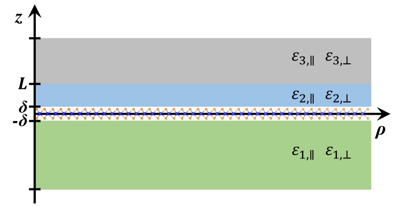
Figure 1: The schematic illustration of the S-TMD monolayer encapsulated in between a semi-infinite bottom substrate (1-st layer) and a complex top cover layers consisting of two parts: 2-nd layer of the finite thickness, adjacent to the ML and semi-infinite in the out-of-plane direction 3-rd part.

To find the potential energy between two charges in S-TMD MLs, we solve the following electrostatic problem. We investigate the point-like charge $Q$ at the point $\mathbf{r}=(\bm{\rho},z)=(0,0,0)$ and calculate the electric potential in such a system following Refs. [36, 37]. Namely, we analyze four regions: bottom ($z\in]-\infty,-\delta]$), ML ($z\in[-\delta,\delta]$), top finite ($z\in[\delta,L]$) and overtop ($z\in[L,\infty[$) media, with potentials $\Phi_{1}(\bm{\rho},z)$, $\Phi(\bm{\rho},z)$, $\Phi_{2}(\bm{\rho},z)$, and $\Phi_{3}(\bm{\rho},z)$, respectively. These potentials are defined by the Maxwell equations. It is convenient to present the potentials as a Fourier transform

$$\Phi_{j}(\bm{\rho},z)= \frac{1}{(2\pi)^{2}}\int d^{2}\mathbf{k}e^{i\mathbf{k}\bm{\rho}}\Phi_{j}(\mathbf{k},z),$$ (1)

$$\Phi(\bm{\rho},z)= \frac{1}{(2\pi)^{2}}\int d^{2}\mathbf{k}e^{i\mathbf{k}\bm{\rho}}\Phi(\mathbf{k},z).$$ (2)

The $\Phi_{j}(\bm{\rho},z)$ potentials for the $j$-th region, where $j=1,2,3$, satisfy Maxwell’s equation $\mathrm{div}\,\mathbf{D}_{j}(\bm{\rho},z)=0$, which can be written as

$$-\varepsilon_{j,\parallel}\mathbf{k}^{2}\Phi_{j}(\mathbf{k},z)+\varepsilon_{j,\perp}\frac{d^{2}\Phi_{j}(\mathbf{k},z)}{dz^{2}}=0.$$ (3)

The solutions of these equations are

$$\Phi_{1}(\mathbf{k},z) =B_{1}e^{\kappa_{1}z} ~{}z\in]-\infty,-\delta],$$ for (4)

$$\Phi_{2}(\mathbf{k},z) =A_{2}e^{-\kappa_{2}z}+B_{2}e^{\kappa_{2}z} z\in[\delta,L],$$ for (5)

$$\Phi_{3}(\mathbf{k},z) =A_{3}e^{-\kappa_{3}z} z\in[L,\infty[,$$ for (6)

where $\kappa_{j}=|\mathbf{k}|\sqrt{\varepsilon_{j,\parallel}/\varepsilon_{j,\perp}}=k\sqrt{\varepsilon_{j,\parallel}/\varepsilon_{j,\perp}}$.

Maxwell’s equation in the ML domain, $i.e.$, $z\in[-\delta,\delta]$, reads $\text{div}\,\mathbf{D}(\bm{\rho},z)=4\pi Q\delta(\bm{\rho})\delta(z)$. It gives the equation for the potential $\Phi(\mathbf{r},z)$

$$\Big{[}\Delta_{\parallel}+\frac{d^{2}}{dz^{2}}\Big{]}\Phi(\bm{\rho},z)=-4\pi[Q\delta(\bm{\rho})\delta(z)-\varrho_{\text{ind}}(\bm{\rho},z)],$$ (7)

where $\Delta_{\parallel}$ is 2D Laplace operator. The first term in the right-hand-side of Eq. (7) is the charge density of the charge $Q$, localized in the ML plane. The second term represents the polarization charge density $\varrho_{\text{ind}}(\bm{\rho},z)$, induced in the ML by point charge $Q$, which is given by

$$\varrho_{\text{ind}}(\bm{\rho},z)=\mathrm{div}\,\mathbf{P}(\bm{\rho},z).$$ (8)

Following Ref. [36], we present the polarization in the form

$$\mathbf{P}(\bm{\rho},z)=\delta(z)\mathbf{P}_{\parallel}(\bm{\rho},z=0).$$ (9)

Using the proportionality between the induced polarization $\mathbf{P}_{\parallel}(\bm{\rho},0)$ and the in-plane component of the electric field $\mathbf{E}_{\parallel}(\bm{\rho},0)$, $\mathbf{P}_{\parallel}(\bm{\rho},0)=\chi_{\text{TMD}}\mathbf{E}_{\parallel}(\bm{\rho},0)$, we obtain the expression for the induced charge

$$\varrho_{\text{ind}}(\bm{\rho},z)=-\chi_{\text{TMD}}\delta(z)\Delta_{\parallel}\Phi(\bm{\rho},0).$$ (10)

Here $\chi_{\text{TMD}}$ is the 2D polarizability of the S-TMD monolayer [36, 38]. Introducing the screening length parameter $r_{0}=2\pi\chi_{\text{TMD}}$, and taking the Fourier transformation of Eq. (7) with the induced charge from Eq. (10), one gets

$$\Big{[}\mathbf{k}^{2}-\frac{d^{2}}{dz^{2}}\Big{]}\Phi(\mathbf{k},z)=4\pi Q\delta(z)-2r_{0}k^{2}\delta(z)\Phi(\mathbf{k},0).$$ (11)

This is a linear non-homogeneous differential equation of the second order, which solution can be presented as a sum of the general solution of the homogeneous equation and a particular solution of the non-homogeneous equation (see Ref. [39] and Supplementary Material)

$$\Phi(\mathbf{k},z)=\Psi e^{-k|z|}+Ae^{-kz}+Be^{kz}.$$ (12)

The $k$-dependent parameters of the potential $\Psi$, $A$, and $B$ are not independent. The relations between them are defined from Eq. (7). Integrating it over $z$ in the domain $z\in[-\epsilon,\epsilon]$ and then taking the limit $\epsilon\rightarrow 0$, one obtains

$$[1+r_{0}k]\Psi+r_{0}k[A+B]=\frac{2\pi Q}{k}.$$ (13)

Using the continuity of the potential and $z$ component of the displacement field $\mathbf{D}(\bm{\rho},z)$ on the boundary of two adjusted domains, one obtains the set of equations for the parameters $\Psi$, $A$, $B$, $B_{1}$, $A_{2}$, $B_{2}$, $A_{3}$. The boundary conditions for the 1-st and ML domains give relations

$$B_{1}e^{-\kappa_{1}\delta} =\Psi e^{-k\delta}+Ae^{k\delta}+Be^{-k\delta},$$ (14)

$$\varepsilon_{1}B_{1}e^{-\kappa_{1}\delta} =\Psi e^{-k\delta}-Ae^{k\delta}+Be^{-k\delta}.$$ (15)

The boundary conditions between the ML and 2-nd domains are described by equations

$$A_{2}e^{-\kappa_{2}\delta}+B_{2}e^{\kappa_{2}\delta} =\Psi e^{-k\delta}+Ae^{-k\delta}+Be^{k\delta},$$ (16)

$$\varepsilon_{2}A_{2}e^{-\kappa_{2}\delta}-\varepsilon_{2}B_{2}e^{\kappa_{2}\delta} =\Psi e^{-k\delta}+Ae^{-k\delta}-Be^{k\delta}.$$ (17)

Finally, the boundary conditions between the 2-nd and 3-rd domains give

$$A_{2}e^{-\kappa_{2}L}+B_{2}e^{\kappa_{2}L} =A_{3}e^{-\kappa_{3}L},$$ (18)

$$\varepsilon_{2}A_{2}e^{-\kappa_{2}L}-\varepsilon_{2}B_{2}e^{\kappa_{2}L} =\varepsilon_{3}A_{3}e^{-\kappa_{3}L}.$$ (19)

Here, we introduce $\varepsilon_{j}=\sqrt{\varepsilon_{j,\perp}\varepsilon_{j,\parallel}}$ for $j=1,2,3$. Solving these equations together with Eq. (13), we obtain the values of the $\Psi$, $A$, and $B$ parameters. Then substituting them into the expression $\Phi(\mathbf{k},z=0)=\Psi+A+B=2\pi Q/k\varepsilon(k)$ we obtain the effective in-plane Coulomb potential $\Phi(\mathbf{k},z=0)$. Here $\varepsilon(k)$ is the dielectric function of the system

$$\varepsilon(k)=kr_{0}+\frac{1-\Big{(}\frac{\varepsilon_{1}-1}{\varepsilon_{1}+1}\Big{)}\Big{(}\frac{\varepsilon_{2}-1}{\varepsilon_{2}+1}\Big{)}e^{-4k\delta}-\Big{(}\frac{\varepsilon_{2}-\varepsilon_{3}}{\varepsilon_{2}+\varepsilon_{3}}\Big{)}\Big{[}\Big{(}\frac{\varepsilon_{2}-1}{\varepsilon_{2}+1}\Big{)}-\Big{(}\frac{\varepsilon_{1}-1}{\varepsilon_{1}+1}\Big{)}e^{-4k\delta}\Big{]}e^{-2\kappa_{2}(L-\delta)}}{\Big{[}1-\Big{(}\frac{\varepsilon_{1}-1}{\varepsilon_{1}+1}\Big{)}e^{-2k\delta}\Big{]}\Big{[}1-\Big{(}\frac{\varepsilon_{2}-1}{\varepsilon_{2}+1}\Big{)}e^{-2k\delta}+\Big{(}\frac{\varepsilon_{2}-\varepsilon_{3}}{\varepsilon_{2}+\varepsilon_{3}}\Big{)}\Big{[}e^{-2k\delta}-\Big{(}\frac{\varepsilon_{2}-1}{\varepsilon_{2}+1}\Big{)}\Big{]}e^{-2\kappa_{2}(L-\delta)}\Big{]}}.$$ (20)

The coordinate-dependent potential $\Phi(\bm{\rho})$ for the considered non-homogeneous system with the dielectric function $\varepsilon(k)$ then reads

$$\Phi(\bm{\rho})=Q\int_{0}^{\infty}dk\frac{J_{0}(k\rho)}{\varepsilon(k)},$$ (21)

where $J_{0}(x)$ is the zeroth Bessel function of the first kind. One can see that the information about the studied heterostructure is fully contained in the second part of the expression. Note that the expression for the in-plane potential contains only the combinations $\varepsilon_{j}=\sqrt{\varepsilon_{j,\parallel}\varepsilon_{j,\perp}}$ and $\kappa_{2}=k\sqrt{\varepsilon_{2,\parallel}/\varepsilon_{2,\perp}}$.

The expression (20) simplifies in two important limits. The limit $L\rightarrow\infty$ provides

$$\varepsilon(k)=kr_{0}-1+\sum_{j=1,2}\frac{1}{1-\Big{(}\frac{\varepsilon_{j}-1}{\varepsilon_{j}+1}\Big{)}e^{-2k\delta}}.$$ (22)

This formula interpolates between the case of suspended monolayer $\delta\rightarrow\infty$ ($\varepsilon(k)=kr_{0}+1$) and the case of monolayer, encapsulated between two media with dielectric constants $\varepsilon_{1},\varepsilon_{2}$, $\delta\rightarrow 0$ ($\varepsilon(k)=kr_{0}+[\varepsilon_{1}+\varepsilon_{2}]/2$). Both limit cases correspond to the so-called Rytova-Keldysh potential in coordinate space, first derived in Refs. [37, 40].

Another limit of Eq. (20), which corresponds to the situation with zero distance $\delta\rightarrow 0$ between the S-TMD monolayer and the dielectric media, provides

$$\varepsilon(k)=kr_{0}+\frac{\varepsilon_{1}-\varepsilon_{2}}{2}+\frac{\varepsilon_{2}}{1+\Big{(}\frac{\varepsilon_{2}-\varepsilon_{3}}{\varepsilon_{2}+\varepsilon_{3}}\Big{)}e^{-2\kappa_{2}L}}.$$ (23)

We consider this dielectric function as the simplest extension of the Rytova-Keldysh model for the case of finite thickness $L$ of the superstrate.

One can see that the key parameter that regulates the shape of $\varepsilon(k)$ is $\tau=\exp(-2\kappa_{2}L)$. Namely, the long-wavelength $\lambda(k)=2\pi/k\rightarrow\infty$ and short-wavelength $\lambda(k)=2\pi/k\rightarrow 0$ limits correspond to $\tau\rightarrow 1$ and $\tau\rightarrow 0$ cases, respectively. In the long-wavelength limit, the dielectric constant is $\varepsilon(k)\rightarrow(\varepsilon_{1}+\varepsilon_{3})/2$. This result reflects the fact that in this case most of the electric field lines occupy the bottom and second-top regions. In this case, neither the S-TMD monolayer nor the thin first top layer contributes significantly to the dielectric response of the system, due to their small volumes in comparison to the volumes of the other regions. The expression for the potential takes the form $\Phi(\mathbf{k},z=0)\rightarrow 2\pi Q/(k[\varepsilon_{1}+\varepsilon_{3}]/2)$. It provides the following large distance, $\rho\rightarrow\infty$, the behavior of the potential in the coordinate space $\Phi(\rho,z=0)\rightarrow Q/(\rho[\varepsilon_{1}+\varepsilon_{3}]/2)$, which is nothing more than the Coulomb potential of point charge $Q$ placed in between two substrates with dielectric constants $\varepsilon_{1}$ and $\varepsilon_{3}$, respectively.

In the opposite limit, $\lambda(k)\rightarrow 0$, the significant part of the electric lines of the charge occupies the monolayer, the first top layer, and bottom regions. In this case, the effective dielectric constant takes the form $\varepsilon(k)\rightarrow kr_{0}+(\varepsilon_{1}+\varepsilon_{2})/2$. As one can see, the second top substrate does not give a contribution to the potential. The corresponding limit defines the small distance, $\rho\rightarrow 0$, behavior of the potential $\Phi(\rho,z=0)\rightarrow(\pi Q/2)[\text{H}_{0}(\rho[\varepsilon_{1}+\varepsilon_{2}]/2r_{0})-Y_{0}(\rho[\varepsilon_{1}+\varepsilon_{2}]/2r_{0})]$.

Finally, note that both coordinate-dependent potentials also correspond to two limits $L\rightarrow 0$ and $L\rightarrow\infty$ of the thickness $L$ of the first top layer. Therefore, the potential with a finite value of $L$ interpolates between these two potentials, as is depicted in Fig. 3 for particular cases of dielectric constants of the surrounding media.

III The Coulomb potential in S-TMD sample: effect of finite thickness of hBN top layer

We examine the particular case of an S-TMD ML encapsulated in hBN layers, $i.e.$, $\varepsilon_{1,\parallel}=\varepsilon_{2,\parallel}=\varepsilon_{\text{hBN},\parallel}$, $\varepsilon_{1,\perp}=\varepsilon_{2,\perp}=\varepsilon_{\text{hBN},\perp}$, $\varepsilon_{3,\parallel}=\varepsilon_{3,\perp}=1$. Following the values available in the literature, we use $\varepsilon_{1}=\varepsilon_{2}=\varepsilon_{\text{hBN}}=4.5$, and $\kappa_{2}=k\sqrt{\varepsilon_{\text{hBN},\parallel}/\varepsilon_{\text{hBN},\perp}}\approx 1.098\,k$ [9]. Here we use the high-frequency (infrared) values for the dielectric constants of hBN. This is because the typical frequency scale at which the hBN flake responds to the excitons in the WSe₂ monolayer is given approximately by their binding energies of hundreds of meV, see more details in Refs. [20, 9, 41]. Note that $\varepsilon_{3,\parallel}=\varepsilon_{3,\perp}=1$ resemble typical experimental conditions, $i.e.$, the sample is placed in air, vacuum, or gaseous helium. Introducing the dimensionless momentum $x=kr_{0}/\varepsilon_{\text{hBN}}$ and length $l=\varepsilon_{\text{hBN}}L/r_{0}$ parameters, we obtain the following expression for the effective dielectric constant

$$\varepsilon(x,l)=\varepsilon_{\text{hBN}}x+\frac{\varepsilon_{\text{hBN}}}{1+\frac{\varepsilon_{\text{hBN}}-1}{\varepsilon_{\text{hBN}}+1}\exp\Big{(}-2\sqrt{\frac{\varepsilon_{\text{hBN},\parallel}}{\varepsilon_{\text{hBN},\perp}}}xl\Big{)}}.$$ (24)

This dielectric function, normalized for $\varepsilon_{\text{hBN}}$, for different values of the dimensionless thickness $l$ of the top hBN flake is presented in Fig. 2.

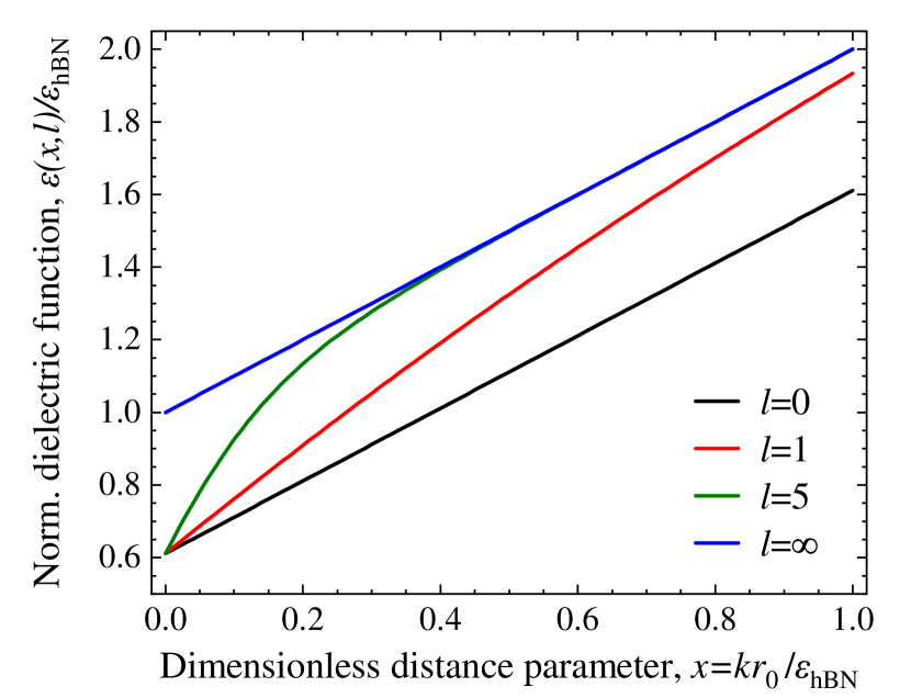
Figure 2: Normalized dielectric function $\varepsilon(x,l)/\varepsilon_{\text{hBN}}$ for four values of dimensionless length parameter, $l$: $l$=0, $l$=1, $l$=5, and $l$=$\infty$ (black, red, green, and blue curves, respectively) as a function of a dimensionless distance parameter, $x=kr_{0}/\varepsilon_{\text{hBN}}$.

The corresponding effective potential for the considered case $\Phi(\xi)=(Q/r_{0})\phi(\xi,l)$, as a function of the dimensionless distance $\xi=\rho\varepsilon_{\text{hBN}}/r_{0}$, reads

$$\phi(\xi,l)=\int_{0}^{\infty}dx\frac{J_{0}(x\xi)\Big{[}1+\frac{\varepsilon_{\text{hBN}}-1}{\varepsilon_{\text{hBN}}+1}\exp\Big{(}-2\sqrt{\frac{\varepsilon_{\text{hBN},\parallel}}{\varepsilon_{\text{hBN},\perp}}}xl\Big{)}\Big{]}}{1+x\Big{[}1+\frac{\varepsilon_{\text{hBN}}-1}{\varepsilon_{\text{hBN}}+1}\exp\Big{(}-2\sqrt{\frac{\varepsilon_{\text{hBN},\parallel}}{\varepsilon_{\text{hBN},\perp}}}xl\Big{)}\Big{]}}.$$ (25)

Note that in the limit $l\rightarrow\infty$, $i.e.$, an ML encapsulated in semi-infinite hBN layers, the potential expression is simplified and gives the well-known Rytova-Keldysh potential [40, 37]

$$\phi(\xi,\infty)=\int_{0}^{\infty}dx\frac{J_{0}(x\xi)}{1+x}=\frac{\pi}{2}\Big{[}\text{H}_{0}(\xi)-Y_{0}(\xi)\Big{]}.$$ (26)

The other limit $l\rightarrow 0$ corresponds to the case of an ML deposited on a semi-infinite hBN substrate, uncovered from the top. The related potential also has the Rytova-Keldysh form

$$\phi(\xi,0)=\frac{\pi}{2}\Big{[}\text{H}_{0}\Big{(}\frac{\varepsilon_{\text{hBN}}+1}{2\varepsilon_{\text{hBN}}}\xi\Big{)}-Y_{0}\Big{(}\frac{\varepsilon_{\text{hBN}}+1}{2\varepsilon_{\text{hBN}}}\xi\Big{)}\Big{]}.$$ (27)

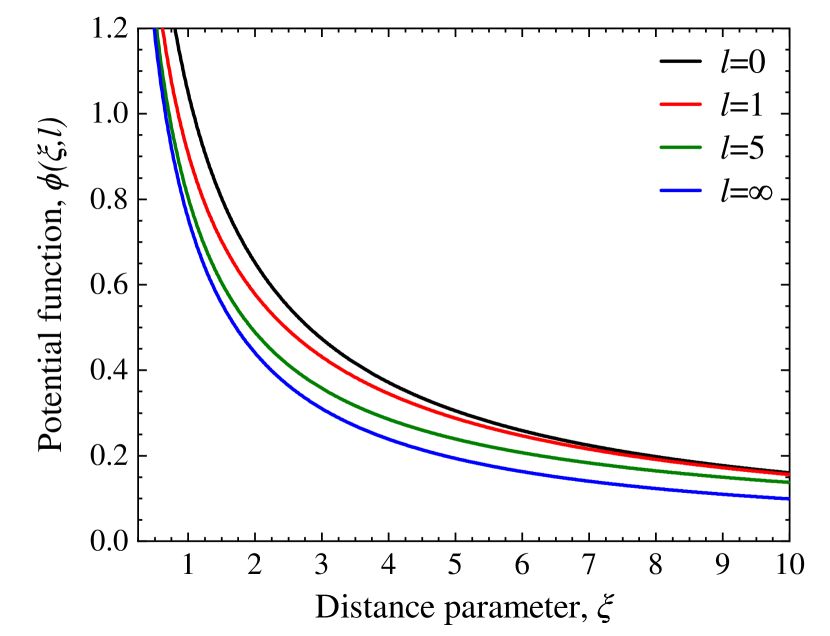
Figure 3: Potential function $\phi(\xi,l)$ for four values of dimensionless length parameter, $l$: $l$=0, $l$=1, $l$=5, and $l$=$\infty$ as a function of a dimensionless distance parameter, $\xi$.

The evolution of the $\phi(\xi,l)$ potential as a function of a $\xi$ parameter is presented in Fig. 3 for four $l$ values. As can be seen in the Figure, the strongest $\phi(\xi,l)$ potential is apparent for $l=0$, while the weakest potential is for the case $l=\infty$, the potential for $l>0$ lies in the region in between of two former potentials. The obtained results are in full agreement with the previously reported results [21, 9, 26], where it was shown that an increase in the average dielectric constant of the media surrounding the ML leads to a decrease in the confining potential.

IV Excitonic spectrum in non-homogeneous system

Using the $\phi(\xi,l)$ potential, expressed by Eq. (25), we can evaluate the energy spectrum of excitons in the investigated structure composed of S-TMD ML as a function of the parameter $l$. The corresponding equation for eigenvalues is given by

$$\Big{[}b^{2}\frac{1}{\xi}\frac{d}{d\xi}\Big{(}\xi\frac{d}{d\xi}\Big{)}+2b\phi(\xi,l)+\epsilon\Big{]}\psi(\xi)=0,$$ (28)

where we introduced $b=\hbar^{2}\varepsilon_{\text{hBN}}^{2}/(\mu e^{2}r_{0})$ and $E=Ry^{*}\epsilon$. $Ry^{*}=\mu e^{4}/(2\hbar^{2}\varepsilon_{\text{hBN}}^{2})$ is an effective Rydberg energy and $\psi(\xi)$ represents the wave function of an exciton. $\mu=m_{e}m_{h}/(m_{e}+m_{h})$ is the reduced mass of the exciton ($e$-$h$ pair) with the effective electron ($m_{e}$) and hole ($m_{h}$) masses and $e$ represents electron’s charge.

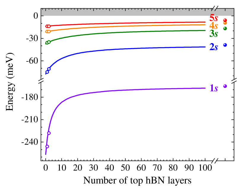
Figure 4: Energy spectrum of $s$ excitonic state in the WSe₂ ML encapsulated in hBN layers as a function of the thickness of the top hBN layer (colored online). The full points correspond to the case of a semi-infinite thickness of top hBN. The colored open points represent the energy spectrum of excitons calculated individually for the mono- and bilayer top hBN (see SM for details). Note that the thickness of the bottom hBN layer is semi-infinite in both cases. The gray-shaded region represents the infinity of states above the bandgap energy.

Let us examine the case of WSe₂ ML with $r_{0}=4.5$ nm [38] and $\mu=0.21\,m_{0}$ [6], where $m_{0}$ is electron’s mass. It gives $b\approx 1.13357$ and $Ry^{*}\approx 141$ meV. For the WSe₂ ML $r_{0}=4.5$ nm, the dimensionless parameter $l$ corresponds to the $l$ nm of the thickness of the top flake of hBN. Taking into account that the distance between the layers in hBN (in other words, the thickness of hBN ML) is $d=0.33$ nm [42], we conclude that $l=1$ corresponds to 3 layers of hBN.

Note that in the case of the few-layer top hBN flake, when its discreteness can play an important role, the phenomenological continuous model of the hBN medium considered here should be additionally verified. To do it, we perform separately the numerical analysis for the ML and BL of the top hBN in the Supplementary Material (SM).

The calculated energy spectra of an exciton for the ground (1$s$) and four excited (2$s$ – 5$s$) states as a function of the thickness of the top hBN layer for the aforementioned continuous model as well as the discrete one for the thinnest layers are presented in Fig. 4. Due to the observed evolutions in the Figure, three main points can be raised: (i) the continuous model provides a very good method for calculating the exciton spectrum, even in the case of the extremely thin top hBN flake of about 1-2 layers; The largest discrepancy is observed between the homogeneous model and the ML of top hBN for the energy of 1$s$ state of about 5$\%$. (ii) the energies of excitonic states are subjected to the most significant variations for the thinnest top hBN layers with thicknesses below about 30 layers. For thicker top hBN layers, the corresponding excitonic energies are almost fixed; (iii) the thickness effect of the top hBN layer is the largest for the ground 1$s$ state of the exciton with its substantial reduction when the number of excitonic states is increased. The maximum change of the 1$s$ energy of about 91 meV between two limits: without the top hBN layer and with its infinite thickness. The analogous differences of the 2$s$, 3$s$, 4$s$, and 5$s$ states are of the order of 39 meV, 20 meV, 13 meV, and 8 meV, respectively.

Table 1: Calculated binding energies of excitons ($E_{\mathrm{b}}$) in WSe₂ ML encapsulated in hBN layers for selected numbers of the top hBN layer.

Number of
top hBN layers	0	3	6	10	20	40	100	$\infty$
$E_{\mathrm{b}}$ (meV)	256	212	197	187	177	172	168	165

We can focus on analyzing the excitonic binding energy ($E_{\mathrm{b}}$, defined as the energy difference between the electronic bang gap and the ground 1$s$ state. The dependence of the $E_{\mathrm{b}}$ energy in the WSe₂ ML encapsulated in the hBN layers for selected numbers of the top hBN layer is summarized in Table 1. The experimentally measured binding energies of excitons in WSe₂ MLs encapsulated in hBN flakes is of about 170 meV [9, 5, 6, 7]. Besides the structures with the hBN encapsulation investigated experimentally differ from the one analyzed in this work, $e.g.$, a WSe₂ ML sandwiched between 10 nm thick hBN deposited on the core of a single-mode optical fiber [9], the theoretically calculated binding energies are in very good agreement with the experimental ones. Using our approach, the excitonic binding energy can be changed by almost 40% in the transition from the sample without the top hBN layer ($E_{\mathrm{b}}$=256 meV) to the one with the infinite thickness of the top hBN layer ($E_{\mathrm{b}}$=165 meV). This reveals that the thickness of the surrounding media of S-TMD MLs also plays a crucial role in the modification of the exciton energy spectrum in S-TMD MLs in addition to the engineering of the surrounding dielectric environment, $i.e.$, the encapsulation of an ML in media characterized by dielectric constants [21].

To fulfill our results we consider two additional cases which can be realized in the experiment: i) the case of the SiO₂ substrate, $i.e.$, $\varepsilon_{1}=2.1$; ii) the case of the suspended S-TMD monolayer together with the thick hBN flake, $i.e.$, $\varepsilon_{1}=1$. We repeat the calculation of the exciton spectrum in the S-TMD monolayer for both cases and compare them with the previous results in the SM. Finally, we study the general case, presented by Eq. (20), with a non-zero distance gap $\delta$ between the S-TMD monolayer and the sub- and superstrate, see SM for details.

V Summary

We obtained the generalization of the Rytova-Keldysh potential for the heterostructures which consists of the substrate, the monolayer S-TMD, the top hBN flake of finite thickness, and the overtop superstrate. Using the analytical interpretation of the potential, we calculated the energy spectrum of the excitonic states in the S-TMD monolayer placed on a semi-infinite hBN substrate and covered with a top hBN layer with thickness $L$. We presented that the binding energies of the excitons can be significantly modified due to screening effects and as a function of thickness $L$. For WSe₂ ML in such a structure, we demonstrated that the energies of the excitonic states are substantially adjusted for the thinnest top hBN layers with thicknesses below about 30 layers. For the thickness of the top layer larger than 30 layers, the binding energies of the excitons saturate to the excitons energies in the bulk hBN case.

Additionally, we have found that the thickness effect of the top hBN layer is the largest for the ground 1$s$ state of the exciton. It results in a significant reduction in excitonic binding energy that can be changed by almost 40% in the transition from the sample without the top hBN layer to the one with an infinite thickness of the top hBN layer. The proposed model may be applicable to other 2D layered materials in which the screening effects on the excitonic spectrum play an essential role, $e.g.$, 2D perovskites [43].

VI Acknowledgments

The work has been supported by the National Science Centre, Poland (grant no. 2018/31/B/ST3/02111) and by the Czech Science Foundation (project GA23-06369S).

SI The modified Rytova-Keldysh potential for the case of ultrathin top hBN flake

In our study, we modeled the top layer of hBN with its thickness $L$ and the macroscopic in- ($\varepsilon_{\text{hBN},\parallel}$) and out-of-plane ($\varepsilon_{\text{hBN},\perp}$) dielectric constants of hBN, $i.e.$, in the limit of the continuous hBN medium. However, in the case of the ultrathin top hBN flake, where it consists of only a few layers of hBN monolayers, the use of such a limit is doubtful. In order to find the limits of applicability of the continuous model, we derive the modified Rytova-Keldysh potential with a few layers of the hBN.

To do it, we consider the modification of the system studied in the main text. The bottom semi-infinite substrate remains unchanged. Thus, it is characterized by in- ($\varepsilon_{1,\parallel}$) and out-of-plane ($\varepsilon_{1,\perp}$) dielectric constants and occupies the domain $z\in]-\infty,-\delta]$. The S-TMD monolayer is placed in the plane $z=0$ with its in-plane polarizability $\chi_{\text{TMD}}$. The first top hBN flake consists of $N$ layer and has a thickness $L=Nd$. Here $d=0.33$  nm is the distance between the hBN layers in a bulk hBN crystal. The $j$th layer of the hBN flake is placed in the $z_{j}=jd$ plane. Each hBN layer is characterized by the in-plane polarizability $\chi_{\text{hBN}}$. The second top layer with the in- ($\varepsilon_{3,\parallel}$) and out-of-plane ($\varepsilon_{3,\perp}$) dielectric constants occupies the domain $z\in[L+\delta,\infty[$.

In order to find the potential energy between two charges in the S-TMD monolayer, we solve the following electrostatic problem. We consider the point-like charge $Q$ at the point $(0,0,z^{\prime})$, where $0<z^{\prime}\neq z_{j}<L$ and calculate the potential in such a system following [36]. Similarly to the previous case, we consider 3 regions: bottom semi-infinite medium with the potential $\Phi_{1}(\bm{\rho},z)$, second top semi-infinite layer with the potential $\Phi_{3}(\bm{\rho},z)$, and the space between them with the potential $\Phi_{2}(\bm{\rho},z)$, where we introduced the in-plane vector $\bm{\rho}=(x,y)$. Using the cylindrical symmetry of the problem, we present the potentials in the form

$$\Phi_{j}(\bm{\rho},z)=\frac{1}{(2\pi)^{2}}\int d^{2}\mathbf{k}e^{i\mathbf{k}\bm{\rho}}\Phi_{j}(\mathbf{k},z)$$ (29)

The Maxwell’s equation $\text{div}\,\mathbf{D}_{1,3}=0$ for 1-st and 3-rd regions ($j=1,3$) reads

$$-\varepsilon_{j,\parallel}\mathbf{k}^{2}\Phi_{j}(\mathbf{k},z)+\varepsilon_{j,\perp}\frac{d^{2}\Phi_{j}(\mathbf{k},z)}{dz^{2}}=0.$$ (30)

The solutions to these equations are

$$\Phi_{1}(\mathbf{k},z) =Ae^{\kappa_{1}z}, \,z\in]-\infty,-\delta],$$ for (31)

$$\Phi_{3}(\mathbf{k},z) =Be^{-\kappa_{3}z}, \,z\in[L+\delta,\infty[,$$ for (32)

where $\kappa_{j}=|\mathbf{k}|\sqrt{\varepsilon_{j,\parallel}/\varepsilon_{j,\perp}}=k\sqrt{\varepsilon_{j,\parallel}/\varepsilon_{j,\perp}}$.

The equation for the potential $\Phi_{2}(\mathbf{r},z)$ takes the form

$$\Delta_{\parallel}\Phi_{2}(\bm{\rho},z)+ \epsilon_{\perp}\frac{d^{2}\Phi_{2}(\bm{\rho},z)}{dz^{2}}=$$

$$-4\pi[Q\delta(\bm{\rho})\delta(z-z^{\prime})-\varrho_{\text{ind}}(\bm{\rho},z)],$$ (33)

where $\Delta_{\parallel}$ is 2D Laplace operator. We introduced the out-of-plane dielectric constant ($\epsilon_{\perp}$) of the hBN flake with $N>1$. In the case $N=1$, one needs to put $\epsilon_{\perp}=1$. The first term on the right-hand side of the equation is the charge density of the charge $Q$. The second term $\varrho_{\text{ind}}(\bm{\rho},z)$ represents the induced charge density due to the polarization of the hBN and S-TMD layer by charge $Q$. Following Ref. [36], we present the induced charge in the form

$$\varrho_{\text{ind}}(\bm{\rho},z)=- \chi_{\text{hBN}}\sum_{j=1}^{N}\delta(z-z_{j})\Delta_{\parallel}\Phi_{2}(\bm{\rho},z_{j})-$$

$$- \chi_{\text{TMD}}\delta(z)\Delta_{\parallel}\Phi_{2}(\bm{\rho},0).$$ (34)

Using the Fourier transform (29) of the potential $\Phi_{2}(\bm{\rho},z)$ we present Eq. (SI) as

$$\Big{[}\mathbf{k}^{2}-\epsilon_{\perp}\frac{d^{2}}{dz^{2}}\Big{]}\Phi_{2}(\mathbf{k},z)= 4\pi Q\delta(z-z^{\prime})-2r_{0}k^{2}\delta(z)\Phi_{2}(\mathbf{k},0)$$

$$- 2R_{0}k^{2}\sum_{j=1}^{N}\delta(z-z_{j})\Phi_{2}(\mathbf{k},z_{j}),$$ (35)

where we introduced the in-plane screening lengths $r_{0}=2\pi\chi_{\text{TMD}}$ and $R_{0}=2\pi\chi_{\text{hBN}}$ for S-TMD and hBN monolayers, respectively. Integrating this equation in the regions $z\in[-\epsilon,\epsilon]$, $z\in[z_{j}-\epsilon,z_{j}+\epsilon]$, and $z\in[z^{\prime}-\epsilon,z^{\prime}+\epsilon]$ one obtains the following conditions in the limit $\epsilon\rightarrow 0$

$$\epsilon_{\perp}\frac{d\Phi_{2}(\mathbf{k},z)}{dz}\Big{|}^{+0}_{-0} =2r_{0}k^{2}\Phi_{2}(\mathbf{k},0),$$ (36)

$$\epsilon_{\perp}\frac{d\Phi_{2}(\mathbf{k},z)}{dz}\Big{|}^{z_{j}+0}_{z_{j}-0} =2R_{0}k^{2}\Phi_{2}(\mathbf{k},z_{j}),$$ (37)

$$\epsilon_{\perp}\frac{d\Phi_{2}(\mathbf{k},z)}{dz}\Big{|}^{z^{\prime}+0}_{z^{\prime}-0} =-4\pi Q.$$ (38)

At the points $z\neq 0\,,z_{j}\,,z^{\prime}$ the Eq. (SI) is simplified

$$\Big{[}\mathbf{k}^{2}-\epsilon_{\perp}\frac{d^{2}}{dz^{2}}\Big{]}\Phi_{2}(\mathbf{k},z)=0$$ (39)

Therefore, the general solution for $\Phi_{2}(\mathbf{k},z)$ can be written in the form

$$\Phi_{2}(\mathbf{k},z)= \Psi_{0}e^{-K|z-z^{\prime}|}+\sum_{j=1}^{N}\Psi_{j}e^{-K|z-z_{j}|}+$$

$$+ \Psi e^{-K|z|}+\alpha e^{Kz}+\beta e^{-Kz},$$ (40)

where $\Psi_{0}$,$\Psi_{j}$,$\Psi$, $\alpha$ and $\beta$ are unknown functions of $K=k/\sqrt{\epsilon_{\perp}}$. The aforementioned boundary conditions together with the equation give the following restrictions

$$\Psi= -r_{0}K\Phi_{2}(\mathbf{k},0),$$

$$\Psi_{j}= -R_{0}K\Phi_{2}(\mathbf{k},z_{j}),$$

$$\Psi_{0}= 2\pi Q/\epsilon_{\perp}K.$$ (41)

Considering the boundary conditions for the electrostatic potential and for the out-of-plane component of the displacement field at $z=-\delta$

$$\Phi_{1}(\mathbf{k},-\delta) =\Phi_{2}(\mathbf{k},-\delta),$$ (42)

$$\frac{\varepsilon_{1,\perp}}{\epsilon_{\perp}}\frac{d\Phi_{1}(\mathbf{k},z)}{dz}\Big{|}_{z=-\delta} =\frac{d\Phi_{2}(\mathbf{k},z)}{dz}\Big{|}_{z=-\delta},$$ (43)

and at $z=L+\delta$

$$\Phi_{3}(\mathbf{k},L+\delta) =\Phi_{2}(\mathbf{k},L+\delta),$$ (44)

$$\frac{\varepsilon_{3,\perp}}{\epsilon_{\perp}}\frac{d\Phi_{3}(\mathbf{k},z)}{dz}\Big{|}_{z=L+\delta} =\frac{d\Phi_{2}(\mathbf{k},z)}{dz}\Big{|}_{z=L+\delta},$$ (45)

we get the following equations

$$Ae^{-\kappa_{1}\delta}=\Psi_{0}e^{-K(z^{\prime}+\delta)}+\sum_{j=1}^{N}\Psi_{j}e^{-K(z_{j}+\delta)}+\Psi e^{-K\delta}+\alpha e^{-K\delta}+\beta e^{K\delta},$$ (46)

$$A\frac{\varepsilon_{1}}{\sqrt{\epsilon_{\perp}}}e^{-\kappa_{1}\delta}=\Psi_{0}e^{-K(z^{\prime}+\delta)}+\sum_{j=1}^{N}\Psi_{j}e^{-K(z_{j}+\delta)}+\Psi e^{-K\delta}+\alpha e^{-K\delta}-\beta e^{K\delta},$$ (47)

$$Be^{-\kappa_{3}(L+\delta)}=\Psi_{0}e^{-K(L+\delta-z^{\prime})}+\sum_{j=1}^{N}\Psi_{j}e^{-K(L+\delta-z_{j})}+\Psi e^{-K(L+\delta)}+\alpha e^{K(L+\delta)}+\beta e^{-K(L+\delta)},$$ (48)

$$B\frac{\varepsilon_{3}}{\sqrt{\epsilon_{\perp}}}e^{-\kappa_{3}(L+\delta)}=\Psi_{0}e^{-K(L+\delta-z^{\prime})}+\sum_{j=1}^{N}\Psi_{j}e^{-K(L+\delta-z_{j})}+\Psi e^{-K(L+\delta)}-\alpha e^{K(L+\delta)}+\beta e^{-K(L+\delta)}.$$ (49)

where we introduced the short notation $\varepsilon_{j}=\sqrt{\varepsilon_{j,\perp}\varepsilon_{j,\parallel}}$ for $j=1,3$. Introducing $a=\varepsilon_{1}/\sqrt{\epsilon_{\perp}}$ and $b=\varepsilon_{3}/\sqrt{\epsilon_{\perp}}$, and considering the general case $a,b\neq 1$ we remove the parameters $A$ and $B$ from the above equations and obtain

$$\Psi_{0}e^{-K(z^{\prime}+\delta)}+\sum_{j=1}^{N}\Psi_{j}e^{-K(z_{j}+\delta)}+\Psi e^{-K\delta}+\alpha e^{-K\delta}+\Big{(}\frac{a+1}{a-1}\Big{)}\beta e^{K\delta}=0,$$ (50)

$$\Psi_{0}e^{-K(L+\delta-z^{\prime})}+\sum_{j=1}^{N}\Psi_{j}e^{-K(L+\delta-z_{j})}+\Psi e^{-K(L+\delta)}+\Big{(}\frac{b+1}{b-1}\Big{)}\alpha e^{K(L+\delta)}+\beta e^{-K(L+\delta)}=0.$$ (51)

Note that the solution of the aforementioned system of equations for the case $a=1$ and/or $b=1$ can be obtained from the general solution by taking the corresponding limit.

We solve the general equation in a few steps. First, we write the system of equations in the following form

$$e^{-K\delta}\alpha+\Big{(}\frac{a+1}{a-1}\Big{)}e^{K\delta}\beta= \mathcal{A},$$

$$\Big{(}\frac{b+1}{b-1}\Big{)}e^{K(L+\delta)}\alpha+e^{-K(L+\delta)}\beta= \mathcal{B},$$ (52)

where we introduced the following notations $\mathcal{A}=-\Psi_{0}e^{-K(z^{\prime}+\delta)}-\sum_{j=1}^{N}\Psi_{j}e^{-K(z_{j}+\delta)}-\Psi e^{-K\delta}$, $\mathcal{B}=-\Psi_{0}e^{-K(L+\delta-z^{\prime})}-\sum_{j=1}^{N}\Psi_{j}e^{-K(L+\delta-z_{j})}-\Psi e^{-K(L+\delta)}$. Solving the system of equations (SI) one gets

$$\alpha=\frac{\mathcal{A}e^{-K(L+\delta)}-\mathcal{B}\Big{(}\frac{a+1}{a-1}\Big{)}e^{K\delta}}{D},$$ (53)

$$\beta=\frac{\mathcal{B}e^{-K\delta}-\mathcal{A}\Big{(}\frac{b+1}{b-1}\Big{)}e^{K(L+\delta)}}{D},$$ (54)

with $D=e^{-K(L+2\delta)}-\Big{(}\frac{a+1}{a-1}\Big{)}\Big{(}\frac{b+1}{b-1}\Big{)}e^{K(L+2\delta)}$. Substituting these solutions into (SI), we express $\Phi_{2}(\mathbf{k},z)$ via $N+2$ parameters $\Psi_{0}$, $\Psi_{j}$ and $\Psi$. Then, using the latter expression, we calculate the expressions for the potential in $z=0$, $z=z^{\prime}$, and $z=z_{l},\,l=1,2\dots N$ points

$$\Phi_{2}(\mathbf{k},0)= \Psi_{0}e^{-Kz^{\prime}}+\sum_{j=1}^{N}\Psi_{j}e^{-Kz_{j}}+\Psi+\alpha+\beta,$$

$$\Phi_{2}(\mathbf{k},z^{\prime})= \Psi_{0}+\sum_{j=1}^{N}\Psi_{j}e^{-K(z_{l}-z^{\prime})}+\Psi e^{-Kz^{\prime}}+\alpha e^{Kz^{\prime}}+\beta e^{-Kz^{\prime}},$$

$$\Phi_{2}(\mathbf{k},z_{l})= \Psi_{0}e^{-K(z_{l}-z^{\prime})}+\sum_{j=1}^{N}\Psi_{j}e^{-K|z_{l}-z_{j}|}+\Psi e^{-Kz_{l}}+\alpha e^{Kz_{l}}+\beta e^{-Kz_{l}},$$ (55)

which together with (SI) gives the complete set of equations for the parameters $\Psi_{0}$, $\Psi_{j}$, and $\Psi$. In the system of Eqs. (SI), we considered the particular case $0<z^{\prime}<z_{1}<z_{2}<\dots<z_{N}=L$ for simplicity. Then we simplify our solutions by taking the following limits $\delta\rightarrow 0$ and $z^{\prime}\rightarrow 0$, and obtain $\Phi_{2}(\mathbf{k},z=0)=(2\pi Q/k)v(k)$ which defines the electrostatic potential $\Phi(\rho)$ in the S-TMD plane, which reads

$$\Phi(\rho)=Q\int_{0}^{\infty}dkJ_{0}(k\rho)v(k).$$ (56)

We derive the expressions for the case of monolayer ($v_{\text{m}}$) and bilayer ($v_{\text{b}}$) hBN flake to demonstrate the aforementioned algorithm and then estimate the spectrum of excitons for both cases.

First, we consider the case of monolayer hBN, $i.e.$, $N=1$, $\epsilon_{\perp}=1$, and hence $a=\varepsilon_{1}$, $b=\varepsilon_{3}$ and $K=k$. Following the procedure mentioned above, we obtain the result for the monolayer (m)

$$v_{\text{m}}(k)=\frac{1-\left(\frac{2kR_{0}+\varepsilon_{3}-1}{2kR_{0}+\varepsilon_{3}+1}\right)e^{-2dk}}{(kr_{0}+\frac{\varepsilon_{1}+1}{2})-(kr_{0}+\frac{\varepsilon_{1}-1}{2})\left(\frac{2kR_{0}+\varepsilon_{3}-1}{2kR_{0}+\varepsilon_{3}+1}\right)e^{-2dk}}.$$ (57)

Note that this result looks similar to the general result in the main text (see Eq. 23). The eigenvalue problem for this potential has a form

$$\Big{[}\widetilde{b}^{2}\frac{1}{\xi}\Big{(}\xi\frac{d}{d\xi}\Big{)}+2\widetilde{b}\int_{0}^{\infty}dxJ_{0}(x\xi)v_{\text{m}}(x)+\epsilon\Big{]}\psi(\xi)=0.$$ (58)

Here $v_{\text{m}}(x=kr_{0})\equiv v_{\text{m}}(k)$, $\epsilon=E/Ry$ and $\xi=\rho/r_{0}$ are the dimensionless energy and coordinate, respectively, with $Ry=\mu e^{4}/2\hbar^{2}$ and $\widetilde{b}=\hbar^{2}/(\mu e^{2}r_{0})$. To calculate the spectrum of excitons, we consider the particular case $\varepsilon_{1}=\varepsilon_{\text{hBN}}=4.5$, $\varepsilon_{3}=1$. Using formula (4) from Ref. [38] and in-plane dielectric constant of the monolayer hBN $\varepsilon_{\text{hBN},\parallel}=4.98$ from [44] $R_{0}=(\varepsilon_{\text{hBN},\parallel}-1)d/2$, we obtain $R_{0}=6.57\,\mbox{\AA}$. Note that this screening length is much smaller than, for example, in the WSe₂ monolayer $r_{0}=45\,\mbox{\AA}$ [38]. Solving the eigenvalue equation with $\widetilde{b}\approx 0.056$ and taking into account that $Ry=2.856$ eV we obtain the following binding energies: $E_{1}\approx-246$ meV, $E_{2}\approx-75$ meV, $E_{3}\approx-36$ meV, $E_{4}\approx-21$ meV, $E_{5}\approx-14$ meV. Note that this result is close to the result of the homogeneous model proposed in the main text: $E_{1}\approx-235$ meV, $E_{2}\approx-73$ meV, $E_{3}\approx-36$ meV, $E_{4}\approx-21$ meV, $E_{5}\approx-14$ meV. The main difference between the two calculated spectra is the binding energy of the $1s$ exciton. The smaller binding energy of the $1s$ state in the homogeneous model can be explained by the less effective screening of the Coulomb potential than in the model considered here.

The potential for the case of the bilayer flake $N=2$ $\Phi_{2}(\mathbf{k},z=0)=(2\pi Q/k\sqrt{\epsilon_{\perp}})v_{\text{b}}(k)$ with the corresponding out-of-plane dielectric constant $\epsilon_{\perp}$ is

$$v_{\text{b}}(k)=\frac{1-\frac{2KR_{0}(b+2KR_{0})}{(KR_{0}+1)(b+2KR_{0}+1)}e^{-2dK}+\frac{(KR_{0}-1)(b+2KR_{0}-1)}{(KR_{0}+1)(b+2KR_{0}+1)}e^{-4dK}}{\frac{a+1}{2}+Kr_{0}-\frac{[(a+2Kr_{0})(b+2KR_{0})-1]}{(KR_{0}+1)(b+2KR_{0}+1)}KR_{0}e^{-2dK}+\frac{(KR_{0}-1)(b+2KR_{0}-1)}{(KR_{0}+1)(b+2KR_{0}+1)}\left(\frac{a-1}{2}+Kr_{0}\right)e^{-4dK}}.$$ (59)

Here $K=k/\sqrt{\epsilon_{\perp}}$, $a=\varepsilon_{1}/\sqrt{\epsilon_{\perp}}$, and $b=\varepsilon_{3}/\sqrt{\epsilon_{\perp}}$. The eigenvalue problem for the case of the bilayer reads

$$\Big{[}\widetilde{b}^{2}\epsilon_{\perp}\frac{1}{\xi}\Big{(}\xi\frac{d}{d\xi}\Big{)}+2\widetilde{b}\int_{0}^{\infty}dxJ_{0}(x\xi)v_{\text{b}}(x)+\epsilon\Big{]}\psi(\xi)=0.$$ (60)

Here $v_{\text{b}}(x=kr_{0}/\sqrt{\epsilon_{\perp}})\equiv v_{\text{b}}(k)$, $\epsilon=E/Ry$ and $\xi=\rho\sqrt{\epsilon_{\perp}}/r_{0}$ are the dimensionless energy and coordinate, respectively, with $Ry=\mu e^{4}/2\hbar^{2}$ and $\widetilde{b}=\hbar^{2}/(\mu e^{2}r_{0})$. For the numerical estimation of the exciton spectrum in this case, we use $\varepsilon_{1}=4.5$ and $\varepsilon_{3}=1$ and the result of Ref. [44] for $\epsilon_{\perp}=2.91$. The spectrum of the excitons then reads $E_{1}\approx-228$ meV, $E_{2}\approx-71$ meV, $E_{3}\approx-35$ meV, $E_{4}\approx-21$ meV, $E_{5}\approx-14$ meV. It is surprisingly very close to the result of the homogeneous model, described in the main text, $E_{1}\approx-221$ meV, $E_{2}\approx-70$ meV, $E_{3}\approx-35$ meV, $E_{4}\approx-21$ meV, $E_{5}\approx-14$ meV. Therefore, we conclude that the homogeneous model provides a very good method for calculating the exciton spectrum, even in the case of an extremely thin top hBN flake of about 1-2 layers.

SII Effective Coulomb potential in the S-TMD flake of finite thickness

We consider a suspended multilayer crystal of S-TMD as a set of $N$ layers of S-TMD, arranged in parallel to the $xy$ plane. The position of $j$-th layer is defined by the coordinate $z_{j}$. We arrange the layers in the following way $0<z_{1}<z_{2}<\dots z_{N}<L$. As in the previous case, we suppose that a multilayer is polarized in the in-plane direction, with the 2D susceptibility $\chi_{\text{TMD}}=r_{0}/2\pi$. The out-of-plane polarization of the S-TMD crystal is $\epsilon_{\perp}$.

The electric potential $\Phi(\bm{\rho},z)$ for the point-like charge $Q$ at the point $\mathbf{r}=(0,0,z^{\prime})$ of multilayer reads

$$\Big{[}\Delta_{\parallel}+\epsilon_{\perp}\frac{d^{2}}{dz^{2}}\Big{]}\Phi(\bm{\rho},z)= -4\pi Q\delta(\bm{\rho})\delta(z-z^{\prime})-$$

$$- 2r_{0}\sum_{j=1}^{N}\delta(z-z_{j})\Delta_{\parallel}\Phi(\bm{\rho},z_{j}).$$ (61)

This equation can be solved with the help of Fourier transform

$$\Phi(\bm{\rho},z)=\frac{1}{(2\pi)^{3}}\int d^{2}\mathbf{k}\int_{-\infty}^{\infty}dq\,e^{i\mathbf{k}\bm{\rho}+iqz}\Phi(\mathbf{k},q).$$ (62)

After substitution it into the main equation one gets

$$[k^{2}+\epsilon_{\perp}q^{2}]\Phi(\mathbf{k},q)=4\pi Qe^{-iqz^{\prime}}-2r_{0}k^{2}\sum_{j=1}^{N}e^{-iqz_{j}}\Phi(\mathbf{k},z_{j}),$$ (63)

where

$$\Phi(\mathbf{k},z_{j})=\frac{1}{2\pi}\int_{-\infty}^{\infty}dqe^{iqz_{j}}\Phi(\mathbf{k},q).$$ (64)

Note that a solution of this equation can be found in the $N\rightarrow\infty$ limit, $i.e.$, the case of the infinite (bulk) S-TMD crystal. To do it we rewrite the finite sum in the equation in the form

$$\lim_{N\rightarrow\infty}\sum_{j=1}^{N}e^{-iqz_{j}}\Phi(\mathbf{k},z_{j})=\frac{1}{d}\Phi(\mathbf{k},q).$$ (65)

Here, we used the parametrization $z_{j}=A+d(j-1)$ with $d=(B-A)/(N-1)$, with $A/B$ as the coordinate of the bottom/top layer of the multilayer, $d$ is the distance between layers in the crystal. To obtain the aforementioned result we present the sum in the form

$$\sum_{j=1}^{N}e^{i(q^{\prime}-q)z_{j}}=e^{i(q^{\prime}-q)\frac{(B+A)}{2}}\frac{\sin\Big{[}\frac{(q^{\prime}-q)}{2}dN\Big{]}}{\sin\Big{[}\frac{(q^{\prime}-q)}{2}d\Big{]}},$$ (66)

then considering $(q^{\prime}-q)dN/2\sim 1$, $(q^{\prime}-q)d/2\sim 1/N$, and using

$$\lim_{N\rightarrow\infty}\frac{\sin\Big{[}\frac{(q^{\prime}-q)}{2}dN\Big{]}}{\Big{[}\frac{(q^{\prime}-q)}{2}d\Big{]}}=\pi\delta\Big{[}\frac{(q^{\prime}-q)}{2}d\Big{]},$$ (67)

we obtain

$$\lim_{N\rightarrow\infty}\sum_{j=1}^{N}e^{i(q^{\prime}-q)z_{j}}=\pi\delta\Big{[}\frac{(q^{\prime}-q)}{2}d\Big{]}.$$ (68)

Then one can rewrite the Eq. (63) in the form

$$\Big{[}\Big{(}1+2\frac{r_{0}}{d}\Big{)}k^{2}+\epsilon_{\perp}q^{2}\Big{]}\Phi(\mathbf{k},q)=4\pi Qe^{-iqz^{\prime}}.$$ (69)

This result coincides with the equation for the potential of charge $Q$, placed in the point $z^{\prime}$ for the crystal with the in-plane $\varepsilon_{\parallel}=1+2r_{0}/d$ and out-of-plane $\varepsilon_{\perp}=\epsilon_{\perp}$ dielectric constants, see [38].

To find the solution of Eq. (63) for the finite number of layers $N$ we divide it on $[\mathbf{k}^{2}+\epsilon_{\perp}q^{2}]$, integrate over $q$ with additional $e^{iqz_{m}}$ function, evaluate the integral

$$\int_{-\infty}^{\infty}dq\frac{e^{iqz}}{k^{2}+\epsilon_{\perp}q^{2}}=\frac{\pi}{k\sqrt{\epsilon_{\perp}}}e^{-k|z|/\sqrt{\epsilon_{\perp}}}.$$ (70)

and obtain the following system of equations for variables $\Phi(\mathbf{k},z_{j})$

$$\sum_{j=1}^{N}\left[\delta_{mj}+\frac{kr_{0}}{\sqrt{\epsilon_{\perp}}}e^{-k\frac{|z_{m}-z_{j}|}{\sqrt{\epsilon_{\perp}}}}\right]\Phi(\mathbf{k},z_{j})=\frac{2\pi Q}{k\sqrt{\epsilon_{\perp}}}e^{-k\frac{|z_{m}-z^{\prime}|}{\sqrt{\epsilon_{\perp}}}}.$$ (71)

This system of the linear equation can be solved analytically for small values of the number of layers $N\sim 1$. The solution for the larger numbers $N\gg 1$ can be done numerically. The obtained expressions for the potentials in the $z_{j}$th layer $\Phi(\mathbf{k},z_{j})$ are needed to evaluate the effective Coulomb interaction between the electron and hole localized in the corresponding layers, see Ref. [39].

The alternative way to find the solution of Eq. (63) is to present it in the form of an integral equation

$$\Phi(\mathbf{k},q)=\frac{2\pi Qe^{-iqz^{\prime}}}{k^{2}+\epsilon_{\perp}q^{2}}-\int_{-\infty}^{\infty}dq^{\prime}f(q,q^{\prime})\Phi(\mathbf{k},q^{\prime}),$$ (72)

with the kernel

$$f(q,q^{\prime})=\frac{r_{0}k^{2}}{k^{2}+\epsilon_{\perp}q^{2}}\frac{1}{\pi}\sum_{j=1}^{N}e^{-i(q-q^{\prime})z_{j}},$$ (73)

valid for any distribution of the coordinates $z_{j}$.

SIII Spectrum of excitons for the different cases of the substrate

We evaluate the energy spectrum of excitons in the investigated structure for the case of different substrates as a function of the parameter $l$. The eigenvalues equation reads

$$\Big{[}b^{2}\frac{1}{\xi}\frac{d}{d\xi}\Big{(}\xi\frac{d}{d\xi}\Big{)}+2b\phi(\xi,l,\varepsilon_{1})+\epsilon\Big{]}\psi(\xi)=0,$$ (74)

where we introduced $b=\hbar^{2}\varepsilon_{\text{hBN}}^{2}/(\mu e^{2}r_{0})$ and $E=Ry^{*}\epsilon$ with $Ry^{*}=\mu e^{4}/(2\hbar^{2}\varepsilon_{\text{hBN}}^{2})$, as in the main text. Here $\psi(\xi)$ represents the wave function of an exciton in terms of dimensionless coordinate $\xi=\rho\varepsilon_{\text{hBN}}/r_{0}$. The dimensionless potential function $\phi(\xi,l,\varepsilon_{1})$ has a form

$$\phi(\xi,l,\varepsilon_{1})=\int_{0}^{\infty}dx\frac{J_{0}(x\xi)\Big{[}1+\frac{\varepsilon_{\text{hBN}}-1}{\varepsilon_{\text{hBN}}+1}\exp\Big{(}-2\sqrt{\frac{\varepsilon_{\text{hBN},\parallel}}{\varepsilon_{\text{hBN},\perp}}}xl\Big{)}\Big{]}}{x+\frac{\varepsilon_{\text{hBN}}+\varepsilon_{1}}{2\varepsilon_{\text{hBN}}}+\Big{[}x+\frac{\varepsilon_{1}-\varepsilon_{\text{hBN}}}{2\varepsilon_{\text{hBN}}}\Big{]}\frac{\varepsilon_{\text{hBN}}-1}{\varepsilon_{\text{hBN}}+1}\exp\Big{(}-2\sqrt{\frac{\varepsilon_{\text{hBN},\parallel}}{\varepsilon_{\text{hBN},\perp}}}xl\Big{)}}.$$ (75)

As one can see for $\varepsilon_{1}=\varepsilon_{\text{hBN}}$, it coincides with the previously obtained result, $i.e.$, $\phi(\xi,l,\varepsilon_{\text{hBN}})=\phi(\xi,l)$, as should be.

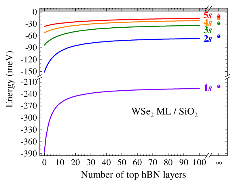
Figure S1: Energy spectrum of $s$ excitonic state in the WSe₂ ML deposited on SiO₂ substrate and covered with top hBN layer as a function of its thickness. The gray-shaded region represents the infinity of states above the bandgap energy.

Table 2: Calculated binding energies of excitons ($E_{\mathrm{b}}$) in the WSe₂ ML placed on the SiO₂ substrate and covered with top hBN layer for selected numbers of the top hBN layer.

Number of
top hBN layers	0	3	6	10	20	40	100	$\infty$
$E_{\mathrm{b}}$ (meV)	386	310	281	263	245	234	226	220

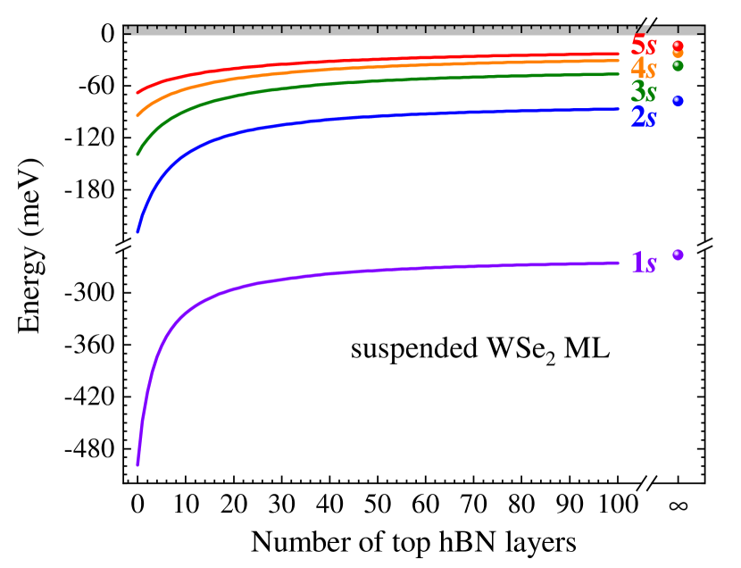
Figure S2: Energy spectrum of $s$ excitonic state in the suspended WSe₂ ML covered with top hBN layer as a function of its thickness. The gray-shaded region represents the infinity of states above the bandgap energy.

Table 3: Calculated binding energies of excitons ($E_{\mathrm{b}}$) in the suspended WSe₂ ML covered with top hBN layer for selected numbers of the top hBN layer.

Number of
top hBN layers	0	3	6	10	20	40	100	$\infty$
$E_{\mathrm{b}}$ (meV)	499	391	350	324	296	278	266	256

We solve the eigenvalue equation for the case of SiO₂ substrate, $\varepsilon_{1}=2.1$ [20] and for the case of suspended S-TMD monolayer, $\varepsilon_{1}=1$. The calculated energy spectra of an exciton for the ground (1$s$) and four excited (2$s$ $-$ 5$s$) states as a function of the thickness of the top hBN layer for the case of the SiO₂ substrate and of the suspended S-TMD monolayer are shown in Figs. S1 and S2, respectively. The corresponding dependences of the excitonic binding energy ($E_{b}$, defined as the energy difference between the electronic bang gap and the ground 1$s$ state) in the WSe₂ ML for the case of the SiO₂ substrate and of the suspended S-TMD monolayer are summarized Tables 2 and 3.

SIV Spectrum of excitons for the case of the non-zero distance between monolayer and sub- and superstrate

Let us consider the general case of the S-TMD monolayer encapsulated in between different media, presented in Fig. 3 of the main text. In this scenario the $k$-depended, and, hence, $\rho$-dependent, effective in-plane Coulomb potential depends on three distance parameters: the screening length in the plane of the S-TMD monolayer $r_{0}$, the thickness of the top flake $L$, and the distance $\delta$ between the monolayer and the substrate (the same distance is between the monolayer and the top flake). As a result, the shape of the Coulomb potential is modified, providing the three-parametric spectrum and wave functions of the excitons. It makes their general analytical consideration quite tricky. However, some conclusions can be made by studying the limit cases $\delta\rightarrow 0$, $\delta\rightarrow\infty$, $L\rightarrow 0$, etc.

The limit $\delta\rightarrow 0$ is considered in the main text, where it was demonstrated that the spectrum depends on the dimensionless parameter $L/r_{0}$. One can conclude that a similar answer can be obtained for small $\delta\ll r_{0},L$. The typical scale of binding energies of the excitons $E_{\text{b}}$ is suppressed by the dielectric constants of the surrounding media: $E_{\text{b}}\propto Ry/(\varepsilon_{1}+\varepsilon_{3})^{2}$ for $L\rightarrow 0$, and $E_{\text{b}}\propto Ry/(\varepsilon_{1}+\varepsilon_{2})^{2}$ for $L\rightarrow\infty$, see Ref. [45] for details. The opposite limit $\delta\rightarrow\infty$ corresponds to the case of the suspended monolayer, with the dielectric function $\varepsilon(k)=kr_{0}+1$. Therefore, the scale of the binding energies of excitons is $E_{\text{b}}\propto Ry$. The intermediate case, where $\delta\sim r_{0},L$, interpolates between the two aforementioned limits. Therefore, for fixed parameters $r_{0},L$, the binding energies are increasing with the increasing $\delta$, see also Ref. [30].

In order to demonstrate the impact of this parameter on the excitons’ spectrum in such a system, we consider the WSe₂ monolayer, encapsulated in hBN medium, with $\delta=5\,\mbox{\AA}$, as an example. The corresponding eigenvalue equation has a form

$$\Big{[}b^{2}\frac{1}{\xi}\frac{d}{d\xi}\Big{(}\xi\frac{d}{d\xi}\Big{)}+2b\phi(\xi,l,\eta)+\epsilon\Big{]}\psi(\xi)=0,$$ (76)

where $l=\varepsilon_{\text{hBN}}L/r_{0}$, $\eta=\varepsilon_{\text{hBN}}\delta/r_{0}$, $b=\hbar^{2}\varepsilon_{\text{hBN}}^{2}/(\mu e^{2}r_{0})$, $E=Ry^{*}\epsilon$, $Ry^{*}=\mu e^{4}/(2\hbar^{2}\varepsilon_{\text{hBN}}^{2})$. The dimensionless potential function has a form

$$\phi(\xi,l,\eta)=\int_{0}^{\infty}dxJ_{0}(x\xi)/\varepsilon(x,l,\eta),$$ (77)

with the $\eta$-dependent dielectric function

$$\varepsilon(x,l,\eta)=x+\frac{1-\alpha^{2}\exp[-4x\eta]-\alpha^{2}(1-\exp[-4x\eta])\exp\big{[}-2\sqrt{\frac{\varepsilon_{\text{hBN},\parallel}}{\varepsilon_{\text{hBN},\perp}}}x(l-\eta)\big{]}}{\varepsilon_{\text{hBN}}(1-\alpha\exp[-2x\eta])(1-\alpha\exp[-2x\eta]+\alpha(\exp[-2x\eta]-\alpha)\exp\big{[}-2\sqrt{\frac{\varepsilon_{\text{hBN},\parallel}}{\varepsilon_{\text{hBN},\perp}}}x(l-\eta)\big{]})},$$ (78)

and $\alpha=(\varepsilon_{\text{hBN}}-1)/(\varepsilon_{\text{hBN}}+1)$. The calculated spectrum, as a function of the number of the layers of the top hBN layer, is presented in Fig. S3. The corresponding dependence of the $E_{b}$ energy is summarized Table 4.

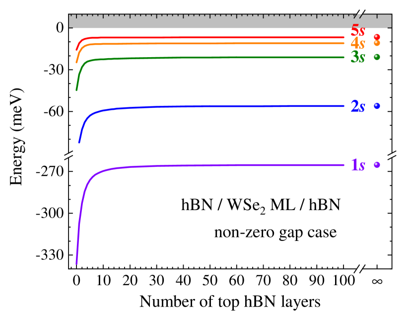
Figure S3: Energy spectrum of $s$ excitonic state in the hBN-encapsulated WSe₂ ML covered with top hBN layer as a function of its thickness for the non-zero distance, $\delta=5\,\mbox{\AA}$, between the ML and sub- and superstrate. The gray-shaded region represents the infinity of states above the bandgap energy.

Table 4: Calculated binding energies of excitons ($E_{\mathrm{b}}$) in the hBN-encapsulated WSe₂ ML covered with top hBN layer as a function of the number of layers of the top hBN layer for the non-zero distance between the ML and sub- and superstrate, $\delta=5\,\mbox{\AA}$.

Number of
top hBN layers	0	3	6	10	20	40	100	$\infty$
$E_{\mathrm{b}}$ (meV)	336	284	274	270	267	266	265	265

One can see that the obtained excitonic ladder for the relatively large parameter $\delta$ deviates significantly from the ladder obtained in the main text ($\delta=0$). This conclusion is valid also for the general case, presented in Fig. 3 of the main text. It provides us with the instrument for the analysis of the spectrum in realistic heterostructures. Namely, knowing the parameters of the system, one can first calculate the spectrum for the case of $\delta=0$ (provided in the main text). If the calculated spectrum significantly deviates from the experimentally observed excitonic ladder, one concludes that there is a non-zero distance gap between the layers, and the more general model, with $\delta>0$, should be considered.

References

- Cheiwchanchamnangij and Lambrecht [2012] T. Cheiwchanchamnangij and W. R. L. Lambrecht, Phys. Rev. B 85, 205302 (2012).
- Ramasubramaniam [2012] A. Ramasubramaniam, Phys. Rev. B 86, 115409 (2012).
- Qiu et al. [2013] D. Y. Qiu, F. H. da Jornada, and S. G. Louie, Phys. Rev. Lett. 111, 216805 (2013).
- Liu et al. [2019] E. Liu, J. van Baren, T. Taniguchi, K. Watanabe, Y.-C. Chang, and C. H. Lui, Phys. Rev. B 99, 205420 (2019).
- Chen et al. [2019] S.-Y. Chen, Z. Lu, T. Goldstein, J. Tong, A. Chaves, J. Kunstmann, L. S. R. Cavalcante, T. Woźniak, G. Seifert, D. R. Reichman, T. Taniguchi, K. Watanabe, D. Smirnov, and J. Yan, Nano Letters 19, 2464 (2019).
- Molas et al. [2019a] M. R. Molas, A. O. Slobodeniuk, K. Nogajewski, M. Bartos, L. Bala, A. Babiński, K. Watanabe, T. Taniguchi, C. Faugeras, and M. Potemski, Phys. Rev. Lett. 123, 136801 (2019a).
- Kapuściński et al. [2021] P. Kapuściński, A. Delhomme, D. Vaclavkova, A. O. Slobodeniuk, M. Grzeszczyk, M. Bartos, K. Watanabe, T. Taniguchi, C. Faugeras, and M. Potemski, Communications Physics 4, 186 (2021).
- Sell et al. [2022] J. C. Sell, J. R. Vannucci, D. G. Suárez-Forero, B. Cao, D. W. Session, H.-J. Chuang, K. M. McCreary, M. R. Rosenberger, B. T. Jonker, S. Mittal, and M. Hafezi, Phys. Rev. B 106, L081409 (2022).
- Stier et al. [2018] A. V. Stier, N. P. Wilson, K. A. Velizhanin, J. Kono, X. Xu, and S. A. Crooker, Phys. Rev. Lett. 120, 057405 (2018).
- Goryca et al. [2019] M. Goryca, J. Li, A. V. Stier, T. Taniguchi, K. Watanabe, E. Courtade, S. Shree, C. Robert, B. Urbaszek, X. Marie, and S. A. Crooker, Nature Communications 10, 4172 (2019).
- Arora et al. [2019] A. Arora, T. Deilmann, T. Reichenauer, J. Kern, S. Michaelis de Vasconcellos, M. Rohlfing, and R. Bratschitsch, Phys. Rev. Lett. 123, 167401 (2019).
- Chernikov et al. [2014] A. Chernikov, T. C. Berkelbach, H. M. Hill, A. Rigosi, Y. Li, O. B. Aslan, D. R. Reichman, M. S. Hybertsen, and T. F. Heinz, Phys. Rev. Lett. 113, 076802 (2014).
- Gerber et al. [2019] I. C. Gerber, E. Courtade, S. Shree, C. Robert, T. Taniguchi, K. Watanabe, A. Balocchi, P. Renucci, D. Lagarde, X. Marie, and B. Urbaszek, Phys. Rev. B 99, 035443 (2019).
- Ye et al. [2014] Z. Ye, T. Cao, K. O’Brien, H. Zhu, X. Yin, Y. Wang, S. G. Louie, and X. Zhang, Nature 513, 214 (2014).
- He et al. [2014] K. He, N. Kumar, L. Zhao, Z. Wang, K. F. Mak, H. Zhao, and J. Shan, Phys. Rev. Lett. 113, 026803 (2014).
- Wang et al. [2015] G. Wang, X. Marie, I. Gerber, T. Amand, D. Lagarde, L. Bouet, M. Vidal, A. Balocchi, and B. Urbaszek, Phys. Rev. Lett. 114, 097403 (2015).
- Kusaba et al. [2021] S. Kusaba, Y. Katagiri, K. Watanabe, T. Taniguchi, K. Yanagi, N. Naka, and K. Tanaka, Opt. Express 29, 24629 (2021).
- MacDonald and Ritchie [1986] A. H. MacDonald and D. S. Ritchie, Phys. Rev. B 33, 8336 (1986).
- Koteles and Chi [1988] E. S. Koteles and J. Y. Chi, Phys. Rev. B 37, 6332 (1988).
- Stier et al. [2016] A. V. Stier, N. P. Wilson, G. Clark, X. Xu, and S. A. Crooker, Nano Letters 16, 7054 (2016).
- Raja et al. [2017] A. Raja, A. Chaves, J. Yu, G. Arefe, H. M. Hill, A. F. Rigosi, T. C. Berkelbach, P. Nagler, C. Schüller, T. Korn, C. Nuckolls, J. Hone, L. E. Brus, T. F. Heinz, D. R. Reichman, and A. Chernikov, Nature Communications 8, 15251 (2017).
- Hsu et al. [2019] W.-T. Hsu, J. Quan, C.-Y. Wang, L.-S. Lu, M. Campbell, W.-H. Chang, L.-J. Li, X. Li, and C.-K. Shih, 2D Materials 6, 025028 (2019).
- Riis-Jensen et al. [2020] A. C. Riis-Jensen, M. N. Gjerding, S. Russo, and K. S. Thygesen, Phys. Rev. B 102, 201402 (2020).
- Bieniek et al. [2022] M. Bieniek, K. Sadecka, L. Szulakowska, and P. Hawrylak, Nanomaterials 12, 1582 (2022).
- Shi et al. [2022] J. Shi, Z. Lin, Z. Zhu, J. Zhou, G. Q. Xu, and Q.-H. Xu, ACS Nano 16, 15862 (2022).
- Nguyen-Truong [2022] H. T. Nguyen-Truong, Phys. Rev. B 105, L201407 (2022).
- Gerber and Marie [2018] I. C. Gerber and X. Marie, Phys. Rev. B 98, 245126 (2018).
- Latini et al. [2015] S. Latini, T. Olsen, and K. S. Thygesen, Phys. Rev. B 92, 245123 (2015).
- Rösner et al. [2016] M. Rösner, C. Steinke, M. Lorke, C. Gies, F. Jahnke, and T. O. Wehling, Nano Letters 16, 2322 (2016).
- Florian et al. [2018] M. Florian, M. Hartmann, A. Steinhoff, J. Klein, A. W. Holleitner, J. J. Finley, T. O. Wehling, M. Kaniber, and C. Gies, Nano Letters 18, 2725 (2018).
- Andersen et al. [2015] K. Andersen, S. Latini, and K. S. Thygesen, Nano Letters 15, 4616 (2015).
- Van Tuan et al. [2018] D. Van Tuan, M. Yang, and H. Dery, Phys. Rev. B 98, 125308 (2018).
- Ajayi et al. [2017] O. A. Ajayi, J. V. Ardelean, G. D. Shepard, J. Wang, A. Antony, T. Taniguchi, K. Watanabe, T. F. Heinz, S. Strauf, X.-Y. Zhu, and J. C. Hone, 2D Materials 4, 031011 (2017).
- Cadiz et al. [2017] F. Cadiz, E. Courtade, C. Robert, G. Wang, Y. Shen, H. Cai, T. Taniguchi, K. Watanabe, H. Carrere, D. Lagarde, M. Manca, T. Amand, P. Renucci, S. Tongay, X. Marie, and B. Urbaszek, Phys. Rev. X 7, 021026 (2017).
- Wierzbowski et al. [2017] J. Wierzbowski, J. Klein, F. Sigger, C. Straubinger, M. Kremser, T. Taniguchi, K. Watanabe, U. Wurstbauer, A. W. Holleitner, M. Kaniber, K. Müller, and J. J. Finley, Scientific Reports 7, 12383 (2017).
- Cudazzo et al. [2011] P. Cudazzo, I. V. Tokatly, and A. Rubio, Phys. Rev. B 84, 085406 (2011).
- Keldysh [1979] L. V. Keldysh, JETP Lett. 29, 716 (1979).
- Berkelbach et al. [2013] T. C. Berkelbach, M. S. Hybertsen, and D. R. Reichman, Phys. Rev. B 88, 045318 (2013).
- Kipczak et al. [2023] L. Kipczak, A. O. Slobodeniuk, T. Woźniak, M. Bhatnagar, N. Zawadzka, K. Olkowska-Pucko, M. Grzeszczyk, K. Watanabe, T. Taniguchi, A. Babiński, and M. R. Molas, 2D Materials 10, 025014 (2023).
- Rytova [1967] N. S. Rytova, Moscow University Physics Bulletin 3, 30 (1967).
- Steinhoff et al. [2018] A. Steinhoff, T. O. Wehling, and M. Rösner, Phys. Rev. B 98, 045304 (2018).
- Xu et al. [2015] B. Xu, M. Lv, X. Fan, W. Zhang, Y. Xu, and T. Zhai, Integrated Ferroelectrics 162, 85 (2015).
- Baranowski and Plochocka [2020] M. Baranowski and P. Plochocka, Advanced Energy Materials 10, 1903659 (2020).
- Laturia et al. [2018] A. Laturia, , M. L. Van de Put, and W. G. Vandenberghe, npj 2D Materials and Applications 2, 6 (2018).
- Molas et al. [2019b] M. R. Molas, A. O. Slobodeniuk, T. Kazimierczuk, K. Nogajewski, M. Bartos, P. Kapuściński, K. Oreszczuk, K. Watanabe, T. Taniguchi, C. Faugeras, P. Kossacki, D. M. Basko, and M. Potemski, Phys. Rev. Lett. 123, 096803 (2019b).
Supplementary Material for "Exciton spectrum in atomically thin monolayers: