Probing the structural evolution along the fission path in the superheavy nucleus ²⁵⁶Sg

Abstract

The evolution of structure property along the fission path in the superheavy nucleus ²⁵⁶Sg is predicted through the multi-dimensional potential-energy(or Routhian)-surface calculations, in which the phenomenological deformed Woods-Saxon potential is adopted. Calculated nuclear deformations and fission barriers for ${}^{256}_{106}$Sg₁₅₀ and its neighbors, e.g., ^258,260Sg, ²⁵⁴Rf and ²⁵²No are presented and compared with other theoretical results. A series of energy maps and curves are provided and used to evaluate the corresponding shape-instability properties, especially in the directions of triaxial $\gamma$ and different hexadecapole deformations (e.g., $\alpha_{40}$, $\alpha_{42}$ and $\alpha_{44}$). It is found that the triaxial deformation may help the nucleus bypass the first fission-barrier of the axial case. After the first minimum in the nuclear energy surface, the fission pathway of the nucleus can be affected by $\gamma$ and hexadecapole deformation degrees of freedom. In addition, microscopic single-particle structure, pairing and Coriolis effects are briefly investigated and discussed.

Keywords: structure evolution, fission path; fission barrier; superheavy nuclei; macroscopic-microscopic model.

1. Introduction

The evolution of nuclear structure properties with some degree of freedom (e.g., nucleon number, spin, temperature, etc) is one of the most significant issues in nuclear physics Voigt1983 , especially towards the superheavy mass region. Great progress has been made in the synthesis of superheavy nuclei with the development of the radioactive beam facility, heavy-ion accelerator and highly-effective detector systems Liu2011 ; Zhao2011 ; Oganessian2015 . Spontaneous fission is usually one of important decay modes in a superheavy nucleus and the barrier along the fission path is critical to understand the fission process Abusara2010 ; Kostryukov2021 . For instance, the survival probability of a synthesized superheavy nucleus in the heavy-ion fusion reaction is directly related to such a barrier, during the cooling process of a compound nucleus, which plays a decisive role in the competition between nucleon evaporation and fission (a small change of the fission barrier may result in several orders of magnitude difference in survival probability) Lu2014 . Nevertheless, it is still rather difficult to give an accurate description for the fission barrier so far. To a large extent, the barrier size and shape can be determined by the fission path in the nuclear energy surface.

Up to now, there are several types of models which are widely used for investigating nuclear fission phenomena, including e.g., the macroscopic-microscopic (MM) models  Moller2009 ; Kowal2010 ; Moller2015 ; Gaamouci2021 ; Dong2015 , the nonrelativistic energy density functionals based on zero-range Skyrme and finite-range Gogny interactions  Bender1998 ; Bonneau2004 ; Staszczak2009 ; Staszczak2007 ; Ling2020 ; Chen2022 , the extended Thomas-Fermi plus Strutinsky integral methods Dutta2000 ; Mamdouh2001 , and the covariant density functional theory Abusara2010 ; Li2010 ; Ring2011 . The MM methods usually have the high descriptive power as well as simplicity of calculation and thus are still used by many researchers so far. In such an approach, the empirical one-body nuclear mean-filed (e.g., the Nilsson and Woods-Saxon potentials) Hamiltonian is used to solve the microscopic single-particle levels and wave functions and a macroscopic liquid-drop model (e.g., the standard liquid-drop model Myers1966 , the finite-range droplet model Moller1988 , and the Lublin-Strasboug drop model Pomorski2003 , etc) is combined to describe the nuclear bulk property. In recent years, the model parameters, including their uncertainties and propagations, in both phenomenological Woods-Saxon potential and the macroscopic liquid-drop model are still studied and optimized, e.g., cf Refs. Zhang2021 ; Dedes2019 ; Meng2022cpc ; Meng2022 ; Gaamouci2021 ; Yang2022 . Indeed, the parameters of MM models are mainly from the fitting of available single-particle levels of several spherical nuclei and several thousand nuclear-mass data. They are generally successful near the $\beta$-stability line, especially in the medium and heavy nuclear regions. Without the preconceived knowledge, e.g., about the measured densities and single-particle energies, it may be needed to test whether the modeling and model parameters of a phenomenological one-body potential are still valid enough. Part of our aim of this work is to test the theoretical method in such aspects.

Prior to this work, 16 Sg isotopes from $A=258$ to 273 were synthesized by the fusion-evaporation reactions, e.g., ²³⁸U(³⁰Si,$xn$)^268-xSg NNDC2022 . It was reported that the lightest even-even Sg isotope, ²⁵⁸Sg, has a revised half-life of $2.8^{+0.8}_{-0.5}$ $ms$ Heberger1997 . Naturally, one expects that based on the fusion-evaporation mechanism, the superheavy nuclide ²⁵⁶Sg will be synthesized as the next candidate which is the nearest even-even nucleus to the known ones in this isotopic chain. Keeping this in mind, we predict the properties of structure evolution along the possible fission path for the superheavy nuclide ²⁵⁶Sg in this project. In our previous studies, we systematically investigated the octupole correlation properties for 42 even-even nuclei with $102\leq Z\leq 112$ Wang2012 and the triaxial effects on the inner fission barriers in 95 tranuranium even-even nuclei $94\leq Z\leq 118$ Chai2018 . The triaxiality and Coriolis effects on the fission barrier in isovolumic nuclei with $A=256$ were investigated, where the ²⁵⁶Sg was calculated but just focused on the first (inner) fission barrier Chai2018a . In Ref. Chai2019CTP , we investigated the effects of various deformations (e.g., $\beta_{2}$, $\gamma$ and $\beta_{4}$) on the first barrier in even-even nuclei with $N=152$ and $94\leq Z\leq 108$. In addition, we studied the collective rotational effects including the $\alpha$-decay-chain nuclei (from ²¹⁶Po and ²⁷²Cn) Chai2018IJMPE and ^254-258Rf Wang2014 by the similar calculation. The primary purpose of this study is to investigate the effects of different deformation parameters, especially the axial and non-axial hexadepole deformations, on the fission path of ²⁵⁶Sg by analyzing the topography of the energy surfaces calculated in a reasonable subspace of collective coordinates (it is impossible to calculate in the full deformation space). The probe of the shape evolution along the fission path on the energy landscape will be useful for understanding the formation mechanism of the fission barrier. We provide the analysis of the single-particle structures, shell and pairing evolutions, especially at the minima and saddles. Sobiczewski et al Sobiczewski2010 systematically investigated the static inner barrier of heaviest nuclei with proton number $98\leq Z\leq 126$ and neutron number $134\leq N\leq 192$ in a multidimensional deformation space and pointed out that the inclusion of the non-axial hexadecapole shapes lowers the barrier by up to about 1.5 MeV. In the synthesis of the superheavy nuclei, nuclear hexadecapole deformations were revealed to have an important influence on production cross sections of superheavy nuclei by e.g., affecting the driving potentials and the fusion probabilities Wang2010 ; Bao2016 .

This paper is organized as follows: In Sect.2, we briefly describe the outline of the theoretical framework and the details of the numerical calculations. The results of the calculations and their relevant discussion are given in Sect.3. Finally, the concluding remarks will be given in Sect.4.

2. Theoretical framework

In what follows, we recall the unified procedure and give the necessary references related to the present theoretical calculation, which may be somewhat helpful for some readers to clarify some details (e.g., the various variants of the pairing-energy contribution within the framework of the macroscopic-microscopic method). We employ potential-energy(or Routhian)-surface calculation to study the present project. This method is based on the macroscopic-microscopic model Moller1995 ; Werner1992 and the cranking approximation Inglis1954 ; Inglis1955 ; Inglis1956 , which is one of widely used and powerful tools in nuclear structure research, especially for rotating nuclei. The usual expression for the total energy in the rotating coordinate frame (namely, the so-called total Routhian) reads Nazarewicz1989

$$E^{\omega}(Z,N,\hat{\beta}) = E^{\omega}_{macr}(Z,N,\hat{\beta})+\delta E^{\omega}_{micro}(Z,N,\hat{\beta}),$$ (1)

where $E^{\omega}(Z,N,\hat{\beta})$ represents the total Routhian of a nucleus ($Z$, $N$) at frequency $\omega$ and deformation $\hat{\beta}$. The first term on the right-hand side in Eq. (1) denotes the macroscopic (liquid drop, or LD) energy with the rigid-body moment of inertia calculated classically at a given deformation, assuming a uniform density distribution; $\delta E^{\omega}_{micro}$ represents the contribution due to the microscopic effects under rotation. After rearrangement employing elementary transformations Bengtsson1975 ; Werner1995 ; Neergard1975 ; Neergard1976 ; Andersson1976 , the total Routhian can be rewritten as,

$$E^{\omega}(Z,N,\hat{\beta}) = E^{\omega=0}(Z,N,\hat{\beta})$$ (2)

$$+ [\langle\hat{H}^{\omega}(Z,N,\hat{\beta})\rangle-\langle\hat{H}^{\omega=0}(Z,N,\hat{\beta})\rangle]$$

$$- \frac{1}{2}\omega^{2}[\mathcal{J}_{macr}(A,\hat{\beta})-\mathcal{J}_{Stru}(Z,N,\hat{\beta})].$$

The notations for the quantities in Eq. (2) are standard Nazarewicz1989 ; Satula1994NPA . The term $E^{\omega=0}(Z,N,\hat{\beta})$ is the static total energy (corresponding $\omega=0$) which consists of a macroscopic LD part $E_{LD}(Z,N,\hat{\beta})$ and a shell correction $\delta E_{shell}(Z,N,\hat{\beta})$ and a pairing-energy contribution $\delta E_{pair}(Z,N,\hat{\beta})$ (neglecting the superscript $\omega=0$) . The second term in the square brackets represents the energy change of the cranked Hamiltonian $\hat{H}^{\omega}(Z,N,\hat{\beta})$ due to rotation Nazarewicz1989 ; Satula1994NPA . In Eq. (2), it is usually and reasonably assumed that the average pairing energy of the liquid-drop term and the Strutinsky-smeared pairing energy cancel each other Nazarewicz1989 . Therefore, one can further write Eq. (2) as [cf. Ref. Dudek1988 and references therein],

$$E^{\omega}(Z,N,\hat{\beta}) = E_{LD}(Z,N,\hat{\beta})$$ (3)

$$+ \delta E_{shell}(Z,N,\hat{\beta})+\delta E_{pair}(Z,N,\hat{\beta})$$

$$+ [\langle\hat{H}^{\omega}(Z,N,\hat{\beta})\rangle-\langle\hat{H}^{\omega=0}(Z,N,\hat{\beta})\rangle].$$

As known, several phenomenological LD models (such as standard liquid drop model Myers1966 , finite-range droplet model Moller1995 , Lublin-Strasbourg drop model Pomorski2003 ) with slight difference have been developed for calculating the smoothly varying part. In these LD models, the dominating terms are mainly associated with the volume energy, the surface energy and the Coulomb energy. In the present work, the macroscopic energy is given by the standard LD model with the parameters used by Myers and Swiatecki Myers1966 .

The single-particle levels used below are calculated by solving numerically the Schrödinger equation with the Woods-Saxon (WS) Hamiltonian Dudek1980

$$H_{WS} = T+V_{\rm cent}(\vec{r};\hat{\beta})+V_{\rm so}(\vec{r},\vec{p},\vec{s};\hat{\beta})$$ (4)

$$+V_{\rm Coul}(\vec{r},\hat{\beta}),$$

where the Coulomb potential $V_{\rm Coul}(\vec{r},\hat{\beta})$ defined as a classical electrostatic potential of a uniformly charged drop is added for protons. The central part of the WS potential is calculated as

$$V_{\rm cent}(\vec{r},\hat{\beta})=\frac{V_{0}[1\pm\kappa(N-Z)/(N+Z)]}{1+\exp[\text{dist}_{\Sigma}(\vec{r},\hat{\beta})/a]},$$ (5)

where the plus and minus signs hold for protons and neutrons, respectively and the parameter $a$ denotes the diffuseness of the nuclear surface. The term $\text{dist}_{\Sigma}(\vec{r},\hat{\beta})$ represents the distance of a point $\vec{r}$ from the nuclear surface $\Sigma$ parameterized in term of the multipole expansion of spherical harmonics $Y_{\lambda\mu}(\theta,\phi)$ (which are convenient to describe the geometrical properties), that is,

$$\Sigma:R(\theta,\phi)=r_{0}A^{1/3}c(\hat{\beta})\Big{[}1+\sum_{\lambda}\sum_{\mu=-\lambda}^{+\lambda}\alpha_{\lambda\mu}Y^{*}_{\lambda\mu}(\theta,\phi)\Big{]},$$ (6)

where the function $c(\hat{\beta})$ ensures the conservation of the nuclear volume with a change in the nuclear shape and $\hat{\beta}$ denotes the set of all the deformation parameters $\{\alpha_{\lambda\mu}\}$. For a given nucleus with mass number $A$, a limiting value of $\lambda<A^{1/3}$ is often estimated. In the present shape parametrization, we consider quadrupole and hexadecapole degrees of freedom, including nonaxial deformations, namely, $\hat{\beta}$ $\equiv$ $\{\alpha_{20}$, $\alpha_{2\pm 2}$, $\alpha_{40}$, $\alpha_{4\pm 2}$, $\alpha_{4\pm 4}\}$. The quantity $R(\theta,\phi)$ denotes the distance of any point on the nuclear surface from the origin of the coordinate system. Because only the even $\lambda$ and even $\mu$ components are taken into account, the present parametrisation will preserve three symmetry planes. After requesting the hexadecpole degrees of freedom to be functions of the scalars in the quadrupole tensor $\alpha_{2\mu}$, one can reduce the number of independent coefficients to three, namely, $\beta_{2}$, $\gamma$ and $\beta_{4}$, which obey the relationships Bhagwat2010

$$\left\{\begin{array}[]{lcl}\alpha_{20}=\beta_{2}\cos\gamma\\[5.69054pt] \alpha_{22}=\alpha_{2-2}=-\frac{1}{\sqrt{2}}\beta_{2}\sin\gamma\\[5.69054pt] \alpha_{40}=\frac{1}{6}\beta_{4}(5\cos^{2}\gamma+1)\\[5.69054pt] \alpha_{42}=\alpha_{4-2}=-\frac{1}{12}\sqrt{30}\beta_{4}\sin 2\gamma\\[5.69054pt] \alpha_{44}=\alpha_{4-4}=\frac{1}{12}\sqrt{70}\beta_{4}\sin^{2}\gamma.\\[5.69054pt] \end{array}\right.$$ (7)

The ($\beta_{2},\gamma,\beta_{4}$) parametrization has all the symmetry properties of Bohr’s ($\beta_{2},\gamma$) parametrization Bohr1952 . The spin-orbit potential, which can strongly affects the level order, is defined by

$$V_{\rm so}(\vec{r},\vec{p},\vec{s};\hat{\beta}) = -\lambda\Big{[}\frac{\hbar}{2mc}\Big{]}^{2}$$

$$\times \bigg{\{}\nabla\frac{V_{0}[1\pm\kappa(N-Z)/(N+Z)]}{1+exp[dist_{\Sigma_{so}}(\vec{r},\hat{\beta})/a_{so}]}\bigg{\}}\times\vec{p}\cdot\vec{s},$$

where $\lambda$ denotes the strength parameter of the effective spin-orbit force acting on the individual nucleons. The new surface $\Sigma_{so}$ is different from the one in Eq. (6) due to the different radius parameter. In the present work, the WS parameters are taken from Refs. Bhagwat2010 ; Meng2018 , as listed in Table 1.

Table 1: The adopted WS parameters for both protons and neutrons (for more details, cf e.g, Ref. Bhagwat2010 ). Note that nuclear shape does not sensitively depend on the parameter sets in well-deformed nuclei, especially those with large stiffness.

V0 (MeV)		$\kappa$		r0 (fm)		$a$(fm)		$\lambda$		(r0)so (fm)		$a_{\rm so}$ (fm)
53.754		0.791		1.190		0.637		29.494		1.190		0.637

In computing the Woods-Saxon Hamiltonian matrix, the eigenfunctions of the axially deformed harmonic oscillator potential in the cylindrical coordinate system are adopted as the basis functions Cwiok1987 ,

$$|n_{\rho}n_{z}\Lambda\Sigma\rangle=\psi_{n_{\rho}}^{\Lambda}(\rho)\psi_{n_{z}}(z)\psi_{\Lambda}(\varphi)\chi(\Sigma),$$ (9)

where

$$\left\{\begin{array}[]{lcl}\psi_{n_{\rho}}^{\Lambda}(\rho)&=&\frac{\sqrt{n_{\rho}!}}{\sqrt{(n_{\rho}+|\Lambda|)!}}(2m\omega_{\rho}/\hbar)^{1/2}\\ &&\times e^{-\frac{\eta^{2}}{2}}\eta^{\Lambda}L_{n_{\rho}}^{|\Lambda|}(\eta),\\[5.69054pt] \psi_{n_{z}}(z)&=&\frac{1}{\sqrt{\sqrt{\pi}2^{n_{z}}n_{z}!}}(2m\omega_{z}/\hbar)^{1/4}\\ &&\times e^{-\frac{\xi^{2}}{2}}H_{n_{z}}(\xi),\\[5.69054pt] \psi_{\Lambda}(\varphi)&=&\frac{1}{\sqrt{2\pi}}e^{i\Lambda\varphi},\\[5.69054pt] \end{array}\right.$$ (10)

and $\chi(\Sigma)$ represents the spin wave functions, cf. e.g., Sec. 3.1 in Ref. Cwiok1987 for more details. In our calculation, the eigenfunctions with the principal quantum number $N\leq$ 12 and 14 have been chosen as a basis for protons and neutrons, respectively. It is found that, by such a basis cutoff, the results are sufficiently stable with respect to a possible enlargement of the basis space. In addition, the time reversal (resulting in the Kramers degeneracy) and spatial symmetries (e.g., the existence of three symmetry $x-y$, $y-z$ and $z-x$ planes) are used for simplifying the Hamiltonian matrix calculation.

The shell correction $\delta E_{shell}(Z,N,\hat{\beta})$, as seen in Eq. (3), is usually the most important correction to the LD energy. Strutinsky first proposed a phenomenological expression,

$$\delta E_{shell}(Z,N,\hat{\beta})=\sum e_{i}-\int e\tilde{g}(e)de,$$ (11)

where $e_{i}$ denotes the calculated single-particle levels and $\tilde{g}(e)$ is the so-called smooth level density. Obviously, the smooth level distribution function is the most important quantity, which was early defined as,

$$\tilde{g}(e,\gamma)\equiv\frac{1}{\gamma\sqrt{\pi}}\sum_{i}{\rm exp}[-\frac{(e-e_{i})^{2}}{\gamma^{2}}],$$ (12)

where $\gamma$ indicates the smoothing parameter without much physical significance. To eliminate any possibly strong $\gamma$-parameter dependence for the final result, the mathematical form of the smooth level density $\tilde{g}(e)$ has been optimized by introducing a phenomenological curvature-correction polynomial $P_{p}(x)$Werner1995 ; Nilsson1969 ; Strutinsky1975 ; Ivanyuk1978 . Then, the $\tilde{g}(e)$ expression will take the form

$$\tilde{g}(e,\gamma,p)=\frac{1}{\gamma\sqrt{\pi}}\sum_{i=1}P_{p}(\frac{e-e_{i}}{\gamma})\times{\rm exp}[-\frac{(e-e_{i})^{2}}{\gamma^{2}}],$$ (13)

where the corrective polynomial $P_{p}(x)$ can be expanded in terms of the Hermite or Laguerre polynomials. The corresponding coefficients of the expansion can be obtained by using the orthogonality properties of these polynomials and Strutinsky condition (i.e., see the APPENDIX in Ref.Pomorski2004 ). In fact, this method can be considered standard so far. For instance, the integration in Eq. (12) can be calculated as follows (see Ref.Bolsterli1972 for more details),

$$\int e\tilde{g}(e,\gamma,p)de = \int\tilde{e}(n)dn$$ (14)

$$= \sum_{i=1}\{\frac{1}{2}e_{i}[1+{\rm erf}(\frac{\tilde{\lambda}-e_{i}}{\gamma})]$$

$$-\frac{1}{2\sqrt{\pi}}\gamma{\rm exp}[-\frac{(\tilde{\lambda}-e_{i})^{2}}{\gamma^{2}}]$$

$$-\frac{1}{\sqrt{\pi}}{\rm exp}[-\frac{(\tilde{\lambda}-e_{i})^{2}}{\gamma^{2}}]$$

$$\times\sum_{m=1}^{p}c_{m}[\frac{1}{2}\gamma H_{m}(\frac{\tilde{\lambda}-e_{i}}{\gamma})$$

$$+e_{i}H_{m-1}(\frac{\tilde{\lambda}-e_{i}}{\gamma})$$

$$+m\gamma H_{m-2}(\frac{\tilde{\lambda}-e_{i}}{\gamma})]\}.$$

Of course, there are some other methods developed for the shell correction calculations, e.g., the semiclassical Wigner-Kirkwood expansion method Vertse1998 ; Bhagwat2010 and the Green’s function method Kruppa2000 . In this work, the widely used Strutinsky method is adopted though its known problems which appear for mean-field potentials of finite depth as well as for nuclei close to the proton or neutron drip lines. The smooth density is calculated with a sixth-order Hermite polynomial and a smoothing range $\gamma=1.20\hbar\omega_{0}$, where $\hbar\omega_{0}=41/A^{1/3}$ MeV, indicating a satisfactory independence of the shell correction on the parameters $\gamma$ and $p$ Bolsterli1972 .

Besides the shell correction, the pairing-energy contribution is also one of important single-particle corrections. Due to the short-range interaction of nucleon pairs in time-reversed orbitals, the total potential energy in nuclei relative to the energy without pairing always decreases. There exist various variants of the pairing-energy contribution in the microscopic-energy calculations, as is recently pointed out in Ref. Gaamouci2021 . Typically, several kinds of the phenomenological pairing energy expressions (namely, pairing correlation and pairing correction energies employing or not employing the particle number projection technique) are widely adopted in the applications of the macroscopic-microscopic approach Gaamouci2021 . To avoid the confusions, it may be somewhat necessary to simply review the ‘standard’ definitions for pairing correlation and pairing correction, e.g., cf Refs. Bolsterli1972 ; Gaamouci2021 . For instance, the former is given by the difference between e.g., BCS energy of the system at pairing $\Delta\neq 0$ and its partner expression at $\Delta=0$; similar to the Strutinsky shell correction, the later represents the difference between the above pairing correlation and its Strutinsky-type smoothed out partner.

In the present work, the contribution $\delta E_{pair}(Z,N,\hat{\beta})$ in Eq. (3) is the pairing correlation energy as mentioned above. The pairing is treated by the Lipkin-Nogami (LN) method Pradhan1973 , which helps avoiding not only the spurious pairing phase transition but also the particle number fluctuation encountered in the simpler BCS calculation. In the LN technique Satula1994NPA ; Pradhan1973 , it aims at minimizing the expectation value of the following model Hamiltonian

$$\mathcal{\hat{H}}=\hat{H}_{WS}+\hat{H}_{pair}-\lambda_{1}\hat{N}-\lambda_{2}\hat{N}^{2}.$$ (15)

Here, $\hat{H}_{pair}$ indicates the pairing interaction Hamiltonian including monopole and doubly stretched quadrupole pairing forces Moller1992 ; Xu2000 ; Sakamoto1990 :

$$\bar{v}_{\alpha\beta\gamma\delta}^{(\lambda\mu)}=-G_{\lambda\mu}g_{\alpha\bar{\beta}}^{(\lambda\mu)}g_{\gamma\bar{\delta}}^{*(\lambda\mu)},$$ (16)

where

$$g_{\alpha\bar{\beta}}^{(\lambda\mu)}=\left\{\begin{array}[]{cc}\delta_{\alpha\bar{}\beta}&\lambda=0,\mu=0,\\ \langle\alpha|\widetilde{Q}_{\mu}|\bar{\beta}\rangle&\lambda=2,\mu=0,1,2.\end{array}\right.$$ (17)

The monopole pairing strength $G_{00}$ is determined by the average gap method Moller1992 and the quadrupole pairing strengths $G_{2\mu}$ are obtained by restoring the Galilean invariance broken by the seniority pairing force Sakamoto1990 . To some extent, the quadrupole pairing can affect rotational bandhead energies, moments of inertia, band-crossing frequencies and signature inversion in odd-odd nuclei Wakai1978 ; Diebel1984 ; Satula1995 ; Xu2000 . The pairing window, including dozens of single-particle levels, the respective states (e.g. half of the particle number $Z$ or $N$) just below and above the Fermi energy, is adopted empirically for both protons and neutrons. The pairing gap $\Delta$, Fermi energy $\lambda$ (namely, $\lambda_{1}+2\lambda_{2}(N_{total}+1)$), particle number fluctuation constant $\lambda_{2}$, occupation probabilities $v_{k}^{2}$, and shifted single-particle energies $\varepsilon_{k}$ can be determined from the following 2$(N_{2}-N_{1})$ + 5 coupled nonlinear equations Moller1992 ; Pradhan1973 ,

$$\left\{\begin{array}[]{lcl}N_{total}=2\sum_{k=N_{1}}^{N_{2}}v_{k}^{2}+2(N_{1}-1),\\[5.69054pt] \Delta=G\sum_{k=N_{1}}^{N_{2}}u_{k}v_{k},\\[5.69054pt] v_{k}^{2}=\frac{1}{2}\left[1-\frac{\varepsilon_{k}-\lambda}{\sqrt{(\varepsilon_{k}-\lambda)^{2}+\Delta^{2}}}\right],\\[5.69054pt] \varepsilon_{k}=e_{k}+(4\lambda-G)v_{k}^{2},\\[5.69054pt] \lambda_{2}=\frac{G}{4}\left[\frac{(\sum_{k=N_{1}}^{N_{2}}u_{k}^{3}v_{k})(\sum_{k=N_{1}}^{N_{2}}u_{k}v_{k}^{3})-\sum_{k=N_{1}}^{N_{2}}u_{k}^{4}v_{k}^{4}}{(\sum_{k=N_{1}}^{N_{2}}u_{k}^{2}v_{k}^{2})^{2}-\sum_{k=N_{1}}^{N_{2}}u_{k}^{4}v_{k}^{4}}\right],\\[5.69054pt] \end{array}\right.$$ (18)

where $u_{k}^{2}=1-v_{k}^{2}$ and $k=N_{1},N_{1}+1,\cdots,N_{2}$. The LN pairing energy for the system of even-even nuclei at “paired solution” (pairing gap $\Delta\neq 0$) can be given by Pradhan1973 ; Moller1995

$$E_{LN} = \sum_{k}2{v_{k}}^{2}e_{k}-\frac{{\Delta}^{2}}{G}-G\sum_{k}{v_{k}}^{4}$$ (19)

$$-4{\lambda}_{2}\sum_{k}{u_{k}}^{2}{v_{k}}^{2},$$

where ${v_{k}}^{2}$, $e_{k}$, $\Delta$ and ${\lambda}_{2}$ represent the occupation probabilities, single-particle energies, pairing gap and number-fluctuation constant, respectively. Correspondingly, the partner expression at “no-pairing solution” ($\Delta=0$) reads

$$E_{LN}(\Delta=0) = \sum_{k}2e_{k}-G\frac{N}{2}.$$ (20)

The pairing correlation is defined as the difference between paired solution $E_{LN}$ and no-pairing solution $E_{LN}$($\Delta=0$).

In the cranking calculation, we only consider the one-dimensional approximation, supposing that the nuclear system is constrained to rotate around a fixed axis (e.g. the $x-$axis with the largest moment of inertia) at a given frequency $\omega$. The cranking Hamiltonian follows the form

$$H^{\omega}=H_{WS}+H_{pair}-\omega j_{x}-\lambda_{1}\hat{N}-\lambda_{2}\hat{N}^{2}.$$ (21)

The resulting cranking LN equation takes the form of the well known Hartree–Fock–Bogolyubov–like (HFB) equation which can be solved by using the HFB cranking (HFBC) method Ring1970 (also see, e.g., Ref Voigt1983 , for a detailed description). The HFB-like equations have the following form (see, e.g., Ref. Satula1994NPA ):

$$\left\{\begin{array}[]{lcl}\sum_{\beta>0}\bigg{\{}\Big{[}(e_{\alpha}-\lambda)\delta_{\alpha\beta}-\omega(j_{x})_{\alpha\beta}-G\rho^{*}_{\bar{\alpha}\bar{\beta}}+4\lambda_{2}\rho_{\alpha\beta}\Big{]}\\ \times U_{\beta k}-\Delta\delta_{\alpha\beta}V_{\bar{\beta}k}\bigg{\}}=E_{k}U_{\alpha k},\\[14.22636pt] \sum_{\beta>0}\bigg{\{}\Big{[}(e_{\alpha}-\lambda)\delta_{\alpha\beta}-\omega(j_{x})_{\alpha\beta}-G\rho_{\alpha\beta}+4\lambda_{2}\rho^{*}_{\bar{\alpha}\bar{\beta}}\Big{]}\\ \times V_{\bar{\beta}k}+\Delta^{*}\delta_{\alpha\beta}U_{\beta k}\bigg{\}}=E_{k}V_{\bar{\alpha}k},\end{array}\right.$$ (22)

where $\Delta=G\sum_{\alpha>0}\kappa_{\alpha\bar{\alpha}}$, $\lambda=\lambda_{1}+2\lambda_{2}(N+1)$ and $E_{k}=\varepsilon_{k}-\lambda_{2}$. Further, $\varepsilon_{k}$ is the quasi-particle energy and $\alpha$ ($\bar{\alpha}$) denotes the states of signature $r=-i$ ($r=+i$). The quantities $\rho$ and $\kappa$ respectively correspond to the density matrix and pairing tensor. While solving the HFBC equations, pairing is treated self-consistently at each frequency $\omega$ and each grid point in the selected deformation space (namely, pairing self-consistency). Symmetries of the rotating potential are used to simplify the cranking equations. For instance, in the present reflection-symmetric case, both signature, $r$, and intrinsic parity, $\pi$ are good quantum numbers. Finally, the energy in the rotating framework can be given by

$$E^{\omega} = {\rm Tr}(e-\omega j_{x})\rho-\frac{\Delta^{2}}{G}-G\sum_{\alpha,\beta>0}\rho_{\alpha,\beta}\rho_{\tilde{\alpha},\tilde{\beta}}$$ (23)

$$-2\lambda_{2}{\rm Tr}\rho(1-\rho).$$

Accordingly, one can obtain the energy relative to the non-rotating ($\omega=0$) state, as seen in the last term of Eq. (3). It should certainly be mentioned that the above derivations are used for the quasi-particle vacuum configuration of even-even nuclear system. However, it is convenient to extend the formalism to one or many quasi-particle excited configuration(s) by only modifying the density matrix and pairing tensor and keeping the form of all the equations untouched. After the numerically calculated Routhians at any fixed $\omega$ are interpolated using, e.g., a cubic spline function between the lattice points, the equilibrium deformation can be determined by minimizing the multi-dimensional potential-energy map.

3. Results And Discussion

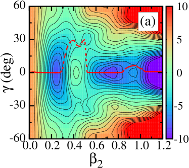
Figure 1: The projections of calculated total energy on the ($\beta_{2}$, $\gamma$) plane of quadrupole axial and triaxial ($\gamma$) deformations for ${}^{256}_{106}$Sg₁₅₀. At each deformation grid, a minimization has been performed over the hexadecapole deformation degrees of freedom $\alpha_{40}$, $\alpha_{42}$, $\alpha_{44}$ and $\beta_{4}$ in the subplots (a), (b), (c) and (d), respectively. The energy interval between neighbouring contour lines is 1 MeV. The red dash line denotes the possible fission pathway. See the text for more details.

The calculations of nuclear potential energy and/or Routhian surfaces are very helpful for understanding the structure properties (including the fission path) in nuclei. It is well known that theoretical description of fission is usually based on the analysis of the topography of the energy maps. The evolution of the potential energy surface as a function of the collective coordinates is of importance. We performed the nuclear potential-energy calculations using the deformed Woos-Saxon mean-field Hamiltonian in the deformation spaces ($\beta_{2}$, $\gamma$, $\alpha_{4\mu=0,2,4}$) and ($\beta_{2}$, $\gamma$, $\beta_{4}$). More elaborated investigation will include the parameters related to reflection asymmetric shapes because they are required for the description of the asymmetry in fission-fragment mass-distribution Zdeb2021 . In Fig. 1, the results of potential energy surfaces projected on ($\beta_{2}$, $\gamma$) plane and respectively minimized over the hexadecapole deformation $\alpha_{40}$, $\alpha_{42}$, $\alpha_{44}$ and $\beta_{4}$ are illustrated for ${}^{256}_{106}$Sg₁₅₀. In these maps, the $\beta_{2}$ and $\gamma$ deformation variables are directly presented as the horizontal and vertical coordinates in a Cartesian coordinate system, instead of the usual Cartesian quadrupole coordinates [$X=\beta_{2}\text{sin}(\gamma+30^{\circ})$, $Y=\beta_{2}\text{cos}(\gamma+30^{\circ})$] and the ($\beta_{2}$, $\gamma$) plane in the polar coordinate system. For the static energy surfaces, for guiding eyes, the $\gamma$ domain [$-60^{\circ}$, $60^{\circ}$] is adopted though, in principle, half is enough. One can see that two minima (at $\beta_{2}\approx 0.24$ and 0.7) appear and the double-humped barrier is reproduced but the second peak is lower than those in the actinide region Bjrnholm1980 . Calculated energy map shows that the hexadecapole deformation has no influence on the first minimum but can decrease the second minimum. It is found that the $\gamma$ destroy will strongly change the fission path, especially, between two minima.

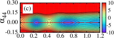
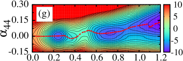
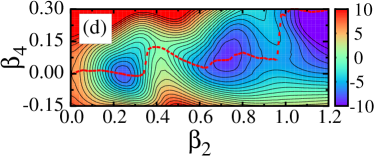
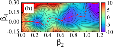
Figure 2: Similar to Fig. 1 but projections on ($\beta_{2}$,$\alpha_{40}$), ($\beta_{2}$,$\alpha_{42}$),($\beta_{2}$,$\alpha_{44}$) and ($\beta_{2}$,$\beta_{4}$) planes for ${}^{256}_{106}$Sg₁₅₀. Note that in the right four subfigures (e),(f),(g) and (h), the minimization was performed over the triaxial deformation $\gamma$ at each mesh grid. In (a),(b),(c) and (d) subplots, the triaxial destroy was not considered. See text for more information.

In order to understand how dependent calculated total energies are on these hexadecapole deformations $\alpha_{4\mu=0,2,4}$ (we focus here on the even-$\mu$ components), Figure 2 illustrates the corresponding 2D maps projected on ($\beta_{2}$, $\alpha_{4\mu=0,2,4}$) and ($\beta_{2}$, $\beta_{4}$) planes for ${}^{256}_{106}$Sg₁₅₀. To separately investigate the effects of different hexadecapole deformation parameters on the energy surfaces, in the left four subfigures of Fig. 2, we performed the calculations in 2D deformation spaces displayed by the horizontal and vertical coordinates, ignoring other degrees of freedom. It needs to be stressed that the hexadecapole deformation $\beta_{4}$ involves the fixed relationships of {$\alpha_{4\mu=0,2,4}$} and $\gamma$, cf. Eq. 7. For instance, three deformation parameters {$\alpha_{4\mu=0,2,4}$} can be determined in terms of a pair of given $\beta_{4}$ and $\gamma$ values. It can be seen from the left panel of Fig. 2 that only $\alpha_{40}$ (equivalently $\beta_{4}$ at $\gamma=0^{\circ}$) deformation changes the fission pathway. It seems that the non-axial deformation parameters $\alpha_{42}$ and $\alpha_{44}$ have no influence on the fission trajectory at this moment. In the right part, at each deformation point of the corresponding map, the minimization was performed over triaxial deformation $\gamma$. Indeed, one can find that non-zero {$\alpha_{4\mu=0,2,4}$} values appear along the fission pathway, indicating the three {$\alpha_{4\mu=0,2,4}$} deformations play a role during the calculations; see, e.g., Fig. 2(e)-(g). For simplicity of calculation and simultaneously including the effects of such three hexadecapole deformation parameters, total energy projection on the ($\beta_{2}$, $\beta_{4}$) plane is illustrated in Fig. 2(h), minimized over $\gamma$. It was often suggested that the 3-dimensional space ($\beta_{2},\gamma,\beta_{4}$) is the most important, e.g., cf. Ref. Sobiczewski2010 . Similar to the $\gamma$ deformation, the $\beta_{4}$ deformation has an obvious influence on the fission pathway after the first minimum for this nucleus. Moreover, the $\beta_{4}$ deformation always keeps a non-zero value after the first minimum.

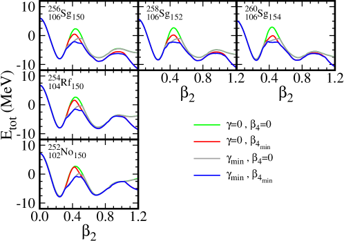
Figure 3: Four types of deformation energy curves as the function of quadrupole axial deformation $\beta_{2}$ for ${}^{256}_{106}$Sg₁₅₀ and its two isotopic and isotonic neighbours, namely, ${}^{258}_{106}$Sg₁₅₂, ${}^{260}_{106}$Sg₁₅₄, ${}^{254}_{104}$Rf₁₅₀ and ${}^{252}_{102}$No₁₅₀. At each $\beta_{2}$ point, the minimization was performed over $\gamma$ and/or $\beta_{4}$. The legends denote that whether or not total energy at each $\beta_{2}$ was minimized and, if so, with respect to what deformation parameter(s). See text for further explanations.

From the 2D energy $\beta_{2}$ vs $\gamma$ and $\beta_{2}$ vs $\beta_{4}$ maps, we can obtain the further energy projection e.g., on the $\beta_{2}$ direction. By such an operation, the total energy curve will be given, which is usually useful for extracting the information of fission barrier. Figure 3 illustrates four types of total energy curves in functions of $\beta_{2}$ for five selected nuclei ^256,258,260Sg, ²⁵⁴Rf and ²⁵²No. Note that the blue, grey, red and green lines respectively correspond to those curves whose energies are minimized over $\gamma$ and $\beta_{4}$; $\gamma$; $\beta_{4}$; and none. By them, one can see the evolution of the energy curves from both isotopic and isotonic directions. It seems that from the isotonic direction, ${}^{256}_{106}$Sg₁₅₀ is the critical nucleus in which the hexadecapole deformation $\beta_{4}$ always play a role after the first minimum. From this figure, we can obtain the equilibrium deformations of different minima and maxima, further the height of fission barriers. The impact of the triaxial and hexadecapole deformations on the energy curves can clearly evaluated. The inclusion of different deformation parameters can affect not only the height but also the shape of the fission barrier. As noted in Ref. Zdeb2021 , the tunneling probability through the fission barrier will depend exponentially on the square root of its height times its width, when approximated by a square potential barrier. One can find that the triaxial deformation can decrease the barrier hight, especially for the inner barrier e.g. in ²⁵⁶Sg. Nevertheless, the hexadecapole deformation (responsible for necking Tsekhanovich2019 ) decreases both the height and the width of the fission barrier. Even, as seen in ^256,258Sg, the least-energy fission path is strongly modified by the hexadecapole deformation after their first minima. After the second saddles, the effect of the hexadecapole deformation becomes significant in all selected nuclei. However, it was found that the octupole deformation will play an important role at the second saddle and after that, leading to a change of the obtained mass asymmetry at the scission point Wang2012 ; Zdeb2021 ; Lu2014 .

Table 2: The results of potential-energy-surface (PES) calculations for ground-state equilibrium deformation parameter $\beta_{2}$ and inner fission barriers $B_{f}$ for the 5 selected even-even nuclei, together with some other theoretical calculations for comparison; see the text for more descriptions.

Nuclei	$\beta_{2}$					$B_{f}$/MeV
	PES	HN Sobiczewski2001	FF Moller2016	HFBCS Goriely2001	ETFSI Aboussir1995	PES	HN Kowal2010	FFL Moller2009	ETFSI Mamdouh2001
${}^{260}_{106}$Sg154	0.243	0.247	0.242	0.31	0.25	6.49	6.28	5.84	4.6
${}^{258}_{106}$Sg152	0.242	0.247	0.252	0.27	0.25	6.16	6.22	5.93	4.7
${}^{256}_{106}$Sg150	0.243	0.246	0.252	0.25	0.27	5.88	5.46	5.30	—
${}^{254}_{104}$Rf150	0.243	0.247	0.252	0.27	0.27	6.44	5.74	5.87	5.3
${}^{252}_{102}$No150	0.243	0.249	0.250	0.30	0.26	7.01	6.52	6.50	5.8

In Table 2, the present results (calculated quadrupole deformation $\beta_{2}$ and fission barrier $B_{f}$) for five selected nuclei are confronted with other accepted theories (the experimental data are scarce so far), including the results of the heavy-nuclei (HN) model Sobiczewski2001 ; Kowal2010 , the fold-Yukawa (FY) single-particle potential and the finite-range droplet model (FRDM) Moller2016 , the Hartree-Fock-BCS (HFBCS) Goriely2001 , the fold-Yukawa (FY) single-particle potential and the finite-range liquid-drop model (FRLDM) Moller2009 , and the extended Thomas-Fermi plus Strutinsky integral (ETFSI) Aboussir1995 ; Mamdouh2001 methods. Comparison shows that these results are somewhat model-dependent but in good agreement with each other to a large extent. It can be found that the HFBCS calculation gave the larger equilibrium deformations and our calculation has the higher inner fission-barriers. Our calculated deformations may be underestimated to some extent, cf. Ref. Zhang2022 . As discussed by Dudek et al. Dudek1984 , the underestimated quadrupole deformation $\beta_{2}$ should be slightly modified by the empirical relationship $1.10\beta_{2}$-$0.03(\beta_{2})^{3}$. Within the framework of the same model, it can be seen that the selected five nuclei almost have the same $\beta_{2}$ in the PES, HN and FF (FY+FRDM) Moller2016 calculations. In the HFBCS and ETFSI calculations, the nucleus ²⁵⁶Sg has the largest and the smallest $\beta_{2}$ values in the five nuclei, respectively, but the differences are still rather small. Concerning the inner fission barriers, it seems that the present calculation may relatively overestimate the barriers. However, the present calculation has the same trends to the results given by HN and FFL (FY+FRLDM) Moller2009 calculations. For instance, the nucleus ²⁵⁶Sg has the smallest inner barrier in these five nuclei, in good agreement with those in HN and FFL calculations. In our previous publication Chai2018 , a lower $B_{f}$ about 4.8 MeV was obtained by using the universal parameter set. This value is lower about 1 MeV than the present calculation (5.88 MeV, as seen in the table) and lower than the values by HN and FFL calculations. The further experimental information is desirable. Interestingly, though the inner barrier of ²⁵⁶Sg is the lowest, its outer barrier ($\sim 2.72$ MeV) is higher than those in its isotopic neighbors ^258,260Sg ($\sim 2.52$ and 2.29 MeV). It is certainly expected that the outer barrier of ²⁵⁶Sg can relatively increase the survival probability of this superheavy nucleus, benifiting for the observation in experiment to some extent.

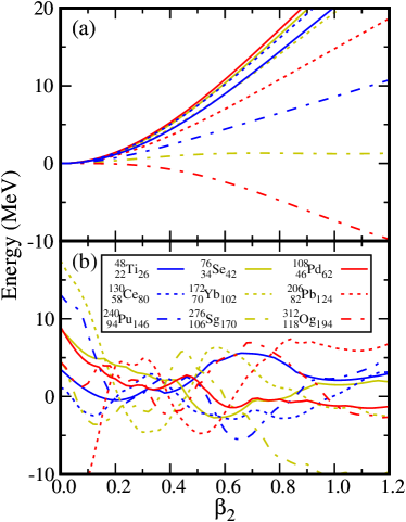
Figure 4: Macroscopic energies (a) and Shell correction energies (b) as the function of quadrupole axial deformation $\beta_{2}$ for several selected nuclei (see the legends, or cf. Ref. Meng2022 ) along the $\beta$-stability line. Note that during the calculation other deformation parameters are set to be zero.

In macroscopic-microscopic model, as is well known, the total energy is mainly determined by the liquid-drop energy and shell correction. In Fig. 4, to understand their evolution properties from light to heavy nuclei, we show the macroscopic energy and microscopic shell correction for arbitrarily selected nine nuclei along the $\beta$-stability line (cf. Ref. Meng2022 ). As excepted, one can see that with increasing mass number $A$ the macroscopic energy (the important contribution of fission barrier) is decreasing at a given $\beta_{2}$ (e.g., $\sim 0.4$, about the position of the first barrier;cf. Fig. 3) deformation, indeed, almost approaching zero in the superheavy region [e.g., with $Z\gtrsim 104$, see ${}^{276}_{106}$Sg₁₇₀ in Fig. 4(a), indicating the disappearance of the macroscopic fission barrier]. In particular, the calculated liquid-drop energy rapidly descends with increasing $\beta_{2}$ in the “heavier” superheavy nucleus ${}^{312}_{118}$Sg₁₉₄ which denotes that it is more difficult to bound such a heavy nucleon-system. Figure 3(b) illustrates the corresponding shell corrections for the selected nuclei mentioned above. Indeed, the energy staggering is rather large and combining the smoothed macroscopic energy, the potential pocket(s) can appear, which is the formation mechanism of superheavy nuclei.

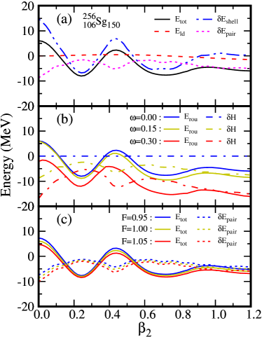
Figure 5: (a) Total energy $E_{tot}$ curve (together with its macroscopic liquid-drop energy $E_{ld}$ and microscopic shell correction and pairing correlation energies, namely, $\delta E_{shell}$ and $\delta E_{pair}$) vs $\beta_{2}$ deformation for the nucleus ${}^{256}_{106}$Sg₁₅₀. For simplicity, other deformation degrees of freedom were closed during the calculation. (b) Similar to (a) but for the total Routhian ($E_{rou}$) curves and the corresponding rotational contribution $\delta$H at three selected frequencies $\hbar\omega=0.00,0.15$ and 0.30 MeV. (c)Similar to (a) but for the total energy and the corresponding pairing correlation $\delta E$ at three selected pairing-strength factor $F=0.95,1.00$ and 1.05 (the adjusted pairing strength $G=FG_{0}$).

In Fig. 5, we provide the further evolution information on the total energy and its different components in functions of the quadrupole deformation $\beta_{2}$ for ${}^{256}_{106}$Sg₁₅₀. Figure 5(a) illustrates that total energy, together with the macroscopic liquid-drop energy $E_{ld}$, shell correction $\delta E_{shell}$ and pairing correlation $\delta E_{pair}$. For simplicity, other deformation degrees of freedom are ignored. In this nucleus, as seen, the macroscopic energy fully makes no contribution to the fission barrier. The barrier is mainly formed by the quantum shell effect. The inclusion of short-range pairing interaction always decreases the total energy, showing an irregular but relatively smoothed change (decreasing the barrier here). With increasing $\beta_{2}$, the shell effect tends to disapear. In the subfigure Fig. 5(b), we show the total Routhian and the rotational contribution at ground-state and two selected frquencies $\hbar\omega=$ 0.15 and 0.30 MeV, aiming to see the effect of the Coriolis force. One can see that, similar to the trend of the pairing correlation, the energy due to rotation will decrease the barrier because the energy difference e.g., at the positions of the first barrier and the first minimum is a negative value. It should be noted that the selected rotational frequencies respectively correspond to the values before and after the first band-crossing frequency in such a normal-deformed superheavy nucleus, e.g., cf. Ref. Wang2014 . Along the curve, the ground-state or yrast configuration for the nucleus may be rather different (see, e.g., Fig. 6, the occupied single-particle levels below the Fermi surface will generally be rather different). In Fig. 5(c), the total energy and its pairing correlation energy are illustrated with different pairing strengths by adjusting the factor $F$ (e.g., in $G=FG_{0}$, where $G_{0}$ is the orginal pairing strength). It can be noticed that the pairing correlation energy will decrease with increasing pairing strength $G$. Both at the barrier and the minimum, the effects seem to be very similar. At the large deformation region, the pairing correlation tends to a constant.

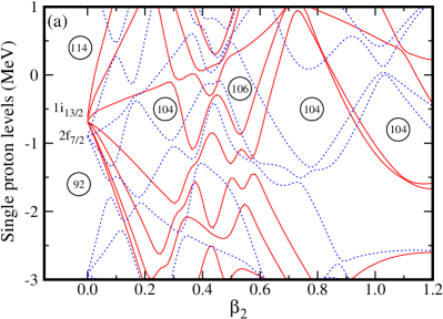
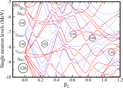
Figure 6: Calculated proton (a) and neutron (b) single-particle energies as functions of the quadrupole deformation $\beta_{2}$ for ${}^{256}_{106}$Sg₁₅₀, focusing on the domain near the Fermi surface. The levels with positive and negative parities are respectively denoted by red solid and blue dotted lines. Spherical single-particle orbitals (i.e., at $\beta_{2}$ = 0.0) in the window of interest are labeled by the quantum numbers $nlj$.

The microscopic structure of nuclei is primarily determined by the single-particle levels, especially near the Fermi level Baldo2020 . Experimentally, one can detect and investigate single-particle states by e.g., the inelastic electron scattering [like $(e,e^{\prime}p)$], the direct stripping and pick-up reactions [typically $(p,d)$ and $(d,p)$ reactions], $\beta$-decay rates, and so on Bertsch1983 ; Vaquero2020 . Because the measured single-particle states may be not pure, a rigorous definition of these states is given by the Green’s function formalism (cf. Ref. Baldo2020 ), showing that it is necessary to extract the spectroscopic factor. Such a quantity will provide an illustration of how much a single-particle level can be considered as a pure state and whether or not the correlations (e.g., the short- and long-range ones) beyond the mean field appear. Theoretically, the single-particle levels correspond to the eigenstates of the mean-field Hamiltonian (e.g., the Woods-Saxon-type one in this work). They are also the building blocks of the many-body wave functions, e.g., in self-consistent Hartree-Fock calculation. In Fig. 6, the single-particle levels near the proton and neutron Fermi surfaces are respectively illustrated in (a) and (b) parts. A set of conserved quantum numbers (associated with a complete set of commuting observables) are usually used for labeling the corresponding single-particle levels and wave functions. For instance, the spherical single-particle levels are denoted by the spherical quantum numbers $n,l$ and $j$ (corresponding the principal quantum number, the orbital angular momentum, and the total angular momentum, respectively). Similar to atomic spectroscopy, the notations $s$, $p$, $d$, $f$, $g$, $h$ $\cdots$ (corresponding to $l=$ $0$, $1$, $2$, $3$, $4$, $5$ $\cdots$, respectively) are used. Due to the strong spin-orbit coupling, the single particle state with $l$ will split into two states with $j$ = $l$ $\pm$ 1/2 (The degeneracy of each spherical single-particle level can be calculated by $2j+1$). In the present work, one can see that the expected shell structure and shell closure can be well reproduced. When deformed shape occurs, the $2j$+1 degeneracy will be broken and the spherical single-particle level will split into $j+1/2$ components (each one is typically double degenerate due to Kramers degeneracy). These deformed single-particle levels are generally described by asymptotic Nilsson quantum numbers $\Omega^{\pi}[Nn_{z}\Lambda]$, where $N$ is the total oscillator shell quantum number; $n_{z}$ stands the number of oscillator quanta in the $z$ direction (the direction of the symmetry axis); $\Lambda$ is the projection of angular momentum along the symmetry axis; $\Sigma$ is the projection of intrinsic spin along the symmetry axis; $\Omega$ is the projection of total angular momentum $j$ (including orbital $l$ and spin $s$) on the symmetry axis and $\Omega=\Lambda+\Sigma$. Note that the Nilsson labels are not given owing to space limitations. Similar to magnetic field, in the rotational coordinate system, the Coriolis force resulted from the non-inertial reference frame can also break the time reversal symmetry and mix the Nilsson states. Then, the single-particle Routhians can only be labeled by the conserved parity and signature $(\pi,\alpha)$ or $(\pi,r)$ (cf. Ref. Voigt1983 for the rigorous definition). It should be pointed out here that we did not perform the virtual crossing removal Bengtsson1985 of single-particle levels with same symmetries in these plots but this will not affect the identification of the single-particle levels. From Fig. 6, one can see that the shell gaps appear at the energy-minimum positions with lower level-densities and the higher level-densities occur at the saddle positions (cf. e.g., Fig. 5). The deformed neutron shells at $N=152$ and 162 are reproduced Oganessian2015 .

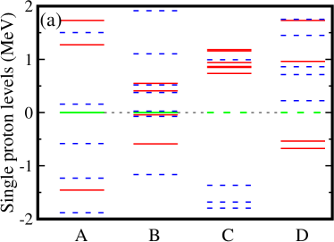
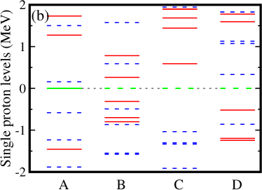
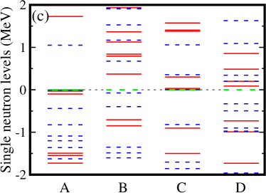
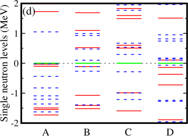
Figure 7: (a) Calculated proton single-particle levels for ${}^{256}_{106}$Sg₁₅₀ at the four typical $\beta_{2}$ deformation points ($A$, the 1st minimum; $B$, the 1st maximum;, $C$, the 2nd minimum; and $D$, the 2nd maximum) along the energy curve , see e.g., Fig. 3. In this plot, only $\beta_{2}$ deformation is considered for simplicity, corresponding to the blue energy curve in Fig. 3. (b) Similar to (a) but, in this plot, the energy is minimized over $\beta_{4}$ for each $\beta_{2}$ points, corresponding to the red energy curve in Fig. 3. (c) Similar to (a) but for neutron single-particle levels. (d) Similar to (b) but for neutron single-particle levels.

For a clear display about the level density near the minimum and saddle points, Figure 7 presents the proton and neutron single-particle levels at these corresponding deformation points. Note that the Fermi levels (the green levels) at the four typical points $A,B,C$ and $D$ are shifted to zero for comparison. The levels in Fig. 7(a) and (c) correspond to deformation conditions same to those in Figs. 5 and 6 where only the $\beta_{2}$ deformation is considered. In the right two subfigures of Fig. 7, at each $\beta_{2}$ point, the “realistic” $\beta_{4}$ value is taken into account (the equilibrium deformation is adopted after potential-energy minimization over $\beta_{4}$). Relative to the left two ones, the levels are rearranged to an extent by the hexadecapole deformation degree of freedom. As excepted, the level density is lower (higher) near the minimum (saddle) point, indicating the occurrence of a largely negative (positive) shell correction.

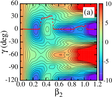
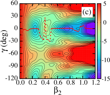
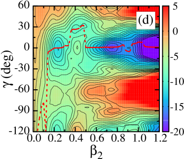
Figure 8: Similar to Fig. 1(d) but for total Routhian projections of ${}^{256}_{106}$Sg₁₅₀ at rotational frequencies $\hbar\omega=0.0$ (a), 0.1 (b), 0.2 (c) and 0.3 (d) MeV, respectively.

Figure 8 illustrates the total Routhian surfaces projected on the $\beta$ vs $\gamma$ plane for ${}^{256}_{106}$Sg₁₅₀ at several typical rotational frequencies. At each grid in the maps, the minimization of the total Routhian was performed over $\beta_{4}$. It needs to be stressed that the energy domains denoted by the color palettes are different in Figs. 8(c) and (d) for a better display. Under rotation, the triaxial deformation parameter $\gamma$ covers the range from $-120^{\circ}$ to $60^{\circ}$ because the three sectors ($-120^{\circ}$, $-60^{\circ}$), ($-60^{\circ}$, $0^{\circ}$) and ($0^{\circ}$, $60^{\circ}$) will represent rotation about the long, medium and short axes, respectively (the nucleus with triaxial shape). The nucleus with four $\gamma$ values $-120^{\circ}$, $-60^{\circ}$, $0^{\circ}$ and $60^{\circ}$ has the axially symmetric shape but different rotational orientation (cf. e.g., Ref. Wang2015 ). For instance, the triaxial deformation parameter $\gamma=-120^{\circ}$ during rotation denotes that a prolate nucleus with a non-collective rotation (namely, rotating around its symmetry axis; see, e.g., the low-frequency part on the fission path in Fig. 8(d)). The 1D cranking is limited in the present study. From this figure, one can see the evolution properties of the triaxiality and rotation axis for both the equilibrium shape and states along the fission path.

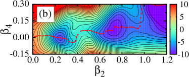
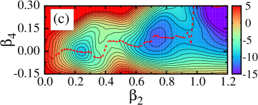
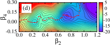
Figure 9: Similar to Fig. 2(h) but for total Routhian projections of ${}^{256}_{106}$Sg₁₅₀ at rotational frequencies $\hbar\omega=0.0$ (a), 0.1 (b), 0.2 (c) and 0.3 (d) MeV, respectively.

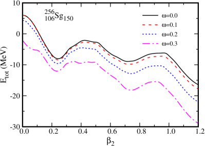
Figure 10: The calculated total Routhian curves against $\beta_{2}$ for ${}^{256}_{106}$Sg₁₅₀ at four selected frequencies $\hbar\omega=0.0$, 0.1, 0.2 and 0.3 MeV. At each $\beta_{2}$ point, the minimization was performed over $\gamma$ and $\beta_{4}$.

To investigate the hexadecapole-deformation effect under rotation, the total Routhian surfaces projected on the ($\beta_{2}$, $\beta_{4}$) plane are shown in Fig. 9 for ${}^{256}_{106}$Sg₁₅₀ at four selected rotational frequencies $\hbar\omega=0.0$, 0.1, 0.2 and 0.3 MeV, respectively. Note that the color palletes are slightly adjusted, similar to those in Fig. 8. It can be seen that the hexadecapole deformation $\beta_{4}$ can strongly decrease the total Routhian along the fission path, especially at high rotational frequency and large quadrupole deformation. In other words, the fission pathway will be modified by the the hexadecapole deformation $\beta_{4}$. It should be pointed out that from this figure one can find that part of the fission pathway evolutes along the border (with $\beta_{4}$=0.30) of the calculation domain, indicating the nucleus may possess a larger $\beta_{4}$ at this moment. Figure 10 illustrates the total Routhian curves in functions of $\beta_{2}$ for ${}^{256}_{106}$Sg₁₅₀ at the selected rotational frequencies mentioned above. The size and shape of the inner and outer barriers and their evolution with rotation can be evaluated conveniently. In the previous studies, e.g., in Refs. Wang2012 ; Lu2014 ; Kostryukov2021 , it was pointed out that the octupole correlation may further decrease the outer barrier in this mass region based on the PES calculation and fission fragment analysis. The outer barrier for this nucleus may finally be very low. It will be an open problem whether it will be able to play a certain role in blocking the fission process.

4. Conclusions

We evaluate the structure evolution along the fission pathway for ²⁵⁶Sg by using the multi-dimensional potential-energy(or Routhian)-surface calculations, focusing on the effects of triaxial and hexadecapole deformation and Coriolis force. Nuclear shape and microscopic single-particle structure are investigated and analyzed. The present results are compared with other theories. The properties of nuclear shape and fission barrier are analyzed by comparing with its neighboring even-even nuclei, showing a reasonable agreement. Based on the deformation energy or Routhian curves, the fission barriers are analyzed, focusing on their shapes, heights, and evolution with rotation. It is found that the triaxial deformation $\gamma$ decreases the potential energy on the landscape near the saddles but the hexadecapole deformation $\beta_{4}$ (especially the axial $\alpha_{40}$ component) modifies the least-energy fission path after the first minimum, especially in ²⁵⁶Sg. In addition, in contrast to the inner barrier, the outer barriers seem to have an increasing trend from ²⁶⁰Sg to ²⁵⁶Sg which may be benefit for blocking the fission of ²⁵⁶Sg to some extent. Next, it will be necessary to simultaneously consider the reflection asymmetry in a more reasonable deformation subspace.

Conflict of Interest

The authors declare that they have no known competing financial interests or personal relationships that could have appeared to influence the work reported in this paper.

References

References

- (1) M J A de Voigt, J Dudek and Z Szymański Rev. Mod. Phys. 55 949 (1983)
- (2) W P Liu, Z H Li, X X Bai, Y B Wang, B Guo, C H Peng, Y Yang, J Su, B Q Cui, S H Zhou, S Y Zhu, H H Xia, X L Guan, S Zeng, H Q Zhang, Y S Chen, H Q Tang, L Huang and B Y Feng Sci. China-Phys. Mech. Astron. 54 14 (2011)
- (3) E G Zhao and F Wang Chin. Sci. Bull. 56 3797 (2011)
- (4) Y T Oganessian and K P Rykaczewsk Phys. Today 68 32 (2015)
- (5) H Abusara, A V Afanasjev and P Ring Phys. Rev. C 82 044303 (2010)
- (6) P V Kostryukov, A Dobrowolski, B Nerlo-Pomorska, M Warda, Z Xiao, Y Chen, L Liu, J L Tian and K Pomorski Chin. Phys. C 45 124108 (2021)
- (7) B N Lu, J Zhao, E G Zhao and S G Zhou J. Phys.: Conf. Ser. 492 012014 (2014)
- (8) P Möller, A J Sierk, T Ichikawa, A Iwamoto, R Bengtsson, H Uhrenholt and S Åberg Phys. Rev. C 79 064304 (2009)
- (9) M Kowal, P Jachimowicz and A Sobiczewski Phys. Rev. C 82 014303 (2010)
- (10) P Möller, A J Sierk, T Ichikawa, A Iwamoto and M Mumpower Phys. Rev. C 91 024310 (2015)
- (11) A Gaamouci, I Dedes, J Dudek, A Baran, N Benhamouda, D Curien, H L Wang and J Yang Phys. Rev. C 103 054311 (2021)
- (12) G X Dong, X B Wang and S Y Yu Sci. China-Phys. Mech. Astron. 58 112004 (2015)
- (13) M Bender, K Rutz, P G Reinhard, J A Maruhn and W Greiner Phys. Rev. C 58 2126 (1998)
- (14) L Bonneau, P Quentin and D Samsœe Eur. Phys. J. A 21 391 (2004)
- (15) A Staszczak, A Baran, J Dobaczewski and W Nazarewicz Phys. Rev. C 80 014309 (2009)
- (16) A Staszczak, J Dobaczewski and W Nazarewicz Acta Phys. Pol. B 38 1589 (2007)
- (17) C Ling, C Zhou and Y Shi Eur. Phys. J. A 56 180 (2020)
- (18) Y J Chen, Y Su, G X Dong, L L Liu, Z G Ge and X B Wang Chin. Phys. C 46 024103 (2022)
- (19) A K Dutta, J M Pearson and F Tondeur Phys. Rev. C 61 054303 (2000)
- (20) A Mamdouh, J M Pearson, M Rayet and F Tondeur Nucl. Phys. A 679 337 (2001)
- (21) Z P Li, T Niks̆ić, D Vretenar, P Ring and J Meng Phys. Rev. C 81 064321 (2010)
- (22) P Ring, H Abusara, A V Afanasjev, G A Lalazissis, T Niks̆ić and D Vretenar Int. J. Mod. Phys. E 20 235 (2011)
- (23) W D Myers and W J Swiatecki Nucl. Phys. 81 1 (1966)
- (24) P Möller, W D Myers, W J Swiatecki and J Treiner At. Data Nucl. Data Tables 39 225 (1988)
- (25) K Pomorski and J Dudek Phys. Rev. C 67 044316 (2003)
- (26) Z Z Zhang, H L Wang, H Y Meng and M L Liu Nucl. Sci. Tech. 32 16 (2021)
- (27) I Dedes and J Dudek Phys. Rev. C 99 054310 (2019)
- (28) H Y Meng, H L Wang, Z Z Zhang and M L Liu Chin. Phys. C 46 104108 (2022)
- (29) H Y Meng, H L Wang and M L Liu Phys. Rev. C 105 014329 (2022)
- (30) J Yang, J Dudek, I Dedes, A Baran, D Curien, A Gaamouci, A Góźdź, A Pȩdrak, D Rouvel, H L Wang and J Burkat Phys. Rev. C 105 034348 (2022)
- (31) http://www.nndc.bnl.gov/
- (32) F P Heßberger, S Hofmann, V Ninov, P Armbruster, H Folger, G Münzenberg, H J Schött, A G Popeko, A V Yeremin, A N Andreyev and S Saro Z. Phys. A359 415 (1997)
- (33) H L Wang, H L Liu, F R Xu and C F Jiao Chin. Sci. Bull. 57 1761 (2012)
- (34) Q Z Chai, W J Zhao, M L Liu and H L Wang Chin. Phys. C 42 054101 (2018)
- (35) Q Z Chai, W J Zhao, H L Wang, M L Liu and F R Xu Prog. Theor. Exp. Phys. 2018 053D02 (2018)
- (36) Q Z Chai, W J Zhao and H L Wang Commun. Theor. Phys. 71 67 (2019)
- (37) Q Z Chai, W J Zhao and H L Wang Int. J. Mod. Phys. E 27 1850050 (2018)
- (38) H L Wang, Q Z Chai, J G Jiang and M L Liu Chin. Phys. C 38 074101 (2014)
- (39) A Sobiczewski, P Jachimowicz and M Kowal Int. J. Mod. Phys. E 19 493 (2010)
- (40) N Wang, L Dou, E G Zhao and S Werner Chin. Phys. Lett. 27 062502 (2010)
- (41) X J Bao, S Q Guo, H F Zhang and J Q Li J. Phys. G: Nucl. Part. Phys. 43 125105 (2016)
- (42) P Möller, J R Nix, W D Myers and W J Swiatecki At. Data Nucl. Data Tables 59 185 (1995)
- (43) T R Werner and J Dudek At. Data Nucl. Data Tables 50 179 (1992)
- (44) D R Inglis Phys. Rev. 96, 1059 (1954)
- (45) D R Inglis Phys. Rev. 97 701 (1955)
- (46) D R Inglis Phys. Rev. 103 1786 (1956)
- (47) W Nazarewicz, R Wyss and A Johnsson Nucl. Phys. A 503 285 (1989)
- (48) R Bengtsson, S E Larsson, G Leander, P Möller, S G Nilsson, S Åberg and Z Szymański Phys. Lett. B 57 301 (1975)
- (49) T R Werner, J Dudek At. Data Nucl. Data Tables 59 1 (1995)
- (50) K Neergård and V V Pashkevich Phys. Lett. B 59 218 (1975)
- (51) K Neergård, V V Pashkevich and S Frauendorf Nucl. Phys. A 262 61 (1976)
- (52) G Andersson, S E Larsson, G Leander, P Möller, S G Nilsson, I Ragnarsson, S Åberg, R Bengtsson, J Dudek, B Nerlo-Pomorska, K Pomorski and Z Szymański Nucl. Phys. A 268 205 (1976)
- (53) W Satuła, R Wyss and P Magierski Nucl. Phys. A 578 45 (1994)
- (54) J Dudek, B Herskind, W Nazarewicz, Z Szymanski and T R Werner Phys. Rev. C 38 940 (1988)
- (55) J Dudek, W Nazarewicz and T Werner Nucl. Phys. A 341 253 (1980)
- (56) A Bhagwat, X Vin̈as, M Centelles, P Schuk and R. Wyss Phys. Rev. C 81 044321 (2010)
- (57) A Bohr Mat. Fys. Medd. K. Dan. Vidensk. Selsk. 26 1 (1952)
- (58) H Y Meng, Y W Hao, H L Wang and M L Liu Prog. Theor. Exp. Phys. 2018 103D02 (2018)
- (59) S Ćwiok, J Dudek, W Nazarewicz, J Skalski and T Werner Comput. Phys. Commun. 46 379 (1987)
- (60) S G Nilsson, C F Tsang, A Sobiczewski, Z Szymański, C Gustafson, I L Lamm, P Möller and B Nilsson Nucl. Phys. A 131 1 (1969)
- (61) V M Strutinsky and F A Ivanyuk Nucl. Phys. A 255 405 (1975)
- (62) F A Ivanyuk and V M Strutinsky Z. Phys. A - Atomic Nuclei 286 291 (1978)
- (63) K Pomorski Phys. Rev. C 70 628 (2004)
- (64) M Bolsterli, E O Fiset, J R Nix and J L Norton Phys. Rev. C 5 1050 (1972)
- (65) T Vertse, A T Kruppa, R J Liotta, W Nazarewicz, N Sandulescu and T R Werner Phys. Rev. C 57 3089 (1998)
- (66) A T Kruppa, M Bender, W Nazarewicz, P G Reinhard, T Vertse and S Ćwiok Phys. Rev. C 61 034313 (2000)
- (67) H C Pradhan, Y Nogami and J Law Nucl. Phys. A 201 357 (1973)
- (68) P Möller and J R Nix Nucl. Phys. A 536 20 (1992)
- (69) F R Xu, W Satuła and R Wyss Nucl. Phys. A 669 119 (2000)
- (70) H Sakamoto and T Kishimoto Phys. Lett. B 245 321 (1990)
- (71) M Wakai and A Faessler Nucl. Phys. A 295 86 (1978)
- (72) M Diebel Nucl. Phys. A 419 221 (1984)
- (73) W Satuła and R Wyss Phys. Scr. T56 159 (1995)
- (74) P Ring, R Beck and H J Mang Z. Phys. 231 10 (1970)
- (75) A Zdeb, M Warda and L M Robledo Phys. Rev. C 104 014610 (2021)
- (76) S Bjørnholm and J E Lynn Rev. Mod. Phys. 52 725 (1980)
- (77) I Tsekhanovich, A N Andreyev, K Nishio, D Denis-Petit, K Hirose, H Makii, Z Matheson, K Morimoto, K Morita, W Nazarewicz, R Orlandi, J Sadhukhan, T Tanaka, M Vermeulen and M Warda Phys. Lett. B 790 583 (2019)
- (78) A Sobiczewski, I Muntian and Z Patyk, Phys. Rev. C 63 034306 (2001)
- (79) P Möller, A J Sierk, T Ichikawa and H Sagawa At. Data Nucl. Data Tables 109-110 1 (2016)
- (80) S Goriely, F Tondeur and J M Pearson At. Data Nucl. Data Tables 77 311 (2001)
- (81) Y Aboussir, J Pearson, A K Dutta and F Tondeur At. Data Nucl. Data Tables 61 127 (1995)
- (82) H H Zhang, H L Wang, H Y Meng, M L Liu and B Ding Phys. Scr. 97, 025303 (2022)
- (83) J Dudek, W Nazarewicz and A Faessler Nucl. Phys. A 412 61 (1984)
- (84) M Baldo Phys. At. Nucl. 83 161 (2020)
- (85) G F Bertsch, P F Bortignon and R A Broglia Rev. Mod. Phys. 55 287 (1983)
- (86) V Vaquero, A Jungclaus, T Aumann, J Tscheuschner, E V Litvinova, J A Tostevin, H Baba, D S Ahn, R Avigo, K Boretzky, A Bracco, C Caesar, F Camera, S Chen, V Derya, P Doornenbal, J Endres, N Fukuda, U Garg, A Giaz, M N Harakeh, M Heil, A Horvat, K Ieki, N Imai, N Inabe, N Kalantar-Nayestanaki, N Kobayashi, Y Kondo, S Koyama, T Kubo, I Martel, M Matsushita, B Million, T Motobayashi, T Nakamura, N Nakatsuka, M Nishimura, S Nishimura, S Ota, H Otsu, T Ozaki, M Petri, R Reifarth, J L Rodríguez-Sánchez, D Rossi, A T Saito, H Sakurai, D Savran, H Scheit, F Schindler, P Schrock, D Semmler, Y Shiga, M Shikata, Y Shimizu, H Simon, D Steppenbeck, H Suzuki, T Sumikama, D Symochko, I Syndikus, H Takeda, S Takeuchi, R Taniuchi, Y Togano, J Tsubota, H Wang, O Wieland, K Yoneda, J Zenihiro and A Zilges Phys. Rev. Lett. 124 022501 (2020)
- (87) T Bengtsson and I Ragnarsson Nucl. Phys. A 436 14 (1985)
- (88) H L Wang, J Yang, M L Liu and F R Xu Phys. Rev. C 92 024303 (2015)