A convergent entropy-dissipating BDF2 finite-volume
scheme for a population cross-diffusion system

Abstract.

A second-order backward differentiation formula (BDF2) finite-volume discretization for a nonlinear cross-diffusion system arising in population dynamics is studied. The numerical scheme preserves the Rao entropy structure and conserves the mass. The existence and uniqueness of discrete solutions and their large-time behavior as well as the convergence of the scheme are proved. The proofs are based on the G-stability of the BDF2 scheme, which provides an inequality for the quadratic Rao entropy and hence suitable a priori estimates. The novelty is the extension of this inequality to the system case. Some numerical experiments in one and two space dimensions underline the theoretical results.

1. Introduction

The design of structure-preserving finite-volume schemes for parabolic equations is fundamental to describe accurately the behavior of the numerical solutions to these equations. In the literature, usually implicit Euler time discretization are used to derive such schemes; see, e.g., [2, 3, 6, 9, 26]. However, implicit Euler schemes are only first order accurate in time, while finite-volume implementations often show second-order accuracy in space [9, 27] (also see [17] for an analytical result). In order to match the convergence rates in space and time, there is the need to design second-order time approximations, which lead to structure-preserving and convergent schemes. Some works suggest higher-order time discretizations (e.g. [8, 15, 19, 24, 29]), but they are only concerned with semidiscrete equations or different numerical methods, or they do not contain any numerical analysis. In this paper, we propose a second-order BDF two-point flux approximation finite-volume scheme, which conserves the mass and dissipates the Rao entropy, for a nonlinear cross-diffusion system arising in population dynamics. The quadratic structure of the Rao entropy allows us to extend the G-stability theory of Dahlquist to the system case, leading to existence, uniqueness, and convergence results.

The dynamics of the population density $u_{i}(x,t)$ of the $i$th species is modeled by the cross-diffusion equation

(1) $$\partial_{t}u_{i}=\operatorname{div}(\gamma\nabla u_{i}+u_{i}\nabla p_{i}(u)),\quad p_{i}(u):=\sum_{j=1}^{n}a_{ij}u_{j}\quad\mbox{in }\Omega,\ t>0,\ i=1,\ldots,n,$$

where $\Omega\subset{\mathbb{R}}^{d}$ ($d\geq 1$) is a bounded domain and $u=(u_{1},\ldots,u_{n})$. This model was derived rigorously from a moderately interacting stochastic particle system in a mean-field-type limit [11]. The parameter $\gamma>0$ is related to the stochastic diffusion of the particle system, and $a_{ij}\in{\mathbb{R}}$ describes the strength of the repulsive or attractive interaction between the $i$th and the $j$th species. We impose initial and no-flux boundary conditions,

(2) $$u_{i}(0)=u_{i}^{0}\quad\mbox{in }\Omega,\quad\nabla u_{i}\cdot\nu=0\quad\mbox{on }\partial\Omega,\ t>0,\ i=1,\ldots,n,$$

where $\nu$ is the exterior unit normal vector to $\partial\Omega$. In the absence of the diffusion parameter $\gamma$, (1) can be interpreted as a mass conservation equation with the partial velocity $\nabla p_{i}(u)$, which is determined according to Darcy’s law by the partial pressure $p_{i}(u)$. System (1) in one space dimension for two species, $\gamma=0$, and $\det(a_{ij})=0$ was first studied in [4], proving the global existence of segregated solutions (i.e., the supports of $u_{1}$ and $u_{2}$ do not intersect for all times if this holds true initially). This result was generalized to arbitrary space dimensions in [5], still for two species. For an arbitrary number of species, the existence of global weak solutions to (1)–(2) was shown in [25, Appendix B] if $\det(a_{ij})>0$ and the existence of local strong solutions was proved in [18] if $\det(a_{ij})=0$.

The matrix $A=(a_{ij})\in{\mathbb{R}}^{n\times n}$ does not need to be symmetric nor positive definite so that the diffusion matrix associated to (1) is generally neither symmetric nor positive definite too. A minimal requirement for local solvability at the linear level is the parabolicity in the sense of Petrovskii, which is satisfied if all eigenvalues of $A$ have a positive real part [1]. Global solvability is guaranteed under the detailed-balance condition, i.e., there exist $\pi_{1},\ldots,\pi_{n}>0$ such that $\pi_{i}a_{ij}=\pi_{j}a_{ji}$ for all $i\neq j$ [25, Theorem 17]. This condition also appears in the theory of time-continuous Markov chains generated by $A$, and $(\pi_{1},\ldots,\pi_{n})$ is the associated invariant measure. We assume this condition throughout this paper. It implies that $\widetilde{u}_{i}:=\pi_{i}u_{i}$ solves the system

$$\partial_{t}\widetilde{u}_{i}=\operatorname{div}\bigg{(}\widetilde{u}_{i}\sum_{j=1}^{n}\frac{a_{ij}}{\pi_{j}}\nabla\widetilde{u}_{j}\bigg{)},$$

with a symmetric positive definite matrix $(a_{ij}/\pi_{j})$. Consequently, we may assume, without loss of generality, that the matrix $A$ in (1) is already symmetric and positive definite.

Due to the nonlinear cross-diffusion structure, the analysis of (1) is highly nontrivial. The key idea of the analysis is to exploit the entropy structure of (1). This means that there exist Lyapunov functionals, called entropies, that are nonincreasing in time along solutions to (1)–(2) and that provide gradient estimates. In the present situation, these functionals are given by the Boltzmann (or Shannon) entropy $H_{B}$ and the Rao entropy $H_{R}$,

$$H_{B}(u)=\sum_{i=1}^{n}\int_{\Omega}u_{i}(\log u_{i}-1)\mathrm{d}x,\quad H_{R}(u)=\frac{1}{2}\int_{\Omega}u^{T}Au\mathrm{d}x,$$

giving formally the entropy equalities

(3) $$\frac{\mathrm{d}H_{B}}{\mathrm{d}t}+\int_{\Omega}\bigg{(}4\gamma\sum_{i=1}^{n}|\nabla\sqrt{u_{i}}|^{2}+\sum_{i,j=1}^{n}a_{ij}\nabla u_{i}\cdot\nabla u_{j}\bigg{)}\mathrm{d}x =0,$$

(4) $$\frac{\mathrm{d}H_{R}}{\mathrm{d}t}+\int_{\Omega}\bigg{(}\gamma\sum_{i,j=1}^{n}a_{ij}\nabla u_{i}\cdot\nabla u_{j}+\sum_{i=1}^{n}u_{i}|\nabla p_{i}(u)|^{2}\bigg{)}\mathrm{d}x =0,$$

and thus providing gradient bounds for $u_{i}$. The Boltzmann entropy is related to the thermodynamic entropy of the system, while the Rao entropy measures the functional diversity of the species [30].

Since the Boltzmann entropy $H_{R}$ is convex, the implicit Euler scheme preserves the entropy inequality (3) (see, e.g., [27] for a related system). The logarithmic structure of $H_{R}$ seems to prevent entropy stability in higher-order schemes like BDF or Crank–Nicolson approximations [22]. However, thanks to the quadratic structure of the Rao entropy $H_{R}$, we are able to prove stability of $H_{R}$ for the BFD2 approximation. To explain the idea, let ${\mathcal{T}}$ be a triangulation of $\Omega$ into control volumes $K\subset\Omega$ with measure $\operatorname{m}(K)$ and let $\Delta t$ be the time step size. Furthermore, let $u_{i,K}^{k}$ be an approximation of $u_{i}(x_{K},t_{k})$, where $x_{K}\in K$ and $t_{k}=k\Delta t$. We write the BDF2 discretization of (1) as

(5) $$\frac{\operatorname{m}(K)}{\Delta t}\bigg{(}\frac{3}{2}u_{i,K}^{k}-2u_{i,K}^{k}+\frac{1}{2}u_{i,K}^{k-2}\bigg{)}+\sum_{\sigma\in{\mathcal{E}}_{K}}{\mathcal{F}}_{i,K,\sigma}^{k}=0,$$

where ${\mathcal{E}}_{K}$ is the set of the edges (or faces) of $K$ and ${\mathcal{F}}_{i,K,\sigma}^{k}$ is the numerical flux, defined in (18) below. The usual idea to derive a priori bounds is to choose the test function $u_{i,K}^{k}$ in (5) and to use the inequality

(6) $$\bigg{(}\frac{3}{2}u_{i,K}^{k}-2u_{i,K}^{k}+\frac{1}{2}u_{i,K}^{k-2}\bigg{)}u_{i,K}^{k}\geq h_{0}(u_{i,K}^{k},u_{i,K}^{k-1})-h_{0}(u_{i,K}^{k-1},u_{i,K}^{k-2}),$$

where

$$h_{0}(a,b)=\frac{1}{4}\big{(}5a^{2}-4ab+b^{2}\big{)}=\frac{1}{4}\begin{pmatrix}a\\ b\end{pmatrix}^{T}\begin{pmatrix}5&-2\\ -2&1\end{pmatrix}\begin{pmatrix}a\\ b\end{pmatrix},\quad a,b\in{\mathbb{R}},$$

is a positive definite quadratic form. Assuming that ${\mathcal{F}}_{i,K,\sigma}^{k}u_{i,K}^{k}$ can be bounded from below, this gives a priori bounds for $(u_{i,K}^{k})^{2}$. Inequality (6) can be explained in the framework of Dahlquist’s G-stability theory [23].

In our case, we need the test function $p_{i}(u_{K}^{k})$ to derive the discrete analog of (4). Then the question is whether there exists a functional $h(u,v)$ such that

(7) $$\sum_{i=1}^{n}\bigg{(}\frac{3}{2}u_{i,K}^{k}-2u_{i,K}^{k}+\frac{1}{2}u_{i,K}^{k-2}\bigg{)}p_{i}(u_{K}^{k})\geq h(u_{K}^{k},u_{K}^{k-1})-h(u_{K}^{k-1},u_{K}^{k-2}).$$

Note that we need to sum over all species in this inequality. The main novelty of this paper is the observation that the scalar inequality (6) can be extended to inequality (7) for vectors $u$, $v\in{\mathbb{R}}^{n}$. Indeed, we show in Lemma 7 that (7) holds for

(8) $$h(u,v)=\frac{1}{4}(5u^{T}Au-4u^{T}Av+v^{T}Av)=\frac{1}{4}\begin{pmatrix}u\\ v\end{pmatrix}^{T}\begin{pmatrix}5A&-2A\\ -2A&A\end{pmatrix}\begin{pmatrix}u\\ v\end{pmatrix}$$

with $u,v\in{\mathbb{R}}^{n}$. Introducing the discrete Rao entropy by $H(u,v)=\sum_{K\in{\mathcal{T}}}\operatorname{m}(K)h(u,v)$ for piecewise constant functions $u$ and $v$, this yields the BDF2 analog of the Rao entropy inequality

$$H(u^{k},u^{k-1})+c\Delta t|u^{k}|_{1,2,{\mathcal{T}}}^{2}\leq H(u^{k-1},u^{k-2})\quad\mbox{for }k\geq 2,$$

where $|\cdot|_{1,2,{\mathcal{T}}}$ is the discrete $H^{1}(\Omega)$ norm, defined in Section 2.3, and $c>0$ depends on the smallest eigenvalue of $A$ and on $\gamma$. This inequality is the key for proving our main results:

• Existence and uniqueness of discrete solutions: There exists a solution $u_{i}^{k}$ to the BDF2 finite-volume scheme (5), which conserves the mass $\sum_{K\in{\mathcal{T}}}\operatorname{m}(K)u_{i,K}^{k}$ of the $i$th species and dissipates the discrete Rao entropy. Moreover, the solution is unique if $\Delta t/(\Delta x)^{d+2}$ is sufficiently small, where $\Delta x$ is the size of the mesh (Theorem 3). This unusual quotient comes from an inverse inequality needed to bound higher-order norms.

• Large-time behavior: The discrete solution $u_{i}^{k}$ converges for large times $k\to\infty$ to the constant steady state $\bar{u}_{i}=\operatorname{m}(\Omega)^{-1}\int_{\Omega}u_{i}^{0}\mathrm{d}x$ with a quasi-explicit exponential rate (Theorem 4). The proof uses the well-established relative entropy (or energy) method, but the two-step scheme requires an iteration of this argument.

• Convergence of the discrete scheme: The fully discrete solution converges to a solution to the semidiscrete problem if $\Delta x\to 0$, and the semidiscrete solution converges to a weak (nonnegative) solution to (1)–(2) as $\Delta t\to 0$ (up to subsequences; see Theorem 5).

• Convergence rate: If the solution to (1)–(2) is sufficiently smooth, the semidiscrete solution converges with order two, as expected for the BDF2 scheme (Theorem 6).

The paper is organized as follows. The numerical scheme and our main results are detailed in Section 2. In Section 3, we prove the existence and uniqueness of a discrete solution, while its large-time behavior is analyzed in Section 4. Section 5 is devoted to the convergence of the full scheme, and the second-order convergence in time is verified in Section 6. Finally, we present in Section 7 some numerical examples in one and two space dimensions.

2. Numerical scheme and main results

We need some simple auxiliary results and some notation before formulating the numerical scheme and the main results.

2.1. Some linear algebra

We denote by $|\cdot|$ the Euclidean norm on ${\mathbb{R}}^{n}$. Given a symmetric positive matrix $A\in{\mathbb{R}}^{n\times n}$, we introduce the weighted norm $|u|_{A}^{2}:=u^{T}Au$ and the weighted inner product $(u,v)_{A}:=u^{T}Av$ for $u,v\in{\mathbb{R}}^{n}$. With this notation, the discrete Rao entropy density can be written as

(9) $$h(u,v)=\frac{1}{4}(5|u|_{A}^{2}-4(u,v)_{A}+|v|_{A}^{2})\quad\mbox{for }u,v\in{\mathbb{R}}^{n}.$$

Denoting by $\lambda_{m}>0$ the smallest and by $\lambda_{M}>0$ the largest eigenvalue of $A$, it holds that

(10) $$\lambda_{m}|u|^{2}\leq|u|_{A}^{2}\leq\lambda_{M}|u|^{2}\quad\mbox{for }u\in{\mathbb{R}}^{n}.$$

Let $\lambda_{1},\ldots,\lambda_{n}>0$ be the eigenvalues of $A$. Then the eigenvalues of the matrix in (8) equal $(3\pm\sqrt{8})\lambda_{i}$ for $i=1,\ldots,n$. This shows that for $u,v\in{\mathbb{R}}^{n}$,

(11) $$\frac{1}{4}(3-\sqrt{8})(|u|_{A}^{2}+|v|_{A}^{2}) \leq h(u,v)\leq\frac{1}{4}(3+\sqrt{8})(|u|_{A}^{2}+|v|_{A}^{2}),$$

$$\frac{1}{4}(3-\sqrt{8})\lambda_{m}(|u|^{2}+|v|^{2}) \leq h(u,v)\leq\frac{1}{4}(3+\sqrt{8})\lambda_{M}(|u|^{2}+|v|^{2}).$$

2.2. Spatial domain and mesh

Let $d\geq 1$ and let $\Omega\subset{\mathbb{R}}^{d}$ be a bounded polygonal (if $d=2$) or polyhedral (if $d\geq 3$) domain. We associate to this domain an admissible mesh, given by (i) a family ${\mathcal{T}}$ of open polygonal or polyhedral control volumes, which are also called cells, (ii) a family ${\mathcal{E}}$ of edges (or faces if $d\geq 3$), and (iii) a family of points $(x_{K})_{K\in{\mathcal{T}}}$ associated to the control volumes and satisfying [21, Definition 9.1]. This definition implies that the straight line $\overline{x_{K}x_{L}}$ between two centers of neighboring cells is orthogonal to the edge (or face) $\sigma=K|L$ between two cells. For instance, triangular meshes with acute angles, Delaunay meshes, rectangular meshes, and Voronoï meshes satisfy this condition [21, Example 9.2]. The size of the mesh is given by $\Delta x=\max_{K\in{\mathcal{T}}}\operatorname{diam}(K)$. The family of edges ${\mathcal{E}}$ is assumed to consist of interior edges ${\mathcal{E}}_{\rm int}$ satisfying $\sigma\subset\Omega$ and boundary edges $\sigma\in{\mathcal{E}}_{\rm ext}$ satisfying $\sigma\subset\partial\Omega$. For a given $K\in{\mathcal{T}}$, ${\mathcal{E}}_{K}$ denotes the set of edges of $K$ with ${\mathcal{E}}_{K}={\mathcal{E}}_{{\rm int},K}\cup{\mathcal{E}}_{{\rm ext},K}$. For any $\sigma\in{\mathcal{E}}$, there exists at least one cell $K\in{\mathcal{T}}$ such that $\sigma\in{\mathcal{E}}_{K}$.

For given $\sigma\in{\mathcal{E}}$, we define the distance

$${\operatorname{d}}_{\sigma}=\begin{cases}{\operatorname{d}}(x_{K},x_{L})&\quad\mbox{if }\sigma=K|L\in{\mathcal{E}}_{{\rm int},K},\\ {\operatorname{d}}(x_{K},\sigma)&\quad\mbox{if }\sigma\in{\mathcal{E}}_{{\rm ext},K},\end{cases}$$

where d is the Euclidean distance in ${\mathbb{R}}^{d}$, and the transmissibility coefficient

(12) $$\tau_{\sigma}=\frac{\operatorname{m}(\sigma)}{{\operatorname{d}}_{\sigma}},$$

where $\operatorname{m}(\sigma)$ denotes the $(d-1)$-dimensional Lebesgue measure of $\sigma$. We suppose the following mesh regularity condition: There exists $0<\zeta\leq 1/2$ such that for all $K\in{\mathcal{T}}$ and $\sigma\in{\mathcal{E}}_{K}$,

(13) $${\operatorname{d}}(x_{K},\sigma)\geq\zeta{\operatorname{d}}_{\sigma}.$$

This is equivalent to

$$\eta\leq\frac{{\operatorname{d}}(x_{K},\sigma)}{{\operatorname{d}}(x_{L},\sigma)}\leq\frac{1}{\eta}\quad\mbox{for all }\sigma=K|L,$$

where $\eta=\zeta/(1-\zeta)\in(0,1]$. The statement follows by observing that ${\operatorname{d}}(x_{K},\sigma)+{\operatorname{d}}(x_{L},\sigma)={\operatorname{d}}(x_{K},x_{L})$ holds, which is a consequence of the orthogonality of $\sigma=K|L$ and $\overline{x_{K}x_{L}}$. Hence, the mesh regularity (13) means that the mesh is locally quasi-uniform. A consequence of the mesh regularity is the following estimate

(14) $$\sum_{\sigma\in{\mathcal{E}}_{{\rm int},K}}\operatorname{m}(\sigma){\operatorname{d}}_{\sigma}\leq\frac{1}{\zeta}\sum_{\sigma\in{\mathcal{E}}_{{\rm int},K}}\operatorname{m}(\sigma){\operatorname{d}}(x_{K},\sigma)=\frac{d}{\zeta}\operatorname{m}(K)\quad\mbox{for }K\in{\mathcal{T}},$$

where we used in the last step the formula for the volume of a (hyper-)pyramid.

2.3. Function spaces

Given a triangulation ${\mathcal{T}}$, let $T>0$, $N_{T}\in{\mathbb{N}}$ and introduce the time step size $\Delta t=T/N_{T}$ and the time steps $t_{k}=k\Delta t$ for $k=0,\ldots,N_{T}$. We set $\Omega_{T}=\Omega\times(0,T)$. The space of piecewise constant functions is defined by

$$V_{\mathcal{T}}=\bigg{\{}v:\Omega\to{\mathbb{R}}:\exists(v_{K})_{K\in{\mathcal{T}}}\subset{\mathbb{R}},\ v(x)=\sum_{K\in{\mathcal{T}}}v_{K}\mathbf{1}_{K}(x)\bigg{\}},$$

where $\mathbf{1}_{K}$ is the indicator function on $K$. To define a norm on this space, we define for $K\in{\mathcal{T}}$, $\sigma\in{\mathcal{E}}_{K}$,

$$v_{K,\sigma}=\begin{cases}v_{L}&\quad\mbox{if }\sigma=K|L\in{\mathcal{E}}_{{\rm int},K},\\ v_{K}&\quad\mbox{if }\sigma\in{\mathcal{E}}_{{\rm ext},K},\end{cases}\quad\textrm{D}_{K,\sigma}v:=v_{K,\sigma}-v_{K},\quad\textrm{D}_{\sigma}v:=|\mathrm{D}_{K,\sigma}v|.$$

Let $1\leq q<\infty$ and $v\in V_{\mathcal{T}}$. The discrete $W^{1,q}(\Omega)$ norm on $V_{\mathcal{T}}$ is given by

$$\|v\|_{1,q,{\mathcal{T}}}=\big{(}\|v\|_{0,q,{\mathcal{T}}}^{q}+|v|_{1,q,{\mathcal{T}}}^{q}\big{)}^{1/q},\quad\mbox{where}$$

$$\|v\|_{0,q,{\mathcal{T}}}^{q}=\sum_{K\in{\mathcal{T}}}\operatorname{m}(K)|v_{K}|^{q},\quad|v|_{1,q,{\mathcal{T}}}^{q}=\sum_{\sigma\in{\mathcal{E}}_{\rm int}}\operatorname{m}(\sigma){\operatorname{d}}_{\sigma}\bigg{|}\frac{\text{D}_{\sigma}v}{{\operatorname{d}}_{\sigma}}\bigg{|}^{q}\quad\mbox{for }v\in V_{\mathcal{T}}.$$

When $q=\infty$, we define $|v|_{1,\infty,{\mathcal{T}}}=\max_{\sigma\in{\mathcal{E}}_{\rm int}}|\mathrm{D}_{\sigma}v|/{\operatorname{d}}_{\sigma}$. If $v=(v_{1},\ldots,v_{n})\in V_{\mathcal{T}}^{n}$ is a vector-valued function, we write for notational convenience

$$\|v\|_{0,q,{\mathcal{T}}}=\sum_{i=1}^{n}\|v_{i}\|_{0,q,{\mathcal{T}}},\quad\|\nabla v\|_{0,q,{\mathcal{T}}}=\sum_{i=1}^{n}\|\nabla v_{i}\|_{0,q,{\mathcal{T}}}.$$

We associate to the discrete $W^{1,q}$ norm a dual norm with respect to the $L^{2}$ inner product:

$$\|v\|_{-1,q,{\mathcal{T}}}=\sup\bigg{\{}\int_{\Omega}vw\mathrm{d}x:w\in V_{\mathcal{T}},\ \|w\|_{1,q,{\mathcal{T}}}=1\bigg{\}}.$$

Finally, we introduce the space $V_{{\mathcal{T}},\Delta t}$ of piecewise constant functions with values in $V_{\mathcal{T}}$,

$$V_{{\mathcal{T}},\Delta t}=\bigg{\{}v:\Omega_{T}\to{\mathbb{R}}:\exists(v^{k})_{k=1,\ldots,N_{T}}\subset V_{\mathcal{T}},\ v(x,t)=\sum_{k=1}^{N_{T}}v^{k}(x)\mathbf{1}_{[t_{k-1},t_{k})}(t)\bigg{\}},$$

equipped with the $L^{2}(0,T;H^{1}(\Omega))$ norm

$$\|v\|_{L^{2}(0,T;H^{1}(\Omega))}=\left(\sum_{k=1}^{N_{T}}\Delta t\|v^{k}\|_{1,2,{\mathcal{T}}}^{2}\right)^{1/2}\quad\mbox{for all }v\in V_{{\mathcal{T}},\Delta t}.$$

2.4. Discrete gradient

The discrete gradient is defined on a dual mesh. For this, we define the cell $T_{K,\sigma}$ of the dual mesh for $K\in{\mathcal{T}}$ and $\sigma\in{\mathcal{E}}_{K}$:

• “Diamond”: Let $\sigma=K|L\in{\mathcal{E}}_{{\rm int},K}$. Then $T_{K,\sigma}$ is that cell whose vertices are given by $x_{K}$, $x_{L}$, and the end points of the edge $\sigma$. In higher dimensions, they might be (double) (hyper-)pyramids.

• “Triangle”: Let $\sigma\in{\mathcal{E}}_{{\rm ext},K}$. Then $T_{K,\sigma}$ is that cell whose vertices are given by $x_{K}$ and the end points of the edge $\sigma$.

The union of all “diamonds” and “triangles” $T_{K,\sigma}$ equals the domain $\Omega$ (up to a set of measure zero). The property that the straight line $\overline{x_{K}x_{L}}$ is orthogonal to the edge $\sigma=K|L$ implies that

$$\operatorname{m}(\sigma){\operatorname{d}}(x_{K},x_{L})=d\operatorname{m}(T_{K,\sigma})\quad\mbox{for all }\sigma=K|L\in{\mathcal{E}}_{\rm int}.$$

The approximate gradient of $v\in V_{{\mathcal{T}},\Delta t}$ is then defined by

$$\nabla^{{\mathcal{T}}}v(x,t)=\frac{\operatorname{m}(\sigma)}{\operatorname{m}(T_{K,\sigma})}\mathrm{D}_{K,\sigma}(v^{k})\nu_{K,\sigma}\quad\mbox{for }x\in T_{K,\sigma},\ t\in(t_{k-1},t_{k}],$$

where $\nu_{K,\sigma}$ is the unit vector that is normal to $\sigma$ and points outwards of $K$.

2.5. Numerical scheme

The initial functions are approximated by their $L^{2}(\Omega)$-orthogonal projection on $V_{\mathcal{T}}$:

(15) $$u_{i,K}^{0}=\frac{1}{\operatorname{m}(K)}\int_{K}u_{i}^{0}(x)\mathrm{d}x\quad\mbox{for all }K\in{\mathcal{T}},\ i=0,\ldots,n.$$

Let $u_{K}^{k-1}=(u_{1,K}^{k-1},\ldots,u_{n,K}^{k-1})$ for $K\in{\mathcal{T}}$ be given. Since the BDF2 scheme is a two-step method, we need a first time step which is computed from the implicit Euler method. The following time steps are determined from the BDF2 method. The finite-volume scheme reads as

(16) $$\frac{\operatorname{m}(K)}{\Delta t}(u_{i,K}^{1}-u_{i,K}^{0})+\sum_{\sigma\in{\mathcal{E}}_{K}}{\mathcal{F}}_{i,K,\sigma}^{1} =0,$$

(17) $$\frac{\operatorname{m}(K)}{\Delta t}\bigg{(}\frac{3}{2}u_{i,K}^{k}-2u_{i,K}^{k-1}+\frac{1}{2}u_{i,K}^{k-2}\bigg{)}+\sum_{\sigma\in{\mathcal{E}}_{K}}{\mathcal{F}}_{i,K,\sigma}^{k} =0,\quad k\geq 2,$$

for $i=1,\ldots,n$, $K\in{\mathcal{T}}$, and the numerical fluxes are given by

(18) $${\mathcal{F}}_{i,K,\sigma}^{k}=-\tau_{\sigma}\big{(}\gamma\textrm{D}_{K,\sigma}u_{i}^{k}+(u_{i,\sigma}^{k})^{+}\textrm{D}_{K,\sigma}p_{i}(u^{k})\big{)},$$

where $\tau_{\sigma}$ is defined in (12) and $z^{+}=\max\{0,z\}$ denotes the positive part of $z\in{\mathbb{R}}$. Finally, the so-called mobility is given by

(19) $$u_{i,\sigma}^{k}=M(u_{i,K}^{k},u_{i,L}^{k})\quad\mbox{for }\sigma=K|L,\quad u_{i,\sigma}^{k}=0\quad\mbox{else},$$

where $M$ is a general mean function satisfying

• $M:[0,\infty)^{2}\to[0,\infty)$ is Lipschitz continuous, satisfies $M(u,u)=u$ (consistency), and has linear growth in the sense $M(u,v)\leq|u|+|v|$ for $u,v\geq 0$.

• There exists $C>0$ such that $|M(u,v)-u|\leq C|u-v|$ for all $u,v\geq 0$.

Examples for $M$ are $M(u,v)=(u+v)/2$ or $M(u,v)=\max\{u,v\}$. Note that we do not need logarithmic mean functions like in [27], since we do not use the chain rule in the cross-diffusion part, so that we can use simpler expressions.

Remark 1 (Nonnegativity).

We truncate the mobility by $(u_{i,\sigma}^{k})^{+}$ in the numerical flux (18) to ensure the discrete Rao entropy inequality (see (21) below). Indeed, when testing (17) with $p_{i}(u^{k})$, we need that the sum $\sum_{\sigma\in{\mathcal{E}}_{\rm int}}\tau_{\sigma}(u_{i,\sigma}^{k})^{+}|\mathrm{D}_{K,\sigma}p_{i}(u^{k})|^{2}$ is nonnegative. Unfortunately, the quadratic Rao entropy does not allow us to prove the nonnegativity of the discrete solution, and standard maximum principle arguments do not apply here, so that the truncation cannot be removed. A positivity-preserving BDF2 finite-difference scheme was proposed in [13], but the proof relies on discrete $L^{\infty}(\Omega)$ bounds for $u^{k-1}$, which are not available in our case. Also the Shannon entropy does not help (as in [27]), since it is not compatible with the BDF2 discretization. Indeed, when we wish to derive a discrete analog of (3), we need a finite continuous functional $h(u,v)$ satisfying $h(u,u)=\sum_{i=1}^{n}u_{i}(\log u_{i}-1)$ (consistency condition) such that

$$\sum_{i=1}^{n}\bigg{(}\frac{3}{2}u_{i,K}^{k}-2u_{i,K}^{k-1}+\frac{1}{2}u_{i,K}^{k-2}\bigg{)}\log u_{i,K}^{k}\geq h(u_{K}^{k},u_{K}^{k-1})-h(u_{K}^{k-1},u_{K}^{k-2}).$$

If $u_{i,K}^{k}=u_{i,K}^{k-1}\to 0$ and $u_{i,K}^{k-2}>0$ for all $i\in\{1,\ldots,n\}$, the previous inequality converges to $-\infty\geq-h(0,u_{K}^{k-2})$, which is absurd. At least, we obtain nonnegative solutions in the limit $(\Delta x,\Delta t)\to 0$; see Theorem 5 below.

Remark 2 (Discrete integration by parts).

The fluxes $\mathcal{F}_{i,K,\sigma}^{k}$ are consistent approximations of the exact fluxes through the edges if we impose the conservation ${\mathcal{F}}_{i,K,\sigma}+{\mathcal{F}}_{i,L,\sigma}=0$ for all edges $\sigma=K|L$, requiring that they vanish on the Neumann boundary edges, i.e., ${\mathcal{F}}_{i,K,\sigma}=0$ for all $\sigma\in{\mathcal{E}}_{{\rm ext},K}$. In particular, for $v=(v_{K})\in V_{\mathcal{T}}$, the following discrete integration-by-parts formulas hold:

(20) $$\sum_{K\in{\mathcal{T}}}\sum_{\sigma\in{\mathcal{E}}_{K}}{\mathcal{F}}_{i,K,\sigma}v_{K}=-\sum_{\begin{subarray}{c}\sigma\in{\mathcal{E}}_{\rm int}\\ \sigma=K|L\end{subarray}}{\mathcal{F}}_{i,K,\sigma}\mathrm{D}_{K,\sigma}v,\quad\sum_{K\in{\mathcal{T}}}\sum_{\sigma\in{\mathcal{E}}_{K}}\tau_{\sigma}(\mathrm{D}_{K,\sigma}v)v_{K}=-|v|_{1,2,{\mathcal{T}}}^{2}.$$

2.6. Main results

We impose the following hypotheses.

• Data: $\Omega\subset{\mathbb{R}}^{d}$ with $d\geq 1$ is a bounded polygonal ($d=2$) or polyhedral ($d\geq 3$) domain, $T>0$, and $u^{0}\in L^{2}(\Omega;{\mathbb{R}}^{n})$. We set $\Omega_{T}=\Omega\times(0,T)$.

• Discretization: $\mathcal{T}$ is an admissible discretization of $\Omega$ satisfying (13) and $t_{k}=k\Delta t$ for $k=1,\ldots,N_{T}$.

• Coefficients: Let $\gamma>0$, and $A=(a_{ij})\in{\mathbb{R}}^{n\times n}$ is symmetric and positive definite. Let $\lambda_{m}>0$ and $\lambda_{M}>0$ be the smallest and largest eigenvalue of $A$, respectively.

The positivity of $\gamma$ is not needed for the existence analysis but for the convergence result, where we need higher-order integrability that is deduced via the discrete Gagliardo–Nirenberg inequality from the gradient bound. As mentioned in the introduction, the symmetry and positive definiteness of $A$ can be replaced by the positivity of the real parts of the eigenvalues of $A$ and the detailed-balance condition.

Recall the discrete BDF2 Rao entropy (see (9))

$$H(u,v)=\sum_{K\in{\mathcal{T}}}\operatorname{m}(K)h(u_{K},v_{K})=\frac{1}{4}\sum_{K\in{\mathcal{T}}}\operatorname{m}(K)\big{(}5|u_{K}|_{A}^{2}-4(u_{K},v_{K})_{A}+|v_{K}|_{A}^{2}\big{)}$$

for $u,v\in V_{\mathcal{T}}$. If $u=v$, this expression reduces to the usual discrete Rao entropy, used for the implicit Euler scheme, $H(u):=H(u,u)=\frac{1}{2}\sum_{K\in{\mathcal{T}}}\operatorname{m}(K)|u_{K}|_{A}^{2}$. Our first result is the existence of a discrete solution.

Theorem 3 (Existence and uniqueness of discrete solutions).

Let Hypotheses (H1)–(H3) hold, let $k\in{\mathbb{N}}$, and let $u^{k-1}\in V_{\mathcal{T}}^{n}$ be given. Then there exists a solution $u^{k}=(u_{1}^{k},\ldots,u_{n}^{k})\in V_{\mathcal{T}}^{n}$ to scheme (15)–(19) satisfying the discrete entropy inequality

(21) $$H(u^{k},u^{k-1})+\gamma\Delta t|A^{1/2}u^{k}|_{1,2,{\mathcal{T}}}^{2} \leq H(u^{k-1},u^{k-2})\quad\mbox{for }k\geq 2,$$

(22) $$H(u^{1})+\gamma\Delta t|A^{1/2}u^{1}|_{1,2,{\mathcal{T}}}^{2} \leq H(u^{0}),$$

and the scheme preserves the mass, $\sum_{K\in{\mathcal{T}}}\operatorname{m}(K)u_{i,K}^{k}=\int_{\Omega}u_{i}^{0}(x)\mathrm{d}x$ for $i=1,\ldots,n$, $k\geq 1$. These results also hold if $\gamma=0$. Furthermore, the solution is unique if $\gamma>0$, $\min_{\sigma\in{\mathcal{E}}_{\rm int}}{\operatorname{d}}_{\sigma}\geq\xi\Delta x$ for some $\xi>0$, and

$$\frac{\Delta t}{(\Delta x)^{d+2}}<\frac{C(d,\xi,\zeta)\gamma\lambda_{m}^{2}}{\lambda_{M}^{2}L^{2}H(u^{0})},$$

where $\zeta$ is defined in (13) and $L$ is the Lipschitz constant of the mean function $M$, defined in (19).

The existence of a discrete solution is proved by a fixed-point argument using the Brouwer degree theorem. Uniform estimates are obtained from the discrete Rao entropy inequality (21), where the BDF2 time approximation is estimated according to (7). This inequality, which is the key of our analysis, is proved in Lemma 7.

The uniqueness of solutions is proved by using the relative entropy method, which is equivalent to the energy method in the present case, since the Rao entropy is quadratic. In other words, we use the test function $p_{i}(u^{k})-p_{i}(v^{k})$ in the difference of the equations (17) satisfied by two discrete solutions $u^{k}$ and $v^{k}$. The cross-diffusion part contains cubic expressions, which turn into quadratic ones if $|A^{1/2}v^{k}|_{1,\infty,{\mathcal{T}}}$ is bounded (similar as in [12]). By an inverse inequality, this norm is bounded, up to some factor, by $(\Delta x)^{-d/2-1}\|A^{1/2}v^{k}\|_{0,2,{\mathcal{T}}}$, and $\|A^{1/2}v^{k}\|_{0,2,{\mathcal{T}}}$ is bounded because of (21)–(22). The remaining quadratic expression is estimated by using the gradient bounds (which requires $\gamma>0$) and the discrete $L^{2}(\Omega)$ bound coming from the time discretization (and introducing the factor $\Delta t$). The condition $\min_{\sigma\in{\mathcal{E}}_{\rm int}}{\operatorname{d}}_{\sigma}\leq\xi\Delta x$ is discussed in Remark 8.

For the next result, we set $\bar{u}_{i}=\operatorname{m}(\Omega)^{-1}\int_{\Omega}u_{i}^{0}\mathrm{d}x$ and recall the discrete Poincaré–Wirtinger inequality $\|v-\bar{v}\|_{0,2,{\mathcal{T}}}\leq C_{P}\zeta^{-1/2}|v|_{1,2,{\mathcal{T}}}$ for $v\in V_{\mathcal{T}}$ [7, Theorem 3.6]. Then, in view of (10),

(23) $$\|A^{1/2}(v-\bar{v})\|_{0,2,{\mathcal{T}}}\leq C_{P}\bigg{(}\frac{\lambda_{M}}{\lambda_{m}\zeta}\bigg{)}^{1/2}|A^{1/2}v|_{1,2,{\mathcal{T}}}\quad\mbox{for }v\in V_{\mathcal{T}}.$$

Theorem 4 (Large-time behavior).

Let $u^{k}$ be a solution to scheme (15)–(19). Then, for $k\geq 2$,

$$\|A^{1/2}(u^{k}-\bar{u})\|_{0,2,{\mathcal{T}}}\leq\sqrt{2}\|A^{1/2}(u^{0}-\bar{u})\|_{0,2,{\mathcal{T}}}(1+\kappa\Delta t)^{-(k-2)/4},$$

where $\kappa=4\gamma\lambda_{m}\zeta/((3+\sqrt{8})C_{P}^{2}\lambda_{M})$ and $C_{P}>0$ is the constant of the Poincaré–Wirtinger inequality (23).

The theorem states that $u^{k}$ converges exponentially fast to the constant steady state $\bar{u}$. Indeed, setting $\lambda_{\Delta t}:=\log(1+\kappa\Delta t)/(\Delta t)\nearrow\kappa$ as $\Delta t\to 0$, we have

$$\|A^{1/2}(u^{k}-\bar{u})\|_{0,2,{\mathcal{T}}}\leq\sqrt{2}\|A^{1/2}(u^{0}-\bar{u})\|_{0,2,{\mathcal{T}}}\exp(-\lambda_{\Delta t}t_{k}),\quad k\geq 2.$$

The proof of Theorem 4 is based on the discrete entropy inequality for the discrete relative Rao entropy $H(u^{k}-\bar{u},u^{k-1}-\bar{u})$, similar to (21). Indeed, by the discrete Poincaré–Wirtinger inequality, the discrete gradient term is bounded from below by the discrete $L^{2}(\Omega)$ norm of $u^{k}-\bar{u}$. As $H(u^{k}-\bar{u},u^{k-1}-\bar{u})$ can be estimated in terms of the discrete $L^{2}(\Omega)$ norms of $u^{k}-\bar{u}$ and $u^{k-1}-\bar{u}$, we need to iterate the entropy inequality a second time. Then, using (11), we arrive at the inequality

$$H(u^{k}-\bar{u},u^{k-1}-\bar{u})\leq(1+\kappa\Delta t)^{-1}H(u^{k-2}-\bar{u},u^{k-3}-\bar{u}),$$

and solving this recursion shows the result.

The numerial convergence of the scheme is proved in two steps. First, we show that the fully discrete solution $u_{m}^{k}\in V_{\mathcal{T}}^{n}$, indexed with the space grid size $\Delta x_{m}\to 0$ as $m\to\infty$, converges, up to a subsequence, to a solution $u^{k}\in H^{1}(\Omega)$ to the semidiscrete system

$$\frac{1}{\Delta t}(u_{i}^{1}-u_{i}^{0}) =\operatorname{div}(\gamma_{i}\nabla u_{i}^{1}+u_{i}^{1}\nabla p_{i}(u^{1})),$$

$$\frac{1}{\Delta t}\bigg{(}\frac{3}{2}u_{i}^{k}-2u_{i}^{k-1}+\frac{1}{2}u_{i}^{k-2}\bigg{)} =\operatorname{div}(\gamma_{i}\nabla u_{i}^{k}+(u_{i}^{k})^{+}\nabla p_{i}(u^{k}))\quad\mbox{in }\Omega,$$

with no-flux boundary conditions $\nabla u_{i}^{k}\cdot\nu=0$ on $\partial\Omega$, $i=1,\ldots,n$. Second, we prove that a subsequence of the sequence of semidiscrete solutions converges to a weak solution to (1)–(2) as $\Delta t\to 0$. Both steps may be summarized as follows (the precise convergence statements can be found in Propositions 9 and 11).

Theorem 5 (Convergence of the scheme).

Let Hypotheses (H1)–(H3) hold and let $({\mathcal{T}}_{m})_{m\in{\mathbb{N}}}$ be a sequence of admissible discretizations of $\Omega$ satisfying (13) uniformly in $m$ and $\Delta x_{m}\to 0$, $\Delta t_{m}\to 0$ as $m\to\infty$. Then the solution $(u_{m})$ to (15)–(19), constructed in Theorem 3, converges, up to a subsequence, as $m\to\infty$ to a function $u=(u_{1},\ldots,u_{n})$ satisfying $u_{i}\geq 0$ in $\Omega_{T}$ for $i=1,\ldots,n$, $u_{i}\in L^{2}(0,T;H^{1}(\Omega))$, $\partial_{t}u_{i}\in L^{2d+4}(0,T;W^{1,2d+4}(\Omega)^{\prime})$, and $u$ is a weak solution to (1)–(2).

The proof is based on suitable estimates uniform with respect to $\Delta x_{m}$ and $\Delta t_{m}$, derived from the entropy inequality (21). For the limit $\Delta x_{m}\to 0$, we follow the strategy of [10]. The compactness argument is different, since we still keep the time discretization. The limit $\Delta t_{m}\to 0$ is based on a higher-order integrability property derived from the Gagliardo–Nirenberg inequality and on the Aubin–Lions compactness lemma in the version of [16].

We need the condition $\gamma>0$ since the application of the discrete Gagliardo–Nirenberg inequality requires discrete gradient bounds. However, the term involving $p_{i}(u)$ only provides a bound for the discrete kinetic energy $\sum_{\sigma\in{\mathcal{E}}_{\rm int}}\tau_{\sigma}(u_{i,\sigma}^{k})^{+}|\mathrm{D}_{K,\sigma}p_{i}(u^{k})|^{2}$, from which we are unable to conclude gradient bounds. For the Euler scheme, this issue can be overcome by using the Boltzmann entropy inequality, which provides bounds in $L^{2}(0,T;H^{1}(\Omega))$ and $L^{\infty}(0,T;L^{1}(\Omega))$ (see (3)), and consequently in $L^{2+2/d}(\Omega_{T})$, which is the required higher-order integrability bound. As mentioned in the introduction, this entropy is not compatible with the BDF2 discretization. Therefore, the restriction $\gamma>0$ seems to be unavoidable with our approach.

Finally, we verify that the convergence of the semidiscrete system is of second order.

Theorem 6 (Second-order convergence).

Let $u^{k}$ be a solution to (31) and assume that the solution to (1)–(2) satisfies $u\in C^{3}([0,T];L^{2}(\Omega))\cap L^{\infty}(0,T;W^{1,\infty}(\Omega))$. Furthermore, let $\varepsilon>0$ be arbitrary and assume that

$$\Delta t<\frac{4(3-\sqrt{8})\gamma\lambda_{m}}{\lambda_{M}^{3}\|\nabla u\|_{L^{\infty}(\Omega_{T})}^{2}+4\gamma\lambda_{m}\varepsilon}.$$

Then there exists $C(\varepsilon)>0$, which is of order $\varepsilon^{-1/2}$ as $\varepsilon\to 0$ but independent of $\Delta t$, such that

$$\max_{k=1,\ldots,N_{T}}\|A^{1/2}(u_{i}^{k}-u_{i}(t_{k}))\|_{L^{2}(\Omega)}\leq C(\varepsilon)(\Delta t)^{2}\quad\mbox{for }i=1,\ldots,n.$$

We allow for the parameter $\varepsilon>0$ to minimize the time step size constraint; however, optimizing this constraint gives large constants $C(\varepsilon)$. The theorem is proved by analyzing the relative entropy $H(u(t_{k})-u^{k},u(t_{k-1})-u^{k-1})$, using a Taylor expansion for $u_{i}$ up to order $(\Delta t)^{3}$ (which requires a bound for $\partial_{t}^{3}u_{i}$), and iterating the entropy inequality once more. The resulting recursive inequality for the relative entropy can be solved, leading to the desired second-order bound.

3. Proof of Theorem 3

First, we make precise inequality (7). Recall definition (8) of $h(u,v)$ and let $H(u,v)=\sum_{K\in{\mathcal{T}}}\operatorname{m}(K)h(u,v)$ be the discrete Rao entropy.

Lemma 7 (BDF2 inequality).

It holds for $u,v,w\in{\mathbb{R}}^{n}$ that

$$\bigg{(}\frac{3}{2}u-2v+\frac{1}{2}w\bigg{)}^{T}Au=h(u,v)-h(v,w)+\frac{1}{4}|u-2v+w|_{A}^{2}.$$

In particular, for $u^{k}$, $u^{k-1}$, $u^{k-2}\in V_{\mathcal{T}}^{n}$,

$$\sum_{i,j=1}^{n}\sum_{K\in{\mathcal{T}}}\operatorname{m}(K)\bigg{(}\frac{3}{2}u_{i,K}^{k}-2u_{i,K}^{k-1}+\frac{1}{2}u_{i,K}^{k-2}\bigg{)}a_{ij}u_{j,K}^{k}\geq H(u^{k},u^{k-1})-H(u^{k-1},u^{k-2}).$$

Proof.

The proof follows by a direct computation. ∎

3.1. Definition and continuity of the fixed-point operator

We assume that $k\geq 2$, since the existence of a solution $u^{1}\in V_{\mathcal{T}}^{n}$ to the Euler scheme (17) satisfying (22) follows from [26, Theorem 1]. Let $u^{k-1}\in V_{\mathcal{T}}^{n}$ be given and let $R>0$, $\delta>0$. We set

$$Z_{R}=\big{\{}w=(w_{1},\ldots,w_{n})\in V_{\mathcal{T}}^{n}:\|w_{i}\|_{1,2,{\mathcal{T}}}<R\mbox{ for }i=1,\ldots,n\big{\}},$$

and let $w\in Z_{R}$. We consider the linear regularized problem

(24) $$\varepsilon\bigg{(}\sum_{\sigma\in{\mathcal{E}}_{K}}\tau_{\sigma}\mathrm{D}_{K,\sigma}w_{i}^{\varepsilon}-\operatorname{m}(K)w_{i,K}^{\varepsilon}\bigg{)}=\frac{\operatorname{m}(K)}{\Delta t}\bigg{(}\frac{3}{2}w_{i,K}-2u_{i,K}^{k-1}+\frac{1}{2}u_{i,K}^{k-2}\bigg{)}+\sum_{\sigma\in{\mathcal{E}}_{K}}{\mathcal{F}}^{+}_{i,K,\sigma}(w)$$

for $i=1,\ldots,n$, $K\in{\mathcal{T}}$, where

$${\mathcal{F}}^{+}_{i,K,\sigma}(w)=-\tau_{\sigma}\big{(}\gamma\mathrm{D}_{K,\sigma}w_{i}+w_{i,\sigma}^{+}\mathrm{D}_{K,\sigma}p_{i}(w)\big{)}.$$

The $\varepsilon$-regularization guarantees the coercivity of the associated bilinear form, while the truncation $w_{i,\sigma}^{+}$ is needed to obtain the nonnegativity of the entropy dissipation (see the estimate of $I_{6}$ below).

We claim that (24) has a unique solution $w^{\varepsilon}\in V_{\mathcal{T}}^{n}$. Indeed, since the mapping $g(w^{\varepsilon})=\varepsilon(\sum_{\sigma\in{\mathcal{E}}_{K}}\tau_{\sigma}\mathrm{D}_{K,\sigma}w_{i}^{\varepsilon}-\operatorname{m}(K)w_{i,K}^{\varepsilon})$ is linear and acting on finite-dimensional spaces, we only need to verify its injectivity. Let $w^{\varepsilon}$ be in the kernel of this mapping. Multiplying $g(w^{\varepsilon})=0$ by $w_{i,K}^{\varepsilon}$, summing over $K\in{\mathcal{T}}$, and using the discrete integration-by-parts formula (20) gives

$$0=\sum_{K\in{\mathcal{T}}}\sum_{\sigma\in{\mathcal{E}}_{K}}\tau_{\sigma}(\mathrm{D}_{K,\sigma}w_{i}^{\varepsilon})w_{i,K}^{\varepsilon}-\sum_{K\in{\mathcal{T}}}\operatorname{m}(K)(w_{i,K}^{\varepsilon})^{2}=-\|w_{i}^{\varepsilon}\|_{1,2,{\mathcal{T}}}^{2}.$$

This yields $w^{\varepsilon}=0$ and proves the claim.

Next, we show that the fixed-point mapping $F:Z_{R}\to V_{\mathcal{T}}^{n}$, $F(w)=w^{\varepsilon}$, is continuous. For this, we multiply (24) by $-w_{i,K}^{\varepsilon}$, sum over $K\in{\mathcal{T}}$, and use discrete integration by parts and the Cauchy–Schwarz inequality:

$$\varepsilon\|w_{i}^{\varepsilon}\|_{1,2,{\mathcal{T}}}^{2} =-\frac{1}{\Delta t}\sum_{K\in{\mathcal{T}}}\operatorname{m}(K)\bigg{(}\frac{3}{2}w_{i,K}-2u_{i,K}^{k-1}+\frac{1}{2}u_{i,K}^{k-2}\bigg{)}w_{i,K}^{\varepsilon}+\sum_{\begin{subarray}{c}\sigma\in{\mathcal{E}}_{\rm int}\\ \sigma=K|L\end{subarray}}{\mathcal{F}}_{i,K,\sigma}^{+}(w)\mathrm{D}_{K,\sigma}w_{i}^{\varepsilon}$$

(25) $$\leq\frac{1}{\Delta t}\bigg{\|}\frac{3}{2}w_{i}-2u_{i}^{k-1}+\frac{1}{2}u_{i}^{k-2}\bigg{\|}_{0,2,{\mathcal{T}}}\|w_{i}^{\varepsilon}\|_{0,2,{\mathcal{T}}}+\gamma|w_{i}|_{1,2,{\mathcal{T}}}|w_{i}^{\varepsilon}|_{1,2,{\mathcal{T}}}$$

$$\phantom{xx}{}-\sum_{\begin{subarray}{c}\sigma\in{\mathcal{E}}_{\rm int}\\ \sigma=K|L\end{subarray}}\tau_{\sigma}(w_{i,\sigma})^{+}\mathrm{D}_{K,\sigma}p_{i}(w)\mathrm{D}_{K,\sigma}w_{i}^{\varepsilon}.$$

For the last term, we use the Cauchy–Schwarz inequality and the fact that any norm on $V_{\mathcal{T}}^{n}$ is equivalent:

$$-\sum_{\begin{subarray}{c}\sigma\in{\mathcal{E}}_{\rm int}\\ \sigma=K|L\end{subarray}} \tau_{\sigma}(w_{i,\sigma})^{+}\mathrm{D}_{K,\sigma}p_{i}(w)\mathrm{D}_{K,\sigma}w_{i}^{\varepsilon}=-\sum_{j=1}^{n}\sum_{\begin{subarray}{c}\sigma\in{\mathcal{E}}_{\rm int}\\ \sigma=K|L\end{subarray}}\tau_{\sigma}a_{ij}w_{i,\sigma}^{+}\mathrm{D}_{K,\sigma}w_{i}\mathrm{D}_{K,\sigma}w_{i}^{\varepsilon}$$

$$\leq\sum_{j=1}^{n}\bigg{(}\sum_{\begin{subarray}{c}\sigma\in{\mathcal{E}}_{\rm int}\\ \sigma=K|L\end{subarray}}\tau_{\sigma}|\mathrm{D}_{\sigma}w_{i}^{\varepsilon}|^{2}\bigg{)}^{1/2}\bigg{(}\sum_{\begin{subarray}{c}\sigma\in{\mathcal{E}}_{\rm int}\\ \sigma=K|L\end{subarray}}\tau_{\sigma}a_{ij}^{2}(w_{i,\sigma}^{+})^{2}|\mathrm{D}_{\sigma}w_{j}|^{2}\bigg{)}^{1/2}$$

$$\leq C(A)\|w\|_{0,\infty,{\mathcal{T}}}\sum_{j=1}^{n}|w_{i}^{\varepsilon}|_{1,2,{\mathcal{T}}}|w_{j}|_{1,2,{\mathcal{T}}}\leq C(A,R)\|w_{i}^{\varepsilon}\|_{1,2,{\mathcal{T}}},$$

where we took into account the linear growth of $w_{i,\sigma}^{+}$ with respect to $w_{i,K}$ and $w_{i,L}$ (see (19)) and the definition of $Z_{R}$. Inserting these estimates into (25) and dividing by $\|w_{i}^{\varepsilon}\|_{1,2,{\mathcal{T}}}$, it follows that $\varepsilon\|w_{i}^{\varepsilon}\|_{1,2,{\mathcal{T}}}\leq C(A,R)$.

This bound allows us to verify the continuity of $F$. Indeed, let $w^{\ell}\to w$ as $\ell\to\infty$ and set $w^{\varepsilon,\ell}=F(w^{\ell})$. Then $(w^{\varepsilon,\ell})_{\ell\in{\mathbb{N}}}$ is uniformly bounded in the discrete $H^{1}(\Omega)$ norm. Therefore, there exists a subsequence, which is not relabeled, such that $w^{\varepsilon,\ell}\to w^{\varepsilon}$ as $\ell\to\infty$. Passing to the limit $\ell\to\infty$ in scheme (24), we see that $w^{\varepsilon}$ is a solution of the scheme and consequently $w^{\varepsilon}=F(w)$. Since the solution to the linear scheme (24) is unique, the entire sequence $(w^{\varepsilon,\ell})_{\ell\in{\mathbb{N}}}$ converges to $w^{\varepsilon}$, which shows the continuity of $F$.

3.2. Existence of a fixed point

According to the Brouwer degree fixed-point theorem, it is sufficient to show that for all $(w^{\varepsilon},\rho)\in\overline{Z}_{R}\times[0,1]$ such that $w^{\varepsilon}=\rho F(w^{\varepsilon})$, it holds that $w^{\varepsilon}\not\in\partial Z_{R}$ or, equivalently, $\|w^{\varepsilon}\|_{1,2,{\mathcal{T}}}<R$. We claim that this is true for sufficiently large $R>0$. Indeed, let $w^{\varepsilon}$ be such a fixed point. It satisfies

$$\varepsilon\bigg{(}\sum_{\sigma\in{\mathcal{E}}_{K}} \tau_{\sigma}\mathrm{D}_{K,\sigma}w_{i}^{\varepsilon}-\operatorname{m}(K)w_{i,K}^{\varepsilon}\bigg{)}$$

$$=\frac{\rho}{\Delta t}\operatorname{m}(K)\bigg{(}\frac{3}{2}w_{i,K}^{\varepsilon}-2u_{i,K}^{k-1}+\frac{1}{2}u_{i,K}^{k-2}\bigg{)}+\rho\sum_{\sigma\in{\mathcal{E}}_{K}}{\mathcal{F}}_{i,K,\sigma}^{+}(w^{\varepsilon}).$$

We multiply this equation by $-(\Delta t)p_{i}(w^{\varepsilon})$ and sum over $i=1,\ldots,n$, $K\in{\mathcal{T}}$. Then $0=I_{1}+I_{2}+I_{3}$, where

$$I_{1} =-\varepsilon\Delta t\sum_{i,j=1}^{n}\sum_{K\in{\mathcal{T}}}\bigg{(}\sum_{\sigma\in{\mathcal{E}}_{K}}\tau_{\sigma}\mathrm{D}_{K,\sigma}w_{i}^{\varepsilon}-\operatorname{m}(K)w_{i,K}^{\varepsilon}\bigg{)}a_{ij}w_{j,K}^{\varepsilon},$$

$$I_{2} =\rho\sum_{i,j=1}^{n}\sum_{K\in{\mathcal{T}}}a_{ij}\bigg{(}\frac{3}{2}w_{i,K}^{\varepsilon}-2u_{i,K}^{k-1}+\frac{1}{2}u_{i,K}^{k-2}\bigg{)}w_{j,K}^{\varepsilon},$$

$$I_{3} =-\rho\Delta t\sum_{i=1}^{n}\sum_{\begin{subarray}{c}\sigma\in{\mathcal{E}}_{\rm int}\\ \sigma=K|L\end{subarray}}{\mathcal{F}}_{i,K,\sigma}^{+}(w^{\varepsilon})\mathrm{D}_{K,\sigma}p_{i}(w^{\varepsilon}).$$

By discrete integration by parts,

$$I_{1} =\varepsilon\Delta t\sum_{i,j=1}^{n}\bigg{(}\sum_{\begin{subarray}{c}\sigma\in{\mathcal{E}}_{\rm int}\\ \sigma=K|L\end{subarray}}\tau_{\sigma}a_{ij}\mathrm{D}_{K,\sigma}w_{i}^{\varepsilon}\mathrm{D}_{K,\sigma}w_{j}^{\varepsilon}+\sum_{K\in{\mathcal{T}}}\operatorname{m}(K)a_{ij}w_{i,K}^{\varepsilon}w_{j,K}^{\varepsilon}\bigg{)}$$

$$\geq\varepsilon\lambda_{m}\Delta t(|w^{\varepsilon}|_{1,2,{\mathcal{T}}}^{2}+\|w^{\varepsilon}\|_{0,2,{\mathcal{T}}}^{2})=\varepsilon\lambda_{m}\Delta t\|w^{\varepsilon}\|_{1,2,{\mathcal{T}}}^{2},$$

and by Lemma 7,

$$I_{2}\geq H(w^{\varepsilon},u^{k-1})-H(u^{k-1},u^{k-2}).$$

For the third term, we obtain

$$I_{3} =\rho\Delta t\sum_{i,j=1}^{n}\sum_{\begin{subarray}{c}\sigma\in{\mathcal{E}}_{\rm int}\\ \sigma=K|L\end{subarray}}\tau_{\sigma}\gamma a_{ij}\mathrm{D}_{K,\sigma}w_{i}^{\varepsilon}\mathrm{D}_{K,\sigma}w_{j}^{\varepsilon}+\rho\Delta t\sum_{i=1}^{n}\sum_{\begin{subarray}{c}\sigma\in{\mathcal{E}}_{\rm int}\\ \sigma=K|L\end{subarray}}\tau_{\sigma}(w_{i,\sigma}^{\varepsilon})^{+}\bigg{(}\sum_{j=1}^{n}a_{ij}\mathrm{D}_{K,\sigma}w_{j}^{\varepsilon}\bigg{)}^{2}$$

$$\geq\gamma\rho\Delta t\sum_{\begin{subarray}{c}\sigma\in{\mathcal{E}}_{\rm int}\\ \sigma=K|L\end{subarray}}\tau_{\sigma}|A^{1/2}\mathrm{D}_{K,\sigma}w^{\varepsilon}|^{2}=\gamma\rho\Delta t|A^{1/2}w^{\varepsilon}|_{1,2,{\mathcal{T}}}^{2}.$$

Collecting these estimates gives

(26) $$\varepsilon\Delta t\|w^{\varepsilon}\|_{1,2,{\mathcal{T}}}^{2}+H(w^{\varepsilon},u^{k-1})+\gamma\Delta t\rho|A^{1/2}w^{\varepsilon}|_{1,2,{\mathcal{T}}}^{2}\leq H(u^{k-1},u^{k-2}).$$

Setting $R=(\varepsilon\Delta t)^{-1/2}H(u^{k-1},u^{k-2})^{1/2}+1$, we infer that $\|w^{\varepsilon}\|_{1,2,{\mathcal{T}}}^{2}\leq(R-1)^{2}<R^{2}$ and thus $w^{\varepsilon}\not\in\partial Z_{R}$, which shows the claim. Hence, there exists a fixed point $w^{\varepsilon}$ to $F$, which is a solution to

(27) $$\varepsilon\bigg{(}\sum_{\sigma\in{\mathcal{E}}_{K}}\tau_{\sigma}\mathrm{D}_{K,\sigma}w_{i}^{\varepsilon}-\operatorname{m}(K)w_{i,K}^{\varepsilon}\bigg{)}=\frac{\operatorname{m}(K)}{\Delta t}\bigg{(}\frac{3}{2}w_{i,K}^{\varepsilon}-2u_{i,K}+\frac{1}{2}u_{i,K}^{k-2}\bigg{)}+\sum_{\sigma\in{\mathcal{E}}_{K}}{\mathcal{F}}_{i,K,\sigma}(w^{\varepsilon}).$$

3.3. Limit $\varepsilon\to 0$

The solution $w^{\varepsilon}$ to (27) satisfies the regularized entropy inequality (26) with $\rho=1$, and the right-hand side is independent of $\varepsilon$ and $M$. It follows from the Bolzano–Weierstraß theorem that there exists a subsequence of $w^{\varepsilon}$, which is not relabeled, such that $w^{\varepsilon}\to w$ as $\varepsilon\to 0$. In particular, $\varepsilon^{1/2}w^{\varepsilon}\to 0$. Since the problem is finite dimensional, we can pass to the limit $\varepsilon\to 0$ in (27). Consequently, $u^{k}:=w$ is a solution to (17)–(19). The same limit in (26) with $\rho=1$ leads to the discrete entropy inequality of Theorem 3, which finishes the proof.

3.4. Uniqueness of solutions

Let $u^{k},v^{k}\in V_{\mathcal{T}}^{n}$ be two solutions to (15)–(19) with the same initial data $u^{0}=v^{0}$. We take the difference of the equations satisfied by $u^{k}$ and $v^{k}$, multiply the resulting equation by $p_{i}(u_{K}^{k})-p_{i}(v_{K}^{k})=\sum_{j=1}^{n}a_{ij}(u_{j,K}^{k}-v_{j,K}^{k})$, sum over $i=1,\ldots,n$, $K\in{\mathcal{T}}$, and use discrete integration by parts. This leads to $0=I_{4}+I_{5}+I_{6}$, where

$$I_{4} =\frac{3}{2\Delta t}\sum_{i,j=1}^{n}\sum_{K\in{\mathcal{T}}}\operatorname{m}(K)a_{ij}(u_{i,K}^{k}-v_{i,K}^{k})(u_{j,K}^{k}-v_{j,K}^{k})$$

$$I_{5} =\sum_{i,j=1}^{n}\sum_{\begin{subarray}{c}\sigma\in{\mathcal{E}}_{\rm int}\\ \sigma=K|L\end{subarray}}\tau_{\sigma}\gamma a_{ij}\mathrm{D}_{K,\sigma}(u_{i}^{k}-v_{i}^{k})\mathrm{D}_{K,\sigma}(u_{j}^{k}-v_{j}^{k})$$

$$I_{6} =\sum_{i,j,\ell=1}^{n}\sum_{\begin{subarray}{c}\sigma\in{\mathcal{E}}_{\rm int}\\ \sigma=K|L\end{subarray}}\tau_{\sigma}a_{ij}\big{(}(u_{i,\sigma}^{k})^{+}\mathrm{D}_{K,\sigma}u_{j}^{k}-(v_{i,\sigma}^{k})^{+}\mathrm{D}_{K,\sigma}v_{j}^{k}\big{)}a_{i\ell}\mathrm{D}_{K,\sigma}(u_{\ell}^{k}-v_{\ell}^{k}).$$

By the definition of the weighted norm, $I_{4}=(3/(2\Delta t))\|A^{1/2}(u^{k}-v^{k})\|_{0,2,{\mathcal{T}}}^{2}$. Furthermore,

$$I_{5}\geq\gamma\sum_{\begin{subarray}{c}\sigma\in{\mathcal{E}}_{\rm int}\\ \sigma=K|L\end{subarray}}\tau_{\sigma}|(A^{1/2}\mathrm{D}_{K,\sigma}(u^{k}-v^{k}))|^{2}=\gamma|A^{1/2}(u^{k}-v^{k})|_{1,2,{\mathcal{T}}}^{2}.$$

We add and subtract the term $(u_{i,\sigma}^{k})^{+}\mathrm{D}_{K,\sigma}v_{j}^{k}$ in $I_{6}$ and apply the Cauchy–Schwarz inequality:

$$I_{6} =\sum_{i,j,\ell=1}^{n}\sum_{\begin{subarray}{c}\sigma\in{\mathcal{E}}_{\rm int}\\ \sigma=K|L\end{subarray}}\tau_{\sigma}a_{ij}a_{i\ell}\Big{(}(u_{i,\sigma}^{k})^{+}\mathrm{D}_{K,\sigma}(u_{j}^{k}-v_{j}^{k})$$

$$\phantom{xx}{}+\big{(}(u_{i,\sigma}^{k})^{+}-(v_{i,\sigma}^{k})^{+}\big{)}\mathrm{D}_{K,\sigma}v_{j}^{k}\Big{)}\mathrm{D}_{K,\sigma}(u_{\ell}^{k}-v_{\ell}^{k})$$

$$=\sum_{i=1}^{n}\sum_{\begin{subarray}{c}\sigma\in{\mathcal{E}}_{\rm int}\\ \sigma=K|L\end{subarray}}\tau_{\sigma}(u_{i,\sigma}^{k})^{+}\bigg{(}\sum_{j=1}^{n}a_{ij}\mathrm{D}_{K,\sigma}(u_{j}^{k}-v_{j}^{k})\bigg{)}\bigg{(}\sum_{\ell=1}^{n}a_{i\ell}\mathrm{D}_{K,\sigma}(u_{\ell}^{k}-v_{\ell}^{k})\bigg{)}$$

$$\phantom{xx}{}-\sum_{\begin{subarray}{c}\sigma\in{\mathcal{E}}_{\rm int}\\ \sigma=K|L\end{subarray}}\tau_{\sigma}(A\mathrm{D}_{K,\sigma}v^{k})^{T}\big{[}\operatorname{diag}\big{(}(u_{i,\sigma}^{k})^{+}-(v_{i,\sigma}^{k})^{+}\big{)}A^{1/2}\big{]}(A^{1/2}\mathrm{D}_{K,\sigma}(u^{k}-v^{k}))$$

$$\geq-\bigg{(}\sum_{\begin{subarray}{c}\sigma\in{\mathcal{E}}_{\rm int}\\ \sigma=K|L\end{subarray}}\tau_{\sigma}|A\mathrm{D}_{K,\sigma}v^{k}|^{2}\big{|}\operatorname{diag}\big{(}(u_{i,\sigma}^{k})^{+}-(v_{i,\sigma}^{k})^{+}\big{)}A^{1/2}\big{|}^{2}\bigg{)}^{1/2}$$

$$\phantom{xx}{}\times\bigg{(}\sum_{\begin{subarray}{c}\sigma\in{\mathcal{E}}_{\rm int}\\ \sigma=K|L\end{subarray}}\tau_{\sigma}|A^{1/2}\mathrm{D}_{K,\sigma}(u^{k}-v^{k})|^{2}\bigg{)}^{1/2},$$

where $\operatorname{diag}((u_{i,\sigma}^{k})^{+}-(v_{i,\sigma}^{k})^{+})$ denotes the diagonal matrix with the entries $(u_{i,\sigma}^{k})^{+}-(v_{i,\sigma}^{k})^{+}$ for $i=1,\ldots,n$. Together with

$$|A\mathrm{D}_{K,\sigma}v^{k}|\leq|A^{1/2}||A^{1/2}\mathrm{D}_{K,\sigma}v^{k}|\leq\lambda_{M}^{1/2}|\mathrm{D}_{K,\sigma}v^{k}|_{A}\quad\mbox{and}$$

$$\big{|}\operatorname{diag}\big{(}(u_{i,\sigma}^{k})^{+}-(v_{i,\sigma}^{k})^{+}\big{)}A^{1/2}\big{|}\leq\big{|}\operatorname{diag}\big{(}(u_{i,\sigma}^{k})^{+}-(v_{i,\sigma}^{k})^{+}\big{)}\big{|}|A^{1/2}|$$

$$\phantom{xx}\leq\lambda_{M}^{1/2}\max_{i=1,\ldots,n}|(u_{i,\sigma}^{k})^{+}-(v_{i,\sigma}^{k})^{+}|\leq\lambda_{M}^{1/2}\max_{i=1,\ldots,n}|u_{i,\sigma}^{k}-v_{i,\sigma}^{k}|,$$

we find that

$$I_{6}\geq-\lambda_{M}|A^{1/2}v^{k}|_{1,\infty,{\mathcal{T}}}\max_{i=1,\ldots,n}\bigg{(}\sum_{\begin{subarray}{c}\sigma\in{\mathcal{E}}_{\rm int}\\ \sigma=K|L\end{subarray}}\operatorname{m}(\sigma){\operatorname{d}}_{\sigma}|u_{i,\sigma}^{k}-v_{i,\sigma}^{k}|^{2}\bigg{)}^{1/2}|A^{1/2}(u^{k}-v^{k})|_{1,2,{\mathcal{T}}}.$$

It remains to estimate the term involving the difference $|u_{i,\sigma}^{k}-v_{i,\sigma}^{k}|$. By the Lipschitz continuity of the mean function $M(u_{i,K}^{k},u_{i,L}^{k})=u_{i,\sigma}^{k}$ with Lipschitz constant $L>0$ and the mesh regularity (14),

$$\sum_{\begin{subarray}{c}\sigma\in{\mathcal{E}}_{\rm int}\\ \sigma=K|L\end{subarray}} \operatorname{m}(\sigma){\operatorname{d}}_{\sigma}|u_{i,\sigma}^{k}-v_{i,\sigma}^{k}|^{2}=\frac{1}{2}\sum_{K\in{\mathcal{T}}}\sum_{\sigma\in{\mathcal{E}}_{{\rm int},K}}\operatorname{m}(\sigma){\operatorname{d}}_{\sigma}|u_{i,\sigma}^{k}-v_{i,\sigma}^{k}|^{2}$$

$$\leq\frac{L^{2}}{2}\sum_{K\in{\mathcal{T}}}\sum_{\begin{subarray}{c}\sigma\in{\mathcal{E}}_{\rm int}\\ \sigma=K|L\end{subarray}}\operatorname{m}(\sigma){\operatorname{d}}_{\sigma}\big{(}|u_{i,K}^{k}-v_{i,K}^{k}|+|u_{i,L}^{k}-v_{i,L}^{k}|\big{)}^{2}$$

$$\leq 2L^{2}\sum_{K\in{\mathcal{T}}}\sum_{\begin{subarray}{c}\sigma\in{\mathcal{E}}_{\rm int}\\ \sigma=K|L\end{subarray}}\operatorname{m}(\sigma){\operatorname{d}}_{\sigma}|u_{i,K}^{k}-v_{i,K}^{k}|^{2}\leq\frac{2dL^{2}}{\zeta}\sum_{K\in{\mathcal{T}}}\operatorname{m}(K)|u_{i,K}^{k}-v_{i,K}^{k}|^{2}$$

$$=\frac{2dL^{2}}{\zeta}\|u^{k}-v^{k}\|_{0,2,{\mathcal{T}}}^{2}\leq\frac{2dL^{2}}{\lambda_{m}\zeta}\|A^{1/2}(u^{k}-v^{k})\|_{0,2,{\mathcal{T}}}^{2},$$

This shows that

$$I_{6}\geq-\frac{\lambda_{M}L}{\lambda_{m}^{1/2}}\bigg{(}\frac{2d}{\zeta}\bigg{)}^{1/2}|A^{1/2}v^{k}|_{1,\infty,{\mathcal{T}}}\|A^{1/2}(u^{k}-v^{k})\|_{0,2,{\mathcal{T}}}|A^{1/2}(u^{k}-v^{k})|_{1,2,{\mathcal{T}}}.$$

Collecting the estimates for $I_{4}$, $I_{5}$, and $I_{6}$ and using Young’s inequality gives

(28) $$\frac{3}{2\Delta t} \|A^{1/2}(u^{k}-v^{k})\|_{0,2,{\mathcal{T}}}^{2}+\gamma|A^{1/2}(u^{k}-v^{k})|_{1,2,{\mathcal{T}}}^{2}$$

$$\leq\frac{\lambda_{M}L}{\lambda_{m}^{1/2}}\bigg{(}\frac{2d}{\zeta}\bigg{)}^{1/2}|A^{1/2}v^{k}|_{1,\infty,{\mathcal{T}}}\|A^{1/2}(u^{k}-v^{k})\|_{0,2,{\mathcal{T}}}|A^{1/2}(u^{k}-v^{k})|_{1,2,{\mathcal{T}}}$$

$$\leq\frac{3}{2\Delta t}\|A^{1/2}(u^{k}-v^{k})\|_{0,2,{\mathcal{T}}}^{2}+\frac{\Delta t}{3}\frac{d\lambda_{M}^{2}L^{2}}{\lambda_{m}\zeta}|A^{1/2}v^{k}|_{1,\infty,{\mathcal{T}}}^{2}|A^{1/2}(u^{k}-v^{k})|_{1,2,{\mathcal{T}}}^{2}.$$

Now, the inverse inequality $|A^{1/2}v^{k}|_{1,\infty,{\mathcal{T}}}\leq C^{\prime}(d)(\Delta x)^{-d/2}\zeta^{-1/2}|A^{1/2}v^{k}|_{1,2,{\mathcal{T}}}$ [14, Prop. 3.10] and condition ${\operatorname{d}}_{\sigma}\geq\xi\Delta x$ imply that

$$|A^{1/2}v^{k}|_{1,\infty,{\mathcal{T}}}^{2} \leq\frac{C^{\prime}(d)^{2}}{(\Delta x)^{d}\zeta}\sum_{\begin{subarray}{c}\sigma\in{\mathcal{E}}_{\rm int}\\ \sigma=K|L\end{subarray}}\frac{\operatorname{m}(\sigma)}{{\operatorname{d}}_{\sigma}}|\mathrm{D}_{K,\sigma}(A^{1/2}v^{k})|^{2}$$

$$\leq\frac{C^{\prime}(d)^{2}}{(\Delta x)^{d}\zeta}\sum_{\begin{subarray}{c}\sigma\in{\mathcal{E}}_{\rm int}\\ \sigma=K|L\end{subarray}}\frac{\operatorname{m}(\sigma){\operatorname{d}}_{\sigma}}{\xi^{2}(\Delta x)^{2}}|\mathrm{D}_{K,\sigma}(A^{1/2}v^{k})|^{2}.$$

It follows from (14) and $|\mathrm{D}_{K,\sigma}(A^{1/2}v^{k})|^{2}\leq 2(|v_{K}^{k}|_{A}^{2}+|v_{L}^{k}|_{A}^{2})$ that

$$|A^{1/2}v^{k}|_{1,\infty,{\mathcal{T}}}^{2} \leq\frac{C^{\prime}(d)^{2}}{(\Delta x)^{d+2}\xi^{2}\zeta}\sum_{K\in{\mathcal{T}}}\frac{d}{\zeta}\operatorname{m}(K)|\mathrm{D}_{K,\sigma}(A^{1/2}v^{k})|^{2}$$

$$\leq\frac{2dC^{\prime}(d)^{2}}{(\Delta x)^{d+2}(\xi\zeta)^{2}}\sum_{K\in{\mathcal{T}}}\operatorname{m}(K)|A^{1/2}v^{k}_{K}|^{2}=\frac{C(d,\xi,\zeta)}{(\Delta x)^{d+2}}\|A^{1/2}v^{k}\|_{0,2,{\mathcal{T}}}^{2}.$$

Using this inequality as well as the bound

$$(3-\sqrt{8})\|A^{1/2}v^{k}\|_{0,2,{\mathcal{T}}}^{2}\leq 4H(v^{1},v^{0})\leq 2(3+\sqrt{8})(H(v^{1})+H(v^{0}))\leq 4(3+\sqrt{8})H(u^{0}),$$

obtained from (21)–(22), we deduce from (28), for another constant $C(d,\xi,\zeta)$ that

$$\gamma|A^{1/2}(u^{k}-v^{k})|_{1,2,{\mathcal{T}}}^{2}\leq C(d,\xi,\zeta)\frac{\lambda_{M}^{2}L^{2}}{\lambda_{m}}\frac{\Delta t}{(\Delta x)^{d+2}}H(u^{0})|A^{1/2}(u^{k}-v^{k})|_{1,2,{\mathcal{T}}}^{2}.$$

Then our smallness condition on $\Delta t/(\Delta x)^{d+2}$ implies that $|A^{1/2}(u^{k}-v^{k})|_{1,2,{\mathcal{T}}}=0$ and consequently, $u^{k}=v^{k}$, finishing the proof.

Remark 8.

The quasi-uniform condition $\min_{\sigma\in{\mathcal{E}}_{\rm int}}{\operatorname{d}}_{\sigma}\geq\xi\Delta x>0$ implies condition (23) in [20], since the mesh regularity (13) gives $\min_{K\in{\mathcal{T}}}\min_{\sigma\in{\mathcal{E}}_{K}}{\operatorname{d}}(x_{K},\sigma)/\operatorname{diam}(K)\geq\zeta{\operatorname{d}}_{\sigma}/\Delta x\geq\zeta\xi>0$. It also implies the mesh regularity condition $\operatorname{diam}(K)/{\operatorname{d}}(x_{K},\sigma)\leq\xi_{0}$ in [20, (9)], since, because of (13) again, $\operatorname{diam}(K)/{\operatorname{d}}(x_{K},\sigma)\leq\Delta x/(\zeta{\operatorname{d}}_{\sigma})\leq 1/(\xi\zeta)=:\xi_{0}$. It can be seen by considering quadratic cells that the quasi-uniform condition $\min_{\sigma\in{\mathcal{E}}_{\rm int}}{\operatorname{d}}_{\sigma}\geq\xi\Delta x>0$ generally does not imply the mesh regularity condition (13) and vice versa, so both conditions are independent from each other.

4. Proof of Theorem 4

We infer from mass conservation, $\sum_{K\in{\mathcal{T}}}\operatorname{m}(K)u_{i,K}^{k}=\sum_{K\in{\mathcal{T}}}\operatorname{m}(K)u_{i,K}^{0}=\operatorname{m}(\Omega)\bar{u}_{i}$, that

$$H(u^{k}-\bar{u},u^{k-1}-\bar{u}) =H(u^{k},u^{k-1})+\frac{1}{2}\sum_{K\in{\mathcal{T}}}\operatorname{m}(K)\big{(}|\bar{u}|_{A}^{2}-3(u_{K}^{k},\bar{u})_{A}+(u_{K}^{k-1},\bar{u})_{A}\big{)}$$

$$=H(u^{k},u^{k-1})-\frac{1}{2}\operatorname{m}(\Omega)|\bar{u}|_{A}^{2}.$$

Then the entropy inequality (21) shows that

(29) $$H(u^{k}-\bar{u},u^{k-1}-\bar{u})+\gamma\Delta t|A^{1/2}u^{k}|_{1,2,{\mathcal{T}}}^{2}\leq H(u^{k-1}-\bar{u},u^{k-2}-\bar{u})$$

for $k\geq 2$. Another iteration gives, for $k\geq 3$,

$$H(u^{k}-\bar{u},u^{k-1}-\bar{u})+\gamma\Delta t\big{(}|A^{1/2}u^{k}|_{1,2,{\mathcal{T}}}^{2}+|A^{1/2}u^{k-1}|_{1,2,{\mathcal{T}}}^{2}\big{)}\leq H(u^{k-2}-\bar{u},u^{k-3}-\bar{u}).$$

Hence, taking into account the discrete Poincaré–Wirtinger inequality (23),

$$H(u^{k}-\bar{u},u^{k-1}-\bar{u}) +\frac{\gamma\lambda_{m}\zeta}{C_{P}^{2}\lambda_{M}}\Delta t\big{(}\|A^{1/2}(u^{k}-\bar{u})\|_{0,2,{\mathcal{T}}}^{2}+\|A^{1/2}(u^{k-1}-\bar{u})\|_{0,2,{\mathcal{T}}}^{2}\big{)}$$

$$\leq H(u^{k-2}-\bar{u},u^{k-3}-\bar{u}),$$

and the norm equivalence (10),

$$H(u^{k}-\bar{u},u^{k-1}-\bar{u})+\frac{4\gamma\lambda_{m}\zeta\Delta t}{(3+\sqrt{8})C_{P}^{2}\lambda_{M}}H(u^{k}-\bar{u},u^{k-1}-\bar{u})\leq H(u^{k-2}-\bar{u},u^{k-3}-\bar{u}).$$

This can be written as

$$H(u^{k}-\bar{u},u^{k-1}-\bar{u})\leq(1+\kappa\Delta t)^{-1}H(u^{k-2}-\bar{u},u^{k-3}-\bar{u}),$$

where $\kappa=4\gamma\lambda_{m}\zeta/((3+\sqrt{8})C_{P}^{2}\lambda_{M})$. Depending on whether $k$ is odd or even, we resolve this iteration as follows:

$$H(u^{2\ell+1}-\bar{u},u^{2\ell}-\bar{u}) \leq(1+\kappa\Delta t)^{-\ell}H(u^{1}-\bar{u},u^{0}-\bar{u}),$$

$$H(u^{2\ell+2}-\bar{u},u^{2\ell+1}-\bar{u}) \leq(1+\kappa\Delta t)^{-\ell}H(u^{2}-\bar{u},u^{1}-\bar{u})$$

$$\leq(1+\kappa\Delta t)^{-\ell}H(u^{1}-\bar{u},u^{0}-\bar{u}),$$

where we used (29) in the last step. As in both cases $\ell\geq(k-2)/2$, we conclude that

(30) $$H(u^{k}-\bar{u},u^{k-1}-\bar{u})\leq(1+\kappa\Delta t)^{-(k-2)/2}H(u^{1}-\bar{u},u^{0}-\bar{u}).$$

We want to express this inequality in terms of the $\|A^{1/2}(\cdot)\|_{0,2,{\mathcal{T}}}$ norm. We observe that, by Young’s inequality, $\|A^{1/2}(u^{k}-\bar{u})\|_{0,2,{\mathcal{T}}}^{2}\leq 4H(u^{k}-\bar{u},u^{k-1}-\bar{u})$ and, in view of (22),

$$H(u^{1}-\bar{u},u^{0}-\bar{u}) =H(u^{1})-H(\bar{u})\leq H(u^{0})-H(\bar{u})$$

$$=H(u^{0}-\bar{u})=\frac{1}{2}\|A^{1/2}(u^{0}-\bar{u})\|_{0,2,{\mathcal{T}}}^{2}.$$

Then we deduce from (30) that

$$\|A^{1/2}(u^{k}-\bar{u})\|_{0,2,{\mathcal{T}}}^{2} \leq 4H(u^{k}-\bar{u},u^{k-1}-\bar{u})\leq 4(1+\kappa\Delta t)^{-(k-2)/2}H(u^{1}-\bar{u},u^{0}-\bar{u})$$

$$\leq 2(1+\kappa\Delta t)^{-(k-2)/2}\|A^{1/2}(u^{0}-\bar{u})\|_{0,2,{\mathcal{T}}}^{2},$$

which concludes the proof.

5. Proof of Theorem 5

We split the proof into two parts. We first prove the convergence in the space variable and then the convergence in the time variable. An alternative is to show the convergence in both variables simultaneously; see, e.g., [27].

5.1. Convergence in space

We show the following result for $\Delta x\to 0$.

Proposition 9 (Convergence in space).

Let the assumptions of Theorem 5 hold and let $(u_{m}^{k})$ be the sequence of solutions to (15)–(19) constructed in Theorem 3 associated to an admissible mesh ${\mathcal{T}}_{m}$ with mesh size $\Delta x_{m}$ for $m\in{\mathbb{N}}$ satisfying $\Delta x_{m}\to 0$ as $m\to\infty$. Then there exists a subsequence which is not relabeled such that $u_{i,m}^{k}\to u_{i}^{k}$ strongly in $L^{2}(\Omega)$ as $m\to\infty$ and $u_{i}^{k}$ solves for all $\phi_{i}\in W^{1,\max\{2,d\}}(\Omega)$, $i=1,\ldots,n$,

(31) $$\frac{1}{\Delta t}\int_{\Omega}\bigg{(}\frac{3}{2}u_{i}^{k}-2u_{i}^{k-1}+\frac{1}{2}u_{i}^{k-2}\bigg{)}\phi_{i}\mathrm{d}x+\int_{\Omega}\big{(}\gamma\nabla u_{i}^{k}+(u_{i}^{k})^{+}\nabla p_{i}(u^{k})\big{)}\cdot\nabla\phi_{i}\mathrm{d}x=0.$$

Proof.

For fixed $\Delta t$, the discrete entropy inequality in Theorem 3 provides a uniform bound for $\|u_{m}^{k}\|_{1,2,{\mathcal{T}}_{m}}$. Then, by the discrete Rellich–Kondrachov compactness theorem [21, Lemma 5.6], there exists a subsequence of $(u_{m}^{k})=(u_{1,m}^{k},\ldots,u_{n,m}^{k})$, which is not relabeled, such that $u_{m}^{k}\to u^{k}$ strongly in $L^{2}(\Omega)$ as $m\to\infty$. Moreover, the sequence of discrete gradients $(\nabla^{m}u_{m}^{k})$ converges weakly in $L^{2}(\Omega)$ to some function which can be identified by $\nabla u^{k}$; see [10, Lemma 4.4]. Let $\phi_{i}\in C^{2}(\overline{\Omega})$ and set $\phi_{i,K}:=\phi_{i}(x_{K})$ for $K\in{\mathcal{T}}$. Then the limit $\Delta x_{m}\to 0$ in the BDF2 approximation becomes

$$\frac{1}{\Delta t}\sum_{K\in{\mathcal{T}}}\operatorname{m}(K)\bigg{(}\frac{3}{2}u_{i,K}^{k}-2u_{i,K}^{k-1}+\frac{1}{2}u_{i,K}^{k-2}\bigg{)}\phi_{i,K}\to\frac{1}{\Delta t}\int_{\Omega}\bigg{(}\frac{3}{2}u_{i}^{k}-2u_{i}^{k-1}+\frac{1}{2}u_{i}^{k}\bigg{)}\phi_{i}\mathrm{d}x.$$

Next, we set $F^{m}=F_{1}^{m}+F_{2}^{m}+F_{3}^{m}$, where

$$F_{1}^{m} =-\gamma\sum_{K\in{\mathcal{T}}}\sum_{\sigma\in{\mathcal{E}}_{K}}\tau_{\sigma}\mathrm{D}_{K,\sigma}u_{i,m}^{k}\phi_{i,K},$$

$$F_{2}^{m} =-\sum_{K\in{\mathcal{T}}}\sum_{\sigma\in{\mathcal{E}}_{K}}\tau_{\sigma}(u_{i,m,K}^{k})^{+}\mathrm{D}_{K,\sigma}p_{i}(u_{m}^{k})\phi_{i,K},$$

$$F_{3}^{m} =-\sum_{K\in{\mathcal{T}}}\sum_{\sigma\in{\mathcal{E}}_{K}}\tau_{\sigma}\big{(}(u_{i,m,\sigma}^{k})^{+}-(u_{i,m,K}^{k})^{+}\big{)}\mathrm{D}_{K,\sigma}p_{i}(u_{m}^{k})\phi_{i,K}.$$

We introduce the intermediate integral $F_{0}^{m}=F_{01}^{m}+F_{02}^{m}$, where

$$F_{01}^{m}=\gamma\int_{\Omega}\nabla^{m}u_{m,i}^{k}\cdot\nabla\phi_{i}\mathrm{d}x,\quad F_{02}^{m}=\int_{\Omega}(u_{i,m}^{k})^{+}\nabla^{m}p_{i}(u_{m}^{k})\cdot\nabla\phi_{i}\mathrm{d}x.$$

It follows from the weak convergence of the discrete gradients and the strong convergence in $L^{2}(\Omega)$ that $F_{0}^{m}\to F$ as $m\to\infty$, where

$$F=\gamma\int_{\Omega}\nabla u_{i}^{k}\cdot\nabla\phi_{i}\mathrm{d}x+\int_{\Omega}(u_{i}^{k})^{+}\nabla p_{i}(u^{k})\cdot\nabla\phi_{i}\mathrm{d}x.$$

Thus, if we can show that $F_{0}^{m}-F^{m}\to 0$, then $|F^{m}-F|\leq|F^{m}-F_{0}^{m}|+|F_{0}^{m}-F|\to 0$, proving the claim.

By discrete integration by parts and the definition of the discrete gradient,

$$F_{1}^{m} =\gamma\sum_{\begin{subarray}{c}\sigma\in{\mathcal{E}}_{\rm int}\\ \sigma=K|L\end{subarray}}\tau_{\sigma}\mathrm{D}_{K,\sigma}u_{i,m}^{k}\mathrm{D}_{K,\sigma}\phi_{i},$$

$$F_{01}^{m} =\gamma\sum_{\begin{subarray}{c}\sigma\in{\mathcal{E}}_{\rm int}\\ \sigma=K|L\end{subarray}}\frac{\operatorname{m}(\sigma)}{\operatorname{m}(T_{K,\sigma})}\mathrm{D}_{K,\sigma}u_{i,m}^{k}\int_{T_{K,\sigma}}\nabla\phi_{i}\cdot\nu_{K,\sigma}\mathrm{d}x.$$

Using the Taylor expansion (here we need $\phi_{i}\in C^{2}(\overline{\Omega})$)

$$\frac{\mathrm{D}_{K,\sigma}\phi_{i}}{{\operatorname{d}}_{\sigma}}=\frac{\phi_{i,L}-\phi_{i,K}}{{\operatorname{d}}(x_{K},x_{L})}=\nabla\phi_{i}\cdot\nu_{K,\sigma}+\mathcal{O}(\Delta x_{m})\quad\mbox{for }\sigma=K|L,$$

where we have taken into account the property $x_{K}-x_{L}={\operatorname{d}}(x_{K},x_{L})\nu_{K,\sigma}$, we obtain

$$|F_{01}^{m}-F_{1}^{m}| \leq\gamma\sum_{\begin{subarray}{c}\sigma\in{\mathcal{E}}_{\rm int}\\ \sigma=K|L\end{subarray}}\operatorname{m}(\sigma)|\mathrm{D}_{K,\sigma}u_{i,m}^{k}|\bigg{|}\frac{1}{\operatorname{m}(T_{K,\sigma})}\int_{T_{K,\sigma}}\nabla\phi_{i}\cdot\nu_{K,\sigma}\mathrm{d}x-\frac{\mathrm{D}_{K,\sigma}\phi_{i}}{{\operatorname{d}}_{\sigma}}\bigg{|}$$

$$\leq C\gamma\Delta x_{m}\sum_{\sigma\in{\mathcal{E}}_{\rm int}}\operatorname{m}(\sigma)|\mathrm{D}_{\sigma}u_{i,m}^{k}|,$$

where $C>0$ depends on the $L^{\infty}$ norm of $\mathrm{D}^{2}\phi_{i}$. We apply the Cauchy–Schwarz inequality and use the mesh property (14) to find that

$$|F_{01}^{m}-F_{1}^{m}| \leq C\gamma\Delta x_{m}\bigg{(}\sum_{\sigma\in{\mathcal{E}}_{\rm int}}\frac{\operatorname{m}(\sigma)}{{\operatorname{d}}_{\sigma}}|\mathrm{D}_{\sigma}u_{i,m}^{k}|^{2}\bigg{)}^{1/2}\bigg{(}\sum_{\sigma\in{\mathcal{E}}_{\rm int}}\operatorname{m}(\sigma){\operatorname{d}}_{\sigma}\bigg{)}^{1/2}$$

$$\leq C\gamma\Delta x_{m}|u_{i,m}^{k}|_{1,2,{\mathcal{T}}_{m}}\bigg{(}\frac{d}{\zeta}\operatorname{m}(\Omega)\bigg{)}^{1/2}\to 0\quad\mbox{as }m\to\infty.$$

Similar arguments lead to

$$|F_{02}^{m}-F_{2}^{m}| \leq C\Delta x_{m}\sum_{K\in{\mathcal{T}}_{m}}\sum_{\sigma\in{\mathcal{E}}_{{\rm int},K}}\operatorname{m}(\sigma)(u_{i,m,K}^{k})^{+}|\mathrm{D}_{K,\sigma}p_{i}(u_{m}^{k})|$$

$$\leq C\Delta x_{m}\bigg{(}\sum_{K\in{\mathcal{T}}_{m}}|(u_{i,m,K}^{k})^{+}|^{2}\sum_{\sigma\in{\mathcal{E}}_{{\rm int},K}}\operatorname{m}(\sigma){\operatorname{d}}_{\sigma}\bigg{)}^{1/2}|p_{i}(u_{m}^{k})|_{1,2,{\mathcal{T}}_{m}}$$

$$\leq C\Delta x_{m}\bigg{(}\frac{d}{\zeta}\sum_{K\in{\mathcal{T}}_{m}}\operatorname{m}(K)|(u_{i,m,K}^{k})^{+}|^{2}\bigg{)}^{1/2}|p_{i}(u_{m}^{k})|_{1,2,{\mathcal{T}}_{m}}$$

$$\leq C(\zeta)\Delta x_{m}\|u_{i,m}^{k}\|_{0,2,{\mathcal{T}}_{m}}|p_{i}(u_{m}^{k})|_{1,2,{\mathcal{T}}_{m}}.$$

The right-hand side converges to zero since

$$|p_{i}(u_{m}^{k})|_{1,2,{\mathcal{T}}_{m}}^{2}=\sum_{\begin{subarray}{c}\sigma\in{\mathcal{E}}_{\rm int}\\ \sigma=K|L\end{subarray}}\tau_{\sigma}\bigg{(}\sum_{j=1}^{n}a_{ij}\mathrm{D}_{K,\sigma}u_{j,m}^{k}\bigg{)}^{2}\leq C(A)|u_{m}^{k}|_{1,2,{\mathcal{T}}_{m}}^{2}\leq C.$$

Finally, using $|\mathrm{D}_{K,\sigma}\phi_{i}|\leq C(\phi_{i})\Delta x_{m}$ and property (ii) of the mean function,

$$|F_{3}^{m}| \leq\sum_{\begin{subarray}{c}\sigma\in{\mathcal{E}}_{\rm int}\\ \sigma=K|L\end{subarray}}\tau_{\sigma}|u_{i,m,\sigma}^{k}-u_{i,m,K}^{k}||\mathrm{D}_{K,\sigma}p_{i}(u_{m}^{k})||\mathrm{D}_{K,\sigma}\phi_{i}|$$

$$\leq C(\phi_{i})\Delta x_{m}\sum_{\begin{subarray}{c}\sigma\in{\mathcal{E}}_{\rm int}\\ \sigma=K|L\end{subarray}}\tau_{\sigma}|\mathrm{D}_{\sigma}u_{i,m}^{k}||\mathrm{D}_{K,\sigma}p_{i}(u_{m}^{k})|$$

$$\leq C(\phi_{i},A)\Delta x_{m}\bigg{(}\sum_{\sigma\in{\mathcal{E}}}\tau_{\sigma}|\mathrm{D}_{\sigma}u_{i,m}^{k}|^{2}\bigg{)}^{1/2}\bigg{(}\sum_{j=1}^{n}\sum_{\sigma\in{\mathcal{E}}}\tau_{\sigma}|\mathrm{D}_{\sigma}u_{j,m}^{k}|^{2}\bigg{)}^{1/2}\to 0.$$

This shows that $F_{0}^{m}-F\to 0$ as $m\to\infty$, concluding the proof. ∎

5.2. Convergence in time

We wish to perform the limit $\Delta t\to 0$ in (31). For this, we need an estimate in a better space than $L^{2}(\Omega_{T})$, provided by the following lemma.

Lemma 10 (Higher-order integrability).

Let $(u^{(\tau)})$ be a family of solutions to (31) associated to the time step size $\tau:=\Delta t$, constructed in Proposition 9. Then there exists $C>0$ independent of $\tau$ such that

$$\|u^{(\tau)}\|_{L^{p}(\Omega_{T})}\leq C\quad\mbox{for }p=2+4/d.$$

Proof.

The lemma follows from the discrete entropy inequalities (21)–(22) and the Gagliardo–Nirenberg inequality. Indeed, we infer from the entropy inequalities after summation over $k=2,\ldots,N_{T}$ that

$$\|u^{(\tau)}\|_{L^{\infty}(0,T;L^{2}(\Omega))}+\|u^{(\tau)}\|_{L^{2}(0,T;H^{1}(\Omega))}\leq C.$$

Then it follows from the Gagliardo–Nirenberg inequality with $\theta=d/2-d/p$ that

$$\|u^{(\tau)}\|_{L^{p}(0,T;L^{p}(\Omega))}^{p} \leq C\int_{0}^{T}\|u^{(\tau)}\|_{H^{1}(\Omega)}^{p\theta}\|u^{(\tau)}\|_{L^{2}(\Omega)}^{p(1-\theta)}\mathrm{d}t$$

$$\leq C\|u^{(\tau)}\|_{L^{\infty}(0,T;L^{2}(\Omega))}^{p(1-\theta)}\int_{0}^{T}\|u^{(\tau)}\|_{H^{1}(\Omega)}^{2}\mathrm{d}t\leq C,$$

since $p\theta=2$. This finishes the proof. ∎

Proposition 11 (Convergence in time).

Let $(u^{(\tau)})$ be a family of solutions to (31) with $\tau=\Delta t$. Then $u^{(\tau)}$ converges to a weak solution $u$ to (1)–(2) satisfying

$$u_{i}\in L^{2}(0,T;H^{1}(\Omega))\cap L^{\infty}(0,T;L^{2}(\Omega)),\quad\partial_{t}u_{i}\in L^{r}(0,T;W^{1,2d+4}(\Omega)^{\prime}),$$

where $r=(2d+4)/(2d+3)>1$.

Proof.

We estimate the discrete time derivative $\mathrm{D}_{\tau}u_{i}^{(\tau)}(t):=\frac{3}{2}u_{i}^{k}-2u_{i}^{k-1}+\frac{1}{2}u_{i}^{k-2}$ for $t\in[k\tau,(k+1)\tau)$ for $k\geq 2$. Let $\phi_{i}\in L^{2d+4}(0,T;W^{1,2d+4}(\Omega))$. Then

$$\frac{1}{\tau} \int_{2\tau}^{T}\big{|}\langle\mathrm{D}_{\tau}u_{i}^{(\tau)},\phi_{i}\rangle_{W^{1,d+2}(\Omega)^{\prime}}\big{|}^{r}\mathrm{d}t$$

$$\leq\gamma^{r}C\int_{2\tau}^{T}\int_{\Omega}|\nabla u_{i}^{(\tau)}\cdot\nabla\phi_{i}|^{r}\mathrm{d}x\mathrm{d}t+C\int_{2\tau}^{T}\int_{\Omega}|(u_{i}^{(\tau)})^{+}\nabla p_{i}(u^{(\tau)})\cdot\nabla\phi_{i}|^{r}\mathrm{d}x\mathrm{d}t$$

$$\leq\gamma^{r}C\|\nabla u_{i}^{(\tau)}\|_{L^{2}(\Omega_{T})}^{r}\|\nabla\phi_{i}\|_{L^{2d+4}(\Omega_{T})}^{r}$$

$$\phantom{xx}{}+C\|u_{i}^{(\tau)}\|_{L^{(2d+4)/d}(\Omega_{T})}^{r}\|\nabla p_{i}(u^{(\tau)})\|_{L^{2}(\Omega_{T})}^{r}\|\nabla\phi_{i}\|_{L^{2d+4}(\Omega_{T})}^{r}$$

$$\leq C\|\phi_{i}\|_{L^{2d+4}(0,T;W^{1,2d+4}(\Omega))}^{r},$$

where we used the fact that $p_{i}(u^{(\tau)})$ is a linear combination of all $u_{j}^{(\tau)}$ for $j=1,\ldots,n$. This implies the bound $\tau^{-1}\|\mathrm{D}_{\tau}u_{i}^{(\tau)}\|_{L^{r}(2\tau,T;W^{1,2d+4}(\Omega)^{\prime})}\leq C$.

Let $\pi_{\tau}u^{(\tau)}(t)=u^{(\tau)}(t-\tau)$ be a shift operator. We relate the implicit Euler scheme and the BDF2 scheme by

$$u^{k}_{i}-u_{i}^{k-1}=\frac{2}{3}\bigg{(}\frac{3}{2}u_{i}^{k}-2u_{i}^{k-1}+\frac{1}{2}u_{i}^{k-2}\bigg{)}+\frac{1}{3}(u_{i}^{k-1}-u_{i}^{k-2}).$$

Then

$$\|u^{(\tau)} -\pi_{\tau}u^{(\tau)}\|_{L^{r}(2\tau,T;W^{1,2d+4}(\Omega)^{\prime})}=\Big{\|}\frac{2}{3}\mathrm{D}_{\tau}u^{(\tau)}+\frac{1}{3}\pi_{\tau}(u^{(\tau)}-\pi_{\tau}u^{(\tau)})\Big{\|}_{L^{r}(2\tau,T;W^{1,2d+4}(\Omega)^{\prime})}$$

$$\leq\frac{2}{3}\|\mathrm{D}_{\tau}u^{(\tau)}\|_{L^{r}(2\tau,T;W^{1,2d+4}(\Omega)^{\prime})}+\frac{1}{3}\|u^{(\tau)}-\pi_{\tau}u^{(\tau)}\|_{L^{r}(\tau,T-\tau;W^{1,2d+4}(\Omega)^{\prime})}.$$

Adding $\|u^{(\tau)}-\pi_{\tau}u^{(\tau)}\|_{L^{r}(2\tau,T;W^{1,2d+4}(\Omega)^{\prime})}\leq C_{1}$ from the first Euler step (proved in a similar way as above) to the left-hand side and absorbing the last term on the right-hand side by the left-hand side, we find that

$$\frac{2}{3\tau}\|u^{(\tau)}-\pi_{\tau}u^{(\tau)}\|_{L^{r}(2\tau,T;W^{1,2d+4}(\Omega)^{\prime})}\leq\frac{2}{3\tau}\|\mathrm{D}_{\tau}u^{(\tau)}\|_{L^{r}(2\tau,T;W^{1,2d+4}(\Omega)^{\prime})}\leq C.$$

Together with the uniform $L^{2}(0,T;H^{1}(\Omega))$ bound for $u^{(\tau)}$, we can apply the Aubin–Lions compactness lemma in the version of [16] to conclude that, up to a subsequence, as $\tau\to 0$,

$$u^{(\tau)}\to u\quad\mbox{strongly in }L^{2}(\Omega_{T}).$$

In view of the higher-order estimate of Lemma 10, this convergence also holds in $L^{q}(\Omega_{T})$ for all $q<2+4/d$. Furthermore, again up to a subsequence,

$$\mathrm{D}_{\tau}u^{(\tau)}\rightharpoonup\partial_{t}u\quad\mbox{weakly in }L^{r}(2\tau,T;W^{1,2d+4}(\Omega)^{\prime}).$$

These convergences are sufficient to pass to the limit $\tau\to 0$ in (31) for test functions $\phi_{i}\in L^{2d+4}(2\tau,T;W^{1,2d+4}(\Omega)^{\prime})$. ∎

6. Second-order convergence

As in the previous section, we set $\mathrm{D}_{\Delta t}u_{i}^{k}=\frac{3}{2}u_{i}^{k}-2u_{i}^{k-1}+\frac{1}{2}u_{i}^{k-2}$ and write (31) as

(32) $$\frac{1}{\Delta t}\int_{\Omega}\mathrm{D}_{\Delta t}u_{i}^{k}\phi_{i}\mathrm{d}x+\int_{\Omega}\big{(}\gamma\nabla u_{i}^{k}+(u_{i}^{k})^{+}\nabla p_{i}(u^{k})\big{)}\cdot\nabla\phi_{i}\mathrm{d}x=0.$$

A Taylor expansion shows that, for some $\xi_{k}\in(0,T)$,

$$\mathrm{D}_{\Delta t}u_{i}(t_{k}):=\frac{3}{2}u_{i}(t_{k})-2u_{i}(t_{k-1})+\frac{1}{2}u_{i}(t_{k-2})=(\Delta t)\partial_{t}u_{i}(t_{k})-\frac{(\Delta t)^{3}}{3}\partial_{t}^{3}u_{i}(\xi_{k}).$$

Then, using a test function $\phi_{i}\in H^{1}(\Omega)$ in (1),

(33) $$\frac{1}{\Delta t}\int_{\Omega}\mathrm{D}_{\Delta t}u_{i}(t_{k})\phi_{i}\mathrm{d}x+\int_{\Omega}(\gamma\nabla u_{i}+u_{i}\nabla p_{i}(u))(t_{k})\cdot\nabla\phi_{i}\mathrm{d}x=\frac{(\Delta t)^{2}}{3}\int_{\Omega}\partial_{t}^{3}u_{i}(\xi_{k})\phi_{i}\mathrm{d}x.$$

We take the difference of (32) and (33), choose the test function $\phi_{i}=p_{i}(u(t_{k}))-p_{i}(u^{k})=(A(u(t_{k})-u^{k}))_{i}$, and sum over $i=1,\ldots,n$:

(34) $$\frac{1}{\Delta t}\int_{\Omega}\mathrm{D}_{\Delta t}(u(t_{k})-u^{k})^{T}A(u(t_{k})-u^{k})\mathrm{d}x=I_{7}+I_{8},\quad\mbox{where},$$

$$I_{7}=-\sum_{i=1}^{n}\int_{\Omega}\big{[}\gamma\nabla(u_{i}(t_{k})-u_{i}^{k})+u_{i}(t_{k})\nabla p_{i}(u(t_{k}))-(u_{i}^{k})^{+}\nabla p_{i}(u^{k})\big{]}$$

$$\phantom{xxxx}{\times}\nabla(A(u(t_{k})-u^{k}))_{i}\mathrm{d}x,$$

$$I_{8}=\frac{(\Delta t)^{2}}{3}\sum_{i=1}^{n}\int_{\Omega}\partial_{t}^{3}u_{i}(\xi_{k})(A(u(t_{k})-u^{k}))_{i}\mathrm{d}x.$$

Set $v^{k}:=u(t_{k})-u_{i}^{k}$. It follows from the BDF2 inequality in Lemma 7, applied to the left-hand side, that

$$\frac{1}{\Delta t}\int_{\Omega}\mathrm{D}_{\Delta t}(u(t_{k})-u^{k})^{T}A(u(t_{k})-u^{k})\mathrm{d}x\geq\frac{1}{\Delta t}\big{(}H(v^{k},v^{k-1})-H(v^{k-1},v^{k-2})\big{)}.$$

For the terms $I_{7}$ and $I_{8}$, we use the definition $p_{i}(u^{k})=(Au^{k})_{i}$, the Lipschitz continuity of $z\mapsto z^{+}$, the nonnegativity of $u_{i}$, and Young’s inequality:

$$I_{7} =-\sum_{i=1}^{n}\int_{\Omega}\gamma\nabla(A^{1/2}v^{k})_{i}\cdot\nabla(A^{1/2}v^{k})_{i}\mathrm{d}x$$

$$\phantom{xx}{}-\sum_{i=1}^{n}\int_{\Omega}\big{(}(u_{i}(t_{k})-(u_{i}^{k})^{+})\nabla(Au(t_{k}))_{i}+(u_{i}^{k})^{+}\nabla(A(u(t_{k})-u^{k}))_{i}\big{)}\cdot\nabla(Av^{k})_{i}\mathrm{d}x$$

$$\leq-\gamma\|\nabla(A^{1/2}v^{k})\|_{L^{2}(\Omega)}^{2}+\lambda_{m}^{-1/2}\|A^{1/2}v^{k}\|_{L^{2}(\Omega)}\lambda_{M}^{3/2}\|\nabla u(t_{k})\|_{L^{\infty}(\Omega)}\|\nabla(A^{1/2}v^{k})\|_{L^{2}(\Omega)}$$

$$\phantom{xx}{}-\sum_{i=1}^{n}\int_{\Omega}(u_{i}^{k})^{+}|\nabla(Av^{k})_{i}|^{2}\mathrm{d}x\leq\frac{\lambda_{M}^{3}}{4\gamma\lambda_{m}}\|\nabla u\|_{L^{\infty}(\Omega_{T})}^{2}\|A^{1/2}v^{k}\|_{L^{2}(\Omega)}^{2}\quad\mbox{and}$$

$$I_{8} \leq\frac{(\Delta t)^{2}}{3\lambda_{m}^{1/2}}\|\partial_{t}^{3}u\|_{L^{\infty}(0,T;L^{2}(\Omega))}\|A^{1/2}v^{k}\|_{L^{2}(\Omega)}.$$

Summarizing, we obtain from (34)

(35) $$H(v^{k},v^{k-1})-H(v^{k-1},v^{k-2})\leq C_{1}\Delta t\|A^{1/2}v^{k}\|_{L^{2}(\Omega)}^{2}+C_{2}(\Delta t)^{3}\|A^{1/2}v^{k}\|_{L^{2}(\Omega)},$$

$$\mbox{where}\quad C_{1}=\frac{\lambda_{M}^{3}}{4\gamma\lambda_{m}}\|\nabla u\|_{L^{\infty}(\Omega_{T})}^{2},\quad C_{2}=\frac{1}{3\lambda_{m}^{1/2}}\|\partial_{t}^{3}u\|_{L^{\infty}(0,T;L^{2}(\Omega))}.$$

We iterate this inequality once more and use the inequality $a+b\leq\sqrt{2(a^{2}+b^{2})}$ as well as the norm equivalence (11):

$$H(v^{k},v^{k-1})-H(v^{k-2},v^{k-3}) \leq C_{1}\Delta t\big{(}\|A^{1/2}v^{k}\|_{L^{2}(\Omega)}^{2}+\|A^{1/2}v^{k-1}\|_{L^{2}(\Omega)}^{2}\big{)}$$

$$\phantom{xx}{}+C_{2}(\Delta t)^{3}\big{(}\|A^{1/2}v^{k}\|_{L^{2}(\Omega)}+\|A^{1/2}v^{k-1}\|_{L^{2}(\Omega)}\big{)}$$

$$\leq C_{1}\Delta t\big{(}\|A^{1/2}v^{k}\|_{L^{2}(\Omega)}^{2}+\|A^{1/2}v^{k-1}\|_{L^{2}(\Omega)}^{2}\big{)}$$

$$\phantom{xx}{}+\sqrt{2}C_{2}(\Delta t)^{3}\big{(}\|A^{1/2}v^{k}\|_{L^{2}(\Omega)}^{2}+\|A^{1/2}v^{k-1}\|_{L^{2}(\Omega)}^{2}\big{)}^{1/2}$$

$$\leq\frac{4C_{1}\Delta t}{3-\sqrt{8}}H(v^{k},v^{k-1})+\frac{4\sqrt{2}C_{2}(\Delta t)^{3}}{3-\sqrt{8}}H(v^{k},v^{k-1})^{1/2}.$$

We apply Young’s inequality for $\varepsilon>0$:

$$\bigg{(}1-\frac{4(C_{1}+\varepsilon)}{3-\sqrt{8}}\Delta t\bigg{)}H(v^{k},v^{k-1})\leq H(v^{k-2},v^{k-3})+\frac{2C_{2}^{2}(\Delta t)^{5}}{(3-\sqrt{8})\varepsilon},$$

and assume that $\Delta t<(3-\sqrt{8})/(4(C_{1}+\varepsilon)$). This recursion is of the form $a_{k}\leq ba_{k-2}+bc(\Delta t)^{5}$, where $a_{k}=H(v^{k},v^{k-1})$ and

$$b=\bigg{(}1-\frac{4(C_{1}+\varepsilon)}{3-\sqrt{8}}\Delta t\bigg{)}^{-1},\quad c=\frac{2C_{2}^{2}(\Delta t)^{5}}{(3-\sqrt{8})\varepsilon},$$

and it can be resolved explicitly depending on whether $k$ is odd or even:

$$a_{2\ell+1}\leq b^{\ell}a_{1}+c(\Delta t)^{5}\sum_{j=0}^{\ell-1}b^{j},\quad a_{2\ell+2}\leq b^{\ell}a_{2}+c(\Delta t)^{5}\sum_{j=0}^{\ell-1}b^{j}.$$

The sum can be estimated according to

$$\sum_{j=0}^{\ell-1}b^{j}=\frac{b^{\ell}-1}{b-1}\leq\bigg{(}1-\frac{4\Delta t}{3-\sqrt{8}}(C_{1}+\varepsilon)\bigg{)}^{-\ell+1}\frac{3-\sqrt{8}}{4\Delta t(C_{1}+\varepsilon)}.$$

Since $\ell=t_{\ell}/\Delta t\leq T/\Delta t$, the bracket approximates the exponential function and can be bounded by a constant depending only on $C_{1}+\varepsilon$ and $T$. This shows that there exist constants $K_{1}$, $K_{2}>0$ such that

$$H(v^{2\ell+1},v^{2\ell}) \leq K_{1}(C_{1},\varepsilon,T)H(v^{1},v^{0})+K_{2}(C_{1},C_{2},\varepsilon^{-1},T)(\Delta t)^{4},$$

$$H(v^{2\ell+2},v^{2\ell+1}) \leq K_{1}(C_{1},\varepsilon,T)H(v^{2},v^{1})+K_{2}(C_{1},C_{2},\varepsilon^{-1},T)(\Delta t)^{4}.$$

Going back to inequality (35) for $k=2$, we can argue in a similar way as before that $H(v^{2},v^{1})$ is bounded by $K_{3}H(v^{1},v^{0})+K_{4}(\Delta t)^{5}$ for some constants $K_{3}$, $K_{4}>0$, which are independent of $\Delta t$. Furthermore, since $v^{0}=0$, we have $H(v^{1},v^{0})=(5/4)\|A^{1/2}(u(t_{1})-u^{1})\|_{L^{2}(\Omega)}\leq K_{5}(\Delta t)^{4}$ for some $K_{5}>0$ independent of $\Delta t$. This shows that $H(v^{k},v^{k-1})\leq K_{6}(\Delta t)^{4}$, where $K_{6}$ depends on $C_{1}$, $C_{2}$, $\varepsilon^{-1}$, and $T$. Taking the square root and using (11) shows the result.

7. Numerical examples

The finite-volume scheme (15)–(19) is implemented in Matlab, using the mobility $M(u,v)$ $=\frac{1}{2}(u+v)$. As the numerical scheme is implicit, we have solved the nonlinear system of equations at each time step by using the Matlab routine fsolve, based on Newton’s method with trust regions. The optimality tolerance was chosen as $10^{-14}$.

7.1. First example: one-dimensional domain, three species

We choose the domain $\Omega=(0,1)$, the parameter $\gamma=1/2$, as well as the positive definite matrix $A$ and the initial data $u^{0}$ according to

$$A=\begin{pmatrix}2&1&1/2\\ 1&3&3/2\\ 1/2&3/2&1\end{pmatrix},\quad u^{0}(x)=\begin{pmatrix}\cos(\pi x)+2\\ 2-\cos(2\pi x)\\ 2\end{pmatrix}.$$

The numerical parameters are $\Delta x=1/12\,800$ and $\Delta t=1/128$. The numerical solution is illustrated in Figure 1 at various times. All components converge to the constant steady state $\bar{u}=2$. Interestingly, although initially equal to the steady state, the density $u_{3}$ becomes nonconstant for positive times before it tends to the constant steady state for large times. Such a phenomenon is sometimes called uphill diffusion, which typically appears in thermodynamic multicomponent systems due to cross diffusion [28].

Figure 1. Densities $u_{1}(t)$ (darker blue line), $u_{2}(t)$ (lighter green line), $u_{3}(t)$ (dashed black line) at times $t=0,0.01,0.1$ (from left to right) versus space.

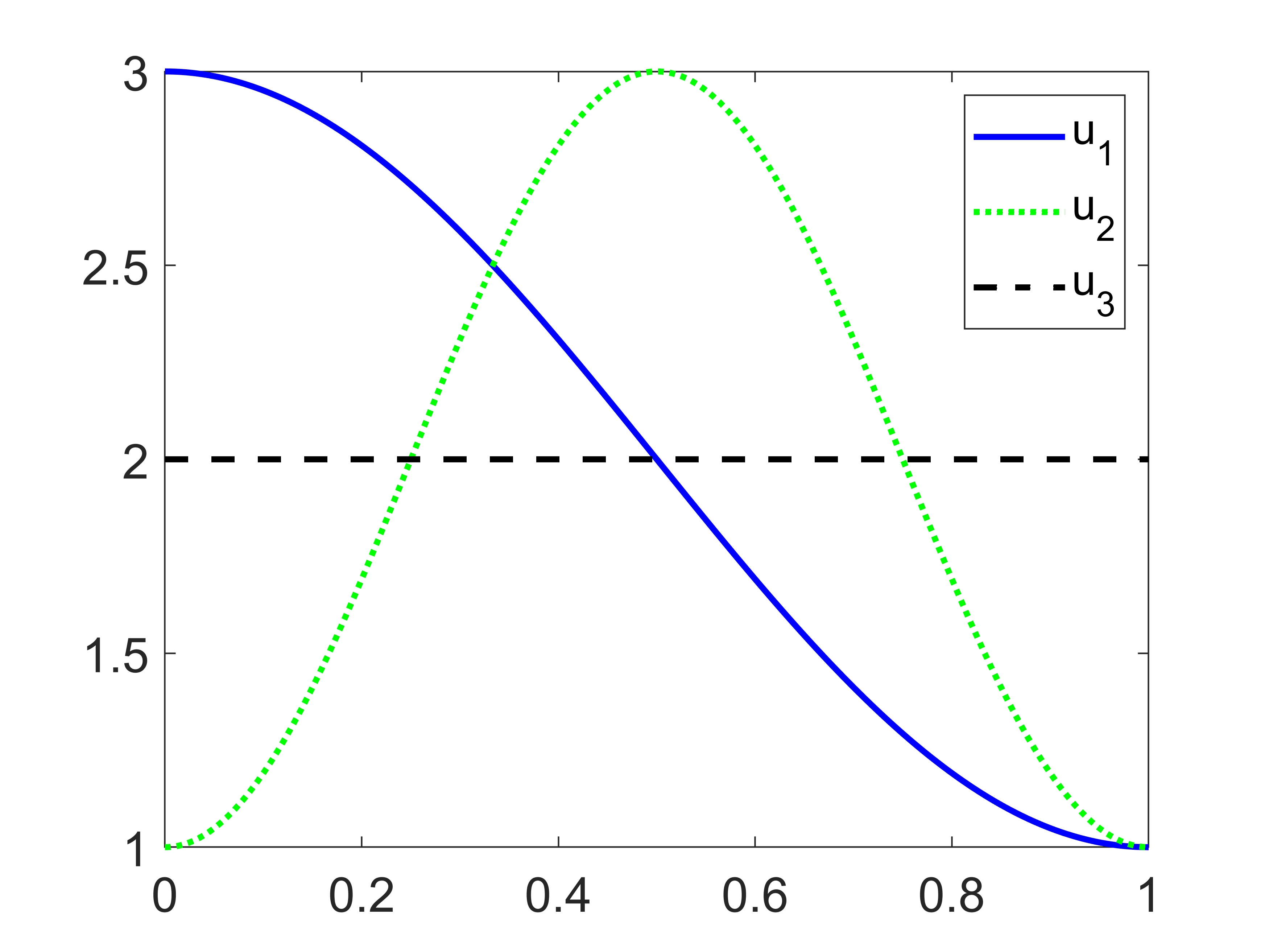
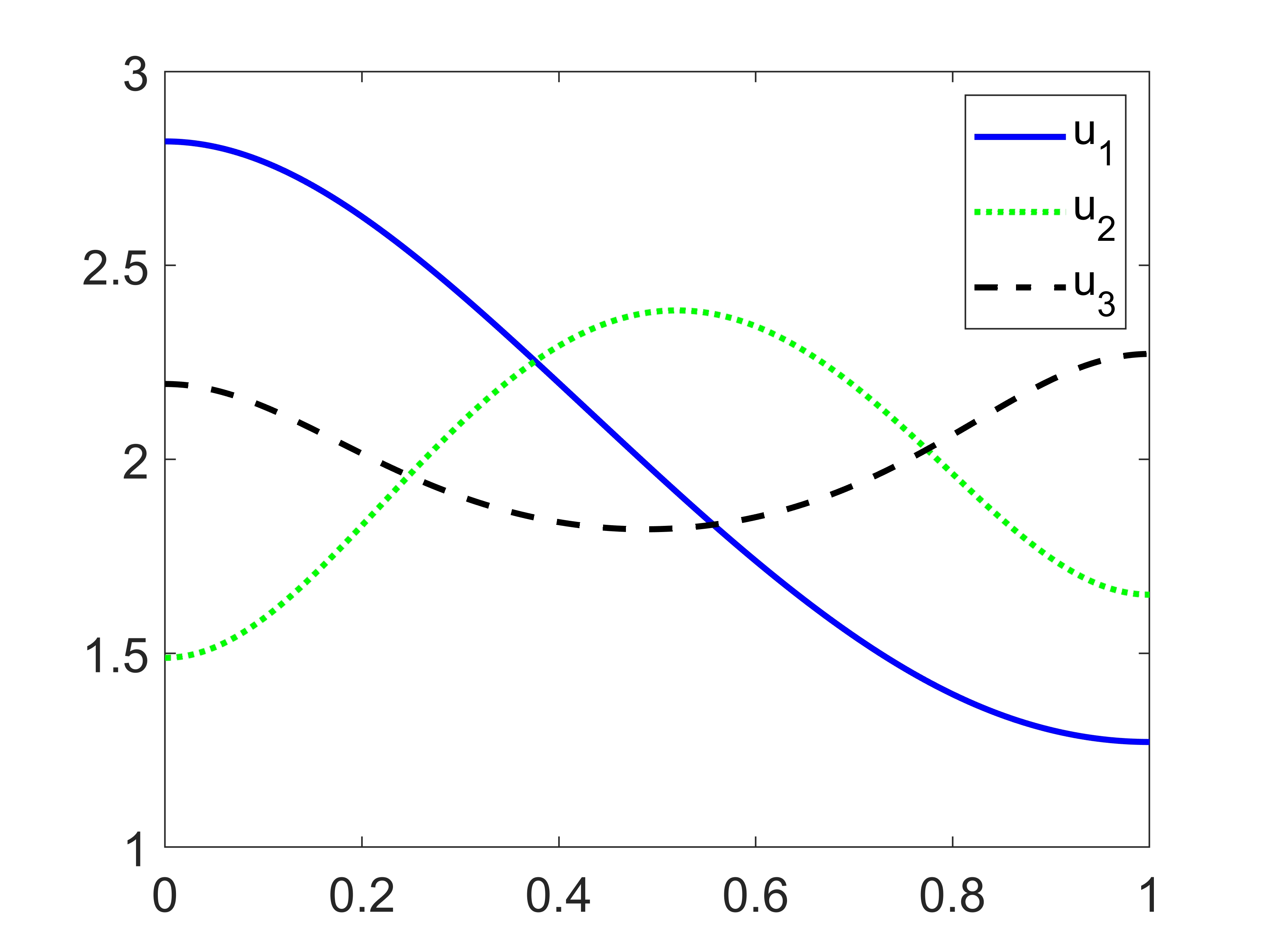
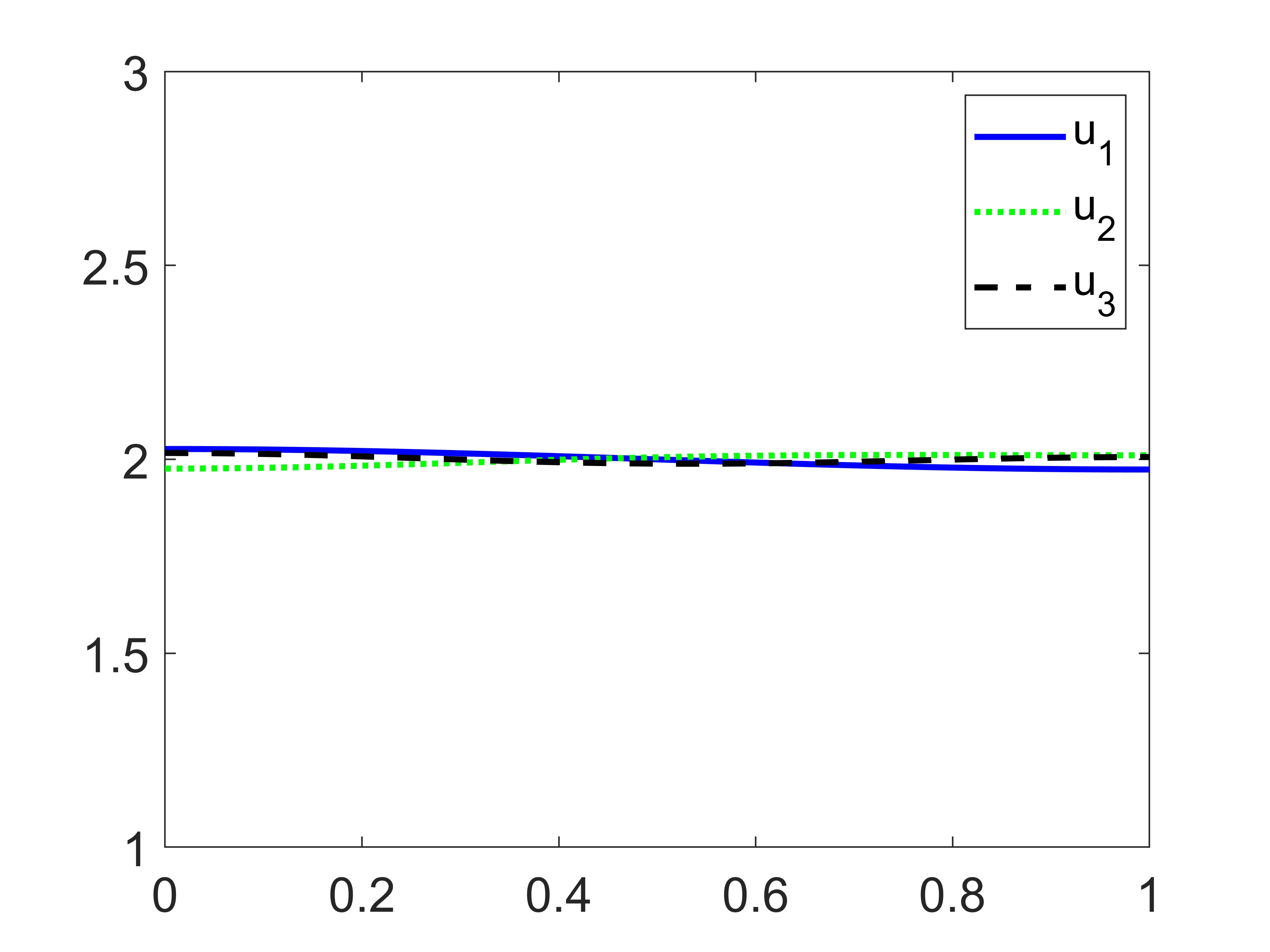
7.2. Second example: two-dimensional domain, two species

We take $\Omega=(0,1)^{2}$, $\Delta x=\sqrt{2}\cdot 2^{-5}\approx 0.0044$, $\Delta t=1/256$, $\gamma=1/2$, and

$$A=\begin{pmatrix}1&1/2\\ 1/2&1\end{pmatrix},\quad u^{0}(x)=\begin{pmatrix}\mathrm{1}_{(0,1/2)^{2}}(x)\\ \mathrm{1}_{(1/2,1)^{2}}(x)\end{pmatrix}.$$

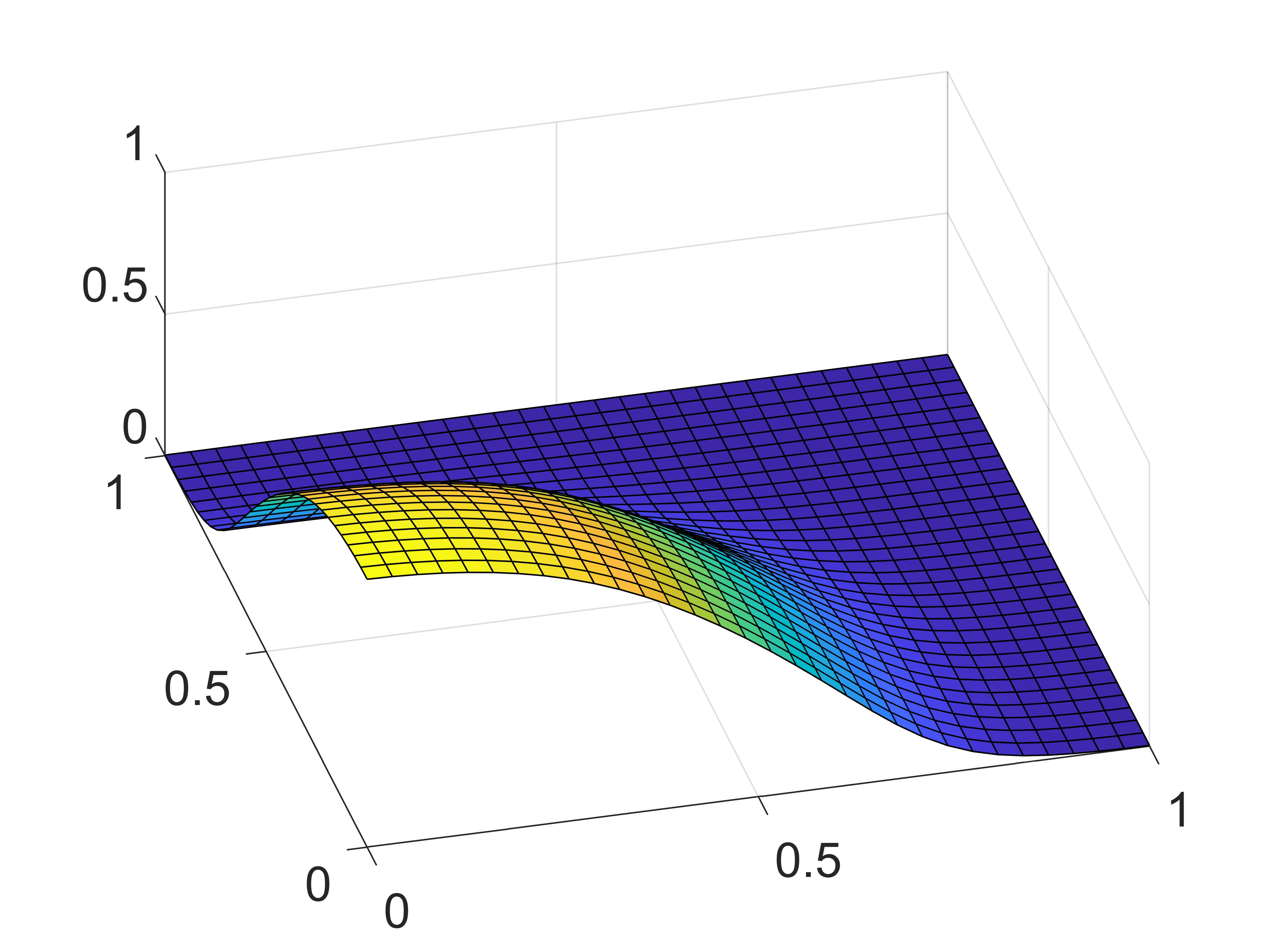
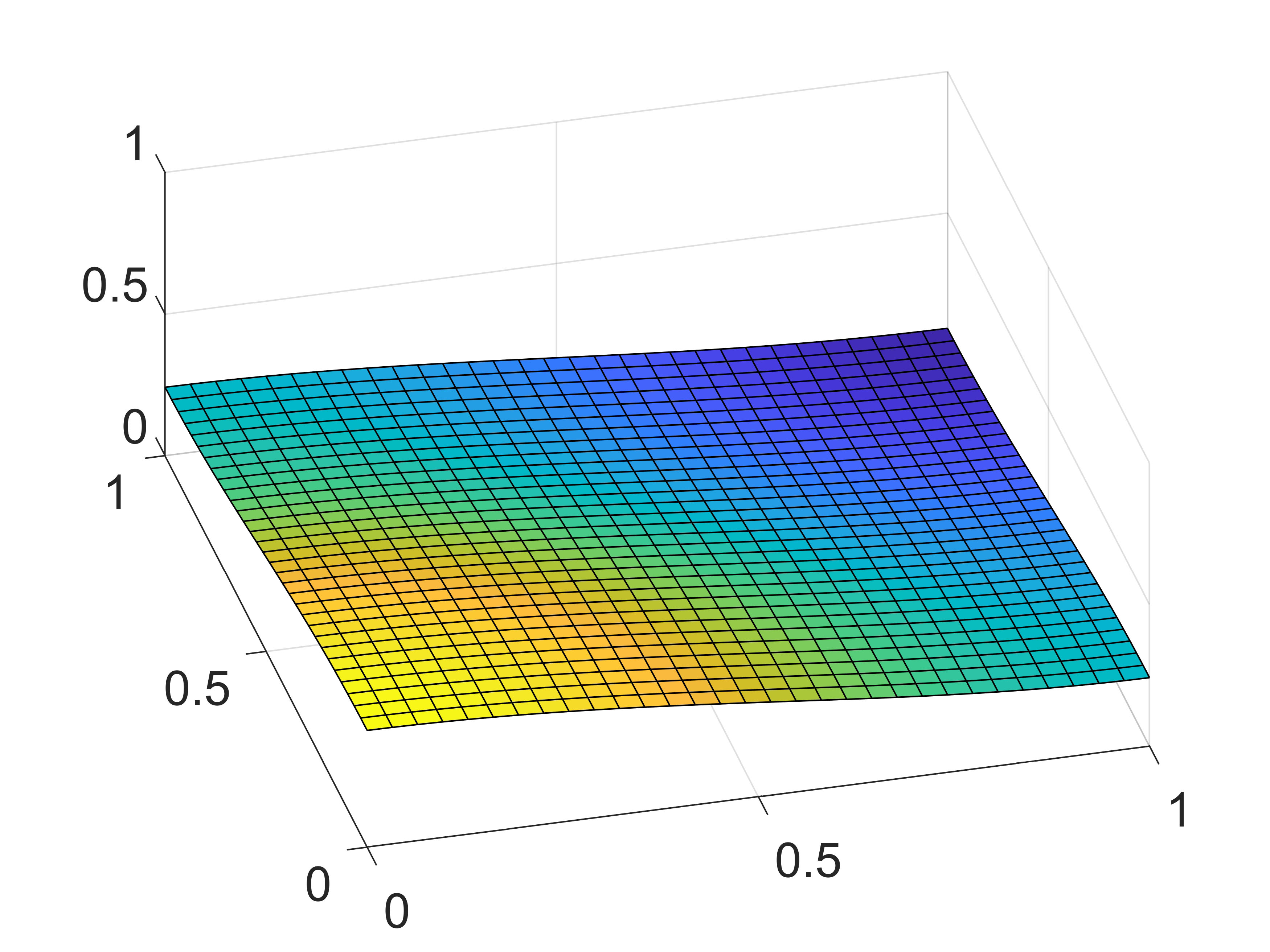
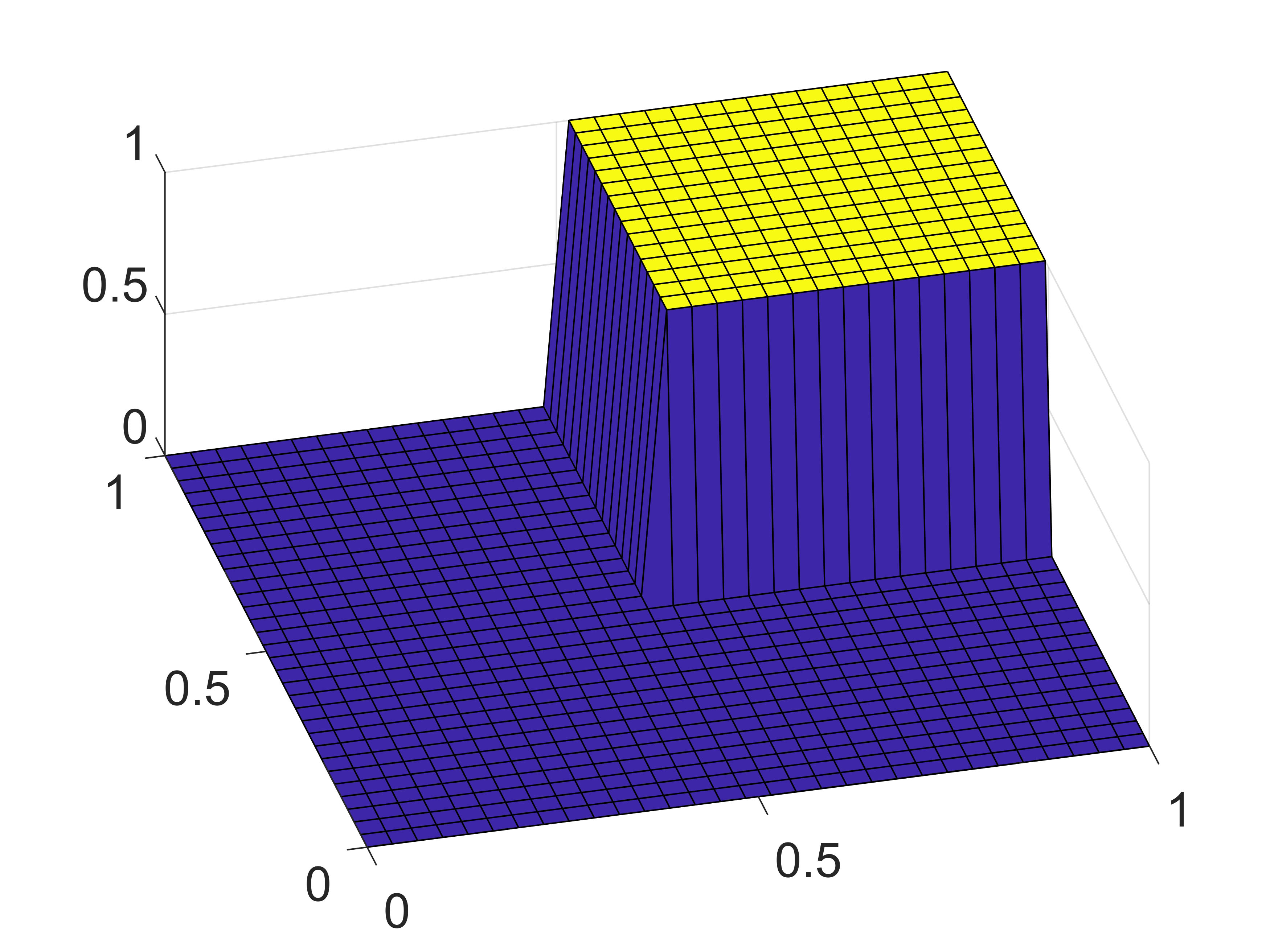
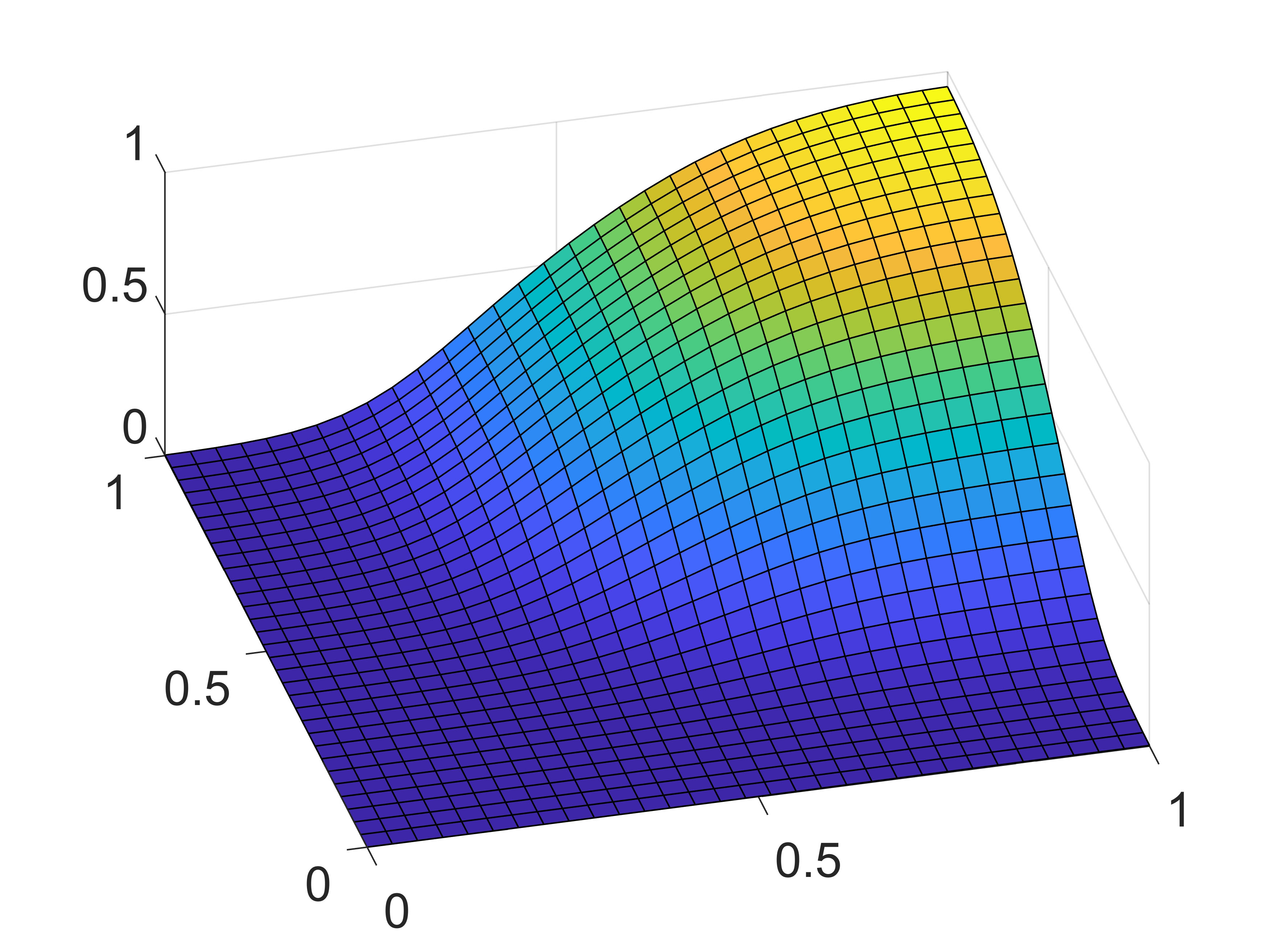
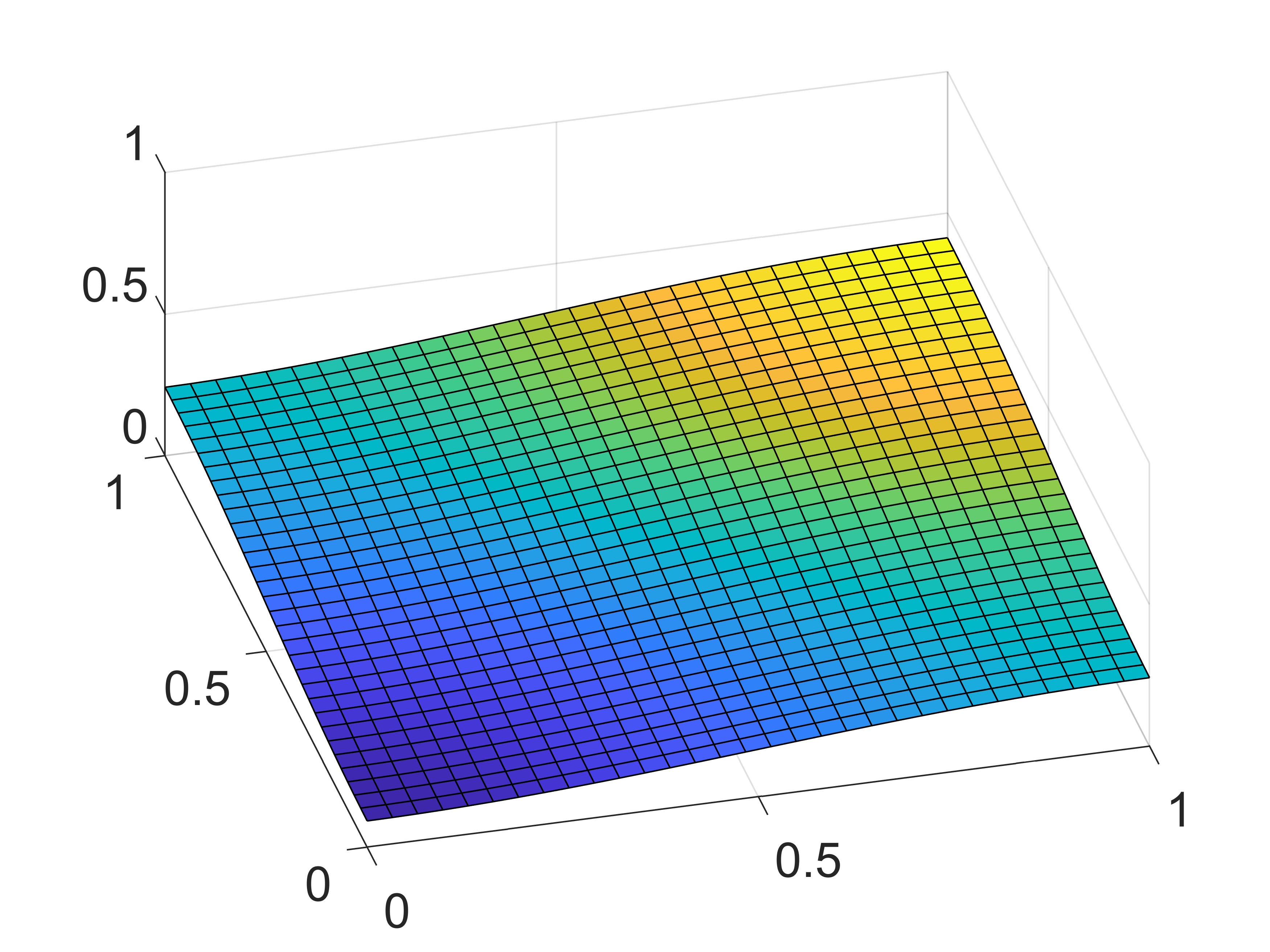
Figure 2 shows the evolution of $u=(u_{1},u_{2})$ at various times. Although being discontinuous and segregated initially, the solution becomes smooth and mixes the densities for positive times. This is not surprising, as full segregation (i.e., the supports of $u_{1}$ and $u_{2}$ do not intersect) is expected only when $\gamma=0$ and $\det A=0$. The numerical scheme preserved the nonnegativity in all our experiments, even for the initial data of this example. The numerical solutions are the same with or without the cutoff used in (18).

Figure 2. Density $u_{1}(t)$ (upper row) and $u_{2}(t)$ (lower row) at times $t=0,0.02,0.2$ (from left to right) versus space.

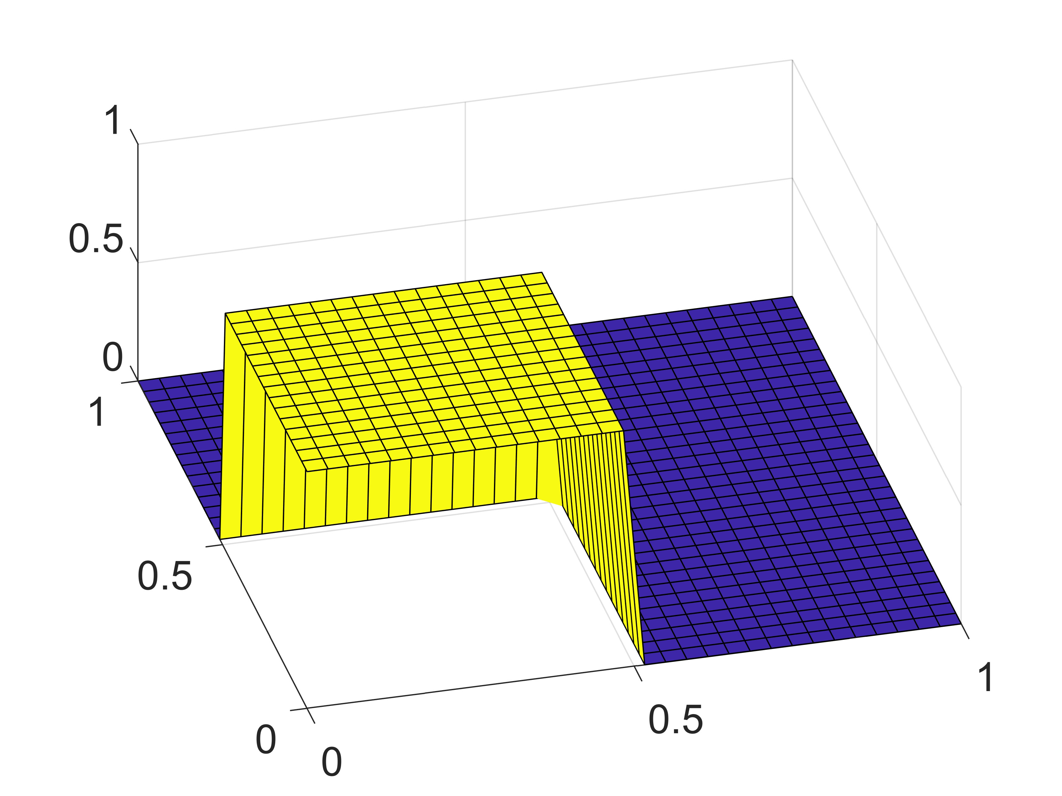
7.3. Third example: exponential time decay

We choose the one-dimensional domain $\Omega=(0,1)$, $\gamma=0.1$, $\Delta x=2^{-7}$, $\Delta t=(10\cdot 2^{7})^{-1}$, and

$$A=\begin{pmatrix}\beta&2\\ 2&1\end{pmatrix},\quad u^{0}(x)=\begin{pmatrix}2-\cos(\pi x)\\ 2+\cos(\pi x)\end{pmatrix},$$

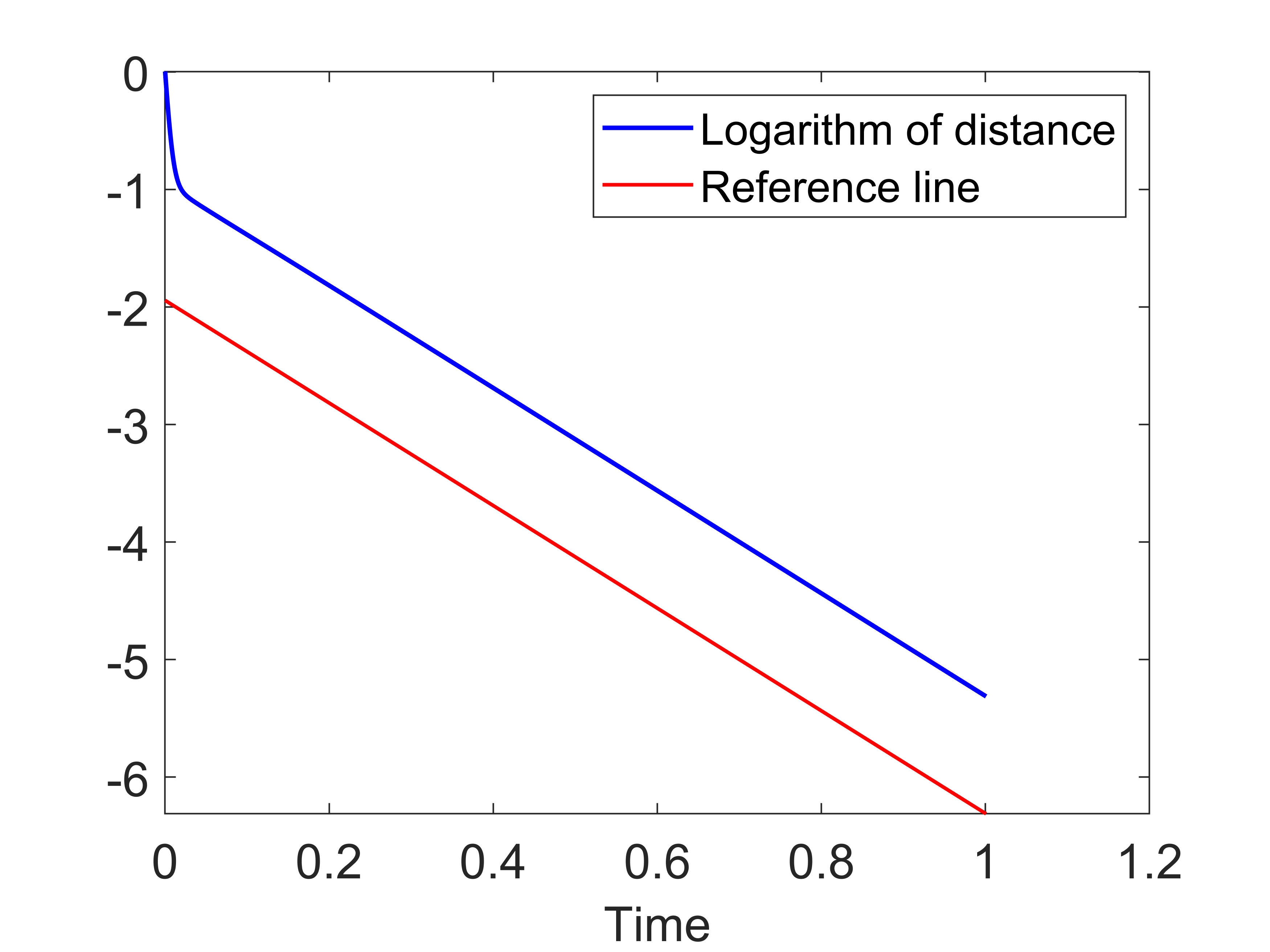
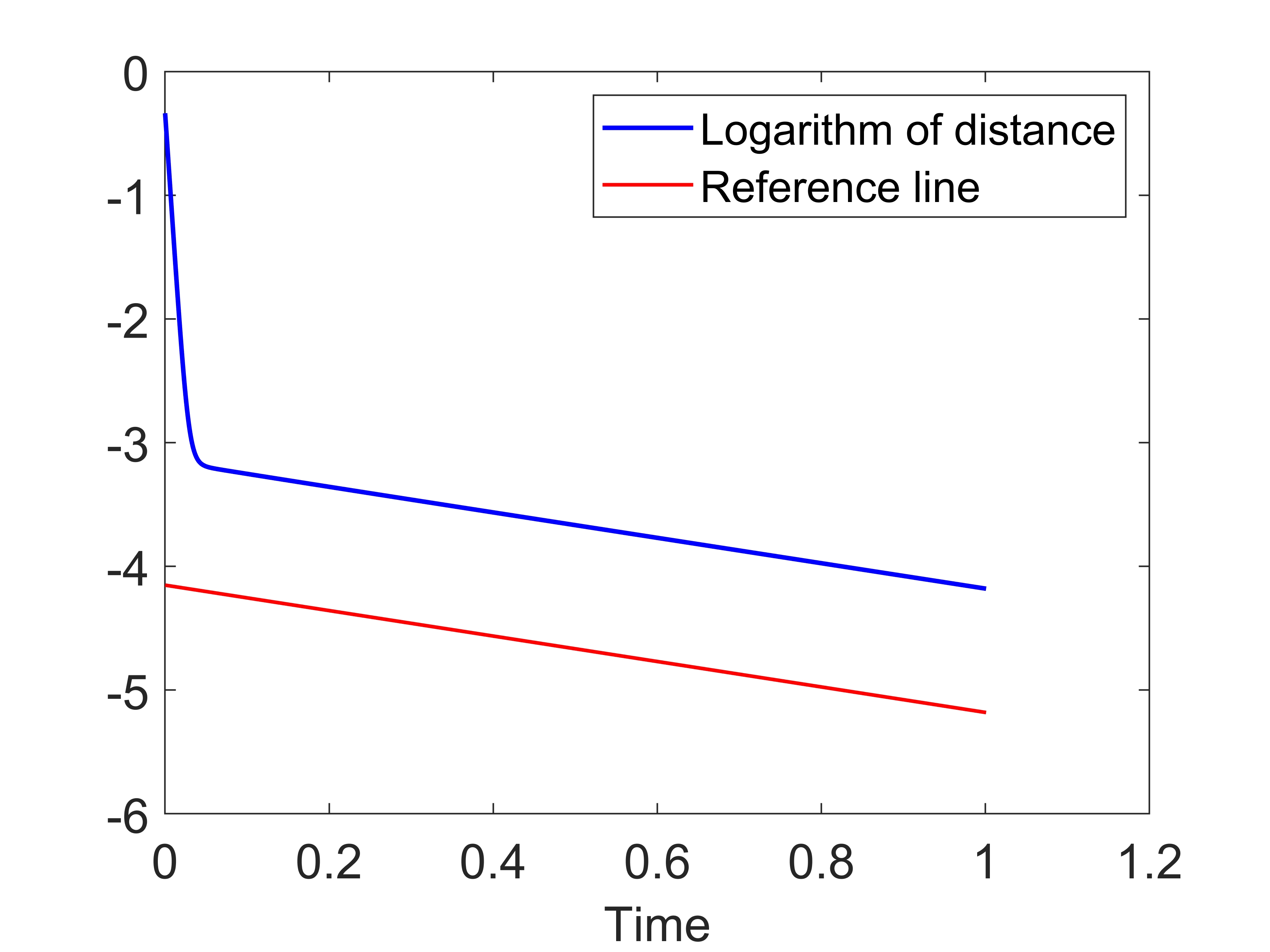
where $\beta>4$. The distance $\|A^{1/2}(u^{k}-\bar{u})\|_{L^{2}(\Omega)}$ presented in Figure 3 for $\beta=5$ and $\beta=4.01$ shows that the time decay behaves exponentially, as predicted by Theorem 4. The decay rates (excluding the initial decay) are $-4.37$ for $\beta=5$ and $-1.03$ for $\beta=4.01$, and they decrease for smaller values of $\det A$. We have also observed an exponential decay when $\gamma=0$ with smaller decay rates.

Figure 3. Semilogarithmic plot for $\|A^{1/2}(u^{k}-\bar{u})\|_{L^{2}(\Omega)}$ versus time $t_{k}$.

7.4. Fourth example: Convergence rate in time

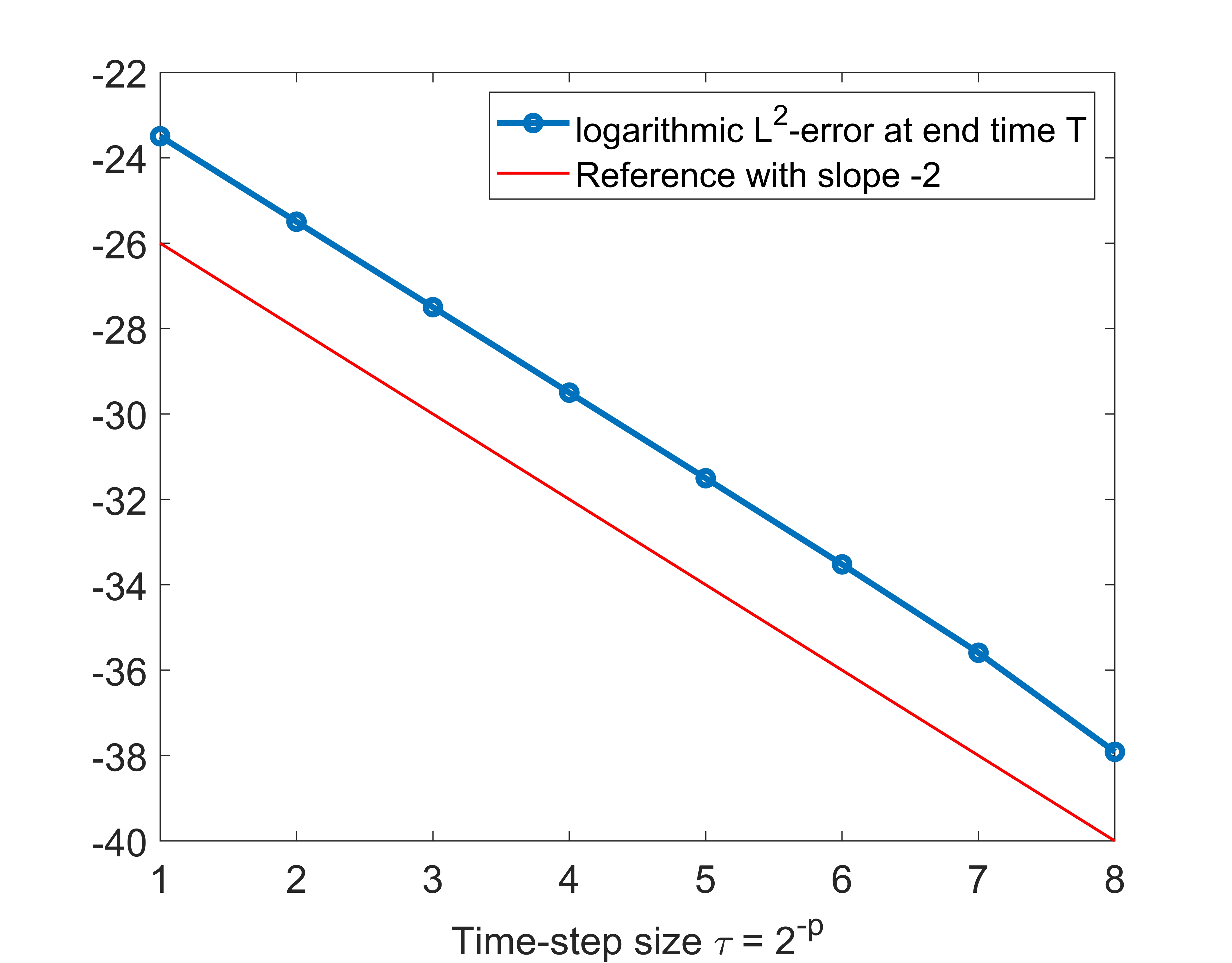
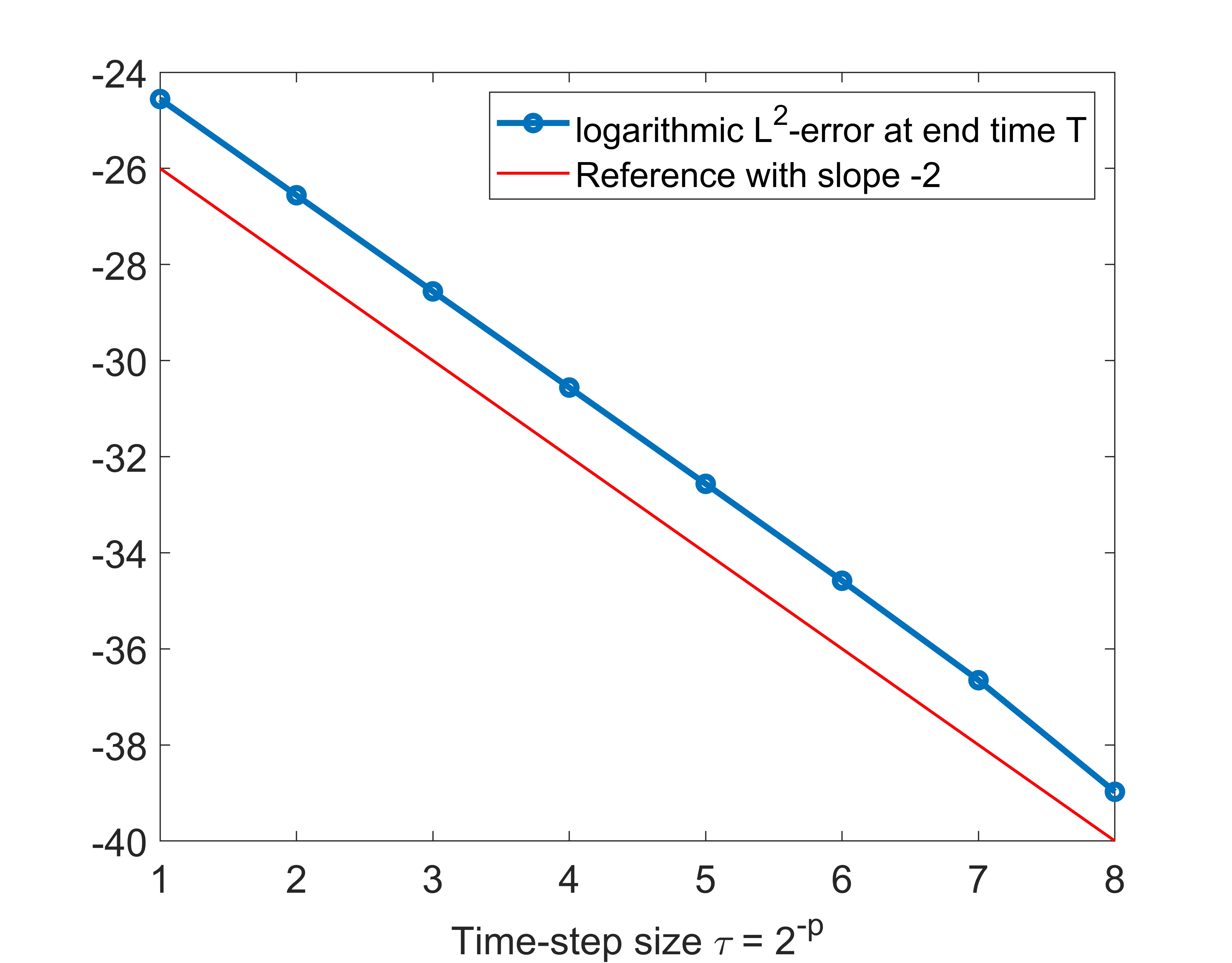
We choose the values for $A$ and $u^{0}$ as in the previous example as well as $\gamma=0$, $\Delta x=2^{-9}$, and $\Delta t=(10\cdot 2^{p})^{-1}$ with $p=1,\ldots,8$. The reference solution $u_{\rm ref}$ is computed with the time step size $\Delta t=(10\cdot 2^{9})^{-1}$. As expected, the convergence rate at time $T=0.02$, shown in Figure 4 for two different values of $\beta$, is about two, even in the case $\det A=0$.

Figure 4. Discrete $L^{2}(\Omega)$ error $\|A^{1/2}(u^{(\Delta t)}-u_{\rm ref})(T)\|_{L^{2}(\Omega)}$ versus time step size $\Delta t=(10\cdot 2^{p})^{-1}$ for $p=1,\ldots,8$ for $\beta=5$ (left) and $\beta=4$ (right).

References

- [1] H. Amann. Nonhomogeneous linear and quasilinear elliptic and parabolic boundary value problems. In: H. J. Schmeisser and H. Triebel (eds.), Funct. Spaces Differ. Op. Nonlin. Anal., pp. 9–126. Teubner, Wiesbaden, 1993.
- [2] B. Andreianov, M. Bendahmane, and R. Ruiz-Baier. Analysis of a finite-volume method for a cross-diffusion model in population dynamics. Math. Models Meth. Appl. Sci. 21 (2011), 307–344.
- [3] R. Bailo, J. A. Carrillo, and J. Hu. Fully discrete positivity-preserving and energy-dissipating schemes for aggregation-diffusion equations with a gradient-flow structure. Commun. Math. Sci. 18 (2020), 1259–1303.
- [4] M. Bertsch, M. Gurtin, D. Hilhorst, and L. Peletier. On interacting populations that disperse to avoid crowding: preservation of segregation. J. Math. Biol. 23 (1985), 1–13.
- [5] M. Bertsch, D. Hilhorst, H. Izuhara, and M. Mimura. A nonlinear parabolic-hyperbolic system for contact inhibition of cell-growth. Differ. Eqs. Appl. 4 (2012), 137–157.
- [6] M. Bessemoulin-Chatard. A finite volume scheme for convection-diffusion equations with nonlinear diffusion derived from the Scharfetter–Gummel scheme. Numer. Math. 121 (2012), 637–670.
- [7] M. Bessemoulin-Chatard, C. Chainais-Hillairet, and F. Filbet. On discrete functional inequalities for some finite volume schemes. IMA J. Numer. Anal. 35 (2015), 1125–1149.
- [8] C. Calgaro and M. Ezzoug. -stability of the IMEX-BDF2 finite volume scheme for convection-diffusion equation. In: C. Cancès and P. Omnes (eds.), Finite Volumes for Complex Applications VIII, pp. 245–253. Springer, Cham, 2017.
- [9] C. Cancès and B. Gaudeul. A convergent entropy diminishing finite volume scheme for a cross-diffusion system. SIAM J. Numer. Anal. 58 (2020), 2684–2710.
- [10] C. Chainais-Hillairet, J.-G. Liu, and Y.-J. Peng. Finite volume scheme for multi-dimensional drift-diffusion equations and convergence analysis. ESAIM Math. Model. Numer. Anal. 37 (2003), 319–338.
- [11] L. Chen, E. Daus, and A. Jüngel. Rigorous mean-field limit and cross diffusion. Z. Angew. Math. Phys. 70 (2019), no. 122, 21 pages.
- [12] X. Chen and A. Jüngel. Weak-strong uniqueness of renormalized solutions to reaction-cross-diffusion systems. Math. Models Meth. Appl. Sci. 29 (2019), 237–270.
- [13] W. Chen, C. Wang, X. Wang, and S. Wise. Positivity-preserving, energy stable numerical schemes for the Cahn–Hilliard equation with logarithmic potential. J. Comput. Phys. X 3 (2019), no. 1000031, 29 pages.
- [14] W. Dahmen, B. Faermann, I. Graham, W. Hackbusch, and S. Sauter. Inverse inequalities on non-quasi-uniform meshes and applications to the Mortar element method. Math. Comput. 73 (2004), 1107–1138.
- [15] L. Dong, C. Wang, H. Zhang, and Z. Zhang. A positivity-preserving second-order BDF scheme for the Cahn–Hilliard equation with variable interfacial parameters. Commun. Comput. Phys. 28 (2020), 967–998.
- [16] M. Dreher and A. Jüngel. Compact families of piecewise constant functions in . Nonlin. Anal. 75 (2012), 3072–3077.
- [17] J. Droniou and N. Nataraj. Improved estimate for gradient schemes and super-convergence of the TPFA finite volume scheme. IMA J. Numer. Anal. 38 (2018), 1254–1293.
- [18] P.-E. Druet, K. Hopf, and A. Jüngel. Hyperbolic-parabolic normal form and local classical solutions for cross-diffusion systems with incomplete diffusion. Submitted for publication, 2022. arXiv:2210.17244.
- [19] E. Emmrich. Two-step BDF time discretization of nonlinear evolution problems governed by monotone operators with strongly continuous perturbations. Comput. Meth. Appl. Math. 9 (2009), 37–62.
- [20] R. Eymard, T. Gallouët, and R. Herbin. Convergence of finite volume schemes for semilinear convection diffusion equations. Numer. Math. 82 (1999), 91–116.
- [21] R. Eymard, T. Gallouët, and R. Herbin. Finite volume methods. In: P. G. Ciarlet and J.-L. Lions (eds.). Handbook of Numerical Analysis 7 (2000), 713–1018.
- [22] Y. Gu and J. Shen. Bound preserving and energy dissipative schemes for porous medium equation. J. Comput. Phys. 410 (2020), no. 109378, 21 pages.
- [23] A. Hill. Global dissipativity for A-stable methods. SIAM J. Numer. Anal. 34 (1997), 119–142.
- [24] A. Jüngel and J.-P. Milišic̀. Entropy dissipative one-leg multistep time approximations of nonlinear diffusive equations. Numer. Meth. Part. Diff. Eqs. 31 (2015), 1119–1149.
- [25] A. Jüngel, S. Portisch, and A. Zurek. Nonlocal cross-diffusion systems for multi-species populations and networks. Nonlin. Anal. 219 (2022), no. 112800, 26 pages.
- [26] A. Jüngel and A. Zurek. A finite-volume scheme for a cross-diffusion model arising from interacting many-particle population systems. In: R. Klöfkorn, E. Keilegavlen, F. Radu, and J. Fuhrmann (eds.), Finite Volumes for Complex Applications IX, pp. 223–231. Springer, Cham, 2020.
-
[27]
A. Jüngel and A. Zurek. A discrete boundedness-by-entropy method for
finite-volume approximations of cross-diffusion systems. To appear in
IMA J. Math. Anal., 2022.
https://doi.org/10.1093/imanum/drab101. - [28] R. Krishna. Uphill diffusion in multicomponent mixtures. Chem. Soc. Rev. 44 (2015), 2812–2836.
- [29] D. Matthes and S. Plazetta. A variational formulation of the BDF2 method for metric gradient flows. ESAIM Math. Model. Numer. Anal. 53 (2019), 145–172.
- [30] C. Rao. Diversity and dissimilarity coefficients: a unified approach. Theor. Popul. Biol. 21 (1982), 24–43.