Construction of fractal functions using Kannan mappings and smoothness analysis

Abstract.

Let $T$ be a self-map on a metric space $(X,d)$. Then $T$ is called Kannan map if there exists $\alpha$, $0<\alpha<\frac{1}{2}$, such that

$$d(T(x),T(y))\leq\alpha[d(x,T(x))+d(y,T(y))],~{}~{}\text{for all}~{}x,y\in X.$$

This paper aims to introduce a new method to construct fractal functions using Kannan mappings. First, we give the rigorous construction of fractal functions with the help of the Kannan iterated function system (IFS). We also show the existence of a Borel probability measure supported on the attractor of the Kannan IFS satisfying the strong separation condition. Moreover, we study the smoothness of the constructed fractal functions. We end the paper with some examples and graphical illustrations.

1. INTRODUCTION

The concept of fractal interpolation function (FIF) was introduced by Barnsley [2, 3] through iterated function system (IFS), and their construction is rooted in the theory of IFS [9]. The FIF is an interpolation function whose graph is an invariant set of an IFS. The pioneering research on fractal interpolation has gotten much attention in the literature, and it continues to flourish. The concept of FIF has been extended and generalized in several ways given in the literature. Wang and Yu [27] gave the construction of new class IFSs with variable parameters and generated associated FIFs. Also, they studied the smoothness and stability of FIFs under some conditions on data points. The construction of nonlinear FIF using Matkowski and the Rakotch fixed point theorems is given in [20]. In this order, Songli [21] gave the construction of nonlinear FIF on Sierpiński gasket. The reader may refer to books [3, 16] for the details on fractal functions. The fractal dimension is one of the major themes in fractal geometry. Many works on the fractal dimensions of fractals functions are in the literature. There are various approaches, such as the mass-distribution principle, potential theory, Fourier transform, positive operators, etc., to compute or estimate the Hausdorff dimension of a set [11, 26]. Using the potential theoretic approach, Barnsley gave results on the Hausdorff dimension of an affine FIF in [3]. Falconer [11] also gave the estimate of the Hausdorff dimension of an affine FIF. The results on the Hausdorff dimension using the positive operators approach are given in [26]. Priyadarshi [19] gave an algorithm to determine lower bounds for the Hausdorff dimension of a set of complex continued fractions and estimated the best lower bound. Jha and Verma [12] established very interesting results for fractal dimensions of fractal functions and some invariant sets. They estimated fractal dimensions for a class of FIFs, widely known as $\alpha$-fractal functions, by using function spaces such as Hölder space, oscillation space, and space of bounded variation. Ruan et al. [22] estimated the box dimension of the new class of linear FIFs by using the $\delta$-covering method. Additionally, they have established a relationship between the order of fractional integral and box dimensions of two linear FIFs. As we know, recurrent FIF is the generalization of linear FIF, and the graph of recurrent FIF is the invariant set of recurrent IFS. Barnsley and Massopust [4] gave results on the bilinear FIFs and their box dimension. Few recent developments on fractal dimensions can be seen in [6, 24, 25]. Cheng et al. [6] introduced the notion of upper metric mean dimension with potential on any subset via Carathéodory-Pesin structures. Selmi [24] studied the multifractal Hausdorff and packing dimensions of Borel probability measures and studied their behaviors under orthogonal projections. In this order, Selimi estimated the multifractal Hausdorff and the packing dimensions of product measures in [25].
Barnsley [2, 3] considered the collection of self-contraction mappings and used the Hutchinson operator and Banach fixed point principle to construct fractal functions. Kannan [13, 14] introduced a new fixed point theorem widely known as Kannan fixed point theorem. Other related results on Kannan mapping can be seen in [8, 10]. By using the concept of Kannan mapping, Sahu et al. [23] introduced the notion of the Kannan iterated function system.

Theorem 1.1.

[14] Let $T$ is a map of the complete metric space $X$ into itself and if

$$d(T(x),T(y))\leq\alpha[d(x,T(x))+d(y,T(y))],~{}\forall~{}x,y\in X,~{}0<\alpha<\frac{1}{2}.$$

Then $T$ has the unique fixed point in $X.$

A natural question arises can we construct fractal functions using the concept of Kannan fixed point theory? This question motivates us to conduct the current study. In this study, we use the concept of Kannan IFS and Kannan fixed point theorem and derive very interesting results.
This paper is organized as follows: Section 2 is devoted to preliminaries and required terminologies related to this article. Section 3 presents the construction of fractal functions and the existence of self-similar measures. In Section 4, the smoothness result of the Kannan fractal function is given. The graphical illustration of the Kannan fractal functions is given in Section 5.

2. Background and preliminaries

This section aims to provide some basic definitions and results that act as prelude to this article. Let $F\neq\emptyset$ be a subset of $\mathbb{R}^{n}.$ The diameter of $F$ is given by

$$\text{diam}_{d}(F)=\sup\left\{d(x,y):x,y\in F\right\}.$$

If $\{F_{i}\}$ is a countable (or finite) collection of sets having a diameter at most $\delta$ which cover set $E\subseteq\mathbb{R}^{n},$ then we say that $\{F_{i}\}$ is a $\delta$-cover of $E.$ For $\delta>0$ and a non-negative real number $s$, we define

$$H_{\delta,d}^{s}(E)=\inf\left\{\sum_{i=1}^{\infty}\text{diam}_{d}(F_{i})^{s}:\{F_{i}\}~{}\text{is a}~{}\delta-\text{cover of}~{}E\right\}.$$

Definition 2.1.

The $s$-dimensional Hausdorff measure of set $E$ is given by $H^{s}(E)=\lim_{\delta\to 0}H_{\delta}^{s}(E).$

Definition 2.2.

( Hausdorff dimension) Let $s\geq 0$ and $E\subseteq\mathbb{R}^{n}.$ The Hausdorff dimension of $E$ is defined as

$$\dim_{H}(E)=\inf\{s:H^{s}(E)=0\}=\sup\{s:H^{s}(E)=\infty\}.$$

Definition 2.3.

(Box Dimension) Let $E\subseteq\mathbb{R}^{n}$ be bounded and non-empty and let $N_{\delta}(E)$ be the smallest number of sets of diameter at most $\delta$ which cover $E.$ The lower box dimension of $E$ is

$$\underline{\dim}_{B}(E)=\mathop{\underline{\lim}}_{\delta\to 0}\frac{\log N_{\delta}(E)}{-\log\delta},$$

and the upper box dimension of $E$ is

$$\overline{\dim}_{B}(E)=\overline{\lim_{\delta\to 0}}\frac{\log N_{\delta}(E)}{-\log\delta},$$

If both lower and upper box dimensions are the same, then that quantity is called the box dimension of $E$ and it is given by

$$\dim_{B}(E)=\lim_{\delta\rightarrow 0}\frac{\log N_{\delta}(E)}{-\log\delta}.$$

For the details on the Hausdorff and box dimensions, the reader may be referred to [11].

Definition 2.4.

Let $d_{1}$ and $d_{2}$ are two matrices on $X$, then $d_{1}$ and $d_{2}$ are topologically equivalent if and only if

$$d_{1}(x_{n},x)\to 0\Longleftrightarrow d_{2}(x_{n},x)\to 0,$$

for $\{x_{n}\}\subset X$ and $x\in X.$
Let $d_{1}$ and $d_{2}$ are two matrices on $X$, then $d_{1}$ and $d_{2}$ are metrically equivalent if and only if there exists $c_{1},c_{2}>0$ and $x,y\in X$ such that

$$c_{1}d_{1}(x,y)\leq d_{2}(x,y)\leq c_{2}d_{1}(x,y).$$

Fractal Interpolation Function

Now, we introduce FIF in brief. Here, we consider a set for interpolation as $\{(x_{n},y_{n}):n=1,2,\dots,N\}$. We set $J=\{1,2,...,N-1\}$, $I=[x_{1},x_{N}]$ and for $j\in J$, let $I_{j}=[x_{j},x_{j+1}]$. For $j\in J$, let $L_{j}:I\rightarrow I_{j}$ be a contractive homomorphism such that

$$L_{j}(x_{1})=x_{j},L_{j}(x_{N})=x_{j+1},j\in J.$$

Now, define $F_{j}:K=I\times\mathbb{R}\rightarrow\mathbb{R},j\in J$, which is a contraction in the second variable, that is, $|F_{j}(x,y)-F_{j}(x,y^{\prime})|\leq r_{j}|y-y^{\prime}|,$ for all $x\in I$, $r_{j}\in[0,1)$ and $y,y^{\prime}\in\mathbb{R}$ and satisfying $F_{j}(x_{1},y_{1})=y_{j},F_{j}(x_{N},y_{N})=y_{j+1},j\in J.$ We shall take

(2.1) $$L_{j}(x)=a_{j}x+b_{j}~{}F_{j}(x,y)=\alpha_{j}y+q_{j}(x),$$

In the above expression $a_{j}$ and $b_{j}$ are determined by using conditions $L_{j}(x_{1})=x_{j},L_{j}(x_{N})=x_{j+1}.$ Here, $\alpha_{j}$ is the scaling factor with $|\alpha_{j}|<1$ and continuous functions $q_{j}:I\rightarrow\mathbb{R},j\in J$ satisfy “join-up conditions” imposed for the bivariate maps $F_{j}$. That is, $q_{j}(x_{1})=y_{j}-\alpha_{j}y_{1}$ and $q_{j}(x_{N})=y_{j+1}-\alpha_{j}y_{N}$ for all $j\in J$. Now define functions $W_{j}:I\times\mathbb{R}\rightarrow I\times\mathbb{R}$ for $j\in J$ by

$$W_{j}(x,y)=\big{(}L_{j}(x),F_{j}(x,y)\big{)}.$$

Theorem $1$ in [3] says that the IFS $\mathcal{I}:=\{I\times\mathbb{R};W_{1},W_{2},\dots,W_{N-1}\}$ defined above has a unique attractor which is the graph of a function $f$ which satisfies the following functional equation reflects self-referentiality:

$$f(x)=\alpha_{j}f\big{(}L_{j}^{-1}(x)\big{)}+q_{j}\big{(}L_{j}^{-1}(x)\big{)},x\in I_{j},j\in J.$$

The above function $f$ is known as the fractal interpolation function.

Kannan mapping

In 1969, Kannan [13] introduced a mapping, which was an improvement over the contraction mapping, known as Kannan mapping, defined as follows:

If there exists a number $\alpha$, $0<\alpha<\frac{1}{2}$, such that, for all $x,y\in X,$

$$d(T(x),T(y))\leq\alpha[d(x,T(x))+d(y,T(y))].$$

Then $T$ is called a Kannan mapping and $\alpha$ is called Kannan-contractivity factor of $T$. Let $T_{n}:X\to X$ are Kannan mappings having contractivity factor $\alpha_{n},$ for $n=1,2,\dots,N$ and $(X,d)$ be a complete metric space. Then, the set $\{X;T_{n},n=1,2,\dots,N\}$ is said to be Kannan IFS.

Remark 2.5.

Let $f:[0,1]\to[0,1]$ be defined by $f(x)=\frac{x}{3}.$ Then this function $f$ is a contraction mapping with contraction factor $\frac{1}{3},$ but it is not a Kannan mapping. On the other hand, the function $g:[0,1]\to[0,1]$ defined by

$$g(x)=\begin{cases}\frac{x}{4},\quad~{}\text{if}~{}~{}0\leq x<\frac{1}{2}\\ \frac{x}{5},~{}\quad\text{if}~{}~{}~{}~{}\frac{1}{2}\leq x\leq 1.\end{cases}$$

is a Kannan mapping with $\beta=\frac{4}{9}$ but it is not a contraction mapping. The concepts of the Kannan operator and contraction are independent. The self-map $T$ given in the previous example is Kannan, but it is not a contraction due to its discontinuity.

The following simple note can be seen in [10]. However, we include its details for the reader’s convenience.

Note 2.6.

Let $(X,d)$ be a metric space and $T:X\to X$ is contraction with constant $c<\frac{1}{3}.$ Then $T$ is Kannan contractive with respect to metric $d$.
Because of the contractivity of $T$, we have

$$d(T(x_{1}),T(x_{2}))\leq cd(x_{1},x_{2})\leq cd(x_{1},Tx_{1})+cd(Tx_{1},Tx_{2})+c(Tx_{2},x_{2}),~{}\forall~{}x_{1},x_{2}\in X.$$

This turns

$$d(T(x_{1}),T(x_{2})) \leq\alpha[d(x_{1},T(x_{1}))+d(x_{2},T(x_{2}))],~{}\forall~{}x_{1},x_{2}\in X.$$

Since $0<\alpha:=\frac{c}{1-c}<\frac{1}{2},$ $T$ is a Kannan mapping.

Proposition 2.7.

Let $X$ be a complete metric space and $d_{1}$ and $d_{2}$ are equivalent metrics on $X$, i.e., there exist positive constants $c_{1},c_{2}$ such that

$$c_{1}d_{1}(x_{1},x_{2})\leq d_{2}(x_{1},x_{2})\leq c_{2}d_{1}(x_{1},x_{2}),~{}~{}x_{1},x_{2}\in X.$$

If $T$ is a contraction on $X$ with respect to the metric $d_{1}$ then there exists an $m\in\mathbb{N}$ such that $T^{m}$ is a Kannan contraction with respect to the metric $d_{2}$.

Proof.

Since $T$ is contraction on $(X,d_{1})$, there exits $0\leq k<1$ such that

$$d_{1}(Tx_{1},Tx_{2})\leq kd_{1}(x_{1},x_{2}),~{}~{}x_{1},x_{2}\in X.$$

Whence $d_{2}(Tx_{1},Tx_{2})\leq c_{2}d_{1}(Tx_{1},Tx_{2})\leq c_{2}kd_{1}(x_{1},x_{2})\leq\Bigg{(}\frac{c_{2}}{c_{1}}k\Bigg{)}d_{2}(x_{1},x_{2}).$ Take $m\in\mathbb{N}$ such that $\frac{c_{2}}{c_{1}}k^{m}<\frac{1}{3}.$ Then

$$d_{2}(T^{m}x_{1},T^{m}x_{2})\leq c_{2}d_{1}(T^{m}x_{1},T^{m}x_{2})\leq c_{2}k^{m}d_{1}(x_{1},x_{2})\leq\Bigg{(}\frac{c_{2}}{c_{1}}k^{m}\Bigg{)}d_{2}(x_{1},x_{2}).$$

Hence, $T^{m}$ is a contraction with respect to the metric $d_{2}$. From Note 2.6, we conclude that $T^{m}$ is a Kannan contraction with respect to the metric $d_{2}$. Thus, the proof is completed. ∎

Theorem 2.8.

[14] Let $T$ is a map of the complete metric space $X$ into itself and if

$$d(T(x),T(y))\leq\alpha[d(x,T(x))+d(y,T(y))],~{}\forall~{}x,y\in X,~{}0<\alpha<\frac{1}{2}.$$

Then $T$ has the unique fixed point in $X.$

The Hausdorff distance from the set $A$ to the set $B$ is defined as

$$h(A,B)=\max\{\sup_{a\in A}\inf_{b\in B}d(a,b),\sup_{b\in B}\inf_{a\in A}d(a,b)\}.$$

Note 2.9.

In [23, Lemma $3.5$] the authors claimed that for all $B,C\in\mathcal{H}(X),$

$$h(T(B),T(C))\leq\beta[h(B,T(B))+h(C,T(C))].$$

The above claim is not true, for instance, see the following example, which is borrowed from [8].

Example 2.10.

Let $X=\{0,1,2\}$, and the function $d:X\times X\to\mathbb{R}$ and the map $f:X\to X$ be given by

$$d(0,0)=d(1,1)=d(2,2)=0$$

$$d(0,1)=d(1,0)=5,~{}d(1,2)=d(2,1)=2,~{}d(0,2)=d(2,0)=3$$

$$f(1)=f(2)=2,~{}f(0)=1.$$

Then the map $f:X\to X$ is Kannan on $(X,d)$ with contractivity factor $\alpha\in[\frac{2}{5},\frac{1}{2})$ but the map $T:\mathcal{H}(X)\to\mathcal{H}(X)$ given by $T(B)=\cup_{x\in B}f(x)$ for all $B\in\mathcal{H}(X)$ is not a Kannan map on $(\mathcal{H}(X),h(d))$ for any contractivity factor $\alpha\in[0,\frac{1}{2}).$

Remark 2.11.

The above example does not work for the following lemma due to different contractive factors. Here, we correct Lemma $3.5$ of [23], and we show that it holds under certain additional conditions.

Lemma 2.12.

Suppose $T:X\to X$ be a continuous Kannan mapping on the metric space $(X,d)$ with contractivity factor $0<\beta<\frac{1}{6}$. Then $T:\mathcal{H}(X)\to\mathcal{H}(X)$ given by $T(B)=\{T(x):x\in B\}$ for every $B\in\mathcal{H}(X)$ is Kannan mapping on $(\mathcal{H}(X),h(d))$ with contractivity factor $0<\gamma=\frac{\beta}{(1-4\beta)}<\frac{1}{2}$.

Proof.

Let us first recall a basic real-analysis result that the image of a compact set under a continuous map is compact. Since $T$ is continuous, it maps $\mathcal{H}(X)$ into itself. Now, since $T$ is Kannan mapping on $(X,d)$, for $x,y\in X$, we have

$$d(T(x),T(y)) \leq\beta[d(x,T(x))+d(y,T(y))]$$

$$\leq\beta[d(x,T(y))+d(T(y),T(x))+d(y,T(x))+d(T(x),T(y))]$$

$$=\beta[d(x,T(y))+d(y,T(x))]+2\beta d(T(x),T(y)).$$

So, we obtain

$$d(T(x),T(y))\leq\frac{\beta}{(1-2\beta)}[d(x,T(y))+d(y,T(x))].$$

Now, for $B,C\in\mathcal{H}(X)$

$$\sup_{x\in B}\inf_{y\in C}d(T(x),T(y))\leq\frac{\beta}{(1-2\beta)}[\sup_{x\in B}\inf_{y\in C}d(x,T(y))+\sup_{x\in B}\inf_{y\in C}d(y,T(x))].$$

That is,

$$\sup_{x\in B}\inf_{y\in C}d(T(x),T(y))\leq\frac{\beta}{(1-2\beta)}[h(B,T(C))+h(C,T(B))].$$

Thanks to the triangle inequality,

$$h(T(B),T(C))\leq\frac{\beta}{(1-2\beta)}[h(B,T(B))+h(T(B),T(C))$$

$$+h(C,T(C))+h(T(C),T(B))].$$

Consequently,

$$\Big{(}1-\frac{2\beta}{(1-2\beta)}\Big{)}h(T(B),T(C))\leq\frac{\beta}{(1-2\beta)}[h(B,T(B))+h(C,T(C))].$$

Therefore,

$$h(T(B),T(C))\leq\gamma[h(B,T(B))+h(C,T(C))],$$

where $\gamma=\frac{\beta}{(1-4\beta)}<\frac{1}{2}$ for $0<\beta<\frac{1}{6}.$ This completes the proof. ∎

Theorem 2.13.

For a complete metric space $(X,d)$, let $T_{n}:n=1,2,...,N$ are continuous Kannan mappings on $(\mathcal{H}(X),h)$ with contractivity factor $0<\beta_{n}<\frac{1}{6}$, for all $n.$ Define $\mathcal{T}:\mathcal{H}(X)\to\mathcal{H}(X)$ by $\mathcal{T}(B)=\cup_{n=1}^{N}T_{n}(B)$ for each $B\in\mathcal{H}(X).$ Then $\mathcal{T}$ is a Kannan mapping with contractivity factor $\gamma=\max\{\gamma_{n}:n=1,2,...,N\}.$

Proof.

For $B,C\in\mathcal{H}(X)$, we have

$$h(\mathcal{T}(B),\mathcal{T}(C)) =h(T_{1}(B)\cup T_{2}(B)\cup\dots\cup T_{n}(B),T_{1}(C)\cup T_{2}(C)\cup\dots\cup T_{n}(C))$$

$$\leq\max\{h(T_{1}(B),T_{1}(C)),h(T_{2}(B),T_{2}(C)),\dots,h(T_{n}(B),T_{n}(C))\}.$$

By using the above lemma, we obtain

$$h(\mathcal{T}(B),\mathcal{T}(C))$$

$$=\max\bigg{\{}\frac{\beta_{1}}{1-4\beta_{1}}[h(B,T_{1}(B))+h(C,T_{1}(C))],\frac{\beta_{2}}{1-4\beta_{2}}[h(B,T_{2}(B))$$

$$+h(C,T_{2}(C))],\dots,\frac{\beta_{n}}{1-4\beta_{n}}[h(B,T_{n}(B))+h(C,T_{n}(C))]\bigg{\}}$$

$$\leq\max_{1\leq i\leq n}\bigg{\{}\frac{\beta_{i}}{1-4\beta_{i}}\bigg{\}}[\max\{h(B,T_{1}(B)),h(B,T_{2}(B)),...,h(B,T_{n}(B))\}$$

$$+\max\{h(C,T_{1}(C)),h(C,T_{2}(C)),...,h(C,T_{n}(C))\}]$$

$$\leq\max_{1\leq i\leq n}\{\gamma_{i}\}[h(B,T_{1}(B)\cup T_{2}(B))\dots\cup T_{n}(B)+h(C,T_{1}(C)\cup T_{2}(C))\dots\cup T_{n}(C)]$$

$$\leq\gamma[h(B,\mathcal{T}(B))+h(C,\mathcal{T}(C))],$$

where $\gamma=\max_{1\leq i\leq n}\{\gamma_{i}\}=\max_{1\leq i\leq n}\bigg{\{}\frac{\beta_{i}}{1-4\beta_{i}}\bigg{\}}<\frac{1}{2}.$ Hence, $\mathcal{T}$ is Kannan with contractivity factor $\gamma.$ ∎

Remark 2.14.

In [8] Dung et al. proposed a question, whether their results are true or not for $n\geq 3.$ In this order, in the above theorem, we show that $\mathcal{T}$ is Kannan for all $n$. Moreover, from Theorem 2.8, $\mathcal{T}$ has a unique fixed point.

We use the following notations throughout the article: $C(I)$ denotes the set of continuous functions $f:I=[x_{0},x_{N}]\to[a,b].$ Let $C^{*}(I)\subset C(I)$ and given by $C^{*}=\{f\in C(I):f(x_{0})=y_{0},f(x_{N})=y_{n}\}.$ $K=I\times\mathbb{R}.$
Let us define a metric $d_{\theta}$ on $K$ as follows

$$d_{\theta}((x,y),(z,w))=|x-z|+\theta|y-w|,~{}\theta>0.$$

Note that $(\mathcal{C}^{*}(I),\mathcal{H}_{\theta})$ is a complete metric space with respect to Hausdorff metric $\mathcal{H}_{\theta}$, where

$$\mathcal{H}_{\theta}(f,g)=\mathcal{H}_{\theta}(G_{f},G_{g})=\max\{\sup_{x\in G_{f}}\inf_{y\in G_{g}}d_{\theta}(x,y),\sup_{y\in G_{g}}\inf_{x\in G_{f}}d_{\theta}(x,y)\}.$$

In the following section, we give the construction of fractal functions using Kannan IFS and the existence of self-similar measures.

3. Construction of fractal functions via Kannan Iterated function systems

Let $F_{i}:K\to[a,b]$ be continuous mappings and satisfying for some $k\geq 0,$ and $0\leq\beta_{i}<\frac{1}{2}$

$$|F_{i}(x,y)-F_{i}(w,y)|\leq k|x-w|,~{}|F_{i}(x,y)-F_{i}(x,z)|\leq\beta_{i}\Big{\{}|y-F_{i}(.,y)|+|z-F_{i}(.,z)|\Big{\}}$$

for all $x,w\in I,~{}y,z\in[a,b],$ and $i=1,2,\dots,N.$ Now, let $\{K;W_{i},i=1,2,\dots,N\}$ be an IFS with

$$W_{i}(x,y)=(L_{i}(x),F_{i}(x,y))=(a_{i}x+b_{i},F_{i}(x,y)),$$

where transformations are constrained by the data according to

$$W_{i}(x_{0},y_{0})=(x_{i-1},y_{i-1}),~{}~{}W_{i}(x_{N},y_{N})=(x_{i},y_{i})$$

for $i=1,2,\dots,N.$ For all $i=1,2,...,N$, $W_{i}:K\to K$ are Kannan mappings. Then $\{K;W_{i}:i=1,2,...,N\}$ is the Kannan IFS.

Theorem 3.1.

Let $N>1$, and $\{K;W_{i},i=1,2,\dots,N\}$ denote the IFS defined as above, associated with the set of data

$$\{(x_{i},y_{i}):i=1,2,...,N\}~{}~{}\text{such that}~{}a_{\max}=\max_{i}(x_{i+1}-x_{i})<\frac{1}{3}.$$

Then, there is a metric $d_{\theta}$ on $K=I\times\mathbb{R}$, equivalent to the Euclidean metric such that for all $i=1,2,...,N,$ $W_{i}$ are Kannan maps with respect to $d_{\theta}.$

Proof.

For all $(x,y),(w,z)\in K$, we have

$$d_{\theta}(W_{i}(x,y),W_{i}(w,z))=d_{\theta}\bigg{(}(L_{i}(x),F_{i}(x,y)),(L_{i}(w),F_{i}(w,z))\bigg{)}=|L_{i}(x)-L_{i}(w)|+\theta|F_{i}(x,y)-F_{i}(w,z)|\\ \leq|a_{i}||x-w|+\theta|F_{i}(x,y)-F_{i}(w,z)|\\ \leq a_{\max}|x-w|+\theta|F_{i}(x,y)-F_{i}(w,z)|.$$

Now, thanks to the triangle inequality, we have

$$|x-w|\leq|x-L_{i}(x)|+|L_{i}(x)-L_{i}(w)|+|L_{i}(w)-w|,$$

this further yields

$$|x-w|\leq\frac{1}{1-a_{\max}}\big{(}|x-L_{i}(x)|+|L_{i}(w)-w|\big{)}.$$

We now estimate

$$|F_{i}(x,y)-F_{i}(w,z)|\leq|F_{i}(x,y)-F_{i}(w,y)|+|F_{i}(w,y)-F_{i}(w,z)|\\ \leq k|x-w|+\beta_{i}\Big{(}|y-F_{i}(w,y)|+|z-F_{i}(w,z)|\Big{)}\\ \leq k|x-w|+\beta_{i}\Big{(}|y-F_{i}(x,y)|+|F_{i}(x,y)-F_{i}(w,y)|+|z-F_{i}(w,z)|\Big{)}\\ \leq k|x-w|+\beta_{i}\Big{(}|y-F_{i}(x,y)|+k|x-w|+|z-F_{i}(w,z)|\Big{)}\\ \leq(k+k\beta_{\max})|x-w|+\beta_{\max}\Big{(}|y-F_{i}(x,y)|+|z-F_{i}(w,z)|\Big{)}.$$

With the help of the above estimates, we obtain

$$d_{\theta}(W_{i}(x,y),W_{i}(w,z))=\frac{a_{\max}+(k+k\beta_{\max})\theta}{1-a_{\max}}\big{(}|x-L_{i}(x)|+|L_{i}(w)-w|\big{)}+\beta_{\max}\theta\Big{(}|y-F_{i}(x,y)|+|z-F_{i}(w,z)|\Big{)}\leq\gamma\Big{(}d_{\theta}((x,y),W_{i}(x,y))+d_{\theta}((w,z),W_{i}(w,z))\Big{)},$$

where $\gamma=\max\Big{\{}\frac{a_{\max}+(k+k\beta_{\max})\theta}{1-a_{\max}},\beta_{\max}\theta\Big{\}}.$ Using the condition $a_{\max}<\frac{1}{3},$ we may choose a suitable (sufficiently small) $\theta>0$ such that $\gamma<\frac{1}{2}.$ For this value of $\theta$, the mapping $W_{i}$ is a Kannan mapping, completing the proof. ∎

Remark 3.2.

From the above proof, if $a_{\max}<\frac{1}{5}$ then we may choose a suitable (sufficiently small) $\theta>0$ such that the Kannan contractivity factor $\gamma<\frac{1}{4}.$

Theorem 3.3.

Let $N>1$ and $\{K;W_{i},i=1,2,\dots,N\}$ denote the IFS defined as above, associated with the set of data

$$\{(x_{i},y_{i}):i=1,2,...,N\}~{}~{}\text{such that}~{}a_{\max}=\max_{i}(x_{i+1}-x_{i})<\frac{1}{7}.$$

Then, there exists a unique non empty compact set $G\subset K=I\times[a,b]$ such that

$$G=\cup_{i=1}^{N}W_{i}(G).$$

Proof.

On similar lines of the proof of Theorem 3.1, we have

$$d_{\theta}(W_{i}(x,y),W_{i}(w,z))\leq\gamma\Big{(}d_{\theta}((x,y),W_{i}(x,y))+d_{\theta}((w,z),W_{i}(w,z))\Big{)},$$

where $\gamma=\max\Big{\{}\frac{a_{\max}+(k+k\beta_{\max})\theta}{1-a_{\max}},\beta_{\max}\theta\Big{\}}.$ Using the condition $a_{\max}<\frac{1}{7},$ we may choose a suitable (sufficiently small) $\theta>0$ such that $\gamma<\frac{1}{6}.$ For this value of $\theta$, the mapping $W_{i}$ is a Kannan mapping with contractivity factor $\gamma<\frac{1}{6}.$ Now, using Theorem 2.13 and Remark 2.14, we obtain a unique compact set $G$ satisfying

$$G=\cup_{i=1}^{N}W_{i}(G).$$

This completes the proof. ∎

Theorem 3.4.

Let the IFS $\{K;W_{i},i=1,2,...,N\}$ defined as above associated with the set of data

$$\{(x_{i},y_{i}):i=1,2,...,N\}~{}~{}\text{such that}~{}a_{\max}=\max_{i}(x_{i+1}-x_{i})<\frac{1}{5}.$$

Let $G$ denote the attractor of the IFS. Then, $G$ is the graph $G_{f}$ of continuous function $f:[x_{0},x_{N}]\to[a,b]$ satisfying $f(x_{i})=y_{i}$ for all $i=0,1,...,N.$ That is,

$$G_{f}=\{(x,f(x)):x\in[x_{0},x_{N}]\},$$

where $f(x_{i})=y_{i}$ for all $i=0,1,...,N.$

Proof.

Let $\mathcal{C}^{*}(I)=\{f\in C(I):f(x_{1})=y_{1},~{}f(x_{N})=y_{N}\}.$ Here, $\mathcal{C}^{*}(I)$ is a closed subset of $\mathcal{C}(I)$ and $(\mathcal{C}^{*}(I),\mathcal{H}_{\theta})$ is a complete metric space. Define Read-Bajraktarević (RB) operator $T:\mathcal{C}^{*}(I)\to\mathcal{C}^{*}(I)$ by

(3.1) $$(Tg)(x)=F_{i}(L_{i}^{-1}(x),g(L_{i}^{-1}(x))).$$

Now, we show that $T$ is a Kannan mapping w.r.t. $\mathcal{H}_{\theta}.$ We will proceed as follows. Here, graphs of $Tg$ and $Th$ are given by

$$G_{Tg}=\{(x,Tg(x)):x\in I\}$$

and

$$G_{Th}=\{(y,Th(y)):y\in I\}.$$

Let $(x,Tg(x))\in G_{Tg}$ and $(y,Th(y))\in G_{Th}$. Since $W_{i}$ is Kannan with contractivity factor $\gamma$, from Theorem 3.1, we get

$$d_{\theta}\Big{(}(x,Tg(x)),(y,Th(y))\Big{)}=d_{\theta}\Big{(}(x,F_{i}(L_{i}^{-1}(x),g(L_{i}^{-1}(x))),(y,F_{i}(L_{i}^{-1}(y),h(L_{i}^{-1}(y))))\Big{)}=d_{\theta}\Big{(}(L_{i}(w),F_{i}(w,g(w)),(L_{i}(z),F_{i}(z,g(z))\Big{)}=d_{\theta}\Big{(}W_{i}(w,g(w)),W_{i}(z,h(z))\Big{)}\leq\gamma\Big{[}d_{\theta}\Big{(}(w,g(w)),W_{i}(w,g(w))\Big{)}+d_{\theta}\Big{(}(z,h(z)),W_{i}(z,h(z))\Big{)}\Big{]}=\gamma\Big{[}d_{\theta}\Big{(}L_{i}^{-1}(x),g(L_{i}^{-1}(x)),(x,Tg(x))\Big{)}+d_{\theta}\Big{(}L_{i}^{-1}(y),h(L_{i}^{-1}(y)),(y,Th(y))\Big{)}\Big{]},$$

where $w=L_{i}^{-1}(x)$ and $z=L_{i}^{-1}(y).$ Thanks to the triangle inequality,

$$d_{\theta}\Big{(}(x,Tg(x)),(y,Th(y))\Big{)}\leq\gamma\Big{[}d_{\theta}\Big{(}(L_{i}^{-1}(x),g(L_{i}^{-1}(x))),(y,Tg(y))\Big{)}+d_{\theta}\Big{(}(x,Tg(x)),(y,Th(y))\Big{)}+d_{\theta}\Big{(}(L_{i}^{-1}(y),h(L_{i}^{-1}(y))),(x,Th(x))\Big{)}+d_{\theta}\Big{(}(x,Tg(x)),(y,Th(y))\Big{)}\Big{]}.$$

On taking infimum both sides, we have

$$\inf_{y\in I}d_{\theta}\Big{(}(x,Tg(x)),(y,Th(y))\Big{)}\leq\gamma\Big{[}\inf_{y\in I}d_{\theta}\Big{(}(L_{i}^{-1}(x),g(L_{i}^{-1}(x))),(y,Tg(y))\Big{)}+\inf_{y\in I}d_{\theta}\Big{(}(L_{i}^{-1}(y),h(L_{i}^{-1}(y))),(x,Th(x))\Big{)}+2\inf_{y\in I}d_{\theta}\Big{(}(x,Tg(x)),(y,Th(y))\Big{)}\Big{]}.$$

That is,

$$(1-2\gamma)\inf_{y\in I}d_{\theta}\Big{(}(x,Tg(x)),(y,Th(y))\Big{)}\leq\gamma\Big{[}\inf_{y\in I}d_{\theta}\Big{(}(L_{i}^{-1}(x),g(L_{i}^{-1}(x))),(y,Tg(y))\Big{)}+\inf_{y\in I}d_{\theta}\Big{(}(L_{i}^{-1}(y),h(L_{i}^{-1}(y))),(x,Th(x))\Big{)}\Big{]}.$$

By taking supremum over $x\in I$, we have

$$\mathcal{H}_{\theta}(G_{Tg},G_{Th})\leq\frac{\gamma}{1-2\gamma}[\mathcal{H}_{\theta}(G_{g},G_{Tg})+\mathcal{H}_{\theta}(G_{h},G_{Th})].$$

That is,

$$\mathcal{H}_{\theta}(Tg,Th)\leq\frac{\gamma}{1-2\gamma}\Big{[}\mathcal{H}_{\theta}(g,Tg)+\mathcal{H}_{\theta}(h,Th)\Big{]}.$$

Since $a_{\max}<\frac{1}{5},$ Remark 3.2 yields that $\beta:=\frac{\gamma}{1-2\gamma}<\frac{1}{2}$. Therefore, $T$ is Kannan w.r.t. $\mathcal{H}_{\theta}.$ By Theorem 2.8 , $T$ has a unique fixed point $f\in\mathcal{C}^{*}(I)$. Further, it is easy to check that $f$ interpolates the data set. Now, we show that the graph $G_{f}$ of $f$ is an attractor of the IFS. Since $W_{i}(x,y)=(L_{i}(x),F_{i}(x,y))$ for all $i=1,2,...,N,$ $I=\cup_{j\in J}L_{j}(I)$, and from the functional Equation 2.1, we get that

$$W_{i}(G_{f}) =W_{i}(\{(x,f(x)):x\in[x_{0},x_{N}]\})$$

$$=\{(L_{i}(x),F_{i}(x,f(x))):x\in[x_{0},x_{N}]\}$$

$$=\{(L_{i}(x),f(L_{i}(x))):x\in[x_{0},x_{N}]\}$$

$$=\{(x,f(x)):x\in[x_{i-1},x_{i}]\}.$$

Hence

$$G_{f} =\{(x,f(x)):x\in[x_{0},x_{N}]\}$$

$$=\cup_{i=1}^{N}\{(x,f(x)):x\in[x_{i-1},x_{i}]\}$$

$$=\cup_{i=1}^{N}W_{i}(G_{f}).$$

By Theorem 3.3, $G$ is the unique attractor of the IFS $\{K;W_{i},i=1,2,...,N\}$. Thus, $G=G_{f}.$ This completes the proof. ∎

Example 3.5.

The continuous function $h:[-1,\frac{21}{10}]\to[-1,\frac{21}{10}]$ defined by

$$h(x)=\begin{cases}\frac{x^{2}}{4}-\frac{x}{8},\quad~{}\text{if}~{}~{}~{}~{}~{}~{}~{}-1\leq x<\frac{1}{2}\\ \frac{x^{2}}{5}-\frac{x}{10},~{}\quad\text{if}~{}~{}~{}~{}\frac{1}{2}\leq x\leq\frac{21}{10}.\end{cases}$$

is Kannan mapping with $\beta=\frac{10}{21}$ but it is not a contraction mapping.
First, we show that $T$ is Kannan contraction, and we choose $\beta=\frac{10}{21}<\frac{1}{2}.$

• For the range $-1\leq x,y<\frac{1}{2},$ we have

  $$|T(x)-T(y)|=\frac{1}{8}|x(2x-1)-y(2y-1)|$$

  and

  $$|x-T(x)|+|y-T(y)|=\frac{1}{8}\biggl{[}|x|9-2x|+|y||9-2y|\biggr{]}.$$

  For $\beta=\frac{10}{21}$, we can see that

  $$|T(x)-T(y)|\leq\beta\biggl{[}|x-T(x)|+|y-T(y)|\biggr{]}.$$

• For $\frac{1}{2}\leq x,y<\frac{21}{10},$ we have

  $$|T(x)-T(y)|=\frac{1}{10}|x(2x-1)-y(2y-1)|$$

  and

  $$|x-T(x)|+|y-T(y)|=\frac{1}{10}\biggl{[}|x|11-2x|+|y||11-2y|\biggr{]}.$$

  For $\beta=\frac{10}{21}$, we can see that

  $$|T(x)-T(y)|\leq\beta\biggl{[}|x-T(x)|+|y-T(y)|\biggr{]}.$$

• For $-1\leq x<\frac{1}{2}$ and $\frac{1}{2}\leq y<\frac{21}{10},$ we have

  $$|T(x)-T(y)|=|\frac{x(2x-1)}{8}-\frac{y(2y-1)}{10}|$$

  and

  $$|x-T(x)|+|y-T(y)|=\biggl{[}\frac{1}{8}|x|9-2x|+\frac{1}{10}|y||11-2y|\biggr{]}.$$

  For $\beta=\frac{10}{21}$, we can see that

  $$|T(x)-T(y)|\leq\beta\biggl{[}|x-T(x)|+|y-T(y)|\biggr{]}.$$

Now, one can see that $T$ is not a contraction because for $x=-1,y=-0.99,$ we have

$$|T(x)-T(y)|=0.2537>|x-y|=0.01.$$

Remark 3.6.

In this order, we can construct many different Kannan mappings with the help of the functional Equation 2.1

$$F_{j}(x,y)=\alpha_{j}y+q_{j}(x),~{}j\in J.$$

For, instance

$$F_{j}(x,y)=T(y)+q_{j}(x),$$

where

$$T(y)=\begin{cases}\frac{y^{2}}{4}-\frac{y}{8},\quad~{}\text{if}~{}~{}~{}~{}~{}~{}~{}-1\leq y<\frac{1}{2}\\ \frac{y^{2}}{5}-\frac{y}{10},~{}\quad\text{if}~{}~{}~{}~{}\frac{1}{2}\leq y\leq\frac{21}{10},\end{cases}$$

and $q_{j}:I\rightarrow\mathbb{R},j\in J$ are suitable continuous functions satisfying $q_{j}(x_{1})=y_{j}-\alpha_{j}y_{1}$ and $q_{j}(x_{N})=y_{j+1}-\alpha_{j}y_{N}$ for all $j\in J$.

3.1. Existence of Self-Similar Measures

Definition 3.7.

Let $\mathcal{I}=\{K;W_{i}:i=1,2,...,N\}$ be an IFS and $A$ be the attarctor of the IFS $\mathcal{I}$. Then, we say that $\mathcal{I}$ satisfies strong separation condition (SSC) if $W_{i}(A)\cap W_{j}(A)=\emptyset$ whenever $i\neq j.$

Note that there are several separation conditions are available for any IFS, for instance, [9, 11].
Hutchinson [9] computed the Hausdorff dimension of self-similar sets under the open set condition. Assuming the SSC, Priyadarshi and his collaborators [26] gave a formula for the Hausdorff dimension of the invariant set of generalized graph-directed systems.

Theorem 3.8.

Let $\mathcal{I}=\{K;T_{i}:i=1,2,...,N\}$ be an IFS consisting of Kannan mappings satisfies the SSC. Let $(p_{1},p_{2},\cdots,p_{N})$ be a probability vector. Then, there exists a Borel probability measure $\mu_{*}$ supported on the attractor $A$ of the IFS such that

$$\mu_{*}=\sum_{i=1}^{N}p_{i}\mu_{*}\circ T_{i}^{-1}.$$

Proof.

Since the Kannan IFS $\{K;T_{i}:i=1,2,...,N\}$ satisfies the SSC. That is, $T_{i}(A)\cap T_{j}(A)=\phi~{}\forall~{}i\neq j.$ Let $\mathcal{E}_{0}=A.$ We have

$$A=\bigcup_{i=1}^{N}T_{i}(A)=\bigcup_{i,j=1}^{N}T_{ij}(A)=\bigcup_{i_{1},i_{2},...,i_{n}}^{N}T_{i_{1},i_{2},...,i_{n}}(A).$$

For $k=1,2,...$, we define $\mathcal{E}_{k}$ as follows:

$$\mathcal{E}_{k}=\bigg{\{}T_{i_{1}i_{2}\cdots i_{k}}(A):i_{j}\in\{1,2,...,N\},j=1,2,...,k\bigg{\}},$$

where $\mathcal{E}_{k}$ denotes the collection of disjoint Borel subsets of $A$. Let $B\in\mathcal{E}_{k}$. Note that each $B$ is contained in one of the sets in $\mathcal{E}_{k-1}$ and contains a finite number of the sets in $\mathcal{E}_{k+1}.$ We can see that $|T_{i_{1}i_{2}\cdots i_{k}}(A)|\to 0$ as $k\to\infty$ as follows. Let $T_{i}:A\to A$ and $|A|=\sup_{x,y\in A}d(x,y)=d(x_{0},y_{0}),x_{0},y_{0}\in A.$ Since $T_{i}$ is Kannan contraction, we have

$$d(T_{i}(x),T_{i}(y)) \leq\beta_{i}[d(x,T_{i}(x))+d(y,T_{i}(y))]$$

$$\leq\beta_{i}[d(x_{0},y_{0})+d(x_{0},y_{0})]$$

$$\leq 2\beta_{i}d(x_{0},y_{0}).$$

By taking supremum of both side, we have

$$\sup_{x,y\in A}d(T_{i}(x),T_{i}(y))\leq 2\beta_{i}d(x_{0},y_{0}),$$

and $2\beta_{i}<1.$ Now,

$$|T_{i}(A)|\leq 2\beta_{i}d(x_{0},y_{0})=c_{i}|A|,~{}c_{i}=2\beta_{i}.$$

In a similar way, we get

$$|T_{i_{1}i_{2}\cdots i_{k}}(A)|\leq c_{\max}^{k}|A|\to 0~{}\text{when}~{}k\to\infty,$$

where $c_{\max}=2\beta_{\max}=2\max\{\beta_{1},\beta_{2},...,\beta_{k}\}.$
Let a probability vector $p=(p_{1},p_{2},...,p_{N})$ satisfying $p_{i}>0$ for all $i$ and $\sum_{i=1}^{N}p_{i}=1.$ We assign $\mu(A)$ with $\mu(A)=1=\sum_{i=1}^{N}p_{i}.$ Let $B\in\mathcal{E}_{k}$ such that $B=T_{i_{1}i_{2}\cdots i_{k}}(A).$ Let $E_{k}=\bigcup_{B\in\mathcal{E}_{k}}B=\bigcup_{i_{j},j=1,2,...,k}T_{i_{1}i_{2}\cdots i_{k}}(A)=A.$ Hence, we have $\mu(C)=0~{}\forall~{}C$ with $C\cap A=\emptyset$ and $\mathcal{E}=\bigcup\mathcal{E}_{k}\bigcup\mathbb{R}^{n}$ \$E_{k}$ and $\mu(\mathbb{R}^{n})=1.$ It follows that (Cf. [11, Proposition 1.7]) the definition of $\mu$ may be extended to all subsets of $\mathbb{R}^{n}$ so that $\mu$ becomes a measure. Now, we show that $\mu=\sum_{i=1}^{N}p_{i}\mu\circ T_{i}^{-1}.$
Let $T_{j}(A)$ be an arbitrary cylinder in the first stage. Then

$$\sum_{i=1}^{N}p_{i}\mu\circ T_{i}^{-1}(T_{j}(A))=p_{j}\mu(A)=p_{j},$$

and from the construction of measure $\mu$, we have $\mu(T_{j}(A))=p_{j}$. Therefore, $\mu(T_{j}(A))=\sum_{i=1}^{N}p_{i}\mu\circ T_{i}^{-1}(T_{j}(A))=p_{j}$ for all $j$. Similarly, we have $\mu(B)=\sum_{i=1}^{N}p_{i}\mu\circ T_{i}^{-1}(B)$ for all cylinders $B\in\mathcal{E}_{k}$ at any stage $k$. Thus, the proof is complete. ∎

Remark 3.9.

Recall that the collection of all Borel probability measures on $\mathbb{R}^{n}$, denoted by $\mathcal{P}(\mathbb{R}^{n})$, is a complete metric space with respect to the Monge-Kantorovich metric $d_{H}$ defined as

$$d_{H}(\mu,\nu) =\sup\bigg{\{}\bigg{|}\int fd\mu(x)-\int fd\nu(x)\bigg{|}:~{}\text{where}~{}f:\mathbb{R}^{n}\to\mathbb{R},Lip(f)\leq 1\bigg{\}}.$$

Define a mapping $\mathcal{M}:\mathcal{P}(\mathbb{R}^{n})\to\mathcal{P}(\mathbb{R}^{n})$ by $\mathcal{M}(\mu)=\sum_{i=1}^{N}p_{i}\mu\circ f_{i}^{-1}.$ Now, we have

$$d_{H}(\mathcal{M}(\mu),\mathcal{M}(\nu)) =\sup\Big{\{}\Big{|}\int fd\mathcal{M}(\mu)(x)-\int fd\mathcal{M}(\nu)(x)\Big{|}:Lip(f)\leq 1\Big{\}}$$

$$=\sup\Big{\{}\Big{|}\sum_{i=1}^{N}p_{i}\int fd\mu\circ f_{i}^{-1}(x)-\sum_{i=1}^{N}p_{i}\int fd\nu\circ f_{i}^{-1}(x)\Big{|}:Lip(f)\leq 1\Big{\}}.$$

Hutchinson [9] showed that if all $f_{i}$ are contractions, then $\mathcal{M}$ is the contraction with respect to the Monge-Kantorovich metric. Here, a natural question arises whether $\mathcal{M}$ is Kannan with respect to the Monge-Kantorovich metric when all $f_{i}$ are Kannan. It is open for further investigation.

4. Smooth fractal functions

Let us denote the space of $m$-times continuously differentiable functions by $\mathcal{C}^{m}(I)$. Now, we define a new metric with the help of Hausdorff distance such as

$$D(g,h):=\max_{0\leq k\leq m}\mathcal{H}_{\theta}(G_{g^{(k)}},G_{h^{(k)}}),$$

where $H_{\theta}(G_{g},G_{h})$ denotes the Hausdorff distance induced from the metric $d_{\theta}$ between the graphs of $f$ and $g$. Since $H_{\theta}(G_{g},G_{h})$ and $\|g-h\|_{\infty}$ are equivalent, $(\mathcal{C}^{m}(I),D)$ will be a complete metric space.

Theorem 4.1.

Let $g\in\mathcal{C}^{m}(I),$ where $m\in\mathbb{N}.$ Suppose that $L_{j}:I\to I_{j}$ is affine map defined by $L_{j}(x)=a_{j}x+b_{j}$ satisfying $L_{j}(x_{1})=x_{j},L_{j}(x_{N})=x_{j+1},j\in J$ and $F_{j}(x,y)=\alpha_{j}y+q_{j}(x)$. Let $q_{j}^{(k)}(x_{1})=g^{(k)}(x_{1}),~{}q_{j}^{(k)}(x_{N})=g^{(k)}(x_{N}),~{}j\in J,0\leq k\leq m,$ and scaling factor $\alpha_{j}$ satisfying $\alpha_{j}<\frac{a^{k}}{5}$, where $a^{k}=\min\{a_{j}^{k}:j\in J\}.$ Then $T$ has a unique fractal function $f_{\Delta}^{*}\in\mathcal{C}_{*}^{m}(I)$. Moreover, $\dim_{H}(Gr(f_{\Delta}^{*}))=\dim_{B}(Gr(f_{\Delta}^{*}))=1.$

Proof.

Let $\mathcal{C}_{*}^{m}(I)=\{g\in\mathcal{C}^{m}(I):h^{(k)}(x_{1})=g^{(k)}(x_{1}),~{}h^{(k)}(x_{N})=g^{(k)}(x_{N}),~{}0\leq k\leq m\}.$ Here, $\mathcal{C}_{*}^{m}(I)$ is a closed subset of $\mathcal{C}^{m}(I).$ It can be seen that $(\mathcal{C}_{*}^{m}(I),D)$ is a complete metric space. Define the RB operator $T:\mathcal{C}_{*}^{m}(I)\to\mathcal{C}_{*}^{m}(I)$ by

$$(Tg)(x)=\alpha_{j}f(L_{j}^{-1}(x))+q_{j}(L_{j}^{-1}(x)),x\in I_{j},~{}j\in J.$$

It can be observed that $T$ is well-defined. Let $g,h\in\mathcal{C}_{*}^{m}(I),$

$$D(g,h):=\max_{0\leq k\leq m}\mathcal{H}_{\theta}(G_{g^{(k)}},G_{h^{(k)}})$$

for each $0\leq k\leq m$, we have

$$(Tg)^{(k)}(x)=a_{j}^{-k}[\alpha_{j}g^{(k)}(L_{j}^{-1}(x))+q_{j}^{(k)}(L_{j}^{-1}(x))].$$

$\hat{F}_{j}^{k}(x,y)=a_{j}^{-k}\alpha_{j}y+a_{j}^{-k}q_{j}^{(k)}(x)$ and $\hat{W}_{j}^{k}(x,y)=(L_{j}(x),\hat{F}_{j}^{k}(x,y)).$ It can be seen that $\hat{W}_{j}^{k}$ are Kannan contractions as follows.

$$D(\hat{W}_{j}^{k}(x_{1},y_{1}),\hat{W}_{j}^{k}(x_{2},y_{2}))$$

$$\leq\frac{\alpha_{j}}{a^{k}}D((x_{1},y_{1}),(x_{2},y_{2}))$$

$$\leq\frac{\alpha_{j}}{a^{k}}D((x_{1},y_{1}),\hat{W}_{j}^{k}(x_{1},y_{1}))+\frac{\alpha_{j}}{a^{k}}D(\hat{W}_{j}^{k}(x_{1},y_{1}),\hat{W}_{j}^{k}(x_{2},y_{2}))+\frac{\alpha_{j}}{a^{k}}D(\hat{W}_{j}^{k}(x_{2},y_{2}),(x_{2},y_{2})).$$

Hence, we obtain

$$D(\hat{W}_{j}^{k}(x_{1},y_{1}),\hat{W}_{j}^{k}(x_{2},y_{2}))\leq\frac{\alpha_{j}}{a^{k}-\alpha_{j}}[D((x_{1},y_{1}),\hat{W}_{j}^{k}(x_{1},y_{1}))+D((x_{2},y_{2}),\hat{W}_{j}^{k}(x_{2},y_{2}))].$$

Hence, $\hat{W}_{j}^{k}$ are Kannan contractions with contractivity factor $\frac{\alpha_{j}}{a^{k}-\alpha_{j}}.$
Now, we show that $T$ is Kannan w.r.t. metric $D.$ That is

$$D(Tg,Th)\leq\gamma^{\prime}[D(g,Tg)+D(h,Th)].$$

Let $(x,(Tg)^{(k)}(x))\in G_{(Tg)^{(k)}}$ and $(y,(Th)^{(k)}(y))\in G_{(Th)^{(k)}}.$ We have

$$d_{\theta}\bigg{(}(x,(Tg)^{(k)}(x)),(y,(Th)^{(k)}(y))\bigg{)}$$

$$=d_{\theta}\Bigg{(}\bigg{(}x,\hat{F}_{j}^{k}(L_{j}^{-1}(x),g^{(k)}(L_{j}^{-1}(x)))\bigg{)},\bigg{(}y,\hat{F}_{j}^{k}(L_{j}^{-1}(y),h^{(k)}(L_{j}^{-1}(y)))\bigg{)}\Bigg{)}$$

$$=d_{\theta}\Bigg{(}\bigg{(}L_{j}(w),\hat{F}_{j}^{k}(w,g^{(k)}(w))\bigg{)},\bigg{(}L_{j}(z),\hat{F}_{j}^{k}(z,h^{(k)}(z))\bigg{)}\Bigg{)}$$

$$=d_{\theta}\bigg{(}\hat{W}_{j}^{k}(w,g^{(k)}(w)),\hat{W}_{j}^{k}(z,h^{(k)}(z))\bigg{)}.$$

Since $\hat{W}_{j}^{k}$ are Kannan contraction and by substituting again $w=L_{j}^{-1}(x)$ and $z=L_{j}^{-1}(y)$, we have

$$d_{\theta}\bigg{(}(x,(Tg)^{(k)}(x)),(y,(Th)^{(k)}(y))\bigg{)}$$

$$\leq\frac{\alpha_{j}}{a^{k}-\alpha_{j}}\bigg{[}d_{\theta}\bigg{(}(L_{j}^{-1}(x),g^{(k)}(L_{j}^{-1}(x))),\hat{W}_{j}^{k}(L_{j}^{-1}(x),g^{(k)}(L_{j}^{-1}(x)))\bigg{)}$$

$$+d_{\theta}\bigg{(}(L_{j}^{-1}(y),h^{(k)}(L_{j}^{-1}(y))),\hat{W}_{j}^{k}(L_{j}^{-1}(y),h^{(k)}(L_{j}^{-1}(y)))\bigg{)}\bigg{]}$$

$$=\frac{\alpha_{j}}{a^{k}-\alpha_{j}}\Big{[}d_{\theta}\Big{(}L_{j}^{-1}(x),g^{(k)}(L_{j}^{-1}(x)),(x,(Tg)^{(k)}(x))\Big{)}$$

$$+d_{\theta}\Big{(}L_{j}^{-1}(y),h^{(k)}(L_{j}^{-1}(y)),(y,(Th)^{(k)}(y))\Big{)}\Big{]}$$

$$\leq\frac{\alpha_{j}}{a^{k}-\alpha_{j}}\Big{[}d_{\theta}\Big{(}(L_{j}^{-1}(x),g^{(k)}(L_{j}^{-1}(x))),(y,(Tg)^{(k)}(y))\Big{)}+d_{\theta}\Big{(}(x,(Tg)^{(k)}(x)),(y,(Th)^{(k)}(y))\Big{)}$$

$$+d_{\theta}\Big{(}(L_{j}^{-1}(y),h^{(k)}(L_{j}^{-1}(y))),(x,(Th)^{(k)}(x))\Big{)}+d_{\theta}\Big{(}(x,(Tg)^{(k)}(x)),(y,(Th)^{(k)}(y))\Big{)}\Big{]}.$$

On taking infimum both sides, we have

$$\inf_{y\in I}d_{\theta}\Big{(}(x,(Tg)^{(k)}(x)),(y,(Th)^{(k)}(y))\Big{)}$$

$$\leq\frac{\alpha_{j}}{a^{k}-\alpha_{j}}\Big{[}\inf_{y\in I}d_{\theta}\Big{(}(L_{j}^{-1}(x),g^{(k)}(L_{j}^{-1}(x))),(y,(Tg)^{(k)}(y))\Big{)}$$

$$+\inf_{y\in I}d_{\theta}\Big{(}(L_{j}^{-1}(y),(h)^{(k)}(L_{j}^{-1}(y))),(x,(Th)^{(k)}(x))\Big{)}$$

$$+2\inf_{y\in I}d_{\theta}\Big{(}(x,(Tg)^{(k)}(x)),(y,(Th)^{(k)}(y))\Big{)}\Big{]}.$$

That is,

$$(1-\frac{2\alpha_{j}}{a^{k}-\alpha_{j}})\inf_{y\in I}d_{\theta}\Big{(}(x,(Tg)^{(k)}(x)),(y,(Th)^{(k)}(y))\Big{)}$$

$$\leq\frac{\alpha_{j}}{a^{k}-\alpha_{j}}\Big{[}\inf_{y\in I}d_{\theta}\Big{(}(L_{j}^{-1}(x),g^{(k)}(L_{j}^{-1}(x))),(y,(Tg)^{(k)}(y))\Big{)}$$

$$+\inf_{y\in I}d_{\theta}\Big{(}(L_{j}^{-1}(y),h^{(k)}(L_{j}^{-1}(y))),(x,(Th)^{(k)}(x))\Big{)}\Big{]}.$$

By taking supremum over $x\in I$, we have

$$\max_{0\leq k\leq m}\mathcal{H}_{\theta}(G_{(Tg)^{(k)}},G_{(Th)^{(k)}}) \leq\frac{\alpha_{j}}{a^{k}-3\alpha_{j}}[\max_{0\leq k\leq m}\mathcal{H}_{\theta}(G_{g^{(k)}},G_{(Tg)^{(k)}})$$

$$+\max_{0\leq k\leq m}\mathcal{H}_{\theta}(G_{h^{(k)}},G_{(Th)^{(k)}})]$$

That is

$$D(Tg,Th)\leq\gamma^{\prime}[D(g,Tg)+D(h,Th)],$$

where $\gamma^{\prime}=\frac{\alpha_{j}}{a^{k}-3\alpha_{j}}<\frac{1}{2}.$ Hence, $T$ is Kannan contrcation with contractivity factor $\gamma^{\prime}=\frac{\alpha_{j}}{a^{k}-3\alpha_{j}}<\frac{1}{2}.$ By Theorem 2.8 , $T$ has a unique fractal function $f_{\Delta}^{*}\in\mathcal{C}_{*}^{m}(I)$ and obeys the equation 3.1. We know that any continuous function with the bounded derivative is of bounded variation. This result with [15, Theorem 1.3] yields

$$\dim_{H}(Gr(f_{\Delta}^{*}))=\dim_{B}(Gr(f_{\Delta}^{*}))=1.$$

Hence, the proof is complete. ∎

Remark 4.2.

[5] The relationship between the Heisenberg and Euclidean geometry on $H=\mathbb{R}^{3}$ is rather intricate. The Heisenberg-Hausdorff dimension is always greater than or equal to its Euclidean counterpart. The Hausdorff dimension of $(\mathbb{R}^{3},d_{H})$ is equal to $4$ (in fact, balls in the metric $d_{H}$ have a measure proportional to the fourth power of their radius). This implies, for instance, that the Heisenberg metric $d_{H}$ cannot be locally bi-Lipschitz equivalent with any Riemannian metric, particularly with the Euclidean metric $d_{E}$.

Remark 4.3.

From the above remark, we can conclude that if two metrics are topologically equivalent, that does not imply that the dimension of the graph of any function can be equal, but if metrics are metrically equivalent, then the Hausdorff dimension will be equal, but the Hausdorff measure need not be equal; see the following
Let $\delta>0$. Then

$$H_{\delta,d_{2}}^{s}(E) =\inf\left\{\sum_{i=1}^{\infty}\text{diam}_{d_{2}}(F_{i})^{s}:\{F_{i}\}~{}\text{is a}~{}\delta-\text{cover of}~{}E\right\}$$

$$\leq\inf\left\{\sum_{i=1}^{\infty}c_{2}^{s}\text{diam}_{d_{1}}(F_{i})^{s}:\{F_{i}\}~{}\text{is a}~{}\delta-\text{cover of}~{}E\right\}$$

$$=c_{2}^{s}H_{\delta,d_{1}}^{s}(E).$$

Similarly, $c_{1}^{s}H_{\delta,d_{1}}^{s}(E)\leq H_{\delta,d_{2}}^{s}(E).$ Therefore,

$$c_{1}^{s}H_{\delta,d_{1}}^{s}(E)\leq H_{\delta,d_{2}}^{s}(E)\leq c_{2}^{s}H_{\delta,d_{1}}^{s}(E)~{}~{}~{}\text{holds for all}~{}~{}\delta>0.$$

As $\delta\to 0^{+},$ we have

$$c_{1}^{s}H_{d_{1}}^{s}(E)\leq H_{d_{2}}^{s}(E)\leq c_{2}^{s}H_{d_{1}}^{s}(E).$$

Now, using the definition of the Hausdorff dimension and the above inequality, we get

$$\dim_{H,d_{1}}(E)=\inf\{s:H_{\delta,d_{1}}^{s}(E)=0\}=\inf\{s:H_{\delta,d_{2}}^{s}(E)=0\}=\dim_{H,d_{2}}(E),$$

completing the reamark.

5. Graph of Kannan fractal functions

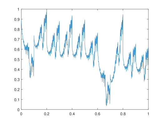
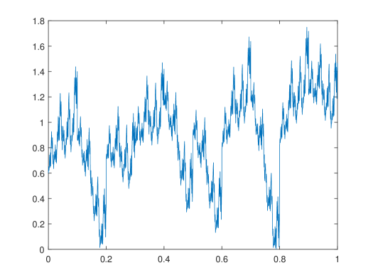
Figure 1.

Figure 2.

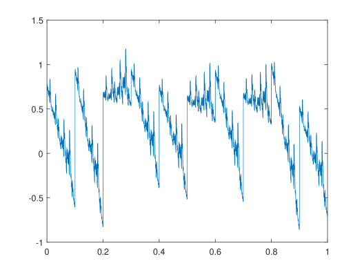
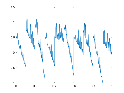
Figure 3.

Figure 4.

Here, we have the functional equation

$$F_{j}(x,y)=T(y)+q_{j}(x),~{}~{}j\in J,$$

and the self-referential equation is

$$f(L_{j}(x))=T(f(x))+q_{j}(x),x\in I_{j},j\in J.$$

We choose $q_{j}(x)=c_{j}x+d_{j}$ satisfying the join-up conditions such as

$$T(y_{1})+c_{j}x_{1}+d_{j}=y_{j}~{}\text{and}~{}T(y_{N})+c_{j}x_{N}+d_{j}=y_{j+1},~{}j\in J.$$

So, we have

$$c_{j}=\frac{(y_{j}-y_{j+1})-(T(y_{1})-T(y_{N}))}{(x_{1}-x_{N})}$$

and

$$d_{j}=y_{j}-T(y_{1})-\frac{(y_{j}-y_{j+1})-(T(y_{1})-T(y_{N}))}{(x_{1}-x_{N})}x_{1}.$$

The initial data is taken as follows for Figure 1 and Figure 2, respectively.
$\{(0,0.9),(0.1,0.5),(0.2,0.75),(0.3,0.95),(0.4,1.25),(0.5,1.5),(0.6,1.6),(0.7,1.2),\\ (0.8,1.8),(0.9,1.9),(1.0,2.0)\}$ and $\{(0,0.6),(0.1,1.4),(0.2,0.9),(0.3,1.2),(0.4,1.8),\\ (0.5,1.3),(0.6,0.9),(0.7,1.75),(0.8,0.85),(0.9,1.75),(1.0,2.0)\}.$
For Figure 3 and Figure 4, we consider $q_{j}(x)=x^{2}+c_{j}x+d_{j}$ satisfying the join-up conditions such as

$$T(y_{1})+x_{1}^{2}+c_{j}x_{1}+d_{j}=y_{j}~{}\text{and}~{}T(y_{N})+x_{n}^{2}+c_{j}x_{N}+d_{j}=y_{j+1},~{}j\in J.$$

So, we have

$$c_{j}=\frac{(y_{j}-y_{j+1})-(T(y_{1})-T(y_{N}))-(x_{1}^{2}-x_{N}^{2})}{(x_{1}-x_{N})}$$

and

$$d_{j}=y_{j}-T(y_{1})-\frac{(y_{j}-y_{j+1})-(T(y_{1})-T(y_{N}))-(x_{1}^{2}-x_{N}^{2})}{(x_{1}-x_{N})}x_{1}.$$

The initial data is taken as follows for Figure 3 and Figure 4, respectively.
$\{(0,0.75),(0.1,1.4),(0.2,0.65),(0.3,1.55),(0.4,1.25),(0.5,1.0),(0.6,1.75),(0.7,1.3),\\ (0.8,2.0),(0.9,1.15),(1.0,0.95)\}$ and $\{(0,0.5),(0.1,1.5),(0.2,1.75),(0.3,0.95),(0.4,1.0),\\ (0.5,1.8),(0.6,1.2),(0.7,1.6),(0.8,1.4),(0.9,0.85),(1.0,1.4)\}.$

Acknowledgements

The first author’s work is financially supported by the CSIR, India, with grant number 09/1058(0012)/2018-EMR-I.

References

- [1] G. Beer, Metric spaces on which continuous functions are uniformly continuous and Hausdorff distance, Proc. Amer. Math. Soc. 95 (1985) 653-658.
- [2] M. F. Barnsley, Fractal functions and interpolation, Constr. Approx. 2 (1986) 303-329.
- [3] M. F. Barnsley, Fractal Everywhere, Academic Press, Orlando, Florida, 1988. SIAM J. Math. Anal. 20(5) (1989) 1218–1242.
- [4] M. F. Barnsley and P. R. Massopust, Bilinear fractal interpolation and box dimension, J. Approx. Theory 192 (2015) 362–378.
- [5] Z. M. Balogh and J. T. Tyson, Hausdorff dimension of self-similar and self-affine fractals the Heisenberg group, Proc. London Math. Soc. (3) 91 (2005) 153-183.
- [6] D. Cheng, Z. Liand and B. Selmi, Upper metric mean dimensions with potential on subsets. Nonlinearity. 34 (2021) 852–867.
- [7] S. Chandra and S. Abbas, On fractal dimensions of fractal functions using functions spaces, Bull. Aust. Math. Soc. (2022) 1-11.
- [8] Van Dung, Nguyen and Adrian Petruşel, On iterated function systems consisting of Kannan maps, Reich maps, Chatterjea type maps, and related results, Journal of Fixed Point Theory and Applications 19, no. 4 (2017), 2271-2285.
- [9] J. E. Hutchinson, Fractals and self-similarity, Indian Univ. Math. J. 30 (1981) 713-747.
- [10] Janos Ludvik, On Mappings Contractive in the Sense of Kannan, Proceedings of the American Mathematical Society 61, no. 1 (1976): 171-75.
- [11] K. J. Falconer, Fractal Geometry: Mathematical Foundations and Applications, John Wiley Sons Inc., New York, 1999.
- [12] S. Jha and S. Verma, Dimensional analysis of -fractal functions, Results in Mathematics 76 (4) (2021) 1-24.
- [13] R. Kannan, Some results on fixed points, Bull. Calcutta Math. Soc. 60 (1968) 71-76.
- [14] R. Kannan, Some results on fixed points II, Amer. Math. Monthly 76 (1969) 405-408.
- [15] Y. S. Liang, Box dimensions of Riemann-Liouville fractional integrals of continuous functions of bounded variation, Nonlin. Anal. 72(11) (2010) 4304-4306.
- [16] P. R. Massopust, Fractal Functions, Fractal Surfaces, and Wavelets. 2nd ed., Academic Press, San Diego, 2016.
- [17] M. A. Navascués, Fractal polynomial interpolation, Z. Anal. Anwend. 25(2) (2005) 401-418.
- [18] M. A. Navascués, Fractal approximation, Complex Anal. Oper. Theory 4(4) (2010) 953-974.
- [19] A. Priyadarshi, Lower bound on the Hausdorf dimension of a set of complex continued fractions. J. Math. Anal. Appl. 449(1), (2017) 91–95.
- [20] S.I. Ri, A new idea to construct the fractal interpolation function, Indag. Math. 29(3) (2018) 962-971.
- [21] S.I. Ri, Fractal functions on the Sierpinski gasket, Chaos, Solitons Fractals 138 (2020) 110142.
- [22] H.J. Ruan, W.-Y. Sub and K. Yao, Box dimension and fractional integral of linear fractal interpolation functions, J. Approx. Theory 161 (2009) 187-197.
- [23] D. R. Sahu, A. Chakraborty and R. P. Dubey, K-Iterated function system, Fractals 18 (2010) 139–144.
- [24] B. Selmi, Multifractal dimensions for projections of measures. Bol. Soc. Paran. Mat. 40 (2022) 1-15.
- [25] B. Selmi, On the multifractal dimensions of product measures. Nonlinear Studies, 29(1) (2022).
- [26] R. D. Nussbaum, A. Priyadarshi and S. V. Lunel, Positive operators and Hausdorff dimension of invariant sets, Trans. Amer. Math. Soc. 364(2) (2012) 1029-1066.
- [27] H. Y. Wang and J. S. Yu, Fractal interpolation functions with variable parameters and their analytical properties, J. Approx. Theory 175 (2013) 1-18.