Characterizing Quantile-varying Covariate Effects under the Accelerated Failure Time Model

Abstract

An important task in survival analysis is choosing a structure for the relationship between covariates of interest and the time-to-event outcome. For example, the accelerated failure time (AFT) model structures each covariate effect as a constant multiplicative shift in the outcome distribution across all survival quantiles. Though parsimonious, this structure cannot detect or capture effects that differ across quantiles of the distribution, a limitation that is analogous to only permitting proportional hazards in the Cox model. To address this, we propose a general framework for quantile-varying multiplicative effects under the AFT model. Specifically, we embed flexible regression structures within the AFT model, and derive a novel formula for interpretable effects on the quantile scale. A regression standardization scheme based on the g-formula is proposed to enable estimation of both covariate-conditional and marginal effects for an exposure of interest. We implement a user-friendly Bayesian approach for estimation and quantification of uncertainty, while accounting for left truncation and complex censoring. We emphasize the intuitive interpretation of this model through numerical and graphical tools, and illustrate its performance by application to a study of Alzheimer’s disease and dementia.

Keywords: Accelerated failure time model; Bayesian survival analysis; Left-truncation; Time-varying coefficients; Time-varying covariates

This is the pre-peer reviewed, “submitted” version of the following article which is published in Biostatistics by Oxford University Press:

Reeder HT, Lee KH, Haneuse S. Characterizing quantile-varying covariate effects under the accelerated failure time model. Biostatistics. kxac052. 2022 Jan 04. doi: 10.1093/biostatistics/kxac052. PMID: 36610077.

Arxiv will be updated with the final peer-reviewed “accepted” version of the manuscript after a 24 month embargo period.

1 Introduction

Modeling the relationship between a time-to-event outcome $T$ and a vector of covariates $\mathbf{X}$ requires choosing a structure for the covariate effects. The proportional hazards model is by far the most commonly used model, specifying a constant multiplicative effect on the hazard of the outcome, yielding a ‘hazard ratio.’ Though ubiquitous, hazard ratios can be difficult to interpret, and the constant effect across time—that is, the ‘proportionality’ of the hazards—is not always plausible (Hernán,, 2010; Uno et al.,, 2015). As an alternative, the accelerated failure time (AFT) model directly describes shifts in the outcome distribution between populations having different characteristics, via multiplicative effects on event time quantiles (Wei,, 1992). Specifically, every survival quantile is multiplied by a constant ‘acceleration factor,’ equivalent to a horizontal stretching or compressing of the survivor function. In other words, the times by which 10 percent of events occur, or 90 percent, or 50 percent (i.e., the median survival time), or any other quantile, are shifted by the same multiplicative (or relative) constant. This common effect across quantiles is the central feature of the AFT model, making it highly interpretable because contrasts of survival quantiles are tangible and often clinically meaningful. Despite the parsimony of a constant multiplicative effect, in some settings it may be important to allow for more flexible effects across quantiles. For example, consider the study of Alzheimer’s disease (AD) and dementia among older adults. Prospective cohort studies of incident AD and dementia typically enroll subjects and follow them over decades, often subject to left truncation and sometimes complex censoring. Age at AD onset among those with a particular risk factor, for example, may skew earlier than among those without the risk factor. However, because AD is a complex disease that can arise over a long time scale, baseline risk factors may not affect the entire distribution uniformly. This could occur if, for example, a risk factor did not affect the timing of ‘early-onset’ cases, but made ‘late-onset’ cases occur sooner.

Modeling hazard ratios flexibly across time is a well-known and commonly used tool under the Cox model, but analogous extensions of the AFT model are not well-studied. Very recently, a paper by Crowther et al., (2022) suggests a frequentist spline-based AFT model and discusses potential for time-varying effects. However, their work considers a less common interpretation of the acceleration factor on the scale of log time, rather than investigating the potential for flexibility on the quantile scale. Moreover, their paper does not present any numerical results for the use of flexible effects. Separately, a recent paper by Pang et al., (2021) considers a Frequentist spline-based AFT model using a completely different formulation derived from Prentice and Kalbfleisch, (1979), requiring a specialized estimation algorithm and bootstrapping for inference. However, these papers do not incorporate left truncation or complex censoring, or consider effects of time-dependent covariates that commonly arise in longitudinal studies, for which the resulting relationship varies both over the trajectory of the covariate, and over the survival quantiles.

In this paper, we extend the AFT model to allow flexible acceleration factors that vary across quantiles, while simultaneously accommodating left-truncation, complex censoring, and time-varying covariates. Our approach builds on a time-varying AFT model first introduced in Cox and Oakes, (1984) but seemingly largely overlooked in the literature, and a general framework for flexible covariate effect specification. We illustrate how AFT regression coefficients specified to vary over time can be inverted into quantile-varying acceleration factors, and we develop a regression standardization scheme based on the g-formula to allow estimation of both covariate-conditional and marginal acceleration factors for an exposure of interest. We propose a Bayesian estimation approach for this modeling framework using the Stan language, which allows rigorous quantification of uncertainty and increased modeling flexibility. Through this investigation, we also uncover new insights into the use of binary time-varying covariates under the AFT model, and present novel tools for modeling and visualizing such effects. This further expands the AFT modeling toolkit to cover many extensions commonly used under the Cox model. We motivate these methods with an in-depth analysis of the Religious Orders Study and Memory and Aging Project prospective cohort studies of AD and dementia (Bennett et al.,, 2018).

2 The Accelerated Failure Time Model

The standard AFT model with time-invariant effects can be written as a log-linear model of time:

$$\log(T) =\mathbf{X}^{{\mathsf{\scriptscriptstyle T}}}\boldsymbol{\beta}+\epsilon,$$ (1)

where $\epsilon$ is a random error term and $\boldsymbol{\beta}$ is a vector of regression coefficients corresponding with covariates $\mathbf{X}$. We denote the exponentiated error $T_{0}=\exp(\epsilon)$, which represents a hypothetical random variable drawn from the “baseline distribution” having survivor function $S_{0}$. It is straightforward to show that this model structures covariate effects such that the distribution of event times among subjects having covariate pattern $\mathbf{x}$, denoted $T_{\mathbf{x}}$, is directly shifted from the baseline distribution by the transformation

$$T_{\mathbf{x}}\times\exp(-\mathbf{x}^{{\mathsf{\scriptscriptstyle T}}}\boldsymbol{\beta})\sim S_{0}.$$ (2)

Based on this connection, an equivalent representation of the standard AFT model is given directly via the baseline survivor function $S_{0}$ as

$$S(t\mid\mathbf{X}) =S_{0}(t\times\exp(-\mathbf{X}^{{\mathsf{\scriptscriptstyle T}}}\boldsymbol{\beta})).$$ (3)

The AFT model admits a direct interpretation of covariate effects as multiplicative shifts of the survival quantiles. For any particular quantile $p$, define $t_{\mathbf{x}}^{(p)}$ and $t_{0}^{(p)}$ to be the $p$th quantile times under $\mathbf{x}$ and baseline respectively. Then

$$p =S(t^{(p)}_{\mathbf{x}}\mid\mathbf{x})=S_{0}(t^{(p)}_{\mathbf{x}}\times\exp(-\mathbf{x}^{{\mathsf{\scriptscriptstyle T}}}\boldsymbol{\beta}))=S_{0}(t^{(p)}_{0}).$$ (4)

Solving for the $p$th quantile survival time under $\mathbf{x}$ yields

$$t^{(p)}_{\mathbf{x}}=S^{-1}(p\mid\mathbf{x})=S_{0}^{-1}(p)\exp(\mathbf{x}^{{\mathsf{\scriptscriptstyle T}}}\boldsymbol{\beta}).$$ (5)

The acceleration factor between two arbitrary covariate patterns $\mathbf{x}$ and $\mathbf{x}^{\prime}$ is then defined as the ratio of $p$th quantiles,

$$t^{(p)}_{\mathbf{x}}/t^{(p)}_{\mathbf{x}^{\prime}}=\frac{S_{0}^{-1}(p)\exp(\mathbf{x}^{{\mathsf{\scriptscriptstyle T}}}\boldsymbol{\beta})}{S_{0}^{-1}(p)\exp((\mathbf{x}^{\prime})^{{\mathsf{\scriptscriptstyle T}}}\boldsymbol{\beta})}=\exp((\mathbf{x}-\mathbf{x}^{\prime})^{{\mathsf{\scriptscriptstyle T}}}\boldsymbol{\beta}).$$ (6)

Under the standard AFT model, the acceleration factor does not depend on the form of $S_{0}$ or the value of $p$, and thus characterizes a constant multiplicative covariate effect across the entire distribution.

2.1 AFT model with time-varying components

In the standard AFT model (3), the covariate-adjusted survivor function is directly characterized by the time shift defined by $t\times\exp(-\mathbf{X}^{{\mathsf{\scriptscriptstyle T}}}\boldsymbol{\beta})$. Towards a more flexible AFT model, we replace this time shift with a general increasing function $V(t\mid\mathbf{X})$, yielding the covariate-adjusted survivor function

$$S(t\mid\mathbf{X}) =S_{0}\left(V(t\mid\mathbf{X})\right).$$ (7)

This formulation, first discussed by Cox and Oakes, (1984) in the context of time-varying covariates, reduces to the standard AFT when $V(t\mid\mathbf{X})=t\times\exp(-\mathbf{X}^{{\mathsf{\scriptscriptstyle T}}}\boldsymbol{\beta})$, while also admitting other temporal specifications of the relationship between covariates and the outcome distribution. In fact, one interpretation of this $V$ function is as a transformation linking the distribution of $T_{\mathbf{x}}$ under covariates $\mathbf{x}$, and the baseline distribution of $T_{0}$,

$$V(T_{\mathbf{x}}\mid\mathbf{x})\sim S_{0}.$$ (8)

Under this extended AFT model (7), the $p$th quantile survival time for subjects under covariate pattern $\mathbf{x}$ is

$$t^{(p)}_{\mathbf{x}} =S^{-1}(p\mid\mathbf{x})=V^{-1}(S_{0}^{-1}(p)\mid\mathbf{x}).$$ (9)

Now it may no longer be the case that the ratio of $p$th quantile survival times between covariate patterns $\mathbf{x}$ and $\mathbf{x}^{\prime}$ is a constant factor. Instead, the more general quantile-varying acceleration factor is

$$\xi(p\mid\mathbf{x},\mathbf{x}^{\prime},S_{0})=t^{(p)}_{\mathbf{x}}/t^{(p)}_{\mathbf{x}^{\prime}}=\frac{S^{-1}(p\mid\mathbf{x})}{S^{-1}(p\mid\mathbf{x}^{\prime})}=\frac{V^{-1}(S_{0}^{-1}(p)\mid\mathbf{x})}{V^{-1}(S_{0}^{-1}(p)\mid\mathbf{x}^{\prime})},$$ (10)

with notation explicitly capturing the additional potential for dependence on $p$ and $S_{0}$.

2.1.1 Examples and Interpretation

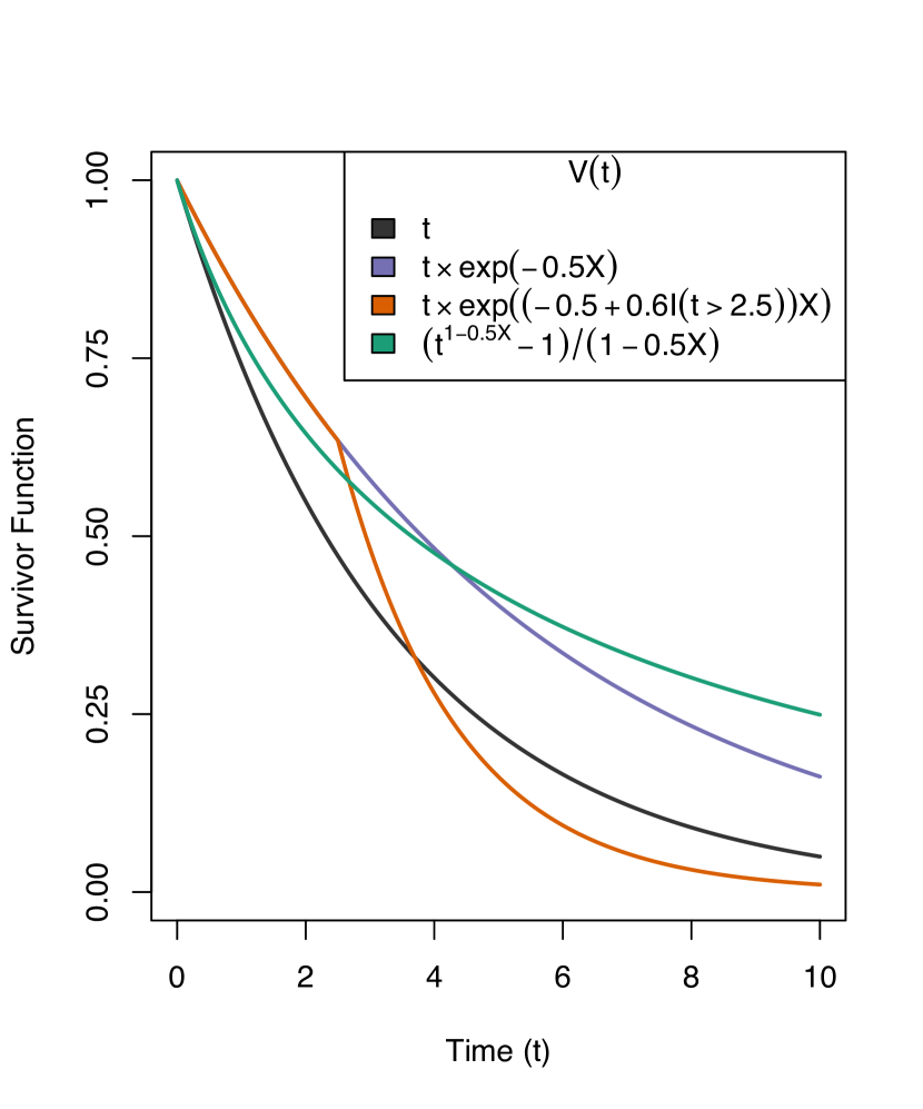
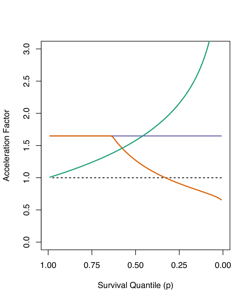
Figure 1: Sample survivor curves (left panel) and corresponding, possibly quantile-varying, acceleration factors (right panel). Baseline survivor function shown is $S_{0}(t)=\exp(-0.3t)$.

To emphasize both the flexibility and interpretability of this new quantity, Figure 1 shows sample survivor curves and corresponding acceleration factors under simple forms of quantile-varying effect for a single contrast between exposure levels $X=1$ and $X=0$, with baseline $S_{0}(t)=\exp(-0.3t)$. For simplicity we will interpret the effects at $p=0.75$ and $p=0.25$, which represent the time by which 25% and 75% of people experience the event, respectively.

As a reference point, the blue curve (second row of the legend) in each figure shows a constant acceleration factor of $\exp(0.5)\approx 1.65$, constant across quantiles. The green curve (fourth row of the legend) shows a protective effect that is increasingly pronounced among later-onset cases, with $\xi(0.75\mid 1,0)=1.25$ and $\xi(0.25\mid 1,0)=2$. In words, the estimated time by which 25% of the exposed die is 1.25 times as great as that among the unexposed, but the estimated time by which 75% of the exposed die is 2 times greater than unexposed. Conceptually, this form of protective effect corresponds with delayed onset of all cases among the exposed, but specifically a much longer tail of late-onset cases compared to a standard AFT protective effect.

The orange curve (third row of the legend) shows a more nuanced effect that delays the earliest cases, while also accelerating later onset cases. Numerically, $\xi(0.75\mid 1,0)=1.65$ and $\xi(0.25\mid 1,0)=0.9$, meaning the estimated time by which 25% of the exposed die is 1.65 times as great as that among the unexposed, but the estimated time by which 75% of the exposed die is only 0.9 times as great as among the unexposed. Conceptually, this form of effect is a ‘compressing’ of the outcome distribution, with earlier events being delayed and later events being accelerated. This is visible in the relative steepness of the survivor curve, with more than 50% of all events occurring between times 2 and 4. Furthermore, this represents an effect with ‘crossing survivor curves’, which despite being common in certain health research domains cannot be modeled by standard proportional hazards or AFT models. In summary, we see that this approach to conceptualizing covariate effects for time-to-event outcomes yields nuanced and interpretable insights beyond what is available from standard proportional hazards or AFT models.

3 Model Definition

The proposed quantile-varying AFT model is purposefully general with respect to the baseline survivor distribution $S_{0}$ and the time-varying covariate process $V$. In this section we outline several choices for specifying these model components, weighing tradeoffs between flexibility, stability, and computation. While this modeling framework in principle admits estimation under both frequentist and Bayesian paradigms, we focus on the latter approach and employ a Markov Chain Monte Carlo (MCMC) estimation routine via the No-U-Turn sampler implemented in the Stan language (Carpenter et al.,, 2017).

3.1 Specification of the covariate process $V$

For ease of exposition, we will consider a $d$ length vector of baseline covariates $\mathbf{X}$, of which an exposure of interest $X_{1}$ is specified with a flexible regression effect. However, this can easily be expanded to allow multiple such exposures of interest.

The form of the covariate process $V$ dictates the potential shapes the quantile-varying acceleration factor for $X_{1}$ can take, and requires a balance of flexibility and stability. We focus on spline-based methods, which require a vector of knots $\boldsymbol{\tau}$ characterizing a set of $J$ basis functions $B_{1},\dots,B_{J}$, and corresponding coefficients $\boldsymbol{\alpha}=(\alpha_{1},\dots,\alpha_{J})^{{\mathsf{\scriptscriptstyle T}}}$. This results in the specification

$$V(t\mid\mathbf{X})=t\times\exp\left(-\mathbf{X}^{{\mathsf{\scriptscriptstyle T}}}\boldsymbol{\beta}-X_{1}\sum_{j=1}^{J}\alpha_{j}B_{j}(t\mid\boldsymbol{\tau})\right),$$ (11)

Note that when $\boldsymbol{\alpha}={\mathbf{0}}$, then this reduces to the standard AFT model, allowing straightforward model comparison to assess the flexible effect specification. Furthermore, letting $B^{\prime}_{j}(t\mid\boldsymbol{\tau})=dB_{j}(t\mid\boldsymbol{\tau})/dt$, then the derivative of the covariate process, which is used in likelihood computation, has the simple form

$$v(t\mid\mathbf{X})=\frac{d}{dt}V(t\mid\boldsymbol{\tau})=V(t\mid\boldsymbol{\tau})\left[\frac{1}{t}-X_{1}\sum_{j=1}^{J}\alpha_{j}B^{\prime}_{j}(t\mid\boldsymbol{\tau})\right].$$ (12)

One specification inspired by the parametric proportional hazards spline model of Royston and Parmar, (2002) and discussed by Crowther et al., (2022) is the natural cubic spline basis, which combines cubic polynomial basis functions with a restriction that the ends beyond the lower and upper boundary knots be linear. Numerically stable forms for each natural cubic spline basis function $B_{k}$ and $B^{\prime}_{k}$ are readily available in statistical software, and the resulting $V$ combines flexibility and stability, with the added advantage of being a smooth function of time. However, the inverse $V^{-1}(t\mid\mathbf{X})$ used in the quantile-varying acceleration factor (10) does not have a closed form, and must be computed numerically.

A computationally simpler alternative is to specify $V$ as a piecewise linear function, which yields a simplified analytical form and closed form inverse. Define $J+2$ knots $0=\tau_{0}<\tau_{1}<\dots<\tau_{J}<\tau_{J+1}=\infty$, with basis functions defined $B_{j}(t\mid\boldsymbol{\tau})=t^{-1}(\min\{t,\tau_{j+1}\}-\tau_{j})_{+}$ where $(z)_{+}=\min\{0,z\}$. Then the final specification for $V$ simplifies to

$$V(t\mid\mathbf{X})=t\times\exp\left(-\mathbf{X}^{{\mathsf{\scriptscriptstyle T}}}\boldsymbol{\beta}\right)\left[\sum_{j=1}^{J}\exp\left(-X_{1}\alpha_{j}\right)B_{j}(t\mid\boldsymbol{\tau})\right],$$ (13)

with the straightforward derivative $v(t\mid\mathbf{X})=\exp\left\{-\mathbf{X}^{{\mathsf{\scriptscriptstyle T}}}\boldsymbol{\beta}-\sum_{j=1}^{J}X_{1}\alpha_{j}\mathbb{I}(\tau_{j}\leq t<\tau_{j+1})\right\}$. Computation of the inverse is also straightward, and left to Appendix B of the Supplementary Materials. As above, this reduces to the standard AFT model when $\boldsymbol{\alpha}={\mathbf{0}}$.

3.2 Specification of the baseline distribution $S_{0}$

As with the specification of $V$, there are numerous possible choices of baseline distribution characterizing $S_{0}$, both fully parametric and semi-parametric. Parametric specifications have several advantages in this setting: they are computationally efficient, well-defined across all quantiles, have tractible inverse survivor functions, and can lead to improved efficiency in smaller samples. Two such parametric specifications are the log-Normal baseline distribution with survivor function defined by $S_{0}(t\mid\mu,\sigma)=1-\Phi(\log t-\mu)/\sigma^{2}$ where $\Phi(\cdot)$ is the standard normal distribution function, and the Weibull baseline distribution defined by $S_{0}(t\mid\mu,\sigma)=\exp\left\{\left[t\times\exp(-\mu)\right]^{\sigma}\right\}$. Let $\boldsymbol{\phi}=(\mu,\sigma)^{{\mathsf{\scriptscriptstyle T}}}$ denote the collection of parameters corresponding to the baseline distribution.

Nevertheless, an important benefit of the Bayesian paradigm is the well-established literature on semi-parametric AFT survival models with flexible baseline distributions, such as Dirichlet process mixture (DPM) models (Lee et al.,, 2017) and Polya tree priors (Hanson et al.,, 2009). Here we propose a transformed Bernstein polynomial (TBP) prior for $S_{0}$ following (Zhou and Hanson,, 2018), which defines a parametric centering distribution having survivor function $S^{*}_{0}(t\mid\boldsymbol{\phi})$ (such as the Weibull or log-Normal defined above), then applies a transformation using Bernstein polynomial functions to can flexibly capture a wide array of distributions. Formally, define the Beta($a,b$) distribution function

$$G(p\mid a,b)=\frac{\Gamma(a+b)}{\Gamma(a)\Gamma(b)}p^{a-1}(1-p)^{b-1},\quad 0\leq x\leq 1,$$

and a vector $\mathbf{w}$ of length $K$ such that $\sum_{k=1}^{K}w_{k}=1$. Then the baseline survivor function is the linear combination

$$S_{0}(t\mid\boldsymbol{\phi},\mathbf{w})=\sum_{k=1}^{K}w_{k}G(S^{*}_{0}(t\mid\boldsymbol{\phi})\mid k,K-k+1).$$

Because the domain of $G$ and the range of $S^{*}_{0}$ are both [0,1], this represents a flexible spline transformation of the centering parametric distribution on the scale of survival quantiles. In particular, if $\mathbf{w}=(J^{-1},J^{-1},\dots,J^{-1})^{{\mathsf{\scriptscriptstyle T}}}$, then $S_{0}=S^{*}_{0}$, so the TBP specification contains the centering parametric model, but can also characterize a wide array of survival distribution shapes. An illustration is provided in Appendix D of the Supplementary Materials. To complete the Bayesian specification, we place a $\text{Dirichlet}(\theta)$ prior on $\mathbf{w}$ with $\theta>0$, where larger values of $\theta$ correspond to tighter concentration of the elements of $\mathbf{w}$ around $J^{-1}$ and therefore tighter concentration of $S_{0}$ around $S^{*}_{0}$.

This specification offers several advantages over other flexible baseline specifications mentioned previously. Importantly, each $G$ function can be computed recursively, so overall computation of $S_{0}$ is efficient. Moreover, the TBP prior can be straightforwardly sampled using the No-U-Turn algorithm implemented in the Stan language, as described below. By contrast, many other Bayesian non-parametric specifications such as Polya trees and DPM models require specialized computational methods such as custom MCMC samplers and data augmentation (Hanson et al.,, 2009; Lee et al.,, 2017). The main tradeoff with any flexible form for $S_{0}$ compared to a fully parametric specification is the increased computational cost, both for the sampler as well as the numerical computation of the inverse function $S^{-1}_{0}$ and associated acceleration factors.

3.3 Likelihood

Another important benefit of the Bayesian approach is the ability to seamlessly handle arbitrary censoring and left truncation. Let $(Y^{l},Y^{u})$ the left and right observed endpoints of a censoring interval around a true event time $T$, such that $Y^{l}\leq T\leq Y^{u}$. Right-censoring simply corresponds with $Y^{u}=\infty$. Define the binary indicator $\Delta=\mathbb{I}(Y^{l}=Y^{u})$ to be a subject observed to experience the event exactly at time $Y^{l}$. Finally, let $L$ represent the possible left-truncation time. Along with the baseline covariates $\mathbf{X}$, denote the corresponding observed data for the $i$th subject ${\mathcal{D}}_{i}=\{y_{i}^{l},y_{i}^{u},\delta_{i},l_{i},\mathbf{x}_{i}\}$.

After specifying $V$ and $S_{0}$, let $\boldsymbol{\psi}=(\boldsymbol{\beta}^{{\mathsf{\scriptscriptstyle T}}},\boldsymbol{\alpha}^{{\mathsf{\scriptscriptstyle T}}},\boldsymbol{\phi}^{{\mathsf{\scriptscriptstyle T}}},\mathbf{w}^{{\mathsf{\scriptscriptstyle T}}})^{{\mathsf{\scriptscriptstyle T}}}$ denote the full set of parameters. Then assuming that censoring is non-informative of the outcome, the resulting likelihood contribution for subject $i$ is then

$${\mathcal{L}}_{i}(\boldsymbol{\psi}\mid{\mathcal{D}}_{i})=\frac{[f_{0}(V(y_{i}^{l}\mid\mathbf{x}_{i}))v(y_{i}^{l}\mid\mathbf{x}_{i})]^{\delta_{i}}[S_{0}(V(y_{i}^{l}\mid\mathbf{x}_{i}))-S_{0}(V(y_{i}^{u}\mid\mathbf{x}_{i}))]^{(1-\delta_{i})}}{S_{0}(V(l_{i}\mid\mathbf{x}_{i}))}$$ (14)

where $f_{0}$ is the density function corresponding to the baseline distribution. By convention, $S_{0}(\infty)=0$, so under right-censoring this reduces to the standard censored data likelihood.

3.4 Bayesian Computation and Prior Specification

To implement this modeling framework, we propose Bayesian estimation via the No-U-Turn sampler implemented by the Stan language (Carpenter et al.,, 2017). In brief, this MCMC algorithm uses gradient information on the log-posterior to generate Markov transitions that efficiently explore the posterior distribution. This choice reflects our goal of developing a practical and accessible methodology, as our implementation can be easily called from R via the rstan package with minimal algorithmic tuning (Stan Development Team,, 2020).

To complete our model specification, we consider priors on the parameters $\boldsymbol{\beta}$, $\boldsymbol{\alpha}$, and $\boldsymbol{\phi}$. The No-U-Turn sampler does not require or leverage conjugacy between prior and posterior, so prior distributions can be chosen or adjusted without changing the implementation of the sampler. In the application below, we adopt flat priors for regression parameters $\boldsymbol{\beta}$ and $\boldsymbol{\alpha}$. For the parametric (centering) distribution, we also adopt a flat prior for the log location parameter $\log\mu$, and for the scale parameter a $\sigma\sim\text{Gamma}(a_{\sigma},b_{\sigma})$ prior. The TBP prior is defined by a $\mathbf{w}\sim\text{Dirichlet}(\theta)$ prior for the weights, and we adopt a $\theta\sim\text{Gamma}(a_{\theta},b_{\theta})$ hyperprior on $\theta$, regulating the level of flexibility around the parametric centering distribution.

3.5 Model Evaluation and Comparison

A conceptual benefit of our proposed modeling framework is that the flexible structures naturally encompass simpler models: the standard AFT model is nested within the flexible effect specification of covariate process $V$, and a fully parametric baseline is nested within the TBP prior for $S_{0}$. In this section, we propose a model evaluation metric to inform decisions regarding the necessary level of model complexity, facilitated by the Stan language and the loo package in R (Vehtari et al.,, 2017).

The expected log pointwise predictive density (ELPD) is a metric that evaluates how well a fitted model can predict future out-of-sample data, with larger values indicating better predictive ability. For $n$ future observations ${\widetilde{y}}_{1},\dots,{\widetilde{y}}_{n}$, the ELPD is defined via the posterior predictive density $p({\widetilde{y}}\mid{\mathcal{D}})$ as

$$\text{ELPD}=\sum_{i=1}^{n}\int\log p({\widetilde{y}}_{i}\mid{\mathcal{D}})d{\widetilde{y}}_{i}.$$ (15)

While typically future out-of-sample data is not available, the ELPD can be estimated by leave-one-out cross validation by averaging the log posterior predictive distribution for each observed data point of a model fit excluding that data point. This quantity can in turn be estimated efficiently from a single Bayesian model fit via Pareto smoothed importance sampling, which we denote $\widehat{\text{ELPD}}_{\text{psis-loo}}$ (Vehtari et al.,, 2017), and has been shown to exhibit improved performance relative to other common Bayesian model criteria, such as Deviance Information Criterion (DIC).

3.6 Computation of Regression Standardized Acceleration Factors

Importantly, under the covariate process $V$ defined by (11), the quantile-varying acceleration factor (10) depends on the specified values of all covariates $\mathbf{x}$ and $\mathbf{x}^{\prime}$, not just those that differ. This conditionality on the values of all covariates may be insightful if interest is in assessing effect heterogeneity in particular subpopulations defined by specific covariate patterns. However, practical interest is often in assessing the effect of an exposure in a population standardized with respect to the other covariates. Therefore, in this section we propose a regression standardization approach to estimating the quantile-varying acceleration factor for a particular covariate of interest, averaged over the distribution of other covariates. Conceptually, the goal is to first estimate the survivor curves we would observe in the population if everyone was alternately exposed or unexposed, and then back out the quantile-varying acceleration factor that relates the two curves.

For clarity, consider a single binary exposure of interest $X$, and vector of additional covariates $\mathbf{Z}$. Then the marginal ratio of interest is

$$\xi(p\mid X=1,X^{\prime}=0)=\frac{S^{-1}(p\mid X=1)}{S^{-1}(p\mid X=0)}.$$ (16)

Following Rothman et al., (2021) and Sjölander, (2016), define the survivor function for $X=x$, standardized to the distribution of $\mathbf{Z}$, as

$$S_{\mathbf{Z}}(t\mid x)=E_{\mathbf{Z}}[P(T>t\mid X=x,\mathbf{Z})].$$ (17)

Using standardized survivor functions, we define the standardized quantile-varying acceleration factor as

$$\xi_{\mathbf{Z}}(p\mid X=1,X^{\prime}=0)=\frac{[S_{\mathbf{Z}}]^{-1}(p\mid X=1)}{[S_{\mathbf{Z}}]^{-1}(p\mid X=0)}.$$ (18)

where $[S_{\mathbf{Z}}]^{-1}(p\mid X=x)$ is the function solving $S_{\mathbf{Z}}(t\mid X=x)-p=0$ for $t$. This contrast represents the magnitude of the horizontal shift in the standardized survivor curve $S_{\mathbf{Z}}$ between $X=1$ and $X=0$, at each quantile $p$.

To estimate and quantify uncertainty for these contrasts, we develop a novel approach based on the Bayesian g-formula (Keil et al.,, 2018). In brief, for each MCMC draw $m=1,\dots,M$, for each $X=x$ we compute the standardized survivor function

$$S^{(m)}_{\mathbf{Z}}(t\mid X=x)=n^{-1}\sum_{i=1}^{n}S(t\mid X=x,\mathbf{Z}=\mathbf{z}_{i};\boldsymbol{\psi}^{(m)}),$$ (19)

and then form contrast of interest

$$\xi^{(m)}_{\mathbf{Z}}(p\mid X=1,X^{\prime}=0)=\frac{[S^{(m)}_{\mathbf{Z}}]^{-1}(p\mid X=1)}{[S^{(m)}_{\mathbf{Z}}]^{-1}(p\mid X=0)}.$$ (20)

This may require numerical evaluation of the inverse standardized survivor functions. Estimating the posterior mean and credible intervals of $\xi_{\mathbf{Z}}$ proceeds using the mean and suitable quantiles of $\xi^{(1)}_{\mathbf{Z}},\dots,\xi^{(M)}_{\mathbf{Z}}$.

4 Application: Cohort Study of Incident AD and Dementia

Motivating the proposed AFT model is the study of adverse cognitive outcomes among older adults, for which long timescales and complex disease etiology naturally lend themselves to consideration of flexible covariate effects on the quantile scale. In this section we investigate risk factors for AD and dementia in older adults using data collected by the Religious Orders Study and Memory and Aging Project (ROSMAP) prospective cohort studies ongoing since 1994 and 1997 respectively (Bennett et al.,, 2018). Our analysis focuses on flexible estimation of the association of the genetic marker APOE-$\epsilon 4$ with the timing of AD or dementia onset. Previous analyses of similar cohorts have simply compared incidence rates within age categories to examine whether this marker had differential effects through time (Kukull et al.,, 2002). So, estimating a quantile-varying acceleration factor for APOE-$\epsilon 4$ is of clinical relevance, while also accounting for other risk factors.

2694 subjects were enrolled without AD or dementia between ages 65 and 86, and followed until withdrawal or death. Subjects underwent cognitive screening annually to diagnose onset of AD or dementia, and death status was monitored continuously. Table 1 summarizes a set of baseline binary risk factors collected on the subjects: marital status at baseline, sex, education level, race/ethnicity, and presence of the APOE-$\epsilon 4$ genetic variant. The final analysis dataset includes 2335 subjects with complete baseline information. The outcome is defined by the time of diagnosis of AD or dementia, with death treated as a censoring mechanism, yielding a cause-specific analysis. Because we only include subjects with age at least 65, the time scale of analysis is “years since age 65.” Importantly, our analysis accounts for the presence of left truncation (or “delayed entry”) by subjects who enroll after age 65. Though this framework admits interval censoring, given the short visit intervals relative to the timescale, for this analysis we defined the timing of AD onset at the midpoint of the corresponding visit interval.

We compare the fits of standard AFT models with those having piecewise and spline forms for $V$, under Weibull and log-Normal baseline specifications as well as a TBP prior baseline with $K=5$, centering around the Weibull distribution. We set 4 break points for the piecewise linear effect at 7.5 year intervals across the follow up period, and for the spline effect we set 2 internal knots at quantiles on the log scale. The difference between these specifications is due to the spline being naturally more flexible, allowing it to smooth across knots with irregular spacing, while the piecewise linear model requires break points that span the entire timespan in order to achieve flexibility. For the scale parameter we set the prior $\sigma\sim\text{Gamma}(0.3,0.05)$, having prior median 1.46 and 95% central mass between 6e-5 and 38. Finally, we fit a standard Frequentist Cox proportional hazards model for comparison. For the TBP concentration parameter we set a hyperprior of $\theta\sim\text{Gamma}(1,1)$. For each model we ran three chains each for 2000 adaptation iterations and 10000 samples, totalling 30000 samples. After sampling, all potential scale reduction factors were below $1.01$ and trace plots indicated good mixing.

Table 3 reports the estimates of regression parameters across all AFT specifications, as well as frequentist results from a Cox proportional hazards model. For the AFT models, positive estimates of $\boldsymbol{\beta}$ correspond with delayed onset of AD or dementia, as do negative estimates for the Cox model. The coefficients estimated for white race/ethnicity, marital status, female sex, and education are stable across all model specifications. Interpreting the Weibull AFT with constant effect of APOE-$\epsilon 4$, for example, indicates that being married is associated with a $\exp(0.09)=1.09$ times greater median time to onset of AD or dementia, with 95% credible interval of (1.02,1.19). Flexible effect coefficients of APOE-$\epsilon 4$ cannot be directly interpreted on the quantile scale, therefore we present graphical tools below.

The top panel of Table 2 compares estimates of ELPD model criterion for each AFT model. In each case, the spline and piecewise-linear effect specifications outperformed the standard AFT specification. The log-Normal models uniformly underperformed, while the Weibull and TBP models performed comparably. To graphically assess the effect of APOE-$\epsilon 4$ we report the TBP model, and present results for other specifications in Appendix A of the Supplementary Materials. Results were qualitatively similar for all baseline distributions, with the largest differences in acceleration factor only occurring in the lowest quantiles extrapolated beyond the observed data.

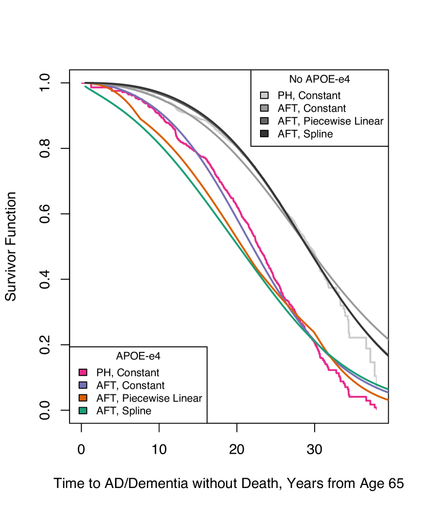
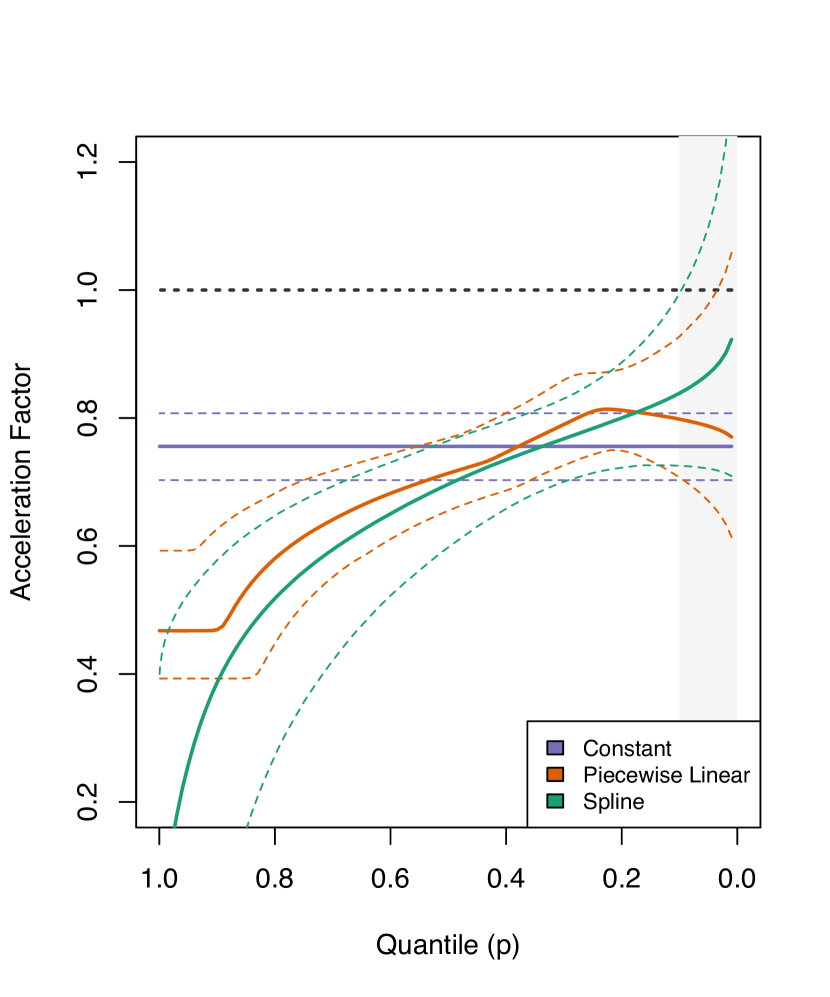
Figure 2: Under a Weibull-centered TBP baseline specification: (left panel) regression standardized survivor function estimates for onset of AD or dementia without death, averaged over other covariates. Regression standardized estimate from Cox proportional hazards model shown for comparison; (right panel) regression standardized quantile-varying acceleration factor estimates for onset of AD or dementia without death, averaged over other covariates. 95% credible intervals represented with dashed lines. Grey shaded region represents area of parametric extrapolation beyond quantiles observed in both groups.

Figure 2 shows the estimated survivor functions and corresponding quantile-varying acceleration factors for the APOE-$\epsilon 4$ genetic variant, after regression standardization over the distribution of the other baseline covariates. These figures confirm other findings that APOE-$\epsilon 4$ is associated with earlier onset of AD and dementia. However, quantile-varying effects also indicate that the acceleration is strongest among the earliest cases and subsequently diminishes. Both piecewise and spline models estimate that the time by which the first 10% of those living with APOE-$\epsilon 4$ develop AD or dementia is earlier than those without the variant by a factor of about 0.5; the median times by which people develop AD or dementia differ by a factor of about 0.75, and the times by which 75% develop AD or dementia differ by a factor of about 0.85. Due to censoring of those with advanced age, the acceleration factor at lower quantiles reflects parametric extrapolation beyond the observed distribution, represented in the figure by grey shading. Nevertheless, this finding has clear clinical significance, indicating the particular need to monitor for early onset AD at younger ages among those with APOE-$\epsilon 4$.

5 Effects of Time-varying Covariates on the Quantile Scale

In this section, we extend the proposed AFT model to incorporate binary time-varying covariates, and provide intuition and graphical tools for effectively interpreting and communicating corresponding effects on the quantile scale.

To focus on intuition, consider a single time-varying covariate denoted $X_{1}(t)$ with constant regression effect $\beta_{1}$. In particular, let $X_{1}(t)$ be a binary-valued step function, such as an indicator for whether a non-terminal event has occurred by time $t$. Formally, define $X_{1}(t)=\mathbb{I}(t>t_{X})$, where $t_{X}$ is the time at which $X_{1}$ changes. To simplify notation, consider a single additional covariate time-invariant covariate $X_{2}$, though inclusion of multiple additional covariates is straightforward. Embedding these covariates directly in the structure for $V$ given by (11) and setting $\boldsymbol{\alpha}={\mathbf{0}}$ to denote a constant effect yields

$$V(t\mid\mathbf{X}(t)) =t\times\exp\left(-X_{1}(t)\beta_{1}-X_{2}\beta_{2}\right)$$ (21)

$$=\exp\left(-X_{2}\beta_{2}\right)\left[\min\{t,t_{X}\}+(t-t_{X})_{+}\exp\left(-\beta_{1}\right)\right].$$

With complete derivation given in Appendix C of the Supplementary Materials, the acceleration factor at quantile $p$ between two subjects depends on each person’s value of $X_{2}$, the change time $t_{X}$ for $X_{1}$, and the baseline distribution $S_{0}$. In particular, for those with $X_{2}=x_{2}$, the acceleration factor at quantile $p$ for experiencing $X_{1}$ at $t_{X}$ versus not experiencing $X_{1}$ is

$$\frac{t_{X}}{S_{0}^{-1}(p)\exp(x_{2}\beta_{2})}+\exp(\beta_{1})\left[1-\frac{t_{X}}{S_{0}^{-1}(p)\exp(x_{2}\beta_{2})}\right].$$ (22)

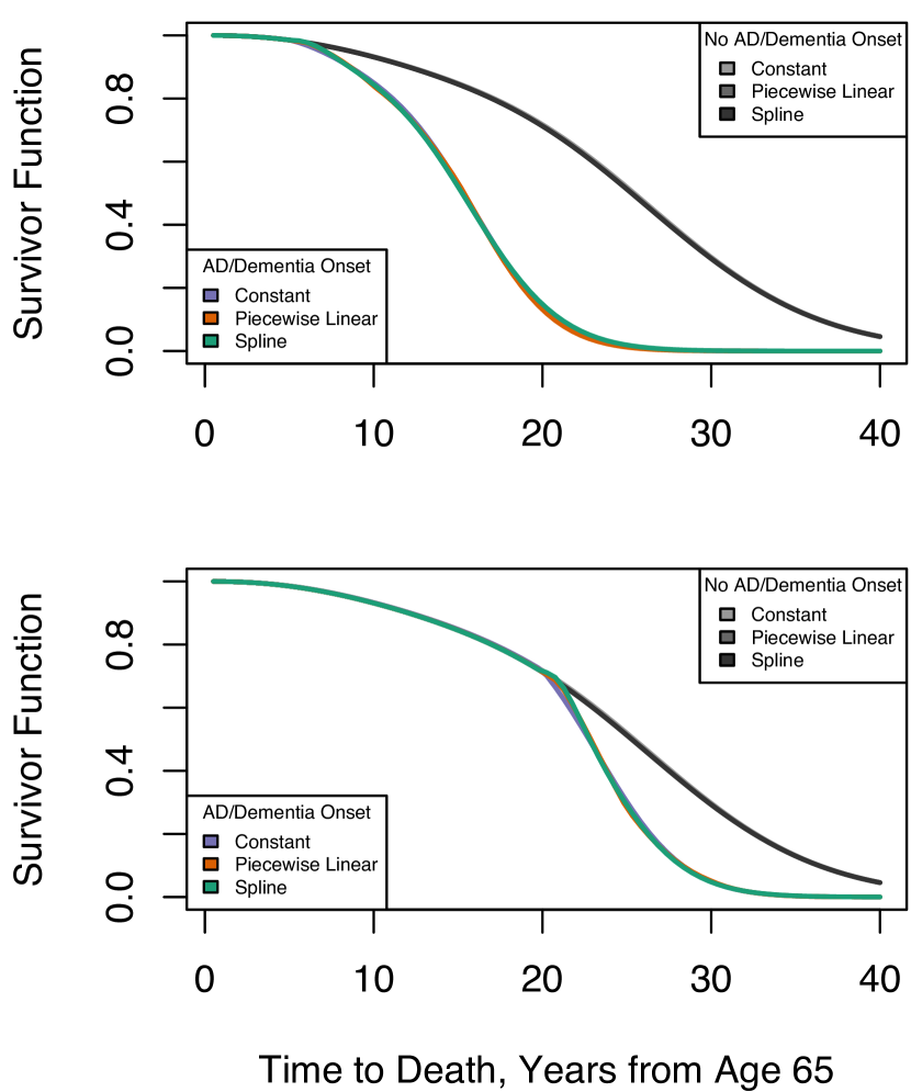
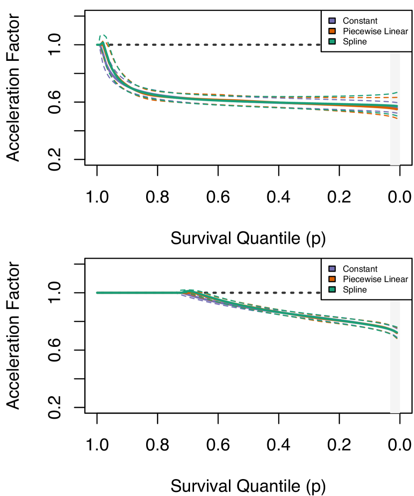
Figure 3: Under a Weibull-centered TBP baseline specification: (left panel) regression standardized survivor function estimates for mortality following onset of AD or dementia, averaged over other covariates; (Right panel) regression standardized survivor function estimates for mortality following onset of AD or dementia, averaged over other covariates. 95% credible intervals represented with dashed lines. Grey shaded region represents area of parametric extrapolation beyond quantiles observed in both groups.

This is a weighted average between 1 and $\exp(\beta_{1})$, with weight inversely proportional to the duration from $t_{X}$ to the $p$th quantile survival time in the comparison group, $S_{0}^{-1}(p)\exp(x_{2}\beta_{2})$. Intuitively, before $t_{X}$ there is no difference between the individuals, so the acceleration factor is 1, and then after $t_{X}$ the effect of $X_{1}$ starts accumulating, and the acceleration factor gradually shifts towards $\exp(\beta_{1})$, becoming more pronounced as $p$ extends towards 0. This dynamic is illustrated by example in Figure 3 below.

Finally, a flexible effect for $X_{1}(t)$ can also be specified by adapting the form of (21), yielding

$$V(t\mid\mathbf{X}(t))=e^{-X_{2}\beta_{2}}\left[\min\{t,t_{X}\}+(t-t_{X})_{+}\exp\left(-\beta_{1}-\sum_{k=1}^{K}\alpha_{k}B_{k}(t-t_{X}\mid\boldsymbol{\tau})\right)\right].$$ (23)

Following Haneuse et al., (2008), this specification characterizes flexibility in the effect of $X_{1}$ over the time scale $t-t_{X}$ denoting time since the non-terminal event, rather than on the overall time scale of $t$, enabling evaluation of the temporal effect of $X_{1}$ on its own timescale. Practically, this means that basis functions and knots $\boldsymbol{\tau}$ must be specified on the corresponding time scale.

5.1 Effect of Incident AD and Dementia on Mortality

To illustrate the use of the AFT framework with a time-varying binary covariate, we perform a secondary analysis of the cohort study to evaluate the association between onset of AD/dementia and subsequent time to death. We fit models specifying onset of AD/dementia as a binary time-varying covariate, adjusting for the same time-invariant baseline covariates as in the above analysis (including a constant effect for APOE-$\epsilon$4).

For the piecewise linear effect, we set break points at 1, 2, 3, 5, and 10 years after time of AD onset, and for the spline effect we set 2 internal knots at observed quantiles of time from AD onset to death on the log scale. Other settings and the sampling setup were as above, though for computation of the acceleration surface described below, we thinned the samples by a factor of 10 to facilitate computation. Table A.1 in Appendix A of the Supplementary Materials reports estimated model parameters varying baseline survival distribution and effect specification, along with frequentist results from an extended Cox proportional hazards model with AD/dementia onset as a time-varying covariate. As before, the coefficients estimated for all baseline covariates are stable across specifications for the flexible effect.

The lefthand panels of Figure 3 show estimated regression standardized survivor curves comparing those without AD/dementia onset, and and those with onset at age 70 and 85, respectively, under the TBP prior baseline specification. In each case, the curves are identical up until the time of onset, and then once AD/dementia onset occurs mortality increases substantially. The plots indicate similarity between models fit with piecewise and spline effects of AD/dementia onset relative to a constant effect, though the flexible models indicate a small delay in the mortality increase from the time of AD/dementia onset. The corresponding acceleration factors are given on the righthand panels of Figure 3, illustrating the trajectory derived in (22), where no association exists before the quantile of AD/dementia onset, followed by an increasingly pronounced association after AD/dementia onset.

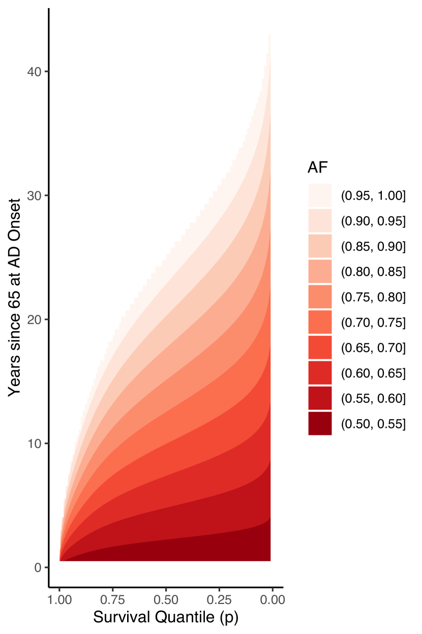
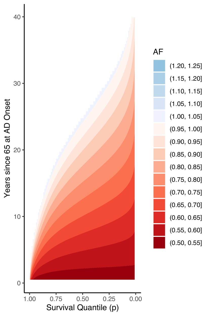
Figure 4: Under a Weibull-centered TBP baseline specification, contour plots of regression standardized acceleration factor surface estimates for death following onset of AD/dementia, standardized to other covariates. Time of AD/dementia onset is shown on y-axis, and subsequent survival quantile is shown on x-axis. Color indicates acceleration factor at the given survival quantile, comparing those with AD/dementia onset at the specified time and those without AD/dementia. Horizontal cross-sections illustrate quantile-varying acceleration factor for AD/dementia onset at a particular time, while vertical cross-sections illustrate acceleration factor at a particular quantile across times of AD/dementia onset. (Left panel) constant effect specification; (center panel) piecewise linear effect specification; (right panel) spline effect specification.

Selecting and plotting acceleration factors for a few AD/dementia onset times of interest may be sufficient in some settings, but fully communicating the results requires visualizing the quantile-varying effect across the entire range of the time-varying covariate. Figure 4 reports this acceleration factor surface as a contour plot, with the time of AD/dementia onset on the y-axis, the survival quantile on the x-axis, and the color representing the magnitude of the acceleration factor. The two acceleration factor plots in Figure 3 correspond with cross-sections of this surface, by drawing horizontal lines at times 5 and 20 on the y-axis. More generally, looking horizontally across this plot shows the quantile varying acceleration factor corresponding with different times of AD/dementia onset. However, this plot can also be read vertically, to show how the acceleration factor for a particular quantile changes depending on the timing of the time-varying covariate. For example, drawing a vertical line from 0.5 on the x-axis shows the acceleration factor for median survival, varying across times of AD/dementia onset. Therefore, this single plot allows us to read off complex regression effects both as a function of the survival quantile, as well as of the timing of the time-varying covariate.

6 Discussion

The AFT model’s specification of multiplicative covariate effects on the quantile scale provides an interpretable and attractive alternative to the standard proportional hazards model. Our proposed extensions to the AFT model enabling quantile-varying acceleration factors, and admitting binary time-varying covariates represent important additions to the standard toolbox for survival analysis. Just as the Cox proportional hazards model benefits from straightforward incorporation of time-varying hazard ratios, the ability to add flexibility to the AFT model regression effects expands the scope of scientific inquiry. Motivated by the study of AD in older adults, we found that the association of the APOE-$\epsilon 4$ gene with AD onset varied substantially across quantiles, with earlier-onset cases accelerated the most and later-onset cases the least.

Moreover, the ability to model, summarize, and communicate the effects of binary time-varying covariates creates new opportunities to capture nuanced associations between longitudinal health trajectories. Our proposed visualization of these effects as a surface across both the covariate timescale and the survival quantiles is particularly valuable, as previous work to incorporate time-varying covariates into AFT models has not focused on communication of effects of time-varying components on the quantile scale (Hanson et al.,, 2009; Zhou and Hanson,, 2018). In our application, this approach illustrated that the association between AD/dementia onset and subsequent mortality varies substantially both across survival quantiles, and depending on the time of AD/dementia onset.

Estimation within the Bayesian paradigm also contributes important benefits for our proposed methodology. In particular, the Bayesian paradigm enables flexible estimation of the baseline distribution using the TBP prior, and allows for seamless uncertainty quantification even after regression standardization (Keil et al.,, 2018). To our knowledge, ours is the first implementation of the TBP prior in Stan, and software in R is available at https://github.com/harrisonreeder/aftquantile.

Finally, this work complements the related literature on censored quantile regression (Portnoy,, 2003; Reich and Smith,, 2013). Censored quantile regression specifies an additive model for the effects of covariates on the quantile scale, while our model specifies multiplicative effects on the quantile scale. The biological plausibility or clinical relevance of additive versus multiplicative changes to the survival quantiles depends on the application, so our proposed methodology yields a valuable alternative to available quantile-based methods.

Funding

This project was supported by the Eunice Kennedy Shriver National Institute of Child Health and Human Development [grant number F31HD102159 to HTR]. The National Institutes on Aging supported the Religious Orders Study [grant numbers P30AG010161 and R01AG015819] and the Rush Memory and Aging Project [grant number R01AG017917].

Table 1: Baseline covariates by observed AD/dementia and death outcome status. All covariates are binary, with 1 indicating the presence of the status and 0 indicating absence.

		Censored prior	AD/dementia	Death	AD/dementia
		to AD/dementia	and censored	without	diagnosis
	Total (%)	or death (%)	prior to death (%)	AD/dementia (%)	and death (%)
Total	2335 (100%)	750 (100%)	123 (100%)	891 (100%)	571 (100%)
White Race/Ethnicity	2178 (93.3%)	687 (91.6%)	100 (81.3%)	849 (95.3%)	542 (94.9%)
Male Sex	648 (27.8%)	147 (19.6%)	24 (19.5%)	316 (35.5%)	161 (28.2%)
Married at Study Entry	462 (19.8%)	216 (28.8%)	29 (23.6%)	145 (16.3%)	72 (12.6%)
15+ Years of Education	1621 (69.4%)	532 (70.9%)	80 (65%)	609 (68.4%)	400 (70.1%)
APOE-$\epsilon 4$ Genetic Variant	575 (24.6%)	156 (20.8%)	53 (43.1%)	173 (19.4%)	193 (33.8%)

Table 2: Estimated expected log predictive density (ELPD), multiplied by -2 to replicate scale of information criteria. Smaller values indicate better model fit.

	AFT Model
	log-Normal	Weibull	TBP (Weibull Centered)
AD/Dementia Onset (Death as a Censoring Mechanism)
Constant	5862.0	5806.3	5804.4
Piecewise Linear	5841.5	5788.4	5786.5
Restricted Cubic Spline	5814.9	5780.9	5781.4
Death (AD/Dementia as a Time-Varying Covariate)
Constant	9997.2	9666.7	9628.2
Piecewise Linear	9919.8	9636.7	9600.1
Restricted Cubic Spline	9884.5	9600.9	9564.9

Table 3: Regression estimates for time to onset of AD or dementia in the absence of death. AFT results are posterior medians and 95% credible intervals for regression parameters. Cox model results are log-hazard ratio estimates and 95% confidence intervals.

		AFT Model
	Cox PH	log-Normal	Weibull	TBP (Weibull Centered)
White Race/Ethnicity, $\beta_{1}$
Constant	-0.28 (-0.57, 0.01)	0.18 (0.03, 0.31)	0.08 (-0.03, 0.19)	0.08 (-0.03, 0.19)
Piecewise Linear		0.18 (0.05, 0.3)	0.08 (-0.02, 0.17)	0.07 (-0.03, 0.17)
Restricted Cubic Spline		0.15 (0.03, 0.28)	0.07 (-0.02, 0.16)	0.07 (-0.03, 0.17)
Male Sex, $\beta_{2}$
Constant	0.06 (-0.11, 0.23)	-0.04 (-0.13, 0.04)	-0.02 (-0.08, 0.05)	-0.02 (-0.08, 0.05)
Piecewise Linear		-0.05 (-0.12, 0.03)	-0.02 (-0.08, 0.04)	-0.02 (-0.07, 0.04)
Restricted Cubic Spline		-0.04 (-0.11, 0.03)	-0.02 (-0.07, 0.03)	-0.02 (-0.07, 0.04)
Married at Study Entry, $\beta_{3}$
Constant	-0.26 (-0.48, -0.04)	0.13 (0.03, 0.23)	0.1 (0.02, 0.19)	0.1 (0.03, 0.19)
Piecewise Linear		0.13 (0.04, 0.22)	0.09 (0.02, 0.16)	0.08 (0.02, 0.16)
Restricted Cubic Spline		0.13 (0.04, 0.22)	0.09 (0.02, 0.16)	0.08 (0.02, 0.16)
$\geq$15 Years of Education, $\beta_{4}$
Constant	-0.1 (-0.26, 0.07)	0.07 (-0.01, 0.16)	0.04 (-0.02, 0.1)	0.03 (-0.03, 0.09)
Piecewise Linear		0.07 (0, 0.15)	0.03 (-0.02, 0.09)	0.03 (-0.02, 0.08)
Restricted Cubic Spline		0.06 (-0.01, 0.14)	0.03 (-0.02, 0.09)	0.03 (-0.02, 0.08)
APOE-$\epsilon 4$ Genetic Variant, $\beta_{5}$
Constant	0.76 (0.61, 0.92)	-0.42 (-0.51, -0.34)	-0.28 (-0.35, -0.22)	-0.28 (-0.35, -0.21)
Piecewise Linear		-0.79 (-0.95, -0.62)	-0.75 (-0.92, -0.55)	-0.76 (-0.93, -0.52)
Restricted Cubic Spline		-2.54 (-2.98, -1.95)	-2.38 (-3.08, -1.23)	-2.34 (-3.09, -0.92)
APOE-$\epsilon 4$ Genetic Variant, $\alpha_{1}$
Constant
Piecewise Linear		0.86 (0.49, 1.23)	0.78 (0.35, 1.20)	0.78 (0.28, 1.23)
Restricted Cubic Spline		1.51 (1.12, 1.85)	1.51 (0.77, 2.01)	1.5 (0.61, 2.03)
APOE-$\epsilon 4$ Genetic Variant, $\alpha_{2}$
Constant
Piecewise Linear		0.52 (0.23, 0.80)	0.74 (0.39, 1.06)	0.79 (0.41, 1.14)
Restricted Cubic Spline		3.83 (2.73, 4.47)	3.63 (1.45, 4.76)	3.52 (0.87, 4.78)
APOE-$\epsilon 4$ Genetic Variant, $\alpha_{3}$
Constant
Piecewise Linear		0.46 (0.11, 0.81)	0.97 (0.59, 1.34)	0.99 (0.58, 1.39)
Restricted Cubic Spline		1.07 (0.71, 1.4)	1.34 (0.77, 1.77)	1.32 (0.65, 1.79)
APOE-$\epsilon 4$ Genetic Variant, $\alpha_{4}$
Constant
Piecewise Linear		-0.38 (-1.06, 0.45)	0.41 (-0.23, 1.20)	0.37 (-0.35, 1.20)
Restricted Cubic Spline

Appendix Introduction

In this appendix we present additional details and results beyond what could be presented in the main manuscript. To distinguish the two documents, alpha-numeric labels are used in this document while numeric labels are used in the main paper. Section A provides additional results from the data application. Section B provides derivation of the form of $V^{-1}$ when $V$ is specified as a piecewise linear function of time. Section C provides derivation of the form of the acceleration factor associated with a binary time-varying covariate. Section D provides additional detail on the transformed Bernstein polynomial (TBP) prior specification.

Appendix A Additional Data Application Results

A.1 AD/Dementia Onset

In this section we report additional regression-standardized survival curves and acceleration factors for the onset of AD or dementia by APOE-$\epsilon 4$ genetic variant status, for alternative specifications for the baseline distribution. We note that the most substantial difference between specifications occurs in the lowest quantiles, which represent parametric extrapolation beyond the observed data quantiles.

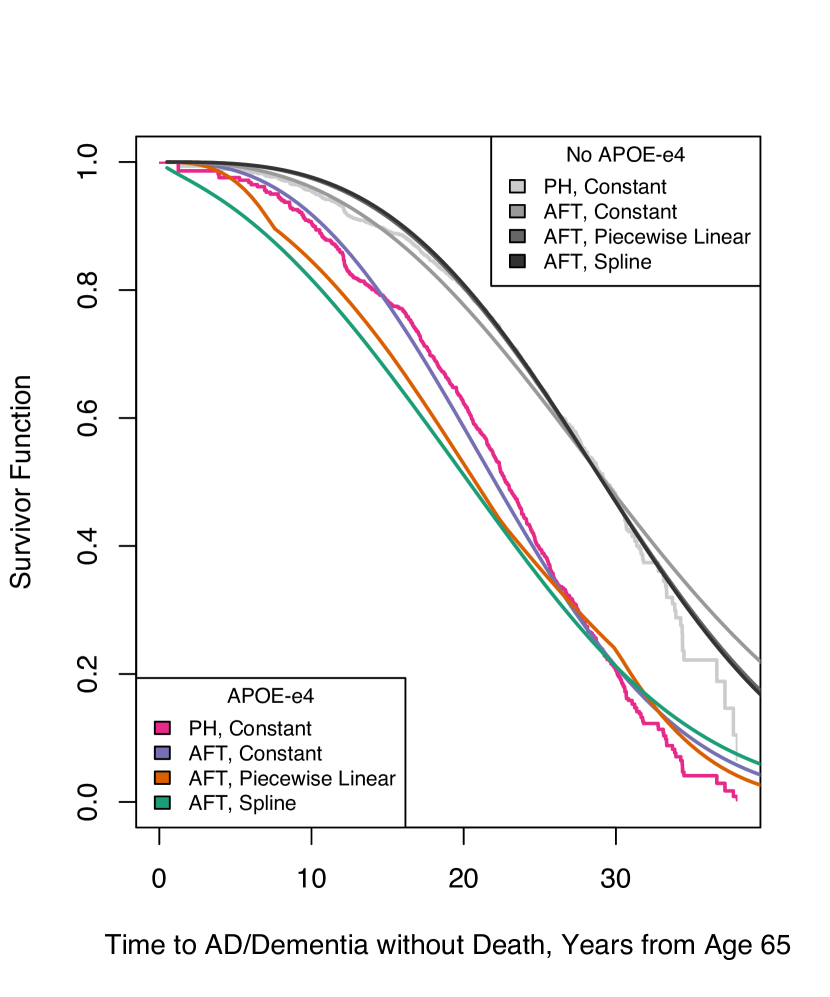
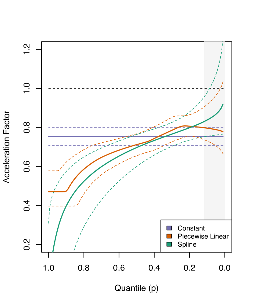
Figure A.1: Under a Weibull baseline specification: (left panel) regression standardized survivor function estimates for onset of AD or dementia without death, averaged over other covariates. Regression standardized estimate from Cox proportional hazards model shown for comparison; (right panel) regression standardized quantile-varying acceleration factor estimates for onset of AD or dementia without death, averaged over other covariates. 95% credible intervals represented with dashed lines. Grey shaded region represents area of parametric extrapolation beyond quantiles observed in both groups.

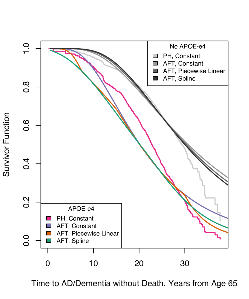
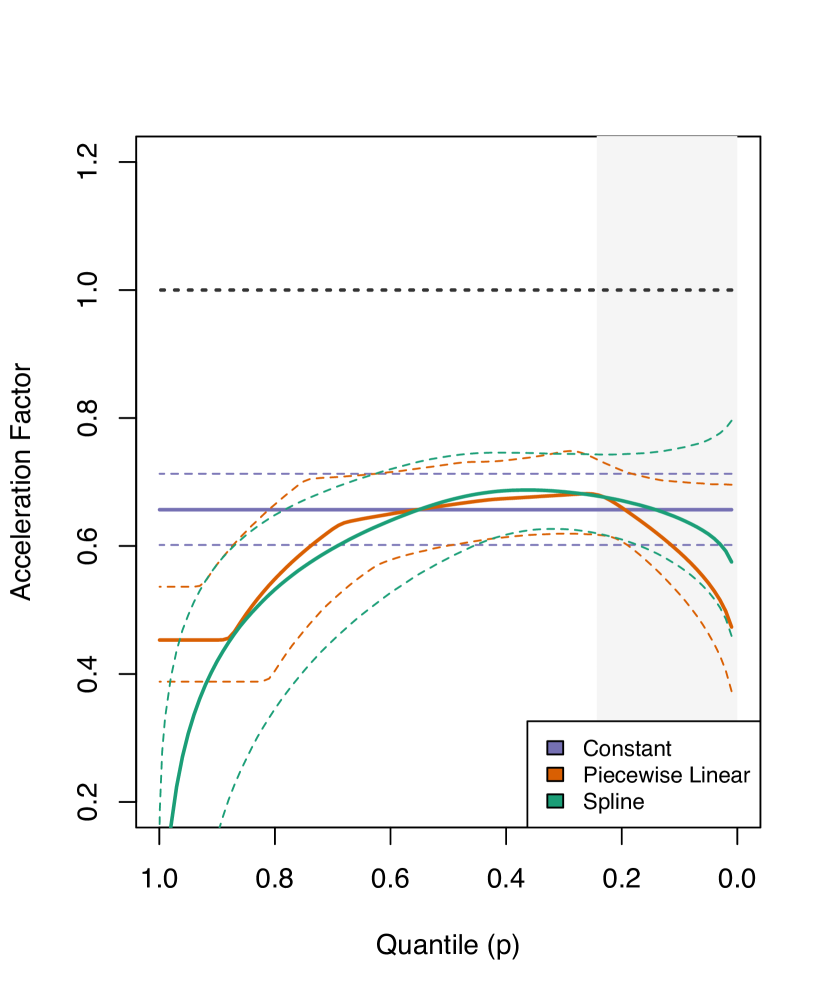
Figure A.2: Under a log-Normal baseline specification: (left panel) regression standardized survivor function estimates for onset of AD or dementia without death, averaged over other covariates. Regression standardized estimate from Cox proportional hazards model shown for comparison; (right panel) regression standardized quantile-varying acceleration factor estimates for onset of AD or dementia without death, averaged over other covariates. 95% credible intervals represented with dashed lines. Grey shaded region represents area of parametric extrapolation beyond quantiles observed in both groups.

A.2 Mortality following AD/Dementia Onset

Below we report regression parameter estimates, and additional regression-standardized survival curves and acceleration factors for mortality by AD/dementia status, across alternative specifications for the baseline distribution.

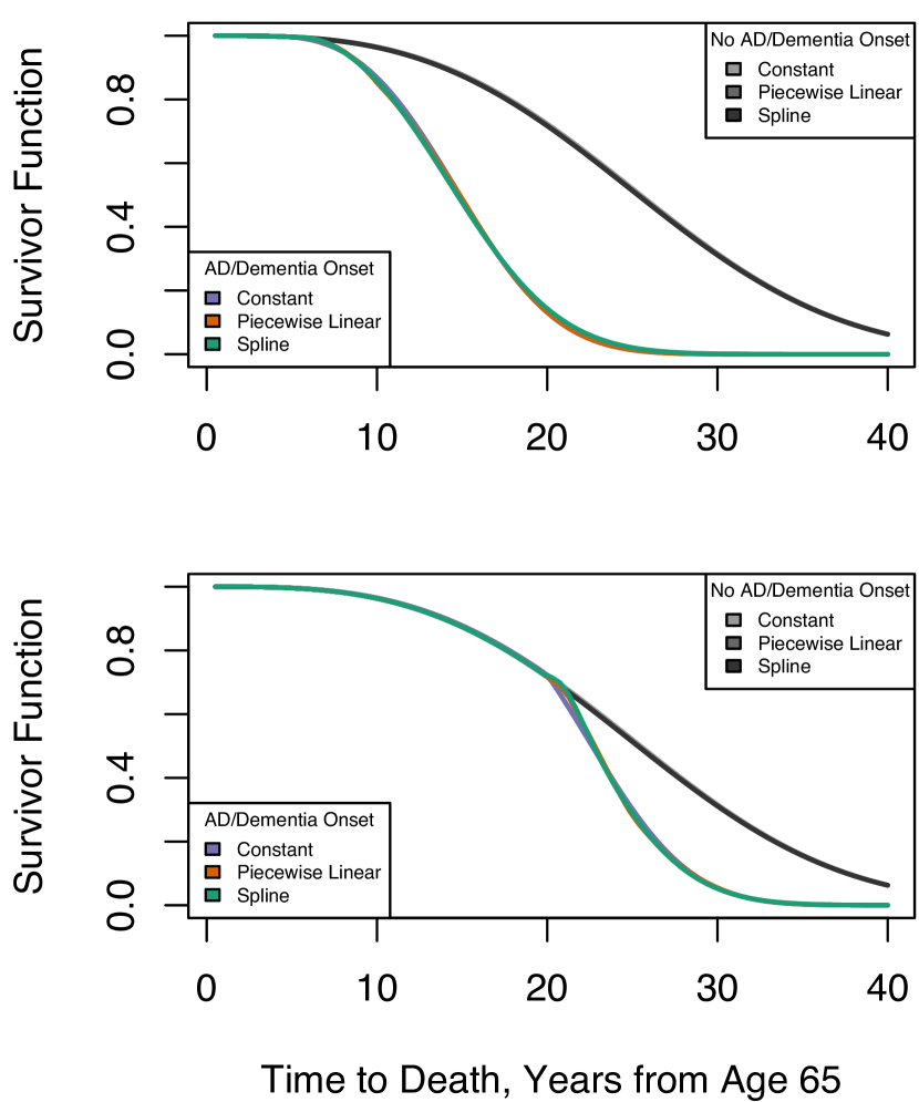
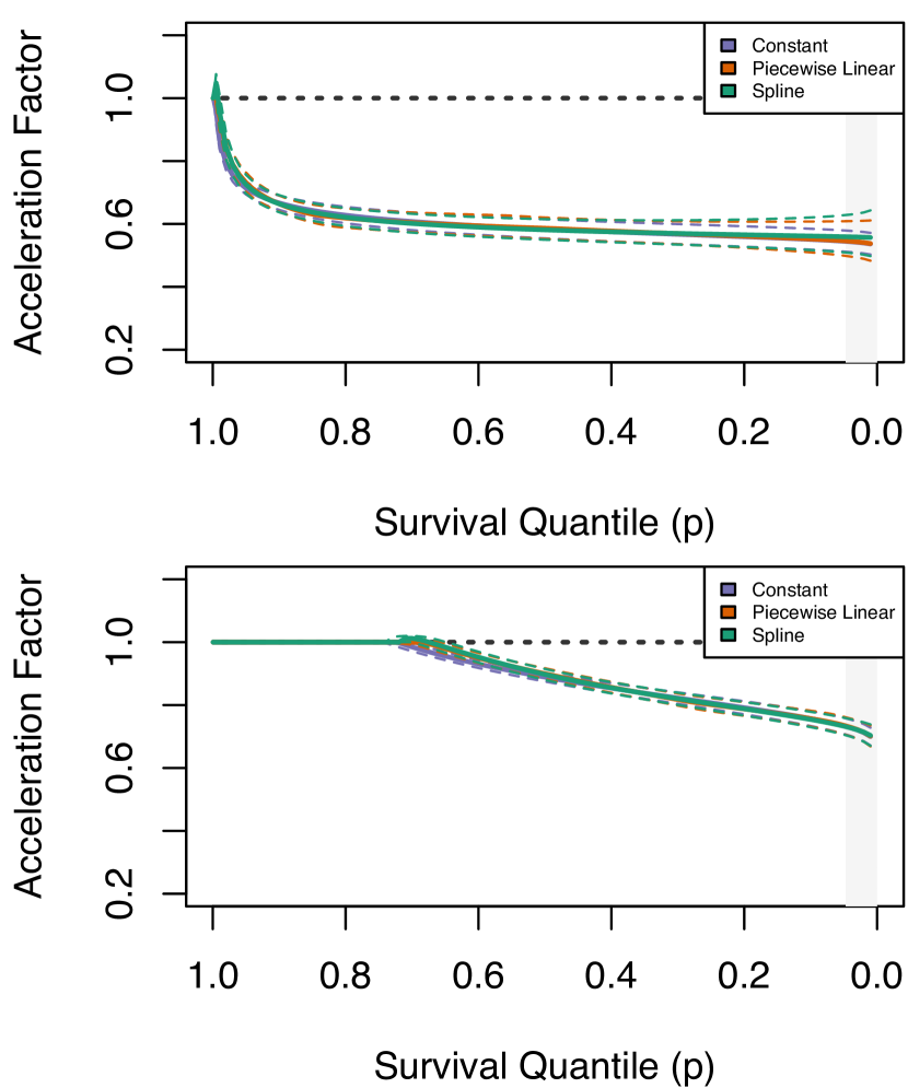
Figure A.3: Under a Weibull baseline specification: (left panel) regression standardized survivor function estimates for mortality following onset of AD or dementia, averaged over other covariates; (Right panel) regression standardized survivor function estimates for mortality following onset of AD or dementia, averaged over other covariates. 95% credible intervals represented with dashed lines. Grey shaded region represents area of parametric extrapolation beyond quantiles observed in both groups.

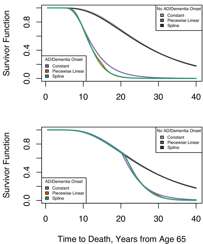
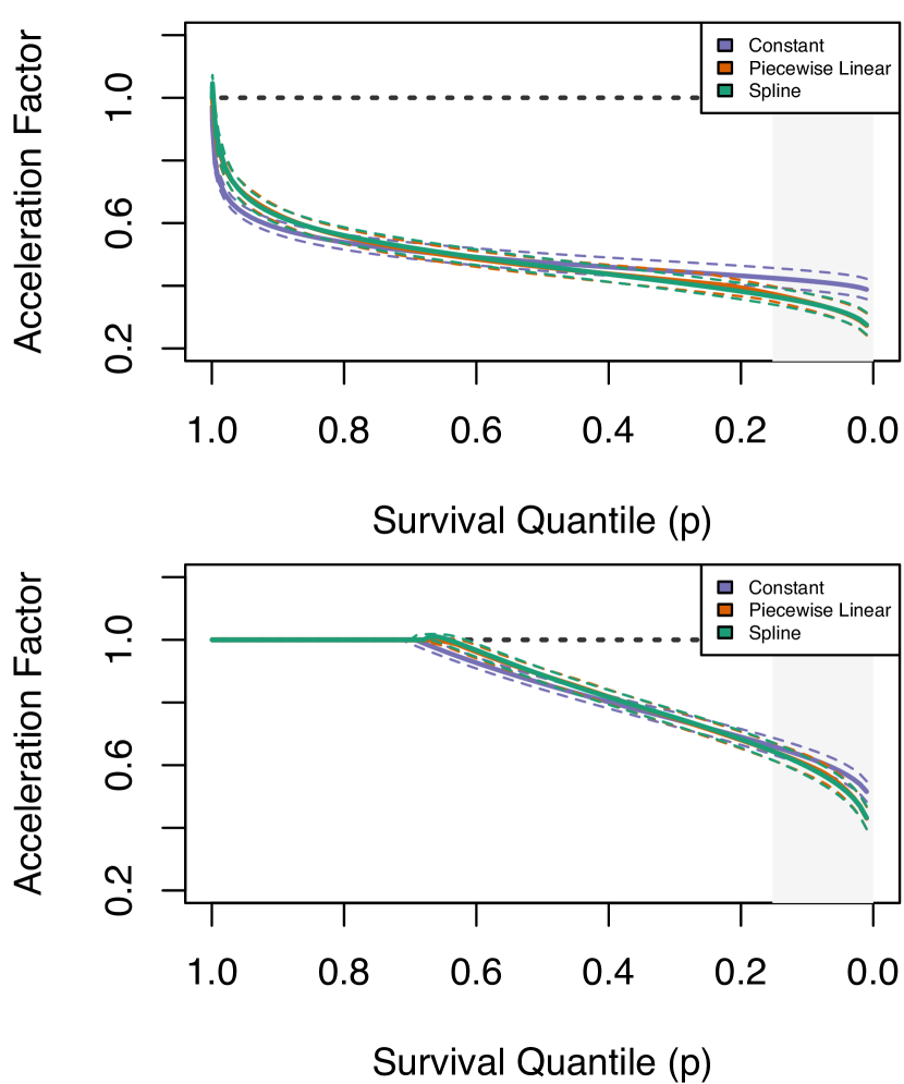
Figure A.4: Under a log-Normal baseline specification: (left panel) regression standardized survivor function estimates for mortality following onset of AD or dementia, averaged over other covariates; (Right panel) regression standardized survivor function estimates for mortality following onset of AD or dementia, averaged over other covariates. 95% credible intervals represented with dashed lines. Grey shaded region represents area of parametric extrapolation beyond quantiles observed in both groups.

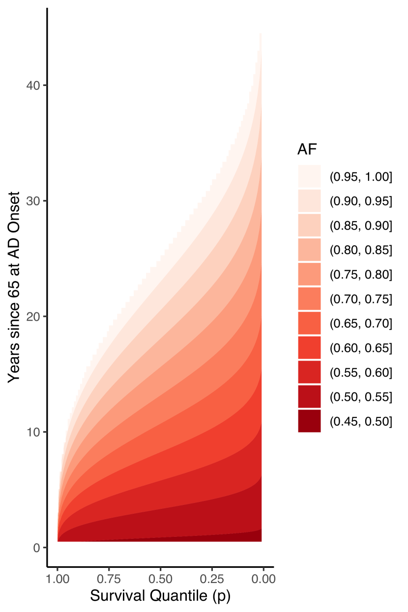
Figure A.5: Under a Weibull baseline specification, contour plots of regression standardized acceleration factor surface estimates for death following onset of AD/dementia, standardized to other covariates. Time of AD/dementia onset is shown on y-axis, and subsequent survival quantile is shown on x-axis. Color indicates acceleration factor at the given survival quantile, comparing those with AD/dementia onset at the specified time and those without AD/dementia. Horizontal cross-sections illustrate quantile-varying acceleration factor for AD/dementia onset at a particular time, while vertical cross-sections illustrate acceleration factor at a particular quantile across times of AD/dementia onset. (Left panel) constant effect specification; (center panel) piecewise linear effect specification; (right panel) spline effect specification.

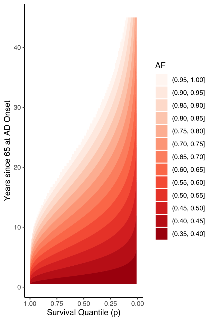
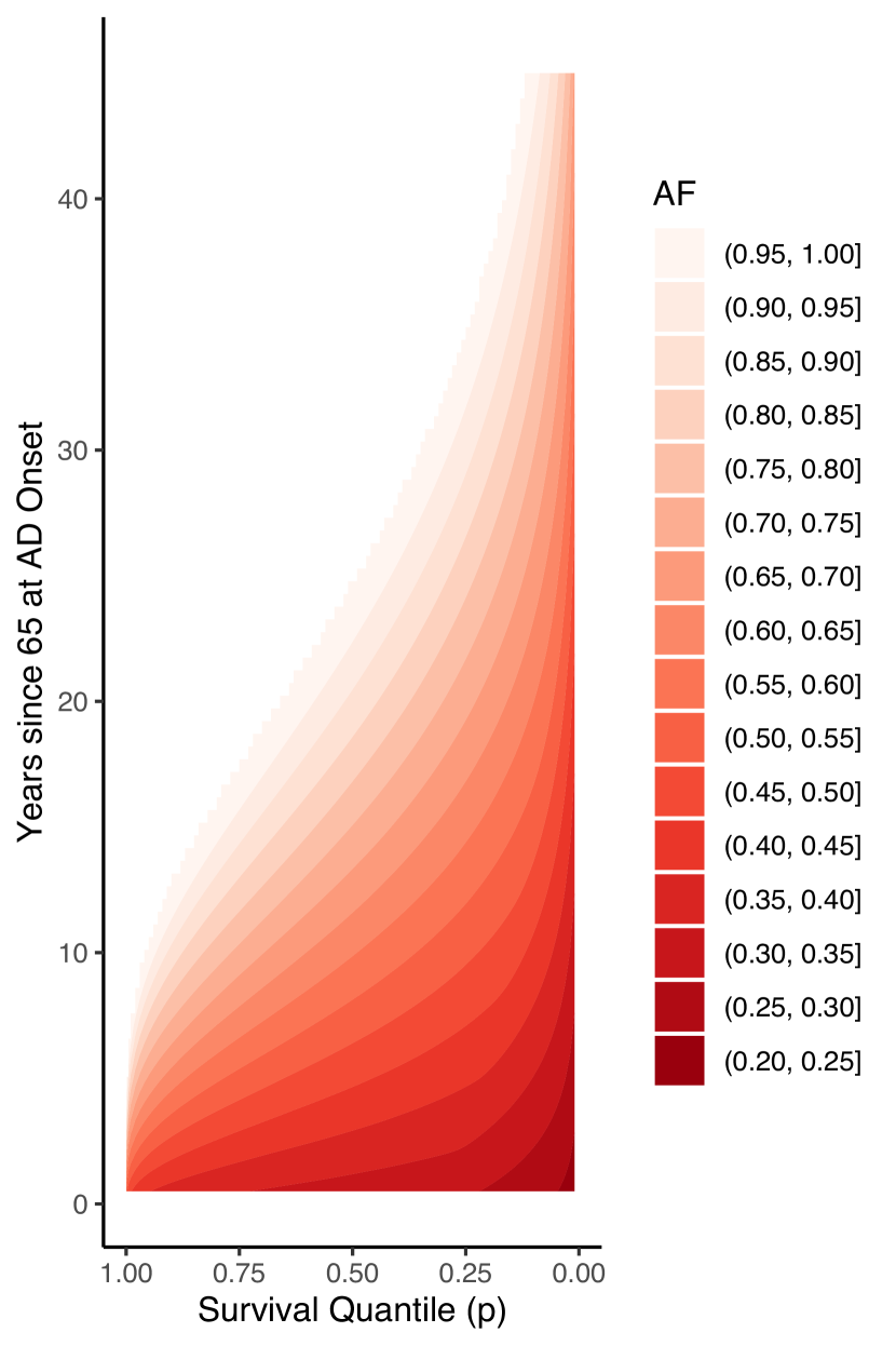
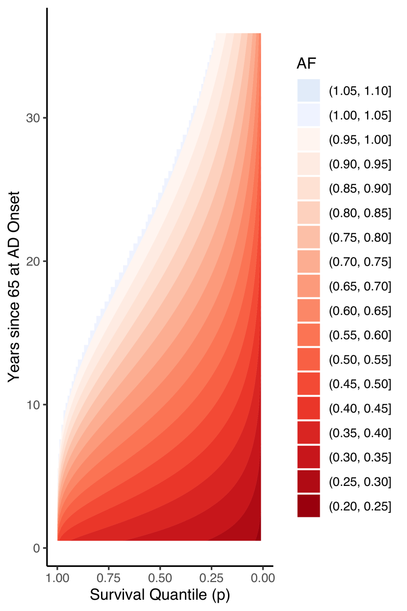
Figure A.6: Under a log-Normal baseline specification, contour plots of regression standardized acceleration factor surface estimates for death following onset of AD/dementia, standardized to other covariates. Time of AD/dementia onset is shown on y-axis, and subsequent survival quantile is shown on x-axis. Color indicates acceleration factor at the given survival quantile, comparing those with AD/dementia onset at the specified time and those without AD/dementia. Horizontal cross-sections illustrate quantile-varying acceleration factor for AD/dementia onset at a particular time, while vertical cross-sections illustrate acceleration factor at a particular quantile across times of AD/dementia onset. (Left panel) constant effect specification; (center panel) piecewise linear effect specification; (right panel) spline effect specification.

Table A.1: Regression estimates for time to death. AFT results are posterior medians and 95% credible intervals for regression parameters. Cox model results are log-hazard ratio estimates and 95% confidence intervals.

		AFT Model
	Cox PH	log-Normal	Weibull	TBP (Weibull Centered)
White Race/Ethnicity, $\beta_{1}$
Constant	0.17 (-0.07, 0.41)	-0.07 (-0.17, 0.03)	-0.08 (-0.16, 0)	-0.07 (-0.14, 0)
Piecewise Linear		-0.1 (-0.21, 0.01)	-0.08 (-0.16, 0)	-0.07 (-0.15, 0.01)
Restricted Cubic Spline		-0.1 (-0.21, 0)	-0.08 (-0.16, 0)	-0.07 (-0.15, 0)
Male Sex, $\beta_{2}$
Constant	0.52 (0.41, 0.64)	-0.25 (-0.31, -0.2)	-0.16 (-0.2, -0.12)	-0.14 (-0.17, -0.11)
Piecewise Linear		-0.27 (-0.33, -0.21)	-0.16 (-0.2, -0.13)	-0.14 (-0.18, -0.11)
Restricted Cubic Spline		-0.27 (-0.33, -0.21)	-0.16 (-0.2, -0.13)	-0.14 (-0.18, -0.11)
Married at Study Entry, $\beta_{3}$
Constant	-0.16 (-0.3, -0.01)	0.12 (0.05, 0.19)	0.05 (0.01, 0.1)	0.04 (0, 0.08)
Piecewise Linear		0.12 (0.05, 0.19)	0.05 (0.01, 0.1)	0.04 (0, 0.08)
Restricted Cubic Spline		0.12 (0.05, 0.19)	0.05 (0.01, 0.1)	0.04 (0, 0.08)
$\geq$15 Years of Education, $\beta_{4}$
Constant	-0.1 (-0.21, 0.01)	0.07 (0.02, 0.13)	0.03 (-0.01, 0.06)	0.02 (-0.01, 0.05)
Piecewise Linear		0.09 (0.03, 0.15)	0.03 (-0.01, 0.07)	0.02 (-0.01, 0.06)
Restricted Cubic Spline		0.09 (0.03, 0.15)	0.03 (0, 0.07)	0.02 (-0.01, 0.06)
APOE-$\epsilon 4$ Genetic Variant, $\beta_{5}$
Constant	0.01 (-0.11, 0.13)	0.06 (0, 0.11)	0.01 (-0.03, 0.05)	0 (-0.03, 0.04)
Piecewise Linear		0.06 (0, 0.12)	0.01 (-0.03, 0.05)	0 (-0.03, 0.04)
Restricted Cubic Spline		0.06 (0, 0.12)	0.01 (-0.03, 0.05)	0 (-0.03, 0.04)
AD/Dementia Onset, $\beta_{6}$
Constant	1.14 (1.02, 1.26)	-1.06 (-1.16, -0.97)	-0.73 (-0.81, -0.65)	-0.68 (-0.76, -0.61)
Piecewise Linear		-0.14 (-0.42, 0.17)	-0.02 (-0.3, 0.29)	0.01 (-0.27, 0.32)
Restricted Cubic Spline		1.59 (0.90, 2.35)	1.63 (0.95, 2.38)	1.68 (1, 2.42)
AD/Dementia Onset, $\alpha_{1}$
Constant
Piecewise Linear		-0.95 (-1.29, -0.63)	-0.86 (-1.21, -0.53)	-0.84 (-1.18, -0.53)
Restricted Cubic Spline		-1.77 (-2.25, -1.33)	-1.60 (-2.08, -1.17)	-1.57 (-2.05, -1.14)
AD/Dementia Onset, $\alpha_{2}$
Constant
Piecewise Linear		-1.15 (-1.49, -0.82)	-0.90 (-1.25, -0.57)	-0.86 (-1.21, -0.54)
Restricted Cubic Spline		-5.07 (-6.56, -3.73)	-4.40 (-5.86, -3.10)	-4.43 (-5.87, -3.11)
AD/Dementia Onset, $\alpha_{3}$
Constant
Piecewise Linear		-1.15 (-1.49, -0.82)	-0.65 (-0.99, -0.33)	-0.62 (-0.96, -0.31)
Restricted Cubic Spline		-1.78 (-2.18, -1.41)	-1.08 (-1.45, -0.75)	-1.08 (-1.44, -0.74)
AD/Dementia Onset, $\alpha_{4}$
Constant
Piecewise Linear		-1.68 (-2.11, -1.26)	-0.71 (-1.10, -0.32)	-0.74 (-1.15, -0.34)
Restricted Cubic Spline

Appendix B Derivation of $V^{-1}(t\mid\mathbf{X})$ under Piecewise Linearity

Under piecewise linear specification of $V(t\mid\mathbf{X})$, define $J+2$ knots $0=\tau_{0}<\tau_{1}<\dots<\tau_{J}<\tau_{J+1}=\infty$, with piecewise linear basis functions defined $B_{j}(t\mid\boldsymbol{\tau})=t^{-1}(\min\{t,\tau_{j+1}\}-\tau_{j})_{+}$ where $(z)_{+}=\min\{0,z\}$. Assuming a flexible effect for $X_{1}$, the resulting specification becomes

$$V(t\mid\mathbf{X})=t\times\exp\left(-\mathbf{X}^{{\mathsf{\scriptscriptstyle T}}}\boldsymbol{\beta}\right)\left[\sum_{j=1}^{J}\exp\left(-X_{1}\alpha_{j}\right)B_{j}(t\mid\boldsymbol{\tau})\right].$$ (B.1)

The inverse function $V^{-1}$ can be derived by inspection, noting that the inverse of an increasing piecewise linear function is also an increasing piecewise linear function, with changepoints shifted according to the values of $\mathbf{X}$, $\boldsymbol{\beta}$, and $\boldsymbol{\alpha}$. Specifically, define $\boldsymbol{\tau}^{*}$ such that $\tau_{0}^{*}=\tau_{0}=0$, $\tau_{1}^{*}=\tau_{1}\times\exp(-\mathbf{X}^{{\mathsf{\scriptscriptstyle T}}}\boldsymbol{\beta})$, and for $j>1$,

$$\tau^{*}_{j} =\tau^{*}_{1}+\sum_{l=2}^{j}\exp(-\mathbf{X}^{{\mathsf{\scriptscriptstyle T}}}\boldsymbol{\beta}-X_{1}\alpha_{l-1})(\tau_{l}-\tau_{l-1}).$$ (B.2)

The lines on each interval of $V^{-1}$ have the inverse slope of the line in the corresponding interval of $V$, so the final inverse function is succinctly written

$$V^{-1}(t\mid\mathbf{X})=t\times\exp\left(\mathbf{X}^{{\mathsf{\scriptscriptstyle T}}}\boldsymbol{\beta}\right)\left[\sum_{j=1}^{J}\exp\left(X_{1}\alpha_{j}\right)B_{j}(t\mid\boldsymbol{\tau}^{*})\right].$$ (B.3)

Appendix C Derivation of Acceleration Factor for a Binary Time-Varying Covariate

Let $X_{1}(t)$ be a binary-valued step function, such as an indicator for whether a non-terminal event has occurred by time $t$. Formally, define $X_{1}(t)=\mathbb{I}(t>t_{X})$, where $t_{X}$ is the time at which $X_{1}$ changes. Consider a single additional covariate time-invariant covariate $X_{2}$.

Notating $t_{X}^{*}=t_{X}\exp(-X_{2}\beta_{2})$, the inverse function for $V$ as defined in (21) is derived following Appendix B as

$$V^{-1}(t\mid\mathbf{X}(t)) =\exp\left(X_{2}\beta_{2}\right)\left[\min\{t,t_{X}^{*}\}+(t-t_{X}^{*})_{+}\exp\left(\beta_{1}\right)\right].$$ (C.1)

The resulting acceleration factor at quantile $p$ between a person with $X_{2}=x_{2}$ who experiences the non-terminal event at time $t_{X}$, and a person with $X_{2}=x^{\prime}_{2}$ who experiences the non-terminal event at time $t^{\prime}_{X}$, is

$$\xi(p\mid t_{X},t_{X}^{\prime},x_{2},x^{\prime}_{2},S_{0}) =e^{(x_{2}-x^{\prime}_{2})\beta_{2}}\frac{\min\{S^{-1}_{0}(p),t_{X}e^{-x_{2}\beta_{2}}\}+e^{\beta_{1}}(S^{-1}_{0}(p)-t_{X}e^{-x_{2}\beta_{2}})_{+}}{\min\{S^{-1}_{0}(p),t_{X}^{\prime}e^{-x^{\prime}_{2}\beta_{2}}\}+e^{\beta_{1}}(S^{-1}_{0}(p)-t_{X}^{\prime}e^{-x^{\prime}_{2}\beta_{2}})_{+}}.$$ (C.2)

Finally, note that when a general flexible effect for $X_{1}(t)$ is specified, in general no closed form exists, but acceleration factors can still be computed numerically.

Appendix D Transformed Bernstein Polynomial Prior

To illustrate the flexibility of the transformed Bernstein polynomial prior, Figure D.1 shows the basis functions when $K=5$,

$$G(p\mid k,K-k+1)=\frac{\Gamma(K+1)}{\Gamma(k)\Gamma(K-k+1)}p^{k-1}(1-p)^{K-k}.$$

Moreover, Figure D.2 shows a sample of different shapes that the resulting baseline survivor function $S_{0}(t\mid\boldsymbol{\phi},\mathbf{w})=\sum_{k=1}^{K}w_{k}G(S^{*}_{0}(t\mid\boldsymbol{\phi})\mid k,K-k+1)$ can take, for selected weight vectors $\mathbf{w}$ and setting $S^{*}_{0}(t)=\exp(-t)$.

Figure D.1: Basis functions $G$ for $j=1,\dots,5$.

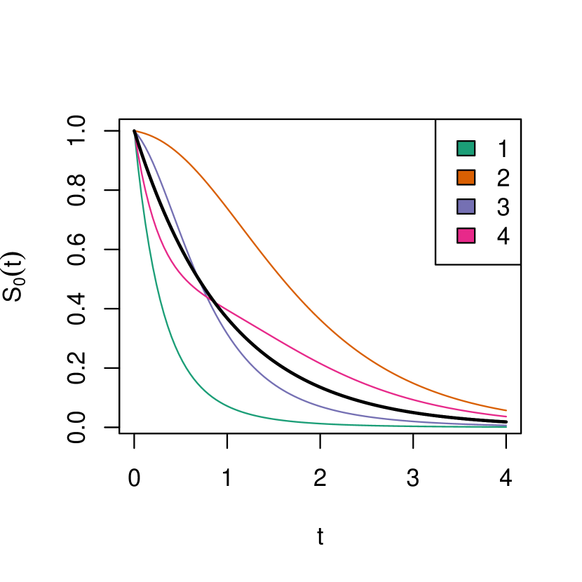
	1	2	3	4
$w_{1}$	0.01	0.64	0.07	0.41
$w_{2}$	0.03	0.23	0.18	0.02
$w_{3}$	0.09	0.09	0.50	0.01
$w_{4}$	0.23	0.03	0.18	0.15
$w_{5}$	0.64	0.01	0.07	0.41

Figure D.2: Sample survivor functions corresponding to varying transformed bernstein polynomial prior weight vectors. Bold black line shows centering distribution $S_{0}^{*}(t)=\exp(-t)$.

References

- Bennett et al., (2018) Bennett, D. A., Buchman, A. S., Boyle, P. A., Barnes, L. L., Wilson, R. S., and Schneider, J. A. (2018). Religious Orders Study and Rush Memory and Aging Project. Journal of Alzheimer’s Disease, 64(s1):S161–S189.
- Carpenter et al., (2017) Carpenter, B., Gelman, A., Hoffman, M. D., Lee, D., Goodrich, B., Betancourt, M., Brubaker, M., Guo, J., Li, P., and Riddell, A. (2017). Stan: A Probabilistic Programming Language. Journal of Statistical Software, 76(1).
- Cox and Oakes, (1984) Cox, D. R. and Oakes, D. (1984). Analysis of Survival Data. Monographs on Statistics and Applied Probability. Chapman and Hall, London ; New York.
- Crowther et al., (2022) Crowther, M. J., Royston, P., and Clements, M. (2022). A flexible parametric accelerated failure time model and the extension to time-dependent acceleration factors. Biostatistics, page kxac009.
- Haneuse et al., (2008) Haneuse, S. J.-P. A., Rudser, K. D., and Gillen, D. L. (2008). The separation of timescales in Bayesian survival modeling of the time-varying effect of a time-dependent exposure. Biostatistics, 9(3):400–410.
- Hanson et al., (2009) Hanson, T., Johnson, W., and Laud, P. (2009). Semiparametric inference for survival models with step process covariates. Canadian Journal of Statistics, 37(1):60–79.
- Hernán, (2010) Hernán, M. A. (2010). The hazards of hazard ratios. Epidemiology, 21(1):13–15.
- Keil et al., (2018) Keil, A. P., Daza, E. J., Engel, S. M., Buckley, J. P., and Edwards, J. K. (2018). A Bayesian approach to the g-formula. Statistical Methods in Medical Research, 27(10):3183–3204.
- Kukull et al., (2002) Kukull, W. A., Higdon, R., Bowen, J. D., McCormick, W. C., Teri, L., Schellenberg, G. D., van Belle, G., Jolley, L., and Larson, E. B. (2002). Dementia and Alzheimer disease incidence: A prospective cohort study. Archives of Neurology, 59(11):1737.
- Lee et al., (2017) Lee, K. H., Rondeau, V., and Haneuse, S. (2017). Accelerated failure time models for semi-competing risks data in the presence of complex censoring. Biometrics, 73(4):1401–1412.
- Pang et al., (2021) Pang, M., Platt, R. W., Schuster, T., and Abrahamowicz, M. (2021). Flexible extension of the accelerated failure time model to account for nonlinear and time-dependent effects of covariates on the hazard. Statistical Methods in Medical Research, 30(11):2526–2542.
- Portnoy, (2003) Portnoy, S. (2003). Censored regression quantiles. Journal of the American Statistical Association, 98(464):1001–1012.
- Prentice and Kalbfleisch, (1979) Prentice, R. L. and Kalbfleisch, J. D. (1979). Hazard rate models with covariates. Biometrics, 35(1):25.
- Reich and Smith, (2013) Reich, B. J. and Smith, L. B. (2013). Bayesian quantile regression for censored data. Biometrics, 69(3):651–660.
- Rothman et al., (2021) Rothman, K. J., Lash, T. L., VanderWeele, T. J., and Haneuse, S. (2021). Modern Epidemiology. Wolters Kluwer, Philadelphia, fourth edition edition.
- Royston and Parmar, (2002) Royston, P. and Parmar, M. K. B. (2002). Flexible parametric proportional-hazards and proportional-odds models for censored survival data, with application to prognostic modelling and estimation of treatment effects. Statistics in Medicine, 21(15):2175–2197.
- Sjölander, (2016) Sjölander, A. (2016). Regression standardization with the R package stdReg. European Journal of Epidemiology, 31(6):563–574.
- Stan Development Team, (2020) Stan Development Team (2020). RStan: The R interface to Stan.
- Uno et al., (2015) Uno, H., Wittes, J., Fu, H., Solomon, S. D., Claggett, B., Tian, L., Cai, T., Pfeffer, M. A., Evans, S. R., and Wei, L.-J. (2015). Alternatives to hazard ratios for comparing the efficacy or safety of therapies in noninferiority studies. Annals of Internal Medicine, 163(2):127–134.
- Vehtari et al., (2017) Vehtari, A., Gelman, A., and Gabry, J. (2017). Practical Bayesian model evaluation using leave-one-out cross-validation and WAIC. Statistics and Computing, 27(5):1413–1432.
- Wei, (1992) Wei, L. J. (1992). The accelerated failure time model: A useful alternative to the cox regression model in survival analysis. Statistics in Medicine, 11(14-15):1871–1879.
- Zhou and Hanson, (2018) Zhou, H. and Hanson, T. (2018). A unified framework for fitting bayesian semiparametric models to arbitrarily censored survival data, including spatially referenced data. Journal of the American Statistical Association, 113(522):571–581.