Analyzing the Representational Geometry of Acoustic Word Embeddings

Abstract

Acoustic word embeddings (AWEs) are vector representations such that different acoustic exemplars of the same word are projected nearby in the embedding space. In addition to their use in speech technology applications such as spoken term discovery and keyword spotting, AWE models have been adopted as models of spoken-word processing in several cognitively motivated studies and have been shown to exhibit human-like performance in some auditory processing tasks. Nevertheless, the representational geometry of AWEs remains an under-explored topic that has not been studied in the literature. In this paper, we take a closer analytical look at AWEs learned from English speech and study how the choice of the learning objective and the architecture shapes their representational profile. To this end, we employ a set of analytic techniques from machine learning and neuroscience in three different analyses: embedding space uniformity, word discriminability, and representational consistency. Our main findings highlight the prominent role of the learning objective on shaping the representation profile compared to the model architecture.

Analyzing the Representational Geometry of Acoustic Word Embeddings

Badr M. Abdullah  and Dietrich Klakow Language Science and Technology (LST), Saarland University, Germany Saarland Informatics Campus { babdullah | dietrich }@lsv.uni-saarland.de

1 Introduction

Due to their ubiquity, word embeddings are nowadays a central component in natural language processing (NLP). Inducing word embeddings from text yields representations such that words occurring in similar contexts are nearby in the vector space Mikolov et al. (2013); Pennington et al. (2014). Therefore, the representational geometry of text-based word embeddings captures lexical similarity and semantic relatedness at multiple levels of granularity. Word embeddings, and their underlying distributional semantic models, have also been adopted as models of human semantic memory in cognitive science research (Pereira et al., 2016; Nematzadeh et al., 2017; Grand et al., 2022).

In the speech processing domain, researchers have independently developed representations of acoustic segments that correspond to linguistic units (Levin et al., 2013; Bengio and Heigold, 2014; Kamper et al., 2016b; Settle and Livescu, 2016a, inter alia). A notable example of such representations are acoustic word embeddings (AWEs)—vector representations that encode the sound structure of words, not their semantic and syntactic structure—see Fig. 1. AWEs support voice-based speech technology applications such as query-by-example spoken term discovery  Zhang and Glass (2009); Jansen and Durme (2012); Metze et al. (2013) and keyword spotting Myers et al. (1980); Rohlicek (1995). In addition, AWEs can be leveraged to facilitate access to speech recordings of endangered spoken languages that might lack standardized writing systems Bird (2021); San et al. (2021)

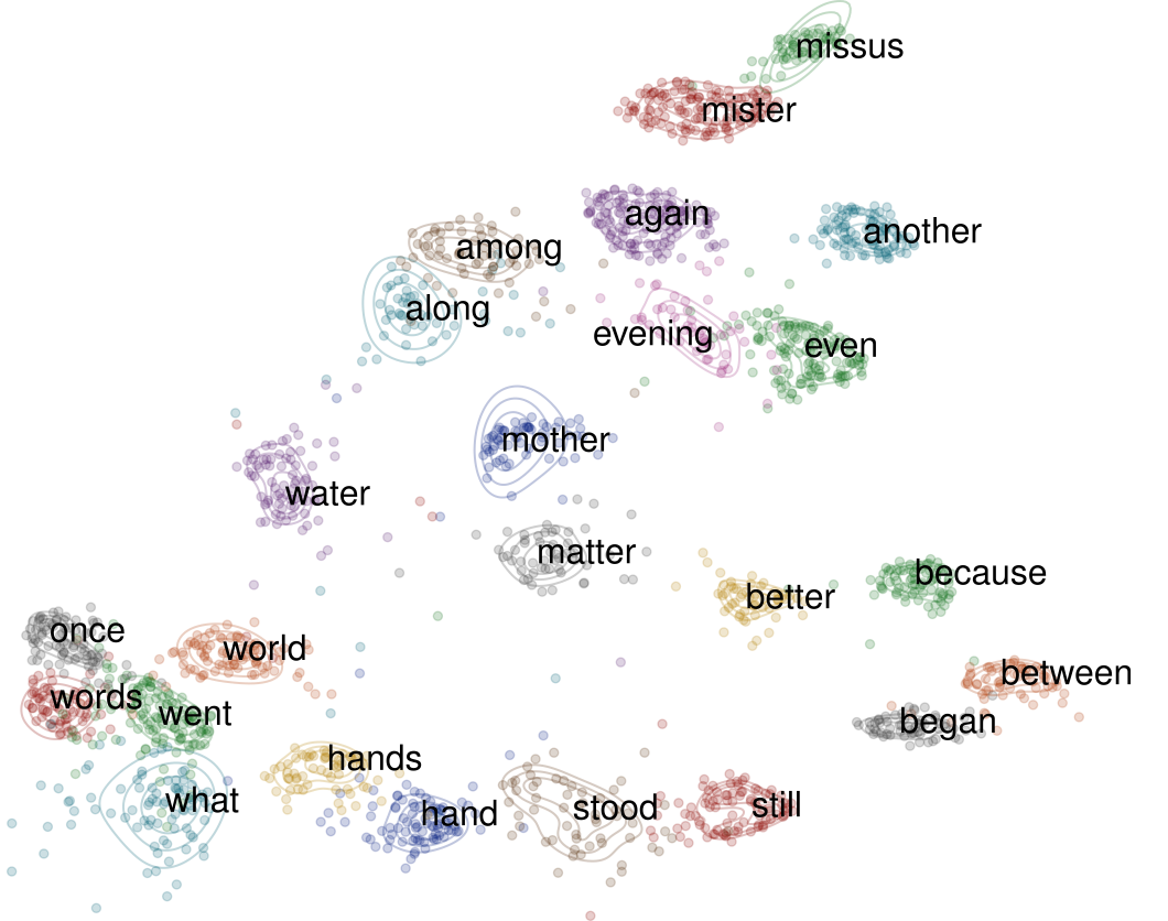
Figure 1: UMAP projection (McInnes et al., 2018) of a sample of acoustic word embeddings (AWEs) produced by a correspondence autoencoder (CAE) model trained on English read speech. AWE models project different exemplars of the same word type closer in the embedding space while abstracting away from speaker and context variability.

However, there are fundamental differences between text-based and speech-based word embeddings that have to do with the degree of variability between the two modalities. Contrary to written words which have context-invariant orthographic realizations, spoken words are notoriously variable. The underlying sources of variability in speech include speaker-related factors such as vocal tract shape, gender, age, and dialect. In addition, two acoustic instances, or exemplars, of the same word will vary in different phonological and semantic contexts even if they are produced by the same speaker Jurafsky (2003). Therefore, acoustic word embeddings are not static, but have to be computed “on the fly” given a speech segment as input. Models of AWEs need to abstract away from speaker and context variability to project different acoustic exemplars of the same word onto (ideally) the same point of the embedding space.

Nevertheless, AWEs have not yet been extensively studied in the literature from a neural network interpretability point of view. We are only aware of a few prior efforts in this direction that have either analyzed the representational geometry of AWEs from a cognitively motivated angle Matusevych et al. (2020a); Abdullah et al. (2021a) or from a cross-linguistic perspective Abdullah et al. (2021b). In this paper, we make a contribution in this direction and use analytic techniques from machine learning and neuroscience in three different analytic studies: embedding space uniformity (§4), word discriminability (§5), and representational consistency (§6).

2 Acoustic Word Embedding Models

Given an acoustic signal that corresponds to a spoken word represented as a temporal sequence of $T$ acoustic feature vectors, i.e., ${\boldsymbol{a}}=(\boldsymbol{a}^{1},\boldsymbol{a}^{2},...,\boldsymbol{a}^{T})$, the goal of an AWE model is to transform $\boldsymbol{a}$ into a fixed-dimensionality vector representation $\mathbf{e}$. Due to the variability in speech production (i.e., speech rate, emotional state, etc), the length of the acoustic segment $T$ varies between different exemplars, or instances, of the same word type. Therefore, this task is modeled as a mapping $\mathcal{F}:\mathcal{A}\xrightarrow[]{}\mathbb{R}^{D}$, where $\mathcal{A}$ is the (continuous) space of acoustic sequences and $D$ is the dimensionality of the embedding. Formally, transforming a variable-length acoustic input into a $D$-dimensional AWE is described as

$$\mathbf{e}=\mathcal{F}(\boldsymbol{a};\boldsymbol{\theta}_{\mathcal{F}})\in\mathbb{R}^{D}$$ (1)

where $\boldsymbol{\theta}_{\mathcal{F}}$ are the parameters of the encoder function $\mathcal{F}$. In a supervised setting of training AWE models, one assumes a dataset $\mathcal{D}=\{(\boldsymbol{a}_{1},w_{1}),(\boldsymbol{a}_{2},w_{2}),\dots,(\boldsymbol{a}_{N},w_{N})\}$ of $N$ spoken word instances where $w_{i}$ is the word type, or lexical category, of the $i$th acoustic sample. In this paper, we experiment with two architectural choices—recurrent and convolutional—and employ four different learning objectives for training AWE models from the literature. Next, we formally describe each of the objectives.

2.1 Correspondence Autoencoder

In the correspondence autoencoder (CAE) Kamper (2019), each training acoustic word sample ${\boldsymbol{a}}$ is paired with another sample that corresponds to the same word type ${\boldsymbol{a}_{+}=(\boldsymbol{a}^{1}_{+},\boldsymbol{a}^{2}_{+},...,\boldsymbol{a}_{+}^{S}})$. The acoustic encoder $\mathcal{F}$ takes ${\boldsymbol{a}}$ as input and produces an embedding $\mathbf{e}$, which is then fed to an acoustic decoder $\mathcal{H}$ that aims to sequentially reconstruct the corresponding acoustic sequence $\boldsymbol{a}_{+}$—see Fig. 6(a). The objective is to minimize the $L_{2}$ distance at each timestep in the decoder, which is equivalent to

$$J=\sum_{i=1}^{S}{\lVert\boldsymbol{a}^{i}_{+}-\mathcal{H}^{i}(\mathbf{e})\rVert_{2}}$$ (2)

where $\boldsymbol{a}_{i}^{+}$ is the ground-truth acoustic feature vector at timestep $i$ and $\mathcal{H}_{i}(\mathbf{e})$ is the reconstructed acoustic vector at timestep $i$ as a function of the embedding $\mathbf{e}$. Learning the correspondence between different acoustic realizations of the same word type seems to encourage the encoder to build up speaker-invariant word representations while preserving linguistically-relevant phonetic information Matusevych et al. (2020b). When the target acoustic sequence to generate is the same as the input signal $\boldsymbol{a}$, this corresponds to a conventional autoencoder (AE) which we consider as one of our learning objectives in this paper.

2.2 Phonologically Guided Encoder

The phonologically guided encoder (PGE) is trained as component in a sequence-to-sequence model to map acoustics into phonology Abdullah et al. (2021a). Given the output of the encoder as an embedding $\mathbf{e}$, a phonological decoder $\mathcal{G}(.;\boldsymbol{\theta}_{\mathcal{G}})$ is trained to decode the corresponding phonological sequence $\boldsymbol{\varphi}=(\varphi^{1},\dots,\varphi^{\tau})$ of the word-form —see Fig. 6(b). The objective is to minimize a categorical cross-entropy loss at each decoder timestep, which is equivalent to minimizing the term

$$J =-\sum_{({\boldsymbol{a}}_{i},w_{i})\in\mathcal{D}}{\text{log }\mathbf{P}\big{(}\boldsymbol{\varphi}|\mathbf{e}_{i};\boldsymbol{\theta}_{\mathcal{G}}\big{)}}$$ (3)

$$=-\sum_{({\boldsymbol{a}}_{i},w_{i})\in\mathcal{D}}\sum_{t=1}^{\tau}{\text{log }\mathbf{P}\big{(}\varphi^{t}|t,\mathbf{e}_{i};\boldsymbol{\theta}_{\mathcal{G}}\big{)}}$$

where $\mathbf{P}\big{(}\varphi^{t}|t,\mathbf{e}_{i};\boldsymbol{\theta}_{\mathcal{G}}\big{)}$ is the probability of the phoneme $\varphi^{t}$ at the $t$th timestep, conditioned on the previous phoneme sequence $\boldsymbol{\varphi}^{<t}$ and the AWE $\mathbf{e}$, and $\boldsymbol{\theta}_{\mathcal{G}}$ are the parameters of the decoder. The intuition of this learning objective is the following: although their acoustic realizations vary due to speaker and context variability, different exemplars of the same word category would have identical phonological sequences. We thus expect the encoder to project exemplars of the same lexical category nearby in the embedding space while embedding similarity in the vector space should correlate with phonological similarity.

2.3 Contrastive Siamese Encoder

The contrastive siamese encoder (CSE) has been explored in the context of AWEs with both recurrent and convolutional architectures in several studies Settle and Livescu (2016b); Kamper et al. (2016a); Jacobs et al. (2021). Contrary to the previously described objectives, the CSE explicitly minimizes the distance between exemplar embeddings of the same word type—see Fig. 6(c). First, each acoustic word instance is paired with another instance of the same word type $(\boldsymbol{a},\boldsymbol{a}_{+})$. Given their embeddings $(\mathbf{e}_{a},\mathbf{e}_{+})$, the objective is then to minimize a triplet margin loss

$$J=\text{max}\big{[}0,m+d(\mathbf{e}_{a},\mathbf{e}_{+})-d(\mathbf{e}_{a},\mathbf{e}_{-})\big{]}$$ (4)

Here, $d(.,.)$ is the cosine distance and $\mathbf{e}_{-}$ is an AWE that corresponds to a different word type sampled from the mini-batch such that the term $d(\mathbf{e}_{a},\mathbf{e}_{-})$ is minimized. This objective clusters acoustic instances of the same word type closer in the embedding space while pushing away instances of other word types by a distance defined by the margin hyperparameter $m$.

3 Data, Setup, and Intrinsic Evaluation

3.1 Experimental Data

The data in our study is drawn from the the LibriSpeech dataset which contains read speech recordings of American-English Panayotov et al. (2015), which is a public dataset under the CC BY 4.0 license. We sample 384 speakers from for training and 128 for evaluation—disjoint sets—and obtain word-aligned speech samples using the Montreal Forced Aligner McAuliffe et al. (2017). To make our models comparable with prior work, which has focused on AWEs for low-resource languages, we sample $\sim 39.4$k samples for training and $\sim 9.7$k for evaluation. The phonetic transcription for each word is produced using the online WebMaus G2P tool Strunk et al. (2014). Then, each acoustic segment is parametrized as a sequence of 39-dimensional Mel-frequency spectral coefficients of 25ms frames with 15ms overlap—the conventional feature representation of speech in automatic speech recognition (ASR). It is worth pointing out that in this paper we consider each morphological variant of a lexeme as a separate lexical category. For example, different inflections of the lexeme make such as {made, making, maker, etc.} represent different lexical categories, each with its own exemplars.

3.2 Architectures, Hyperparameters, and Training Details

CNN Acoustic Encoder.    We employ a 3-layer temporal convolutional network (1D-CNN) with 256, 384, and 512 filters and widths of 4, 8, and 16 for each layer and keep stride step at 1. Following each convolutional operation, we apply batch normalization, ReLU non-linearity, and dropout. We apply average pooling to downsample the representation at the end of the convolution block, then apply one non-linear layer with Tanh on the CNN output, which yields a 512-dimensional AWE.

RNN Acoustic Encoder.    We employ a 3-layer directional Gated Recurrent Unit (GRU) with a hidden state dimension of 512, then apply one non-linear layer with Tanh on the GRU output, which yields a 512-dimensional AWE. We apply layer-wise dropout with a probability of $0.1$.

Phonological Decoder $\mathcal{G}(.;\boldsymbol{\theta}_{\mathcal{G}})$.   We employ a 1-layer GRU of 512 units hidden state that takes the 512-dimensional AWE as the initial hidden state and decodes the corresponding phonological sequence without teacher forcing.

Acoustic Decoder $\mathcal{H}(.;\boldsymbol{\theta}_{\mathcal{H}})$.   We employ a 1-layer GRU of 512 units hidden state that takes the 512-dimensional AWE as the initial hidden state and decodes the corresponding acoustic sequence with a teacher forcing ratio of 0.2.

Contrastive Loss.   For the CSE, we experiment with different values of the margin hyperparameter $m=\{0.2,0.3,0.4,0.5\}$, out of which $0.4$ yields the best performance on the validation set.

Training Details.    All models in this study are randomly initialized with each parameter drawn uniformly from $[-0.05,0.05]$. Then, each model is trained for 100 epochs with a batch size of 256 using the ADAM optimizer Kingma and Ba (2015) and an initial learning rate of 0.001. The learning rate is reduced by a factor of 0.5 if the mAP on the validation set does not improve for 10 epochs.

Implementation.    We build our models using PyTorch Paszke et al. (2019) and use FAISS Johnson et al. (2017) for efficient similarity search. Our code is based on our prior work in building and analyzing AWEs Abdullah et al. (2021a, b).

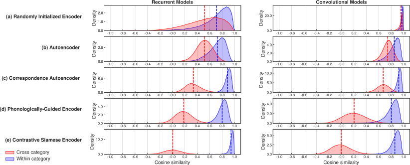
Figure 2: Distribution of cosine similarity scores of the different models for within category samples (i.e., exemplar pairs of the same word type) and cross-category samples (i.e., sample pairs that correspond to different word types). Each row in the figure corresponds to one learning objective and each column corresponds to one architecture.

3.3 Quantitative Evaluation

We conduct an intrinsic evaluation for the AWEs to assess the performance of our models using the same-different acoustic word discrimination task with the mean average precision (mAP) metric Carlin et al. (2011); Kamper et al. (2015); Settle et al. (2019); Algayres et al. (2020). This task evaluates the ability of the model to determine whether two given speech segments correspond to the same word type—that is, whether or not two acoustic segments are exemplars of the same category. The results of the evaluation is shown in Fig. 7 in the appendix. We observe that each recurrent encoder outperforms its convolutional counterpart within each objective. Moreover, the performance largely depends on the strength of the supervision signal where the contrastive encoders outperform other objectives that lack explicit loss to group exemplars of the same category closer in the embedding space.

4 Analysis 1: Embedding Space Uniformity

In our first analysis, we take a closer look at how uniform are representational spaces of AWE models by analyzing the distribution of cosine similarity for each model type and the degree to which the embeddings are isotropic.

4.1 Distribution of Cosine Similarity

One way of analyzing the geometry of representation spaces in the acoustic domain is by inspecting the similarity distributions of exemplars of the same lexical category (or word type) versus randomly sampled, cross-category exemplars. We perform this analysis on the training samples and depict the result in Fig. 2. We observe that the difference between the means of the within-category and those of cross-category distributions is largely dependent on the strength of the supervision signal with the randomly initialized encoders (RIE) having the smallest mean differences for both architectures. The contrastive encoders have the largest mean difference–with mean cross-category scores centered at the zero—which is intuitive given the explicit supervision signal they receive in grouping exemplars of the same category closer in the embedding space. One surprising observation is the behavior of the untrained convolutional encoder which gives cosine similarity scores very close to 1 for each input pair. In appendix C, we demonstrate that this behavior is mainly caused by the unbounded activation function (i.e., ReLU) in the convolutional layers.

4.2 Degree of Isotropy

Although inspecting the cosine similarity distributions is an insightful analysis, it does not enable us to make well-informed judgments about the uniformity of the representation spaces. Here, we ask two questions: (1) do AWE models utilize all dimensions of the vector space to represent the speech samples and separate the categories? and (2) how do architecture and learning objective affect the distributivity of information in the embedding space? To answer these questions, we inspect the degree of isotropy in the representation spaces. An embedding space is said to be maximally isotropic if the variance is uniformly distributed across all dimensions. Prior work in NLP has found that semantic word embeddings tend to be anisotropic since they only utilize a few dimensions of the vector space—an effect that has been observed for word embeddings that are static (Mimno and Thompson, 2017; Mu and Viswanath, 2018) as well as contextualized (Ethayarajh, 2019; Cai et al., 2020; Rudman et al., 2022). The degree of isotropy in acoustic embeddings, however, remains so far unknown.

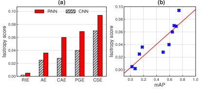
Figure 3: (a). The degree of isotropy of AWE for each model. (b) Correlation between the word discrimination performance measured by mAP and isotropy score (Pearson $r=0.89,p<0.001$).

To inspect the degree of isotropy of the AWE vector spaces, we use the IsoScore metric recently proposed by Rudman et al. (2022), which is—to the best of our knowledge—the only metric in the literature that is grounded on the mathematical definition of isotropy. The IsoScore metric operates on the covariance matrix of the embedding dimensions and returns values between 0 (minimally isotropic) and 1 (maximally isotropic). We quantify the degree of isotropy using IsoScore for each model type and show the result in Fig. 3(a). We observe that IsoScore returns values that are within the range [$0.002,0.095$], which indicates that embedding spaces for all models tend towards being minimally isotropic. However, the embeddings of untrained, randomly initialized encoders (RIE) tend to be extremely anisotropic (i.e., IsoScore values close to 0). This observation suggests that the anisotropic space does not “emerge” during the model training but rather that it is an inherent property of the encoder architecture. We are not aware of prior work in NLP that has studied the degree of isotropy in untrained NLP models to investigate whether anisotropic spaces are an emergent or inherent feature. In our case, training with a learning objective that encourages the model to separate word categories moves the representation space more towards utilizing more dimensions, therefore resulting in a higher degree of isotropy. Moreover, recurrent encoders tend to be more isotropic than their convolutional counterparts within the same learning objective.

Despite the tendency of all models to be anisotropic, we find a strong positive correlation between the degree of isotropy and the performance on word discrimination—see Fig. 3(b). That is, the more dimensions the model utilizes in the representation space, the better it performs on the intrinsic evaluation task.

5 Analysis 2: Word Discriminability

Ideally, AWE models should project exemplars of the same word category onto the same point in the embedding space. However, there are no strong constraints during training to encourage maximal separability between different word categories. In this analysis, we seek to answer two questions: (1) how well-separated are the word categories of the training samples? and (2) to what degree do lexical properties predict the discriminability of word categories?

5.1 Category Discriminability Index

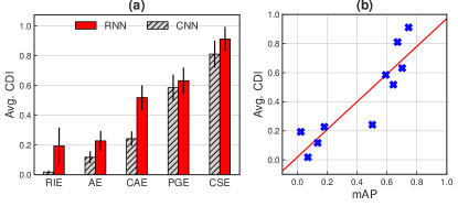
Figure 4: Averaged Category Discriminability Index (CDI) for each AWE model with error bars showing standard deviation over word categories. (b) Correlation between the word discrimination performance measured by mAP and averaged CDI (Pearson $r=0.90,p<0.001$).

In order to investigate the geometric density of each word category in the representation space, we need to measure within-category compactness and cross-category separability. Inspired by the exemplar discriminability index proposed in the neuroscience literature Nili et al. (2020), we define category discriminability index (CDI) as a metric that operates on within-category and cross-category distances. If we consider each lexical category in the training set as a set of its exemplar embeddings $\mathcal{C}=\{\mathbf{e}_{1},\dots,\mathbf{e}_{|\mathcal{C}|}\}$, CDI is defined for a single category $\mathcal{C}$ as

$$\text{CDI}(\mathcal{C})=\frac{1}{|\mathcal{C}|}\sum_{\forall\mathbf{e}_{i}\in\mathcal{C}}\\ \bigl{(}\sum_{\forall\mathbf{e}_{j}\sim\mathcal{C}|j\neq i}{d(\mathbf{e}_{i},\tilde{\mathbf{e}}_{j})}-d(\mathbf{e}_{i},\mathbf{e}_{j})\bigr{)}$$ (5)

where $d(.,.)$ is the cosine distance and $\mathbf{e}_{j}$ is a within-category sample while $\tilde{\mathbf{e}}_{j}$ is an embedding sampled from a different category. If we normalize the embeddings, CDI $\in[-1,1]$ with values closer to $1$ indicating higher word discriminability. We compute CDI for each word category in the training set and take the average over categories to estimate how well the categories are separated in the embedding space of each model type. The result of this analysis is shown in Fig. 4(a). For each learning objective, we observe that word discriminability is higher in the recurrent encoders compared to their convolutional counterparts. Besides that, the contrastive objective yields encoders with a higher word discriminability index regardless of the architecture type—recurrent vs. convolutional. Furthermore, we report a strong positive correlation between average CDI and the performance on the evaluation task—see Fig. 4(b), indicating that word discrimination performance on future, held-out samples can be predicted based on the CDI computed on the training samples.

5.2 Effect of Frequency and Distinctiveness

The CDI quantifies the separability and compactness for each lexical category in the representation space. Next, we aim to identify the factors that could make a lexical category compact and well-separable.

In this analysis, we study the effect of two lexical properties that could be quantified in a data-driven approach: word frequency and acoustic distinctiveness. Our initial hypothesis is that a word category with many training exemplars becomes more discriminable in the embedding space as the repeated exposure to samples of various degrees of variability should enable the model to learn compact and precise representation for categories with high frequency. Also, words that are acoustically distinct have fewer competitors in the perceptual space, thus they should be more separable than words with many phonological neighbours that sound similar. Therefore, we expect word acoustic distinctiveness (WAD) to positively correlate with CDI. In this analysis, we operationalize WAD using two metrics: word length (i.e., the number of phonemes) and phonological distinctiveness. Word length contributes to WAD since word formation in natural languages is a combinatorial process. That is, increasing the number of phonemes in a word-form decreases the likelihood of encountering a similarly sounding word-form which makes it less confusable. However, the word formation process is governed by language-specific phonotactic rules which makes some sound combinations more probable than others. To capture the probabilistic nature of sound sequences, we employ phonological information content (PIC), an information-theoretic metric that estimates WAD based on its phoneme-to-phoneme transition probabilities Meylan and Griffiths (2017). Given a word-form as a sequence of phonemes $\boldsymbol{\varphi}=(\varphi_{1},\dots,\varphi_{\tau})$, PIC is defined as

$$\text{PIC}(\boldsymbol{\varphi})=-\sum_{i=1}^{\tau}{\log p_{\boldsymbol{\theta}}(\varphi_{i}|\boldsymbol{\varphi}_{<i})}$$ (6)

where $p_{\boldsymbol{\theta}}$ is a probabilistic phoneme-level language model (PLM). We estimate $p_{\boldsymbol{\theta}}$ using a trigram PLM with the counts of the phonemes in the training word categories. Higher values of PIC indicate less probable phoneme sequences thus more distinct word-forms. Note that PIC is not length normalized and therefore shorter words tend to have lower PIC.

Next, we conduct a correlation analysis between word CDI and the three lexical predictors: frequency, length, and PIC. The result of this analysis is shown in Table 1. Surprisingly, our correlation analysis shows that lexical frequency is a poor predictor of CDI. Although in five out of eight models the frequency positively correlates with CDI, the correlation is rather weak. However, measures of acoustic distinctiveness have a stronger correlation with CDI compared to frequency, and the strength of the correlation is more noticeable in all decoding-based models—except the convolutional PGE—compared to contrastive models. We also find it surprising that PIC is not a better predictor of CDI than word length. However, it has been shown in a related work that autoencoder-based AWEs encode duration as an acoustic feature Matusevych et al. (2021). Taken together with our findings, this suggests that the models exploit and rely on acoustic word length as a feature to discriminate between the lexical categories. Arguably, word length is a more accessible feature to learn from the acoustic signal compared to structural phonological regularities in the training data.

Objective	Arch.	Frequency	Length	PIC
AE	cnn	-0.081†	0.315†	0.263†
	rnn	-0.087†	0.357†	0.306†
CAE	cnn	0.021	0.376†	0.274†
	rnn	0.077†	0.447†	0.359†
PGE	cnn	0.035	0.039*	-0.011
	rnn	-0.043*	0.325†	0.263†
CSE	cnn	0.131†	0.075†	0.031
	rnn	0.109†	0.100†	0.030

Table 1: Pearson correlation ($r$) between word category discriminability index (CDI) and three lexical properties: frequency, length, and phonological information content (PIC). Statistical significance is marked with * and † for $p<0.05$ and $p<0.001$, respectively.

6 Analysis 3: Network Representational Consistency

Suppose we train two instances of the same architecture and learning objective on the same training samples, but each with different random initializations. Do these two neural network instances exhibit differences in their representational geometries? In this section, we shed light on the representational discrepancies caused by different initializations. In other words, we are interested in quantifying the degree to which variability in the initial conditions affects the way two models separate the same set of speech samples.

6.1 Performance Stability

First, we quantify the effect of the initial weights on the evaluation task performance. To this end, we train six model instances—in identical setup but with different initializations—for each architecture and each learning objective, which yields 48 model instances in total (6 $\times$ 4 RNN runs and 6 $\times$ 4 CNN runs). We evaluate each model instance on the acoustic word discrimination task while observing the result variation per model type. The result of the performance stability analysis is shown in Table 2 in Appendix  D. We observe that all instances have converged and the performance is fairly stable across different runs.

6.2 Representational Discrepancies

Our previous performance stability analysis has demonstrated that different DNN instances exhibit only trivial quantitative differences. However, a stable performance on the evaluation task does not entail an identical representational geometry across different instances. That is, two network instances could have have an identical performance on the evaluation task while each having a distinct representational geometry. To closely investigate representational discrepancies between network instances, we employ the representational consistency (RC) analysis Mehrer et al. (2020), which is a neuroscience-inspired technique based on the representational similarity analysis (RSA) framework Kriegeskorte et al. (2008). For our analysis, we operationalize the RC using linear Centered Kernal Alignment (CKA) as a representational similarity measure of two views of the same input samples Kornblith et al. (2019). CKA abstracts away from the embeddings themselves and operates on pairwise distances between the sample representations. Concretely, given $K$ spoken-word samples $\boldsymbol{a}_{1}^{K}=\{\boldsymbol{a}_{1},\dots,\boldsymbol{a}_{K}\}$, we embed the samples using two encoder instances to obtain two different views of the samples $\mathbf{X}\in\mathbb{R}^{K\times D}$ and $\mathbf{Y}\in\mathbb{R}^{K\times D}$. Then, each view matrix is multiplied by a centering matrix $\mathbf{H}=\mathbf{I}_{K}-\mathbf{1}_{K}/K$ to make each column’s mean equal to zero and obtain centered second moment matrices as

$$\begin{split}&\mathbf{G}_{\mathbf{X}}=\mathbf{H}\mathbf{X}\mathbf{X}^{\top}\mathbf{H}^{\top}/D,\\ &\mathbf{G}_{\mathbf{Y}}=\mathbf{H}\mathbf{Y}\mathbf{Y}^{\top}\mathbf{H}^{\top}/D\end{split}$$ (7)

Then, the representational similarity of the two views is computed using CKA as

$$\text{CKA}(\mathbf{X},\mathbf{Y})=\frac{\langle\text{vec}(\mathbf{G}_{\mathbf{X}}),\text{vec}(\mathbf{G}_{\mathbf{Y}})\rangle}{||\mathbf{G}_{\mathbf{X}}||_{F}||\mathbf{G}_{\mathbf{Y}}||_{F}}$$ (8)

where $\text{vec}(.)$ is the vector-reshaped matrix, $\langle.,.\rangle$ is the inner product, and $||.||_{F}$ is the Frobenius norm to ensure that CKA $\in[0,1]$ where values close to 1 indicate that the two instances are highly consistent, while values close to 0 indicate low consistency.

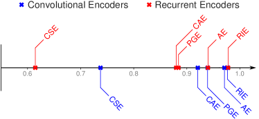
Figure 5: Network representational consistency (RC): (top) recurrent encoders and (bottom) convolutional encoders. Values closer to 1 indicates higher RC.

Using CKA, we conduct pairwise similarity analysis across all six instances which yields 15 comparisons for each model type. We report the mean of the resulting CKA values for each model type in Fig. 5. First, we observe that randomly initialized encoders (RIE) are highly consistent for both architectures ($\text{mean CKA}_{RIE/RNN}\approx\text{mean CKA}_{RIE/CNN}=0.98$). However, after training the encoder instances, convolutional networks are more consistent than their recurrent counterparts. Note that this behaviour cannot be attributed to a difference in the number of trainable parameters between the two architectures since they are comparable. Moreover, all decoding-based learning objectives return mean CKA values above 0.87, which indicates that their representational profiles are similar despite some noticeable differences especially among the recurrent encoders. The only exception to this trend are model instances trained with contrastive loss since they are significantly less consistent compared to the other learning objectives ($\text{mean CKA}_{CSE/RNN}=0.61$ and $\text{mean CKA}_{CSE/CNN}=0.74$). We emphasize that CKA is a second-order isomorphismic approach that operates on the similarity of the pairwise sample similarity matrices across different views. Therefore, the anisotropic nature of AWEs reported in §4 cannot explain their similarity-based representational profiles, and by implication, their representational consistency.

7 Discussion

Acoustic word embeddings (AWEs) are vector representations that encode the sound structure and acoustic-phonetic features of spoken words. AWEs are induced from actual acoustic realizations of speech, and therefore AWE models have to abstract away from non-linguistic dimensions of variability in speech signals (e.g., speaker characteristics, speech rate, recording conditions, etc). While analyzing the representational geometry of semantic word embeddings is a topic that has received a substantial attention in the NLP research community, the interpretability of AWEs remains an under-explored topic and we are aware of a few prior studies in this direction Matusevych et al. (2020b); Abdullah et al. (2021a, b). In this article, we made a number contributions in analyzing the representational geometry of AWEs and obtained research findings which we discuss and summarize in this section.

Learning objective affects the geometry more than architecture.   Our three analyses in this paper have shown that the learning objective shapes the representational geometry of the AWE encoders more than their underlying architectures. This finding suggests that recurrent and convolutional encoders exhibit similar inductive biases while the learning process is mainly guided by the loss function.

AWE models tend to be anisotropic.   Our analysis in §4 has shown that AWEs tend towards being minimally isotropic. However, this behavior is not an emergent property of the training process, but rather an inherent behavior of the neural network. Moreover, the degree of isotropy after training the model positively correlates with the acoustic word discrimination evaluation task. Since different models have different degree of isotropy and the representation space is not always uniform, we conclude that any comparison between different models based on absolute distance metrics such cosine distance will definitely lead to inaccurate observations.

Word distinctiveness, but not frequency, predicts category discriminability.   While word acoustic distinctiveness has been found in §5 to be a good predictor of the degree to which a word category is compact and well-separated in the embedding space, word frequency does not correlate with category discriminability. In retrospective, this finding should not be surprising as frequent words tend to have shorter lengths. Shorter words have more phonological neighbours that are perceptually similar in form and thus they are more confusable with other words. Future work could employ more sophisticated linear mixed effects models to analyse the interaction between different lexical properties such as frequency, phonological neighbourhood density, and word length and their effect on word category discriminability.

AWE models exhibit individual differences.   Although AWE model instances trained with different random initializations are stable with respect to the performance of the evaluation task, they exhibit individual differences in their representational profiles as shown in §6. However, the degree of the network representational consistency across different initializations depends on both the architecture and the learning objective. Contrastive objectives are less consistent than decoding-based objectives, while recurrent encoder are less consistent than their convolutional counterparts.

Contrastive models have distinct representational profiles.   In the analyses we presented in this paper, we observed that the contrastive encoders behave differently than other encoders trained with non-contrastive losses. For example, word distinctiveness has been found to be a weak predictor of category discriminability in the embedding spaces of the contrastive encoders. Recall that our contrastive encoders have a stronger constraint in grouping exemplars of the same category closer in the embedding space guided by the margin hyperparameter, while decoding-based model lack this constraint. We hypothesize that this constraint forces the models to emphasize the separability of the lexical categories in the embedding space. Therefore, a stronger constraint seems to make contrastive encoders different compared to other learning objectives and different instances of the same contrastive encoder are less consistent in their representational geometry.

8 Conclusion

In this paper, we have taken a closer, analytical look at the representational geometry of acoustic word embeddings (AWEs) from three different, but complementary perspectives: (1) embedding space uniformity, (2) word discriminability, and (3) network representational consistency. We have shown that the representational spaces of AWEs tend towards being minimally isotropic, or in other words, they utilize only a few dimensions of the embedding space. Another finding was that most AWE models rely on word length as a feature to discriminate between lexical categories since the word discriminability index positively correlates with the number of phonemes in a word. Furthermore, our representational consistency analysis have shown that AWE models exhibit individual differences in their representational profiles, with the contrastive encoders being the most inconsistent across different random initializations.

Even though we focused on acoustic word embeddings in this paper, our analytic methodology can also be employed for the interpretability of self-supervised speech representation models such as contrastive predictive coding Oord et al. (2018) and wav2vec Schneider et al. (2019). Also, the emergent representations of sublexical units such phonemes and syllables in speech neural networks can be analyzed using the our proposed methodology in this paper.

9 Acknowledgements

The authors would like to thank the anonymous reviewers for their encouraging feedback and insightful comments on the paper. We express our heartfelt thanks to Miriam Schulz for proofreading the paper. This research is funded by the Deutsche Forschungsgemeinschaft (DFG, German Research Foundation), Project-ID 232722074 – SFB 1102.

Appendices

Appendix A AWE Models

See Fig. 6 for a visual illustration of the different learning objectives in our paper.

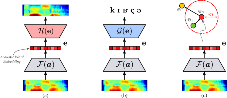
Figure 6: A visual illustration of the different learning objectives for training AWE encoders: (a) correspondence auto-encoder (CAE): a sequence-to-sequence network with an acoustic decoder, (b) phonologically guided encoder (PGE): a sequence-to-sequence network with a phonological decoder, and (c) contrastive siamese encoder (CSE): a contrastive network trained via triplet margin loss. After training the model, only the encoder component of the model $\mathcal{F}$ is used to produce AWEs.

Appendix B Intrinsic Evaluation

The results of the intrinsic evaluation—same-different word discrimination task quantified by the mAP metric—is shown in Fig. 7. Note that the CAE model is pre-trained as autoencoder for 10 epochs, following prior work Kamper (2019).

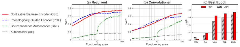
Figure 7: Evaluation on the same-different acoustic word discrimination task quantified by the word discrimination task and the mAP metric: Learning curves of 100 training epochs for (a) the recurrent encoder and (b) convolutional encoders. (c) mAP of the best epoch.

Appendix C Randomly Initialized CNN Encoder

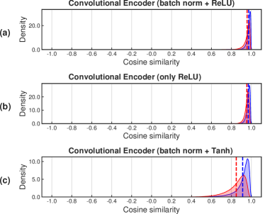
Figure 8: Cosine similarity distributions across three different variants of convolutional encoders: (a) convolutional layers with batch normalization and ReLU non-linearity, (b) convolutional layers with ReLU non-linearity but without batch normalization, and (3) convolutional layers with batch normalization and Tanh non-linearity.

To further investigate the minimally isotropic behavior and the near 1 values of cosine similarities of the untrained, randomly initialized convolutional encoder reported in §4, we examine the potential contribution of two factors to this observation; batch normalization (BN) and the activation function of the convolutional layers. The result of this analysis is depicted in Fig. 8. We observe that removing the BN layer has no effect on the distributions of cosine similarities as they remain almost identical to the encoder that has a BN layer—see Fig. 8(b). However, changing the activation function from the unbounded ReLU to the bounded Tanh in the convolutional layers makes the distributions of cosine similarities move towards zero mean, even though they remain closer to 1 than 0. Therefore, this behavior seems to be related to the inner dynamics of the convolutional operation and gets amplified where the activation function in the convolutional layers are unbounded. Nevertheless, identifying the source of this behavior requires further investigation with different activation functions and a controlled ablation study.

Appendix D Performance Stability across Different Runs

For the analysis in §6, we have trained six neural network instances for each encoder type using the same training samples to investigate the performance stability and representational consistency of training runs that differ in their random seeds. A summary statistics for the performance on the evaluation task measured by the mAP metric is shown in Table  2. One can observe only trivial differences on the evaluation tasks. Therefore, we conclude that the performance of different training runs is stable and our findings on the network representational consistency reported in §6 cannot be explained by quantitative differences, but rather by representational discrepancies due to disagreement in the geometric arrangement of the speech samples in the embedding space.

Appendix E Qualitative Analysis

To further inspect the representation space and its neighborhood structure, we conduct a qualitative analysis by querying the representation space with a few word samples. In this analysis, we compute word category centroids by averaging the word embeddings of the training samples, then we use a word centroid as a query and obtain the top-10 ranked nearest neighbors. The result of this analysis is shown in Fig. 3. For the majority of the examples in Fig. 3, we observe that there is a strong word onset bias where the most similar words are those that begin with a similar sounding prefix as the query word.

Objective	Arch.	mean	max	min	std
AE	cnn	0.137	0.141	0.133	0.0026
	rnn	0.183	0.186	0.179	0.0024
CAE	cnn	0.505	0.510	0.500	0.0040
	rnn	0.646	0.650	0.643	0.0029
PGE	cnn	0.595	0.599	0.592	0.0033
	rnn	0.704	0.710	0.687	0.1000
CSE	cnn	0.676	0.680	0.674	0.0023
	rnn	0.742	0.745	0.739	0.0027

Table 2: mAP statistics across six different runs for each model type.

Query ($\downarrow$)	Convolutional Encoders (CNN)				Recurrent Encoders (RNN)
	AE	CAE	PGE	CSE	AE	CAE	PGE	CSE
mentioned	mention	mention	mention	mention	mention	mention	mention	mention
	wretched	mansion	mansion	mansion	wretched	mansion	mansion	mansion
	nation	motion	legends	merchant	nation	merchant	merchant	merchant
	midst	merchant	management	mission	merchant	motion	legends	mission
	merchants	making	merchants	mental	motion	nation	mountain	pinching
	motion	wilson	magic	vincent	merchants	making	merchants	massive
	merchant	nation	matrons	pinching	midst	vincent	mission	mental
	message	midst	mission	medicine	milking	nineteen	magician	transient
	regiment	missing	merchant	crouching	winter	nature	motion	motion
	winter	nature	magician	midst	vessel	rachel	wretched	hudson
intellectual	individual	introduction	intellect	intellect	individual	individual	individual	introduction
	interesting	individual	individual	adjoining	interesting	introduction	intelligence	individual
	indifferent	interrupted	introduction	recollection	neglected	uncomfortable	introduction	immature
	newton	indifference	intelligent	delightful	petition	intelligent	intellect	objection
	institution	attraction	encouragement	individual	magician	intelligence	uncomfortable	implacable
	departure	intellect	interrupted	employing	hokosa	interesting	intelligent	delightful
	imitation	immature	intelligence	impetuous	compassion	invisible	interpretation	theatrical
	hokosa	indifferent	indifferently	employed	departure	interrupted	industrial	thoughtful
	encountered	encouragingly	unconditional	natural	convention	imperfectly	incapable	industrial
	neglected	implacable	impetuous	accumulated	consulted	incredible	insensible	election
maker	labor	naked	naked	baker	labor	nature	baker	liquor
	liquor	natured	liquor	naked	nature	local	nature	negro
	labored	nature	natured	negro	walker	naked	liquor	eaten
	labour	local	nature	liquor	local	labour	labour	baker
	wicker	labour	baker	local	naked	labor	labor	nature
	leaping	major	major	native	labour	major	major	labor
	lifted	labor	negro	nature	rachel	natured	negro	naked
	walker	native	native	major	liquor	baker	neighbors	newspaper
	local	making	wicker	matrons	labored	liquor	vapor	mink
	nature	navy	labor	vigor	leaping	negro	labors	vigour
profession	position	procession	procession	professor	position	procession	procession	professor
	proceed	professor	professor	sufficient	professors	possession	proportion	procession
	positions	position	position	procession	possessions	position	perfection	perfection
	physician	possession	petition	professors	proceeded	professor	possession	sufficient
	proceeded	professors	pushing	efficiency	physician	possessions	protection	proposition
	possessed	pushing	professors	efficient	condition	permission	proportions	proportion
	prison	perfection	possession	petition	procession	discussion	position	production
	possessions	positions	physician	prevent	presumption	positions	possessions	petition
	perfect	discussion	positions	position	protested	commission	professor	compassion
	discussion	preferred	precious	physician	proceed	physician	petition	pushing
seized	ceased	ceased	ceased	thieves	ceased	ceased	ceased	thieves
	freedom	season	seizing	ceased	faded	feasts	thieves	ceased
	seated	thieves	season	season	cities	scenes	saves	fuse
	faded	saves	thieves	feast	singing	thieves	seats	jesus
	singing	seems	saves	seizing	scenes	saves	seems	spheres
	scenes	scenes	ceasing	feared	feeding	seems	scenes	feels
	season	ceasing	seems	ceasing	season	feast	seemed	cities
	cities	saints	feast	saves	sweetest	saints	feast	season
	field	feast	seats	species	seated	faced	saved	seats
	seeming	sins	seemed	speed	saying	seemed	seizing	scenes
experiments	experiment	experiment	experiment	experiment	experiment	experiment	experiment	experiment
	experience	experienced	experience	experienced	experienced	experienced	experienced	attendants
	experienced	experience	experienced	garments	experience	experience	experience	extremities
	experiences	experiences	experiences	extermination	extinguished	experiences	experiences	islands
	extinguished	extremities	expense	expense	experiences	exposed	expressions	experienced
	exchange	established	embarrassment	experience	expected	extremities	extermination	prominence
	extremities	extraordinary	expanse	aramis	exchange	expense	extremities	edmunds
	expressions	extinguished	extraordinary	disturbance	expressions	expanse	extremity	instruments
	extremely	extremity	extremities	examined	extremities	extinguished	expression	attendance
	extremity	expanse	expressions	vanished	extent	exclusion	expensive	commons

Table 3: Top-10 nearest word embedding centroids for a word sample.

References

- Abdullah et al. (2021a) Badr M. Abdullah, Marius Mosbach, Iuliia Zaitova, Bernd Mobius, and Dietrich Klakow. 2021a. Do acoustic word embeddings capture phonological similarity? An empirical study. In Interspeech.
- Abdullah et al. (2021b) Badr M. Abdullah, Iuliia Zaitova, Tania Avgustinova, Bernd Möbius, and Dietrich Klakow. 2021b. How familiar does that sound? cross-lingual representational similarity analysis of acoustic word embeddings. In Proceedings of the Fourth BlackboxNLP Workshop on Analyzing and Interpreting Neural Networks for NLP, pages 407–419, Punta Cana, Dominican Republic. Association for Computational Linguistics.
- Algayres et al. (2020) Robin Algayres, Mohamed Salah Zaiem, Benoît Sagot, and Emmanuel Dupoux. 2020. Evaluating the Reliability of Acoustic Speech Embeddings. In Proc. Interspeech.
- Bengio and Heigold (2014) Samy Bengio and Georg Heigold. 2014. Word embeddings for speech recognition. In Proc. Interspeech.
- Bird (2021) Steven Bird. 2021. Sparse transcription. Computational Linguistics, 46(4):713–744.
- Cai et al. (2020) Xingyu Cai, Jiaji Huang, Yuchen Bian, and Kenneth Church. 2020. Isotropy in the contextual embedding space: Clusters and manifolds. In International Conference on Learning Representations.
- Carlin et al. (2011) Michael A Carlin, Samuel Thomas, Aren Jansen, and Hynek Hermansky. 2011. Rapid evaluation of speech representations for spoken term discovery. In Proc. Interspeech.
- Ethayarajh (2019) Kawin Ethayarajh. 2019. How contextual are contextualized word representations? Comparing the geometry of BERT, ELMo, and GPT-2 embeddings. In Proceedings of the 2019 Conference on Empirical Methods in Natural Language Processing and the 9th International Joint Conference on Natural Language Processing (EMNLP-IJCNLP), pages 55–65, Hong Kong, China. Association for Computational Linguistics.
- Grand et al. (2022) Gabriel Grand, Idan Asher Blank, Francisco Pereira, and Evelina Fedorenko. 2022. Semantic projection recovers rich human knowledge of multiple object features from word embeddings. Nature Human Behaviour, pages 1–13.
- Jacobs et al. (2021) Christiaan Jacobs, Yevgen Matusevych, and Herman Kamper. 2021. Acoustic word embeddings for zero-resource languages using self-supervised contrastive learning and multilingual adaptation. In 2021 IEEE Spoken Language Technology Workshop (SLT), pages 919–926. IEEE.
- Jansen and Durme (2012) Aren Jansen and Benjamin Van Durme. 2012. Indexing raw acoustic features for scalable zero resource search. In Proc. Interspeech.
- Johnson et al. (2017) Jeff Johnson, Matthijs Douze, and Hervé Jégou. 2017. Billion-scale similarity search with GPUs. IEEE Transactions on Big Data.
- Jurafsky (2003) Dan Jurafsky. 2003. Probabilistic modeling in psycholinguistics: Linguistic comprehension and production. Probabilistic linguistics, 21.
- Kamper et al. (2016a) H. Kamper, W. Wang, and Karen Livescu. 2016a. Deep convolutional acoustic word embeddings using word-pair side information. In Proc. ICASSP.
- Kamper (2019) Herman Kamper. 2019. Truly unsupervised acoustic word embeddings using weak top-down constraints in encoder-decoder models. In Proc. ICASSP.
- Kamper et al. (2015) Herman Kamper, Micha Elsner, Aren Jansen, and Sharon Goldwater. 2015. Unsupervised neural network based feature extraction using weak top-down constraints. In Proc. ICASSP.
- Kamper et al. (2016b) Herman Kamper, Weiran Wang, and Karen Livescu. 2016b. Deep convolutional acoustic word embeddings using word-pair side information. In Proc. ICASSP.
- Kingma and Ba (2015) Diederik P. Kingma and Jimmy Ba. 2015. Adam: A method for stochastic optimization. In Proc. ICLR.
- Kornblith et al. (2019) Simon Kornblith, Mohammad Norouzi, Honglak Lee, and Geoffrey Hinton. 2019. Similarity of neural network representations revisited. In International Conference on Machine Learning, pages 3519–3529. PMLR.
- Kriegeskorte et al. (2008) Nikolaus Kriegeskorte, Marieke Mur, and Peter A Bandettini. 2008. Representational similarity analysis-connecting the branches of systems neuroscience. Frontiers in systems neuroscience, 2:4.
- Levin et al. (2013) Keith Levin, Katharine Henry, Aren Jansen, and Karen Livescu. 2013. Fixed-dimensional acoustic embeddings of variable-length segments in low-resource settings. In IEEE Workshop on Automatic Speech Recognition and Understanding (ASRU).
- Matusevych et al. (2020a) Yevgen Matusevych, Herman Kamper, and Sharon Goldwater. 2020a. Analyzing autoencoder-based acoustic word embeddings. In BAICS Workshop ICLR.
- Matusevych et al. (2020b) Yevgen Matusevych, Herman Kamper, and Sharon Goldwater. 2020b. Analyzing autoencoder-based acoustic word embeddings. In Bridging AI and Cognitive Science Workshop, ICLR 2020.
- Matusevych et al. (2021) Yevgen Matusevych, Herman Kamper, Thomas Schatz, Naomi Feldman, and Sharon Goldwater. 2021. A phonetic model of non-native spoken word processing. In Proceedings of the 16th Conference of the European Chapter of the Association for Computational Linguistics: Main Volume, pages 1480–1490, Online. Association for Computational Linguistics.
- McAuliffe et al. (2017) Michael McAuliffe, Michaela Socolof, Sarah Mihuc, Michael Wagner, and Morgan Sonderegger. 2017. Montreal Forced Aligner: Trainable text-speech alignment using Kaldi. In Interspeech.
- McInnes et al. (2018) Leland McInnes, John Healy, Nathaniel Saul, and Lukas Großberger. 2018. Umap: Uniform manifold approximation and projection. Journal of Open Source Software, 3(29):861.
- Mehrer et al. (2020) Johannes Mehrer, Courtney J Spoerer, Nikolaus Kriegeskorte, and Tim C Kietzmann. 2020. Individual differences among deep neural network models. Nature communications, 11(1):1–12.
- Metze et al. (2013) Florian Metze, Xavier Anguera, Etienne Barnard, Marelie Davel, and Guillaume Gravier. 2013. The spoken web search task at MediaEval 2012. In Proc. ICASSP.
- Meylan and Griffiths (2017) Stephan C. Meylan and Thomas L. Griffiths. 2017. Word forms - not just their lengths- are optimized for efficient communication. ArXiv, abs/1703.01694.
- Mikolov et al. (2013) Tomas Mikolov, Ilya Sutskever, Kai Chen, Greg S Corrado, and Jeff Dean. 2013. Distributed representations of words and phrases and their compositionality. Advances in neural information processing systems, 26.
- Mimno and Thompson (2017) David Mimno and Laure Thompson. 2017. The strange geometry of skip-gram with negative sampling. In Proceedings of the 2017 Conference on Empirical Methods in Natural Language Processing, pages 2873–2878, Copenhagen, Denmark. Association for Computational Linguistics.
- Mu and Viswanath (2018) Jiaqi Mu and Pramod Viswanath. 2018. All-but-the-top: Simple and effective postprocessing for word representations. In International Conference on Learning Representations.
- Myers et al. (1980) Cory Myers, Lawrence Rabiner, and Andrew Rosenberg. 1980. An investigation of the use of dynamic time warping for word spotting and connected speech recognition. In ICASSP’80. IEEE International Conference on Acoustics, Speech, and Signal Processing, volume 5, pages 173–177. IEEE.
- Nematzadeh et al. (2017) Aida Nematzadeh, Stephan C. Meylan, and Thomas L. Griffiths. 2017. Evaluating vector-space models of word representation, or, the unreasonable effectiveness of counting words near other words. Cognitive Science.
- Nili et al. (2020) Hamed Nili, Alexander Walther, Arjen Alink, and Nikolaus Kriegeskorte. 2020. Inferring exemplar discriminability in brain representations. Plos one, 15(6):e0232551.
- Oord et al. (2018) Aaron van den Oord, Yazhe Li, and Oriol Vinyals. 2018. Representation learning with contrastive predictive coding. arXiv preprint arXiv:1807.03748.
- Panayotov et al. (2015) Vassil Panayotov, Guoguo Chen, Daniel Povey, and Sanjeev Khudanpur. 2015. Librispeech: an asr corpus based on public domain audio books. In 2015 IEEE international conference on acoustics, speech and signal processing (ICASSP), pages 5206–5210. IEEE.
- Paszke et al. (2019) Adam Paszke, Sam Gross, Francisco Massa, Adam Lerer, James Bradbury, Gregory Chanan, Trevor Killeen, Zeming Lin, Natalia Gimelshein, Luca Antiga, et al. 2019. Pytorch: An imperative style, high-performance deep learning library. In Proc. NeuRIPS.
- Pennington et al. (2014) Jeffrey Pennington, Richard Socher, and Christopher D Manning. 2014. Glove: Global vectors for word representation. In Proceedings of the 2014 conference on empirical methods in natural language processing (EMNLP), pages 1532–1543.
- Pereira et al. (2016) Francisco Pereira, Samuel Gershman, Samuel Ritter, and Matthew Botvinick. 2016. A comparative evaluation of off-the-shelf distributed semantic representations for modelling behavioural data. Cognitive neuropsychology, 33(3-4):175–190.
- Rohlicek (1995) Jan Robin Rohlicek. 1995. Word spotting. In Modern Methods of Speech Processing, pages 123–157. Springer.
- Rudman et al. (2022) William Rudman, Nate Gillman, Taylor Rayne, and Carsten Eickhoff. 2022. IsoScore: Measuring the uniformity of embedding space utilization. In Findings of the Association for Computational Linguistics: ACL 2022, pages 3325–3339, Dublin, Ireland. Association for Computational Linguistics.
- San et al. (2021) Nay San, Martijn Bartelds, Mitchell Browne, Lily Clifford, Fiona Gibson, John Mansfield, David Nash, Jane Simpson, Myfany Turpin, Maria Vollmer, et al. 2021. Leveraging pre-trained representations to improve access to untranscribed speech from endangered languages. In 2021 IEEE Automatic Speech Recognition and Understanding Workshop (ASRU), pages 1094–1101. IEEE.
- Schneider et al. (2019) Steffen Schneider, Alexei Baevski, Ronan Collobert, and Michael Auli. 2019. wav2vec: Unsupervised pre-training for speech recognition. arXiv preprint arXiv:1904.05862.
- Settle et al. (2019) Shane Settle, Kartik Audhkhasi, Karen Livescu, and Michael Picheny. 2019. Acoustically grounded word embeddings for improved acoustics-to-word speech recognition. In Proc. ICASSP.
- Settle and Livescu (2016a) Shane Settle and Karen Livescu. 2016a. Discriminative acoustic word embeddings: Recurrent neural network-based approaches. In IEEE Spoken Language Technology Workshop (SLT).
- Settle and Livescu (2016b) Shane Settle and Karen Livescu. 2016b. Discriminative acoustic word embeddings: Recurrent neural network-based approaches. In Proc. IEEE Spoken Language Technology Workshop (SLT).
- Strunk et al. (2014) Jan Strunk, Florian Schiel, and Frank Seifart. 2014. Untrained forced alignment of transcriptions and audio for language documentation corpora using webmaus. In Proceedings of the Ninth International Conference on Language Resources and Evaluation (LREC’14), pages 3940–3947.
- Zhang and Glass (2009) Yaodong Zhang and James R Glass. 2009. Unsupervised spoken keyword spotting via segmental DTW on Gaussian posteriorgrams. In IEEE Workshop on Automatic Speech Recognition & Understanding (ASRU).