Dynamic online prediction model and its application to automobile claim frequency data

Abstract

Prediction modelling of claim frequency is an important task for pricing and risk management in non-life insurance and needed to be updated frequently with the changes in the insured population, regulatory legislation and technology. Existing methods are either done in an ad hoc fashion, such as parametric model calibration, or less so for the purpose of prediction. In this paper, we develop a Dynamic Poisson state space (DPSS) model which can continuously update the parameters whenever new claim information becomes available. DPSS model allows for both time-varying and time-invariant coefficients. To account for smoothness trends of time-varying coefficients over time, smoothing splines are used to model time-varying coefficients. The smoothing parameters are objectively chosen by maximum likelihood. The model is updated using batch data accumulated at pre-specified time intervals, which allows for a better approximation of the underlying Poisson density function. The proposed method can be also extended to the distributional assumption of zero-inflated Poisson and negative binomial. In the simulation, we show that the new model has significantly higher prediction accuracy compared to existing methods. We apply this methodology to a real-world automobile insurance claim data set in China over a period of six years and demonstrate its superiority by comparing it with the results of competing models from the literature.

Keywords: state space model; dynamic prediction; time-varying; claim frequency data

Article History: March 1, 2024

1 Introduction

Determining future numbers of claims is one of the main tasks that actuaries perform in the insurance industry, especially in the insurance ratemaking process. A well-performed prediction model should maintain its accuracy over time. Most existing prediction methods in actuarial science can be featured by static prediction models, such as generalized linear models and their extensions (Klein et al., 2015, Lee, 2021, Lambert, 1992, Yip and Yau, 2005). Many insurance examples have shown that the performance of static prediction models easily tends to worsen over time. This is usually due to changes over time in the populations of insured groups, irregular claims behaviors, legislative change, or technological progress (Zhu et al., 2011, Chang and Shi, 2020, Dong and Chan, 2013, Henckaerts and Antonio, 2022). Some methods have been proposed to address this issue, such as model refitting and recalibration. However, these methods are often done in an ad hoc fashion. In this paper, we propose a dynamic prediction model in which the parameter estimates and prediction of future numbers of claims can be sequentially updated over time. It is well suited for massive data streams in which the data-generating process is itself changing over time. Furthermore, it is an online implementation that allows rapid updating of model parameters as new claim data arrive.

The frequently used methodology of predicting future claim frequency based on multi-year insurance claim data is the credibility theory, in which the time dependence structure is modelled by random effects (Denuit and Lu, 2021, Lee et al., 2020). Recently, several credibility models with dynamic random effects have been adapted to a longitudinal context to conduct experience ratemaking, where the risk of a policyholder is governed by an individual process of unobserved heterogeneity (Taylor, 2018, Pinquet, 2020, Ahn et al., 2022, Lu, 2018). However, it remains some challenges in the insurance dynamic ratemaking literature. Firstly, the fact that the prediction models mentioned above have to rely on longitudinal data is a very strong limitation, as the changing population of insured groups every year makes it difficult for insurers to collect and collate individual policies into longitudinal data. These approaches will result in the reduction of massive claim information due to the exclusion of early surrendered and non-renewed policies. Secondly, insures will be plagued by the computational burden for predicting future premiums in the dynamic random effect models as the Bayesian credibility premium typically lacks tractability (Li et al., 2021). Thirdly, while the existing methods allow random effects to be varied over time (Pinquet, 2020), they are still static models where the regression parameters are assumed fixed throughout the data, which will cause the model’s parameter estimates to track the parameters poorly when the effect of risk factors is subject to variation over time (Chang and Shi, 2020). Moreover, these models are too restrictive for capturing complicated nonlinear relationships between response variables and covariates over time. These motivate us to propose a relatively simple prediction model structure for numbers of claim as functions of several important rating factors, but allow the model parameters to vary with time and capture the complicated nonlinear effects of time. This leads our study of varying-coefficient models (Hastie and Tibshirani, 1993, Fan and Zhang, 2008). Specifically, for this context, since the varying-coefficient models are readily interpretable, we can provide a standard interface between the statistical model and the insurance ratemaking mechanism by reporting the fitted individual regression parameters. However, the vary-coefficient models in statistics mainly focus on estimation and statistical inference rather than future prediction, as both kernel and spline-based estimators are not suitable for prediction.

State space models are powerful tools in modelling dynamic systems and have been developed for both Gaussian and non-Gaussian response, with its application in biology (Bhattacharjee et al., 2018), medicine (Jiang et al., 2021), epidemiology (O’Neill, 2002) and insurance (Lai and Sun, 2012, Ahn et al., 2022, Fung et al., 2017). In this method, the dynamic system is modelled over time by a set of latent parameters that determine the changing distribution of observed data. The hierarchical model structure allows for both making statistical inferences and predicting future outcomes, taking into account the observed past trajectory. For Gaussian distribution, there is a closed-form solution for estimating the parameters. For the non-Gaussian distribution, such as the claim count data in our motivating example, the solution often relies on complicated numerical integration Normal approximations like the Laplace approximation are commonly used (Lewis and Raftery, 1997a) for computational convenience.

In insurance applications, the system characteristics change slowly over time and might be subject to changes in insurance regulatory legislation. A commonly used method is to model the parameter of interest as a smooth function over time, for example, smoothing spline. Wahba (1978) and Wahba (1983) show that the estimation of a smoothing spline for a Gaussian outcome is equivalent to the posterior estimate of a Gaussian stochastic process. Gu (1992) shows that it also holds for Non-Gaussian outcomes with the Laplace approximation. Wecker and Ansley (1983) show how to fit smoothing splines using the state space model formulation. Recently, Jiang et al. (2021) discuss the dynamic binary classification problem based on state space model for clinical decision marking. However, this approach is not suitable for insurance ratemaking as the claim count data usually exhibits the over-dispersion features with an excess of zeros. Motivated by modelling the claim frequency of automobile insurance based on the multi-year claim data, we propose a Dynamic Poisson state space (DPSS) model in which time-varying coefficients modelled by the state equations. The underlying distribution assumption of Poisson distribution can be extended to negative-binomial distribution and zero-inflated Poisson distribution to capture the zero-inflated and over-dispersion features of claim count data. Similar to the traditional Poisson model, the DPSS model regards the number of claims as the response variable, and employs a log-link function to connect the response variable to the covariates. In contrast to the traditional Poisson model, the time-varying coefficients in the DPSS model are modelled using smoothing splines, similar to Wecker and Ansley (1983). The smoothing parameters in the proposed models are estimated via maximum likelihood on the training data. The K-steps ahead prediction for claim frequency is based on an algorithm similar to Kalman filter, which allows for the smoothing parameters, model coefficients, and also prediction to be updated dynamically when new claim data becomes available. The advantage of the proposed method is that the updates only need to be computed on the additional observations when new claim data becomes available, whereas it is only updated as each new observation becomes available in the standard state space model. Since the filtering step often involves a Laplace approximation for count outcomes, updating one observation at a time will lead to large cumulative approximation errors. In addition, it is often not feasible or desirable to update the model one data at a time in applications. Consequently, we propose to update the model at pre-specified fixed time intervals when a batch of claims data becomes available.

Although there has been a branch of actuarial science literature on state space models in mortality forecasting (Chang and Shi, 2020) and non-life insurance ratemaking (Ahn et al., 2022), there are few studies to discuss how to embed state space models into varying-coefficient models for future prediction. To the best of our knowledge, this is the first study of the dynamic prediction model under a claim-frequency-modelling framework. By adopting the time-varying coefficient model with tools of state-space modelling, our DPSS model significantly fills the gap in dynamic claim frequency modelling and forecasting. The computational efficiency of our proposed method enables it to be implemented for online monitoring. It should also be noted that while the proposed method is designed for predicting claim frequency, it can be easily extended to the prediction of claim severity and pure premium by assuming the response follows other continuous heavy-tailed distribution, i.e, gamma distribution, or semi-continuous distribution, i.e., compound Poisson distribution or Tweedie distribution (Jørgensen and Smyth, 1994).

To demonstrate the application of the proposed method, we analyze a novel Chinese data set on automobile insurance, followed over the years from 2010 to 2015 with claim history and self-reported risk characteristics of approximately 440,000 policies. Our goal is to start from a ratemaking model with static parameters and to develop a dynamic mechanism that adjusts the baseline price of rating factors utilizing the introduction of time-varying coefficients. Strong empirical evidence suggests this model’s superiority over the static prediction model. Moreover, we present empirical evidence of the time-varying effect, including expo, carusage, carseats, carorigin, coverage, gender, ptype and svolume as estimated by the DPSS model . The decreasing trend after the year 2012 can be observed for the estimated regression coefficients of most of the rating factors. We argue that these dynamic patterns can be caused by the changing automobile regulatory policy in China as regulators tighten insurers’ rights to set their insurance premiums, aiming to promote uniform automobile premium rate standards. Therefore, identifying and understanding the time-varying effects and the causes of these effects is critical for theoretical research and actuarial ratemaking practice.

The structure of this paper is as follows. In Section 2 we first provide a summary of the partial varying coefficient model and state space model and then introduce a new class of Dynamic Poisson state space models. Estimation and prediction procedure are discussed in Section 3. The advantages of DPSS model compared to several established methods in the insurance ratemaking literature are illustrated by a simulation study in Section 4. To illustrate its practical use, in Section 5, we conduct an analysis of the DPSS model fitted to a Chinese automobile insurance data set over most six years periods. Section 6 gives some conclusions and future possible extensions.

2 Methodology

2.1 Partial varying coefficient model

Classical generalized linear models are not feasible to capture the time-varying effects of covariates. A more sophisticated model is varying-coefficient models (Hastie and Tibshirani, 1993). They allow the regression coefficients to vary in a smooth way with another variable (for example time). Let $(y_{i},\bm{x}_{i},t_{i})$ for $i=1,\cdots,n$ be the observed data for each subject $i$ at observed time $t_{i}$, where $0\leq t_{1}<t_{2}<\cdots<t_{n}\leq 1$, $\bm{x}_{i}=(x_{i1},\cdots,x_{iq})^{T}$ denotes a $q$-dimensional vector of covariates, and $y_{i}$ is the insured claim count (the number of claims). We propose the following model for $y_{i}$ in which $\lambda_{i}$ is the intensity (expected claim frequency), that is,

$$y_{i}\sim\text{Poisson}(\lambda_{i}),$$

with

$$\log\left({{\lambda}_{i}}\right) =\beta_{0}(t_{i})+\sum_{j=1}^{q_{1}}\beta_{j}(t_{i})x_{ij}+\sum_{k=1}^{q_{2}}\alpha_{k}x_{i,q_{1}+k}$$

$$=\bm{x}_{i1}^{T}\bm{\beta}\left({{t}_{i}}\right)+\bm{x}_{i2}^{T}\bm{\alpha},$$ (2.1)

where $\bm{x}_{i1}=(1,x_{i1},\cdots,x_{iq_{1}})^{T}$ and $\bm{x}_{i2}=(x_{i,q_{1}+1},\cdots,x_{i,q})^{T}$ are the covariates with varying coefficients $\bm{\beta}(t)=(\beta_{0}(t),\beta_{1}(t),\cdots,\beta_{q_{1}}(t))^{T}$ and with time-invariant coefficients $\bm{\alpha}=(\alpha_{1},\cdots,\alpha_{q_{2}})^{T}$ respectively, and $q_{1}+q_{2}=q$. The varying-coefficient regression models have got lot of researches in statistics literature since proposed by Hastie and Tibshirani (1993); see Fan and Zhang (2008), Park et al. (2015) for a comprehensive review. However, most existing literatures are all focused on the problem of estimation and statistical inference rather than prediction.

Remark 1.

In the context of automobile insurance ratemaking, we usually assumes that the number of claims, $Y_{i}$, is Poisson distribution with mean $\mathbb{E}(Y_{i})=w_{i}\lambda_{i}$, where $w_{i}$ is risk exposure and $\lambda_{i}=\exp(\bm{x}_{i}^{T}\bm{\beta})$. Then we have $\log\mathbb{E}(Y_{i})=\log(w_{i})+\bm{x}_{i}^{T}\bm{\beta}$, in which $\log(w_{i})$ can be viewed as covariate with fixed coefficient 1. In (2.1) we treat $\log(w_{i})$ as covariates with unknown coefficients. Thus, the traditional Poisson regression model can be regarded as a special case of (2.1).

Remark 2.

Although Poisson distribution is a natural candidate for modelling count data, it is commonly found that the number of zeros in insurance claim data exceeds the number of zeros predicted from the Poisson model. To model the excessive zeros phenomenon in claim count distribution, the zero-inflated Poisson (ZIP) model proposed by Lambert (1992) is usually used to fit automobile insurance claims (Yip and Yau, 2005). To deal with overdispersion, where the assumption of equal expectation and variance inherent in the Poisson distribution has to be replaced by variances exceeding the expectation, the negative-binomial distribution provides a convenient framework extending the Poisson distribution by a second parameter determining the scale of the distribution, see for example Hilbe (2011). Using the well-known negative-binomial (NB) and zero-inflated Poisson (ZIP), we further extend the Dynamic Poisson state space model (DPSS) to Dynamic negative-binomial state space model (DNBSS) and Dynamic zero-inflated Poisson state space model (DZIPSS). The model specifications and estimation procedures can be found in appendix A and B for more details.

The parameters can be estimated through maximizing the following penalized log-likelihood function:

$${{L}_{c}}\left(\bm{\alpha},\bm{\beta}(t);\bm{y}\right) =\sum\limits_{i=1}^{n}{\left\{{{y}_{i}}\left[\bm{x}_{i1}^{T}\bm{\beta}\left({{t}}\right)+\bm{x}_{i2}^{T}\bm{\alpha}\right]-\exp\left[\bm{x}_{i1}^{T}\bm{\beta}\left({{t}_{i}}\right)+\bm{x}_{i2}^{T}\bm{\alpha}\right]-\log\left({{y}_{i}}!\right)\right\}}$$

$$\quad\quad-\frac{1}{2}\sum\limits_{j=0}^{{{q}_{1}}}{{{\tau}_{j}}\int{{{\left[{{{{\beta}^{\prime\prime}}}_{j}}\left(t\right)\right]}^{2}}dt}},$$ (2.2)

where the $\tau_{j}$ is smoothing parameter. It is well known that the minimizer ${\hat{\beta}}_{j}(t)$ for $j=0,1,\cdots,q_{1}$ are cubic smoothing splines. For data from exponential families, Gu (1992) establishes a connection between the smoothing spline models and a Bayesian model from which the estimate of a smoothing spline can be obtained through the posterior estimate of a Gaussian stochastic process. Following Gu’s Bayesian approach, $\beta_{j}(t)$ is modelled as

$${{\beta}_{j}}\left(t\right)={{B}_{1j}}+{{B}_{2j}}t+b_{j}^{1/2}\int_{0}^{t}{{{W}_{j}}\left(s\right)ds},\ \ j=0,\cdots,{{q}},$$ (2.3)

where $B_{1j}$ and $B_{2j}$ have diffuse prior $\left[B_{1j},B_{2j}\right]^{T}\sim N(0,\tau I)$, with $\tau\to\infty$, and $W_{j}(s)$ are Wiener processes and $b_{j}$ are smoothing parameters. The mean of the approximate posterior is the smoothing spline estimator $\hat{\beta}_{j}(t)$ when $b_{j}=1/\tau_{j}$ under diffuse prior, if one approximates the posterior via Laplace’s method (Gu, 1992). Wahba (1983) further showed that the stochastic model (2.3) can be written with the function $\beta_{j}(t_{i})$ and its first derivative $\beta^{\prime}_{j}(t_{i})$ in the state vector as:

$$\begin{bmatrix}\beta_{j}(t_{i})\\ \beta_{j}^{\prime}(t_{i})\end{bmatrix} =T_{i}\begin{bmatrix}\beta_{j}(t_{i-1})\\ \beta_{j}^{\prime}(t_{i-1})\end{bmatrix}+U_{j}(t_{i},t_{i-1}),$$

$$T_{i} =\begin{bmatrix}1&t_{i}-t_{i-1}\\ 0&1\end{bmatrix},$$ (2.4)

where

$$U_{j}(t_{i},t_{i-1}) \sim N\left(\begin{bmatrix}0\\ 0\end{bmatrix},\tau_{j}^{-1}Q_{i}\right),\ Q_{i}=\begin{bmatrix}(t_{i}-t_{i-1})^{3}/3&(t_{i}-t_{i-1})^{2}/2\\ (t_{i}-t_{i-1})^{2}/2&(t_{i}-t_{i-1})\end{bmatrix}.$$ (2.5)

The parameter $\tau_{j}$ is the smoothing parameter that controls the trade-off between smoothness and bias. When $\tau_{j}^{-1}=0$, $\beta_{j}(t)$ is restricted to be a straight line with intercept $\beta_{j}(0)$ and slope $\beta_{j}^{\prime}(0)$. Thus the model (2.1) can be represented in a state space representation as

$$\log\left({{\lambda}_{i}}\right) =\bm{z}_{i}^{T}\bm{\gamma}\left({{t}_{i}}\right),\ \ \ \ i=1,\cdots,n$$

$$\bm{\gamma}\left({{t}_{i}}\right) ={\bm{T}_{i}}\bm{\gamma}\left({{t}_{i}}\right)+\bm{\eta}\left({{t}_{i}},{{t}_{i-1}}\right),\ \ \bm{\eta}\left({{t}_{i}},{{t}_{i-1}}\right)\sim N\left(\bm{0},{\bm{Q}_{i}}\right),$$ (2.6)

where

$${\bm{z}_{i}} ={{\left(1,0,{{x}_{i1}},0,{{x}_{i2}},\cdots,{{x}_{i{{q}_{1}}}},0,{{x}_{i,{{q}_{1}}+1}},\cdots,{{x}_{iq}}\right)}^{T}},$$

$$\bm{\gamma}\left(t\right) ={{\left({{\beta}_{0}}\left(t\right),{{{{\beta}^{\prime}}}_{0}}\left(t\right),{{\beta}_{1}}\left(t\right),{{{{\beta}^{\prime}}}_{1}}\left(t\right),\cdots,{{\beta}_{{{q}_{1}}}}\left(t\right),{{{{\beta}^{\prime}}}_{{{q}_{1}}}}\left(t\right),{{\alpha}_{1}},\cdots,{{\alpha}_{{{q}_{2}}}}\right)}^{T}},$$

$$\bm{\eta}\left({{t}_{i}},{{t}_{i-1}}\right) ={{\left(U_{0}^{T}\left({{t}_{i}},{{t}_{i-1}}\right),\cdots,U_{{{q}_{1}}}^{T}\left({{t}_{i}},{{t}_{i-1}}\right)\right)}^{T}},$$

$${\bm{T}} =\text{diag}\left(\overbrace{{{T}},\cdots,{{T}}}^{{{q}_{1}}+1},\overbrace{1,\cdots,1}^{{{q}_{2}}}\right),$$

$${\bm{Q}} =\text{diag}\left(\overbrace{\lambda_{0}^{-1}{{Q}},\cdots,\lambda_{{{q}_{1}}}^{-1}{{Q}}}^{{{q}_{1}}+1},\overbrace{0,\cdots,0}^{{{q}_{2}}}\right).$$

Here, we refer the model (2.6) to Dynamic Poisson state space (DPSS) prediction model. The distinctions between model specifications for varying and constant coefficients are reflected in both the transition matrix $\bm{T}_{i}$ and variance matrix $\bm{Q}_{i}$. The identity transition in $\bm{T}_{i}$ that corresponds to $\bm{\alpha}$ and zero variance in $\bm{Q}_{i}$ implies that $\bm{\alpha}$ are constant coefficients. In state-space models, the estimates of the coefficients are updated as each new observation becomes available. For non-Gaussian state space models, numerical integrations or normal approximations are typically used in the sequential updates. Numerical approximation of the count distribution has a large approximation error that can accumulate over time. In addition, it is often not feasible or desirable to update the model one sample at a time in real applications. Instead, we propose to update the estimates over fixed time intervals with batch data, which can lead to more accurate approximation.

2.2 Model specifications for online monitoring using batch data

We first divide the time domain $[0,1]$ into $S$ equally spaced intervals $[(s-1)/S,s/S]$ for $s=1,\cdots,S$. Let $\bm{y}_{s}=\left\{y_{s_{m}},m=1,2,\cdots,n_{s}\right\}$ be the set of observations $y_{s_{m}}$ with $t_{s_{m}}\in[(s-1)/S,s/S]$, and corresponding $\bm{x}_{s}=\left\{x_{s_{m}},m=1,2,\cdots,n_{s}\right\}$. Let $\widetilde{t}=(2s-1)/2S$ be the midpoint of the $s$th interval. We use the batch data $(\bm{x}_{s},\bm{y}_{s})$ to update the model. Specifically, we evaluate the data in the interval $[(s-1)/S,s/S]$ at the middle point $\widetilde{t}$. Thus, the state space model for batch data can be represented as

$$\log\left({{\lambda}_{s_{m}}}\right) =\bm{z}_{s_{m}}^{T}\bm{\gamma}\left({\tilde{t}_{s}}\right),\ \ \ \ s=1,\cdots,S,\ m=1,2,\cdots,n_{s}$$

$$\bm{\gamma}\left(\tilde{t}_{s}\right) ={\tilde{\bm{T}}}\bm{\gamma}\left(\tilde{t}_{s-1}\right)+\bm{\eta}\left({\tilde{t}_{s}},{\tilde{t}_{s-1}}\right),\ \ \bm{\eta}\left({\tilde{t}_{s}},{\tilde{t}_{s-1}}\right)\sim N\left(\bm{0},{\tilde{\bm{Q}}}\right),$$ (2.7)

where

$${\bm{z}_{s_{m}}} ={{\left(1,0,{{x}_{s_{m}1}},0,{{x}_{s_{m}2}},\cdots,{{x}_{s_{m}{{q}_{1}}}},0,{{x}_{s_{m},{{q}_{1}}+1}},{{x}_{s_{m},{{q}_{1}}+2}}\cdots,{{x}_{s_{m},q}}\right)}^{T}},$$

$$\bm{\gamma}\left(t\right) ={{\left({{\beta}_{0}}\left(t\right),{{{{\beta}^{\prime}}}_{0}}\left(t\right),{{\beta}_{1}}\left(t\right),{{{{\beta}^{\prime}}}_{1}}\left(t\right),\cdots,{{\beta}_{{{q}_{1}}}}\left(t\right),{{{{\beta}^{\prime}}}_{{{q}_{1}}}}\left(t\right),{{\alpha}_{1}},\cdots,{{\alpha}_{{{q}_{2}}}}\right)}^{T}},$$

$$\tilde{{\bm{T}}} =\text{diag}\left(\overbrace{{\tilde{{T}}},\cdots,{\tilde{{T}}}}^{{{q}_{1}}+1},\overbrace{1,\cdots,1}^{{{q}_{2}}}\right),\tilde{T}=\begin{bmatrix}1&1/S\\ 0&1\end{bmatrix},$$

$$\tilde{\bm{Q}} =\text{diag}\left(\overbrace{\lambda_{0}^{-1}{\tilde{Q}},\cdots,\lambda_{{{q}_{1}}}^{-1}{\tilde{Q}}}^{{{q}_{1}}+1},\overbrace{0,\cdots,0}^{{{q}_{2}}}\right),\tilde{Q}=\begin{bmatrix}(1/S)^{3}/3&(1/S)^{2}/2\\ (1/S)^{2}/2&1/S\end{bmatrix}.$$

3 Model estimation and prediction

3.1 Estimation and Prediction

Due to the recursive nature of state space models, for the given smoothing parameters, the model coefficients can be efficiently estimated using a Kalman filter algorithm composed of a prediction step and a filtering step at each time point. The likelihood can also be calculated and maximized to estimate the smoothing parameters using the same algorithm. Given the estimates of the smoothing parameters, the K-step-ahead prediction can be done by running the Kalman filter prediction steps without the filtering steps. When the new data becomes available, the coefficients can be efficiently updated by running the algorithm from the original estimates over the new observations. We first outline the whole picture of our algorithm which include the following steps:

• Fit model on the training data set,
  (a) Select the smoothing parameters based on likelihood.
  (b) Using Kalman filter algorithm to estimate coefficients.

• K-steps Kalman filter ahead prediction.

• When new data comes:
  (a) Update smoothing parameters based on the likelihood of all available data.
  (b) Doing filtering step to estimate the coefficients on the current timepoint.

• Iterate (B)-(C).

Remark 3.

In step (C), smoothing parameters could be updated when each new data is available. But because smoothing parameter controls the smoothness feature of a function which is a global feature of function and usually does not changed frequently. Thus, we recommend to update the smoothing parameters in a certain period of time.

We next describe the Kalman filter, the maximum likelihood estimates for the smoothing parameters and the dynamic prediction steps.

3.2 Estimation

In this section we describe how to fit our state-space model using a Kalman filter algorithm. Let $\bm{Y}^{s}=({\bm{y}}_{1},\cdots,{\bm{y}}_{s})$ and $\bm{X}^{s}=(\bm{x}_{1},\cdots,\bm{x}_{s})$ be the set of past observations of the outcome and covariates up to time $t=s/S$. For given smoothing parameters $\lambda_{j},\ j=0,1,\cdots,q_{1}$, the algorithm sequentially repeats the prediction step and filtering step to estimate the coefficients. For simplicity of notation, denote $\bm{\gamma}_{s}\equiv\bm{\gamma}(\widetilde{t}_{s})$. The general algorithm of model fitting proceeds in the following steps:

1. Start with $s=0$, take diffuse prior $p(\bm{\gamma}_{0}|\bm{Y}^{0})\sim N(\mathbf{0},c\mathbf{I})$ as the initial prior distribution of $\bm{\gamma}_{1}$, where $c$ is a large constant.

2. Prediction step: calculate

   $$\mathbb{E}(\bm{\gamma}_{s}|\bm{Y}^{s-1},\bm{X}^{s-1})=\mathbf{\widetilde{T}}\mathbb{E}(\bm{\gamma}_{s-1}|\bm{Y}^{s-1},\bm{X}^{s-1}),$$

   $$\text{Var}(\bm{\gamma}_{s}|\bm{Y}^{s-1},\bm{X}^{s-1})=\mathbf{\widetilde{T}}\text{Var}(\bm{\gamma}_{s-1}|\bm{Y}^{s-1},\bm{X}^{s-1})\mathbf{\widetilde{T}}^{\prime}+\mathbf{\widetilde{Q}}.$$

3. Filtering step: calculate the posterior mean $\mathbb{E}(\bm{\gamma}_{s}|\bm{Y}^{s-1},\bm{X}^{s-1},\bm{y}_{s},\bm{x}_{s})$ and variance
   $\text{Var}(\bm{\gamma}_{s}|\bm{Y}^{s-1},\bm{X}^{s-1},\bm{y}_{s},\bm{x}_{s})$ through normal approximation.

4. Repeat step ii) and iii) successively for $s=1,2,\cdots,S$.

In the filtering step, the posterior distribution of coefficients $\bm{\gamma}_{s}$ can be written as

$$p\big{(}\bm{\gamma}_{s}|\bm{Y}^{s-1},\bm{X}^{s-1},\bm{y}_{s},\bm{x}_{s}\big{)} \propto p\big{(}\bm{y}_{s}|\bm{\gamma}_{s},\bm{x}_{s}\big{)}p(\bm{\gamma}_{s}|\bm{Y}^{s-1},\bm{X}^{s-1})$$

$$=\prod_{i=s_{1}}^{s_{n_{s}}}p\left(y_{i}|{\bm{\gamma}}_{s},x_{i}\right)\cdot p\left({\bm{\gamma}}_{s}|{\bm{Y}}^{s-1},\bm{X}^{s-1}\right).$$ (3.1)

Here $p(\bm{\gamma}_{s}|\bm{Y}^{s-1},\bm{X}^{s-1})$ is a normal distribution with mean and variance given by $\mathbb{E}(\bm{\gamma}_{s}|\bm{Y}^{s-1},\bm{X}^{s-1})$ and $\text{Var}(\bm{\gamma}_{s}|\bm{Y}^{s-1},\bm{X}^{s-1})$ respectively. However, since $p\big{(}\bm{y}_{s}|\bm{\gamma}_{s},\bm{x}_{s}\big{)}$ is a product of poisson distribution, the posterior distribution (3.2) does not have a closed-form expression. We approximate the posterior distribution with a normal distribution where the mean of the approximating normal distribution is the mode of posterior distribution.

Denote

$${\varphi\left({\bm{\gamma}}_{s}\right)}=\sum_{i=s_{1}}^{s_{n_{s}}}\log p\left(y_{i}|{\bm{\gamma}}_{s},x_{i}\right)+\log p\left({\bm{\gamma}}_{s}|{\bm{Y}}^{s-1},{\bm{X}}^{s-1}\right).$$ (3.2)

The Newton-Raphson method can be used to maximize $\varphi\left({\bm{\gamma}}_{s}\right)$ to get its mode. The starting value is taken as ${\bm{\gamma}}^{(0)}_{s}=\mathbb{E}({\bm{\gamma}}_{s}|{\bm{Y}}^{s-1},{\bm{X}}^{s-1})$. The procedure is to iterate the following equation until convergence with $k$-th iteration being

$${\bm{\gamma}}^{(k)}_{s}={\bm{\gamma}}^{(k-1)}_{s}-\left\{D^{2}\varphi\left({\bm{\gamma}}^{(k-1)}_{s}\right)\right\}^{-1}D\varphi\left({\bm{\gamma}}^{(k-1)}_{s}\right),$$

where $D\varphi$ and $D^{2}\varphi$ are first and second derivative operator. Let ${\bm{\gamma}}^{*}_{s}$ be the converged value, the posterior mean and variance are

$$\mathbb{E}(\bm{\gamma}_{s}|\bm{Y}^{s-1},\bm{X}^{s-1},\bm{y}_{s},\bm{x}_{s})={\bm{\gamma}}^{*}_{s},$$

$$\text{Var}(\bm{\gamma}_{s}|\bm{Y}^{s-1},\bm{X}^{s-1},\bm{y}_{s},\bm{x}_{s})=\{-D^{2}\ell({\bm{\gamma}}^{*}_{s})\}^{-1}.$$ (3.3)

3.3 Smoothing parameter selection

In the model, the smoothing parameters $\lambda_{j}$ control the smoothness of $\beta_{j}(t),\ j=0,1,\cdots,q_{1}$ respectively. The selection of $\lambda_{j}$ plays a key role in model fitting and prediction. We propose to maximize the following log-likelihood to estimate the smoothing parameters,

$$(\widehat{\lambda}_{0},\cdots,\widehat{\lambda}_{q_{1}})=\arg\max_{{\lambda}_{0},\cdots,{\lambda}_{q_{1}}}\sum_{s=1}^{S}\sum_{i=s_{1}}^{s_{n_{s}}}\log p(y_{i}|{\bm{Y}}^{s-1},{\bm{X}}^{s-1}),$$

where

$$p(y_{i}|{\bm{Y}}^{s-1},{\bm{X}}^{s-1})=\int p(y_{i}|{\bm{\gamma}}_{s},{\bm{Y}}^{s-1},{\bm{X}}^{s-1})p({\bm{\gamma}}_{s}|{\bm{Y}}^{s-1},{\bm{X}}^{s-1})d{\bm{\gamma}}_{s},$$

and is not available in closed form. A commonly used method is Laplace approximation. Lewis and Raftery (1997b) suggest that this approximation should be quite accurate. The Laplace approximation yields

$$p(y_{i}|{\bm{Y}}^{s-1},{\bm{X}}^{s-1})\approx(2\pi)^{(q+q_{1}+2)/2}\left|\{-D^{2}\ell_{i}({\bm{\gamma}_{s}^{*}})\}^{-1}\right|^{1/2}p(y_{i}|{\bm{\gamma}}^{*}_{s},{\bm{Y}}^{s-1},{\bm{X}}^{s-1})p({\bm{\gamma}}_{s}^{*}|{\bm{Y}}^{s-1},{\bm{X}}^{s-1})$$

where $\ell_{i}(\bm{\gamma})=\log p(y_{i}|{\bm{\gamma}},{\bm{Y}}^{s-1},{\bm{X}}^{s-1})+\log p\left({\bm{\gamma}}|{\bm{Y}}^{s-1},{\bm{X}}^{s-1}\right)$. Although the smoothing parameters can be updated whenever new data becomes available, we typically do not update them frequently in practice because the curve smoothness often does not change much over time.

3.4 K-step-ahead Prediction

The K-step-ahead predicted model coefficients from timepoint $\widetilde{t}_{S}$ follow

$$\mathbb{E}({\bm{\gamma}}_{S+K}|{\bm{Y}}^{S},{\bm{X}}^{S})=\mathbf{\widetilde{T}}^{K}E({\bm{\gamma}}_{S}|{\bm{Y}}^{S},{\bm{X}}^{S}),$$

$$\text{Var}({\bm{\gamma}}_{S+K}|{\bm{Y}}^{S},{\bm{X}}^{S})=\mathbf{\widetilde{T}}^{K}\text{Var}({\bm{\gamma}}_{S}|{\bm{Y}}^{S},{\bm{X}}^{S}){{\mathbf{\widetilde{T}}^{\prime K}}}+\mathbf{\widetilde{T}}^{K-1}{\mathbf{\widetilde{Q}}}\mathbf{\widetilde{T}}^{\prime K-1}+\cdots+\mathbf{\widetilde{T}}\mathbf{\widetilde{Q}}{\mathbf{\widetilde{T}}^{\prime}}+\mathbf{\widetilde{Q}}.$$

The predicted intensity with the given covariates can then be calculated using the coefficients with the predicted expectations.

4 Simulation

In this section, we evaluate the predictive performance of the proposed model using simulated data. We compare our proposed method with generalized linear models in which all coefficients are constant (referred to as the Poisson, NB and ZIP method correspond to Poisson, negative-binomial and zero-inflated Poisson).

We simulate a count outcome using the following model,

$$P(Y_{i}=k)=\frac{\lambda_{i}^{k}e^{-\lambda_{i}}}{k!},\ \mathrm{log}(\lambda_{i})=\beta_{0}(t_{i})+\beta_{1}(t_{i})X_{i1}+\alpha X_{i2},$$

where $t_{i}$ is generated from a uniform distribution $U[0,1]$ and $X_{i1}$ and $X_{i2}$ are independently generated from a uniform distribution $U[0,1]$. $\beta_{0}(t)$ is the varying intercept generated by $\beta_{0}(t)=t-2,$ and $\beta_{1}(t)$ is the varying coefficient for $X_{i1}$ generated by $\beta_{1}(t)=0.2\log(t)+0.5$ , $\alpha=0.25$ is a constant coefficient. The average intensity (expected claim frequency), i.e., $\frac{1}{n}\sum_{i=1}^{n}\lambda_{i}$, over time is around 0.24. We evaluate the model performance under sample size $n=10^{5}$. The first 75% of the data is used to fit the model, and the remaining 25% is used for testing model performance.

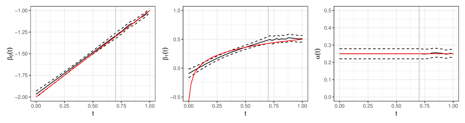
Figure 1: The plot of coefficients for the intercept (left panel), $X_{1}$ (middle panel), and $X_{2}$ (right panel) with 95% confidence bands using the proposed method. The sample size is $n=10^{5}$. The red line represents the true value for each parameter. The coefficient plots are divided at $t=0.75$, corresponding to the estimated coefficient in the training data and one-step ahead prediction in the validation data, respectively.

For our proposed DPSS model, we first divide the data into batches. In the data set, we divide the time into $50$ equally spaced time intervals, $[(s-1)/50,s/50],s=1,2,\cdots,50$. On average, there are $2000$ subjects within each time interval, corresponding to the total sample size of $10^{5}$. We use a normal distribution $N(0,100\cdot I_{5})$ as the initial prior distribution of the coefficients in the model, where $I_{5}$ is the 5-dimensional identity matrix. We use the proposed criterion as in section 3.3 to select the smoothing parameters for $\beta_{0}(t)$ and $\beta_{1}(t)$ using the first 75% data, denoted as $\lambda_{0}$ and $\lambda_{1}$ respectively. Both $\lambda_{0}$ and $\lambda_{1}$ are fixed when making predictions in the remaining data.

We compare the estimated functional curves and corresponding 95% confidence bands for each coefficient of our method. Figure 1 shows the estimated coefficients for the intercept (left panel), $X_{1}$ (middle panel), and $X_{2}$ (right panel) with corresponding 95% confidence bands. The coefficient plots are divided at $t=0.75$ indicated by vertical dotted line, corresponding to the training and validation data, respectively. The figure shows the estimated coefficients in the training set ($t\leq 0.75$) and one-step ahead predicted coefficients in the validation set ($t>0.75$). The estimated coefficient curves using our proposed method are close to the true curves (red lines). In addition, the 95% confidence bands cover the true values in both the training and validation data.

We evaluate the accuracy of the predicted claim of outcome using two different metrics. The first one is Poisson Deviance, which measures how closely the fitted model¡¯s predictions are to the observed outcomes. It is defined as

$$D(y_{i},\hat{y}_{i})=2\sum_{i=1}^{n}\left[y_{i}\log(y_{i}/\hat{y}_{i})-(y_{i}-\hat{y}_{i})\right],$$ (4.1)

where $\hat{y}_{i}$ denotes the predicted mean for on observation $i$ based on the estimated model parameters. A smaller Poisson Deviance means a better model fit. The second one is the difference between predicted and observed data, which is defined as

$$D(\hat{\lambda}_{i},y_{i})=\sum_{i=1}^{n_{test}}I(y_{i}=k)-\sum_{i=1}^{n_{test}}\frac{\hat{\lambda}_{i}^{k}e^{-\hat{\lambda}_{i}}}{k!},\ k=0,1,2,\cdots,$$

where $n_{test}$ is the sample size of test data and $\hat{\lambda}_{i}$ corresponding predicted claim frequency. Table 1 and Table 2 show that our proposed method has much better prediction performance compared with static models (Poisson, NB and ZIP) as the static models are not able to capture the varying effects over time and do not perform well, as one would expect.

Table 1: The Poisson deviance for the testing data in the simulated data set.

Models	Poisson	NB	ZIP	DPSS
Deviance	0.9354	0.9354	0.9178	0.8557

Table 2: The difference between predicted and observed claim frequency for the testing data in the simulated data set.

Count $(k)$	Poisson	NB	ZIP	DPSS
0	3015	3055	3055	24
1	-2139	-2209	-2213	-58
2	-750	-727	-720	9
3	-112	-105	-107	21
4	-14	-13	-13	3
6	-1	-1	-1	-1

5 Empirical analysis

The performance of the DPSS model is tested by using a novel automobile insurance data set in China, which is collected over the years from 2010 to 2015. This data set includes self-reported risk characteristics and claim history with the number of claims, of around 440,000 insurance contracts. The claim data set is collected from three types of automobile insurance, including collision insurance, third-party liability insurance, and compulsory traffic insurance. Table 3 presents the distribution of the number of claims over time. We observe that most policyholders do not have a claim (82.10%), some have one or two claims (16.4%) and the remaining policyholders have more than three claims. The probability of having no claim is increasing over years, especially from 2014 to 2015. We argue that the Chinese regulator has launched a comprehensive 2nd reform of the automobile insurance segment from 2007 to 2015, followed by a 3rd reform from 2015 to 2020, covering pricing, fee structures, and product coverage among others, which had a big impact on the distribution of the number of claims. Especially around 2014-2015, China launched the auto insurance reform by expanding insurance coverage, adopting a uniform ratemaking mechanism to address the problem of “high premiums and low compensation” in the Chinese automobile insurance market. This changing regulatory policy motivates us to take the time trend into the statistical models when we aim to predict the claim frequency beyond the sample period.

The information on risk characteristics of the individual policies in this data set contains: expo, gender, age, carage, carvalue, ptype, carusage, svolume, carseats and coverage. The summary statistics of these variables are shown in Table 4. Figure 2 shows how the covariates are distributed in the automobile insurance data set over years. Most policyholders (70.90%) are exposed to the risk of filing a claim during a whole policy year, while the others between zero and one, which indicates that the underwriting date of those policies might be after the start of the year, or surrender of the contract occurs before the end of the year. Almost all policyholders (89.12%) are aged between 25 and 60, which means that there are few young and old policyholders in the insurance portfolio, and more than half of the policyholders (75.96%) are female. Most policies (78.59%) are renewed or transferred from other insurance companies. More than half of vehicles (76.20%) have a displacement of less than 1.6 L, half of the vehicles (50.73%) are domestic, 79.05% of vehicles have a seating capacity of fewer than 6 seats and 66.57% of vehicles are sedans. More than half of policies (60.60%) do not cover all three types of insurance: collision insurance, third-party liability insurance, and compulsory traffic insurance.

Table 3: Distribution of numbers of claims over years in automobile insurance data set.

Count	Percentage by Year
	2010	2011	2012	2013	2014	2015	Overall
0	77.20%	77.90%	78.70%	78.70%	82.10%	94.70%	82.10%
1	15.00%	14.80%	14.20%	14.50%	13.60%	4.70%	12.60%
2	5.10%	5.00%	5.00%	5.00%	3.50%	0.50%	3.80%
3	1.70%	1.60%	1.50%	1.40%	0.70%	0.10%	1.10%
4+	1.00%	0.70%	0.50%	0.40%	0.20%	0.00%	0.40%
obs.	39,103	51,604	75,298	91,418	106,076	79,012	442,511

Table 4: Description of the risk characteristics in automobile insurance data set.

Variables	Type	Description
expo	continuous	risk exposures measured by the effective policy duration: 0-1
age	continuous	age of the policyholders: 18-99
carage	continuous	age of vehicle: 0-13
carvalue	continuous	log transformation of purchase price of the vehicle: 9.8 (minimum) -16 (maximum)
ptype	categorical	policy type (two levels): newly underwritten policy with new vehicle (new), renewal policy or transferred policy from other insurance company (renewal or transferred)
carusage	categorical	categories of vehicle (two levels): sedans and non-sedans
carorigin	categorical	two levels: domestic or non-domestic vehicles
svolume	categorical	swept volume of vehicle (two levels): $>1.6L$ or $\leq 1.6L$
carseats	categorical	number of seats in vehicle (two levels): $\geq 6$ seats or $<6$ seats
coverage	categorical	insurance coverage of vehicle (two levels): covering collision insurance, third-party liability insurance and compulsory traffic insurance (coverage_all), or not covering three types of insurance (coverage_else)
gender	categorical	male or female

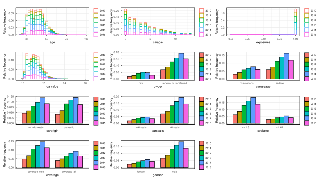
Figure 2: Relative frequency of the covariates expo, gender, age, carage, carvalue, ptype, carusage, carorigin, svolume, carseats and coverage over years.

We first fit a DPSS to model the number of claims that allows the intercept and coefficients for all the above-mentioned predictors to change over time. Specifically, the data set is split into six batches by year. The first five batches (data from years 2010-2014, denoted by $\mathcal{L}(Y_{i}(k),\bm{x}_{i}(k))_{0\leq i\leq n},k=2010,\dots,2014$) are used as the training data for model fitting and smoothing parameter selection, and the sixth batch data (data from 2015, denoted by $\mathcal{L}(Y_{i}(k),\bm{x}_{i}(k))_{0\leq i\leq n},k=2015$) is used as the testing data for an out-of-sample analysis. The preliminary analysis shows that only the coefficients of age, carage and carvalue are constant over time while the others keep changing over time. Now, we consider the following DPSS:

$$\log\lambda_{i}(t_{i})= \beta_{0}(t_{i})+\beta_{1}(t_{i})\log\mathrm{expo}+\beta_{2}(t_{i})\mathrm{caruseage}_{i}+\beta_{3}(t_{i})\mathrm{carseats}_{i}+\beta_{4}(t_{i})\mathrm{ptype}_{i}$$

$$\quad+\beta_{5}(t_{i})\mathrm{coverage}_{i}+\beta_{6}(t_{i})\mathrm{gender}_{i}+\beta_{7}(t_{i})\mathrm{svolume}_{i}+\beta_{8}(t_{i})\mathrm{carorigin}_{i}$$

$$\quad+\alpha_{1}\mathrm{age}_{i}+\alpha_{2}\mathrm{carage}_{i}+\alpha_{3}\mathrm{carvalue}_{i}.$$

Note that binary coding is employed for the categorical variables (gender, ptype, carusage, carorigin, svolume, carseats and coverage). To illustrate the superiority of the proposed models, we also consider five competing regression models: Poisson regression model (Poisson), negative-binomial regression model (NB), and zero-inflated Poisson regression model (ZIP), as well as the Dynamic negative-binomial state space model (DNBSS) and Dynamic zero-inflated Poisson state space model (DZIPSS). The year $t_{i}$ as a continuous covariate is introduced into the mean parameter to capture the time trend over years in static models. The mean of the Poisson component and the probability of extra zeros are both assumed to be modelled as the function of the covariates in the ZIP model.

Figure 3(a)-(i) plot the estimated varying coefficients for the intercept and eight covariates of the DPSS model with 95% confidence bands as the function of years 2010-2014 in the training data and year 2015 in the testing data. From Figure 3(c)-(e), we observed that the claim frequency of sedans is higher than non-sedans; vehicles with fewer than six seats are claimed more frequently than vehicles with more than six seats; domestic vehicles have more claims than non-domestic vehicles. The difference in claim frequency between sedans and non-sedans has a slightly decreasing trend from 2010 to 2011, then increases from 2011 to 2013 and decreases after 2013. A similar time trend can be observed in Figure 3(d) and (e). From the time plot of the coverage variable in Figure 3(f), we can see that the difference in claim frequency between policies with high insurance coverage and policies with low coverage shows an increasing trend before 2012 followed by a decreasing trend. The positive estimated coefficient indicates that the policies with high insurance coverage have a relatively high claim frequency. There are two possible reasons for this: (1) drivers with bad driving habits are the ones who buy insurance with high insurance coverage; (2) the drivers with high insurance coverage drive more casually, resulting in more insurance claims. Figure 3(g) shows that while the female has more claims than the male, the difference in claim frequency is decreasing over time and even tends to be zero after the year 2014. In Figure 3(i), the decreasing time trend of ptype can be observed, which indicates that the renewed or transferred policies have more claim frequency than new policies. Another interesting finding is that the sign of the estimated coefficient of svolume in Figure 3(h) changes from negative to positive as the year increases. Overall, we can conduct that the time trend of most of the rating factors changes around 2011-2012, and the impact on claim frequency is decreasing over time. The time plots indicate that rating factors play less important roles in classification rate-making as the year increases, which is in line with the timeline of the second round of insurance rate reform that was conducted in 2007-2015 with the aim of reducing the insurance premium rate and increasing the insurance coverage. The most important regulations for this round of reform were the “Motor Vehicle Commercial Insurance Model Clauses” issued by The Insurance Association of China in 2012 , and the “Opinions on deepening the reform of commercial auto insurance terms and rates management system” issued by China Banking and Insurance Regulatory Commission in 2015 . The uniform vehicle insurance terms and conditions were suggested by regulatory authorities during this period for automobile insurance rate-making to avoid vicious competition by insurance companies to attract customers by reducing premiums. These changing regulations weakened the right of insurance companies to set premiums based on risk classification, which reflected a decreasing trend of estimated regression coefficients for most of the rating factors.

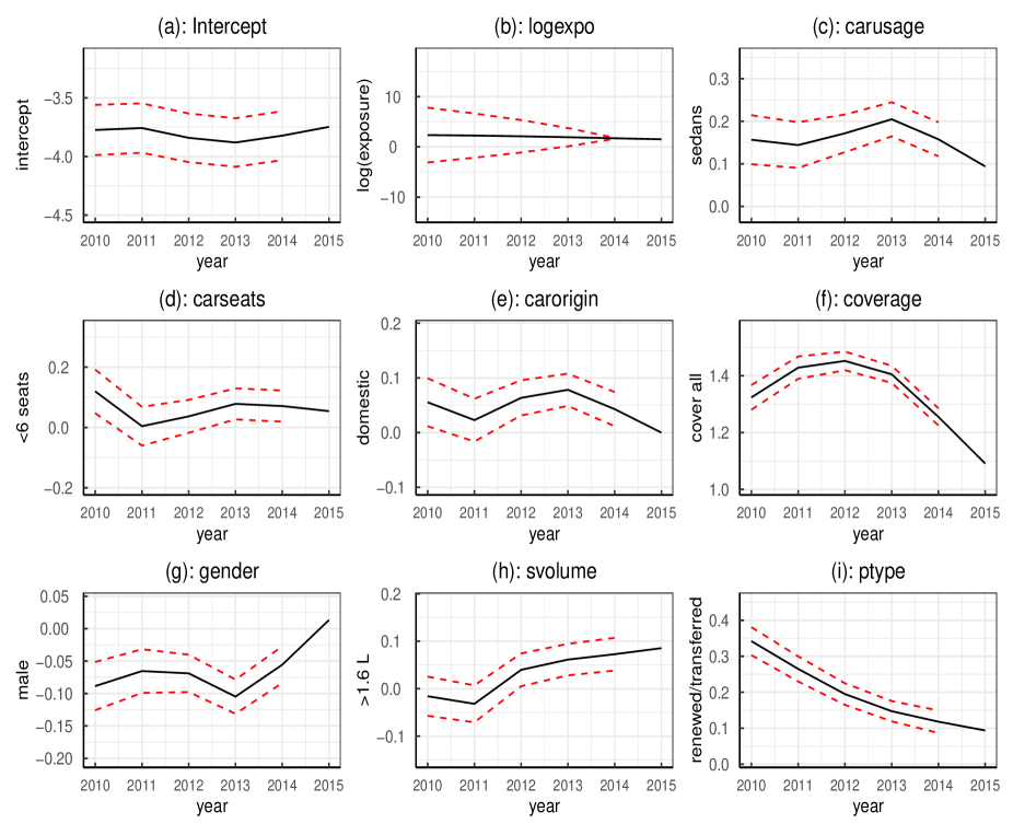
Figure 3: The plot of coefficients for the intercept (left) and eight covariates with 95% confidence bands using the proposed method. The coefficient plots are divided at $t=0.75$, corresponding to the estimated coefficient in the training data and one-step ahead prediction in the testing data, respectively. Female in gender variable, new policy in ptype, non-sedans in caruseage, non-domestic in carorigin, $\leq 1.6$L in svolume, $\geq 6$ seats in carseats and coverage_else in coverage are used for the reference levels.

To compare the performance of Poisson, NB, ZIP, DPSS, DNBSS, and DZIPSS models, we predict the claim frequency by applying each model on the testing data. Table 5 reports the difference between predicted and observed claims for the testing data. One can see that our proposed dynamic prediction models have much better performance in predicting the claim frequency having no claims. Figure 4 shows the predicted total number of claims for the whole insurance portfolio in the testing data. The static prediction models (Poisson, NB, ZIP) overestimate the total number of claims, while DPSS and DNBSS underestimate the true value. DZIPSS has the best prediction performance as it has the lowest deviation. The predicting outcomes of dynamic models are much closer to observed total number of claims than static models. We also evaluate the accuracy of the predicted claim of outcome using the Poisson Deviance defined in (4.1), the lifts discussed in (Lee, 2021) and Gini index proposed by Frees et al. (2011). The lifts and the Gini index are auxiliary metrics that evaluate the models without an assumption on the underlying distribution. The lifts are the ratio of the the average response of the top decile prediction over the average response of the bottom decile (for two-way) and the population (for one-way). The lift can be interpreted as a measure of the ability of a model to differentiate observations. A higher lift illustrates that the model is more capable of separating the extreme values from the average. A similar auxiliary metric is the Gini index, which is a measure of assessing the discriminatory power of the models, especially for the claim data with the high proportions of zeros and the highly right-skewed features. A score with a greater Gini index produces a greater separation among the observations. In other words, a higher Gini index indicates a greater ability to distinguish good risks from bad risks. From Table 6, one can see that dynamic models (DPSS, DNBSS, and ZIPSS) have the smaller Deviance than the static models (Poisson, NB, and ZIP), which indicates that the model fitting performance can be improved by introducing the time trend of the rating factors. The one-way lifts for DPSS and Poisson models are 3.522 and 3.550 respectively, which indicates that the top 10% risk classified by the DPSS model contributes around 35.22% of the total claims according to the one-way lift, while the top 10% risk classified by static Poisson contributes around 35.50%. This means insurers can remove the top 10% of risks through underwriting, and the remaining 90% of the policy represents only 64.78% of the original loss according to the results of DPSS. The insurers will charge 28.02% (1-64.78/90) lower on average based on the DPSS model while 28.33% (1-64.50/90) based on the static Poisson model. Smaller one-way and two-way lifts in dynamic models are observed, which indicates that dynamic models do not show a better ability to distinguish good risks from bad risks. The results are in line with the objectives of the second round of insurance rate reform in China that was conducted in 2007-2015 with the aim of weakening the risk differentiation ability of the rating factors. Table 6 shows that there is no significant difference in the risk differentiation ability of these six models in terms of the Gini index.

From Figure 5, we can also assess the performance of the candidates by utilizing the lift plot (Lee, 2021). To derive the measure, we sort the prediction and group the observations into 10 deciles. Figure 5 shows the average responses over average predictions for the deciles. If the points are aligned with 45 degree line, the model has a high predictive performance. From Figure 5, we see that dynamic models perform extremely well in predicting high-frequency risk classes as the prediction and response are almost the same. Figure 6 shows the double lift plot, which provides a direct predictive performance comparison between the DPSS model over the Poisson model. The double lift plot is discussed in details in the work of Lee (2020). We can see a significantly positive relationship between the blue line (loss ration) and the red line (indicated rate change), with a correlation of 0.963, indicating the DPSS model is able to explains a high portion of residuals that the Poisson model fails to capture.

Table 5: The difference between predicted and observed claims for the testing data in the real data set.

Count $(k)$	Static models			Dynamic models
	Poisson	NB	ZIP	DPSS	DNBSS	DZIPSS
0	-1353	-1058	-1032	526	685	-222
1	1342	828	838	-309	-555	268
2	27	172	172	-181	-113	-25
3	-12	44	21	-31	-15	-16
4	-3	11	1	-5	-2	-4
5	-1	2	0	-1	-1	-1
6	0	1	0	0	0	0

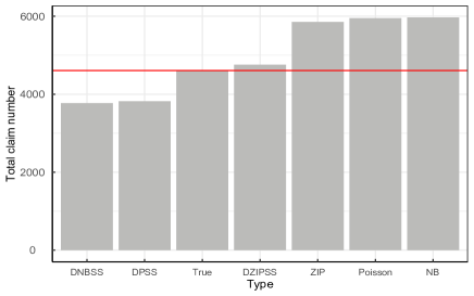
Figure 4: The predicted value of the total numbers of claim for the testing data. The true observation of the total numbers of claim is 4,068, which is marked as the red line.

Table 6: The Poisson deviance, lifts and Gini index for the testing data in the real data set.

Models	Static models			Dynamic models
	Poisson	NB	ZIP	DPSS	DNBSS	DZIPSS
Poisson Deviance	0.300	0.300	0.299	0.299	0.300	0.296
Two-way Lift	1.735	1.711	1.707	1.608	1.581	1.701
One-way Lift	3.550	3.530	3.537	3.522	3.507	3.576
Gini index	0.934	0.934	0.934	0.934	0.934	0.934

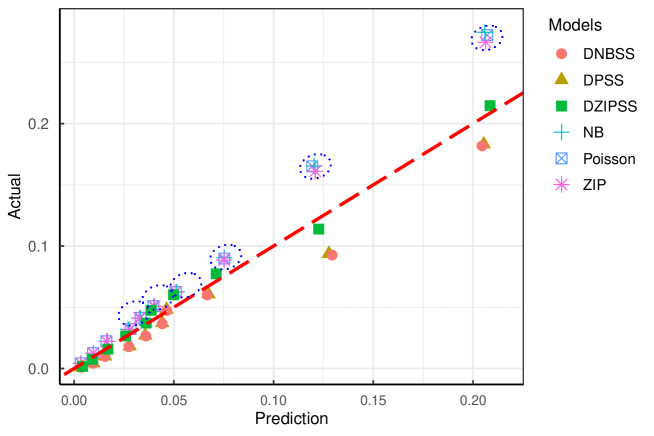
Figure 5: Lift plot for competing models. Static models are circled by dark blue dotted lines.

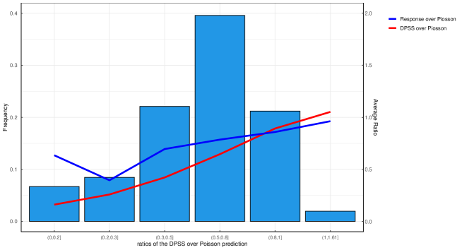
Figure 6: Double lift plot for DPSS model over Poisson model. Observations are sorted in the ratios of the DPSS over the Poisson prediction and are grouped by the intervals that they belong (ratio of $0.6\in(0.5,0.8]$). For each bucket, the ratio of actual claim counts over total Poisson prediction is marked as the blue line, and the ratio of total DPSS prediction over total Poisson prediction is marked as the red line.

6 Conclusion

We have proposed and studied the Dynamic Poisson state space model and its extensions to not only handle very unbalance claim data with excessive proportion of zeros, but update the prediction of claim frequency over time by the state space modelling framework. Unlike Bayesian estimation methods used in state space models which are frequently discussed in the existing actuarial science literature (Ahn et al., 2022), the parameters in our proposed model are modelled by the smoothing splines over time and are estimated via maximum likelihood method. The prediction for claim frequency is based on Kalman filter like algorithm and can be updated dynamic when new claim information becomes available. The proposed method overcomes the limitations of traditional varying-coefficients models which mainly focus on estimation and statistical inference rather than the future prediction. It is also designed for online monitoring as the proposed algorithm has better computational efficiency than Bayesian estimation method. In a real-world insurance claim data set, we model the claim counts data over six years as the function of several covariates in the Poisson, negative-binomial and zero-inflated Poisson assumptions and update the models every one year. The empirical results show that the dynamic pattern of the estimated coefficients in DPSS for most of rating factors can be explained by the process of auto insurance rate reform in China from year 2010 to 2015. Several practical metrics reveal the superiority of the proposed method in predicting claim frequency.

It is worth mentioning that the DPSS we proposed in this work were univariate count models, and it would be extended to multivariate count models when the frequency of automobile claims contains more than one types, for example the number of claims of third-party bodily injury ($Y_{1}$), the number of claims of own damage ($Y_{2}$), and the number of claims of third party property damage ($Y_{3}$). Another extension of this work could be devoted to the spatial analysis in the dynamic state space setting that allows us to investigate more complex effects of the covariates on the insurance claim data. Besides, the dynamic modelling approach based state space equations could be further discussed for longitudinal claim data in the experience ratemaking context.

Supplementary materials

Code: The R source code for Dynamic Poisson state space model and simulation study. A readme file is included in the archive (dpss.zip).

Appendices

A Dynamic zero-inflated Poisson state space model (DZPSS)

Suppose the response variable $y_{i}$ is zero-inflated Poisson distribution with the mean $e_{i}\lambda_{i}$ and the zero-inflated probability $\phi_{i}$, that is

$${{Y}_{i}}\sim\left\{\begin{matrix}&0,&\text{with}\text{ probability}\quad{{\phi}_{i}},\\ &\text{Poisson}\left({{\lambda}_{i}}\right),&\text{with}\text{ probability }1-{{\phi}_{i}},\\ \end{matrix}\right.$$ (.1)

In (.1), $0\leq\phi_{i}<1$, so extra zeros in the data can be explicitly modelled. The additional point mass at 0 allows ZIP model to produce more responses with value 0 than those predicted by the Poisson distribution, and thus accommodates the zero-inflated phenomenon.

The effects of covariates with time-varying and time-invariant coefficients can be modelled as

$$\log\left({{\lambda}_{i}}\right) =\bm{B}_{i,q_{1}}^{T}\bm{\beta}\left({{t}_{i}}\right)+\bm{B}_{i,q_{2}}^{T}\bm{\varphi}={{\bm{B}}^{T}_{i}}\bm{\gamma}\left({{t}_{i}}\right),$$

$$\text{logit}\left({{\phi}_{{i}}}\right) =\log\left(\frac{\phi_{i}}{1-\phi_{i}}\right)=\bm{G}_{i,q_{1}}^{T}\bm{\rho}\left({{t}_{i}}\right)+\bm{G}_{i,q_{2}}^{T}{{\bm{\alpha}}}={{\bm{G}}^{T}_{i}}\bm{\gamma}\left({{t}_{i}}\right),$$ (.2)

where ${{\bm{B}}_{i,q_{1}}}={{\left(1,{{B}_{i,1}},\cdots,{{B}_{i,q_{1}}}\right)}^{T}}$ and ${{\bm{G}}_{i,q_{1}}}={{\left(1,{{G}_{i,1}},\cdots,{{G}_{i,q_{1}}}\right)}^{T}}$ are the covariates with time varying coefficients $\bm{\beta}\left(t\right)={{\left({{\beta}_{0}}\left(t\right),\cdots,{{\beta}_{q_{1}}}\left(t\right)\right)}^{T}}$ and $\bm{\rho}\left(t\right)={{\left({{\rho}_{0}}\left(t\right),,{{\rho}_{q_{1}}}\left(t\right)\right)}^{T}}$. ${{\bm{B}}_{i,q_{2}}}={{\left(1,{{B}_{i,1}},\cdots,{{B}_{i,q_{2}}}\right)}^{T}}$ and ${{\bm{G}}_{i,q_{2}}}={{\left(1,{{G}_{i,1}},\cdots,{{G}_{i,q_{2}}}\right)}^{T}}$ are the covariates with time-invariant coefficients $\bm{\varphi}={{\left({{\varphi}_{1}},\cdots,{{\varphi}_{q_{2}}}\right)}^{T}}$ and $\bm{\alpha}={{\left({{\alpha}_{1}},\cdots,{{\alpha}_{q_{2}}}\right)}^{T}}$. ${{\bm{B}}_{i}}={{\left({\bm{B}}_{i,q_{1}}^{T},{\bm{B}}_{i,q_{2}}^{T},0,\cdots,0\right)}^{T}}$ and ${{\bm{G}}_{i}}={{\left(0,\cdots,0,G_{i,q_{1}}^{T},G_{i,q_{2}}^{T}\right)}^{T}}$ are the $2(q_{1}+q_{2}+1)$-dimensional vector of covariates with vector of coefficients $\bm{\gamma}\left(t\right)={{\left(\bm{\beta}{{\left(t\right)}^{T}},{\bm{\varphi}^{T}},\bm{\rho}{{\left(t\right)}^{T}},{\bm{\alpha}^{T}}\right)}^{T}}$.

The parameters can be estimated through maximizing the following penalized log-likelihood function:

$${{L}_{c}}\left(\bm{\gamma};\bm{y}\right) =\sum\limits_{{{y}_{i}}=0}{\log\left\{{{e}^{{{\bm{G}}^{T}_{i}}\bm{\gamma}\left({{t}_{i}}\right)}}+\exp\left[-{{e}^{{{\bm{B}}^{T}_{i}}\bm{\gamma}\left({{t}_{i}}\right)}}\right]\right\}}+\sum\limits_{{{y}_{i}}>0}{\left[{{y}_{i}}{{\bm{B}}^{T}_{i}}\bm{\gamma}\left({{t}_{i}}\right)-{{e}^{{{\bm{B}}^{T}_{i}}\bm{\gamma}\left({{t}_{i}}\right)}}-\log\left({{y}_{i}}!\right)\right]}$$

$$\quad-\sum\limits_{i=1}^{n}{\log\left[1+{{e}^{{{\bm{G}}^{T}_{i}}\bm{\gamma}\left({{t}_{i}}\right)}}\right]}-\frac{1}{2}\sum\nolimits_{j=0}^{q_{1}}{{{\tau}_{1j}}\int{{{\left\{{{\bm{\beta}}_{j}}^{{}^{\prime\prime}}\left(t\right)\right\}}^{2}}dt-\frac{1}{2}\sum\nolimits_{j=0}^{q_{1}}{\tau}_{2j}\int{\left\{{{\bm{\rho}}_{j}}^{{}^{\prime\prime}}\left(t\right)\right\}}^{2}dt,}}$$

Similar to the DPSS proposed in (2.1), the DZIPSS (.2) can be also represented in a state space representation as

$$\log\left({{\lambda}_{i}}\right) ={{\bm{U}}^{T}_{{i}}}\bm{\zeta}\left({{t}_{i}}\right),$$

$$\text{logit}\left({{\phi}_{i}}\right) ={{\bm{V}}^{T}_{{i}}}\bm{\zeta}\left({{t}_{i}}\right),$$

$$\bm{\zeta}\left({{t}_{i}}\right) ={{\bm{T}}_{{i}}}\bm{\zeta}\left({{t}_{i-1}}\right)+\bm{\eta}\left({{t}_{i}},{{t}_{i-1}}\right),\quad\bm{\eta}\left({{t}_{i}},{{t}_{i-1}}\right)\sim N\left(\bm{0,}{{\bm{Q}}_{i}}\right),$$ (.3)

where

$${\bm{U}_{i}}={{\left(1,0,{{B}_{i1}},0,{{B}_{i2}},\cdots,{{B}_{i{{q_{1}}}}},0,{{B}_{i{{q_{1}+1}}}},{{B}_{i{{q_{1}+2}}}},\cdots,{{B}_{i{{q_{1}+q_{2}}}}},0,0,\cdots,0\right)}^{T}},$$

$${\bm{V}_{i}}={{\left(0,0,\cdots,0,1,0,{{G}_{i1}},0,{{G}_{i2}},\cdots,{{G}_{i{{q_{1}}}}},0,{{G}_{i{{q_{1}+1}}}},{{G}_{i{{q_{1}+2}}}},\cdots,{{G}_{i{{q_{1}+q_{2}}}}}\right)}^{T}},$$

$$\bm{\zeta}\left(t\right)={{\left({{\beta}_{0}}\left({{t}_{i}}\right),{{\beta}_{0}}^{\prime}\left({{t}_{i}}\right),\cdots,{{\beta}_{q_{1}}}\left({{t}_{i}}\right),{{\beta}_{q_{1}}}^{\prime}\left({{t}_{i}}\right),{\bm{\varphi}^{T}},{{\rho}_{0}}\left({{t}_{i}}\right),{{\rho}_{0}}^{\prime}\left({{t}_{i}}\right),\cdots,{{\rho}_{q_{2}}}\left({{t}_{i}}\right),{{\rho}_{q_{2}}}^{\prime}\left({{t}_{i}}\right),{\bm{\alpha}^{T}}\right)}^{T}},$$

$${{\bm{T}}_{i}}=\text{diag}(\overbrace{{{T}_{i}},\cdots,{{T}_{i}}}^{{{q}_{1}}+1},\overbrace{1,\cdots,1}^{{{q}_{2}}},\overbrace{{{T}_{i}},\cdots,{{T}_{i}}}^{{{q}_{1}}+1},\overbrace{1,\cdots,1}^{{{q}_{2}}}),$$

$${{\bm{Q}}_{\text{i}}}=\text{diag}(\overbrace{\tau_{10}^{-1}{{Q}_{i}},\cdots,\tau_{1{{q}_{1}}}^{-1}{{Q}_{i}}}^{{{q}_{1}}+1},\overbrace{0,\cdots,0}^{{{q}_{2}}},\overbrace{\tau_{20}^{-1}{{Q}_{i}},\cdots,\tau_{2{{q}_{1}}}^{-1}{{Q}_{i}}}^{{{q}_{1}}+1},\overbrace{0,\cdots,0}^{{{q}_{2}}}).$$

The estimation and prediction algorithm is similar to model (2.6).

B Dynamic negative-binomial state space model (DNBPSS)

The negative-binomial model can arise from a two-stage model for the distribution of a discrete variable $Y$. We suppose there is an unobserved random variable $\Theta$ have a Gamma distribution $\Theta\sim\text{Gamma}(\alpha,\alpha)$ with mean $1$ and variance $1/\alpha$. Then the model postulates that conditionally on $\Theta$, $Y$ is Poisson with mean $\mu\Theta$. Then the marginal distribution of $Y$ is the negative-binomial distribution with mean $\mu$ and variance $\mu+1/\alpha\mu^{2}$. The effects of covariates with time-varying and time-invariant coefficients in the Dynamic negative-binomial state space model can be introduced in the mean $\mu$ of the negative-binomial distribution, that is

$$\log\left(\mu_{i}\right) =\bm{z}_{i}^{T}\bm{\gamma}\left({{t}_{i}}\right),\ \ \ \ i=1,\cdots,n$$

$$\bm{\gamma}\left({{t}_{i}}\right) ={\bm{T}_{i}}\bm{\gamma}\left({{t}_{i}}\right)+\bm{\eta}\left({{t}_{i}},{{t}_{i-1}}\right),\ \ \bm{\eta}\left({{t}_{i}},{{t}_{i-1}}\right)\sim N\left(\bm{0},{\bm{Q}_{i}}\right),$$ (.4)

where

$${\bm{z}_{i}} ={{\left(1,0,{{x}_{i1}},0,{{x}_{i2}},\cdots,{{x}_{i{{q}_{1}}}},0,{{x}_{i,{{q}_{1}}+1}},\cdots,{{x}_{iq}}\right)}^{T}},$$

$$\bm{\gamma}\left(t\right) ={{\left({{\beta}_{0}}\left(t\right),{{{{\beta}^{\prime}}}_{0}}\left(t\right),{{\beta}_{1}}\left(t\right),{{{{\beta}^{\prime}}}_{1}}\left(t\right),\cdots,{{\beta}_{{{q}_{1}}}}\left(t\right),{{{{\beta}^{\prime}}}_{{{q}_{1}}}}\left(t\right),{{\alpha}_{1}},\cdots,{{\alpha}_{{{q}_{2}}}}\right)}^{T}},$$

$$\bm{\eta}\left({{t}_{i}},{{t}_{i-1}}\right) ={{\left(U_{0}^{T}\left({{t}_{i}},{{t}_{i-1}}\right),\cdots,U_{{{q}_{1}}}^{T}\left({{t}_{i}},{{t}_{i-1}}\right)\right)}^{T}},$$

$${\bm{T}} =\text{diag}\left(\overbrace{{{T}},\cdots,{{T}}}^{{{q}_{1}}+1},\overbrace{1,\cdots,1}^{{{q}_{2}}}\right),{\bm{Q}}=\text{diag}\left(\overbrace{\lambda_{0}^{-1}{{Q}},\cdots,\lambda_{{{q}_{1}}}^{-1}{{Q}}}^{{{q}_{1}}+1},\overbrace{0,\cdots,0}^{{{q}_{2}}}\right).$$

References

- Ahn et al. (2022) Jae Youn Ahn, Himchan Jeong, and Yang Lu. A simple bayesian state-space approach to the collective risk models. Scandinavian Actuarial Journal, pages 1–21, 2022.
- Bhattacharjee et al. (2018) Atanu Bhattacharjee, Gajendra K Vishwakarma, and Abin Thomas. Bayesian state-space modeling in gene expression data analysis: An application with biomarker prediction. Mathematical biosciences, 305:96–101, 2018.
- Chang and Shi (2020) Le Chang and Yanlin Shi. Dynamic modelling and coherent forecasting of mortality rates: a time-varying coefficient spatial-temporal autoregressive approach. Scandinavian Actuarial Journal, 2020(9):843–863, 2020.
- Denuit and Lu (2021) Michel Denuit and Yang Lu. Wishart-gamma random effects models with applications to nonlife insurance. Journal of Risk and Insurance, 88(2):443–481, 2021.
- Dong and Chan (2013) A.X.D. Dong and J.S.K. Chan. Bayesian analysis of loss reserving using dynamic models with generalized beta distribution. Insurance: Mathematics and Economics, 53(2):355–365, 2013.
- Fan and Zhang (2008) Jianqing Fan and Wenyang Zhang. Statistical methods with varying coefficient models. Statistics and its Interface, 1(1):179–195, 2008.
- Frees et al. (2011) Edward W Frees, Glenn Meyers, and A David Cummings. Summarizing insurance scores using a gini index. Journal of the American Statistical Association, 106(495):1085–1098, 2011.
- Fung et al. (2017) Man Chung Fung, Gareth W. Peters, and Pavel V. Shevchenko. A unified approach to mortality modelling using state-space framework: characterisation, identification, estimation and forecasting. Annals of Actuarial Science, 11(2):343–389, 2017.
- Gu (1992) Chong Gu. Penalized likelihood regression: a bayesian analysis. Statistica Sinica, pages 255–264, 1992.
- Hastie and Tibshirani (1993) Trevor Hastie and Robert Tibshirani. Varying-coefficient models. Journal of the Royal Statistical Society: Series B (Methodological), 55(4):757–779, 1993.
- Henckaerts and Antonio (2022) Roel Henckaerts and Katrien Antonio. The added value of dynamically updating motor insurance prices with telematics collected driving behavior data. Insurance: Mathematics and Economics, 105:79–95, 2022.
- Hilbe (2011) Joseph M Hilbe. Negative binomial regression. Cambridge University Press, 2011.
- Jiang et al. (2021) Jiakun Jiang, Wei Yang, Erin M Schnellinger, Stephen E Kimmel, and Wensheng Guo. Dynamic logistic state space prediction model for clinical decision making. Biometrics, 2021.
- Jørgensen and Smyth (1994) Bent Jørgensen and Gorden Smyth. Fitting tweedie’s compound poisson model to insurance claims data. Scandinavian Actuarial Journal, 1994:69–93, 01 1994.
- Klein et al. (2015) Nadja Klein, Thomas Kneib, and Stefan Lang. Bayesian generalized additive models for location, scale, and shape for zero-inflated and overdispersed count data. Journal of the American Statistical Association, 110(509):405–419, 2015.
- Lai and Sun (2012) Tze Leung Lai and Kevin Haoyu Sun. Evolutionary credibility theory: A generalized linear mixed modeling approach. North American Actuarial Journal, 16(2):273–284, 2012.
- Lambert (1992) Diane Lambert. Zero-inflated poisson regression, with an application to defects in manufacturing. Technometrics, 34(1):1–14, 1992.
- Lee (2020) Simon CK Lee. Delta boosting implementation of negative binomial regression in actuarial pricing. Risks, 8(1), 2020.
- Lee (2021) Simon CK Lee. Addressing imbalanced insurance data through zero-inflated poisson regression with boosting. ASTIN Bulletin: The Journal of the IAA, 51(1):27–55, 2021.
- Lee et al. (2020) Woojoo Lee, Jeonghwan Kim, and Jae Youn Ahn. The poisson random effect model for experience ratemaking: limitations and alternative solutions. Insurance: Mathematics and Economics, 91:26–36, 2020.
- Lewis and Raftery (1997a) Steven M. Lewis and Adrian E. Raftery. Estimating bayes factors via posterior simulation with the laplace—metropolis estimator. Journal of the American Statistical Association, 92(438):648–655, 1997a.
- Lewis and Raftery (1997b) Steven M Lewis and Adrian E Raftery. Estimating bayes factors via posterior simulation with the laplace—metropolis estimator. Journal of the American Statistical Association, 92(438):648–655, 1997b.
- Li et al. (2021) Hong Li, Yang Lu, and Wenjun Zhu. Dynamic bayesian ratemaking: A markov chain approximation approach. North American Actuarial Journal, 25(2):186–205, 2021.
- Lu (2018) Yang Lu. Dynamic frailty count process in insurance: A unified framework for estimation, pricing, and forecasting. Journal of Risk and Insurance, 85(4):1083–1102, 2018.
- O’Neill (2002) Philip D O’Neill. A tutorial introduction to bayesian inference for stochastic epidemic models using markov chain monte carlo methods. Mathematical Biosciences, 180(1-2):103–114, 2002.
- Park et al. (2015) Byeong U Park, Enno Mammen, Young K Lee, and Eun Ryung Lee. Varying coefficient regression models: a review and new developments. International Statistical Review, 83(1):36–64, 2015.
- Pinquet (2020) Jean Pinquet. Poisson models with dynamic random effects and nonnegative credibilities per period. ASTIN Bulletin: The Journal of the IAA, 50(2):585–618, 2020.
- Taylor (2018) Greg Taylor. Evolutionary hierarchical credibility. ASTIN Bulletin: The Journal of the IAA, 48(1):339–374, 2018.
- Wahba (1978) Grace Wahba. Improper priors, spline smoothing and the problem of guarding against model errors in regression. Journal of the Royal Statistical Society: Series B (Methodological), 40(3):364–372, 1978.
- Wahba (1983) Grace Wahba. Bayesian “confidence intervals” for the cross-validated smoothing spline. Journal of the Royal Statistical Society: Series B (Methodological), 45(1):133–150, 1983.
- Wecker and Ansley (1983) William E Wecker and Craig F Ansley. The signal extraction approach to nonlinear regression and spline smoothing. Journal of the American Statistical Association, 78(381):81–89, 1983.
- Yip and Yau (2005) Karen CH Yip and Kelvin KW Yau. On modeling claim frequency data in general insurance with extra zeros. Insurance: Mathematics and Economics, 36(2):153–163, 2005.
- Zhu et al. (2011) Ying Zhu, Barry K Goodwin, and Sujit K Ghosh. Modeling yield risk under technological change: Dynamic yield distributions and the us crop insurance program. Journal of Agricultural and Resource Economics, pages 192–210, 2011.