A note on the rate of convergence of integration schemes for closed surfaces

Abstract

In this paper, we issue an error analysis for integration over discrete surfaces using the surface parametrization presented in [PS22] as well as prove why even-degree polynomials utilized for approximating both the smooth surface and the integrand exhibit a higher convergence rate than odd-degree polynomials. Additionally, we provide some numerical examples that illustrate our findings and propose a potential approach that overcomes the problems associated with the original one.

Keywords numerical integration; surface integrals; convergence rates; closest point projection; Chebyshev-Lobatto nodes.

1 Introduction

Many applications, including mathematical physics and mathematical biology [YQ09], require accurate approximation of integrals on curved surfaces. The concept of surface integration is a fundamental procedure in a wide range of numerical methods, including the boundary integral method, the finite element method, the surface finite element method, and the finite volume method. As a result of piecewise linear approximations of the surface and integrand, integration over discrete surfaces (such as surface triangulation) is typically only of first- or second-order accuracy [Geo98]. To improve the order of accuracy, using the approach presented in [PS22] a polynomial approximation of the geometry of a smooth closed embedded hypersurface $\mathcal{M}$ is considered, where a local interpolation polynomial of the closest point projection map $\pi$ for each element $T\in\mathcal{T}^{1}_{h}$ will be constructed, with $\mathcal{T}^{1}_{h}$ denoting a conforming triangulation of $\mathcal{M}$.

The contribution of this paper is twofold. First, we deliver a parametrization of smooth, closed surfaces, enabling to numerically approximate surface integrals based on discrete triangulations. That is approximately providing a decomposition $\mathcal{M}=\bigcup_{i=1}^{n}V_{i}$ into non-overlapping regions $V_{i}$, given as images of regular maps, see Fig. (1)

$$\psi_{i}:\sigma\longrightarrow V_{i}\subseteq\mathcal{M}\,,$$ (1.1)

where $\sigma$ is a reference simplex defined as $\sigma:=\{\left(s,t\right),0\leq s\leq 1,0\leq t\leq 1-s\}\,$ in $\mathbb{R}^{2}$.

Figure 1: Representation of a smooth surface parametrization, where every region $V_{i}$ forms a curved triangle.

Consequently, the surface integration problem becomes:

$$\int_{\mathcal{M}}fdS=\sum_{i=1}^{n}\int_{V_{i}}fdS=\sum_{i=1}^{n}\int_{0}^{1}\int_{0}^{1-s}f\big{(}\psi_{i}(s,t)\big{)}g_{i}(s,t)dsdt\,,$$ (1.2)

where $g_{i}(s,t)=\sqrt{\det(J^{T}J)}$ with $J=[\partial_{s}\psi_{i}(s,t),\partial_{t}\psi_{i}(s,t)]$ and $\partial_{s}\psi_{i}(s,t),\,\partial_{t}\psi_{i}(s,t)$ denoting the partial derivatives of $\psi_{i}$ with respect to $s$ and $t$. We propose to approximate the function $f$ and each parametrization $\psi_{i}$ by polynomials of degree $k\in\mathbb{N}$. Consequently, the integral is approximated by numerically computing

$$\sum_{i=1}^{n}\int_{0}^{1}\int_{0}^{1-s}Q_{f,k}\big{(}\psi_{i}(s,t)\big{)}\tilde{g}_{i}(s,t)dsdt\,,$$ (1.3)

where $\tilde{g}_{i}(s,t)=\sqrt{\det(\tilde{J}^{T}\tilde{J})}$ with $J=[\partial_{s}Q_{\psi_{i},k}(s,t),\partial_{t}Q_{\psi_{i},k}(s,t)],$ and $Q_{\psi_{i},k}$ denoting a $k-$th order polynomial approximating the map $\psi_{i}$, whereas $Q_{f,k}$ is a $k-$th order polynomial approximating the integrand $f$.

The second part of our contribution is motivated by recent results of Ray et al. [RWJG12], where a stabilized least squares approximation, a blending procedure based on linear shape functions, and high-degree quadrature rules are combined into a method for integration over discrete surfaces. This method has an accuracy order of $\mathcal{O}\left(h^{k}+h^{5}\right)$ with $k$ denoting the polynomial degree and $h>0$ the mesh size ([RWJG12], Theorem 1). Based on their numerical experiments, they observe that even-degree polynomials exhibit a higher convergence rate than predicted by their theory. The aim of this paper is to publicize this phenomenon and expand our understanding of it with the aid of new numerical experiments (section 4) and a new Theorem 3.3, which also provides a detailed analysis of errors for integration over discrete triangulated surfaces.

The article is structured as follows. Section 2 gives a mathematical description of the surface parametrization introduced in [PS22]. In Section 3, we analyze the error using this approach and justify why even-degree polynomials exhibit higher convergence rates. In section 4 we conclude with some numerical examples to illustrate our findings and propose an alternative approach that overcomes some of the disadvantages of the original method. Codes for reproducing the results of this manuscript are summarized and available in the repository https://github.com/zavala92/code_paper.

2 Polynomial Approximation for Closed Surfaces

Let $\mathcal{M}$ be a smooth connected, orientable closed hypersurface, with smooth hypersurface we mean a $\mathrm{C}^{\infty}$ topological manifold that is second-countable, Hausdorff, and locally Euclidean of dimension 2, which is embedded in an ambient space of dimension 3. According to the Jordan–Brouwer decomposition theorem [Lim88], $\mathcal{M}$ divides $\mathbb{R}^{3}$ into an interior and an exterior domain and we denote by $d$ the signed distance function to $\mathcal{M}$ oriented in such a way that $d>0$ in the exterior, $d<0$ in the interior of $\mathcal{M}$. Let us denote the outward unit normal of $\mathcal{M}$ with $n(x)=\nabla d(x)$, where $\nabla$ is the standard gradient in $\mathbb{R}^{3}$ (see [Dem09] for more details). Given $\mathcal{M}\subset\mathbb{R}^{3}$ for each point $x\in\mathcal{M}$ the tangent space $T_{x}\mathcal{M}\subseteq\mathbb{R}^{3}$ is a linear subspace. The disjoint union of tangent spaces to $\mathcal{M}$ is the tangent bundle of $\mathcal{M}$:

$$T\mathcal{M}:=\amalg_{x\in\mathcal{M}}T_{x}\mathcal{M}=\{\left(x,y\right)|\,x\in\mathcal{M}\,\text{and}\,y\in T_{x}\mathcal{M}\}.$$

The normal space of $\mathcal{M}$ in $\mathbb{R}^{3}$ at $x$ is the orthogonal complement of the tangent space $T_{x}\mathcal{M}$, namely $N_{x}\mathcal{M}=\left(T_{x}\mathbb{R}^{3}\right)^{\perp}.$ The normal bundle is a smooth embedded submanifold of $\mathbb{R}^{3}\times\mathbb{R}^{3}$ of dimension $3$,

$$N\mathcal{M}:=\amalg_{x\in\mathcal{M}}N_{x}\mathcal{M}=\{\left(x,z\right)|\,x\in\mathcal{M}\,\text{and}\,z\in N_{x}\mathcal{M}\}.$$

Let $\delta:\mathcal{M}\longrightarrow\mathbb{R}_{+}$ be a positive, continuous function. Consider the following open tubular neighborhood of the normal bundle:

$$N_{\delta}=\{\left(x,y_{x}\right)\mid\,\left\lVert y_{x}\right\rVert<\delta\left(x\right)\},$$

where $y_{x}$ is normal vector attached at $x$. The map $\mathcal{F}:N\mathcal{M}\longrightarrow\mathbb{R}^{3}$ $\left(x,y\right)\mapsto x+y$ is smooth and there exists a $\delta$ such that the restriction $\mathcal{F}|_{N_{\delta}}$ becomes a diffeomorphism onto its image [Lee13]. Consequently, $\mathcal{N}_{\delta}=\mathcal{F}\left(N_{\delta}\right)$ is a $3-$dimensional, open, smooth, embedded submanifold of $\mathbb{R}^{3}$ that forms a tubular neighborhood of $\mathcal{M}$.

We will assume that we have a polyhedral surface $\mathcal{M}_{h}$ in Euclidean three-space, which is defined to be a compact subset $\mathcal{M}_{h}\subseteq\mathbb{R}^{3}$ homeomorphic to $\mathcal{M}$. This discrete surface is composed of finitely many triangles whose vertices are located in $\mathcal{M}$, ensuring that each edge is contained in a certain (affine) line and each face is contained in a certain (affine) plane:

$$\mathcal{M}_{h}=\bigcup_{i=1}^{n}T_{i},\quad\mathcal{T}^{1}_{h}=\bigcup_{i=1}^{n}\{T_{i}\},$$

where each triangle $T_{i}$ is parameterized over a reference and $\mathcal{T}^{1}_{h}$ is a collection of flat triangles with mesh size $h=\max_{T_{i}\in\mathcal{T}^{1}_{h}}\mathrm{diam}\big{(}T_{i}\big{)}$. The collection $\mathcal{T}^{1}_{h}$ is called a conforming triangulation if for any $T_{i},T_{j}\in\mathcal{T}^{1}_{h}$ with $T_{i}\neq T_{j}$ the intersection $T_{i}\cap T_{j}$ is either empty or a proper k-sub-simplex of $T_{i}\,\left(k<2\right)$. Let assume that $\mathcal{M}_{h}$ is contained in the tubular neighborhood $\mathcal{N}_{\delta}$. Under these conditions, we define a unique nonlinear closest point projection map:

$$\pi:\mathcal{N}_{\delta}\supseteq\mathcal{M}_{h}\longrightarrow\mathcal{M}\subset\mathbb{R}^{3}$$ (2.1)

of the form

$$\pi\left(x\right)=x-d\left(x\right)n\left(x\right)\,,$$

which assigns to every $x\in\mathcal{M}_{h}$ the closest point on $\mathcal{M}$, so that $\left(x-\pi(x)\right)\perp T_{\pi(x)}\mathcal{M},\,\,\forall x\in\mathcal{M}_{h}$. We assume that $\mathcal{N}_{\delta}$ has the additional property that for each point $x\in\mathcal{M}_{h}\subseteq\mathcal{N}_{\delta}$ there is a unique point $\pi(x)$ on $\mathcal{M}$ that minimizes the distance from $\mathcal{M}$ to $x$. In other words, the computation of the closest point projection (2.1) is a local minimizer problem [BV21] in the sense:

$$\pi:\mathcal{M}_{h}\ni x\mapsto\mathop{argmin}_{y\in\mathcal{M}}\left\lVert y-x\right\rVert,$$ (2.2)

where the nonlinear projection maps a point $x\in\mathcal{M}_{h}$ to the point on $\mathcal{M}$ that minimizes the distance to $x$.

The accuracy of standard surface integration methods is limited to only first or second order due to the use of piecewise linear approximations of the surface geometry and the integrand. To obtain high order accuracy, we must construct a high order approximation, both, to the geometry of the surface and to the integrand.

By relying on [PS22] we give now the construction of a surface $\mathcal{M}^{k}_{h}$, which is locally parametrised over the reference simplex $\sigma$ by polynomials of degree $k$, interpolating the smooth surface $\mathcal{M}$. As aforementioned, we first consider a piecewise flat triangulation $\mathcal{M}_{h}$ of the smooth surface with vertices lying on $\mathcal{M}$. To simplify the notation, the subscripts from the transformation map (1.1) and the triangulation of $\mathcal{M}_{h}$ are dropped. For any triangle $T\in\mathcal{T}^{1}_{h}$ with vertices $q_{1},q_{2},q_{3}\in\mathbb{R}^{3}$ we define the following map

$$\xi:\sigma\longrightarrow T,\quad q_{i}=\xi\left(\hat{p_{i}}\right),\quad 1\leq i\leq 3\quad\xi\left(s,t\right)=q_{1}+\big{(}q_{3}-q_{1}\big{)}s+\big{(}q_{2}-q_{1}\big{)}t$$

to be the affine linear parametrization which maps each vertex $\hat{p_{i}}$ of $\sigma$ to the vertex $q_{i}$ of $T.$ We denote the images of the non-vertex nodes of $\sigma$ on the simplex $T$ by $\bar{q_{i}}=\xi\left(\hat{p_{i}}\right),\,3<i\leq N\left(2,k\right)$, where $N\left(2,k\right)$ is the dimension of the vector space $\mathcal{P}_{2,k}\left(\sigma\right)$ of bivariate polynomials of degree $k$. Let $\mathcal{L}^{k}_{1}\left(\hat{p}\right),\,\mathcal{L}^{k}_{2}\left(\hat{p}\right),\ldots,\mathcal{L}^{k}_{N\left(2,k\right)}\left(\hat{p}\right)$ be the local Lagrange basis functions of degree $k$ on $\sigma$ corresponding to the nodal points $\hat{p}_{1},\ldots\hat{p}_{N\left(2,k\right)}$. Set

$$p_{i}:=\pi\left(\bar{q_{i}}\right)=\big{(}\pi\circ\xi\big{)}\left(\hat{p_{i}}\right)=\psi\left(\hat{p_{i}}\right),\quad\text{where}\quad\psi:=\pi\circ\xi,\quad 3<i\leq N\left(2,n\right)$$

and define $Q_{\psi,k}$ to be a $k-$th order polynomial interpolation of the mapping $\psi$:

$$\mathcal{I}_{k}:C^{0}\big{(}\sigma,\mathbb{R}\big{)}\longrightarrow P_{k}\left(\sigma\right),\quad\psi\mapsto Q_{\psi,k},\quad Q_{\psi,k}\left(\hat{p}\right):=\sum_{i=1}^{N\left(2,n\right)}p_{i}\mathcal{L}_{i}^{k}\left(\hat{p}\right)$$ (2.3)

Figure 2: Construction of the second order approximation of the smooth surface $\mathcal{M}^{2}_{h}$ (blue line). A simplex of a ‘base’ triangulation $\mathcal{M}_{h}$ (green line) is shown. The interpolation nodes, here the center $\bar{q_{i}}$ of an edge, are projected (grey line) onto the smooth surface $\mathcal{M}$ (red line) via the projection $\pi$. The projected nodal points $\pi\left(\bar{q_{i}}\right)$ and the vertices of $\mathcal{M}_{h}$ are then interpolated, giving the second order approximation of the smooth surface $\mathcal{M}^{2}_{h}$.

Now,

$$Q_{\psi,k}:\sigma\rightarrow\tilde{T}^{k}:=Q_{\psi,k}\big{(}\sigma\big{)}$$

defines a polynomial mapping $Q_{\psi,k}$ by interpolating the points $p_{i}\in\mathcal{M}$ with the Lagrange-polynomials $\mathcal{L}^{k}_{1}\left(\hat{p}\right),\,\mathcal{L}^{k}_{2}\left(\hat{p}\right),\ldots,\mathcal{L}^{k}_{N\left(2,k\right)}\left(\hat{p}\right).$ Thus, for every simplex $T\in\mathcal{T}^{1}_{h}$ we compute the projection $\pi(\bar{q}_{i})$ and define an isoparametric simplex $\tilde{T}^{k}$ by applying Lagrange interpolation of order $k$ to the coordinates of the projected equidistant nodes (see Fig (2)). Furthermore, if the base-triangulation $\mathcal{T}^{1}_{h}$ is fine enough, then the map $Q_{\psi,k}$ is a diffeomorphism. By differentiating the interpolation polynomial of the map $\psi$, we obtain:

$$\partial_{s}Q_{\psi,k}\left(\hat{p}\right):=\sum_{i=1}^{N\left(2,n\right)}p_{i}\partial_{s}\mathcal{L}_{i}^{k}\left(\hat{p}\right),\quad\partial_{t}Q_{\psi,k}\left(\hat{p}\right):=\sum_{i=1}^{N\left(2,n\right)}p_{i}\partial_{t}\mathcal{L}_{i}^{k}\left(\hat{p}\right).$$ (2.4)

The Jacobian of the transformation is calculated using the equation (2.4). Given that $Q_{\psi,k}$ is a  diffeomorphism $\forall\,T\in\mathcal{T}^{1}_{h}$, then by union of non-overlapping mapped elements:

$$\mathcal{M}_{h}^{k}:=\bigcup_{T\in\mathcal{T}^{1}_{h}}Q_{\psi,k}\left(T\right)=\bigcup_{T\in\mathcal{T}^{1}_{h},\,\hat{p}\in\sigma}\sum_{i=1}^{N\left(2,n\right)}\pi\big{(}\xi\left(\hat{p_{i}}\right)\big{)}\mathcal{L}_{i}^{k}\left(\hat{p}\right).$$ (2.5)

Therefore, we have successfully obtained a $k$-th order discrete approximation $\mathcal{M}_{h}^{k}$ of the continuous surface $\mathcal{M}$. Fig. (3) depicts an illustration of this procedure applied to a torus and a sphere. In the specific scenario where $k=1$, we denote the discrete approximation as $\mathcal{M}_{h}=\mathcal{M}_{h}^{1}$.

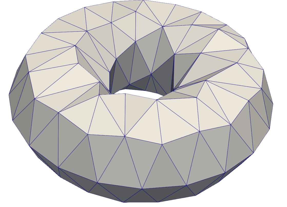
(a) $\mathcal{M}_{h}$

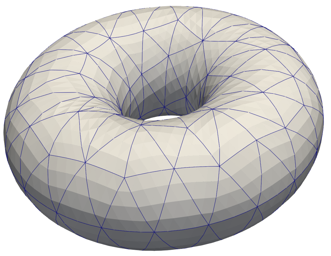
(b) $\mathcal{M}_{h}^{4}$

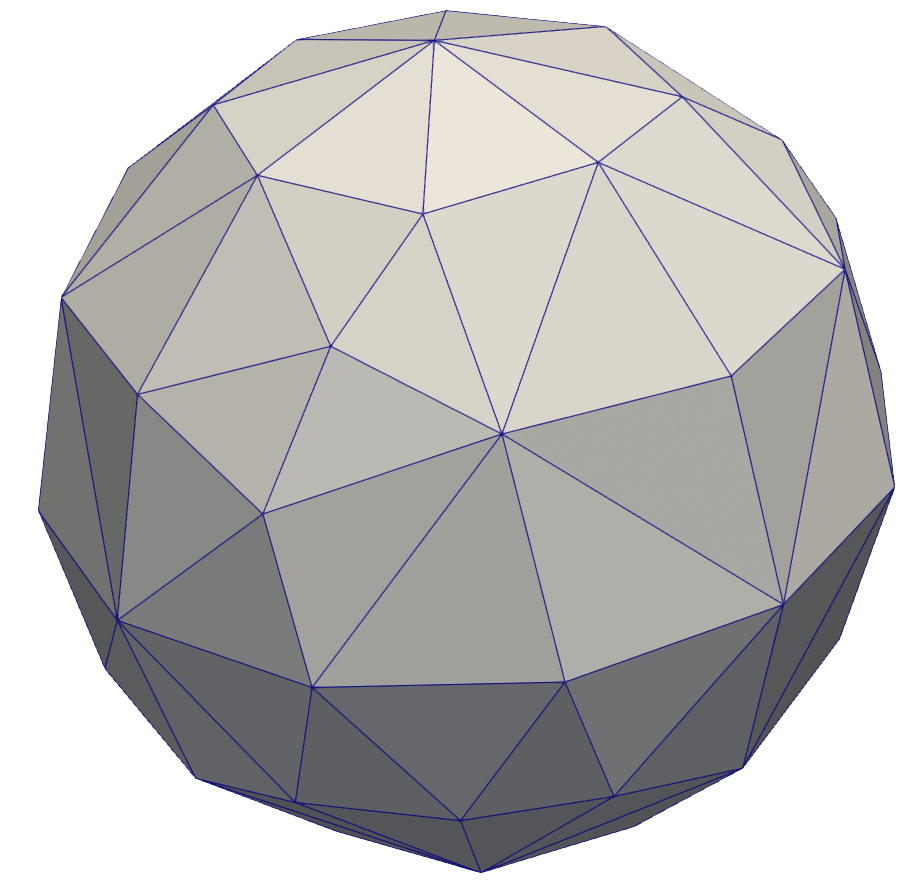
(c) $\mathcal{M}_{h}$

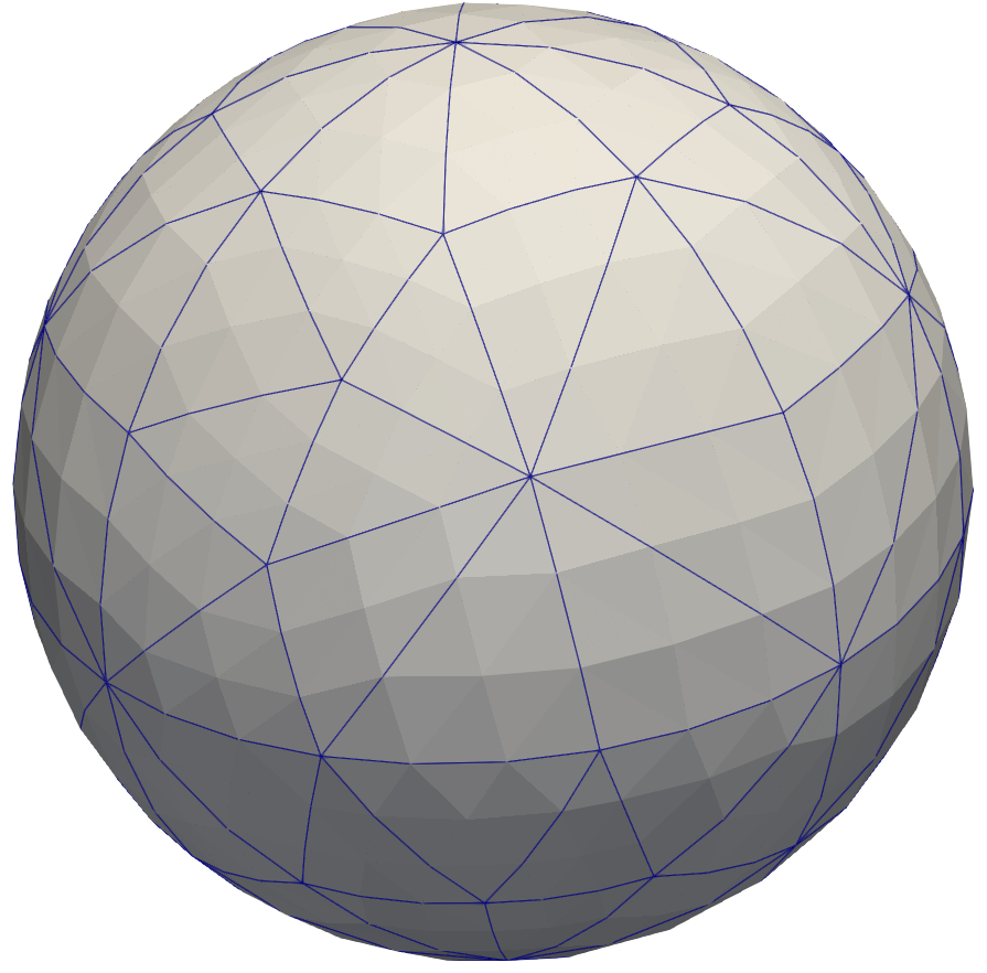
(d) $\mathcal{M}_{h}^{3}$

Figure 3: Lagrange parametrization for a torus and a sphere using equidistant nodes on vertices and edges.

3 Accuracy of Integration

In this section, we will prove our main theorem about the accuracy of integration when replacing $\mathcal{M}$ by its $k-$th order polygonal approximation $\mathcal{M}_{h}^{k}$ and show that symmetric triangles of the mesh combined with even-degree polynomials improve global errors. This motivates the following definition.

Figure 4: Illustration of bisection refinement and a duo of symmetric triangles obtained from the triangulation $\mathcal{T}^{1}_{h}$.

Definition 3.1 (symmetric triangles).

Given a collection of triangles $\mathcal{T}^{1}_{h}$ [Rup95], a pair of congruent triangles $T_{\mathbf{x}_{1},\mathbf{x}_{2},\mathbf{x}_{3}}$, $T_{\mathbf{x}_{1},\mathbf{x}_{4},\mathbf{x}_{5}}\in\mathcal{T}^{1}_{h}$ as in Fig. (4) are called symmetric with respect to their common vertex $\mathbf{x}_{1}$, if they satisfy the following property

$$\left(\mathbf{x}_{3}-\mathbf{x}_{1}\right)=-\left(\mathbf{x}_{5}-\mathbf{x}_{1}\right),\quad\left(\mathbf{x}_{2}-\mathbf{x}_{1}\right)=-\left(\mathbf{x}_{4}-\mathbf{x}_{1}\right).$$ (3.1)

Traditionally, the specific technique employed for triangulation refinement of a triangulation mesh $\mathcal{T}^{1}_{h}$ is often regarded as unimportant, provided that the grid size $h\longrightarrow 0$ as $n\longrightarrow\infty$. However, a more intricate picture emerges when the influence of integration process is taken into account. The choice of the appropriate type of triangulation can potentially result in a serendipitous cancellation of errors. Now, when examining a conforming triangulation $\mathcal{T}^{1}_{h}$, we refine each triangle $T\in\mathcal{T}^{1}_{h}$ into four smaller triangles using bisection refinement, which involves connecting the midpoints of its edges with straight lines. The new elements are all congruent, and they are similar to $T$. Repeating the bisection refinement $m-$ times, the total number of triangles at that level will be approximately $\mathcal{O}(2^{2m})$. An advantage of this form of refinement is that each set of mesh points contains those mesh points at the preceding level. During this refinement procedure, we obtain different triangular elements in size. For example, in Fig.4, you can observe three distinct triangular elements of varying sizes.

Consider $\mathcal{C}_{m},\,m\in\mathbb{N}$ as the set of triangles with equal size within $T\in\mathcal{T}^{1}_{h}$ at the $m$-th refinement level, and let $n_{m}$ represent the number of triangles in this set, then we can write

$$\mathcal{C}_{m}=\bigcup_{i=1}^{n_{m}}\{T^{i}_{h(\frac{1}{2})^{m}}\},\,\text{where}\,h=\mathrm{diam}(T).$$

For example, from the illustration in Fig. 4, we have

$$\mathcal{C}_{0}=T,\;\mathcal{C}_{1}=\bigcup_{i=1}^{n_{1}}\{T^{i}_{(\frac{h}{2})}\},\;\mathcal{C}_{2}=\bigcup_{i=1}^{n_{2}}\{T^{i}_{h(\frac{1}{2})^{2}}\},\;\mathcal{C}_{3}=\bigcup_{i=1}^{n_{3}}\{T^{i}_{h(\frac{1}{2})^{3}}\},\;\mathcal{C}_{4}=\bigcup_{i=1}^{n_{4}}\{T^{i}_{h(\frac{1}{2})^{4}}\}.\,$$

Observe that during each bisection refinement step, at least two triangles fail to meet the Definition 3.1. As an illustration, these triangles can be discerned based on their blue shading in Fig. 4. As a result, the density of symmetric pairs of triangles within $T\in\mathcal{T}^{1}_{h}$ after the $m$-th refinement level is $\mathcal{O}\left(\tilde{n}_{m}\right)$ while the remaining triangles exhibit a density of $\mathcal{O}\left(\sqrt{\tilde{n}_{m}}\right)$. Here, $\tilde{n}_{m}$ denotes the total number of triangles within $T\in\mathcal{T}^{1}_{h}$ after the $m$-th refinement.

Remark 3.2 (symmetric triangulation).

Any (smoothed closed) surface triangulation mesh that has undergone the refinement process previously described will be referred to as a symmetric triangulation.

In light of these facts, we state the main theorem of this article, showing that even degree approximation is superior to odd degree approximation for symmetric triangulations.

Theorem 3.3.

Let $\mathcal{M}$ be a smooth closed embedded hypersurface and $f\in\mathbf{C}^{k+2}\left(\mathcal{M},\mathbb{R}\right)$. Consider a piecewise linear triangulation $\mathcal{M}_{h}$ with mesh size $h$ of the smooth surface having vertices lie on $\mathcal{M}$ and let $\mathcal{M}^{k}_{h}$ be the $k-$th order approximation of the smooth surface constructed using local fittings of $\pi\in\mathbf{C}^{k+3}\left(\mathcal{M}_{h},\mathbb{R}^{3}\right)$. Consider a symmetric triangulation, consisting of $\mathcal{O}\left(n\right)=\mathcal{O}\left(h^{-2}\right)$ symmetric triangles, whereas the number of non-symmetric triangles is bounded by $\mathcal{O}\left(\sqrt{n}\right)=\mathcal{O}\left(h^{-1}\right)$. Then

$$\left|\int_{\mathcal{M}}f\,dS-\int_{\mathcal{M}^{k}_{h}}Q_{f,k}\,dS\right|\leq\begin{cases}Ch^{k+2},&k\equiv 0\ (\textrm{mod}\ 2)\\ Ch^{k+1},&k\equiv 1\ (\textrm{mod}\ 2),\end{cases}$$ (3.2)

where $Q_{f,k}:\mathcal{M}^{k}_{h}\rightarrow\mathbb{R}$ is a $k-$th order polynomial approximating the integrand $f$.

As we approach the proof of Theorem 3.3, we need three lemmata.

Lemma 3.4.

Let $T$ be a triangle in $\mathcal{T}^{1}_{h}$ and assume that $\psi\in\mathbf{C}^{k+1}\left(T\right)$ and $k\geq 0$, then we have

$$\left\lVert\psi-Q_{\psi,k}\right\rVert_{L^{\infty}\left(T\right)}\leq ch^{k+1}\max^{l,p,q\geq 0}_{l+p+q=k+1}\max_{\left(x,y,z\right)\in T}\Big{|}\frac{\partial^{k+1}\psi\left(x,y,z\right)}{\partial x^{l}\partial y^{p}\partial z^{q}}\Big{|}$$ (3.3)

with $h=diam(T)$. The constant $c$ depends on $k$, but it is independent of both $\psi$ and $T$.

Proof.

In order to prove this lemma, we will use Taylor’s formula in several variables. Let’s denote with $\alpha=\left(\alpha_{1},\alpha_{2}\right)$, where $|\alpha|=|\alpha_{1}|+|\alpha_{2}|$, $h:=\left(h_{1},h_{2}\right)=\left(s-0,t-0\right)$ and $\partial_{\alpha_{1}}=\partial_{s},\,\partial_{\alpha_{2}}=\partial_{t}.$
As a first step, let’s consider the $k-$ order interpolation of the map $\psi$

$$Q_{\psi,k}\left(\hat{p}\right):=\sum_{i=1}^{N\left(2,n\right)}p_{i}\mathcal{L}_{i}^{k}\left(\hat{p}\right).$$

Using Taylor’s formula for $\psi$ around the point $\left(0,0\right)$ we obtain:

$$\psi\left(\hat{p}\right)=\sum_{|\alpha|=k}\Big{(}\frac{\partial^{\alpha}}{\alpha!}\psi\left(0\right)h^{\alpha}\Big{)}+\frac{1}{k!}\int_{0}^{1}(1-\mu)^{k}\frac{d^{k+1}\psi\left(s\mu,t\mu\right)}{d^{k+1}\mu}d\mu.$$ (3.4)

Let us denote $H\left(\hat{p}\right)=\frac{1}{k!}\int_{0}^{1}(1-\mu)^{k}\frac{d^{k+1}\psi\left(s\mu,t\mu\right)}{d^{k+1}\mu}d\mu$, by interpolating each term in the Eq. (3.4) using a polynomial of order $k$ and using the fact that the interpolation of the first term is exact because it is a polynomial of degree $\leq k$, namely

$$\mathcal{I}_{k}\sum_{|\alpha|=k}\Big{(}\frac{\partial^{\alpha}}{\alpha!}\psi\left(0\right)h^{\alpha}\Big{)}=\sum_{|\alpha|=k}\Big{(}\frac{\partial^{\alpha}}{\alpha!}\psi\left(0\right)h^{\alpha}\Big{)},$$ (3.5)

we obtain

$$Q_{\psi,k}\left(\hat{p}\right)=\sum_{|\alpha|=k}\Big{(}\frac{\partial^{\alpha}}{\alpha!}\psi\left(0\right)h^{\alpha}\Big{)}+\sum_{i=1}^{N\left(2,n\right)}H\left(\hat{p}_{i}\right)\mathcal{L}_{i}^{k}\left(\hat{p}\right).$$ (3.6)

Subtracting Eq.(3.6) from Eq.(3.4), we have

$$\psi\left(\hat{p}\right)-Q_{\psi,k}\left(\hat{p}\right)=H\left(\hat{p}\right)-\sum_{i=1}^{N\left(2,n\right)}H\left(\hat{p}_{i}\right)\mathcal{L}_{i}^{k}\left(\hat{p}\right).$$ (3.7)

The right hand side of Eq.(3.7) can be written

$$H\left(\hat{p}\right)-\sum_{i=1}^{N\left(2,n\right)}H\left(\hat{p}_{i}\right)\mathcal{L}_{i}^{k}\left(\hat{p}\right)=\frac{1}{k!}\int_{0}^{1}(1-\mu)^{k}E\left(\mu;s,t\right)d\mu,$$ (3.8)

where $E\left(\mu;s,t\right)$ has the following form

$$E\left(\mu;s,t\right):=\frac{d^{k+1}\psi\left(s\mu,t\mu\right)}{d^{k+1}\mu}-\sum_{i=1}^{N\left(2,n\right)}\mathcal{L}_{i}^{k}\left(\hat{p}\right)\frac{d^{k+1}\psi\left(s_{i}\mu,t_{i}\mu\right)}{d^{k+1}\mu}.$$ (3.9)

It is important to note that the left-hand side of Eq. (3.7) is affected by the behavior of the term $E\left(\mu;s,t\right)$, which itself is influenced by $\frac{d^{k+1}\psi\left(s\mu,t\mu\right)}{d^{k+1}\mu}$. For $k=0$, we have

$$\max_{0\leq\mu\leq 1,\,\hat{p}\in\sigma}\bigg{|}\frac{d\psi\left(s\mu,t\mu\right)}{d\mu}\bigg{|}\leq ch\max\biggl{\{}\left\lVert\frac{\partial\psi}{\partial x}\right\rVert_{L^{\infty}},\left\lVert\frac{\partial\psi}{\partial y}\right\rVert_{L^{\infty}},\left\lVert\frac{\partial\psi}{\partial z}\right\rVert_{L^{\infty}}\biggr{\}},$$ (3.10)

where

$$\left\lVert\frac{\partial\psi}{\partial x}\right\rVert_{L^{\infty}}:=\max_{\left(x,y,z\right)\in T}\bigg{|}\frac{\partial\psi}{\partial x}\bigg{|}$$

and analogously for $\frac{\partial\psi}{\partial y},\,\frac{\partial\psi}{\partial z}$. Following the same line of reasoning with the higher-order derivatives of $\psi$, we obtain

$$\max_{0\leq\mu\leq 1,\,\hat{p}\in\sigma}\bigg{|}\frac{d^{k+1}\psi\left(s\mu,t\mu\right)}{d^{k+1}\mu}\bigg{|}\leq ch^{k+1}\max\biggl{\{}\left\lVert\frac{\partial\psi}{\partial x}\right\rVert_{L^{\infty}},\left\lVert\frac{\partial\psi}{\partial y}\right\rVert_{L^{\infty}},\left\lVert\frac{\partial\psi}{\partial z}\right\rVert_{L^{\infty}}\biggr{\}}.$$ (3.11)

Using (3.8), yields

$$H\left(\hat{p}\right)-\sum_{i=1}^{N\left(2,n\right)}H\left(\hat{p}_{i}\right)\mathcal{L}_{i}^{k}\left(\hat{p}\right)=\mathcal{O}\left(h^{k+1}\right).$$ (3.12)

Combining Eq. (3.7) with Eq. (3.12), yields Eq. (3.3). ∎

Next, we recall the following Lemma.

Lemma 3.5 ([Chi93]).

Let $k$ be an even integer. Let $\psi\left(\hat{p}\right)\in\mathcal{P}_{k+1}$ be a polynomial of degree $k+1$ on $\sigma$, and let $Q_{\psi,k}\left(\hat{p}\right)$ be its interpolant of degree $k$. Then, for each $\hat{p}\in\sigma$

$$\int_{\sigma}\partial_{s}\left(\psi\left(\hat{p}\right)-Q_{\psi,k}\left(\hat{p}\right)\right)dsdt=0,\quad\int_{\sigma}\partial_{t}\left(\psi\left(\hat{p}\right)-Q_{\psi,k}\left(\hat{p}\right)\right)dsdt=0.$$ (3.13)

Lemma 3.6.

Let $\mathcal{M}$ be a smooth closed hypersurface and consider a piecewise linear triangulation $\mathcal{M}_{h}$ with mesh size $h$ of the smooth surface $\mathcal{M}$ and let $\mathcal{M}^{k}_{h}$ be the $k-$th order approximation of the smooth surface constructed using local fittings of $\pi\in\mathbf{C}^{k+3}\left(\mathcal{M}_{h},\mathbb{R}^{3}\right)$. Consider a symmetric triangulation, consisting of $\mathcal{O}\left(n\right)=\mathcal{O}\left(h^{-2}\right)$ symmetric triangles, whereas the number of non-symmetric triangles is bounded by $\mathcal{O}\left(\sqrt{n}\right)=\mathcal{O}\left(h^{-1}\right)$. Then

$$\left|\int_{\mathcal{M}}dS-\int_{\mathcal{M}^{k}_{h}}dS\right|\leq\begin{cases}Ch^{k+1},&k\equiv 1\ (\textrm{mod}\ 2)\\ Ch^{k+2},&k\equiv 0\ (\textrm{mod}\ 2).\end{cases}$$ (3.14)

Proof.

First, let us write every term in Eq. (3.14) over a reference simplex

$$\int_{\mathcal{M}}dS=\sum_{i=1}^{n}\int_{\sigma}g_{i}dsdt,\quad\int_{\mathcal{M}^{k}_{h}}dS=\sum_{i=1}^{n}\int_{\sigma}\tilde{g}_{i}dsdt.$$ (3.15)

In the same manner, as in Lemma 3.4, we obtain

$$\psi\left(\hat{p}\right)-Q_{\psi,k}\left(\hat{p}\right)=\mathcal{R}_{k+1}+\mathcal{R}_{k+2}+\mathcal{O}\left(h^{k+3}\right),$$ (3.16)

where

$$\mathcal{R}_{k+1}:=\sum_{|\alpha|=k+1}\Big{(}\frac{\partial^{\alpha}}{\alpha!}\psi\left(0\right)h^{\alpha}-\sum_{i=1}^{N\left(2,n\right)}h^{\alpha}\frac{\partial^{\alpha}}{\alpha!}\psi\left(0\right)\mathcal{L}_{i}^{k}\left(\hat{p}\right)\Big{)}$$

$$\mathcal{R}_{k+2}:=\sum_{|\alpha|=k+2}\Big{(}\frac{\partial^{\alpha}}{\alpha!}\psi\left(0\right)h^{\alpha}-\sum_{i=1}^{N\left(2,n\right)}h^{\alpha}\frac{\partial^{\alpha}}{\alpha!}\psi\left(0\right)\mathcal{L}_{i}^{k}\left(\hat{p}\right)\Big{)}.$$

Analogously, an expansion can be given for the errors in the partial derivatives of $\partial_{\alpha_{1}}\psi\left(\hat{p}\right),\,\partial_{\alpha_{2}}\psi\left(\hat{p}\right)$, amounting to apply the derivative on (3.16). Therefore, we have

$$\partial_{\alpha_{1}}\psi\left(\hat{p}\right)-\partial_{\alpha_{1}}Q_{\psi,k}\left(\hat{p}\right)=\partial_{\alpha_{1}}\mathcal{R}_{k+1}+\partial_{\alpha_{1}}\mathcal{R}_{k+2}+\mathcal{O}\left(h^{k+2}\right)$$ (3.17)

$$\partial_{\alpha_{2}}\psi\left(\hat{p}\right)-\partial_{\alpha_{2}}Q_{\psi,k}\left(\hat{p}\right)=\partial_{\alpha_{2}}\mathcal{R}_{k+1}+\partial_{\alpha_{2}}\mathcal{R}_{k+2}+\mathcal{O}\left(h^{k+2}\right).$$ (3.18)

Using Taylor’s theorem and expanding about $\left(s=0,t=0\right)$, we obtain

$$g_{i}-\tilde{g}_{i} :=\sqrt{\det(J^{T}J)}-\sqrt{\det(\tilde{J}^{T}\tilde{J})}$$ (3.19)

$$=\mathcal{E}\left(h^{k+2};\left(\mathbf{x}_{k}-\mathbf{x}_{j}\right),\left(\mathbf{x}_{\ell}-\mathbf{x}_{j}\right)\right)+\mathcal{E}\left(h^{k+3};\left(\mathbf{x}_{k}-\mathbf{x}_{j}\right),\left(\mathbf{x}_{\ell}-\mathbf{x}_{j}\right)\right)+\mathcal{O}\left(h^{k+4}\right),$$

where $\mathcal{E}\left(h^{k+2};\left(\mathbf{x}_{k}-\mathbf{x}_{j}\right),\left(\mathbf{x}_{\ell}-\mathbf{x}_{j}\right)\right)$ and $\mathcal{E}\left(h^{k+3};\left(\mathbf{x}_{k}-\mathbf{x}_{j}\right),\left(\mathbf{x}_{\ell}-\mathbf{x}_{j}\right)\right)$, describes the collection of terms with order $k+2,k+3$ in $h$, whose coefficients are combinations of the vertices of triangles with appropriate indices $j,\,\ell$, and $k$. For example for a triangle $T_{\mathbf{x}_{1},\mathbf{x}_{2},\mathbf{x}_{3}}$ the coefficients are combination of $\left(\mathbf{x}_{3}-\mathbf{x}_{1}\right)$ and $\left(\mathbf{x}_{2}-\mathbf{x}_{1}\right)$ both for $\mathcal{E}\left(k+2\right)$ and $\mathcal{E}\left(k+3\right)$. From above computation we see that $\lvert g_{i}-\tilde{g}_{i}\lvert$ is at least of order $\mathcal{O}\left(h^{k+2}\right)$, confirming also the result obtained in ([RWJG12], Theorem 7). However, this result can be further improved assuming that the triangulation mesh comprises symmetric triangles. Thus, integrating Eq. (3.19) over a reference simplex, we have

$$\int_{\sigma}\big{(}g_{i}-\tilde{g}_{i}\big{)}dsdt=\int_{\sigma}\mathcal{E}\left(k+2\right)dsdt+\int_{\sigma}\mathcal{E}\left(k+3\right)dsdt+\mathcal{O}\left(h^{k+4}\right).$$ (3.20)

Now if $k$ is odd, yields

$$\int_{\sigma}\mathcal{E}\left(k+2\right)dsdt\neq 0$$

then, the left hand side of the Eq. (3.20) is at least of order $\mathcal{O}\left(h^{k+2}\right)$ for every $T\in\mathcal{T}^{1}_{h}$. Writing Eq. (3.20) with respect to a pair of symmetric triangles $T_{\mathbf{x}_{1},\mathbf{x}_{2},\mathbf{x}_{3}}$ and $T_{\mathbf{x}_{1},\mathbf{x}_{4},\mathbf{x}_{5}}$, we obtain

$$\left.\int_{\sigma}\big{(}g_{i}-\tilde{g}_{i}\big{)}dsdt\right|_{T_{\mathbf{x}_{1},\mathbf{x}_{2},\mathbf{x}_{3}}}=\int_{\sigma}\mathcal{E}\left(k+2\right)dsdt+\int_{\sigma}\mathcal{E}\left(k+3\right)dsdt+\mathcal{O}\left(h^{k+4}\right)$$ (3.21)

$$\left.\int_{\sigma}\big{(}g_{i}-\tilde{g}_{i}\big{)}dsdt\right|_{T_{\mathbf{x}_{1},\mathbf{x}_{4},\mathbf{x}_{5}}}=\int_{\sigma}\mathcal{E}\left(k+2\right)dsdt+\int_{\sigma}\mathcal{E}\left(k+3\right)dsdt+\mathcal{O}\left(h^{k+4}\right).$$ (3.22)

From Eq. (3.21) and Eq. (3.22), we have the following

$$\int_{\sigma}\big{(}g_{i}-\tilde{g}_{i}\big{)}dsdt=\int_{\sigma}\mathcal{E}\left(k+3\right)dsdt+\mathcal{O}\left(h^{k+4}\right).$$ (3.23)

This is due to the fact that the first right hand side integrand of the Eq. (3.21) and Eq. (3.22), are the collection of terms which are of order $k+2$ in $h$, where the coefficients are the combination of the vertices of triangles, thus each integrand is an odd function. In general for a triangle $T_{\mathbf{x}_{1},\mathbf{x}_{2},\mathbf{x}_{3}}$ we may write:

$$\mathcal{E}\left(h^{k+2};-\left(\mathbf{x}_{3}-\mathbf{x}_{1}\right),-\left(\mathbf{x}_{2}-\mathbf{x}_{1}\right)\right)=-\mathcal{E}\left(h^{k+2};\left(\mathbf{x}_{3}-\mathbf{x}_{1}\right),\left(\mathbf{x}_{2}-\mathbf{x}_{1}\right)\right).$$ (3.24)

In the same manner for $T_{\mathbf{x}_{1},\mathbf{x}_{4},\mathbf{x}_{5}}$

$$\mathcal{E}\left(h^{k+2};-\left(\mathbf{x}_{4}-\mathbf{x}_{1}\right),-\left(\mathbf{x}_{5}-\mathbf{x}_{1}\right)\right)=-\mathcal{E}\left(h^{k+2};\left(\mathbf{x}_{4}-\mathbf{x}_{1}\right),\left(\mathbf{x}_{5}-\mathbf{x}_{1}\right)\right).$$ (3.25)

Using the property (3.1), Eq. (3.24) and Eq. (3.25), we obtain

$$\mathcal{E}\left(h^{k+2};\left(\mathbf{x}_{3}-\mathbf{x}_{1}\right),\left(\mathbf{x}_{2}-\mathbf{x}_{1}\right)\right)+\mathcal{E}\left(h^{k+2};\left(\mathbf{x}_{4}-\mathbf{x}_{1}\right),\left(\mathbf{x}_{5}-\mathbf{x}_{1}\right)\right)=0.$$

The first part of inequality(3.14) is obtained by leveraging the fact that the number of symmetric triangles in the mesh $\mathcal{M}_{h}$ is of order $\mathcal{O}\left(n\right)=\mathcal{O}\left(h^{-2}\right)$, while the number of non-symmetric triangles is bounded by $\mathcal{O}\left(\sqrt{n}\right)=\mathcal{O}\left(h^{-1}\right)$, in combination with Eq. (3.20) and Eq. (3.23).

At this point, we notice that if $k$ is even, then

$$\int_{\sigma}\mathcal{E}\left(k+2\right)dsdt=0.$$

This is due to the Lemma 3.5 because $\mathcal{E}\left(k+2\right)$ represents errors when integrating a polynomial of order $k+1$. Thus, we have

$$\int_{\sigma}\big{(}g_{i}-\tilde{g}_{i}\big{)}dsdt=\int_{\sigma}\mathcal{E}\left(k+3\right)dsdt+\mathcal{O}\left(h^{k+4}\right).$$ (3.26)

Again, writing Eq. (3.26) with respect to a pair of symmetric triangles, we obtain $T_{\mathbf{x}_{1},\mathbf{x}_{2},\mathbf{x}_{3}}$ and $T_{\mathbf{x}_{1},\mathbf{x}_{4},\mathbf{x}_{5}}$

$$\left.\int_{\sigma}\big{(}g_{i}-\tilde{g}_{i}\big{)}dsdt\right|_{T_{\mathbf{x}_{1},\mathbf{x}_{2},\mathbf{x}_{3}}}=\int_{\sigma}\mathcal{E}\left(k+3\right)dsdt+\mathcal{O}\left(h^{k+4}\right)$$ (3.27)

$$\left.\int_{\sigma}\big{(}g_{i}-\tilde{g}_{i}\big{)}dsdt\right|_{T_{\mathbf{x}_{1},\mathbf{x}_{4},\mathbf{x}_{5}}}=\int_{\sigma}\mathcal{E}\left(k+3\right)dsdt+\mathcal{O}\left(h^{k+4}\right).$$ (3.28)

Now, if $k$ is even and triangles are pairwise symmetric then the error contributed is

$$\int_{\sigma}\big{(}g_{i}-\tilde{g}_{i}\big{)}dsdt=\mathcal{O}\left(h^{k+4}\right).$$ (3.29)

This is attributed to the fact that for $k$ even, the following holds true.

$$\mathcal{E}\left(h^{k+3};\left(\mathbf{x}_{3}-\mathbf{x}_{1}\right),\left(\mathbf{x}_{2}-\mathbf{x}_{1}\right)\right)+\mathcal{E}\left(h^{k+3};\left(\mathbf{x}_{4}-\mathbf{x}_{1}\right),\left(\mathbf{x}_{5}-\mathbf{x}_{1}\right)\right)=0.$$

As in the odd case, combining Eq. (3.26) and Eq. (3.29), it yields the second part of inequality(3.14). ∎

We can now prove Theorem 3.3

Poof of theorem 3.3.

As in Lemma 3.6, expanding the function $f$ using Taylor’s formula around the point $\left(0,0\right)$, yields

$$f\left(\psi\left(\hat{p}\right)\right)-Q_{f,k}\left(\psi\left(\hat{p}\right)\right)=\mathcal{R}_{k+1}+\mathcal{O}\left(h^{k+2}\right),$$ (3.30)

where $\mathcal{R}_{k+1}$ has the form

$$\mathcal{R}_{k+1}:=\sum_{|\alpha|=k+1}\Big{(}\frac{\partial^{\alpha}}{\alpha!}f\left(0\right)h^{\alpha}-\sum_{i=1}^{N\left(2,n\right)}h^{\alpha}\frac{\partial^{\alpha}}{\alpha!}f\left(0\right)\mathcal{L}_{i}^{k}\left(\hat{p}\right)\Big{)}.$$

Integrate both side of the Eq. (3.30), we have

$$\int_{\sigma}\left(f\left(\psi\left(\hat{p}\right)\right)-Q_{f,k}\left(\psi\left(\hat{p}\right)\right)\right)g_{i}dsdt=\int_{\sigma}\mathcal{R}_{k+1}g_{i}dsdt+\mathcal{O}\left(h^{k+4}\right).$$ (3.31)

Using $\lvert g_{i}\lvert=\mathcal{O}\left(h^{2}\right)$, the integral term on the right hand side is at least of order $\mathcal{O}\left(h^{k+3}\right)$. If $k$ is even due to the presence of symmetric triangles the first term on the right-hand side integral is $0$, so we can compute the left-hand integral with an accuracy of order $\mathcal{O}\left(h^{k+4}\right)$, while for $k$ odd, we have the following

$$\int_{\sigma}\left(f\left(\psi\left(\hat{p}\right)\right)-Q_{f,k}\left(\psi\left(\hat{p}\right)\right)\right)g_{i}\,ds\,dt=\mathcal{O}\left(h^{k+3}\right).$$ (3.32)

Assume that $\mathcal{M}_{h}^{k}$ is composed of triangles $\tilde{T}^{k}$, i.e. $\mathcal{M}_{h}^{k}=\bigcup_{i=1}^{n}\tilde{T}^{k}_{i}$ and the smooth closed surface, parameterized using (1.1) $\mathcal{M}=\bigcup_{i=1}^{n}V_{i}$. Then

$$\int_{\mathcal{M}}fdS=\sum_{i=1}^{n}\int_{V_{i}}fdS,\quad\int_{\mathcal{M}^{k}_{h}}Q_{f,k}dS=\sum_{i=1}^{n}\int_{\tilde{T}_{i}^{k}}Q_{f,k}dS.$$ (3.33)

Let us rewrite Eq. (3.33) over a reference simplex where the quadrature rules are defined

$$\int_{\mathcal{M}}fdS=\sum_{i=1}^{n}\int_{\sigma}f\left(\psi\left(\hat{p}\right)\right)g_{i}dsdt,\quad\int_{\mathcal{M}^{k}_{h}}Q_{f,k}dS=\sum_{i=1}^{n}\int_{\sigma}Q_{f,k}\left(\psi\left(\hat{p}\right)\right)\tilde{g}_{i}dsdt.$$ (3.34)

By making use of Lemma 3.6, we have

$$\left|\int_{\mathcal{M}}fdS-\int_{\mathcal{M}^{k}_{h}}Q_{f,k}dS\right| \leq\left|\sum_{i=1}^{n}\int_{\sigma}\Big{(}f\left(\psi\left(\hat{p}\right)\right)g_{i}-Q_{f,k}\left(\psi\left(\hat{p}\right)\right)\tilde{g}_{i}\Big{)}dsdt\right|$$

$$\leq\sum_{i=1}^{n}\left|\int_{\sigma}\left(f\left(\psi\left(\hat{p}\right)\right)-Q_{f,k}\left(\psi\left(\hat{p}\right)\right)\right)g_{i}+Q_{f,k}\left(\psi\left(\hat{p}\right)\right)\left(g_{i}-\tilde{g}_{i}\right)dsdt\right|$$

$$\leq\sum_{i=1}^{n}\int_{\sigma}\lvert\left(f\left(\psi\left(\hat{p}\right)\right)-Q_{f,k}\left(\psi\left(\hat{p}\right)\right)\right)g_{i}\lvert dsdt$$

$$+\int_{\sigma}\lvert Q_{f,k}\left(\psi\left(\hat{p}\right)\right)\left(g_{i}-\tilde{g}_{i}\right)\lvert dsdt$$

$$\leq\left\{\begin{array}[]{cc}Ch^{k+2},&k\equiv 0\ (\textrm{mod}\ 2)\\ Ch^{k+1},&k\equiv 1\ (\textrm{mod}\ 2)\end{array}\right.$$

∎

For the last inequality, we have used Eq. (3.31) and Eq. (3.32).

4 Results and Discussion

In order to validate our findings, we developed tests employing the Gauss-Bonnet theorem [PPCT01],
[Spi99] for a series of classic smooth closed surfaces given by the following equations:

1. Ellipsoid  $\frac{x^{2}}{a^{2}}+\frac{y^{2}}{b^{2}}+\frac{z^{2}}{c^{2}}=1$, $a,b,c\in\mathbb{R}\setminus\{0\}$.

2. Torus  $(x^{2}+y^{2}+z^{2}+R^{2}-r^{2})^{2}-4R^{2}(x^{2}+y^{2})=0$,  $0<r<R\in\mathbb{R}.$

3. Sphere  $x^{2}+y^{2}+z^{2}=R^{2}$,  $R\in\mathbb{R}\setminus\{0\}$.

The analytic expressions for the Gaussian Curvature are

1. Ellipsoid  $K_{\mathrm{Gauss}}=\frac{1}{(abc)^{2}\left(\frac{x^{2}}{a^{4}}+\frac{y^{2}}{b^{4}}+\frac{z^{2}}{c^{4}}\right)^{2}}$, $a,b,c\in\mathbb{R}\setminus\{0\}$.

2. Torus  $K_{\mathrm{Gauss}}=\frac{\cos v}{r(R+r\cos v)}$, where we used toric coordinates:

   $$(x,y,z)=\big{(}(R+r\cos\theta)\cos\varphi,(R+r\cos\theta)\sin\varphi,r\sin\theta\big{)},\;\varphi,\theta\in[0,2\pi).$$

3. Sphere  $K_{\mathrm{Gauss}}=\frac{1}{R^{2}}$,  $R\in\mathbb{R}\setminus\{0\}$.

In all experiments we utilize the algorithm of Persson and Strang [PS04] to generate Delaunay triangulations serving as the initial $\mathcal{M}^{1}_{h}$ surface approximation and a Gaussian quadrature rule of $deg=12$ on each triangle, employing $32$ quadrature points [Dun85].

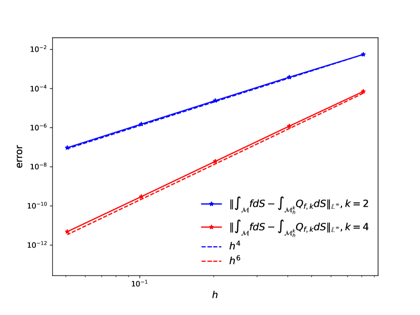
(a) Even order

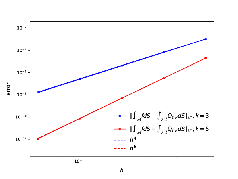
(b) Odd order

Figure 5: Relative errors by integrating the Gaussian curvature over the torus with radii $R=2,\,r=1$ with the ideal convergence lines $h^{n}$.

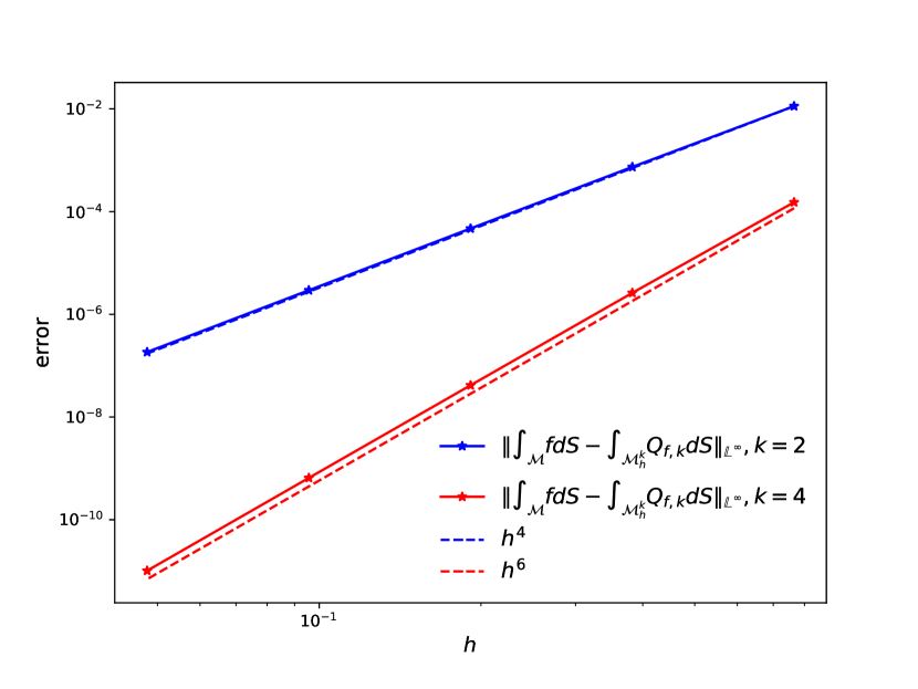
(a) Even order

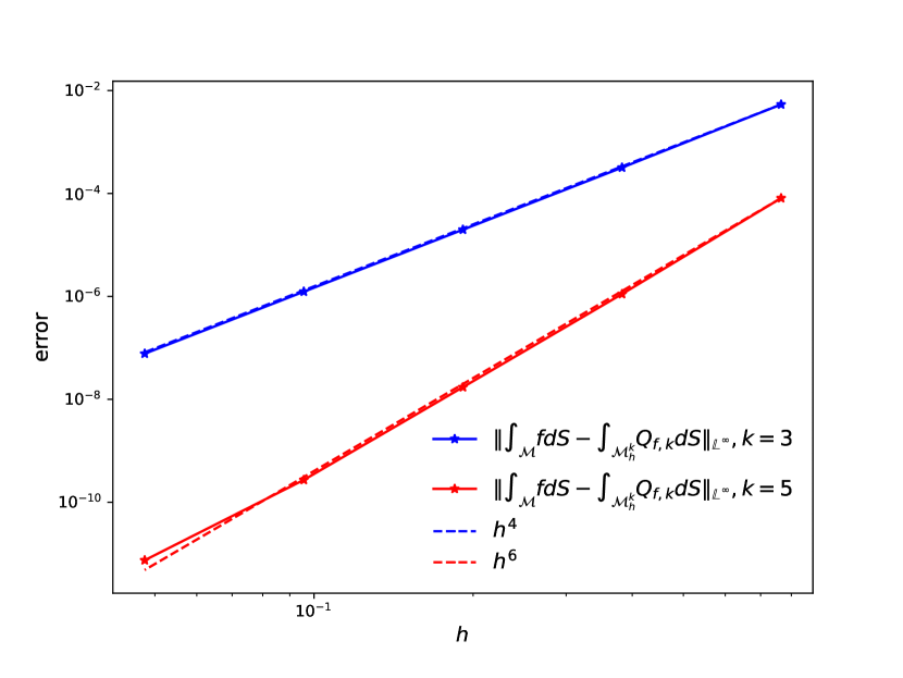
(b) Odd order

Figure 6: Relative errors by integrating the Gaussian curvature over the unit sphere with the ideal convergence lines $h^{n}$.

In Fig. 5 and Fig 6 we show the relative errors under mesh refinement. In order to calculate the relative error, we integrate the Gaussian curvature on the manifold and compare it with the predictions of the Gauss-Bonnet Theorem. The convergence rates shown on the plots coincide, confirming our theoretical results.

However, as can be seen from Fig. 7, the approach presented in [PS22] has some limitations, it runs into Runge’s phenomenon. This is due to the fact that the Lebesgue constant $\Lambda$ for the set of equidistant points grows exponentially [MS92].

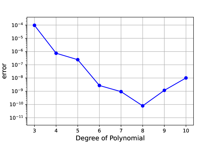
(a) torus with radii $R=2,r=1$

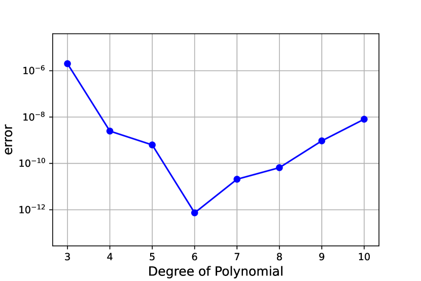
(b) ellipsoid with $a=b=1,c=0.6$.

Figure 7: Relative errors by integrating the Gaussian curvature over the torus and the ellipsoid using $N_{\Delta}=2528,\,N_{\Delta}=6152$ respectively.

To mitigate this effect, we propose an alternative approach. It is well known that under a proper map, the operations (e.g., interpolation, numerical differentiation, and quadrature) on a triangular element can be performed on the reference square. Below we will state and prove a theorem that we hope will pave the way for developing another powerful numerical integration method for closed surfaces. Prior to presenting the theorem, we first recall the modulus of continuity from [TIM63] (Chapter 3):

Let $\delta_{1}\geq 0$ and $\delta_{2}\geq 0$ be given. The modulus of continuity for a continuous function $f$ is represented by $\omega\left(f;\delta_{1},\delta_{2}\right)$, which is defined as:

$$\omega\left(f;\delta_{1},\delta_{2}\right)=\sup_{|x_{1}-x_{2}|\leq\delta_{1},\,x_{1},x_{2}\in[-1,1]}\quad\sup_{|y_{1}-y_{2}|\leq\delta_{2},\,y_{1},y_{2}\in[-1,1]}|f\left(x_{1},x_{2}\right)-f\left(y_{1},y_{2}\right)|.$$ (4.1)

The function $\omega\left(f;\delta_{1},\delta_{2}\right)$ is semi-additive, i.e,

$$\omega\left(\delta_{1}+\delta_{2},\lambda_{1}+\lambda_{2}\right)\leq\omega\left(\delta_{1}+\lambda_{1}\right)+\omega\left(\delta_{2}+\lambda_{2}\right).$$

To address Runge’s phenomenon, we propose the use of Chebyshev–Lobatto nodes as the interpolation points. Specifically, when working within a one-dimensional interpolation domain of $[-1,1]$, we define our new set of interpolation points as follows

$$\mathrm{Cheb}_{n}=\left\{\cos\Big{(}\frac{k\pi}{n}\Big{)}:0\leq k\leq n\right\}\,.$$

These points have a slow increase in the Lebesgue constant as $n\to\infty$, which can be estimated using the following expression

$$\Lambda(\mathrm{Cheb}_{n})=\frac{2}{\pi}\big{(}\log(n+1)+\gamma+\log(8/\pi)\big{)}+\mathcal{O}(1/n^{2})\,,$$ (4.2)

where $\gamma\approx 0.5772$ is the Euler-Mascheroni constant, see [Ber31, EZ66, Bru78]. To generate Chebyshev–Lobatto nodes on the square $[-1,1]^{2}$ we consider the tensorial product $\mathrm{Cheb}_{n}\times\mathrm{Cheb}_{n}$, yielding $\Lambda(\mathrm{Cheb}_{n}\times\mathrm{Cheb}_{n})=\Lambda(\mathrm{Cheb}_{n})^{2}$ [CM18]. Now, we can state the following result:

Theorem 4.1.

For $f\in\mathbf{C}^{k}\left([-1,1]^{2}\right)$, let $Q_{f,n}\left(x,y\right)$ be the interpolant of function $f$ in the Chebyshev–Lobatto nodes $\mathrm{Cheb}_{n}\times\mathrm{Cheb}_{n}$, we have the estimate

$$\left\lVert f\left(x,y\right)-Q_{f,n}\left(x,y\right)\right\rVert_{L^{\infty}\left([-1,1]^{2}\right)}\leq\tilde{C}\ln^{2}\left(n\right)n^{-k}\left(\omega\left(\partial_{x}^{k}f\left(x,y\right);\frac{1}{n},0\right)+\omega\left(\partial_{y}^{k}f\left(x,y\right);0,\frac{1}{n}\right)\right).$$ (4.3)

Remark 4.2.

Based on Theorem 4.1 in future work, we plan to incorporate recent advances in multivariate interpolation [HCHS17, HHCS18, HGM⁺20, HS18], providing a stable approach suppressing Runge’s phenomenon by interpolating the map $\psi$ in proper chosen, transformed Chebyshev-Lobatto nodes.

Poof of Theorem 4.1.

We consider the interpolation operator

$$\mathbf{I}_{[-1,1]^{2}}:\mathbf{C}^{0}\big{(}[-1,1]^{2},\mathbb{R}\big{)}\rightarrow\mathcal{P}_{2,n}$$

in the Chebyshev–Lobatto nodes $\mathrm{Cheb}_{n}\times\mathrm{Cheb}_{n}$, with $\mathcal{P}_{2,n}$ being the space of bivariate polynomials of maximum degree $n$. Its operator norm $\|\mathbf{I}_{[-1,1]^{2}}\|=\Lambda(\mathrm{Cheb}_{n})^{2}\in\mathcal{O}(\ln^{2})$ is given by the Lebesgue constant [CM18]. Let us denote with $Q_{f,n}^{*}\left(x,y\right)$ the best polynomial approximation of degree $n.$ The identity theorem for polynomials yields $Q_{f,n}^{*}\left(x,y\right)=\mathbf{I}_{[-1,1]^{2}}\left(Q_{f,n}^{*}\left(x,y\right)\right)$, by making use of Lemma 7.4 in [HGM⁺20], we have

$$\left\lVert f\left(x,y\right)-Q_{f,n}\left(x,y\right)\right\rVert_{L^{\infty}\left([-1,1]^{2}\right)}$$

$$\leq\left\lVert Q_{f,n}^{*}\left(x,y\right)-f\left(x,y\right)\right\rVert_{L^{\infty}\left([-1,1]^{2}\right)}+\left\lVert Q_{f,n}^{*}\left(x,y\right)-Q_{f,n}\left(x,y\right)\right\rVert_{L^{\infty}\left([-1,1]^{2}\right)}$$

$$\leq\left\lVert Q_{f,n}^{*}\left(x,y\right)-f\left(x,y\right)\right\rVert_{L^{\infty}\left([-1,1]^{2}\right)}+\left\lVert\mathbf{I}_{[-1,1]^{2}}\left(Q_{f,n}^{*}\left(x,y\right)-f\left(x,y\right)\right)\right\rVert_{L^{\infty}\left([-1,1]^{2}\right)}$$

$$\leq\left(1+C_{\Lambda}\ln^{2}\left(n\right)\right)\left\lVert f\left(x,y\right)-Q_{f,n}^{*}\left(x,y\right)\right\rVert_{L^{\infty}\left([-1,1]^{2}\right)}.$$ (4.4)

At this point, the multivariate version of Jackson’s inequality and semi-additivity of the modulus [TIM63], gives

$$\left\lVert f\left(x,y\right)-Q_{f,n}^{*}\left(x,y\right)\right\rVert_{L^{\infty}\left([-1,1]^{2}\right)} \leq C\left(2^{k}n^{-k}\omega\left(\partial_{x}^{k}f\left(x,y\right);\frac{2}{n},0\right)+2^{k}n^{-k}\omega\left(\partial_{y}^{k}f\left(x,y\right);0,\frac{2}{n}\right)\right)$$

$$\leq C2^{k+1}n^{-k}\left(\omega\left(\partial_{x}^{k}f\left(x,y\right);\frac{1}{n},0\right)+\omega\left(\partial_{y}^{k}f\left(x,y\right);0,\frac{1}{n}\right)\right).$$ (4.5)

Combining inequality (4.5) with (4.4), we obtain (4.3). ∎

In light of the multivariate extension of Jackson’s theorem [BBL02], we have the following result.

Corollary 4.3.

Let $f\in\mathbf{C}^{k}\left([-1,1]^{2}\right)$, we have the estimate

$$\left\lVert\partial_{x}f\left(x,y\right)-\partial_{x}Q_{f,n}\left(x,y\right)\right\rVert_{L^{\infty}\left([-1,1]^{2}\right)}\leq C\left(f;n\right)\ln^{2}\left(n\right)n^{-(k-1)}$$ (4.6)

and similarly

$$\left\lVert\partial_{y}f\left(x,y\right)-\partial_{y}Q_{f,n}\left(x,y\right)\right\rVert_{L^{\infty}\left([-1,1]^{2}\right)}\leq C\left(f;n\right)\ln^{2}\left(n\right)n^{-(k-1)},$$ (4.7)

where C is a suitable constant (with n), dependent on $f(x,y)$ and $k.$

Remark 4.4.

If $f\in\mathbf{C}^{k}\left([-1,1]^{2}\right)$ satisfy the Dini–Lipschitz criterion in the sense that

$$\lim_{n\longrightarrow\infty}\ln^{2}\left(n\right)\omega\left(f\left(x,y\right);\frac{1}{n},\frac{1}{n}\right)=0\,.$$

Then Eq. (4.3) guarantees uniform convergence

$$\lim_{n\longrightarrow\infty}\left\lVert f\left(x,y\right)-Q_{f,n}\left(x,y\right)\right\rVert_{L^{\infty}\left([-1,1]^{2}\right)}=0.$$

Additionally, it is easy to see that, for $f\in\mathbf{C}^{k}(T)$, we have

$$\left\lVert f\left(x,y\right)-Q_{f,n}\left(x,y\right)\right\rVert_{L^{\infty}\left(T\right)}\leq c\left\lVert f\left(x,y\right)-Q_{f,n}\left(x,y\right)\right\rVert_{L^{\infty}\left([-1,1]^{2}\right)}=\mathcal{O}\left(n^{-k}\right).$$ (4.8)

It is anticipated that with this initiative, we can develop an efficient numerical integration method for closed surfaces. This will be addressed in a forthcoming work.

Declaration of Competing Interest

The authors declare that they have no known competing financial interests or personal relationships that could have appeared to influence the work reported in this paper.

References

[BBL02]
Thomas Bagby, Len Bos, and Norman Levenberg.
Multivariate simultaneous approximation.
Constructive approximation, 18(4):569–577, 2002.
[Ber31]
Serge Bernstein.
Sur la limitation des valeurs d’un polynôme de degré n sur tout un segment par ses valeurs en points du segment.
Izv. Akad. Nauk SSSR, 7:1025–1050, 1931.
[Bru78]
L Brutman.
On the Lebesgue function for polynomial interpolation.
SIAM Journal on Numerical Analysis, 15(4):694–704, 1978.
[BV21]
Paul Breiding and Nick Vannieuwenhoven.
The condition number of riemannian approximation problems.
SIAM Journal on Optimization, 31(1):1049–1077, jan 2021.
[Chi93]
David Da-Kwun Chien.
Piecewise polynomial collocation for integral equations with a smooth kernel on surfaces in three dimensions.
The Journal of Integral Equations and Applications, 5:315–44, 1993.
[CM18]
Albert Cohen and Giovanni Migliorati.
Multivariate approximation in downward closed polynomial spaces.
In Contemporary Computational Mathematics-A celebration of the 80th birthday of Ian Sloan, pages 233–282. Springer, 2018.
[Dem09]
Alan Demlow.
Higher-order finite element methods and pointwise error estimates for elliptic problems on surfaces.
SIAM Journal on Numerical Analysis, 47(2):805–827, 2009.
[Dun85]
DA794241 Dunavant.
High degree efficient symmetrical Gaussian quadrature rules for the triangle.
International journal for numerical methods in engineering, 21(6):1129–1148, 1985.
[EZ66]
H Ehlich and K Zeller.
Auswertung der Normen von Interpolationsoperatoren.
Mathematische Annalen, 164(2):105–112, 1966.
[Geo98]
Kurt Georg.
Approximation of integrals for boundary element methods.
SIAM Journal on Scientific and Statistical Computing, 12, 08 1998.
[GR09]
Christophe Geuzaine and Jean-François Remacle.
Gmsh: A 3-d finite element mesh generator with built-in pre-and post-processing facilities.
International journal for numerical methods in engineering, 79(11):1309–1331, 2009.
[HCHS17]
M Hecht, Bevan L. Cheeseman, Karl B. Hoffmann, and Ivo F. Sbalzarini.
A quadratic-time algorithm for general multivariate polynomial interpolation.
arXiv preprint arXiv:1710.10846, 2017.
[HGM+20]
Michael Hecht, Krzysztof Gonciarz, Jannik Michelfeit, Vladimir Sivkin, and Ivo F Sbalzarini.
Multivariate interpolation in unisolvent nodes–lifting the curse of dimensionality.
arXiv preprint arXiv:2010.10824, 2020.
[HHCS18]
Michael Hecht, Karl B. Hoffmann, Bevan L Cheeseman, and Ivo F Sbalzarini.
Multivariate Newton interpolation.
arXiv preprint arXiv:1812.04256, 2018.
[HS18]
Michael Hecht and Ivo F. Sbalzarini.
Fast interpolation and Fourier transform in high-dimensional spaces.
In K. Arai, S. Kapoor, and R. Bhatia, editors, Intelligent Computing. Proc. 2018 IEEE Computing Conf., Vol. 2,, volume 857 of Advances in Intelligent Systems and Computing, pages 53–75, London, UK, 2018. Springer Nature.
[Lee13]
John M Lee.
Smooth manifolds.
In Introduction to smooth manifolds, pages 1–31. Springer, 2013.
[Lim88]
Elon L. Lima.
The jordan-brouwer separation theorem for smooth hypersurfaces.
The American Mathematical Monthly, 95(1):39–42, 1988.
[MS92]
T. M. Mills and Simon Jeffrey Smith.
The lebesgue constant for lagrange interpolation on equidistant nodes.
Numerische Mathematik, 61:111–115, 1992.
[PPCT01]
L.M.A. Pressley, A. Pressley, M. Chaplain, and J.F. Toland.
Elementary Differential Geometry.
Springer undergraduate mathematics series. Springer, 2001.
[PS04]
Per-Olof Persson and Gilbert Strang.
A simple mesh generator in matlab.
SIAM Review, 46(2):329–345, 2004.
[PS22]
Simon Praetorius and Florian Stenger.
Dune-curvedgrid - a dune module for surface parametrization.
Archive of Numerical Software, page Vol. 1 No. 1 (2022), 2022.
[Rup95]
J. Ruppert.
A delaunay refinement algorithm for quality 2-dimensional mesh generation.
Journal of Algorithms, 18(3):548–585, 1995.
[RWJG12]
Navamita Ray, Duo Wang, Xiangmin Jiao, and James Glimm.
High-order numerical integration over discrete surfaces.
SIAM Journal on Numerical Analysis, 50(6):3061–3083, 2012.
[Spi99]
M. Spivak.
A Comprehensive Introduction to Differential Geometry.
Number v. 1 in A Comprehensive Introduction to Differential Geometry. Publish or Perish, Incorporated, 1999.
[TIM63]
A. TIMAN.
Theory of Approximation of Functions of a Real Variable.
International Series of Monographs on Pure and Applied Mathematics. Pergamon, 1963.
[YQ09]
Pinghai Yang and Xiaoping Qian.
A general, accurate procedure for calculating molecular interaction force.
Journal of Colloid and Interface Science, 337(2):594–605, 2009.