Error estimates of the time-splitting methods for the nonlinear Schrödinger equation with semi-smooth nonlinearity

Abstract.

We establish error bounds of the Lie-Trotter time-splitting sine pseudospectral method for the nonlinear Schrödinger equation (NLSE) with semi-smooth nonlinearity $f(\rho)=\rho^{\sigma}$, where $\rho=|\psi|^{2}$ is the density with $\psi$ the wave function and $\sigma>0$ is the exponent of the semi-smooth nonlinearity. Under the assumption of $H^{2}$-solution of the NLSE, we prove error bounds at $O(\tau^{\frac{1}{2}+\sigma}+h^{1+2\sigma})$ and $O(\tau+h^{2})$ in $L^{2}$-norm for $0<\sigma\leq\frac{1}{2}$ and $\sigma\geq\frac{1}{2}$, respectively, and an error bound at $O(\tau^{\frac{1}{2}}+h)$ in $H^{1}$-norm for $\sigma\geq\frac{1}{2}$, where $h$ and $\tau$ are the mesh size and time step size, respectively. In addition, when $\frac{1}{2}<\sigma<1$ and under the assumption of $H^{3}$-solution of the NLSE, we show an error bound at $O(\tau^{\sigma}+h^{2\sigma})$ in $H^{1}$-norm. Two key ingredients are adopted in our proof: one is to adopt an unconditional $L^{2}$-stability of the numerical flow in order to avoid an a priori estimate of the numerical solution for the case of $0<\sigma\leq\frac{1}{2}$, and to establish an $l^{\infty}$-conditional $H^{1}$-stability to obtain the $l^{\infty}$-bound of the numerical solution by using the mathematical induction and the error estimates for the case of $\sigma\geq\frac{1}{2}$; and the other one is to introduce a regularization technique to avoid the singularity of the semi-smooth nonlinearity in obtaining improved local truncation errors. Finally, numerical results are reported to demonstrate our error bounds.

1. Introduction

In this paper, we consider the following nonlinear Schrödinger equation (NLSE)

(1.1) $$i\partial_{t}\psi(\mathbf{x},t)=-\Delta\psi(\mathbf{x},t)+V(\mathbf{x})\psi(\mathbf{x},t)+f(|\psi(\mathbf{x},t)|^{2})\psi(\mathbf{x},t),\quad\mathbf{x}\in\Omega,\quad t>0,$$

with the initial data

(1.2) $$\psi(\mathbf{x},0)=\psi_{0}(\mathbf{x}),\quad\mathbf{x}\in\overline{\Omega},$$

and the homogeneous Dirichlet boundary condition

(1.3) $$\psi(\mathbf{x},t)=0,\quad\mathbf{x}\in\partial\Omega,\quad t\geq 0,$$

where $t$ is time, $\mathbf{x}\in\mathbb{R}^{d}$ ($d=1,2,3$) is the spatial coordinate, $\psi:=\psi(\mathbf{x},t)$ is a complex-valued wave function, and $V:=V(\mathbf{x}):\Omega\rightarrow\mathbb{R}$ is a time-independent real-valued potential. Here $\Omega=\Pi_{i=1}^{d}(a_{i},b_{i})\subset\mathbb{R}^{d}$ is a bounded domain, and the nonlinearity is given as

(1.4) $$f(\rho)=\beta\rho^{\sigma},\quad\rho:=|\psi|^{2}\geq 0,$$

where $\beta\in\mathbb{R}$ is a given constant and $\sigma>0$ is the exponent of the nonlinearity. The NLSE Equation 1.1 conserves the mass

(1.5) $$M(\psi(\cdot,t))=\int_{\Omega}|\psi(\mathbf{x},t)|^{2}\mathrm{d}\mathbf{x}\equiv M(\psi_{0}),\quad t\geq 0,$$

and the energy

(1.6) $$E(\psi(\cdot,t)) =\int_{\Omega}\left[|\nabla\psi(\mathbf{x},t)|^{2}+V(\mathbf{x})|\psi(\mathbf{x},t)|^{2}+F(|\psi(\mathbf{x},t)|^{2})\right]\mathrm{d}\mathbf{x}$$

$$\equiv E(\psi_{0}),\quad t\geq 0,$$

where the interaction energy density $F(\rho)$ is given as

(1.7) $$F(\rho)=\int_{0}^{\rho}f(s)\mathrm{d}s=\frac{\beta}{\sigma+1}\rho^{\sigma+1},\quad\rho\geq 0.$$

When $\sigma=1$ in (1.4), i.e. $f(\rho)=\beta\rho$ and $F(\rho)=\frac{\beta}{2}\rho^{2}$, Equation 1.1 collapses to the well-known nonlinear Schrödinger equation with cubic nonlinearity (or smooth nonlinearity), also known as the Gross-Pitaevskii equation (GPE), which has been widely adopted for modeling and simulation in quantum mechanics, nonlinear optics, and Bose-Einstein condensation [6, 23, 44]. Arising from different physics applications, semi-smooth nonlinearity is introduced in the NLSE Equation 1.1, i.e. $\sigma$ is taken as a non-integer in (1.4). Typical examples include, in the Schrödinger-Poisson-X$\alpha$ model with $f(\rho)=-\alpha\rho^{1/d}(\alpha>0)$ [14, 16], i.e. $\sigma=\frac{1}{3}$ and $\sigma=\frac{1}{2}$ in three dimensions (3D) and two dimensions (2D), respectively; in the LHY correction (a next-order correction of the ground state energy proposed by Lee, Huang and Yang in 1957 [32]) for a beyond-mean-field term which is widely adopted in modeling and simulation for quantum droplets [29, 17, 4, 39, 27] with $f(\rho)=\rho^{3/2}$ in 3D, i.e. $\sigma=\frac{3}{2}$, $f(\rho)=\sqrt{\rho}$ in one dimension (1D), i.e. $\sigma=\frac{1}{2}$, and $f(\rho)=\rho\ln\rho$ in 2D; and in the mean field model for Bose-Fermi mixture [24, 18], with $f(\rho)=\rho^{2/3}$, i.e. $\sigma=\frac{2}{3}$. For all the aforementioned nonlinearities (actually for all $\sigma>0$ when $d=1,2,3$), the NLSE Equation 1.1 is well-posed in $H^{2}$ under suitable assumptions on $V$, e.g. $V\in L^{p}$ with $p\geq 1$ and $p>d/2$ [30, 19]. However, to our best knowledge, there is no guarantee of higher regularity to be propagated due to the low regularity of the semi-smooth nonlinearity, which is similar to the case of the logarithmic Schrödinger equation (LogSE) [9, 10, 11]. In fact, similar to the LogSE, the low regularity of the solution of the NLSE with semi-smooth nonlinearity is mainly due to the low regularity of the nonlinearity. We remark here that the potential $V$ could also be a source of low regularity of the solution, however, we will not consider the low regularity of $V$ in this paper but leave it as our future work.

For the cubic NLSE, i.e. $\sigma=1$, many accurate and efficient numerical methods have been proposed and analyzed in the last two decades, including the finite difference method [1, 7, 6, 3], the exponential wave integrator [8, 26, 20], the time-splitting method [13, 15, 33, 22, 6, 34, 3], the finite element method [2, 42, 45, 46, 25], etc. Recently, new low regularity integrators or resonance based Fourier integrators are designed and analyzed for the cubic NLSE with low regularity initial data since the important work by Ostermann and Schratz [36], followed by [31, 35, 41, 38, 37] and references therein for different dispersive partial differential equations. For all these numerical methods, optimal error bounds were rigorously established under different regularity assumptions of the cubic NLSE.

Most numerical methods for the cubic NLSE can be extended straightforwardly to solve the NLSE Equation 1.1 with non-integer $\sigma>0$, e.g. semi-smooth nonlinearity with $0<\sigma<1$, which is different from the NLSE with singular nonlinearity, where regularization may be needed [9, 10, 11, 12]. However, due to the low regularity of solution of the NLSE Equation 1.1 with semi-smooth nonlinearity and the low regularity of the semi-smooth nonlinearity (1.4) in the NLSE Equation 1.1 which causes order reduction in local truncation errors and results in difficulties in obtaining stability estimates, error analysis for different numerical methods applied to Equation 1.1 with non-integer $\sigma>0$ is a very subtle and challenging question! For example, first order temporal convergence of the finite difference method requires boundedness of the second-order time derivative, which roughly requires the exact solution to be in $H^{4}$, which is beyond the regularity property of the NLSE Equation 1.1 with semi-smooth nonlinearity. In fact, based on our numerical experiments with a smooth initial datum $\psi_{0}(x)=xe^{-x^{2}/2}$, it indicates that $\psi(\cdot,t)\not\in H^{4}$ for $t>0$ and $\sigma$ small! Since the time-splitting methods usually need lower regularity requirements on the exact solution than the finite difference methods, in this work, we consider the time-splitting method and in particular the first-order Lie-Trotter splitting method due to the low regularity of the semi-smooth nonlinearity and the low regularity of the exact solution of Equation 1.1.

Error estimates of the time-splitting methods with different orders for the cubic NLSE (i.e. $\sigma=1$) have been well understood and we refer the readers to [33, 22, 34, 3] and references therein. However, for the NLSE with non-integer $\sigma$, only limited results are established for the filtered Lie-Trotter splitting scheme which requires a strong CFL-type time step size restriction $\tau=O(h^{2})$. In [28], first order convergence in $L^{2}$-norm is established for $H^{2}$-solution and $\sigma\geq 1/2$. Then generalized in [21], half order convergence in $L^{2}$-norm is established for $H^{1}$-solution and $\sigma>0$. These convergence rates are optimal with respect to the regularity assumptions on the exact solution. However, there are still some questions related to error estimates to be addressed: (i) it is unclear whether higher convergence order can be obtained for $H^{2}$-solution when $0<\sigma<1/2$; (ii) their results are established for the filtered Lie-Trotter scheme, which is a semi-discretization scheme with a specific strong CFL-type time step size restriction, and it loses mass conservation and time symmetric property in the discretized level; and (iii) there is no optimal error estimate in $H^{1}$-norm, which is the natural norm of the NLSE.

The main aim of this paper is to establish error estimates of the time-splitting sine pseudospectral (TSSP) method Equation 2.13 for the NLSE Equation 1.1 with semi-smooth nonlinearity. We remark here that the TSSP is a fully discrete scheme and it preserves many good properties of the original NLSE in the discretized level, including mass conservation and time symmetry as well as dispersion relation. When $0<\sigma\leq\frac{1}{2}$, under the assumption of $H^{2}$-solution of the NLSE, we prove error bounds at $O(\tau^{\frac{1}{2}+\sigma}+h^{1+2\sigma})$ in $L^{2}$-norm without any CFL-type time step size restriction, which also fill the gap between the results in [28, 21]. When $\sigma\geq 1/2$, under the assumption of $H^{2}$-solution again, we prove error bounds at $O(\tau+h^{2})$ and $O(\tau^{\frac{1}{2}}+h)$ in $L^{2}$-norm and $H^{1}$-norm, respectively, with a very mild CFL-type time step size restriction, which generalize the result in [28] to the mass-conservative fully discrete scheme. In addition, when $\frac{1}{2}<\sigma<1$ and under the assumption of $H^{3}$-solution, we show a new error bound at $O(\tau^{\sigma}+h^{2\sigma})$ in $H^{1}$-norm.

The rest of the paper is organized as follows. In Section 2, we present the time-splitting sine pseudospectral (TSSP) method, introduce a local regularization for the semi-smooth nonlinearity to be used for obtaining improved local truncation errors and state our main results. Section 3 is devoted to error estimates of the TSSP method for $0<\sigma\leq 1/2$ and Section 4 is devoted to error estimates for $\sigma\geq 1/2$. Numerical results are reported in Section 5 to confirm the error estimates. Finally some conclusions are drawn in Section 6. Throughout the paper, we adopt the standard Sobolev spaces as well as the corresponding norms, and denote by $C$ a generic positive constant independent of the mesh size $h$, time step $\tau$, and by $C(\alpha)$ a generic positive constant depending on $\alpha$. The notation $A\lesssim B$ is used to represent that there exists a generic constant $C>0$, such that $|A|\leq CB$.

2. Numerical methods and main results

2.1. The TSSP method

We shall use the Lie-Trotter splitting method for the temporal discretization and use the sine pseudospectral method for the spatial discretization. The operator splitting technique is based on the decomposition of the flow of Equation 1.1

(2.1) $$\partial_{t}\psi=A(\psi)+B(\psi),$$

where

(2.2) $$A(\psi)=i\Delta\psi,\quad B(\psi)=B_{1}(\psi)+B_{2}(\psi):=-iV\psi-if(|\psi|^{2})\psi,$$

into two sub-problems. The first one is

(2.3) $$\left\{\begin{aligned} &\partial_{t}\psi(\mathbf{x},t)=A(\psi)=i\Delta\psi(\mathbf{x},t),\quad\mathbf{x}\in\Omega,\quad t>0,\\ &\psi(\mathbf{x},0)=\psi_{0}(\mathbf{x}),\quad\mathbf{x}\in\overline{\Omega},\end{aligned}\right.$$

which can be formally integrated exactly in time as

(2.4) $$\psi(\cdot,t)=e^{it\Delta}\psi_{0}(\cdot),\quad t\geq 0.$$

The second one is to solve

(2.5) $$\left\{\begin{aligned} &\partial_{t}\psi(\mathbf{x},t)=B(\psi)=-iV(\mathbf{x})\psi(\mathbf{x},t)-if(|\psi(\mathbf{x},t)|^{2})\psi(\mathbf{x},t),\quad\mathbf{x}\in\Omega,\ t>0,\\ &\psi(\mathbf{x},0)=\psi_{0}(\mathbf{x}),\quad\mathbf{x}\in\overline{\Omega},\end{aligned}\right.$$

which, by using the fact $|\psi(\mathbf{x},t)|=|\psi_{0}(\mathbf{x})|$ for $t\geq 0$, can be integrated exactly in time as

(2.6) $$\psi(\mathbf{x},t)=\Phi_{B}^{t}(\psi_{0}):=e^{-itV(\mathbf{x})}{\Phi_{B_{2}}^{t}(\psi_{0}(\mathbf{x}))},\quad\mathbf{x}\in\overline{\Omega},\quad t\geq 0,$$

where

(2.7) $$\quad{\Phi_{B_{2}}^{t}(z)}=ze^{-itf(|z|^{2})},\quad z\in\mathbb{C},\quad t\geq 0.$$

In fact, in the second subproblem Equation 2.5, the operator $B(\psi)=-i(V+f(|\psi_{0}|^{2}))\psi$ becomes a bounded linear operator.

Choose a time step size $\tau>0$, denote time steps as $t_{k}=k\tau$ for $k=0,1,...$, and let $\psi^{[k]}:=\psi^{[k]}(\mathbf{x})$ be the approximation of $\psi(\mathbf{x},t_{k})$ for $k\geq 0$. Then a first order semi-discretization of the NLSE Equation 1.1 via the Lie-Trotter splitting is given as:

(2.8) $$\psi^{[k+1]}=e^{i\tau\Delta}\Phi_{B}^{\tau}(\psi^{[k]}),$$

with $\psi^{[0]}(\mathbf{x})=\psi_{0}(\mathbf{x})$ for $\mathbf{x}\in\overline{\Omega}$.

Then we discretize (2.8) in space by the sine pseudospectral method to obtain a full discretization for the NLSE Equation 1.1. For simplicity of notations, here we only present the spatial discretization in 1D (taking $\Omega=(a,b)$), and the generalization to higher dimensions is straightforward. Choose a mesh size $h=(b-a)/N$ with $N$ being a positive integer and denote grid points as

$$x_{j}=a+jh,\quad j=0,1,\cdots,N.$$

Define the index sets

$$\mathcal{T}_{N}=\{1,2,\cdots,N-1\},\quad\mathcal{T}_{N}^{0}=\{0,1,\cdots,N\},$$

and denote

(2.9) $$X_{N}=\text{span}\left\{\sin(\mu_{l}(x-a)):l\in\mathcal{T}_{N}\right\},\quad\mu_{l}=\frac{\pi l}{b-a},$$

$$Y_{N}=\left\{v=(v_{0},v_{1},\cdots,v_{N})^{T}\in\mathbb{C}^{N+1}:v_{0}=v_{N}=0\right\}.$$

We define the $l^{p}(1\leq p\leq\infty)$ norm on $Y_{N}$ as

$$\|v\|_{l^{p}}=\left(h\sum_{j=0}^{N-1}|v_{j}|^{p}\right)^{\frac{1}{p}},\quad 1\leq p<\infty,\qquad\|v\|_{l^{\infty}}=\max_{0\leq j\leq N-1}|v_{j}|,\quad v\in Y_{N}.$$

We shall sometimes identify a function $\phi(\cdot)\in C_{0}(\overline{\Omega})$ with a vector $\phi=(\phi_{0},\phi_{1},\cdots,$ $\phi_{N})^{T}\in Y_{N}$ with $\phi_{j}=\phi(x_{j})$ and then the discrete norm $\|\cdot\|_{l^{p}}$ can also be defined on $X_{N}$. For $v\in Y_{N}$, we define the forward finite difference operator as

(2.10) $$({\delta_{x}^{+}}v)_{j}={\delta_{x}^{+}}v_{j}=\frac{v_{j+1}-v_{j}}{h},\quad 0\leq j\leq N-1.$$

Let $P_{N}:L^{2}(\Omega)\rightarrow X_{N}$ be the standard $L^{2}$ projection onto $X_{N}$ and $I_{N}:Y_{N}\rightarrow X_{N}$ be the standard sine interpolation operator as

(2.11) $$\begin{aligned} &(P_{N}v)(x)=\sum_{l\in\mathcal{T}_{N}}\widehat{v}_{l}\sin(\mu_{l}(x-a)),\\ &(I_{N}w)(x)=\sum_{l\in\mathcal{T}_{N}}\widetilde{w}_{l}\sin(\mu_{l}(x-a)),\end{aligned}\qquad x\in\overline{\Omega}=[a,b],$$

where $v\in L^{2}(\Omega)$, $w\in Y_{N}$, and

(2.12) $$\begin{aligned} &\widehat{v}_{l}=\frac{2}{b-a}\int_{a}^{b}v(x)\sin(\mu_{l}(x-a))\mathrm{d}x,\\ &\widetilde{w}_{l}=\frac{2}{N}\sum_{j\in\mathcal{T}_{N}}w_{j}\sin(j\pi l/N),\end{aligned}\qquad l\in\mathcal{T}_{N}.$$

Let $\psi^{k}_{j}$ be the numerical approximations of $\psi(x_{j},t_{k})$ for $j\in\mathcal{T}_{N}^{0}$ and $k\geq 0$, and denote $\psi^{k}:=(\psi_{0}^{k},\psi_{1}^{k},\ldots,\psi_{N}^{k})^{T}\in Y_{N}$. Then the time-splitting sine pseudospectral (TSSP) method for discretizing the NLSE Equation 1.1 can be given for $k\geq 0$ as

(2.13) $$\begin{aligned} &\psi^{(1)}_{j}=e^{-i\tau(V(x_{j})+f(|\psi^{k}_{j}|^{2}))}\psi^{k}_{j},\\ &\psi^{k+1}_{j}=\sum_{l\in\mathcal{T}_{N}}e^{-i\tau\mu_{l}^{2}}\widetilde{(\psi^{(1)})}_{l}\sin(\mu_{l}(x_{j}-a)),\end{aligned}\qquad j\in\mathcal{T}_{N}^{0},$$

where $\psi^{0}_{j}=\psi_{0}(x_{j})$ for $j\in\mathcal{T}_{N}^{0}$.

Let $\Phi^{\tau}:X_{N}\rightarrow X_{N}$ be the numerical integrator defined as

(2.14) $$\Phi^{\tau}(\phi)=e^{i\tau\Delta}I_{N}\Phi_{B}^{\tau}(\phi),\quad\phi\in X_{N},$$

where $\Phi_{B}^{\tau}$ is defined in Equation 2.6. Then one has

(2.15) $$I_{N}\psi^{k+1}=\Phi^{\tau}(I_{N}\psi^{k}),\quad k\geq 0,$$

$$I_{N}\psi^{0}=I_{N}\psi_{0}.$$

Remark 2.1.

In applications, the NLSE Equation 1.1 can also be discretized by the Lie-Trotter splitting via a different order as:

(2.16) $$\psi^{[k+1]}=\Phi_{B}^{\tau}(e^{i\tau\Delta}\psi^{[k]}),\qquad k\geq 0.$$

Then a full discretization can be obtained straightforward by using the sine pseudospectral method in space.

2.2. A local regularization for $f(\rho)=\beta\rho^{\sigma}\ {(\beta\in\mathbb{R})}$

When $0<\sigma<1$ in (1.4), $f(\rho)$ is a semi-smooth function and it is not differentiable at $\rho=0$. Here, we want to regularize it to obtain higher order local error estimates later. Following the regularization methods used in [11] for the logarithmic Schrödinger equation, we regularize the semi-smooth nonlinearity $f(\rho)$ only locally in a small region near $\rho=0$. Taking $0<\varepsilon\ll 1$ as a regularization parameter, we approximate $f(\rho)$ locally in the region $\{\rho<\varepsilon^{2}\}$ by a polynomial and leave it unchanged in $\{\rho\geq\varepsilon^{2}\}$, i.e.

(2.17) $$f_{\varepsilon}(\rho)=\left\{\begin{aligned} &f(\rho),&\rho\geq\varepsilon^{2}\\ &\rho Q_{\varepsilon}(\rho),&0\leq\rho<\varepsilon^{2},\end{aligned}\right.$$

where $Q_{\varepsilon}(\rho)$ is a polynomial with degree at most $3$ such that

(2.18) $$f_{\varepsilon}\in C^{3}([0,\infty)).$$

Note that $f_{\varepsilon}$ given by Equation 2.17 is uniquely determined by the interpolation conditions Equation 2.18 and it satisfies $f_{\varepsilon}(0)=f(0)=0$. Actually, the explicit formula of $Q_{\varepsilon}(\rho)$ can be given as

(2.19) $$Q_{\varepsilon}(\rho)=\beta\varepsilon^{2\sigma-2}\sum_{j=0}^{3}\binom{j-\sigma}{j}\left(1-\frac{\rho}{\varepsilon^{2}}\right)^{j},\quad 0\leq\rho<\varepsilon^{2}.$$

In fact, $f_{\varepsilon}\in C^{3}([0,\infty))$ can be regarded as a local regularization of the semi-smooth nonlinearity $f(\rho)\in C^{0}([0,\infty))$, which has much better regularity near $\rho=0$. For $f_{\varepsilon}$, we have the following estimates.

Lemma 2.2.

When $0<\sigma<1$, we have

(2.20) $$|f_{\varepsilon}(\rho)|+|\rho f_{\varepsilon}^{\prime}(\rho)|\leq C_{1}\rho^{\sigma},\qquad\rho\geq 0,$$

(2.21) $$|\sqrt{\rho}f_{\varepsilon}^{\prime}(\rho)|+|\rho^{\frac{3}{2}}f_{\varepsilon}^{\prime\prime}(\rho)|\leq C_{2}\left\{\begin{aligned} &\frac{1}{\varepsilon^{1-2\sigma}},&&0<\sigma\leq\frac{1}{2},\\ &{\rho^{\sigma-\frac{1}{2}}},&&\frac{1}{2}<\sigma<1,\end{aligned}\right.,\quad\rho\geq 0,$$

and

(2.22) $$|f_{\varepsilon}^{\prime}(\rho)|+|\rho f_{\varepsilon}^{\prime\prime}(\rho)|+|\rho^{2}f_{\varepsilon}^{\prime\prime\prime}(\rho)|\leq\frac{C_{3}}{\varepsilon^{2-2\sigma}},\quad\rho\geq 0,$$

where $C_{1}$, $C_{2}$ and $C_{3}$ depend exclusively on $\sigma$ and $\beta$.

Proof.

When $\rho\geq\varepsilon^{2}$, by Equation 2.17, we have $f^{(k)}(\rho)=f_{\varepsilon}^{(k)}(\rho)$ for $0\leq k\leq 3$, and Equations 2.20, 2.21 and 2.22 follows immediately from $f(\rho)=\beta\rho^{\sigma}$ and $0<\varepsilon<1$.

In the following, we assume that $0\leq\rho<\varepsilon^{2}$. From Equation 2.19, we easily obtain that

(2.23) $$|Q^{(k)}_{\varepsilon}(\rho)|\lesssim\varepsilon^{2\sigma-2-2k},\quad 0\leq\rho<\varepsilon^{2},\quad 0\leq k\leq 3.$$

From Equation 2.17, using Equation 2.23, one gets

(2.24) $$|f_{\varepsilon}(\rho)|\leq\rho|Q_{\varepsilon}(\rho)|\lesssim\rho\varepsilon^{2\sigma-2}=\rho^{\sigma}\left(\frac{\rho}{\varepsilon^{2}}\right)^{1-\sigma}\leq\rho^{\sigma}.$$

Similarly, one has

(2.25) $$|\rho f_{\varepsilon}^{\prime}(\rho)|\leq|\rho^{2}Q_{\varepsilon}^{\prime}(\rho)|+|\rho Q_{\varepsilon}(\rho)|\lesssim\left(\frac{\rho}{\varepsilon^{2}}+1\right)\rho\varepsilon^{2\sigma-2}\leq 2\rho^{\sigma},$$

which proves Equation 2.20.

Recalling Equation 2.17, using Equation 2.23, one gets, when $0<\sigma<1$,

(2.26a) $$|\sqrt{\rho}f_{\varepsilon}^{\prime}(\rho)|\leq\rho^{\frac{1}{2}}\left(|Q_{\varepsilon}(\rho)|+\rho|{Q_{\varepsilon}}^{\prime}(\rho)|\right)\lesssim\varepsilon\left(\varepsilon^{2\sigma-2}+\varepsilon^{2}\varepsilon^{2\sigma-4}\right)\lesssim\varepsilon^{2\sigma-1},$$

$$|\sqrt{\rho}f_{\varepsilon}^{\prime}(\rho)|\leq\rho^{\frac{1}{2}}\left(|Q_{\varepsilon}(\rho)|+\rho|{Q_{\varepsilon}}^{\prime}(\rho)|\right) \lesssim\rho^{\frac{1}{2}}\varepsilon^{2\sigma-2}$$

(2.26b) $$=\rho^{\sigma-\frac{1}{2}}\left(\frac{\rho}{\varepsilon^{2}}\right)^{1-\sigma}\leq\rho^{\sigma-\frac{1}{2}}.$$

Using Equation 2.26a when $0<\sigma\leq 1/2$ and using Equation 2.26 when $1/2<\sigma<1$, we obtain the desired estimate for $|\sqrt{\rho}f_{\varepsilon}^{\prime}(\rho)|$. The estimate of $|\rho^{\frac{3}{2}}f_{\varepsilon}^{\prime\prime}(\rho)|$ can be obtained similarly, which completes the proof of Equation 2.21.

For Equation 2.22, using Equation 2.23 again, one has

(2.27) $$|f_{\varepsilon}^{\prime}(\rho)|\leq|Q_{\varepsilon}(\rho)|+\rho|Q_{\varepsilon}^{\prime}(\rho)|\lesssim\varepsilon^{2\sigma-2}+\varepsilon^{2}\varepsilon^{2\sigma-4}\lesssim\varepsilon^{2\sigma-2}.$$

The estimate of $|\rho f_{\varepsilon}^{\prime\prime}(\rho)|$ and $|\rho^{2}f_{\varepsilon}^{\prime\prime\prime}(\rho)|$ can be obtained similarly, which completes the proof of Equation 2.22. ∎

Corollary 2.3.

When $0<\sigma\leq 1/2$, we have

(2.28) $$\|f_{\varepsilon}(|v|^{2})v\|_{L^{2}}\leq C_{1}(\|v\|_{L^{\infty}})\|v\|_{L^{2}},\quad v\in L^{\infty}(\Omega),$$

(2.29) $$\|f_{\varepsilon}(|v|^{2})v\|_{H^{1}}\leq C_{2}(\|v\|_{L^{\infty}})\|v\|_{H^{1}},\quad v\in H^{1}(\Omega)\cap L^{\infty}(\Omega),$$

(2.30) $$\|f_{\varepsilon}(|v|^{2})v\|_{H^{2}}\leq\frac{C_{3}\left(\|v\|_{H^{2}}\right)}{\varepsilon^{1-2\sigma}},\quad v\in H^{2}(\Omega).$$

When $0<\sigma<1$, we have

(2.31) $$\|f_{\varepsilon}(|v|^{2})v\|_{H^{3}}\leq\frac{C_{4}\left(\|v\|_{H^{3}}\right)}{\varepsilon^{2-2\sigma}},\quad v\in H^{3}(\Omega).$$

Proof.

By Equation 2.20, one has

(2.32) $$\|f_{\varepsilon}(|v|^{2})v\|_{L^{2}}\leq\|f_{\varepsilon}(|v|^{2})\|_{L^{\infty}}\|v\|_{L^{2}}\lesssim\|v\|_{L^{\infty}}^{2\sigma}\|v\|_{L^{2}},$$

which proves Equation 2.28.

By direct calculation, using Equation 2.20, one gets

$$\left\|\nabla\left(f_{\varepsilon}(|v|^{2})v\right)\right\|_{L^{2}} =\left\|f_{\varepsilon}(|v|^{2})\nabla v+f_{\varepsilon}^{\prime}(|v|^{2})v(v\nabla\overline{v}+\overline{v}\nabla v)\right\|_{L^{2}}$$

$$\leq\left(\|f_{\varepsilon}(|v|^{2})\|_{L^{\infty}}+\|f_{\varepsilon}^{\prime}(|v|^{2})v^{2}\|_{L^{\infty}}+\|f_{\varepsilon}^{\prime}(|v|^{2})|v|^{2}\|_{L^{\infty}}\right)\|\nabla v\|_{L^{2}}$$

(2.33) $$\lesssim\|v\|_{L^{\infty}}^{2\sigma}\|v\|_{H^{1}},$$

which shows Equation 2.29.

To show Equation 2.30, we note that

$$\partial_{jk}(f_{\varepsilon}(|v|^{2})v) =\partial_{j}\left[(f_{\varepsilon}(|v|^{2})+f_{\varepsilon}^{\prime}(|v|^{2})|v|^{2})\partial_{k}v+f_{\varepsilon}^{\prime}(|v|^{2})v^{2}\partial_{k}\overline{v}\right]$$

$$=(2f_{\varepsilon}^{\prime}(|v|^{2})+f_{\varepsilon}^{\prime\prime}(|v|^{2})|v|^{2})\partial_{j}|v|^{2}\partial_{k}v+(f_{\varepsilon}(|v|^{2})+f_{\varepsilon}^{\prime}(|v|^{2})|v|^{2})\partial_{jk}v$$

(2.34) $$\quad+f_{\varepsilon}^{\prime\prime}(|v|^{2})v^{2}\partial_{j}|v|^{2}\partial_{k}\overline{v}+2f_{\varepsilon}^{\prime}(|v|^{2})v\partial_{j}v\partial_{k}\overline{v}+f_{\varepsilon}^{\prime}(|v|^{2})v^{2}\partial_{jk}\overline{v},$$

where $\partial_{j}=\partial_{x_{j}}$ and $\partial_{jk}=\partial_{x_{j}}\partial_{x_{k}}$ for $1\leq j,k\leq d$. Here we adopt the notations $\mathbf{x}=x_{1}$ (or $x$) when $d=1$, $\mathbf{x}=(x_{1},x_{2})^{T}$ (or $(x,y)^{T}$) when $d=2$, and $\mathbf{x}=(x_{1},x_{2},x_{3})^{T}$ (or $(x,y,z)^{T}$) when $d=3$. From Lemma 2.2, using Equations 2.20 and 2.21 and noting that $|\partial_{j}|v|^{2}|\leq 2|v|\,|\partial_{j}v|$, one gets

$$\left|\partial_{jk}(f_{\varepsilon}(|v|^{2})v)\right| \lesssim\left(f_{\varepsilon}^{\prime}(|v|^{2})|v|+f_{\varepsilon}^{\prime\prime}(|v|^{2})|v|^{3}\right)|\partial_{j}v|\,|\partial_{k}v|$$

$$\quad+\left(f_{\varepsilon}(|v|^{2})+f_{\varepsilon}^{\prime}(|v|^{2})|v|^{2}\right)|\partial_{jk}v|$$

(2.35) $$\lesssim\frac{|\partial_{j}v|\,|\partial_{k}v|}{\varepsilon^{1-2\sigma}}+|v|^{2\sigma}|\partial_{jk}v|,$$

which, by using Hölder’s inequality and Sobolev embedding $H^{2}\hookrightarrow W^{1,4}$ which holds for $d=1,2,3$, yields

(2.36) $$\|\partial_{jk}(f_{\varepsilon}(|v|^{2})v)\|_{L^{2}}\lesssim\frac{\|\partial_{j}v\|_{L^{4}}\|\partial_{k}v\|_{L^{4}}}{\varepsilon^{1-2\sigma}}+\|v\|_{L^{\infty}}^{2\sigma}\|\partial_{jk}v\|_{L^{2}}\leq\frac{C(\|v\|_{H^{2}})}{\varepsilon^{1-2\sigma}},$$

which implies Equation 2.30.

Following Lemma 2.2, noting (2.2) and (2.36) and using Equation 2.22, we can similarly obtain Equation 2.31 and the details are omitted here for brevity. ∎

Lemma 2.4.

When $0<\sigma<1$, we have

$$|f(\rho)-f_{\varepsilon}(\rho)|\leq C\varepsilon^{2\sigma}\mathbbm{1}_{\rho<\varepsilon^{2}},\quad\rho\geq 0.$$

Proof.

Recalling Equation 2.17, we have

(2.37) $$|f(\rho)-f_{\varepsilon}(\rho)|=0,\quad\rho\geq\varepsilon^{2},$$

and, by Equations 1.4 and 2.20,

(2.38) $$|f(\rho)-f_{\varepsilon}(\rho)|\leq|f(\rho)|+|f_{\varepsilon}(\rho)|\lesssim\rho^{\sigma}\leq\varepsilon^{2\sigma},\quad 0\leq\rho<\varepsilon^{2},$$

which completes the proof. ∎

2.3. Main results

Let $T_{\text{max}}$ be the maximal existing time for the solution of the NLSE (1.1) with (1.2) and (1.3) and take $0<T<T_{\text{max}}$ be a fixed time. Based on the known existence and regularity results (see Remark 4.8.7 (iii) in [19] or Theorem II in [30]) for the solution of (1.1), we make the assumption that the solution $\psi$ satisfies $\psi\in C([0,T];H_{0}^{1}(\Omega)\cap H^{2}(\Omega))\cap C^{1}([0,T];L^{2}(\Omega))$ such that

(A) $$\|\psi\|_{L^{\infty}([0,T];H^{2})}+\|\partial_{t}\psi\|_{L^{\infty}([0,T];L^{2})}\lesssim 1.$$

Note that the solution to Equation 1.1 that satisfies Equation A must be unique [25].

Define

(2.39) $$M_{2}:=\max\left\{\|\psi\|_{L^{\infty}([0,T];H^{2})},\|\psi\|_{L^{\infty}([0,T];L^{\infty})},\|V\|_{H^{2}}\right\},$$

and assume the following time step size restriction ($h<1$)

(B) $$\tau\lesssim\left\{\begin{aligned} &1,&\qquad d=1,\\ &\frac{1}{|\ln h|^{2}},&\qquad d=2,\\ &h,\quad&\qquad d=3.\end{aligned}\right.$$

For the TSSP method Equation 2.13, we can establish the following error estimates.

Theorem 2.5.

When $0<\sigma\leq 1/2$, under the assumptions $V\in H^{2}(\Omega)$ and Equation A, for $0<\tau<1$ and $0<h<1$, we have

(2.40) $$\|\psi(\cdot,t_{k})-I_{N}\psi^{k}\|_{L^{2}}\lesssim\tau^{1/2+\sigma}+h^{1+2\sigma},\quad 0\leq k\leq\frac{T}{\tau}.$$

Corollary 2.6.

When $d=1$ and $0<\sigma\leq 1/2$, under the following much weaker assumptions

$$V\in H^{1}(\Omega),\qquad\psi\in C([0,T];H_{0}^{1}(\Omega)),$$

we have for $0<\tau<1$ and $0<h<1$,

(2.41) $$\|\psi(\cdot,t_{k})-I_{N}\psi^{k}\|_{L^{2}}\lesssim\tau^{1/2}+h,\quad 0\leq k\leq\frac{T}{\tau}.$$

Theorem 2.7.

When $\sigma\geq 1/2$, under the assumptions $V\in H^{2}(\Omega)\cap W^{1,\infty}(\Omega)$ and Equation A, there exist $\tau_{0}>0$ and $h_{0}>0$ sufficiently small and depending on $M_{2}$, $\|V\|_{W^{1,\infty}}$ and $T$ such that for $\tau\leq\tau_{0}$ and $h\leq h_{0}$ satisfying Equation B, we have

(2.42) $$\|\psi(\cdot,t_{k})-I_{N}\psi^{k}\|_{L^{2}}\lesssim\tau+h^{2},\quad\|\psi^{k}\|_{l^{\infty}}\leq 1+M_{2}$$

$$\|\psi(\cdot,t_{k})-I_{N}\psi^{k}\|_{H^{1}}\lesssim\tau^{\frac{1}{2}}+h,\quad 0\leq k\leq\frac{T}{\tau}.$$

Moreover, when $1/2<\sigma<1$, under the additional assumptions that $V\in H^{3}(\Omega)$, $\nabla V\in H_{0}^{1}(\Omega)$ and $\psi\in C([0,T];H_{*}^{3}(\Omega))\cap C^{1}([0,T];H^{1}(\Omega))$, we have

(2.43) $$\|\psi(\cdot,t_{k})-I_{N}\psi^{k}\|_{H^{1}}\lesssim\tau^{\sigma}+h^{2\sigma},\quad 0\leq k\leq\frac{T}{\tau},$$

where $H_{*}^{3}(\Omega):=\{\phi\in H^{3}(\Omega)\ |\ \phi(\mathbf{x})|_{\partial\Omega}=\Delta\phi(\mathbf{x})|_{\partial\Omega}=0\}$.

Remark 2.8.

When $\sigma\geq 1$, under the same assumptions as those for Equation 2.43, one can obtain the following error bound for the TSSP method Equation 2.13 as

$$\|\psi(\cdot,t_{k})-I_{N}\psi^{k}\|_{H^{1}}\lesssim\tau+h^{2},\quad 0\leq k\leq\frac{T}{\tau}.$$

3. Proof of Theorem 2.5 for the case $0<\sigma\leq 1/2$

Throughout this section, we assume that $V\in H^{2}(\Omega)$, $0<\sigma\leq 1/2$ and the assumption Equation A.

3.1. Some estimates for the operator $B$

For the operator $B$ defined in Equation 2.2, we have

Lemma 3.1.

Let $v\in H^{1}(\Omega)$ such that $\|v\|_{L^{\infty}}\leq M$. When $\sigma>0$, we have

(3.1) $$\|B(v)\|_{L^{2}}\leq C_{1}(M,\|V\|_{L^{\infty}})\|v\|_{L^{2}},$$

(3.4) $$\|B(v)\|_{H^{1}}\leq\|v\|_{H^{1}}\left\{\begin{array}[]{ll}C_{2}(M,\|V\|_{H^{1}}),&d=1,\\ C_{2}(M,\|V\|_{W^{1,4}}),&d=2,3.\end{array}\right.$$

Proof.

From the definition of $B$ in Equation 2.2, we have

(3.5) $$\|B(v)\|_{L^{2}}\leq\|V\|_{L^{\infty}}\|v\|_{L^{2}}+C(\|v\|_{L^{\infty}})\|v\|_{L^{2}},$$

which implies Equation 3.1.

Introduce a continuous function $G:\mathbb{C}\rightarrow\mathbb{C}$ as

(3.6) $$G(z)=\left\{\begin{aligned} &f^{\prime}(|z|^{2})z^{2}=\beta\sigma|z|^{2\sigma-2}z^{2},&z\neq 0,\\ &0,&z=0,\end{aligned}\right.\qquad z\in\mathbb{C},$$

and note that $f^{\prime}(|z|^{2})|z|^{2}=\sigma f(|z|^{2})$ for $z\in\mathbb{C}$. Further note that

(3.7) $$f(|z|^{2})+|G(z)|\lesssim|z|^{2\sigma},\qquad z\in\mathbb{C},\qquad\sigma>0.$$

Direct calculation yields

$$\nabla B(v) =-i\left[V\nabla v+v\nabla V+f(|v|^{2})\nabla v+f^{\prime}(|v|^{2})v(v\nabla\overline{v}+\overline{v}\nabla v)\right]$$

(3.8) $$=-i\left[V\nabla v+v\nabla V+(1+\sigma)f(|v|^{2})\nabla v+G(v)\nabla\overline{v}\right],$$

where $G(v)(\mathbf{x}):=G(v(\mathbf{x}))$ for $\mathbf{x}\in\Omega$. From Section 3.1, using Hölder’s inequality and noticing Equation 3.7, we obtain

(3.9) $$\|\nabla B(v)\|_{L^{2}}\lesssim\|V\|_{L^{\infty}}\|\nabla v\|_{L^{2}}+\|v\|_{L^{\infty}}^{2\sigma}\|\nabla v\|_{L^{2}}+\left\{\begin{array}[]{ll}\|v\|_{L^{\infty}}\|\nabla V\|_{L^{2}},&d=1,\\ \|v\|_{L^{4}}\|\nabla V\|_{L^{4}},&d=2,3,\end{array}\right.,$$

where different estimates are used for $v\nabla V$ for $d=1$ and $d=2,3$. Thus we have, by Sobolev embedding $H^{1}\hookrightarrow L^{\infty}$ when $d=1$ and $H^{1}\hookrightarrow L^{4}$ when $d=2,3$,

$$\|\nabla B(v)\|_{L^{2}}\leq C(\|v\|_{L^{\infty}})\|v\|_{H^{1}}+\|v\|_{H^{1}}\left\{\begin{array}[]{ll}C(\|V\|_{H^{1}}),&d=1,\\ C(\|V\|_{W^{1,4}}),&d=2,3,\\ \end{array}\right.$$

which completes the proof. ∎

Lemma 3.2.

Let $v,w\in L^{\infty}(\Omega)$ such that $\|v\|_{L^{\infty}}\leq M$ and $\|w\|_{L^{\infty}}\leq M$. When $\sigma>0$, we have

$$\|B(v)-B(w)\|_{L^{2}}\leq C(M,\|V\|_{L^{\infty}})\|v-w\|_{L^{2}}.$$

Proof.

Recalling Equation 2.2, we have

(3.10) $$\|B(v)-B(w)\|_{L^{2}}\leq\|V\|_{L^{\infty}}\|v-w\|_{L^{2}}+\|f(|v|^{2})v-f(|w|^{2})w\|_{L^{2}}.$$

For any $z_{1},z_{2}\in{\mathbb{C}}$, let $z_{\theta}=(1-\theta)z_{1}+\theta z_{2}$ and let $\gamma(\theta)=f(|z_{\theta}|^{2})z_{\theta}$ for $0\leq\theta\leq 1$, we have

(3.11) $$f(|z_{2}|^{2})z_{2}-f(|z_{1}|^{2})z_{1}=\gamma(1)-\gamma(0)=\int_{0}^{1}\gamma^{\prime}(\theta)\mathrm{d}\theta.$$

Recalling Equations 1.4 and 3.6, we have

(3.12) $$\gamma^{\prime}(\theta)=(1+\sigma)f(|z_{\theta}|^{2})(z_{2}-z_{1})+G(z_{\theta})\overline{(z_{2}-z_{1})}.$$

Plugging Equation 3.12 into Equation 3.11, noticing Equation 3.7, we have

(3.13) $$|f(|z_{1}|^{2})z_{1}-f(|z_{2}|^{2})z_{2}|\leq\sup_{0\leq\theta\leq 1}|\gamma^{\prime}(\theta)|\lesssim\max\{|z_{1}|,|z_{2}|\}^{2\sigma}|z_{1}-z_{2}|.$$

Thus we have

(3.14) $$\|f(|v|^{2})v-f(|w|^{2})w\|_{L^{2}}\leq C(\max\{\|v\|_{L^{\infty}},\|w\|_{L^{\infty}}\})\|v-w\|_{L^{2}},$$

which plugged into Equation 3.10 completes the proof. ∎

Let $dB(\cdot)[\cdot]$ be the Gâteaux derivative defined as

(3.15) $$dB(v)[w]:=\lim_{\varepsilon\rightarrow 0}\frac{B(v+\varepsilon w)-B(v)}{\varepsilon},$$

where the limit is taken for real $\varepsilon$, and we identify $\mathbb{C}$ with $\mathbb{R}^{2}$ to be consistent with the complex valued setting (see also the appendix in [30]). Then we have

Lemma 3.3.

Let $v\in L^{\infty}(\Omega)$ such that $\|v\|_{L^{\infty}}\leq M$ and $w\in L^{2}(\Omega)$. When $\sigma>0$, we have

$$\|dB(v)[w]\|_{L^{2}}\leq C(M,\|V\|_{L^{\infty}})\|w\|_{L^{2}}.$$

Proof.

Plugging (2.2) into (3.15), we obtain (see (4.26) in [11])

$$dB(v)[w] =-iVw+d{B_{2}}(v)[w]$$

(3.16) $$=-i\left[Vw+(1+\sigma)f(|v|^{2})w+G(v)\overline{w}\right],$$

where $G$ is defined in Equation 3.6. From Section 3.1, noting Equation 3.7, we have

$$\|dB(v)[w]\|_{L^{2}}\leq\|V\|_{L^{\infty}}\|w\|_{L^{2}}+C(\|v\|_{L^{\infty}})\|w\|_{L^{2}},$$

which concludes the proof. ∎

Lemma 3.4.

When $0<\sigma\leq 1/2$, we have

$$|\Phi_{B_{2}}^{\tau}(z_{1})-\Phi_{B_{2}}^{\tau}(z_{2})|\leq\left(1+C\tau\right)|z_{1}-z_{2}|,\qquad z_{1},z_{2}\in\mathbb{C},$$

where $\Phi_{B_{2}}^{\tau}(z)=ze^{-i\tau f(|z|^{2})}$ in Equation 2.7 and $C=2\sigma|\beta|\min\{|z_{1}|,|z_{2}|\}^{2\sigma}$.

Proof.

Without loss of generality, we assume that $|z_{2}|\leq|z_{1}|$. If $z_{2}=0$, the conclusion follows immediately. In the following, we assume that $z_{2}\neq 0$. Then, by noting that $|1-e^{i\theta}|\leq|\theta|$ for all $\theta\in\mathbb{R}$, we have

$$|\Phi_{B_{2}}^{\tau}(z_{1})-\Phi_{B_{2}}^{\tau}(z_{2})| =|z_{1}e^{-i\tau f(|z_{1}|^{2})}-z_{2}e^{-i\tau f(|z_{2}|^{2})}|$$

$$\leq|z_{1}-z_{2}|+|z_{2}|\left|1-e^{-i\tau(f(|z_{1}|^{2})-f(|z_{2}|^{2}))}\right|$$

(3.17) $$\leq|z_{1}-z_{2}|+\tau|z_{2}|\left|f(|z_{1}|^{2})-f(|z_{2}|^{2})\right|.$$

When $0<\sigma\leq 1/2$, since $0<|z_{2}|\leq|z_{1}|$, by the mean value theorem and the definition of $f$ in Equation 1.4, we have

$$\left|f(|z_{1}|^{2})-f(|z_{2}|^{2})\right| =|\beta|\left||z_{1}|^{2\sigma}-|z_{2}|^{2\sigma}\right|$$

(3.18) $$\leq\frac{2\sigma|\beta||z_{1}-z_{2}|}{\min\{|z_{1}|,|z_{2}|\}^{1-2\sigma}}=2\sigma|\beta|\frac{|z_{1}-z_{2}|}{|z_{2}|^{1-2\sigma}}.$$

Plugging Section 3.1 into Section 3.1, we get the desired result immediately. ∎

3.2. Local truncation error

In this subsection, we shall prove the local truncation error estimates for the TSSP Equation 2.13 in 1D, which can be directly generalized to 2D and 3D. With the regularized function $f_{\varepsilon}$ introduced in Section 2.2, we can obtain $\sigma$ sensitive estimates as follows.

Lemma 3.5.

Let $\phi\in X_{N}$ such that $\|\phi\|_{H^{2}}\leq M$ and let $0<\tau<1$ and $0<h<1$. Assume that $V\in H^{2}(\Omega)$. When $0<\sigma\leq 1/2$, we have

(3.19) $$\|(I-e^{i\tau\Delta})P_{N}B(\phi)\|_{L^{2}}\leq C_{1}(M,\|V\|_{H^{2}})\tau^{1/2+\sigma},$$

(3.20) $$\|I_{N}B(\phi)-P_{N}B(\phi)\|_{L^{2}}\leq C_{2}(M,\|V\|_{H^{2}})h^{1+2\sigma}.$$

Proof.

Recalling the standard estimates that (see, e.g., [43, 8, 10])

(3.21) $$\|v-P_{N}v\|_{L^{2}}\lesssim h^{2}|v|_{H^{2}},\quad\|I_{N}v-P_{N}v\|_{L^{2}}\lesssim h^{2}|v|_{H^{2}},$$

(3.22) $$\|v-e^{it\Delta}v\|_{L^{2}}\lesssim t\|v\|_{H^{2}},\quad v\in H_{0}^{1}(\Omega)\cap H^{2}(\Omega),$$

noting that $H^{2}(\Omega)$ is an algebra when $1\leq d\leq 3$, we have

(3.23) $$\|(I-e^{i\tau\Delta})(V\phi)\|_{L^{2}}\lesssim\tau\|V\|_{H^{2}}\|\phi\|_{H^{2}},\quad\|(I_{N}-P_{N})(V\phi)\|_{L^{2}}\lesssim h^{2}\|V\|_{H^{2}}\|\phi\|_{H^{2}}.$$

According to Equation 2.2, it remains to show Equations 3.19 and 3.20 with $f(|\phi|^{2})\phi$ replacing $B(\phi)$. Using the regularized function $f_{\varepsilon}$ defined in Equation 2.17 with $0<\varepsilon\ll 1$ and the triangle inequality, we have

$$\|(I-e^{i\tau\Delta})(f(|\phi|^{2})\phi)\|_{L^{2}}$$

(3.24) $$\leq\|(I-e^{i\tau\Delta})(f(|\phi|^{2})\phi-f_{\varepsilon}(|\phi|^{2})\phi)\|_{L^{2}}+\|(I-e^{i\tau\Delta})(f_{\varepsilon}(|\phi|^{2})\phi)\|_{L^{2}}.$$

From Section 3.2, using $\|(I-e^{i\tau\Delta})v\|_{L^{2}}\leq 2\|v\|_{L^{2}}$ for the first term and Equation 3.22 for the second term, we have

(3.25) $$\|(I-e^{i\tau\Delta})(f(|\phi|^{2})\phi)\|_{L^{2}}\lesssim\|f(|\phi|^{2})\phi-f_{\varepsilon}(|\phi|^{2})\phi\|_{L^{2}}+\tau\|f_{\varepsilon}(|\phi|^{2})\phi\|_{H^{2}}.$$

By Lemma 2.4 and Equation 2.30, we have

(3.26) $$\|f(|\phi|^{2})\phi-f_{\varepsilon}(|\phi|^{2})\phi\|_{L^{2}}\lesssim\varepsilon^{2\sigma}\|\phi\mathbbm{1}_{|\phi|<\varepsilon}\|_{L^{2}}\leq|\Omega|^{\frac{1}{2}}\varepsilon^{1+2\sigma},$$

(3.27) $$\|f_{\varepsilon}(|\phi|^{2})\phi\|_{H^{2}}\leq\frac{C(M)}{\varepsilon^{1-2\sigma}}.$$

Plugging Equations 3.26 and 3.27 into Equation 3.25, we have

$$\|(I-e^{i\tau\Delta})(f(|\phi|^{2})\phi)\|_{L^{2}}\leq C(M)\inf_{0<\varepsilon<1}\left(\varepsilon^{1+2\sigma}+\frac{\tau}{\varepsilon^{1-2\sigma}}\right)\leq C(M)\tau^{1/2+\sigma},$$

which combined with Equation 3.23 yields Equation 3.19.

Then we shall prove Equation 3.20. Similar to Sections 3.2 and 3.25, using the triangle inequality, the $L^{2}$-projection property of $P_{N}$, Equation 3.26, Equation 3.21 and Equation 2.30, we have

$$\|(I_{N}-P_{N})(f(|\phi|^{2})\phi)\|_{L^{2}}$$

$$\leq\|(I_{N}-P_{N})(f(|\phi|^{2})\phi-f_{\varepsilon}(|\phi|^{2})\phi)\|_{L^{2}}+\|(I_{N}-P_{N})(f_{\varepsilon}(|\phi|^{2})\phi)\|_{L^{2}}$$

$$\leq\|I_{N}(f(|\phi|^{2})\phi-f_{\varepsilon}(|\phi|^{2})\phi)\|_{L^{2}}+\|P_{N}(f(|\phi|^{2})\phi-f_{\varepsilon}(|\phi|^{2})\phi)\|_{L^{2}}$$

$$\quad+h^{2}\|f_{\varepsilon}(|\phi|^{2})\phi\|_{H^{2}}$$

(3.28) $$\leq\|I_{N}(f(|\phi|^{2})\phi-f_{\varepsilon}(|\phi|^{2})\phi)\|_{L^{2}}+|\Omega|^{\frac{1}{2}}\varepsilon^{1+2\sigma}+h^{2}\frac{C(M)}{\varepsilon^{1-2\sigma}}.$$

By Parseval’s identity,

(3.29) $$\|I_{N}v\|_{L^{2}}=\sqrt{h\sum_{j=1}^{N-1}|v(x_{j})|^{2}}\leq\sqrt{h\sum_{j=1}^{N-1}\|v\|_{l^{\infty}}^{2}}\leq|\Omega|^{\frac{1}{2}}\|v\|_{l^{\infty}},\quad v\in C_{0}(\overline{\Omega}),$$

which implies, by using Lemma 2.4 again,

$$\|I_{N}(f(|\phi|^{2})\phi-f_{\varepsilon}(|\phi|^{2})\phi)\|_{L^{2}} \leq|\Omega|^{\frac{1}{2}}\|(f(|\phi|^{2})-f_{\varepsilon}(|\phi|^{2}))\phi\|_{l^{\infty}}$$

(3.30) $$\leq|\Omega|^{\frac{1}{2}}\varepsilon^{2\sigma}\|\phi\mathbbm{1}_{|\phi|<\varepsilon}\|_{l^{\infty}}\leq|\Omega|^{\frac{1}{2}}\varepsilon^{1+2\sigma}.$$

Plugging Section 3.2 into Section 3.2, we have

$$\|(I_{N}-P_{N})(f(|\phi|^{2})\phi)\|_{L^{2}}\leq C(M)\inf_{0<\varepsilon<1}\left(\varepsilon^{1+2\sigma}+\frac{h^{2}}{\varepsilon^{1-2\sigma}}\right)\leq C(M)h^{1+2\sigma},$$

which completes the proof. ∎

Now we are able to show the local truncation error of the TSSP method.

Proposition 3.6 (local truncation error).

Assume that $V\in H^{2}(\Omega)$. Under the assumption Equation A, for $0\leq k\leq T/\tau-1$, we have

$$\|P_{N}\psi(\cdot,t_{k+1})-\Phi^{\tau}(P_{N}\psi(\cdot,t_{k}))\|_{L^{2}(\Omega)}\leq C(M_{2})\tau\left(\tau^{\frac{1}{2}+\sigma}+h^{1+2\sigma}\right).$$

Proof.

For the simplicity of notations, we define $v(t)=\psi(t_{k}+t):=\psi(\cdot,t_{k}+t)$ for $0\leq t\leq\tau$ and $v_{0}:=v(0)=\psi(t_{k})$. By Sobolev embedding $H^{2}\hookrightarrow L^{\infty}$, noting the boundedness of $e^{it\Delta}$ and $P_{N}$, we have

(3.31) $$\|e^{is\Delta}v(t)\|_{L^{\infty}}\lesssim\|e^{is\Delta}v(t)\|_{H^{2}}=\|v(t)\|_{H^{2}}\leq M_{2},$$

(3.32) $$\|P_{N}v(t)\|_{L^{\infty}}\lesssim\|P_{N}v(t)\|_{H^{2}}\leq\|v(t)\|_{H^{2}}\leq M_{2},\quad 0\leq s,t\leq\tau.$$

By variation of constant formula (see (4.24)-(4.25) in [11])

$$\psi(t_{k+1}) =e^{i\tau\Delta}v_{0}+\int_{0}^{\tau}e^{i(\tau-s)\Delta}B(e^{is\Delta}v_{0})\mathrm{d}s$$

(3.33) $$\quad+\int_{0}^{\tau}\int_{0}^{s}e^{i(\tau-s)\Delta}dB(e^{i(s-\sigma)\Delta}v(\sigma))[e^{i(s-\sigma)\Delta}B(v(\sigma))]\mathrm{d}\sigma\mathrm{d}s,$$

where $dB(\cdot)[\cdot]$ is the Gâteaux derivative defined in Equation 3.15. Applying $P_{N}$ on both sides of Section 3.2, noting that $e^{i\tau\Delta}$ and $P_{N}$ commute [6], one gets

$$P_{N}\psi(t_{k+1}) =e^{i\tau\Delta}P_{N}v_{0}+\int_{0}^{\tau}e^{i(\tau-s)\Delta}P_{N}B(e^{is\Delta}v_{0})\mathrm{d}s$$

(3.34) $$\quad+\int_{0}^{\tau}\int_{0}^{s}e^{i(\tau-s)\Delta}P_{N}\left(dB(e^{i(s-\sigma)\Delta}v(\sigma))[e^{i(s-\sigma)\Delta}B(v(\sigma))]\right)\mathrm{d}\sigma\mathrm{d}s.$$

From Equation 2.6, recalling that $v_{0}=\psi(t_{k})$, we have

(3.35) $$\Phi^{\tau}(P_{N}\psi(t_{k}))=e^{i\tau\Delta}I_{N}\Phi_{B}^{\tau}(P_{N}v_{0}).$$

Applying the first-order Taylor expansion (see proof of Theorem 4.2 in [11])

(3.36) $$\Phi_{B}^{\tau}(w)=w+\tau B(w)+\tau^{2}\int_{0}^{1}(1-\theta)dB(\Phi_{B}^{\theta\tau}(w))[B(\Phi_{B}^{\theta\tau}(w))]\mathrm{d}\theta$$

for $w=P_{N}v_{0}$ and plugging it into Equation 3.35, we have

$$\Phi^{\tau}(P_{N}\psi(t_{k})) =e^{i\tau\Delta}P_{N}v_{0}+\tau e^{i\tau\Delta}I_{N}B(P_{N}v_{0})$$

(3.37) $$\quad+\tau^{2}e^{i\tau\Delta}I_{N}\left(\int_{0}^{1}(1-\theta)\left(dB(\Phi_{B}^{\theta\tau}(P_{N}v_{0}))[B(\Phi_{B}^{\theta\tau}(P_{N}v_{0}))]\right)\mathrm{d}\theta\right).$$

Subtracting (3.37) from (3.34), we have

(3.38) $$P_{N}\psi(t_{k+1})-\Phi^{\tau}(P_{N}\psi(t_{k}))=e_{1}-e_{2}+e_{3},$$

where

(3.39) $$e_{1}=\int_{0}^{\tau}\int_{0}^{s}e^{i(\tau-s)\Delta}P_{N}\left(dB(e^{i(s-\sigma)\Delta}v(\sigma))[e^{i(s-\sigma)\Delta}B(v(\sigma))]\right)\mathrm{d}\sigma\mathrm{d}s,$$

(3.40) $$e_{2}=\tau^{2}e^{i\tau\Delta}I_{N}\left(\int_{0}^{1}(1-\theta)\left(dB(\Phi_{B}^{\theta\tau}(P_{N}v_{0}))[B(\Phi_{B}^{\theta\tau}(P_{N}v_{0}))]\right)\mathrm{d}\theta\right),$$

(3.41) $$e_{3}=\int_{0}^{\tau}e^{i(\tau-s)\Delta}P_{N}B(e^{is\Delta}v_{0})\mathrm{d}s-\tau e^{i\tau\Delta}I_{N}B(P_{N}v_{0}).$$

Next, we shall first estimate $e_{1}$ and $e_{2}$. Noticing the property of $e^{it\Delta}$ and $P_{N}$, using Lemma 3.3 and Equation 3.31, we have

$$\left\|e^{i(\tau-s)\Delta}P_{N}\left(dB(e^{i(s-\sigma)\Delta}v(\sigma))[e^{i(s-\sigma)\Delta}B(v(\sigma))]\right)\right\|_{L^{2}}$$

$$\leq\|dB(e^{i(s-\sigma)\Delta}v(\sigma))[e^{i(s-\sigma)\Delta}B(v(\sigma))]\|_{L^{2}}$$

$$\leq C(\|V\|_{L^{\infty}},\|e^{i(s-\sigma)\Delta}v(\sigma)\|_{L^{\infty}})\|e^{i(s-\sigma)\Delta}B(v(\sigma))\|_{L^{2}}$$

(3.42) $$\leq C(M_{2})\|B(v(\sigma))\|_{L^{2}}.$$

From Equation 3.39, using Section 3.2 and Equation 3.1, we get

$$\|e_{1}\|_{L^{2}} \leq\int_{0}^{\tau}\int_{0}^{s}\left\|e^{i(\tau-s)\Delta}P_{N}\left(dB(e^{i(s-\sigma)\Delta}v(\sigma))[e^{i(s-\sigma)\Delta}B(v(\sigma))]\right)\right\|_{L^{2}}\mathrm{d}\sigma\mathrm{d}s$$

$$\leq C(M_{2})\int_{0}^{\tau}\int_{0}^{s}\|B(v(\sigma))\|_{L^{2}}\mathrm{d}\sigma\mathrm{d}s\leq C(M_{2})\tau^{2}\max_{0\leq\sigma\leq\tau}\|B(v(\sigma))\|_{L^{2}}$$

(3.43) $$\leq C(M_{2})\tau^{2}C(M_{2})\max_{0\leq\sigma\leq\tau}\|v(\sigma)\|_{L^{2}}\leq C(M_{2})\tau^{2}.$$

From Equation 2.6 and Equation 2.2, using Equation 3.32, one gets,

(3.44) $$\|\Phi_{B}^{\theta\tau}(P_{N}v_{0})\|_{L^{\infty}}=\|P_{N}v_{0}\|_{L^{\infty}}\leq C(M_{2}),\qquad 0\leq\theta\leq 1,$$

$$\|B(\Phi_{B}^{\theta\tau}(P_{N}v_{0}))\|_{L^{\infty}}\leq C(\|V\|_{L^{\infty}},\|P_{N}v_{0}\|_{L^{\infty}})\|P_{N}v_{0}\|_{L^{\infty}}\leq C(M_{2}).$$

From Section 3.1, noticing Equation 3.7, one easily gets

(3.45) $$\|dB(w_{1})[w_{2}]\|_{L^{\infty}}\leq C(\|V\|_{L^{\infty}},\|w_{1}\|_{L^{\infty}})\|w_{2}\|_{L^{\infty}},\quad w_{1},w_{2}\in L^{\infty}(\Omega),$$

which combined with Equation 3.29 and Equation 3.44, yields the estimate for $e_{2}$ in Equation 3.40 as

$$\|e_{2}\|_{L^{2}} \leq\tau^{2}\left\|I_{N}\left(\int_{0}^{1}(1-\theta)\left(dB(\Phi_{B}^{\theta\tau}(P_{N}v_{0}))[B(\Phi_{B}^{\theta\tau}(P_{N}v_{0}))]\right)\mathrm{d}\theta\right)\right\|_{L^{2}}$$

$$\leq\tau^{2}|\Omega|^{\frac{1}{2}}\max_{0\leq\theta\leq 1}\left\|dB(\Phi_{B}^{\theta\tau}(P_{N}v_{0}))[B(\Phi_{B}^{\theta\tau}(P_{N}v_{0}))]\right\|_{l^{\infty}}$$

$$\leq\tau^{2}|\Omega|^{\frac{1}{2}}C\left(\|V\|_{L^{\infty}},\|\Phi_{B}^{\theta\tau}(P_{N}v_{0})\|_{L^{\infty}}\right)\|B(\Phi_{B}^{\theta\tau}(P_{N}v_{0}))\|_{L^{\infty}}$$

(3.46) $$\leq C(M_{2})\tau^{2}.$$

Then we shall estimate $e_{3}$ in Equation 3.41, which can be written as

$$e_{3}=\int_{0}^{\tau}\left[e^{i(\tau-s)\Delta}P_{N}B(e^{is\Delta}v_{0})-e^{i\tau\Delta}I_{N}B(P_{N}v_{0})\right]\mathrm{d}s,$$

which yields

(3.47) $$\|e_{3}\|_{L^{2}}\leq\tau\max_{0\leq s\leq\tau}\|e^{i(\tau-s)\Delta}P_{N}B(e^{is\Delta}v_{0})-e^{i\tau\Delta}I_{N}B(P_{N}v_{0})\|_{L^{2}}.$$

Using standard properties of $e^{it\Delta}$ and $P_{N}$, one gets

$$\|e^{i(\tau-s)\Delta}P_{N}B(e^{is\Delta}v_{0})-e^{i\tau\Delta}I_{N}B(P_{N}v_{0})\|_{L^{2}}$$

$$=\|P_{N}B(e^{is\Delta}v_{0})-e^{is\Delta}I_{N}B(P_{N}v_{0})\|_{L^{2}}$$

$$\leq\|P_{N}B(e^{is\Delta}v_{0})-P_{N}B(v_{0})\|_{L^{2}}+\|P_{N}B(v_{0})-P_{N}B(P_{N}v_{0})\|_{L^{2}}$$

$$\quad+\|P_{N}B(P_{N}v_{0})-e^{is\Delta}P_{N}B(P_{N}v_{0})\|_{L^{2}}$$

$$\quad+\|e^{is\Delta}P_{N}B(P_{N}v_{0})-e^{is\Delta}I_{N}B(P_{N}v_{0})\|_{L^{2}}$$

$$\leq\|B(e^{is\Delta}v_{0})-B(v_{0})\|_{L^{2}}+\|B(v_{0})-B(P_{N}v_{0})\|_{L^{2}}$$

$$\quad+\|(I-e^{is\Delta})P_{N}B(P_{N}v_{0})\|_{L^{2}}+\|(P_{N}-I_{N})B(P_{N}v_{0})\|_{L^{2}}$$

(3.48) $$=:\|e_{3}^{1}\|_{L^{2}}+\|e_{3}^{2}\|_{L^{2}}+\|e_{3}^{3}\|_{L^{2}}+\|e_{3}^{4}\|_{L^{2}}.$$

For $e_{3}^{1}$ and $e_{3}^{2}$ in Section 3.2, using Lemma 3.2, recalling Equations 3.21, 3.22, 3.31 and 3.32, we obtain

(3.49) $$\|e_{3}^{1}\|_{L^{2}}=\|B(e^{is\Delta}v_{0})-B(v_{0})\|_{L^{2}}\leq C(M_{2})\|(I-e^{is\Delta})v_{0}\|_{L^{2}}\leq C(M_{2})\tau,$$

$$\|e_{3}^{2}\|_{L^{2}}=\|B(v_{0})-B(P_{N}v_{0})\|_{L^{2}}\leq C(M_{2})\|v_{0}-P_{N}v_{0}\|_{L^{2}}\leq C(M_{2})h^{2}.$$

For $e_{3}^{3}$ and $e_{3}^{4}$ in Section 3.2, using Lemma 3.5, we get

(3.50) $$\|e_{3}^{3}\|_{L^{2}}=\|(I-e^{is\Delta})P_{N}B(P_{N}v_{0})\|_{L^{2}}\leq C(M_{2})\tau^{\frac{1+2\sigma}{2}},$$

$$\|e_{3}^{4}\|_{L^{2}}=\|(I_{N}-P_{N})B(P_{N}v_{0})\|_{L^{2}}\leq C(M_{2})h^{1+2\sigma}.$$

Plugging Equations 3.49 and 3.50 into Section 3.2, and noticing Equation 3.47, we get

(3.51) $$\|e_{3}\|_{L^{2}}\leq C(M_{2})\tau\left(\tau^{\frac{1+2\sigma}{2}}+h^{1+2\sigma}\right).$$

Combing Sections 3.2, 3.2 and 3.51, and noting Equation 3.38, we get the desired result. ∎

Remark 3.7.

The proof of Proposition 3.6 can be generalized to 2D and 3D directly. Moreover, in 1D, under much weaker assumption that $V\in H^{1}(\Omega)$ and $\psi\in C([0,T];H_{0}^{1}(\Omega))$, by using Sobolev embedding $H^{1}\hookrightarrow L^{\infty}$ and the estimates (see, e.g., [10, 11])

(3.52) $$\|v-e^{it\Delta}v\|_{L^{2}}\lesssim\sqrt{\tau}\|v\|_{H^{1}},\quad\|v-P_{N}v\|_{L^{2}}\lesssim h|v|_{H^{1}},\qquad v\in H_{0}^{1}(\Omega),$$

and following the proof of Proposition 3.6, we can obtain

(3.53) $$\|P_{N}\psi(t_{k+1})-\Phi^{\tau}(P_{N}\psi(t_{k}))\|_{L^{2}(\Omega)}\leq C\tau\left(\sqrt{\tau}+h\right),$$

where $C$ depends on $\|V\|_{H^{1}}$ and $\|\psi\|_{L^{\infty}([0,T];H^{1})}$.

3.3. Unconditional $L^{2}$-stability and proof of Theorem 2.5

We shall show the unconditional $L^{2}$-stability of the numerical flow by using Lemma 3.4. With the estimate of the local truncation error and the unconditional $L^{2}$-stability of the numerical flow, we are able to obtain the error estimates.

Proposition 3.8 (unconditional $L^{2}$-stability).

Let $v\in X_{N}$ and $w\in X_{N}$ such that $\min\{\|v\|_{L^{\infty}},\|w\|_{L^{\infty}}\}\leq M$. When $0<\sigma\leq 1/2$, we have

$$\|\Phi^{\tau}(v)-\Phi^{\tau}(w)\|_{L^{2}}\leq(1+C(M)\tau)\|v-w\|_{L^{2}},$$

where $\Phi^{\tau}$ is defined in Equation 2.14 and $C(M)\sim M^{2\sigma}$.

Proof.

Recalling Equation 2.14, noting that $e^{i\tau\Delta}$ preserves the $L^{2}$ norm, one gets

$$\|\Phi^{\tau}(v)-\Phi^{\tau}(w)\|_{L^{2}} =\|e^{i\tau\Delta}I_{N}\Phi_{B}^{\tau}(v)-e^{i\tau\Delta}I_{N}\Phi_{B}^{\tau}(w)\|_{L^{2}}$$

(3.54) $$=\|I_{N}\Phi_{B}^{\tau}(v)-I_{N}\Phi_{B}^{\tau}(w)\|_{L^{2}}.$$

From Section 3.3, by Equations 3.29 and 3.4, noting that $I_{N}$ is an identity on $X_{N}$, and recalling Equation 2.6, we have

$$\|I_{N}\Phi_{B}^{\tau}(v)-I_{N}\Phi_{B}^{\tau}(w)\|_{L^{2}}^{2}$$

$$=h\sum_{j=1}^{N-1}|\Phi_{B}^{\tau}(v)(x_{j})-\Phi_{B}^{\tau}(w)(x_{j})|^{2}$$

$$=h\sum_{j=1}^{N-1}\left|e^{-i\tau V(x_{j})}\Phi_{B_{2}}^{\tau}(v)(x_{j})-e^{-i\tau V(x_{j})}\Phi_{B_{2}}^{\tau}(w)(x_{j})\right|^{2}$$

$$=h\sum_{j=1}^{N-1}\left|\Phi_{B_{2}}^{\tau}(v)(x_{j})-\Phi_{B_{2}}^{\tau}(w)(x_{j})\right|^{2}$$

$$\leq(1+C(M)\tau)^{2}h\sum_{j=1}^{N-1}\left|v(x_{j})-w(x_{j})\right|^{2}$$

$$=(1+C(M)\tau)^{2}\|I_{N}v-I_{N}w\|_{L^{2}}^{2}$$

(3.55) $$=(1+C(M)\tau)^{2}\|v-w\|_{L^{2}}^{2}.$$

The proof is completed. ∎

Remark 3.9.

In the error estimates, $v$ and $w$ in Proposition 3.8 are related to the exact solution and the numerical solution, respectively. Hence, to control the constant $C(M)$ in Proposition 3.8, we can assume bound of the exact solution and thus get rid of the a priori estimate of the numerical solution, which explains why Proposition 3.8 is called the unconditional $L^{2}$-stability.

Proof of Theorem 2.5.

Under the assumption Equation A, using Equation 3.21, one gets

(3.56) $$\|\psi(\cdot,t_{k})-P_{N}\psi(\cdot,t_{k})\|_{L^{2}}\leq C(M_{2})h^{2}.$$

Hence, it suffices to estimate $e^{k}:=I_{N}\psi^{k}-P_{N}\psi(\cdot,t_{k})\in X_{N}$ for $0\leq k\leq T/\tau$. By Equation 2.15, for $0\leq k\leq T/\tau-1$, one has

$$\|e^{k+1}\|_{L^{2}} =\|I_{N}\psi^{k+1}-P_{N}\psi(\cdot,t_{k+1})\|_{L^{2}}=\|\Phi^{\tau}(I_{N}\psi^{k})-P_{N}\psi(\cdot,t_{k+1})\|_{L^{2}}$$

(3.57) $$\leq\|\Phi^{\tau}(I_{N}\psi^{k})-\Phi^{\tau}(P_{N}\psi(\cdot,t_{k}))\|_{L^{2}}+\|\Phi^{\tau}(P_{N}\psi(\cdot,t_{k}))-P_{N}\psi(\cdot,t_{k+1})\|_{L^{2}}.$$

By Propositions 3.8 and 3.6, noting that $\|P_{N}\psi(\cdot,t_{k})\|_{L^{\infty}}\lesssim\|P_{N}\psi(\cdot,t_{k})\|_{H^{2}}\leq\|\psi(\cdot,t_{k})\|_{H^{2}}\leq M_{2}$, one has

$$\|e^{k}\|_{L^{2}(\Omega)}\leq{(1+C(M_{2})\tau)}\|e^{k-1}\|_{L^{2}(\Omega)}+C(M_{2})\tau\left(\tau^{1/2+\sigma}+h^{1+2\sigma}\right),\quad 1\leq k\leq T/\tau.$$

It follows from the discrete Gronwall’s inequality and $\|e^{0}\|_{L^{2}}=\|I_{N}\psi_{0}-P_{N}\psi_{0}\|\leq C(M_{2})h^{2}$ that

$$\|e^{k}\|_{L^{2}(\Omega)}\leq C(T,M_{2})\left(\tau^{\frac{1+2\sigma}{2}}+h^{1+2\sigma}\right),\quad 0\leq k\leq T/\tau,$$

which completes the proof. ∎

The proof of Corollary 2.6 follows the proof of Theorem 2.5 by replacing Proposition 3.6 with Equation 3.53 and we shall omit it for brevity.

4. Proof of Theorem 2.7 for the case $\sigma\geq 1/2$

In this section, we assume that $V\in H^{2}(\Omega)\cap W^{1,\infty}(\Omega)$, $\sigma\geq 1/2$ and the assumption Equation A. The assumption $V\in W^{1,\infty}(\Omega)$ is only used in Proposition 4.8 and can be obtained from $V\in H^{2}(\Omega)$ in 1D or $V\in H^{3}(\Omega)$ in 2D and 3D. Also, we shall use the equivalent norm $\|\nabla\cdot\|_{L^{2}}$ on $H_{0}^{1}(\Omega)$ to avoid frequent use of Poincaré inequality.

4.1. Some estimates for the operator B

Lemma 4.1.

Let $v\in H^{2}(\Omega)$ such that $\|v\|_{H^{2}}\leq M$. When $\sigma\geq 1/2$, we have

$$\|B(v)\|_{H^{2}(\Omega)}\leq C(M,\|V\|_{H^{2}}).$$

Proof.

Recalling Equation 2.2, noting that $H^{2}(\Omega)$ is an algebra when $1\leq d\leq 3$, we have

(4.1) $$\|B(v)\|_{H^{2}}\leq\|Vv\|_{H^{2}}+\|f(|v|^{2})v\|_{H^{2}}\leq\|V\|_{H^{2}}\|v\|_{H^{2}}+\|f(|v|^{2})v\|_{H^{2}}.$$

When $\sigma\geq 1/2$, recalling Equations 1.4 and 3.6, by similar calculation as (2.2) and (2.2) and noting Equation 3.7 as well as

(4.2) $$\left|f^{\prime}(|z|^{2})z\right|+\left|f^{\prime}(|z|^{2})\overline{z}\right|+\left|f^{\prime\prime}(|z|^{2})z^{3}\right|+\left|f^{\prime\prime}(|z|^{2})z^{2}\overline{z}\right|\lesssim|z|^{2\sigma-1},\ z\in\mathbb{C},\ \sigma\geq\frac{1}{2},$$

we have

(4.3) $$\left|\partial_{jk}(f(|v|^{2})v)\right|\lesssim|v|^{2\sigma}|\partial_{jk}v|+|v|^{2\sigma-1}|\partial_{j}v|\,|\partial_{k}v|,$$

which yields, by Sobolev embedding $H^{2}\hookrightarrow W^{1,4}$ for $d=1,2,3$, that

(4.4) $$\|\partial_{jk}(f(|v|^{2})v)\|_{L^{2}}\lesssim\|v\|_{L^{\infty}}^{2\sigma}\|\partial_{jk}v\|_{L^{2}}+\|v\|_{L^{\infty}}^{2\sigma-1}\|\nabla v\|_{L^{4}}^{2}\leq C(M).$$

Combing Equation 4.4 and Lemma 3.1, noting Equation 4.1, we obtain the desired result. ∎

Lemma 4.2.

Let $v,w\in H^{2}(\Omega)$ such that $\|v\|_{H^{2}}\leq M$ and $\|w\|_{H^{2}}\leq M$. When $\sigma\geq 1/2$, we have

$$\|B(v)-B(w)\|_{H^{1}}\leq C(M,\|V\|_{W^{1,4}})\|v-w\|_{H^{1}}.$$

Proof.

From Section 3.1, one gets

(4.5) $$\nabla\left(B(v)-B(w)\right) =-i\left[\nabla(V(v-w))+i(1+\sigma)(f(|v|^{2})\nabla v-f(|w|^{2})\nabla w)\right.$$

$$\quad\left.+G(v)\nabla\overline{v}-G(w)\nabla\overline{w}\right].$$

Using Hölder’s inequality and Sobolev embedding $H^{1}\hookrightarrow L^{4}$ and $W^{1,4}\hookrightarrow L^{\infty}$ (both hold for $d=1,2,3$), we have

$$\|\nabla(V(v-w))\|_{L^{2}} \leq\|\nabla V\|_{L^{4}}\|v-w\|_{L^{4}}+\|V\|_{L^{\infty}}\|\nabla(v-w)\|_{L^{2}}$$

(4.6) $$\lesssim\|V\|_{W^{1,4}}\|v-w\|_{H^{1}}.$$

By Equation 4.5, it remains to show that

(4.7) $$\|f(|v|^{2})\nabla v-f(|w|^{2})\nabla w\|_{L^{2}}\leq C(M)\|v-w\|_{H^{1}},$$

(4.8) $$\|G(v)\nabla\overline{v}-G(w)\nabla\overline{w}\|_{L^{2}}\leq C(M)\|v-w\|_{H^{1}}.$$

When $\sigma\geq 1/2$, following the proof of Equation 3.13, we have, for $z_{1},z_{2}\in\mathbb{C}$,

(4.9) $$|f(|z_{1}|^{2})-f(|z_{2}|^{2})|\lesssim\max\{|z_{1}|,|z_{2}|\}^{2\sigma-1}|z_{1}-z_{2}|,$$

(4.10) $$|G(z_{1})-G(z_{2})|\lesssim\max\{|z_{1}|,|z_{2}|\}^{2\sigma-1}|z_{1}-z_{2}|.$$

Using Equation 4.9 and Sobolev embedding $H^{1}\hookrightarrow L^{4}$ and $H^{2}\hookrightarrow L^{\infty}$, we have

$$\|f(|v|^{2})\nabla v-f(|w|^{2})\nabla w\|_{L^{2}}$$

$$\leq\|f(|v|^{2})\nabla(v-w)\|_{L^{2}}+\|(f(|v|^{2})-f(|w|^{2}))\nabla w\|_{L^{2}}$$

$$\leq C(\|v\|_{L^{\infty}})\|v-w\|_{H^{1}}+C(\max\{\|v\|_{L^{\infty}},\|w\|_{L^{\infty}}\})\|(v-w)\nabla w\|_{L^{2}}$$

$$\leq C(M)\|v-w\|_{H^{1}}+C(M)\|v-w\|_{L^{4}}\|\nabla w\|_{L^{4}}$$

$$\leq C(M)\|v-w\|_{H^{1}},$$

which proves Equation 4.7. Similarly, we can prove Equation 4.8, which completes the proof. ∎

Lemma 4.3.

Let $v,w\in H^{1}(\Omega)\cap L^{\infty}(\Omega)$ such that $\|v\|_{L^{\infty}}+\|v\|_{H^{1}}\leq M$ and $\|w\|_{L^{\infty}}+\|w\|_{H^{1}}\leq M$. When $\sigma\geq 1/2$, we have

$$\|dB(v)[w]\|_{H^{1}}\leq C(M,\|V\|_{W^{1,4}}).$$

Proof.

From Section 3.1, using Section 4.1, we have

$$\|dB(v)[w]\|_{H^{1}} \leq\|Vw\|_{H^{1}}+(1+\sigma)\|f(|v|^{2})w\|_{H^{1}}+\|G(v)\overline{w}\|_{H^{1}}$$

(4.11) $$\lesssim\|V\|_{W^{1,4}}\|w\|_{H^{1}}+\|f(|v|^{2})w\|_{H^{1}}+\|G(v)\overline{w}\|_{H^{1}}.$$

When $\sigma\geq 1/2$, recalling Equation 4.2, we have

$$\|f(|v|^{2})\|_{H^{1}} =\|f(|v|^{2})\|_{L^{2}}+\|\nabla f(|v|^{2})\|_{L^{2}}\lesssim\|v\|_{L^{\infty}}^{2\sigma}+\|f^{\prime}(|v|^{2})v\nabla v\|_{L^{2}}$$

(4.12) $$\leq\|v\|_{L^{\infty}}^{2\sigma}+\|v\|_{L^{\infty}}^{2\sigma-1}\|\nabla v\|_{L^{2}}\leq C(M).$$

Similarly, one gets $\|G(v)\|_{H^{1}}\leq C(M)$. Then using

(4.13) $$\|u_{1}u_{2}\|_{H^{1}}\leq\|u_{1}\|_{L^{\infty}}\|u_{2}\|_{H^{1}}+\|u_{2}\|_{L^{\infty}}\|u_{1}\|_{H^{1}},\quad u_{1},u_{2}\in H^{1}(\Omega)\cap L^{\infty}(\Omega),$$

and recalling Equation 3.7, we have

(4.14) $$\|f(|v|^{2})w\|_{H^{1}}\leq\|f(|v|^{2})\|_{L^{\infty}}\|w\|_{H^{1}}+\|w\|_{L^{\infty}}\|f(|v|^{2})\|_{H^{1}}\leq C(M),$$

(4.15) $$\|G(v)\overline{w}\|_{H^{1}}\leq\|G(v)\|_{L^{\infty}}\|\overline{w}\|_{H^{1}}+\|\overline{w}\|_{L^{\infty}}\|G(v)\|_{H^{1}}\leq C(M).$$

Plugging Equations 4.14 and 4.15 into Section 4.1 yields the desired result. ∎

Lemma 4.4.

Let $v,w\in H^{2}(\Omega)$ such that $\|v\|_{H^{2}}\leq M$ and $\|w\|_{H^{2}}\leq M$. If $|w(\mathbf{x})|\leq C|v(\mathbf{x})|$ for all $\mathbf{x}\in\Omega$, when $\sigma\geq 1/2$, we have

$$\|dB(v)[w]\|_{H^{2}}\leq C\left(M,\|V\|_{H^{2}}\right).$$

Proof.

The proof can be obtained similarly as the proof of Lemma 4.1 and we shall omit it here for brevity. ∎

Lemma 4.5.

Let $0<\tau<1$ and $v\in X_{N}$ such that $\|v\|_{L^{\infty}}\leq M$ and $\|v\|_{H^{2}}\leq M_{1}$. When $\sigma>0$, we have

(4.16) $$\|\Phi_{B}^{\tau}(v)\|_{H^{1}}\leq\left(1+C_{1}(M,\|V\|_{W^{1,4}})\tau\right)\|v\|_{H^{1}(\Omega)},$$

and when $\sigma\geq 1/2$, we have

(4.17) $$\|\Phi_{B}^{\tau}(v)\|_{H^{2}}\leq C_{2}(M_{1},\|V\|_{H^{2}}).$$

Proof.

Recalling that $\Phi_{B}^{\tau}(v)=ve^{-i\tau(V+f(|v|^{2}))}$ in Equation 2.6, the proof of Equation 4.16 and Equation 4.17 follows similarly from the proof of Lemma 3.1 and Lemma 4.1, respectively.

∎

Lemma 4.6.

Let $z_{1},z_{2}\in\mathbb{C}$. When $\sigma\geq 1/2$, one has

$$|\Phi_{B_{2}}^{\tau}(z_{1})-\Phi_{B_{2}}^{\tau}(z_{2})|\leq(1+C\tau)|z_{1}-z_{2}|,$$

where $\Phi_{B_{2}}^{\tau}(z)=ze^{-i\tau f(|z|^{2})}$ in Equation 2.7 and $C\sim\max\{|z_{1}|,|z_{2}|\}^{2\sigma}$.

Proof.

The proof follows from the proof of Lemma 3.4 by replacing Section 3.1 with Equation 4.9. ∎

4.2. Local truncation error

Proposition 4.7 (local truncation error).

Assume that $0<\tau<1$, $0<h<1$, $V\in H^{2}$ and $\sigma\geq 1/2$. Under the assumption Equation A, for $0\leq k\leq T/\tau-1$, we have

(4.18) $$\|P_{N}\psi(\cdot,t_{k+1})-\Phi^{\tau}(P_{N}\psi(\cdot,t_{k}))\|_{L^{2}(\Omega)}\leq C_{1}(M_{2})\tau\left(\tau+h^{2}\right),$$

(4.19) $$\|P_{N}\psi(\cdot,t_{k+1})-\Phi^{\tau}(P_{N}\psi(\cdot,t_{k}))\|_{H^{1}(\Omega)}\leq C_{2}(M_{2})\tau\left(\tau^{\frac{1}{2}}+h\right).$$

Proof.

Following the notations in the proof of Proposition 3.6, we let $v(t)=\psi(\cdot,t_{k}+t)$ for $0\leq t\leq\tau$ and $v_{0}:=v(0)=\psi(\cdot,t_{k})$. When $\sigma\geq 1/2$, Equations 3.32 and 3.31 are also valid and we have the same error decomposition Equation 3.38. When $\sigma\geq 1/2$, the $L^{2}$ estimate Equation 4.18 follows from the proof of Proposition 3.6 by replacing Equation 3.50 with

(4.20) $$\|e_{3}^{3}\|_{L^{2}}\lesssim\tau\|P_{N}B(P_{N}v_{0})\|_{H^{2}}\leq\tau\|B(P_{N}v_{0})\|_{H^{2}}\leq C(M_{2})\tau,$$

$$\|e_{3}^{4}\|_{L^{2}}\lesssim h^{2}\|B(P_{N}v_{0})\|_{H^{2}}\leq C(M_{2})h^{2},$$

where Equation 3.22, Equation 3.21 and Lemma 4.1 are used.

In the following, we shall show Equation 4.19. Using Sobolev embedding $H^{2}\hookrightarrow L^{\infty}$, the isometry property of $e^{it\Delta}$ and Lemmas 3.1 and 4.1, one gets

(4.21) $$\|e^{i(s-\sigma)\Delta}B(v(\sigma))\|_{H^{1}}=\|B(v(\sigma))\|_{H^{1}}\leq C(M_{2}),$$

$$\|e^{i(s-\sigma)\Delta}B(v(\sigma))\|_{L^{\infty}}\lesssim\|e^{i(s-\sigma)\Delta}B(v(\sigma))\|_{H^{2}}=\|B(v(\sigma))\|_{H^{2}}\leq C(M_{2}).$$

Recalling the boundedness of $e^{it\Delta}$ and $P_{N}$, using Lemma 4.3, noticing Equation 3.31 and Equation 4.21, we have

$$\left\|e^{i(\tau-s)\Delta}P_{N}\left(dB(e^{i(s-\sigma)\Delta}v(\sigma))[e^{i(s-\sigma)\Delta}B(v(\sigma))]\right)\right\|_{H^{1}}$$

$$\leq\|dB(e^{i(s-\sigma)\Delta}v(\sigma))[e^{i(s-\sigma)\Delta}B(v(\sigma))]\|_{H^{1}}$$

$$\leq C(\|V\|_{W^{1,4}},\|e^{i(s-\sigma)\Delta}v(\sigma)\|_{L^{\infty}\cap H^{1}},\|e^{i(s-\sigma)\Delta}B(v(\sigma))\|_{L^{\infty}\cap H^{1}})$$

(4.22) $$\leq C(M_{2}),$$

which yields, for $e_{1}$ in Equation 3.39,

$$\|e_{1}\|_{H^{1}} \leq\int_{0}^{\tau}\int_{0}^{s}\left\|e^{i(\tau-s)\Delta}P_{N}\left(dB(e^{i(s-\sigma)\Delta}v(\sigma))[e^{i(s-\sigma)\Delta}B(v(\sigma))]\right)\right\|_{H^{1}}\mathrm{d}\sigma\mathrm{d}s$$

(4.23) $$\leq C(M_{2})\tau^{2}.$$

For $e_{2}$ in Equation 3.40, using the estimate for $\phi\in H_{0}^{1}(\Omega)\cap H^{2}(\Omega)$,

(4.24) $$\|I_{N}\phi\|_{H^{1}}\leq\|\phi\|_{H^{1}}+\|\phi-I_{N}\phi\|_{H^{1}}\lesssim\|\phi\|_{H^{1}}+h|\phi|_{H^{2}}\lesssim\|\phi\|_{H^{2}},$$

one gets

$$\|e_{2}\|_{H^{1}} =\tau^{2}\left\|I_{N}\left(\int_{0}^{1}(1-\theta)\left(dB(\Phi_{B}^{\theta\tau}(P_{N}v_{0}))[B(\Phi_{B}^{\theta\tau}(P_{N}v_{0}))]\right)\mathrm{d}\theta\right)\right\|_{H^{1}}$$

(4.25) $$\lesssim\tau^{2}\|dB(\Phi_{B}^{\theta\tau}(P_{N}v_{0}))[B(\Phi_{B}^{\theta\tau}(P_{N}v_{0}))]\|_{H^{2}}.$$

From Section 4.2, noting that

(4.26) $$\left|\left[B(\Phi_{B}^{\theta\tau}(P_{N}v_{0}))\right](\mathbf{x})\right|\lesssim\left|\Phi_{B}^{\theta\tau}(P_{N}v_{0})(\mathbf{x})\right|=(P_{N}v_{0})(\mathbf{x}),\qquad\mathbf{x}\in\Omega,$$

and using Lemma 4.4, we have

(4.27) $$\|e_{2}\|_{H^{1}}\leq C(M_{2})\tau^{2}.$$

Then we shall estimate $e_{3}$ in Equation 3.41. Similar to Equations 3.47 and 3.2, it suffices to bound the $H^{1}$-norm of the four terms $e_{3}^{j}(1\leq j\leq 4)$ defined in Section 3.2. Using the standard estimates (see, e.g., [43, 10]),

(4.28) $$\|\phi-P_{N}\phi\|_{H^{1}}\lesssim h|\phi|_{H^{2}},\quad\|I_{N}\phi-P_{N}\phi\|_{H^{1}}\lesssim h|\phi|_{H^{2}},$$

(4.29) $$\|\phi-e^{it\Delta}\phi\|_{H^{1}}\lesssim\sqrt{t}\|\phi\|_{H^{2}},\quad\phi\in H_{0}^{1}(\Omega)\cap H^{2}(\Omega),$$

and Lemmas 4.2 and 4.1, we have

(4.30) $$\begin{aligned} &\|e_{3}^{1}\|_{H^{1}}\leq C(M_{2})\|e^{is\Delta}v_{0}-v_{0}\|_{H^{1}}\leq C(M_{2})\sqrt{\tau}\|v_{0}\|_{H^{2}}\leq C(M_{2})\sqrt{\tau},\\ &\|e_{3}^{2}\|_{H^{1}}\leq C(M_{2})\|v_{0}-P_{N}v_{0}\|_{H^{1}}\leq C(M_{2})h\|v_{0}\|_{H^{2}}\leq C(M_{2})h,\end{aligned}$$

(4.31) $$\begin{aligned} &\|e_{3}^{3}\|_{H^{1}}\lesssim\sqrt{\tau}\|P_{N}B(P_{N}v_{0})\|_{H^{2}}\leq\sqrt{\tau}\|B(P_{N}v_{0})\|_{H^{2}}\leq C(M_{2})\sqrt{\tau},\\ &\|e_{3}^{4}\|_{H^{1}}\lesssim h\|B(P_{N}v_{0})\|_{H^{2}}\leq C(M_{2})h,\end{aligned}$$

which yields immediately

(4.32) $$\|e_{3}\|_{H^{1}}\leq C(M_{2})\tau\left(\sqrt{\tau}+h\right).$$

Combining Sections 4.2, 4.27 and 4.32, we obtain Equation 4.19, which completes the proof. ∎

4.3. $l^{\infty}$-conditional $L^{2}$- and $H^{1}$-stability

Proposition 4.8 ($l^{\infty}$-conditional stability).

Let $0<\tau<1$ and $v,w\in X_{N}$ such that $\|v\|_{l^{\infty}}\leq M$, $\|w\|_{l^{\infty}}\leq M$ and $\|v\|_{H^{2}}\leq M_{1}$. When $\sigma\geq 1/2$, we have

(4.33) $$\|\Phi^{\tau}(v)-\Phi^{\tau}(w)\|_{L^{2}}\leq(1+C_{1}(M)\tau)\|v-w\|_{L^{2}},$$

(4.34) $$\|\Phi^{\tau}(v)-\Phi^{\tau}(w)\|_{H^{1}}\leq(1+C_{2}(M,M_{1},\|V\|_{W^{1,\infty}})\tau)\|v-w\|_{H^{1}},$$

Proof.

The $L^{2}$-stability Equation 4.33 can be obtained from Section 3.3 by using Lemma 4.6 instead of Lemma 3.4. In the following, we show the $H^{1}$-stability Equation 4.34. By Equation 2.6 and the isometry property of $e^{i\tau\Delta}$, Equation 4.34 reduces to

(4.35) $$\|I_{N}\Phi_{B}^{\tau}(v)-I_{N}\Phi_{B}^{\tau}(w)\|_{H^{1}}\leq(1+C(M,M_{1},\|V\|_{W^{1,\infty}})\tau)\|v-w\|_{H^{1}}.$$

The proof is based on the following well-known equivalence relation (see, e.g., Lemma 3.2 in [8]): with ${\delta_{x}^{+}}$ defined in Equation 2.10,

(4.36) $$\|{\delta_{x}^{+}}\phi\|_{l^{2}}\leq\|\nabla I_{N}\phi\|_{L^{2}}\leq\frac{\pi}{2}\|{\delta_{x}^{+}}\phi\|_{l^{2}},\quad\phi\in X_{N},$$

which implies,

$$\|I_{N}\Phi_{B}^{\tau}(v)-I_{N}\Phi_{B}^{\tau}(w)\|_{H^{1}} \leq\|v-w\|_{H^{1}}+\|I_{N}(\Phi_{B}^{\tau}(v)-v)-I_{N}(\Phi_{B}^{\tau}(w)-w)\|_{H^{1}}$$

(4.37) $$\leq\|v-w\|_{H^{1}}+C\|{\delta_{x}^{+}}(\Phi_{B}^{\tau}(v)-v)-{\delta_{x}^{+}}(\Phi_{B}^{\tau}(w)-w)\|_{l^{2}}.$$

We define

$$v_{j}^{\theta}=(1-\theta)v_{j}+\theta v_{j+1},\quad w_{j}^{\theta}=(1-\theta)w_{j}+\theta w_{j+1},$$

$$V_{j}^{\theta}=(1-\theta)V(x_{j})+\theta V(x_{j+1}),\quad 0\leq\theta\leq 1,\quad j=0,\cdots,N-1.$$

By some elementary calculations, recalling Equation 3.6 and $f^{\prime}(|z|^{2})|z|^{2}=\sigma f(|z|^{2})$, one gets, for $0\leq j\leq N-1$,

$${\delta_{x}^{+}}(\Phi_{B}^{\tau}(v)-v)_{j}={\delta_{x}^{+}}\left(v(e^{-i\tau(V+f(|v|^{2}))}-1)\right)_{j}$$

$$=\frac{1}{h}\int_{0}^{1}\frac{\mathrm{d}}{\mathrm{d}\theta}\left(v_{j}^{\theta}(e^{-i\tau(V_{j}^{\theta}+f(|v_{j}^{\theta}|^{2}))}-1)\right)\mathrm{d}\theta$$

$$=\int_{0}^{1}\left[{\delta_{x}^{+}}v_{j}(e^{-i\tau(V_{j}^{\theta}+f(|v_{j}^{\theta}|^{2}))}-1)-i\tau e^{-i\tau V_{j}^{\theta}}v_{j}^{\theta}{\delta_{x}^{+}}V(x_{j})e^{-i\tau f(|v_{j}^{\theta}|^{2})}\right.$$

(4.38) $$\qquad\quad\left.-i\tau e^{-i\tau V_{j}^{\theta}}(\sigma f(|v_{j}^{\theta}|^{2}){\delta_{x}^{+}}v_{j}+G(v_{j}^{\theta}){\delta_{x}^{+}}\overline{v_{j}})e^{-i\tau f(|v_{j}^{\theta}|^{2})}\right]\mathrm{d}\theta.$$

Similarly, for $0\leq j\leq N-1$,

$${\delta_{x}^{+}}(\Phi_{B}^{\tau}(w)-w)_{j}$$

$$=\int_{0}^{1}\left[{\delta_{x}^{+}}w_{j}(e^{-i\tau(V_{j}^{\theta}+f(|w_{j}^{\theta}|^{2}))}-1)-i\tau e^{-i\tau V_{j}^{\theta}}w_{j}^{\theta}{\delta_{x}^{+}}V(x_{j})e^{-i\tau f(|w_{j}^{\theta}|^{2})}\right.$$

(4.39) $$\qquad\quad\left.-i\tau e^{-i\tau V_{j}^{\theta}}(\sigma f(|w_{j}^{\theta}|^{2}){\delta_{x}^{+}}w_{j}+G(w_{j}^{\theta}){\delta_{x}^{+}}\overline{w_{j}})e^{-i\tau f(|w_{j}^{\theta}|^{2})}\right]\mathrm{d}\theta.$$

We define the function $e\in Y_{N}$ with

$$e_{j}=v_{j}-w_{j},\quad j=0,\cdots,N.$$

Subtracting Section 4.3 from Section 4.3, for $0\leq j\leq N-1$, we have

$$\left|{\delta_{x}^{+}}(\Phi_{B}^{\tau}(v)-v)_{j}-{\delta_{x}^{+}}(\Phi_{B}^{\tau}(w)-w)_{j}\right|$$

$$\leq\int_{0}^{1}\left[\left|{\delta_{x}^{+}}v_{j}(e^{-i\tau(V_{j}^{\theta}+f(|v_{j}^{\theta}|^{2}))}-1)-{\delta_{x}^{+}}w_{j}(e^{-i\tau(V_{j}^{\theta}+f(|w_{j}^{\theta}|^{2}))}-1)\right|\right.$$

$$\quad+\tau\left|{\delta_{x}^{+}}V(x_{j})\right|\left|v_{j}^{\theta}e^{-i\tau f(|v_{j}^{\theta}|^{2})}-w_{j}^{\theta}e^{-i\tau f(|w_{j}^{\theta}|^{2})}\right|$$

$$\quad+\sigma\tau\left|{\delta_{x}^{+}}v_{j}f(|v_{j}^{\theta}|^{2})e^{-i\tau f(|v_{j}^{\theta}|^{2})}-{\delta_{x}^{+}}w_{j}f(|w_{j}^{\theta}|^{2})e^{-i\tau f(|w_{j}^{\theta}|^{2})}\right|$$

$$\quad\left.+\tau\left|{\delta_{x}^{+}}\overline{v_{j}}G(v_{j}^{\theta})e^{-i\tau f(|v_{j}^{\theta}|^{2})}-{\delta_{x}^{+}}\overline{w_{j}}G(w_{j}^{\theta})e^{-i\tau f(|w_{j}^{\theta}|^{2})}\right|\right]\mathrm{d}\theta$$

(4.40) $$=:\int_{0}^{1}\left(J^{1}_{j}+J^{2}_{j}+J^{3}_{j}+J^{4}_{j}\right)\mathrm{d}\theta.$$

For $J^{1}_{j}$, by Equation 4.9, one gets

$$J^{1}_{j} \leq\left|{\delta_{x}^{+}}v_{j}\right|\left|e^{-i\tau(V_{j}^{\theta}+f(|v_{j}^{\theta}|^{2}))}-e^{-i\tau(V_{j}^{\theta}+f(|w_{j}^{\theta}|^{2}))}\right|$$

$$\quad+\left|{\delta_{x}^{+}}v_{j}-{\delta_{x}^{+}}w_{j}\right|\left|e^{-i\tau(V_{j}^{\theta}+f(|w_{j}^{\theta}|^{2}))}-1\right|$$

$$\leq\tau\left|{\delta_{x}^{+}}v_{j}\right|\left|f(|v_{j}^{\theta}|^{2})-f(|w_{j}^{\theta}|^{2})\right|+\tau\left|V_{j}^{\theta}+f(|w_{j}^{\theta}|^{2})\right|\left|{\delta_{x}^{+}}v_{j}-{\delta_{x}^{+}}w_{j}\right|$$

(4.41) $$\leq C(M)\tau\left|{\delta_{x}^{+}}v_{j}\right|(|e_{j}|+|e_{j+1}|)+C(M,\|V\|_{L^{\infty}})\tau|{\delta_{x}^{+}}e_{j}|.$$

For $J^{2}_{j}$, recalling Equation 2.7, by Lemma 4.6 and $0<\tau<1$, one gets

$$J^{2}_{j} =\tau\left|{\delta_{x}^{+}}V(x_{j})\right|\left|\Phi_{B_{2}}^{\tau}(v_{j}^{\theta})-\Phi_{B_{2}}^{\tau}(w^{\theta}_{j})\right|$$

$$\leq\tau\left|{\delta_{x}^{+}}V(x_{j})\right|(1+C(M)\tau)(|e_{j}|+|e_{j+1}|)$$

(4.42) $$\leq C(M)\tau\left|{\delta_{x}^{+}}V(x_{j})\right|(|e_{j}|+|e_{j+1}|).$$

For $J^{3}_{j}$, by Equation 4.9 and $0<\tau<1$, one gets

$$J^{3}_{j} \lesssim\tau\left|{\delta_{x}^{+}}v_{j}\right|\left|f(|v_{j}^{\theta}|^{2})e^{-i\tau f(|v_{j}^{\theta}|^{2})}-f(|w_{j}^{\theta}|^{2})e^{-i\tau f(|w_{j}^{\theta}|^{2})}\right|$$

$$\quad+\tau\left|{\delta_{x}^{+}}v_{j}-{\delta_{x}^{+}}w_{j}\right|\left|f(|w_{j}^{\theta}|^{2})e^{-i\tau f(|w_{j}^{\theta}|^{2})}\right|$$

$$\leq\tau\left|{\delta_{x}^{+}}v_{j}\right|\left(\left|f(|v_{j}^{\theta}|^{2})-f(|w_{j}^{\theta}|^{2})\right|+|f(|w_{j}^{\theta}|^{2})|\left|e^{-i\tau f(|v_{j}^{\theta}|^{2})}-e^{-i\tau f(|w_{j}^{\theta}|^{2})}\right|\right)$$

$$\quad+\tau C(M)\left|{\delta_{x}^{+}}v_{j}-{\delta_{x}^{+}}w_{j}\right|$$

$$\leq\tau\left|{\delta_{x}^{+}}v_{j}\right|C(M)(1+\tau)|v_{j}^{\theta}-w_{j}^{\theta}|+\tau C(M)\left|{\delta_{x}^{+}}v_{j}-{\delta_{x}^{+}}w_{j}\right|$$

(4.43) $$\leq C(M)\tau\left|{\delta_{x}^{+}}v_{j}\right|(|e_{j}|+|e_{j+1}|)+C(M)\tau\left|{\delta_{x}^{+}}e_{j}\right|.$$

Similar to Section 4.3, using Equation 4.10 instead of Equation 4.9, one gets, for $J^{4}_{j}$,

(4.44) $$J_{j}^{4}\leq C(M)\tau\left|{\delta_{x}^{+}}v_{j}\right|(|e_{j}|+|e_{j+1}|)+C(M)\tau\left|{\delta_{x}^{+}}e_{j}\right|.$$

Plugging Sections 4.3, 4.3, 4.3 and 4.44 into Section 4.3, we have

$$\left|{\delta_{x}^{+}}(\Phi_{B}^{\tau}(v)-v)_{j}-{\delta_{x}^{+}}(\Phi_{B}^{\tau}(w)-w)_{j}\right|$$

$$\leq C(M)\tau\left(\left|{\delta_{x}^{+}}V(x_{j})\right|+\left|{\delta_{x}^{+}}v_{j}\right|\right)(|e_{j}|+|e_{j+1}|)+C(M,\|V\|_{L^{\infty}})\tau\left|{\delta_{x}^{+}}e_{j}\right|,$$

which yields

$$\|{\delta_{x}^{+}}(\Phi_{B}^{\tau}(v)-v)-{\delta_{x}^{+}}(\Phi_{B}^{\tau}(w)-w)\|_{l^{2}}^{2}$$

$$=h\sum_{j=0}^{N-1}\left|{\delta_{x}^{+}}(\Phi_{B}^{\tau}(v)-v)_{j}-{\delta_{x}^{+}}(\Phi_{B}^{\tau}(w)-w)_{j}\right|^{2}$$

$$\leq C(M)\tau^{2}h\sum_{j=0}^{N-1}\left(\left|{\delta_{x}^{+}}V(x_{j})\right|^{2}+\left|{\delta_{x}^{+}}v_{j}\right|^{2}\right)(|e_{j}|^{2}+|e_{j+1}|^{2})$$

$$\quad+C(M,\|V\|_{L^{\infty}})\tau^{2}h\sum_{j=0}^{N-1}\left|{\delta_{x}^{+}}e_{j}\right|^{2}$$

$$\leq C(M)\tau^{2}\left(\|\nabla V\|_{L^{\infty}}^{2}\|e\|_{l^{2}}^{2}+h\sum_{j=0}^{N-1}\left|{\delta_{x}^{+}}v_{j}\right|^{2}(|e_{j}|^{2}+|e_{j+1}|^{2})\right)$$

(4.45) $$\quad+C(M,\|V\|_{L^{\infty}})\tau^{2}\|{\delta_{x}^{+}}e\|_{l^{2}}^{2}.$$

When $d=1$, one has $|{\delta_{x}^{+}}v_{j}|\leq\|\nabla v\|_{L^{\infty}}\leq C(M_{1})$, which yields directly that

(4.46) $$h\sum_{j=0}^{N-1}\left|{\delta_{x}^{+}}v_{j}\right|^{2}(|e_{j}|^{2}+|e_{j+1}|^{2})\leq C(M_{1})\|e\|_{l^{2}}^{2}.$$

However, Equation 4.46 cannot be directly generalized to 2D and 3D without assuming higher regularity on $v$. Here, we present an alternative approach that can be generalized to 2D and 3D (see also Remark 4.9). Using the discrete Gagliardo-Nirenberg inequality ((2.4) in [1] or (3.3) in [7]) and the discrete Poincaré inequality ((3.3) in [7]), we have

(4.47) $$\|\phi\|_{l^{4}}\lesssim\|\phi\|_{l^{2}}^{\frac{3}{4}}\|{\delta_{x}^{+}}\phi\|_{l^{2}}^{\frac{1}{4}}\lesssim\|{\delta_{x}^{+}}\phi\|_{l^{2}},\quad\phi\in Y_{N},$$

which implies, by first applying Hölder’s inequality in Equation 4.46,

(4.48) $$h\sum_{j=0}^{N-1}\left|{\delta_{x}^{+}}v_{j}\right|^{2}(|e_{j}|^{2}+|e_{j+1}|^{2})\lesssim\|{\delta_{x}^{+}}v\|_{l^{4}}^{2}\|e\|_{l^{4}}^{2}\lesssim\|{\delta_{x}^{+}}v\|_{l^{4}}^{2}\|{\delta_{x}^{+}}e\|_{l^{2}}^{2}.$$

Using the following discrete version of the Sobolev embedding $H^{2}\hookrightarrow W^{1,4}$ (see (3.3) in [7] and also the appendix)

(4.49) $$\|{\delta_{x}^{+}}\phi\|_{l^{4}}\lesssim\|\phi\|_{H^{2}},\quad\phi\in X_{N},$$

we get $\|{\delta_{x}^{+}}v\|_{l^{4}}\lesssim\|v\|_{H^{2}}\leq M_{1}$, which plugged into Equation 4.48 yields from Section 4.3

$$\|{\delta_{x}^{+}}(\Phi_{B}^{\tau}(v)-v)-{\delta_{x}^{+}}(\Phi_{B}^{\tau}(w)-w)\|_{l^{2}}^{2}$$

(4.50) $$\leq C(M,M_{1},\|V\|_{W^{1,\infty}})\left(\|e\|_{l^{2}}^{2}+\|{\delta_{x}^{+}}e\|_{l^{2}}^{2}\right).$$

From Section 4.3, using the discrete Poincaré inequality and Equations 3.29 and 4.36, we have

$$\|{\delta_{x}^{+}}(\Phi_{B}^{\tau}(v)-v)-{\delta_{x}^{+}}(\Phi_{B}^{\tau}(w)-w)\|_{l^{2}}^{2} \leq C(M,M_{1},\|V\|_{W^{1,\infty}})\|{\delta_{x}^{+}}e\|_{l^{2}}^{2}$$

(4.51) $$\leq C(M,M_{1},\|V\|_{W^{1,\infty}})\|\nabla I_{N}e\|_{L^{2}}^{2},$$

which plugged into Section 4.3 yields Equation 4.35, and completes the proof. ∎

Remark 4.9.

The 2D case follows exactly Equations 4.47, 4.48 and 4.49. The proof of Equation 4.49 in 2D proceeds similarly to our proof in 1D in the appendix by following the proof of (3.3) in [7] with additional attention paid to the boundary terms. The 3D case follows Equations 4.47, 4.48 and 4.49 with slight modification: using Hölder’s inequality with index $(3/2,3)$ in Equation 4.48. Then the discrete version of $H^{1}\hookrightarrow L^{6}$ and $H^{2}\hookrightarrow W^{1,3}$ in 3D are needed. The proof of the first one can be found in [40] while the proof of the second one will follow the proof of Equation 4.49 in 2D, which is the reason why we modify the estimates in 3D.

4.4. Proof of Equation 2.42 in Theorem 2.7

With Propositions 4.7 and 4.8, we are able to obtain Equation 2.42.

Proof of Equation 2.42 in Theorem 2.7.

Following the proof of Theorem 2.7, we only need to estimate $e^{k}=I_{N}\psi^{k}-P_{N}\psi(\cdot,t_{k})$ for $0\leq k\leq T/\tau$. We shall first prove the error estimate in $H^{1}$ norm by the standard argument of the mathematical induction. Replacing $\|\cdot\|_{L^{2}}$ with $\|\cdot\|_{H^{1}}$ in Section 3.3, one has for $0\leq k\leq T/\tau-1$,

$$\|e^{k+1}\|_{H^{1}} \leq\|\Phi^{\tau}(I_{N}\psi^{k})-\Phi^{\tau}(P_{N}\psi(\cdot,t_{k}))\|_{H^{1}}$$

(4.52) $$\quad+\|\Phi^{\tau}(P_{N}\psi(\cdot,t_{k}))-P_{N}\psi(\cdot,t_{k+1})\|_{H^{1}}.$$

When $k=0$, by Equation 4.28, one gets

$$\|e^{0}\|_{H^{1}}=\|I_{N}\psi_{0}-P_{N}\psi_{0}\|_{H^{1}}\lesssim h\|\psi_{0}\|_{H^{2}}\leq C(M_{2})h,\ \|\psi^{0}\|_{l^{\infty}}\leq\|\psi_{0}\|_{L^{\infty}}\leq 1+M_{2}.$$

We assume that for $0\leq k\leq m\leq T/\tau-1$,

(4.53) $$\|e^{k}\|_{H^{1}}\lesssim\tau^{\frac{1}{2}}+h,\quad\|\psi^{k}\|_{l^{\infty}}\leq 1+M_{2}.$$

We shall prove Equation 4.53 for $m+1$. From Section 4.4, using Equations 4.34 and 4.19, and noting the assumption Equation 4.53, we have

(4.54) $$\|e^{m+1}\|_{H^{1}}\leq(1+C_{1}\tau)\|e^{m}\|_{H^{1}}+C_{2}\tau\left(\tau^{\frac{1}{2}}+h\right),$$

where $C_{1}$ and $C_{2}$ are the constants in Equations 4.34 and 4.19 respectively, which depend exclusively on $M_{2}$ and $\|V\|_{W^{1,\infty}}$. From Equation 4.54, standard discrete Gronwall’s inequality yields

(4.55) $$\|e^{m+1}\|_{H^{1}}\leq 2e^{C_{0}T}C_{1}\left(\tau^{\frac{1}{2}}+h\right).$$

Recalling that $e^{k}=I_{N}\psi^{k}-P_{N}\psi(t_{k})$ and $\|\psi(\cdot,t_{k})\|_{L^{\infty}}\leq M_{2}$, using the inverse inequality $\|\phi\|_{L^{\infty}}\lesssim h^{-1/2}\|\phi\|_{L^{2}}$, $\phi\in X_{N}$ [43], we have

$$\|\psi^{m+1}\|_{l^{\infty}} =\|I_{N}\psi^{m+1}\|_{l^{\infty}}\leq\|e^{m+1}\|_{l^{\infty}}+\|P_{N}\psi(\cdot,t_{m+1})\|_{l^{\infty}}$$

$$\leq\|e^{m+1}\|_{l^{\infty}}+\|\psi(\cdot,t_{m+1})-P_{N}\psi(\cdot,t_{m+1})\|_{l^{\infty}}+\|\psi(\cdot,t_{m+1})\|_{l^{\infty}}$$

$$\leq\|e^{m+1}\|_{l^{\infty}}+h^{-\frac{1}{2}}\|\psi(\cdot,t_{m+1})-P_{N}\psi(\cdot,t_{m+1})\|_{L^{2}}+M_{2}.$$

Hence, for $\tau\leq\tau_{0}$ and $h\leq h_{0}$ with $\tau_{0}>0$ and $h_{0}>0$ depending on $M_{2}$ and $T$, by Sobolev embedding $H^{1}\hookrightarrow L^{\infty}$ in 1D, and Equations 4.55 and 3.21, we have

(4.56) $$\|\psi^{m+1}\|_{l^{\infty}}\leq C\|e^{m+1}\|_{H^{1}}+Ch^{2-1/2}+M_{2}\leq 1+M_{2}.$$

Combining Equations 4.55 and 4.56 proves Equation 4.53 for $k=m+1$ and thus for all $0\leq k\leq T/\tau$ by mathematical induction. With the $l^{\infty}$-bound of the numerical solution, the $L^{2}$ estimate of $e^{k}$ follows the proof of Theorem 2.5 by using Equations 4.18 and 4.33, which completes the proof of Equation 2.42. ∎

Remark 4.10.

In 2D and 3D, we no longer have $H^{1}\hookrightarrow L^{\infty}$. To obtain the $l^{\infty}$-bound of $\psi^{m+1}$ in Equation 4.56, we use the discrete Sobolev inequalities as in [5, 7, 8]

$$\|v\|_{l^{\infty}}\leq C|\ln h|\,\|I_{N}v\|_{H^{1}},\quad\|w\|_{l^{\infty}}\leq Ch^{-1/2}\|I_{N}w\|_{H^{1}},$$

where $v$ and $w$ are 2D and 3D mesh functions with zero at the boundary, respectively, and the interpolation operator $I_{N}$ can be defined similarly in 2D and 3D as in 1D. Thus by requiring that the time step size $\tau$ satisfies the additional assumption Equation B, we can control the $l^{\infty}$-norm of the numerical solution.

4.5. Proof of Equation 2.43 in Theorem 2.7

In the following, we assume that $1/2<\sigma<1$, $V\in H^{3}(\Omega)$, $\nabla V\in H_{0}^{1}(\Omega)$, $\psi\in C([0,T];H^{3}_{\ast}(\Omega))\cap C^{1}([0,T];H^{1}(\Omega))$ and let

(4.57) $$M_{3}:=\max\left\{\|\psi\|_{L^{\infty}([0,T];H^{3})},\|\psi\|_{L^{\infty}([0,T];L^{\infty})},\|V\|_{H^{3}}\right\}.$$

We first show an analogous result of Lemma 3.5.

Lemma 4.11.

Let $\phi\in X_{N}$ such that $\|\phi\|_{H^{3}}\leq M$ and let $0<\tau<1$ and $0<h<1$. Assume that $V\in H^{3}(\Omega)$ and $\nabla V\in H_{0}^{1}(\Omega)$. When $1/2<\sigma<1$, we have

(4.58) $$\|(I-e^{i\tau\Delta})P_{N}B(\phi)\|_{H^{1}}\leq C_{1}(M,\|V\|_{H^{3}})\tau^{\sigma},$$

(4.59) $$\|I_{N}B(\phi)-P_{N}B(\phi)\|_{H^{1}}\leq C_{2}(M,\|V\|_{H^{3}})h^{2\sigma}.$$

Proof.

Similar to Equation 3.23, noting that $V\phi\in H_{\ast}^{3}(\Omega)$, we have

(4.60) $$\|(I-e^{i\tau\Delta})(V\phi)\|_{H^{1}}\lesssim\tau\|V\|_{H^{3}}\|\phi\|_{H^{3}},$$

$$\|(I_{N}-P_{N})(V\phi)\|_{H^{1}}\lesssim h^{2}\|V\|_{H^{3}}\|\phi\|_{H^{3}}.$$

Following Sections 3.2 and 3.25 with $\|\cdot\|_{H^{1}}$ replacing $\|\cdot\|_{L^{2}}$ and using Equation 2.31, we have

(4.61) $$\|(I-e^{i\tau\Delta})(f(|\phi|^{2})\phi)\|_{H^{1}}\leq 2\|f(|\phi|^{2})\phi-f_{\varepsilon}(|\phi|^{2})\phi\|_{H^{1}}+C(M)\frac{\tau}{\varepsilon^{2-2\sigma}}.$$

By direct calculation, recalling Equation 3.6, one gets

$$\nabla[f(|\phi|^{2})\phi-f_{\varepsilon}(|\phi|^{2})\phi]=(f(|\phi|^{2})-f_{\varepsilon}(|\phi|^{2}))\nabla\phi$$

(4.62) $$+(f^{\prime}(|\phi|^{2})|\phi|^{2}-f_{\varepsilon}^{\prime}(|\phi|^{2})|\phi|^{2})\nabla\phi+(G(\phi)-f_{\varepsilon}^{\prime}(|\phi|^{2})\phi^{2})\nabla\overline{\phi}.$$

Noting that $f^{\prime}(|z|^{2})|z|^{2}=f_{\varepsilon}^{\prime}(|z|^{2})|z|^{2}$, $G(z)=f_{\varepsilon}^{\prime}(|z|^{2})z^{2}$ when $|z|\geq\varepsilon$ and $f^{\prime}(|z|^{2})|z|^{2}+f_{\varepsilon}^{\prime}(|z|^{2})|z|^{2}+|G(z)|+|f_{\varepsilon}^{\prime}(|z|^{2})z^{2}|\lesssim\varepsilon^{2\sigma}$ when $|z|<\varepsilon$, one gets

$$\left|f^{\prime}(|z|^{2})|z|^{2}-f_{\varepsilon}^{\prime}(|z|^{2})|z|^{2}\right|\lesssim\varepsilon^{2\sigma}\mathbbm{1}_{|z|<\varepsilon},\quad\left|G(z)-f_{\varepsilon}^{\prime}(|z|^{2})z^{2}\right|\lesssim\varepsilon^{2\sigma}\mathbbm{1}_{|z|<\varepsilon},\quad z\in\mathbb{C},$$

which together with Lemma 2.4 applied to Section 4.5 yields

(4.63) $$\|\nabla[f(|\phi|^{2})\phi-f_{\varepsilon}(|\phi|^{2})\phi]\|_{L^{2}}\lesssim\varepsilon^{2\sigma}\|\nabla\phi\mathbbm{1}_{|\phi|<\varepsilon}\|_{L^{2}}\leq\varepsilon^{2\sigma}\|\phi\|_{H^{1}}.$$

Plugging Equation 4.63 into Equation 4.61, we have

$$\|(I-e^{i\tau\Delta})(f(|\phi|^{2})\phi)\|_{H^{1}}\leq C(M)\inf_{0<\varepsilon<1}\left(\varepsilon^{2\sigma}+\frac{\tau}{\varepsilon^{2-2\sigma}}\right)\leq C(M)\tau^{\sigma},$$

which combined with Equation 4.60 yields Equation 4.58.

Then we shall show Equation 4.28. Following Section 3.2 with $\|\cdot\|_{H^{1}}$ replacing $\|\cdot\|_{L^{2}}$, using the standard estimates of $P_{N}$, and Equations 4.63 and 2.31, one gets

$$\|(I_{N}-P_{N})(f(|\phi|^{2})\phi)\|_{H^{1}}$$

(4.64) $$\leq\|I_{N}(f(|\phi|^{2})\phi-f_{\varepsilon}(|\phi|^{2})\phi)\|_{H^{1}}+\varepsilon^{2\sigma}\|\phi\|_{H^{1}}+h^{2}\frac{C(M)}{\varepsilon^{2-2\sigma}}.$$

Using Equation 4.36, one gets

(4.65) $$\|\nabla I_{N}(f(|\phi|^{2})\phi-f_{\varepsilon}(|\phi|^{2})\phi)\|_{L^{2}}\lesssim\|{\delta_{x}^{+}}(f(|\phi|^{2})\phi-f_{\varepsilon}(|\phi|^{2})\phi)\|_{l^{2}}.$$

Let $\phi_{j}^{\theta}=(1-\theta)\phi_{j}+\theta\phi_{j+1}$ for $0\leq\theta\leq 1$ and $0\leq j\leq N-1$, direct calculation gives

$${\delta_{x}^{+}}\left(f(|\phi_{j}|^{2})\phi_{j}-f_{\varepsilon}(|\phi_{j}|^{2})\phi_{j}\right)=\frac{1}{h}\int_{0}^{1}\frac{\mathrm{d}}{\mathrm{d}\theta}\left(f(|\phi_{j}^{\theta}|^{2})\phi_{j}^{\theta}-f_{\varepsilon}(|\phi_{j}^{\theta}|^{2})\phi_{j}^{\theta}\right)\mathrm{d}\theta$$

$$=\int_{0}^{1}\left[\left(\left(f(|\phi_{j}^{\theta}|^{2})+f^{\prime}(|\phi_{j}^{\theta}|^{2})|\phi_{j}^{\theta}|^{2}\right)-\left(f_{\varepsilon}(|\phi_{j}^{\theta}|^{2})+f_{\varepsilon}^{\prime}(|\phi_{j}^{\theta}|^{2})|\phi_{j}^{\theta}|^{2}\right)\right){\delta_{x}^{+}}\phi_{j}\right.$$

(4.66) $$\qquad\quad\left.+(G(\phi_{j}^{\theta})-f_{\varepsilon}^{\prime}(|\phi_{j}^{\theta}|^{2})(\phi_{j}^{\theta})^{2}){\delta_{x}^{+}}\overline{\phi_{j}}\right]\mathrm{d}\theta,$$

which implies, similar to the way we obtain Equation 4.63 from Section 4.5,

(4.67) $$\left|{\delta_{x}^{+}}(f(|\phi_{j}|^{2})\phi_{j}-f_{\varepsilon}(|\phi_{j}|^{2})\phi_{j})\right|\lesssim\varepsilon^{2\sigma}|{\delta_{x}^{+}}\phi_{j}|.$$

From Equation 4.65, using Equation 4.67 and recalling Equation 4.36 and $\phi\in X_{N}$, we obtain

(4.68) $$\|\nabla I_{N}(f(|\phi|^{2})\phi-f_{\varepsilon}(|\phi|^{2})\phi)\|_{L^{2}}\lesssim\varepsilon^{2\sigma}\|{\delta_{x}^{+}}\phi\|_{l^{2}}\leq\varepsilon^{2\sigma}\|\nabla\phi\|_{L^{2}},$$

which plugged into Section 4.5 yields

$$\|(I_{N}-P_{N})(f(|\phi|^{2})\phi)\|_{H^{1}}\leq C(M)\inf_{0<\varepsilon<1}\left(\varepsilon^{2\sigma}+\frac{h^{2}}{\varepsilon^{2-2\sigma}}\right)\leq C(M)h^{2\sigma},$$

which combined with Equation 4.60 yields Equation 4.59 and completes the proof. ∎

Proposition 4.12 (local truncation error).

Assume that $V\in H^{3}(\Omega)$, $\nabla V\in H_{0}^{1}(\Omega)$, $\psi\in C([0,T];H^{3}_{\ast}(\Omega))\cap C^{1}([0,T];H^{1}(\Omega))$ and $1/2<\sigma<1$. For $0\leq k\leq T/\tau-1$, we have

$$\|P_{N}\psi(\cdot,t_{k+1})-\Phi^{\tau}(P_{N}\psi(\cdot,t_{k}))\|_{H^{1}(\Omega)}\leq C(M_{3})\tau\left(\tau^{\sigma}+h^{2\sigma}\right).$$

Proof.

Following the proof of Proposition 4.7, we only need to modify the estimate LABEL:e3_12_H1 and LABEL:e3_34_H1, which can be easily done by using the assumption $\psi\in C([0,T];H^{3})$, Lemma 4.11, and the standard estimates of the operators $I_{N}-P_{N}$, $I-P_{N}$ and $I-e^{i\tau\Delta}$. ∎

Proof of Equation 2.43 in Theorem 2.7.

Using Proposition 4.12 and Equation 4.34 in Section 4.4, and noting the $l^{\infty}$-bound of the numerical solution in Equation 2.42, then Equation 2.43 follows from the discrete Gronwall’s inequality immediately. ∎

5. Numerical results

In this section, we present some numerical examples for the NLSE Equation 1.1 with $0<\sigma<1$ in 1D to confirm our error estimates. Since we are mainly interested in the semi-smooth nonlinearity, we choose $V(x)\equiv 0$, and consider the following two initial set-ups:

Type I:

We consider the smooth initial datum

(5.1) $$\psi_{0}(x)=xe^{-\frac{x^{2}}{2}},\quad x\in\Omega=(-16,16).$$

Type II:

We consider the initial datum in $H^{2}(\Omega)$ as in [31]

(5.2) $$\psi_{0}=\frac{\phi^{(1)}}{\|\phi^{(1)}\|_{L^{2}}},\quad\phi^{(1)}(x)=\sum_{l\in\mathcal{T}_{N}}\widetilde{\phi}_{l}^{(1)}\sin(\mu_{l}(x-a)),\quad x\in\Omega=(-1,1),$$

$$\widetilde{\phi}_{l}^{(1)}=\frac{\widetilde{\phi}_{l}}{|\mu_{l}|^{2.5}},\quad\widetilde{\phi}_{l}=\left\{\begin{aligned} &\text{rand}(-1,1)+i\ \text{rand}(-1,1),&&l\text{ even},\\ &0,&&l\text{ odd},\end{aligned}\right.\quad l\in\mathcal{T}_{N}.$$

where $\text{rand}(-1,1)$ returns a uniformly distributed random number between $-1$ and $1$.

Note that both Types I and II initial data are chosen as odd functions to demonstrate the influence of the semi-smoothness of $f$ at the origin since with an odd initial datum, the exact solution satisfies $\psi(0,t)\equiv 0$ for all $t\geq 0$. In Figure 5.1 (a), we plot the density of the wave functions at $t=1$ with different $\sigma=0.1,0.25,0.5,1$ and $\beta=-10$ for the Type I initial datum. We observe that the solution of the smooth case ($\sigma=1$) lies between the solution of the case $\sigma=0.1$ and $\sigma=0.5$, and is close to the solution of the case $\sigma=0.25$. In Figure 5.1 (b), we plot the relative errors of the energy divided by $\tau$ up to $t=8$ for $\sigma=0.1$ and different $\tau=0.05,0.01,0.002$. We see that the relative error of the energy is at $O(\tau)$ with fixed mesh size $h$.

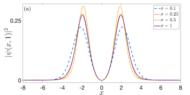
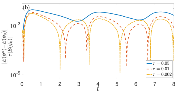
Figure 5.1. (a) density $|\psi(x,1)|^{2}$ with different $\sigma>0$ and (b) relative errors of the energy divided by $\tau$ up to $t=8$ with $\sigma=0.1$ for the Type I initial datum Equation 5.1 with $\beta=-10$.

In the following, we shall test the errors of the TSSP in $L^{2}$- and $H^{1}$-norms. We fix $d=1$, $T=1$ and $\beta=-1$. The NLSE Equation 1.1 is then solved by the TSSP method on the domain $\Omega$ with Type I and Type II initial setups for different $\sigma>0$. The ‘exact’ solution is obtained numerically by the Strang splitting sine pseudospectral method with a very fine mesh size $h_{e}=2^{-9}$ and a small time step size $\tau_{e}=10^{-6}$. In our numerical experiments below, when testing the temporal convergence, we always fix the mesh size $h=h_{e}$. To quantify the error, we introduce the following error functions:

$$e_{L^{2}}^{k}=\|\psi(\cdot,t_{k})-I_{N}\psi^{k}\|_{L^{2}},\quad e^{k}_{H^{1}}=\|\psi(\cdot,t_{k})-I_{N}\psi^{k}\|_{H^{1}},\quad 0\leq k\leq n:=T/\tau.$$

Figure 5.2 exhibits the temporal and spatial errors in $L^{2}$-norm of the TSSP Equation 2.13 for the NLSE Equation 1.1 with Type I initial datum and different $0<\sigma\leq 1/2$. Figure 5.2 (a) shows that the temporal convergence is first order in $L^{2}$-norm for all the four $\sigma$, and Figure 5.2 (b) shows the spatial convergence is almost third order in $L^{2}$-norm, which is also increasing with $\sigma$. These results are better than our error estimates in Theorem 2.5 and suggest that first order temporal convergence in $L^{2}$-norm may hold for any $\sigma>0$ and the spatial convergence may be of higher order. Similar results are also observed in our numerical experiments in 2D. However, we remark that it is impossible to obtain the optimal temporal convergence rates and the higher order spatial convergence rates by simply improving the local error estimates in Proposition 3.6, indicating that there must exist error cancellation between different steps, which require new techniques and in-depth analysis to handle. Also, we can observe similar temporal errors as in Figure 5.2 (a) for the Type II initial datum.

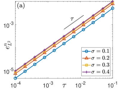
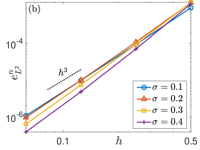
Figure 5.2. Temporal errors (a) and spatial errors (b) in $L^{2}$-norm for $\sigma=0.1,0.2,0.3,0.4$ with Type I initial datum Equation 5.1.

Figure 5.3 plots the temporal and spatial errors in $L^{2}$- and $H^{1}$-norm of the TSSP Equation 2.13 for the NLSE Equation 1.1 with Type II $H^{2}$ initial datum and fixed $\sigma=0.5$. Figure 5.3 (a) shows that the temporal convergence is first order in $L^{2}$-norm and half order in $H^{1}$-norm, and Figure 5.3 (b) shows the spatial convergence is second order in $L^{2}$-norm and first order in $H^{1}$-norm. These results correspond with our error estimates Equation 2.42 in Theorem 2.7 very well.

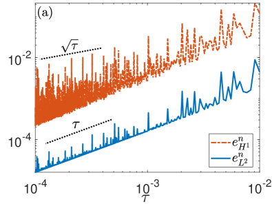
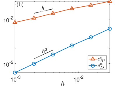
Figure 5.3. Temporal errors (a) and spatial errors (b) in $L^{2}$-norm and $H^{1}$-norm for $\sigma=0.5$ with Type II initial data Equation 5.2.

Figure 5.4 displays the temporal and spatial errors in $H^{1}$-norm of the TSSP Equation 2.13 for the NLSE Equation 1.1 with Type I smooth initial datum and different $0<\sigma<1$. Figure 5.4 (a) shows that the temporal convergence in $H^{1}$-norm increases from half order to first order as $\sigma$ increase from $0$ to $1/2$ and remains first order when $\sigma\geq 1/2$. Figure 5.4 (b) shows the spatial convergence is almost 2.5 order in $H^{1}$-norm and is increasing with $\sigma$. Similar to the observation of Figure 5.2, these results are better than our error estimates Equation 2.43 in Theorem 2.7 and suggest that first order temporal convergence in $H^{1}$-norm may hold for any $\sigma\geq 1/2$. We would like to comment that the order reduction in $H^{1}$-norm for $0<\sigma<1/2$ is indeed resulted from the semi-smoothness of the nonlinearity instead of the regularity of the exact solution. Actually, we numerically checked that with the Type I smooth initial datum, the exact solution is roughly in $H^{3.5+2\sigma}$.

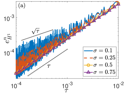
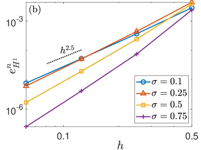
Figure 5.4. Temporal errors (a) and spatial errors (b) in $H^{1}$-norm for $\sigma=0.1,0.25,0.5,0.75$ with Type I initial datum Equation 5.1.

6. Conclusion

Error bounds of the Lie-Trotter splitting sine pseudospectral method for the nonlinear Schrödinger equation (NLSE) with semi-smooth nonlinearity $f(\rho)=\rho^{\sigma}(\sigma>0)$ were established. For $0<\sigma\leq\frac{1}{2}$, we prove error bounds at $O(\tau^{\frac{1}{2}+\sigma}+h^{1+2\sigma})$ in $L^{2}$-norm without any CFL-type time step size restrictions, where $\tau>0$ and $h>0$ are the time step size and mesh size respectively. For $\sigma\geq\frac{1}{2}$, error bounds at $O(\tau+h^{2})$ in $L^{2}$-norm and at $O(\tau^{\frac{1}{2}}+h)$ in $H^{1}$-norm are proved with mild time step size restrictions. In addition, when $\frac{1}{2}<\sigma<1$ and under the assumption of $H^{3}$-solution of the NLSE, we show an error bound at $O(\tau^{\sigma}+h^{2\sigma})$ in $H^{1}$-norm. Numerical results are reported to demonstrate our error estimates.

Appendix

Proof of Equation 4.49.

We shall present the proof in 1D, and one can easily generalize it to higher dimensions. By triangle inequality, recalling that $\phi_{j}=\phi(x_{j})$ for $j\in\mathcal{T}_{N}^{0}$,

$$\|{\delta_{x}^{+}}\phi\|_{l^{4}}^{4} =h\sum_{j=0}^{N-1}|{\delta_{x}^{+}}\phi_{j}|^{4}=h\sum_{j=0}^{N-1}|({\delta_{x}^{+}}\phi_{j})^{2}-({\delta_{x}^{+}}\phi_{0})^{2}+({\delta_{x}^{+}}\phi_{0})^{2}||{\delta_{x}^{+}}\phi_{j}|^{2}$$

$$\leq h\sum_{j=0}^{N-1}|({\delta_{x}^{+}}\phi_{j})^{2}-({\delta_{x}^{+}}\phi_{0})^{2}||{\delta_{x}^{+}}\phi_{j}|^{2}+h\sum_{j=0}^{N-1}|{\delta_{x}^{+}}\phi_{0}|^{2}|{\delta_{x}^{+}}\phi_{j}|^{2}$$

(6.1) $$=h\sum_{j=0}^{N-1}\left|\sum_{l=0}^{j-1}({\delta_{x}^{+}}\phi_{l+1})^{2}-({\delta_{x}^{+}}\phi_{l})^{2}\right||{\delta_{x}^{+}}\phi_{j}|^{2}+|{\delta_{x}^{+}}\phi_{0}|^{2}\|{\delta_{x}^{+}}\phi\|_{l^{2}}^{2}=:K_{1}+K_{2}.$$

We have separated the boundary terms $K_{2}$ from $K_{1}$. We start with the estimate of $K_{1}$, which is standard and can be obtained from the proof of the second inequality of (3.3) in [7]. We show it here for the convenience of the reader. Define the central difference operator ${\delta_{x}^{2}}$ as

(6.2) $${\delta_{x}^{2}}v_{j}:=\frac{v_{j+1}-2v_{j}+v_{j-1}}{h^{2}}=\frac{{\delta_{x}^{+}}v_{j}-{\delta_{x}^{+}}v_{j-1}}{h},\quad 1\leq j\leq N-1,\quad v\in Y_{N}.$$

For $K_{1}$ defined in Proof of Equation 4.49., using triangle inequality and Cauchy inequality, we get

$$K_{1} \leq h\sum_{j=0}^{N-1}\sum_{l=0}^{N-2}|{\delta_{x}^{+}}\phi_{l+1}+{\delta_{x}^{+}}\phi_{l}||{\delta_{x}^{+}}\phi_{l+1}-{\delta_{x}^{+}}\phi_{l}||{\delta_{x}^{+}}\phi_{j}|^{2}$$

$$\leq h\sum_{j=0}^{N-1}|{\delta_{x}^{+}}\phi_{j}|^{2}\sqrt{\sum_{l=0}^{N-2}|{\delta_{x}^{+}}\phi_{l+1}+{\delta_{x}^{+}}\phi_{l}|^{2}}\sqrt{\sum_{l=0}^{N-2}|{\delta_{x}^{+}}\phi_{l+1}-{\delta_{x}^{+}}\phi_{l}|^{2}}$$

(6.3) $$\lesssim\|{\delta_{x}^{+}}\phi\|_{l^{2}}^{2}\sqrt{h\sum_{l=0}^{N-1}|{\delta_{x}^{+}}\phi_{l}|^{2}}\sqrt{h\sum_{l=1}^{N-1}|{\delta_{x}^{2}}\phi_{l}|^{2}}=\|{\delta_{x}^{+}}\phi\|_{l^{2}}^{3}\sqrt{h\sum_{l=1}^{N-1}|{\delta_{x}^{2}}\phi_{l}|^{2}}.$$

Since $\phi\in X_{N}$, we have

(6.4) $$\phi_{j}=\phi(x_{j})=\sum_{l=1}^{N-1}\widehat{\phi}_{l}\sin(\mu_{l}(x_{j}-a))=\sum_{l=1}^{N-1}\widehat{\phi}_{l}\sin(\mu_{l}jh),\quad 0\leq j\leq N,$$

which implies, by recalling Equation 6.2,

(6.5) $${\delta_{x}^{2}}\phi_{j}=\frac{\phi_{j+1}-2\phi_{j}+\phi_{j-1}}{h^{2}}=-\sum_{l=1}^{N-1}\mu_{l}^{2}\widehat{\phi}_{l}\left|\operatorname{sinc}(\mu_{l}h/2)\right|^{2}\sin(\mu_{l}jh),$$

where $\operatorname{sinc}(x)=\sin(x)/x$ for $x\in\mathbb{R}$ with $\operatorname{sinc}(0)=1$. By Parseval’s identity, noting Equation 6.5 and $|\operatorname{sinc}(x)|\leq 1$ for $x\in\mathbb{R}$, we get (similar to the proof of Equation 4.36)

(6.6) $$h\sum_{j=1}^{N-1}|{\delta_{x}^{2}}\phi_{j}|^{2}=\frac{Nh}{2}\sum_{l=1}^{N-1}\mu_{l}^{4}\left|\widehat{\phi}_{l}\right|^{2}\left|\operatorname{sinc}(\mu_{l}h/2)\right|^{4}\leq\frac{Nh}{2}\sum_{l=1}^{N-1}\mu_{l}^{4}\left|\widehat{\phi}_{l}\right|^{2}\leq\|\phi\|_{H^{2}}^{2}.$$

Plugging Equation 6.6 into Proof of Equation 4.49. and using Equation 4.36, we have

(6.7) $$K_{1}\lesssim\|\phi\|_{H^{2}}\|\phi\|_{H^{1}}^{3}\leq\|\phi\|_{H^{2}}^{4}.$$

For $K_{2}$ in Proof of Equation 4.49., recalling Equation 6.4 and $|\operatorname{sinc}(x)|\leq 1$ for $x\in\mathbb{R}$, and noting that $\sum_{l=1}^{\infty}|\mu_{l}|^{-2}<\infty$, we have, by Cauchy inequality,

$$|{\delta_{x}^{+}}\phi_{0}|=\left|\frac{\phi_{1}}{h}\right|=\left|\sum_{l=1}^{N-1}\mu_{l}\widehat{\phi}_{l}\operatorname{sinc}(\mu_{l}h)\right|\leq\sqrt{\sum_{l=1}^{N-1}|\mu_{l}|^{4}|\widehat{\phi}_{l}|^{2}}\sqrt{\sum_{l=1}^{N-1}|\mu_{l}|^{-2}}\lesssim\|\phi\|_{H^{2}},$$

which implies, by using Equation 4.36 again,

(6.8) $$K_{2}=|{\delta_{x}^{+}}\phi_{0}|^{2}\|{\delta_{x}^{+}}\phi\|_{l^{2}}^{2}\lesssim\|\phi\|_{H^{2}}^{2}\|\nabla\phi\|_{H^{1}}^{2}\leq\|\phi\|_{H^{2}}^{4}.$$

Plugging Equations 6.7 and 6.8 into Proof of Equation 4.49. yields the desired result. ∎

References

- [1] G. D. Akrivis, Finite difference discretization of the cubic Schrödinger equation, IMA J. Numer. Anal. 13 (1993), no. 1, 115–124. MR 1199033
- [2] G. D. Akrivis, V. A. Dougalis, and O. A. Karakashian, On fully discrete Galerkin methods of second-order temporal accuracy for the nonlinear Schrödinger equation, Numer. Math. 59 (1991), no. 1, 31–53. MR 1103752
- [3] X. Antoine, W. Bao and C. Besse, Computational methods for the dynamics of the nonlinear Schrödinger/Gross-Pitaevskii equations, Comput. Phys. Commun. 184 (2013), 2621–2633.
- [4] G. E. Astrakharchik and B. A. Malomed, Dynamics of one-dimensional quantum droplets, Phys. Rev. A 98 (2018), 013631.
- [5] W. Bao and Y. Cai, Uniform error estimates of finite difference methods for the nonlinear Schrödinger equation with wave operator, SIAM J. Numer. Anal. 50 (2012), no. 2, 492–521. MR 2914273
- [6] W. Bao and Y. Cai, Mathematical theory and numerical methods for Bose-Einstein condensation, Kinet. Relat. Models 6 (2013), no. 1, 1–135. MR 3005624
- [7] W. Bao and Y. Cai, Optimal error estimates of finite difference methods for the Gross-Pitaevskii equation with angular momentum rotation, Math. Comp. 82 (2013), no. 281, 99–128. MR 2983017
- [8] W. Bao and Y. Cai, Uniform and optimal error estimates of an exponential wave integrator sine pseudospectral method for the nonlinear Schrödinger equation with wave operator, SIAM J. Numer. Anal. 52 (2014), no. 3, 1103–1127. MR 3199421
- [9] W. Bao, R. Carles, C. Su, and Q. Tang, Error estimates of a regularized finite difference method for the logarithmic Schrödinger equation, SIAM J. Numer. Anal. 57 (2019), no. 2, 657–680. MR 3928348
- [10] W. Bao, R. Carles, C. Su, and Q. Tang, Regularized numerical methods for the logarithmic Schrödinger equation, Numer. Math. 143 (2019), no. 2, 461–487. MR 4009693
- [11] W. Bao, R. Carles, C. Su, and Q. Tang, Error estimates of local energy regularization for the logarithmic Schrödinger equation, Math. Models Methods Appl. Sci. 32 (2022), no. 1, 101–136. MR 4379522
- [12] W. Bao, Y. Feng, and Y. Ma, Regularized numerical methods for the nonlinear Schrödinger equation with singular nonlinearity, East Asian J. Appl. Math., 13(3) (2023), 646-670. MR 4600450
- [13] W. Bao, D. Jaksch, and P. A. Markowich, Numerical solution of the Gross-Pitaevskii equation for Bose-Einstein condensation, J. Comput. Phys. 187 (2003), no. 1, 318–342. MR 1977789
- [14] W. Bao, N. J. Mauser, and H. P. Stimming, Effective one particle quantum dynamics of electrons: a numerical study of the Schrödinger-Poisson- model, Commun. Math. Sci. 1 (2003), no. 4, 809–828. MR 2041458
- [15] C. Besse, B. Bidégaray, and S. Descombes, Order estimates in time of splitting methods for the nonlinear Schrödinger equation, SIAM J. Numer. Anal. 40 (2002), no. 1, 26–40. MR 1921908
- [16] O. Bokanowski and N. J. Mauser, Local approximation for the Hartree-Fock exchange potential: a deformation approach, Math. Models Methods Appl. Sci. 9 (1999), no. 6, 941–961. MR 1702877
- [17] C. R. Cabrera, L. Tanzi, J. Sanz, B. Naylor, P. Thomas, P. Cheiney, and L. Tarruell, Quantum liquid droplets in a mixture of Bose-Einstein condensates, Science 359 (2018), no. 6373, 301–304.
- [18] Y. Cai and H. Wang,, Analysis and computation for ground state solutions of Bose-Fermi mixtures at zero temperature, SIAM J. Appl. Math. 73 (2013), 757–779.
- [19] T. Cazenave, Semilinear Schrödinger equations, Courant Lecture Notes in Mathematics, vol. 10, New York University, Courant Institute of Mathematical Sciences, New York; American Mathematical Society, Providence, RI, 2003. MR 2002047
- [20] E. Celledoni, D. Cohen, and B. Owren, Symmetric exponential integrators with an application to the cubic Schrödinger equation, Found. Comput. Math. 8 (2008), no. 3, 303–317. MR 2413146
- [21] W. Choi and Y. Koh, On the splitting method for the nonlinear Schrödinger equation with initial data in , Discrete Contin. Dyn. Syst. 41 (2021), no. 8, 3837–3867. MR 4251835
- [22] J. Eilinghoff, R. Schnaubelt, and K. Schratz, Fractional error estimates of splitting schemes for the nonlinear Schrödinger equation, J. Math. Anal. Appl. 442 (2016), no. 2, 740–760. MR 3504024
- [23] L. Erdős, B. Schlein, and H.-T. Yau, Derivation of the cubic non-linear Schrödinger equation from quantum dynamics of many-body systems, Invent. Math. 167 (2007), no. 3, 515–614. MR 2276262
- [24] Z. Hadzibabic, C. A. Stan, K. Dieckmann, S. Gupta, M. W. Zwierlein, A. Gorlitz, and W. Ketterle, Two-species mixture of quantum degenerate Bose and Fermi gases, Phys. Rev. Lett. 88 (2002), 160401.
- [25] P. Henning and D. Peterseim, Crank-Nicolson Galerkin approximations to nonlinear Schrödinger equations with rough potentials, Math. Models Methods Appl. Sci., 27 (2017), pp. 2147–2184. MR 3691815
- [26] M. Hochbruck and A. Ostermann, Exponential integrators, Acta Numer. 19 (2010), 209–286. MR 2652783
- [27] Y. Hu, Y. Fei, X.-L. Chen, and Y. Zhang, Collisional dynamics of symmetric two-dimensional quantum droplets, Frontiers of Physics 17 (2022), no. 6, 61505.
- [28] L. I. Ignat, A splitting method for the nonlinear Schrödinger equation, J. Differential Equations 250 (2011), no. 7, 3022–3046. MR 2771254
- [29] H. Kadau, M. Schmitt, M. Wenzel, C. Wink, T. Maier, I. Ferrier-Barbut, and T. Pfau, Observing the rosensweig instability of a quantum ferrofluid, Nature 530 (2016), no. 7589, 194–197.
- [30] T. Kato, On nonlinear Schrödinger equations, Ann. Inst. H. Poincaré Phys. Théor., 46 (1987), pp. 113–129.
- [31] M. Knöller, A. Ostermann, and K. Schratz, A Fourier integrator for the cubic nonlinear Schrödinger equation with rough initial data, SIAM J. Numer. Anal. 57 (2019), no. 4, 1967–1986. MR 3992056
- [32] T. D. Lee, K. Huang, and C. N. Yang, Eigenvalues and eigenfunctions of a Bose system of hard spheres and its low-temperature properties, Phys. Rev. 106 (1957), 1135–1145.
- [33] C. Lubich, On splitting methods for Schrödinger-Poisson and cubic nonlinear Schrödinger equations, Math. Comp. 77 (2008), no. 264, 2141–2153. MR 2429878
- [34] A. Ostermann, F. Rousset, and K. Schratz, Error estimates at low regularity of splitting schemes for NLS, Math. Comp. 91 (2021), no. 333, 169–182. MR 4350536
- [35] A. Ostermann, F. Rousset, and K. Schratz, Error estimates of a Fourier integrator for the cubic Schrödinger equation at low regularity, Found. Comput. Math. 21 (2021), no. 3, 725–765. MR 4269650
- [36] A. Ostermann and K. Schratz, Low regularity exponential-type integrators for semilinear Schrödinger equations, Found. Comput. Math. 18 (2018), no. 3, 731–755. MR 3807360
- [37] A. Ostermann, Y. Wu, and F. Yao, A second-order low-regularity integrator for the nonlinear Schrödinger equation, Adv. Contin. Discrete Models (2022), Paper No. 23, 14. MR 4395149
- [38] A. Ostermann and F. Yao, A fully discrete low-regularity integrator for the nonlinear Schrödinger equation, J. Sci. Comput. 91 (2022), no. 1, Paper No. 9, 14. MR 4385374
- [39] D. S. Petrov and G. E. Astrakharchik, Ultradilute low-dimensional liquids, Phys. Rev. Lett. 117 (2016), 100401.
- [40] A. Porretta, A note on the Sobolev and Gagliardo-Nirenberg inequality when , Adv. Nonlinear Stud. 20 (2020), no. 2, 361–371. MR 4095474
- [41] F. Rousset and K. Schratz, A general framework of low regularity integrators, SIAM J. Numer. Anal. 59 (2021), no. 3, 1735–1768. MR 4275500
- [42] J. M. Sanz-Serna, Methods for the numerical solution of the nonlinear Schrödinger equation, Math. Comp. 43 (1984), no. 167, 21–27. MR 744922
- [43] J. Shen, T. Tang, and L.-L. Wang, Spectral Methods: Algorithms, Analysis and Applications, Springer Series in Computational Mathematics, vol. 41, Springer, Heidelberg, 2011. MR 2867779
- [44] C. Sulem and P.-L. Sulem, The nonlinear Schrödinger equation: Self-focusing and wave collapse, Applied Mathematical Sciences, Springer New York, NY, 1999.
- [45] Y. Tourigny, Optimal estimates for two time-discrete Galerkin approximations of a nonlinear Schrödinger equation, IMA J. Numer. Anal. 11 (1991), no. 4, 509–523. MR 1135202
- [46] J. Wang, A new error analysis of Crank-Nicolson Galerkin FEMs for a generalized nonlinear Schrödinger equation, J. Sci. Comput. 60 (2014), no. 2, 390–407. MR 3225788