Why Batch Normalization Damage Federated Learning
on Non-IID Data?

Abstract

As a promising distributed learning paradigm, federated learning (FL) involves training deep neural network (DNN) models at the network edge while protecting the privacy of the edge clients. To train a large-scale DNN model, batch normalization (BN) has been regarded as a simple and effective means to accelerate the training and improve the generalization capability. However, recent findings indicate that BN can significantly impair the performance of FL in the presence of non-i.i.d. data. While several FL algorithms have been proposed to address this issue, their performance still falls significantly when compared to the centralized scheme. Furthermore, none of them have provided a theoretical explanation of how the BN damages the FL convergence. In this paper, we present the first convergence analysis to show that under the non-i.i.d. data, the mismatch between the local and global statistical parameters in BN causes the gradient deviation between the local and global models, which, as a result, slows down and biases the FL convergence. In view of this, we develop a new FL algorithm that is tailored to BN, called FedTAN, which is capable of achieving robust FL performance under a variety of data distributions via iterative layer-wise parameter aggregation. Comprehensive experimental results demonstrate the superiority of the proposed FedTAN over existing baselines for training BN-based DNN models.

1 Introduction

The traditional centralized learning systems, as illustrated in Fig. 1(a), involves collecting data samples from edge clients and generating a global dataset at the server. This creates a huge transmission cost as well as privacy concerns. In order to overcome these issues, federated learning (FL) in Fig. 1(b) has been proposed as a technique for training deep neural networks (DNNs) over distributed edge clients without accessing their raw data [1, 2, 3]. However, due to heterogeneous local datasets in practice, FL is facing the inter-client variance problem, and various FL algorithms have been proposed to address this issue. For example, FedProx in [4] introduces a regularization term in local objective functions to control model divergence. SCAFFOLD in [5] corrects drift in local models using control variates. FedALRC in [6] incorporates a regularization scheme to constrain the local Rademacher complexity, enhancing the generalization ability of FL. Moreover, the work in [7] proposes sparse ternary compression, which relies on frequent communication of weight updates between clients to mitigate divergence among local models. However, most of these studies primarily concentrated on training small to moderate-sized DNN models. Despite the challenge posed by the extensive computations and substantial data access required for training large-scale DNN models, the rapid advancements in computing power in recent years have sparked a growing interest in utilizing FL networks for training such models [2, 8, 9, 10, 11]. In order to accelerate the training process and improve the generalization capability of large-scale DNN models, data normalization techniques such as batch normalization (BN) and group normalization (GN) are used [12, 13]. It is interesting to note that recent studies have suggested that BN may negatively impact FL [2, 10, 11]. For instance, the work in [2] found that when clients have i.i.d. data, the ResNet-20 model trained with BN [14] can achieve a testing accuracy of 85%, but when the local data are non-i.i.d., the accuracy drops dramatically to 60%. This is because that with BN, the parameters of every DNN layer are determined by the statistics associated with its local input. Thus, when the local datasets at the clients are non-i.i.d., there is a mismatch between the local data statistics and the global data statistics, which makes the gradients computed by the local datasets greatly differ from the global gradient computed by the global dataset. In view of the fact that BN has demonstrated its success in the DNN training and has become a fundamental component of many state-of-the-art DNN models [15], it is crucial to fix the issue and develop efficient FL algorithms with BN.

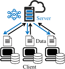
(a) Centralized Learning

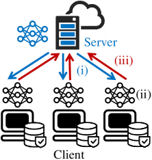
(b) Federated Learning

Figure 1: Centralized learning v.s. Federated Learning.

1.1 Related Works

In recent years, several attempts have been made toward this direction. Firstly, some works replaced BN with alternative normalization mechanisms that do not rely on batch samples. For example, to recover the accuracy loss caused by BN in the non-i.i.d. setting, the works [16] and [17] replace BN with Group Normalization (GN) and Layer Normalization (LN), respectively. However, these alternative normalization mechanisms have some disadvantages. Specifically, GN is an instance-based method of normalization, which is highly sensitive to the noise in data samples, while LN assumes that the inputs to all neurons within the same DNN layer contribute equally to the final inference [16, 17]. In this regard, BN is likely to outperform GN and LN for some applications in terms of a faster convergence rate and higher testing accuracy.

Secondly, some studies adopted the local BN technique to reduce the gradient drift of local models under non-i.i.d. data. For example, FedBN in [15] trains all BN parameters (including batch mean, batch variance, scale parameter, and shift parameter) locally in clients based on only the local datasets, while SiloBN [18] updates only the batch mean and batch variance locally in clients but sharing other BN parameters including the scale and shift parameters with the server for global aggregation. Different from [18], the work in [19] suggests that updating both scale and shift parameters locally while aggregating batch mean and batch variance globally would achieve faster FL convergence. However, all of the above methods would still perform unsatisfyingly in a general non-i.i.d. scenario where the clients have different label distributions (e.g., the data of each client contains only a subset of labels and they are different to each other). Therefore, to guarantee FL convergence under such general non-i.i.d. data cases, it is insufficient to aggregate only part of the DNN model parameters at the server while keeping some BN parameters updated in clients.

In view of this, several recent FL works have considered aggregating all DNN model parameters at the server while modifying the mode of updating BN parameters. Some studies considered modifying the aggregation scheme at the server side. For instance, FedBS in [20] introduces a heuristic weighted aggregation scheme on local model parameters and BN parameters, by giving a greater weight to clients with a higher local loss function value. FedDNA in [21] adopts an importance weighting method to aggregate local batch means and batch variances, but requires the server to train an additional adversarial model to calculate the weighting coefficients. Some works considered modifying the local model updating steps at the client side. As an example, the work in [22] utilizes a fine-tuning technique to train BN parameters in local models, where if the validation accuracy of a local model does not improve, only its BN parameters are updated and the remaining network coefficients are frozen. The above methods maintain tracking of the moving average of batch mean and batch variance throughout the entire training process and also utilizes it for model inference as a common technique in BN. Unlike the previous approaches, HeteroFL in [23] proposed a static BN approach that does not track the moving average but instead makes use of the instantaneous output statistics of DNN layers in model inference. Even so, the performance of the above works still drop significantly under the general non-i.i.d. data case. Besides, none of them have examined the theoretical impact of BN on the FL convergence speed.

Furthermore, the FL works above only observe that under the non-i.i.d. data, the mismatch between the local and global statistical parameters (including batch mean and batch variance) obtained in the forward propagation procedure would adversely affect the FL performance. However, they overlooked that the mismatch between the local and global gradients with respect to (w.r.t.) statistical parameters computed during the backward propagation procedure also harms FL convergence.

1.2 Contributions

This paper investigates why BN damages FL on the non-i.i.d. data. We highlight that there are two types of mismatches that jointly influence the convergence of FL with BN: one is the mismatch between the local and global statistical parameters, and the other is that between the related local and global gradients w.r.t. statistical parameters. Specifically, in the previous research aimed at improving the FL performance with BN, only the statistical parameters obtained in the forward propagation are noted, whereas the gradients w.r.t. statistical parameters computed in the backward propagation are ignored. Unfortunately, the gradients w.r.t. statistical parameters are intermediate variables in calculating the gradients w.r.t. the DNN model parameters in the training process, and thereby have a significant impact on the convergence of FL. This is the fundamental reason why the previous methods still suffer performance loss.

In view of this, we present the first theoretical analysis of how the above two types of mismatches caused by BN and non-i.i.d data degrade the convergence of FedAvg [24]. To overcome this effect, we further propose a new FL algorithm, named FedTAN (federated learning algorithm tailored for batch normalization), which eliminates the two types of mismatches above by layer-wise statistical parameter aggregation and can achieve robust FL performance under different data distributions. In particular, our main contributions include:

1. Convergence analysis of FL with BN: We consider the general non-convex FL problems. To the best of our knowledge, we are the first to analyze theoretically how BN affects the convergence rate of FedAvg. The derived theoretical results indicate that the gradient deviation would occur in local models if the local statistical parameters in BN and the related gradients are inconsistent with the global ones obtained by the global dataset. As a consequence, the resulting gradient deviation not only slows down, but also biases the convergence of FL.

2. Relation analysis between local and global statistical parameters as well as their gradients: The formal mathematical expressions of both the i.i.d. and the non-i.i.d. data cases are defined. Based on this, we conclude that the i.i.d. data leads to the same local and global statistical parameters as well as their gradients, whereas the non-i.i.d. data produces the mismatches. Also, we find that merely eliminating the mismatch between local and global statistical parameters, without ensuring consistency between local and global gradients w.r.t. statistical parameters, cannot guarantee FL convergence.

3. FedTAN: The above observations suggest that if all clients in FL have the same statistical parameters and related gradients as the global ones, then undesirable slowdown caused by gradient deviation under BN can be eliminated. Inspired by this, we develop a new FL algorithm, FedTAN, which leverages layer-wise aggregation to match not only the local and global statistical parameters during forward propagation but also their associated gradients during backward propagation.

4. Experiments: FedTAN is applied to classify color images in the CIFAR-10 dataset. Experimental results indicate that FedTAN has promising performance and outperforms benchmark schemes. In particular, we show that even though FedTAN requires extra message exchanges between the clients and the server, it is still capable of achieving a satisfying training performance and faster convergence rate under different data distributions.

Synopsis: Section 2 introduces the FL algorithm on a DNN model with BN layers. Section 3 analyzes the convergence of FL with BN, while Section 4 examines the relations between the local and global statistical parameters as well as their gradients, under different data distributions. Based on the theoretical results, Section 5 develops an FL algorithm tailored for BN. Experimental results are presented in Section 6, and finally, Section 7 concludes this paper.

2 Federated Learning with Batch Normalization

2.1 Batch Normalization

As shown in Fig. 2, we follow the similar architecture as the plain layer-by-layer network in [14] and consider a DNN with $L$ BN layers. Each feature extraction layer except the input layer (i.e., the 0-th layer) is preceded by a BN layer, and each feature extraction layer can be composed of a convolution layer, a fully-connected layer, a pooling layer, a flatten layer, or an activation layer, etc.

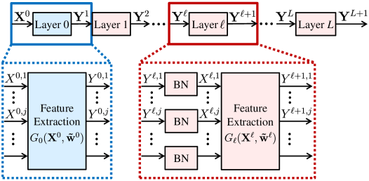
Figure 2: An example of DNN model with BN layers. Each feature extraction layer can be comprised of convolution layer, fully-connected layer, pooling layer, flatten layer, activation layer, etc.

Let $\mathbf{Y}^{\ell}$ represent the input to the $\ell$-th BN layer, for $\ell=1,\ldots,L$. Then, each $j$-th element of $\mathbf{Y}^{\ell}$ is normalized as

$$X^{\ell,j}=\gamma^{\ell,j}\underbrace{\frac{Y^{\ell,j}-\mu^{\ell,j}}{\sqrt{(\sigma^{\ell,j})^{2}+\epsilon}}}_{\triangleq{\hat{Y}}^{\ell,j}}+\beta^{\ell,j},$$ (1)

where $\gamma^{\ell,j}$ is a scale parameter, $\beta^{\ell,j}$ is a shift parameter, and $\epsilon$ is a small positive value. Here, batch mean $\mu^{\ell,j}$ and batch variance $(\sigma^{\ell,j})^{2}$ are obtained by

$$\mu^{\ell,j}=\mathbb{E}_{\mathcal{D}}[Y^{\ell,j}],$$ (2a)

$$(\sigma^{\ell,j})^{2}=\mathbb{E}_{\mathcal{D}}[(Y^{\ell,j}-\mu^{\ell,j})^{2}],$$ (2b)

where $\mathbb{E}_{\mathcal{D}}[\cdot]$ is the expectation over the data samples $\mathcal{D}$. After that, the output of the BN layer, $\mathbf{X}^{\ell}$, is fed into its subsequent feature extraction layer with the computation function as

$$\mathbf{Y}^{\ell+1}=G_{\ell}(\mathbf{X}^{\ell},\mathbf{\tilde{w}}^{\ell}),\,\ell=0,\ldots,L,$$ (3)

where $\mathbf{\tilde{w}}^{\ell}$ is the network coefficients and $\mathbf{Y}^{\ell+1}$ is the output.

For a DNN with BN, the model parameters include both the gradient parameters (denoted by $\mathbf{w}$) which are commonly contained in all layers and updated by model gradients, and the statistical parameters (denoted by $\mathcal{S}$) which are solely contained in BN layers and updated by the statistics of intermediate outputs in DNN [21]. The gradient parameters $\mathbf{w}$ consist of both the network coefficients $\{\mathbf{\tilde{w}}^{\ell}\}$ as well as the scale parameters $\bm{\gamma}^{\ell}(=\{\gamma^{\ell,j}\})$ and shift parameters $\bm{\beta}^{\ell}(=\{\beta^{\ell,j}\})$, while the statistical parameters are batch mean $\bm{\mu}^{\ell}(=\{\mu^{\ell,j}\})$ and batch variance $(\bm{\sigma}^{\ell})^{2}(=\{(\sigma^{\ell,j})^{2}\})$. Thus, the model parameters in a DNN are $\mathbf{W}=\{\mathbf{w},\mathcal{S}\}$. It is important to note that $\mathbf{w}$ and $\mathcal{S}$ are interdependent.

In order to train a DNN to minimize a particular cost function $F({\mathbf{W}})$, the gradient of $F$ w.r.t. the gradient parameters $\mathbf{w}$, $\nabla_{\mathbf{w}}F$, must be computed. However, when using BN, $\nabla_{\mathbf{w}}F$ is a function not only of the gradient parameters $\mathbf{w}$, but also of the statistical parameters $\mathcal{S}$ and their gradients $\Delta\mathcal{S}\triangleq\{\nabla_{\bm{\mu}^{\ell}}F,\nabla_{(\bm{\sigma}^{\ell})^{2}}F\}$. Specifically, $\mathcal{S}$ and $\Delta\mathcal{S}$ are used in the forward and backward propagations, respectively, to calculate $\nabla_{\mathbf{w}}F$ [25]. Thus, we write $\nabla_{\mathbf{w}}F$ explicitly as $\nabla_{\mathbf{w}}F(\mathbf{w};\mathcal{S},\Delta\mathcal{S})$.

2.2 Federated Learning Algorithm

As shown in Fig. 1(b), the FL scheme involves a server coordinating $N$ clients to solve the following learning problem

$$\min\limits_{{\mathbf{W}}}\;F({\mathbf{W}})=\sum_{i=1}^{N}p_{i}F_{i}({\mathbf{W}}),$$ (4)

where $p_{i}={|\mathcal{D}_{i}|}/{|\mathcal{D}|}$, $\mathcal{D}_{i}$ is the local dataset in client $i$, $\mathcal{D}=\bigcup_{i=1}^{N}\mathcal{D}_{i}$ is the global dataset, $F({\mathbf{W}})=\mathbb{E}_{\mathcal{D}}[\mathcal{L}({\mathbf{W}};\mathcal{D})]$ is the global cost function on $\mathcal{D}$ and $F_{i}({\mathbf{W}})=\mathbb{E}_{\mathcal{D}_{i}}[\mathcal{L}({\mathbf{W}};\mathcal{D}_{i})]$ is the local one on $\mathcal{D}_{i}$ in which $\mathcal{L}$ is the loss function of data samples. This paper considers the celebrated FedAvg algorithm [24], which executes the following three steps every ${r}$-th iteration:

1. Initialization: All clients receive the global model $\{{\bar{\mathbf{w}}}_{r-1},{\bar{\mathcal{S}}}_{r-1}\}$ in the last iteration from the server.

2. Local model updating: Each client $i\in[N]\triangleq\{1,\ldots,N\}$ updates its local gradient parameters through $E$ successive steps of local gradient descent. Specifically, initialize the local model by (5a) and perform (5b) for $t\in[E]$.

   $$\{\mathbf{w}^{r,0}_{i},{\bar{\mathcal{S}}}^{r,0}_{\mathcal{D}_{i}}\}=\{{\bar{\mathbf{w}}}_{r-1},{\bar{\mathcal{S}}}_{r-1}\},$$ (5a)

   $$\mathbf{w}^{r,t}_{i}={\mathbf{w}}^{r,t-1}_{i}-\gamma\nabla_{\mathbf{w}}F_{i}({\mathbf{w}}^{r,t-1}_{i};{\mathcal{S}}^{r,t}_{\mathcal{D}_{i}},\Delta{\mathcal{S}}^{r,t}_{\mathcal{D}_{i}}),$$ (5b)

   where $\gamma>0$ is the learning rate, $E$ is the number of local updating steps, and ${\mathcal{S}}^{r,t}_{\mathcal{D}_{i}}$ is the statistical parameters computed via (2) with the local model ${\mathbf{w}}^{r,t-1}_{i}$ and the local dataset $\mathcal{D}_{i}$. During this time, each client updates local statistical parameters for model inference by moving average as [22]

   $${\bar{\mathcal{S}}}^{r,t}_{\mathcal{D}_{i}}=(1-\rho){\bar{\mathcal{S}}}^{r,t-1}_{\mathcal{D}_{i}}+\rho{\mathcal{S}}^{r,t}_{\mathcal{D}_{i}},\,t\in[E],$$ (6)

   where $\rho$ is the momentum of moving average.

3. Aggregation: The local model $\{\mathbf{w}_{i}^{r,E},{\bar{\mathcal{S}}}^{r,E}_{\mathcal{D}_{i}}\}$ in each client $i\in[N]$ is uploaded to the server for aggregating a new global model by

   $$\{{\bar{\mathbf{w}}}_{r},{\bar{\mathcal{S}}}_{r}\}=\sum_{i=1}^{N}p_{i}\{\mathbf{w}^{r,E}_{i},{\bar{\mathcal{S}}}^{r,E}_{\mathcal{D}_{i}}\}.$$ (7)

It is found that FL with BN performs much worse under the non-i.i.d. local datasets, even when $E=1$ [2, 10, 11]. As an example, Fig. 3 compares the testing accuracy of different FL schemes on training ResNet-20 [14] under different data distributions, where $E=1$ and detailed settings are presented in Section 6. Firstly, according to Fig. 3(a), FedAvg is unable to train such a large model effectively without BN, whereas BN greatly improves performance when applied. Secondly, based on the theory on FL convergence in the current research [26, 27, 28], FedAvg with $E=1$ should perform similarly to the centralized learning with a larger batch size. However, Fig. 3(b) shows that FedAvg+BN suffers serious degradation when the data becomes non-i.i.d. Additionally, the performance of advanced FL algorithms like FedProx [4] and SCAFFOLD [5] is also poor. As a result, it is necessary to understand how the BN damages FL performance under non-i.i.d data and propose a remedy.

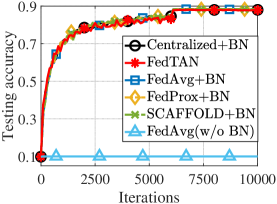
(a) The i.i.d. data case.

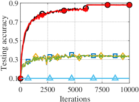
(b) The non-i.i.d. data case.

Figure 3: FL performance with BN and $E=1$. ResNet-20 is trained by CIFAR-10 dataset.

3 How BN damages FL?

3.1 Gradient Deviation under BN

The reason why BN damages FL is that under the distributed setting, the local statistical parameters and their gradients differ from the global ones, resulting in an inconsistency between the global gradient and the average of local gradients computed by clients. On general non-convex optimization problems, it appears from (4) and the analyses in [29, 28, 4, 5] that, the FL convergence is particularly sensitive to the following condition

$$\nabla_{\mathbf{w}}F({\mathbf{W}})=\sum_{i=1}^{N}p_{i}\nabla_{\mathbf{w}}F_{i}({\mathbf{W}}).$$ (8)

However, when BN is used, $\mathbf{W}$ includes both gradient parameters and statistical parameters. Consequently, (8) holds only if the left-hand side (LHS) and the right-hand side (RHS) of (8) are determined by the same $\mathcal{S}$ and $\Delta\mathcal{S}$, i.e.,

$$\nabla_{\mathbf{w}}F({\mathbf{w}};\mathcal{S}_{\mathcal{D}},\Delta\mathcal{S}_{\mathcal{D}})=\sum_{i=1}^{N}p_{i}\nabla_{\mathbf{w}}F_{i}({\mathbf{w}};\mathcal{S}_{\mathcal{D}},\Delta\mathcal{S}_{\mathcal{D}}),$$ (9)

where $\mathcal{D}=\bigcup_{i=1}^{N}\mathcal{D}_{i}$ refers to the global dataset.

Unfortunately, in the FL setting, each client $i$ can only access its local dataset $\mathcal{D}_{i}$ and, as a result, can only compute $\nabla_{\mathbf{w}}F_{i}({\mathbf{w}};\mathcal{S}_{\mathcal{D}_{i}},\Delta\mathcal{S}_{\mathcal{D}_{i}})$.

Observation 1

In the non-i.i.d. data case, the local dataset $\mathcal{D}_{i}$ and global dataset $\mathcal{D}$ generally cause $\mathcal{S}_{\mathcal{D}_{i}}\neq\mathcal{S}_{\mathcal{D}}$ and $\Delta\mathcal{S}_{\mathcal{D}_{i}}\neq\Delta\mathcal{S}_{\mathcal{D}}$. As a result, we have

$$\nabla_{\mathbf{w}}F_{i}({\mathbf{w}};\mathcal{S}_{\mathcal{D}_{i}},\Delta\mathcal{S}_{\mathcal{D}_{i}})\neq\nabla_{\mathbf{w}}F_{i}({\mathbf{w}};\mathcal{S}_{\mathcal{D}},\Delta\mathcal{S}_{\mathcal{D}}).$$ (10)

A formal discussion about this observation will be provided in Section 4.2. Then, substituting (10) into (9), we have

$$\nabla_{\mathbf{w}}F({\mathbf{w}};\mathcal{S}_{\mathcal{D}},\Delta\mathcal{S}_{\mathcal{D}})\neq\sum_{i=1}^{N}p_{i}\nabla_{\mathbf{w}}F_{i}({\mathbf{w}};\mathcal{S}_{\mathcal{D}_{i}},\Delta\mathcal{S}_{\mathcal{D}_{i}}),$$ (11)

which contradicts the default assumption in (8). Hence, to characterize the gradient deviation resulting from both the mismatched statistical parameters and the mismatched gradients w.r.t. statistical parameters, we introduce Assumption 1.

Assumption 1

The gradient deviation under BN satisfies $\|\nabla_{\mathbf{w}}F_{i}({\bar{\mathbf{w}}}_{r-1};\mathcal{S}_{\mathcal{D}_{i}}^{r,1},\Delta\mathcal{S}_{\mathcal{D}_{i}}^{r,1})-\nabla_{\mathbf{w}}F_{i}({\bar{\mathbf{w}}}_{r-1};\mathcal{S}_{\mathcal{D}}^{r,1},\Delta\mathcal{S}_{\mathcal{D}}^{r,1})\|^{2}$ $\leq B_{i}^{2}$, $\forall i\in[N]$.

It is important to note that Assumption 1 considers the discrepancy between $\{\mathcal{S}_{\mathcal{D}_{i}}^{r,1},\Delta\mathcal{S}_{\mathcal{D}_{i}}^{r,1}\}$ and $\{\mathcal{S}_{\mathcal{D}}^{r,1},\Delta\mathcal{S}_{\mathcal{D}}^{r,1}\}$ at the beginning of each iteration $r$ only. In fact, according to the convergence analysis presented in Theorem 1 below, Assumption 1 is sufficient to capture the effects of BN.

In general, the value of $B_{i}$ in Assumption 1 depends on both the architecture of DNN and the distribution of training data. Without BN or similar normalization techniques like Decorrelated Batch Normalization [30] and Batch Group Normalization [31], statistical parameter $\mathcal{S}$ and its gradient $\triangle\mathcal{S}$ are not present. In this case, model gradients for each data sample are independent, leading to $B_{i}=0$ irrespective of data distribution. However, with BN in a DNN model, $B_{i}=0$ when the data is i.i.d. due to $\mathcal{S}_{\mathcal{D}_{i}}=\mathcal{S}_{\mathcal{D}}$ and $\Delta\mathcal{S}_{\mathcal{D}_{i}}=\Delta\mathcal{S}_{\mathcal{D}}$. Conversely, for non-i.i.d. data, $B_{i}>0$ because of $\mathcal{S}_{\mathcal{D}_{i}}\neq\mathcal{S}_{\mathcal{D}}$ and $\Delta\mathcal{S}_{\mathcal{D}_{i}}\neq\Delta\mathcal{S}_{\mathcal{D}}$. The formal discussion on the relation between local and global statistical parameters, as well as between their gradients, will be presented in Section 4.

3.2 Convergence Analysis of FedAvg with BN

We also make the following assumptions.

Assumption 2

Global function $F$ is lowered bounded, i.e., $F({\mathbf{w}};\mathcal{S}_{\mathcal{D}},\Delta\mathcal{S}_{\mathcal{D}})\geq\underline{F}>-\infty$.

Assumption 3

Local functions $F_{i}$, are differentiable whose gradients are Lipschitz continuous with constant $L$: $\forall$${\mathbf{w}}$ and ${\mathbf{w}^{\prime}}$, $F_{i}({\mathbf{w}^{\prime}};\mathcal{S}^{\prime}_{\mathcal{D}_{i}},\Delta\mathcal{S}^{\prime}_{\mathcal{D}_{i}})\leq F_{i}({\mathbf{w}};\mathcal{S}_{\mathcal{D}_{i}},\Delta\mathcal{S}_{\mathcal{D}_{i}})+({\mathbf{w}^{\prime}}-{\mathbf{w}})^{T}\nabla_{\mathbf{w}}F_{i}({\mathbf{w}};\mathcal{S}_{\mathcal{D}_{i}},\Delta\mathcal{S}_{\mathcal{D}_{i}})+\frac{L}{2}\|{\mathbf{w}^{\prime}}-{\mathbf{w}}\|_{2}^{2}$.

Assumption 4

It holds that $\|\nabla_{\mathbf{w}}F_{i}({\mathbf{w}};\mathcal{S}_{\mathcal{D}},\Delta\mathcal{S}_{\mathcal{D}})-\nabla_{\mathbf{w}}F({\mathbf{w}};\mathcal{S}_{\mathcal{D}},\Delta\mathcal{S}_{\mathcal{D}})\|^{2}\leq V_{i}^{2}$, $\forall i\in[N]$, which measures the heterogeneity of local datasets.

Note that $B_{i}$ in Assumption 1 results from the mismatch between the local and global statistical parameters as well as that between their gradients, while $V_{i}$ in Assumption 4 measures the difference between global and local function gradients caused by the heterogeneous local datasets across clients like [2, 32]. Since $F({\mathbf{W}})=\mathbb{E}_{\mathcal{D}}[\mathcal{L}({\mathbf{W}};\mathcal{D})]$ and $F_{i}({\mathbf{W}})=\mathbb{E}_{\mathcal{D}_{i}}[\mathcal{L}({\mathbf{W}};\mathcal{D}_{i})]$, it can be observed that $V_{i}=0$ arises from the i.i.d. data which suggests consistent statistical parameters and gradients, i.e., $\mathcal{S}_{\mathcal{D}_{i}}=\mathcal{S}_{\mathcal{D}}$ and $\Delta\mathcal{S}_{\mathcal{D}_{i}}=\Delta\mathcal{S}_{\mathcal{D}}$, so $V_{i}=0$ generally indicates $B_{i}=0$. By contrast, $V_{i}\neq 0$ caused by the non-i.i.d. data would generally imply $B_{i}\neq 0$. The main convergence result is presented below.

Theorem 1

Suppose Assumptions 1 to 4 hold. Let $R$ represent the number of iterations and $T=RE$ denote the total number of gradient descent updates per client. With $\gamma=N^{\frac{1}{2}}/(4L{T}^{\frac{1}{2}})$ and $E\leq T^{\frac{1}{4}}/N^{\frac{3}{4}}$ where $T\geq N^{3}$, we have

$$\frac{1}{R}\sum_{r=1}^{R}\big{\|}\nabla_{\mathbf{w}}F({\bar{\mathbf{w}}}_{r-1};\mathcal{S}_{\mathcal{D}}^{r,1},\Delta\mathcal{S}_{\mathcal{D}}^{r,1})\big{\|}^{2} \leq\frac{24L}{(TN)^{\frac{1}{2}}}\left(F({\bar{\mathbf{w}}}_{0};\mathcal{S}_{\mathcal{D}}^{1,1},\Delta\mathcal{S}_{\mathcal{D}}^{1,1})-\underline{F}\right)$$

$$+\underbrace{\frac{2}{(TN)^{\frac{1}{2}}}\sum_{i=1}^{N}p_{i}V_{i}^{2}}_{\text{\small(a) caused by}\atop\text{\small non-i.i.d. data}}+\!\!\!\!\!\underbrace{\frac{2}{(TN)^{\frac{1}{2}}}\sum_{i=1}^{N}p_{i}B_{i}^{2}+6\sum_{i=1}^{N}p_{i}B_{i}^{2}}_{\text{\small(b) caused by mismatches in statistical}\atop\text{\small parameters and in their gradients}}\!\!\!\!\!\!\!\!,$$ (12)

where ${\bar{\mathbf{w}}}_{r-1}$ refers to the gradient parameters in global model defined in (7).

Proof: see Appendix A.

It can be found from the RHS of (1), when training a DNN model containing BN layers, the convergence of FL with BN is affected by various parameters, including the number of clients $N$, the non-i.i.d. level of local datasets $\{V_{i}\}$, and the gradient deviation under BN $\{B_{i}\}$. It can be seen from the terms (a) and (b) in (1) that the FL convergence is hampered by both the non-i.i.d. level of local datasets $\{V_{i}\}$ and the gradient deviation under BN $\{B_{i}\}$. Furthermore, we discover several important insights as follows.

• First of all, the two terms in (b) are related to the gradient deviation under BN. As a result, when training a model without using BN, these two terms can be omitted. However, in practice, BN is known to facilitate training and enhance the generalization capability of DNN models.

• Secondly, due to mismatches in both the statistical parameters and their corresponding gradients, the second component in term (b) does not reduce as $T$ increases, meaning that BN would lead FL to a biased solution. This result indicates that BN has a profound effect on FL convergence.

• Last but not the least, according to Assumption 1, if $\mathcal{S}_{\mathcal{D}_{i}}^{r,1}=\mathcal{S}_{\mathcal{D}}^{r,1}$ and $\Delta\mathcal{S}_{\mathcal{D}_{i}}^{r,1}=\Delta\mathcal{S}_{\mathcal{D}}^{r,1}$ hold in each client $i$, then $B_{i}=0$. Consequently, the term (b) vanishes, enabling FedAvg to converge to a proper stationary solution. In the next Section 4, we analyze the relation between local and global statistical parameters, as well as between their gradients, under different data distributions.

Remark 1

To reduce the computational and communication overload of FL in the practical implementation, some strategies such as the mini-batch SGD for local model updating and the partial client participation in global model aggregation can be employed [2]. With these strategies, the convergence analysis in Theorem 1 can be extended, and does not change the conclusion.

4 Relation between local and global statistical parameters and gradients

In supervised learning, each sample consists of data and a label. Thus, the loss function of each sample depends on both the output of the DNN model and the corresponding true label. We consider the DNN with BN as in Fig. 2. Then, in FL, the local cost function in each client $i\in[N]$ is computed by

$$F_{i}=\mathbb{E}_{\mathcal{D}_{i}}[\underbrace{\mathcal{L}(\mathbf{Y}_{i}^{L+1},\operatorname{label}(\mathbf{X}_{i}^{0}))}_{\triangleq\mathcal{L}_{i}}],$$ (13)

where $\mathcal{L}_{i}$ is the loss function of each sample $\{\mathbf{X}_{i}^{0},$ $\operatorname{label}(\mathbf{X}_{i}^{0})\}\in\mathcal{D}_{i}$, $\mathbf{X}_{i}^{0}$ is the sample data (i.e., the input to the DNN model), $\operatorname{label}(\mathbf{X}_{i}^{0})$ is the corresponding label, and $\mathbf{Y}_{i}^{L+1}$ is the output of the DNN model. Similarly, in centralized learning, with the global dataset $\mathcal{D}$, the global cost function is computed by

$$F=\mathbb{E}_{\mathcal{D}}[\underbrace{\mathcal{L}(\mathbf{Y}_{g}^{L+1},\operatorname{label}(\mathbf{X}_{g}^{0}))}_{\triangleq\mathcal{L}_{g}}].$$ (14)

where $\mathcal{L}_{g}$ is the loss function of each sample $\{\mathbf{X}_{g}^{0},$ $\operatorname{label}(\mathbf{X}_{i}^{0})\}\in\mathcal{D}$, $\mathbf{X}_{g}^{0}$ and $\mathbf{Y}_{g}^{L+1}$ are the input and the output of the DNN model, respectively.

4.1 Relation in i.i.d. Data Case

Before analyzing the relations between the local and the global statistical parameters, we first denote the probability of the samples with label $c$ in local dataset $\mathcal{D}_{i}$ as $\Pr(c|\mathcal{D}_{i})$, and the one in global dataset $\mathcal{D}$ as $\Pr(c|\mathcal{D})$, where $\sum_{c}\Pr(c|\mathcal{D}_{i})=\sum_{c}\Pr(c|\mathcal{D})=1$. Meanwhile, we adopt the probability density function (PDF) $f_{{\mathbf{X}_{i}^{0}}}(\mathbf{x}^{0}|\mathbf{x}^{0}\in c)$ to describe the distribution of sample data with label $c$ in $\mathcal{D}_{i}$, and $f_{{\mathbf{X}_{g}^{0}}}(\mathbf{x}^{0}|\mathbf{x}^{0}\in c)$ to describe that in $\mathcal{D}$.

Definition 1

If each local dataset $\mathcal{D}_{i}$ and the global dataset $\mathcal{D}$ follow the conditions: (i) the same label distribution, i.e,

$$\Pr(c|\mathcal{D}_{i})=\Pr(c|\mathcal{D}),\,\forall i\in[N];$$ (15)

(ii) the same sample data distribution under a certain label, i.e,

$$f_{{\mathbf{X}_{i}^{0}}}(\mathbf{x}^{0}|\mathbf{x}^{0}\in c)=f_{{\mathbf{X}_{g}^{0}}}(\mathbf{x}^{0}|\mathbf{x}^{0}\in c),\forall c,$$ (16)

then we call it i.i.d. data case. If one of the above conditions does not hold, then we call it non-i.i.d. data case.

Then, we have the following property for the i.i.d. data case.

Property 1

With the same initial gradient parameters ${\bar{\mathbf{w}}}_{r-1}$ for both FL and centralized learning, in the i.i.d. data case, the statistical parameters and their gradients obtained by each client in FL and by centralized learning are the same, i.e.,

$$\mathcal{S}_{\mathcal{D}_{i}}^{r,1}=\mathcal{S}_{\mathcal{D}}^{r,1},\,\Delta\mathcal{S}_{\mathcal{D}_{i}}^{r,1}=\Delta\mathcal{S}_{\mathcal{D}}^{r,1}.$$ (17)

4.1.1 Proof of $\mathcal{S}_{\mathcal{D}_{i}}^{r,1}=\mathcal{S}_{\mathcal{D}}^{r,1}$

Since the forward propagation procedure of a DNN model is performed from the input to the output layer in order, we first analyze the relations between the local and the global statistical parameters (including batch mean and batch variance) for the first BN layer, and then extend them to other layers by induction.

Batch mean and variance in the 1st BN layer: According to (3), we have $\mathbf{Y}_{i}^{1}=G_{0}(\mathbf{X}_{i}^{0},\mathbf{\tilde{w}}^{0})$, $i\in[N]$, and $\mathbf{Y}_{g}^{1}=G_{0}(\mathbf{X}_{g}^{0},\mathbf{\tilde{w}}^{0})$, where $\mathbf{\tilde{w}}^{0}$ is the model coefficient of the 0-th feature extraction layer in ${\bar{\mathbf{w}}}_{r-1}$. Then, with the same initial gradient parameters ${\bar{\mathbf{w}}}_{r-1}$ and (16), the input to the first BN layer (or equivalently the output of the 0-th feature extraction layer) obtained by each client in FL has the same distribution as that obtained by centralized learning, i.e.,

$$f_{{\mathbf{Y}_{i}^{1}}|{\mathbf{X}_{i}^{0}}}(\mathbf{y}^{1}|\mathbf{x}^{0}\in c)=f_{{\mathbf{Y}_{g}^{1}}|{\mathbf{X}_{g}^{0}}}(\mathbf{y}^{1}|\mathbf{x}^{0}\in c),\,i\in[N].$$ (18)

Meanwhile, based on (2a), the local batch mean of the first BN layer obtained by each client $i\in[N]$ in FL and the global one obtained by centralized learning are (19a) and (19b), respectively.

$$\bm{\mu}_{i}^{1}=\mathbb{E}_{\mathcal{D}_{i}}[\mathbf{Y}_{i}^{1}]=\sum_{c}\left(\int\mathbf{y}^{1}\cdot f_{{\mathbf{Y}_{i}^{1}}|{\mathbf{X}_{i}^{0}}}(\mathbf{y}^{1}|\mathbf{x}^{0}\in c)\cdot d\mathbf{y}^{1}\right)\Pr(c|\mathcal{D}_{i}),$$ (19a)

$$\bm{\mu}_{g}^{1}=\mathbb{E}_{\mathcal{D}}[\mathbf{Y}_{g}^{1}]=\sum_{c}\left(\int\mathbf{y}^{1}\cdot f_{{\mathbf{Y}_{g}^{1}}|{\mathbf{X}_{g}^{0}}}(\mathbf{y}^{1}|\mathbf{x}^{0}\in c)\cdot d\mathbf{y}^{1}\right)\Pr(c|\mathcal{D}).$$ (19b)

Then, combining (15), (18) with (19), we have

$$\bm{\mu}_{i}^{1}=\bm{\mu}_{g}^{1}\,,\,i\in[N].$$ (20)

Similarly, based on (2b), the local batch variance of the first BN layer in each client $i\in[N]$ and the global one in centralized learning, $(\bm{\sigma}_{i}^{1})^{2}$ and $(\bm{\sigma}_{g}^{1})^{2}$, can be obtained by (19a) and (19b) via replacing $\mathbf{y}^{1}$ with $(\mathbf{y}^{1}-\bm{\mu}_{i}^{1})^{2}$ and $(\mathbf{y}^{1}-\bm{\mu}_{g}^{1})^{2}$, respectively. Then, with (15), (18) and (20), we have

$$(\bm{\sigma}_{i}^{1})^{2}=(\bm{\sigma}_{g}^{1})^{2}\,,\,i\in[N].$$ (21)

Induction: Combining (18), (20) and (21) with (1), we have

$$f_{{\mathbf{X}_{i}^{1}}|{\mathbf{X}_{i}^{0}}}(\mathbf{x}^{1}|\mathbf{x}^{0}\in c)=f_{{\mathbf{X}_{g}^{1}}|{\mathbf{X}_{g}^{0}}}(\mathbf{x}^{1}|\mathbf{x}^{0}\in c).$$ (22)

Then, repeating the above process, we can prove that both the input and the output of each feature extraction layer obtained by each client in FL have the same distributions as those obtained by centralized learning, i.e., for $\ell\in[L+1]$,

$$f_{{\mathbf{X}_{i}^{\ell-1}}|{\mathbf{X}_{i}^{0}}}({\mathbf{x}^{\ell-1}}|{\mathbf{x}^{0}}\in c) =f_{{\mathbf{X}_{g}^{\ell-1}}|{\mathbf{X}_{g}^{0}}}({\mathbf{x}^{\ell-1}}|{\mathbf{x}^{0}}\in c),$$ (23a)

$$f_{{\mathbf{Y}_{i}^{\ell}}|{\mathbf{X}_{i}^{0}}}({\mathbf{y}^{\ell}}|{\mathbf{x}^{0}}\in c) =f_{{\mathbf{Y}_{g}^{\ell}}|{\mathbf{X}_{g}^{0}}}({\mathbf{y}^{\ell}}|{\mathbf{x}^{0}}\in c),$$ (23b)

which further results in the same global and local statistical parameters for each BN layer as

$$\bm{\mu}_{i}^{\ell}=\bm{\mu}_{g}^{\ell}\,,\,(\bm{\sigma}_{i}^{\ell})^{2}=(\bm{\sigma}_{g}^{\ell})^{2}\,,\,i\in[N]\,,\,\ell\in[L].$$ (24)

Therefore, we have $\mathcal{S}_{\mathcal{D}_{i}}^{r,1}=\mathcal{S}_{\mathcal{D}}^{r,1}$. $\blacksquare$

4.1.2 Proof of $\Delta\mathcal{S}_{\mathcal{D}_{i}}^{r,1}=\Delta\mathcal{S}_{\mathcal{D}}^{r,1}$

In the backward propagation procedure of a DNN model, the gradients w.r.t. model parameters are calculated from the output to the input layer by the chain rule. Based on this, we first analyze the relation between the local gradients w.r.t. statistical parameters and the global ones for the last BN layer, and then induce the relation for each BN layer. To simplify the formulation, in the following proof, ${F_{i}}({\bar{\mathbf{w}}}_{r-1};\mathcal{S}_{\mathcal{D}_{i}}^{r,1},\Delta\mathcal{S}_{\mathcal{D}_{i}}^{r,1})$ and ${F}({\bar{\mathbf{w}}}_{r-1};\mathcal{S}_{\mathcal{D}}^{r,1},\Delta\mathcal{S}_{\mathcal{D}}^{r,1})$ are abbreviated to $F_{i}$ and $F$, respectively.

Gradients w.r.t. batch variance and batch mean in the last BN layer: Based on (1) and the chain rule, the local gradient w.r.t. the batch variance in the last BN layer obtained by each client $i\in[N]$ in FL is

$${\nabla}_{(\bm{\sigma}_{i}^{L})^{2}}{F_{i}}= \underbrace{{\nabla}_{\mathbf{Y}_{i}^{L+1}}{F_{i}}\cdot{\nabla}_{\mathbf{X}_{i}^{L}}{\mathbf{Y}_{i}^{L+1}}\cdot{\nabla}_{\mathbf{\hat{Y}}_{i}^{L}}{\mathbf{X}_{i}^{L}}}_{={\nabla}_{\mathbf{\hat{Y}}_{i}^{L}}{F_{i}}}\cdot{\nabla}_{(\bm{\sigma}_{i}^{L})^{2}}{\mathbf{\hat{Y}}_{i}^{L}}$$

$$\overset{(a)}{=} \mathbb{E}_{\mathcal{D}_{i}}\Big{[}{\nabla}_{\mathbf{Y}_{i}^{L+1}}{\mathcal{L}_{i}}\cdot{\nabla}_{\mathbf{X}_{i}^{L}}{\mathbf{Y}_{i}^{L+1}}\cdot{\nabla}_{\mathbf{\hat{Y}}_{i}^{L}}{\mathbf{X}_{i}^{L}}\cdot{\nabla}_{(\bm{\sigma}_{i}^{L})^{2}}{\mathbf{\hat{Y}}_{i}^{L}}\Big{]}$$

$$\overset{(b)}{=} \sum_{c}\bigg{(}\int\underbrace{{{\nabla}_{\mathbf{y}^{L+1}}{\mathcal{L}_{i}}\cdot{\nabla}_{\mathbf{x}^{L}}{\mathbf{y}^{L+1}}\cdot{\nabla}_{\mathbf{\hat{y}}^{L}}{\mathbf{x}^{L}}\cdot{\nabla}_{(\bm{\sigma}_{i}^{L})^{2}}{\mathbf{\hat{y}}^{L}}}}_{\text{\footnotesize(\ref{eq:grad sigma Fi}c)}}\cdot f_{{\mathbf{Y}_{i}^{L}}|{\mathbf{X}_{i}^{0}}}(\mathbf{y}^{L}|{\mathbf{x}^{0}}\in c)\cdot d\mathbf{y}^{L}\bigg{)}\cdot\Pr(c|\mathcal{D}_{i}),$$ (25)

where equality (a) comes from (13) and $\mathbf{\hat{Y}}_{i}^{L}$ is defined in (1). In equality (b), ${\nabla}_{\mathbf{y}^{L+1}}{\mathcal{L}_{i}}$ is the Jacobian matrix of the loss function ${\mathcal{L}_{i}}$ w.r.t. ${\mathbf{y}^{L+1}}$, and other gradients with notation “$\nabla$” have similar meanings. Besides, with the considered DNN model in Fig. 2, we have

$${\mathbf{X}_{i}^{L}}=\bm{\gamma}^{L}\frac{{\mathbf{Y}_{i}^{L}}-\bm{\mu}_{i}^{L}}{\sqrt{(\bm{\sigma}_{i}^{L})^{2}+\epsilon}}+\bm{\beta}^{L},$$ (26a)

$${\mathbf{Y}_{i}^{L+1}}=G_{L}({\mathbf{X}_{i}^{L}},\mathbf{\tilde{w}}^{L}),$$ (26b)

$$\mathcal{L}_{i}=\mathcal{L}({\mathbf{Y}_{i}^{L+1}},c),$$ (26c)

$${\nabla}_{\mathbf{\hat{Y}}_{i}^{L}}{\mathbf{X}_{i}^{L}}=\operatorname{diag}(\bm{\gamma}^{L}),$$ (26d)

$${\nabla}_{(\bm{\sigma}_{i}^{L})^{2}}{\mathbf{\hat{Y}}_{i}^{L}}=\operatorname{diag}\bigg{(}\frac{{\mathbf{Y}_{i}^{L}}-\bm{\mu}_{i}^{L}}{((\bm{\sigma}_{i}^{L})^{2}+\epsilon)^{\frac{3}{2}}}\bigg{)},$$ (26e)

where the arithmetic operations are element-wise, $\text{diag}(\mathbf{z})$ is a diagonal matrix with $\mathbf{z}$ being diagonal elements, and (26d) and (26e) come from (1). Thus, the term (4.1.2c) depends on the value of $\mathbf{y}^{L}$, $\bm{\mu}_{i}^{L}$, $(\bm{\sigma}_{i}^{L})^{2}$, $\bm{\gamma}^{L}$, $\bm{\beta}^{L}$ and $\mathbf{\tilde{w}}^{L}$. For notation simplicity, we denote the multiplication of gradients in term (4.1.2c) as

$$\text{(\ref{eq:grad sigma Fi}c)}\triangleq\psi_{\bm{\sigma}}^{L}\left({\mathbf{y}^{L}},\bm{\mu}_{i}^{L},(\bm{\sigma}_{i}^{L})^{2},\bm{\gamma}^{L},\bm{\beta}^{L},\mathbf{\tilde{w}}^{L}\right).$$ (27)

Meanwhile, the local gradient w.r.t. the batch mean in the last BN layer obtained by client $i\in[N]$ in FL can be expressed as

$${\nabla}_{\bm{\mu}_{i}^{L}}{F_{i}}\overset{(a)}{=} \sum_{c}\bigg{(}\int\psi_{\bm{\mu}}^{L}\left({\mathbf{y}^{L}},\bm{\mu}_{i}^{L},(\bm{\sigma}_{i}^{L})^{2},\bm{\gamma}^{L},\bm{\beta}^{L},\mathbf{\tilde{w}}^{L}\right)\cdot f_{{\mathbf{Y}_{i}^{L}}|{\mathbf{X}_{i}^{0}}}(\mathbf{y}^{L}|{\mathbf{x}^{0}}\in c)\cdot d\mathbf{y}^{L}\bigg{)}\cdot\Pr(c|\mathcal{D}_{i}),$$ (28)

where the definition of $\psi_{\bm{\mu}}^{L}$ closely resembles that of $\psi_{\bm{\sigma}}^{L}$ in (27), achieved by replacing ${\nabla}_{(\bm{\sigma}_{i}^{L})^{2}}{\mathbf{\hat{y}}^{L}}$ in (4.1.2c) with ${\nabla}_{\bm{\mu}_{i}^{L}}{\mathbf{\hat{y}}^{L}}$. For a more detailed explanation, refer to Section A of the Supplementary Material.

Similarly, in centralized learning, the global gradients w.r.t. batch variance and batch mean in the last BN layer, ${\nabla}_{(\bm{\sigma}_{g}^{L})^{2}}{F}$ and ${\nabla}_{\bm{\mu}_{g}^{L}}{F}$, can be obtained by (4.1.2) and (28), respectively, via replacing local dataset $\mathcal{D}_{i}$ with global dataset $\mathcal{D}$ and subscript $i$ with $g$. Then, based on (15), (23b) and (24), we have

$${\nabla}_{(\bm{\sigma}_{i}^{L})^{2}}{F_{i}}={\nabla}_{(\bm{\sigma}_{g}^{L})^{2}}{F}\,,\,{\nabla}_{\bm{\mu}_{i}^{L}}{F_{i}}={\nabla}_{\bm{\mu}_{g}^{L}}{F}.$$ (29)

Induction: Similar to (4.1.2), (27) and (28), for each client $i\in[N]$ in FL, the local gradient w.r.t. the batch variance in each BN layer $\ell\in[L]$ is obtained by

$${\nabla}_{(\bm{\sigma}_{i}^{\ell})^{2}}{F_{i}}$$

$$\triangleq \sum_{c}\bigg{(}\int\psi_{\bm{\sigma}}^{\ell}\Big{(}\underbrace{\mathbf{y}^{\ell},\big{\{}\bm{\mu}_{i}^{\ell^{\prime}},(\bm{\sigma}_{i}^{\ell^{\prime}})^{2},\bm{\gamma}^{\ell^{\prime}},\bm{\beta}^{\ell^{\prime}},\mathbf{\tilde{w}}^{\ell^{\prime}}\big{\}}_{\ell^{\prime}=\ell}^{L}}_{\text{\footnotesize(\ref{eq:grad sigma ell Fi simplify}a)}}\,,\,\underbrace{\big{\{}{\nabla}_{(\bm{\sigma}_{i}^{\ell^{\prime}})^{2}}{F_{i}},{\nabla}_{\bm{\mu}_{i}^{\ell^{\prime}}}{F_{i}}\big{\}}_{\ell^{\prime}=\ell+1}^{L}}_{\text{\footnotesize(\ref{eq:grad sigma ell Fi simplify}b)}}\Big{)}\cdot f_{{\mathbf{Y}_{i}^{\ell}}|{\mathbf{X}_{i}^{0}}}(\mathbf{y}^{\ell}|{\mathbf{x}^{0}}\in c)\cdot d\mathbf{y}^{\ell}\bigg{)}\cdot\Pr(c|\mathcal{D}_{i}),$$ (30)

while the local gradient w.r.t. the batch mean is computed by

$${\nabla}_{\bm{\mu}_{i}^{\ell}}{F_{i}}\triangleq \sum_{c}\bigg{(}\int\psi_{\bm{\mu}}^{\ell}\Big{(}{\text{(\ref{eq:grad sigma ell Fi simplify}a)}}\,,\,{\text{(\ref{eq:grad sigma ell Fi simplify}b)}}\Big{)}\cdot f_{{\mathbf{Y}_{i}^{\ell}}|{\mathbf{X}_{i}^{0}}}(\mathbf{y}^{\ell}|{\mathbf{x}^{0}}\in c)\cdot d\mathbf{y}^{\ell}\bigg{)}\cdot\Pr(c|\mathcal{D}_{i}),$$ (31)

where the detailed derivation of (4.1.2) and (31) are presented in Section B of the Supplementary Material. Meanwhile, the global gradients w.r.t. the batch variance and batch mean in centralized learning, ${\nabla}_{(\bm{\sigma}_{g}^{\ell})^{2}}{F}$ and ${\nabla}_{\bm{\mu}_{g}^{\ell}}{F}$, can be calculated by (4.1.2) and (31), respectively, via replacing $\mathcal{D}_{i}$ with $\mathcal{D}$ and replacing subscript $i$ with $g$.

Remark 2

As indicated by (4.1.2) and (31), in the backward propagation procedure of a DNN model, the gradients w.r.t. statistical parameters in the $\ell$-th BN layer (i.e, ${\nabla}_{(\bm{\sigma}_{i}^{\ell})^{2}}{F_{i}}$ and ${\nabla}_{\bm{\mu}_{i}^{\ell}}{F_{i}}$) depend on those in its subsequent BN layers (i.e., ${\nabla}_{(\bm{\sigma}_{i}^{\ell^{\prime}})^{2}}{F_{i}}$ and ${\nabla}_{\bm{\mu}_{i}^{\ell^{\prime}}}{F_{i}}$, $\ell^{\prime}=\ell+1,\ldots,L$).

Finally, based on (15), (23b), (24), (4.1.2) and(31), we can iteratively prove

$${\nabla}_{(\bm{\sigma}_{i}^{\ell})^{2}}{F_{i}}={\nabla}_{(\bm{\sigma}_{g}^{\ell})^{2}}{F}\,,\,{\nabla}_{\bm{\mu}_{i}^{\ell}}{F_{i}}={\nabla}_{\bm{\mu}_{g}^{\ell}}{F}$$ (32)

holds from the last BN layer ($\ell=L$) to the first BN layer ($\ell=1$), which leads to $\Delta\mathcal{S}_{\mathcal{D}_{i}}^{r,1}=\Delta\mathcal{S}_{\mathcal{D}}^{r,1}$. $\blacksquare$

4.2 Relation in Non-i.i.d. Data Case

With Definition 1, we have the following property for the non-i.i.d. data case.

Property 2

With the same initial gradient parameters ${\bar{\mathbf{w}}}_{r-1}$ of a DNN model, in the non-i.i.d. case, the statistical parameters and their gradients obtained by each client in FL and by centralized learning are generally different, i.e.,

$$\mathcal{S}_{\mathcal{D}_{i}}^{r,1}\neq\mathcal{S}_{\mathcal{D}}^{r,1},\,\Delta\mathcal{S}_{\mathcal{D}_{i}}^{r,1}\neq\Delta\mathcal{S}_{\mathcal{D}}^{r,1}.$$ (33)

Proof: Based on (2), (19) and Definition 1, in the non-i.i.d. data case, we generally have

$$\bm{\mu}_{i}^{1}\neq\bm{\mu}_{g}^{1}\,,\,(\bm{\sigma}_{i}^{1})^{2}\neq(\bm{\sigma}_{g}^{1})^{2}\,,\,$$ (34)

which results in $\mathcal{S}_{\mathcal{D}_{i}}^{r,1}\neq\mathcal{S}_{\mathcal{D}}^{r,1}$. Next, based on (3), if the input to the DNN model in client $i$ has different distribution from the one in centralized learning, namely $f_{{\mathbf{X}_{i}^{0}}}(\mathbf{x}^{0}|\mathbf{x}^{0}\in c)\neq f_{{\mathbf{X}_{g}^{0}}}(\mathbf{x}^{0}|\mathbf{x}^{0}\in c)$, then the input to the first BN layer obtained by client $i$ also has different distribution from that by centralized learning, i.e.,

$$f_{{\mathbf{Y}_{i}^{1}}|{\mathbf{X}_{i}^{0}}}(\mathbf{y}^{1}|\mathbf{x}^{0}\in c)\neq f_{{\mathbf{Y}_{g}^{1}}|{\mathbf{X}_{g}^{0}}}(\mathbf{y}^{1}|\mathbf{x}^{0}\in c).$$ (35)

Thus, in the non-i.i.d. data case, we will have (35) or $\Pr(c|\mathcal{D}_{i})\neq\Pr(c|\mathcal{D})$ or both. Combining this with (4.1.2), (31) and (34), we have

$${\nabla}_{(\bm{\sigma}_{i}^{1})^{2}}{F_{i}}\neq{\nabla}_{(\bm{\sigma}_{g}^{1})^{2}}{F}\,,\,{\nabla}_{\bm{\mu}_{i}^{1}}{F_{i}}\neq{\nabla}_{\bm{\mu}_{g}^{1}}{F}$$ (36)

in general, which leads to $\Delta\mathcal{S}_{\mathcal{D}_{i}}^{r,1}\neq\Delta\mathcal{S}_{\mathcal{D}}^{r,1}$. $\blacksquare$

4.3 Necessity of $\Delta\mathcal{S}_{\mathcal{D}_{i}}^{r,1}=\Delta\mathcal{S}_{\mathcal{D}}^{r,1}$ for Convergence Guarantee

As seen, the non-i.i.d. data brings heterogeneous statistical parameters among clients. Based on this, in the training process of FL, FedDNA [21] considers making all clients possess the same statistical parameters in the forward propagation procedure, i.e., $\mathcal{S}_{\mathcal{D}_{i}}^{r,1}=\mathcal{S}_{\mathcal{D}}^{r,1}$, to improve FL performance. However, we find that this idea cannot guarantee the convergence of FL as expounded in the following Property 3.

Property 3

With the initial gradient parameters ${\bar{\mathbf{w}}}_{r-1}$ of a DNN model, if we only keep the local and the global statistical parameters consistent (i.e., $\mathcal{S}_{\mathcal{D}_{i}}^{r,1}=\mathcal{S}_{\mathcal{D}}^{r,1}$) but do not ensure their gradients w.r.t. statistical parameters the same, then for the non-i.i.d. data case, we generally have

$$\nabla_{\mathbf{w}}F_{i}({\bar{\mathbf{w}}}_{r-1};\mathcal{S}_{\mathcal{D}_{i}}^{r,1},\Delta\mathcal{S}_{\mathcal{D}_{i}}^{r,1})\neq\nabla_{\mathbf{w}}F_{i}({\bar{\mathbf{w}}}_{r-1};\mathcal{S}_{\mathcal{D}}^{r,1},\Delta\mathcal{S}_{\mathcal{D}}^{r,1}),$$ (37)

which leads to $B_{i}>0$ in Theorem 1 and biases the convergence of FL.

The detailed proof is given in Section C of the Supplementary Material. Based on the above discussion, it can be found that in order to guarantee the convergence of FL with BN under different data distributions, $\mathcal{S}_{\mathcal{D}_{i}}^{r,1}=\mathcal{S}_{\mathcal{D}}^{r,1}$ alone is insufficient and $\Delta\mathcal{S}_{\mathcal{D}_{i}}^{r,1}=\Delta\mathcal{S}_{\mathcal{D}}^{r,1}$ is necessary.

5 Proposed FedTAN

5.1 Overall Procedure

It has been suggested by Assumption 1 and Theorem 1 that FL with BN can converge properly if each client $i\in[N]$ satisfies

$$\mathcal{S}_{\mathcal{D}_{i}}^{r,1}=\mathcal{S}_{\mathcal{D}}^{r,1}\,,\,\Delta\mathcal{S}_{\mathcal{D}_{i}}^{r,1}=\Delta\mathcal{S}_{\mathcal{D}}^{r,1}.$$ (38)

Inspired by this, we develop a FL algorithm named FedTAN. Specifically, for each iteration of FedAvg, the first ($t=1$) local updating step for each client is modified, where the layer-wise aggregations of local statistical parameters and of their gradients are implemented after (5a) to achieve (38). The detailed procedure of FedTAN is summarized in Algorithm 1.

Algorithm 1 FedTAN: FL algorithm tailored for BN

1:Initialize global model $\{{\bar{\mathbf{w}}}_{0},{\bar{\mathcal{S}}}_{0}\}$ by the server.

2:for $r=1,2,\ldots,R$ do

3:     Server sends global model $\{{\bar{\mathbf{w}}}_{r-1},{\bar{\mathcal{S}}}_{r-1}\}$ to clients;

4:     Each client initializes local model $\{\mathbf{w}^{r,0}_{i},{\bar{\mathcal{S}}}^{r,0}_{\mathcal{D}_{i}}\}$ by (5a);

5:     for $t=1$ do (Modified local updating step)

6:         Clients update local statistical parameters ${\mathcal{S}}^{r,1}_{\mathcal{D}_{i}}$, $\forall i\in[N]$ by Algorithm 2;

7:         Clients update local gradients $\Delta{\mathcal{S}}^{r,1}_{\mathcal{D}_{i}}$ and obtain local gradients w.r.t. $\mathbf{w}^{r,0}_{i}$, $\nabla_{\mathbf{w}}F_{i}$, by

8:   Algorithm 3;

9:         Each client updates local model $\{\mathbf{w}^{r,1}_{i},{\bar{\mathcal{S}}}^{r,1}_{\mathcal{D}_{i}}\}$ by (5b) and (6);

10:     end for

11:     for client ${i}\in[N]$ do (in parallel)

12:         for $t=2,\ldots,E$ do

13:              Update local model $\{\mathbf{w}^{r,t}_{i},{\bar{\mathcal{S}}}^{r,t}_{\mathcal{D}_{i}}\}$ by (5b) and (6);

14:         end for

15:         Send updated local model $\{\mathbf{w}_{i}^{r,E},{\bar{\mathcal{S}}}^{r,E}_{\mathcal{D}_{i}}\}$ to server;

16:     end for

17:     Server updates the global model by (7);

18:end for

5.2 Layer-wise Aggregation in Forward Propagation

Given the gradient parameters ${\bar{\mathbf{w}}}_{r-1}$ and the input data $\mathbf{Y}_{i}^{\ell}$ to the BN layer $\ell$, each client $i\in[N]$ computes the local batch mean $\bm{\mu}_{i}^{\ell}$ by (2) and uploads it to the server. Then, the server aggregates the local batch means from clients to obtain the global batch mean by

$${\bar{\bm{\mu}}}^{\ell}=\sum_{i=1}^{N}p_{i}{\bm{\mu}}_{i}^{\ell},$$ (39)

and returns ${\bar{\bm{\mu}}}^{\ell}$ back to the clients. Next, each client uses ${\bar{\bm{\mu}}}^{\ell}$ to calculate $(\bm{\sigma}_{i}^{\ell})^{2}$ and uploads to the server. After receiving the global batch variance $({\bar{\bm{\sigma}}}^{\ell})^{2}$ from the server, where

$$({\bar{\bm{\sigma}}}^{\ell})^{2}=\sum_{i=1}^{N}p_{i}(\bm{\sigma}_{i}^{\ell})^{2},$$ (40)

each client $i$ calculates the output of the BN layer, $\mathbf{X}_{i}^{\ell}$, by (1). Each BN layer $\ell\in\{L\}$ is sequentially processed using the above steps, where $L$ is the number of BN layers. A detailed description of the execution steps is presented in Algorithm 2.

Algorithm 2 Modified forward propagation

1:for ${\ell}=1,\ldots,L$ do

2:     for client ${i}\in[N]$ do (in parallel)

3:         Calculate local batch mean $\bm{\mu}_{i}^{\ell}=\{\mu_{i}^{\ell,j}\}$ by (2a);

4:         Upload $\bm{\mu}_{i}^{\ell}$ to the server;

5:     end for

6:     Server computes global batch mean ${\bar{\bm{\mu}}}^{\ell}$ by (39), and sends it to each client;

7:     for client ${i}\in[N]$ do (in parallel)

8:         $\bm{\mu}_{i}^{\ell}\leftarrow{\bar{\bm{\mu}}}^{\ell}$;

9:         Obtain batch variance $(\bm{\sigma}_{i}^{\ell})^{2}=\{(\sigma_{i}^{\ell,j})^{2}\}$ by (2b);

10:         Upload $(\bm{\sigma}_{i}^{\ell})^{2}$ to the server;

11:     end for

12:     Server computes global batch variance by (40), and sends $({\bar{\bm{\sigma}}}^{\ell})^{2}$ to each client;

13:     for client ${i}\in[N]$ do (in parallel)

14:         $(\bm{\sigma}_{i}^{\ell})^{2}\leftarrow({\bar{\bm{\sigma}}}^{\ell})^{2}$;

15:         Calculate output of the $\ell$-th BN layer by (1);

16:     end for

17:end for

18:Modified statistical parameters $\{\bm{\mu}_{i}^{\ell},(\bm{\sigma}_{i}^{\ell})^{2}\}_{\ell=1}^{L}$.

Remark 3

It can be easily proved that ${\bar{\bm{\mu}}}^{\ell}$ in (39) and $({\bar{\bm{\sigma}}}^{\ell})^{2}$ in (40) equal to the global batch mean $\bm{\mu}_{g}^{\ell}$ and batch variance $(\bm{\sigma}_{g}^{\ell})^{2}$ obtained by centralized learning, respectively. Thus, with resetting $\bm{\mu}_{i}^{\ell}={\bar{\bm{\mu}}}^{\ell}$ and $(\bm{\sigma}_{i}^{\ell})^{2}=({\bar{\bm{\sigma}}}^{\ell})^{2}$ in each client, $\mathcal{S}_{\mathcal{D}_{i}}^{r,1}=\mathcal{S}_{\mathcal{D}}^{r,1}$ can hold. However, according to Property 3, the above modified forward propagation procedure still cannot guarantee $\Delta\mathcal{S}_{\mathcal{D}_{i}}^{r,1}=\Delta\mathcal{S}_{\mathcal{D}}^{r,1}$, thus the following modified backward propagation procedure is required.

5.3 Layer-wise Aggregation in Backward Propagation

According to Remark 2, $\nabla_{\bm{\mu}_{i}^{\ell}}F_{i}$ and $\nabla_{(\bm{\sigma}_{i}^{\ell})^{2}}F_{i}$ in the $\ell$-th BN layer depend on those in its subsequent BN layers and they have to be computed in a backward manner. Hence, after Algorithm 2, the local gradients $\nabla_{\bm{\mu}_{i}^{\ell}}F_{i}$ and $\nabla_{(\bm{\sigma}_{i}^{\ell})^{2}}F_{i}$ in each client are uploaded to the server for average aggregation by

$$\big{\{}\nabla_{(\bm{\bar{\sigma}}^{\ell})^{2}}{\bar{F}},\nabla_{\bm{\bar{\mu}}^{\ell}}{\bar{F}}\big{\}}=\sum_{i=1}^{N}p_{i}\big{\{}\nabla_{(\bm{\sigma}_{i}^{\ell})^{2}}F_{i},\nabla_{\bm{\mu}_{i}^{\ell}}F_{i}\big{\}},$$ (41)

which are then sent back to the clients in a layer-by-layer manner. The detailed procedure is concluded in Algorithm 3, which achieves $\Delta\mathcal{S}_{\mathcal{D}_{i}}^{r,1}=\Delta\mathcal{S}_{\mathcal{D}}^{r,1}$, $\forall i\in[N]$.

Algorithm 3 Modified backward propagation

1:for ${\ell}=L,\ldots,1$ do

2:     for client ${i}\in[N]$ do (in parallel)

3:         Calculate $\nabla_{\{\mathbf{\tilde{w}}^{\ell},\bm{\gamma}^{\ell},\bm{\beta}^{\ell}\}}F_{i}$ by chain rule, $\nabla_{(\bm{\sigma}_{i}^{\ell})^{2}}F_{i}$ by (4.1.2) and $\nabla_{\bm{\mu}_{i}^{\ell}}F_{i}$ by (31);

4:         Upload $\{\nabla_{(\bm{\sigma}_{i}^{\ell})^{2}}F_{i},\nabla_{\bm{\mu}_{i}^{\ell}}F_{i}\}$ to the server;

5:     end for

6:     Server computes the average $\{\nabla_{(\bm{\bar{\sigma}}^{\ell})^{2}}{\bar{F}},\nabla_{\bm{\bar{\mu}}^{\ell}}{\bar{F}}\}$ by (41), and sends it to clients;

7:     for client ${i}\in[N]$ do (in parallel)

8:         $\{\nabla_{(\bm{\sigma}_{i}^{\ell})^{2}}F_{i},\nabla_{\bm{\mu}_{i}^{\ell}}F_{i}\}\leftarrow\{\nabla_{(\bm{\bar{\sigma}}^{\ell})^{2}}{\bar{F}},\nabla_{\bm{\bar{\mu}}^{\ell}}{\bar{F}}\}$;

9:         if $\ell=1$ then

10:              Calculate ${\nabla}_{\mathbf{\tilde{w}}^{0}}{F_{i}}$ by the chain rule;

11:         end if

12:     end for

13:end for

14:Local gradients $\{\nabla_{\mathbf{\tilde{w}}^{\ell}}F_{i}\}_{\ell=0}^{L}$, $\{\nabla_{\bm{\gamma}^{\ell}}F_{i},\nabla_{\bm{\beta}^{\ell}}F_{i}\}_{\ell=1}^{L}$.

Remark 4

We note that exchanging BN parameters between clients and the server would pose a privacy risk, as attackers can exploit BN parameter knowledge to reconstruct private data more accurately. To mitigate this, adopting a larger batch size (typically $\geq$ 32) and implementing defensive mechanisms like secure multiparty computation, homomorphic encryption, and differential privacy are recommended [34]. However, since this paper primarily focuses on investigating the impact of BN on FL, privacy protection will not be extensively discussed.

It should be noted that regardless of the number of local updating steps $E$, the layer-wise aggregation procedure above is performed only once per iteration. Additionally, during this aggregation, only the statistical parameters and their gradients are exchanged between the server and each client, with the statistical parameters in BN layers occupying a tiny portion of the total model size [19]. Thus, although FedTAN requires a total of $(3L+1)$ communication rounds for each iteration, the extra data exchanged between the server and clients is negligible, especially when training a large-scale DNN.

5.4 Enhanced FedTAN for Reducing Communication Rounds

To reduce communication rounds, we enhance FedTAN by reducing the execution times of layer-wise aggregations in Algorithms 2 and 3. Inspired by [22] and [35], wherein a portion of model parameters is frozen after a certain number of FL iterations, allowing only the remaining parameters to be updated, we propose a two-step approach as follows:

1. Firstly, we run FedTAN in Algorithm 1 for $M$ iterations, obtaining global statistical parameters ${\bar{\mathcal{S}}}_{M}$.

2. Next, we fix the statistical parameters in BN layers using ${\bar{\mathcal{S}}}_{M}$ and only update the gradient parameters ${\mathbf{w}}$ with the classic FedAvg algorithm in subsequent iterations.

This two-step strategy yields notable benefits. By executing FedTAN initially, we acquire more precise statistical parameters for BN layers. Subsequently, applying FedAvg in later iterations avoids the need for layer-wise aggregations, effectively reducing communication rounds. We denote this communication-efficient scheme of FedTAN as FedTAN-II.

6 Experimental results

6.1 Parameter Setting

6.1.1 Datasets and DNN models

In the experiments, we train DNN models under the following four datasets.

• CIFAR-10 dataset [36]: We assume that the server coordinates $N=5$ clients to train the ResNet-20 with BN [14] for image classification. The dataset is divided into two types: i.i.d. and non-i.i.d. In the i.i.d. data case, the 50000 training samples in the CIFAR-10 dataset are shuffled and randomly distributed among the clients, while in the non-i.i.d. data case, each client is assigned only two classes of training samples. For both data cases, each client receives an equal number of training samples, and we evaluate the testing accuracy of global model using the CIFAR-10 testing dataset containing 10000 samples with ten classes.

• CIFAR-100 dataset [36]: The data partition for the i.i.d. data case aligns with the CIFAR-10 experiment. In the non-i.i.d. data case, each client possesses twenty classes of training samples. For this dataset, we use the ResNet-20 with BN.

• MNIST dataset [37]: In both the i.i.d. and non-i.i.d. data cases, we adopt the data partition similar to the CIFAR-10 experiment, and employ a 3-layer DNN with dimensions $784\times 30\times 10$, where the hidden layer with 30 neurons is followed by a BN layer.

• Office-Caltech10 dataset [38]: This dataset includes ten overlapping image classes from four different data sources: Amazon, Caltech, DSLR, and Webcam. We assume $N=4$ clients, and each client possesses training samples from one data source. For this dataset, we train the AlexNet [15] model.

6.1.2 Parameter values

To update local models, mini-batch SGD is used with following parameter values (if not specified).

• CIFAR-10: We adopt the parameter value from [39] with fine-tuning on the learning rate $\gamma$. Specifically, the batch size is 128, and $\gamma$ starts at 0.5, decreasing to 0.05 after 6000 iterations. If momentum ($=0.9$) and weight decay ($=10^{-4}$) are used in mini-batch SGD, $\gamma$ further decreases to 0.005 after 8000 iterations.

• CIFAR-100: Following [40], we use the same batch size and momentum as the CIFAR-10, with weight decay set to $5\times 10^{-4}$. Meanwhile, $\gamma$ starts at 0.1 and is subsequently divided by 5 after 4000, 6000, and 8000 iterations.

• MNIST: Using empirical values, batch size is set to 128, and $\gamma$ is fixed at 0.5 without momentum or weight decay.

• Office-Caltech10: We use the identical parameter setting as described in [15], with a batch size of 32 and $\gamma$ set to 0.01, without applying momentum or weight decay.

Additionally, the momentum of the moving average, denoted as $\rho$ in equation (6), is set to 0.1, and the number of local updating steps $E$ is 5. The DNN parameters are stored and transmitted as 32-bit floating point numbers, and the reported results are an average of five independent experiments.

6.1.3 Baselines

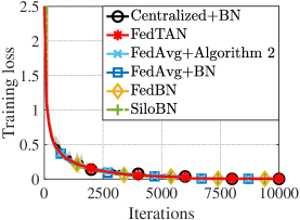
(a) i.i.d.

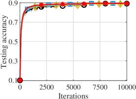
(b) i.i.d.

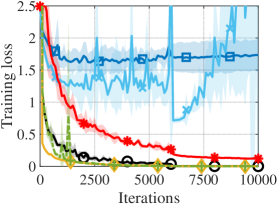
(c) Non-i.i.d.

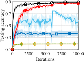
(d) Non-i.i.d.

Figure 4: Performance of different FL schemes on CIFAR-10 dataset. The mini-batch SGD without momentum or weight decay is adopted.

Table 1: Testing accuracy of different FL schemes on CIFAR-10 dataset. The mini-batch SGD with momentum and weight decay is adopted.

FL scheme	i.i.d. (%)	Non-i.i.d. (%)
Centralized+BN	91.53 $\pm$ 0.50	91.53 $\pm$ 0.50
FedTAN	91.26 $\pm$ 0.21	87.66 $\pm$ 0.43
FedAvg+BN	91.35 $\pm$ 0.24	45.90 $\pm$ 6.39
FedAvg+Algorithm 2	91.42 $\pm$ 0.15	76.01 $\pm$ 1.37
FedBN	90.74 $\pm$ 0.28	19.46 $\pm$ 0.05
SiloBN	91.31 $\pm$ 0.29	19.43 $\pm$ 0.09

Six baselines and a centralized learning scheme are considered for comparison with FedTAN.

• FedAvg+BN: This scheme uses the vanilla FedAvg algorithm to train ResNet-20 with BN.

• FedAvg+Algorithm 2: We consider a simplified implementation of FedDNA in [21] by assuming $\mathcal{S}_{\mathcal{D}_{i}}^{r,1}=\mathcal{S}_{\mathcal{D}}^{r,1}$, $\forall i\in[N]$. However, FedDNA does not consider the deviation $\Delta\mathcal{S}_{\mathcal{D}_{i}}^{r,1}\neq\Delta\mathcal{S}_{\mathcal{D}}^{r,1}$.

• FedBN [15]: This scheme updates all parameters in BN layers locally while uploading model coefficients in other layers to the server for global aggregation.

• SiloBN [18]: This scheme updates only the statistical parameters in BN locally while uploading all gradient parameters to the server for global aggregation.

• FedAvg+GN [16]: As an alternative to BN, GN is less sensitive to data distribution and is also widely used. This scheme employs FedAvg to train ResNet-20 with GN.

• SingleNet [15]: This scheme updates all parameters locally without exchanging any parameter with the server.

• Centralized+BN: In centralized learning, the global dataset is used to train ResNet-20 with BN, which serves as the performance upper bound in the simulations.

6.2 Robustness under Different Data Distributions

6.2.1 The i.i.d. data case

Fig. 4 compares the training loss and testing accuracy of different FL schemes on CIFAR-10 dataset by adopting mini-batch SGD without momentum or weight decay in local model updating. Each curve and filled area represent the mean and standard variance of five independent experimental results. FedBN and SiloBN, unlike FedAvg, keep part or all of BN parameters updating locally, and would possess different local models after global aggregation. Thus, we estimate the local training loss of each client in FedBN or SiloBN by its model and dataset, while assessing the generalization ability of each local model based on the 10000 samples in the CIFAR-10 testing dataset. Afterward, the training loss and testing accuracy of these two FL schemes are calculated by averaging the local results of all clients.

According to Fig. 4(a) and 4(b), in the i.i.d. data case, all FL schemes are comparable to the centralized learning method. Specifically, in the i.i.d. case, $\mathcal{S}_{\mathcal{D}_{i}}^{r,1}=\mathcal{S}_{\mathcal{D}}^{r,1}$ and $\Delta\mathcal{S}_{\mathcal{D}_{i}}^{r,1}=\Delta\mathcal{S}_{\mathcal{D}}^{r,1}$ are true as discussed in Property 1. As a result, the gradient deviation under BN $B_{i}=0$ in Theorem 1, and the learned model by FL with BN can converge in the right direction.

6.2.2 The non-i.i.d. data case

Comparing Fig. 4(a) and 4(b) with Fig. 4(c) and 4(d), we can find that the non-i.i.d. data damages the performance of all FL schemes, but the proposed FedTAN still performs closely to the centralized learning scheme and outperforms other FL benchmarks. Specifically, Fig. 4(c) and 4(d) show that both FedBN and SiloBN exhibit good training performance on the local datasets with only two classes of samples, even converging faster than the centralized learning scheme, but have poor testing performance on the entire testing dataset with ten classes of samples. This observation indicates that the DNN models learned by these two FL schemes are local optimal solutions and cannot be generalized. The reason for this is that FedBN assumes the clients possess i.i.d. label distributions, while SiloBN considers each client has all classes of samples locally, which does not hold in our setting on non-i.i.d. data. In addition, FedAvg+Algorithm 2 improves FL performance significantly over the vanilla FedAvg+BN, taking into account the mismatched statistical parameters. However, FedAvg+Algorithm 2 ignores the deviation $\Delta\mathcal{S}_{\mathcal{D}_{i}}^{r,1}\neq\Delta\mathcal{S}_{\mathcal{D}}^{r,1}$, and thus it fluctuates widely and still fails to converge to a satisfactory result. In contrast to the FL benchmarks above, through the layer-wise aggregations on statistical parameters in Algorithm 2 and on their gradients in Algorithm 3, FedTAN is capable of meeting the condition (38) to achieve superior performance.

We further demonstrate the effectiveness of proposed FedTAN by adopting mini-batch SGD with momentum and weight decay. Table 1 compares the testing accuracy of different FL schemes, based on the mean and standard deviation of five independent experiments. As can be observed, FedTAN performs well for both data cases, while other FL benchmarks significantly degrade in the non-i.i.d. data case. In particular, under the non-i.i.d. data, FedTAN increases its average testing accuracy by 41.76% compared to FedAvg+BN.

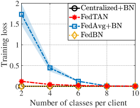
(a) Training loss.

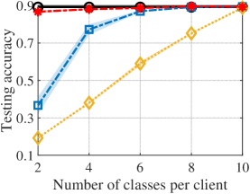
(b) Testing accuracy.

Figure 5: FL Performance on CIFAR-10 dataset with different distribution shifts. The mini-batch SGD without momentum or weight decay is adopted.

6.2.3 Influence of different distribution shifts

As mentioned in [41], a higher number of classes per client reduces distribution shifts among clients. Consequently, we adopt the data partition method from [41] and compare the FL performance under different numbers of classes per client, as illustrated in Fig. 5. The case with two classes per client corresponds to the considered (extremely) non-i.i.d. data scenario in Section 6.1, while ten classes per client represent the i.i.d. data case. Detailed class distributions for each case are provided in Section D of the Supplementary Material. Notably, FedTAN closely matches centralized learning in all cases. However, as the number of classes per client decreases, both FedAvg+BN and FedBN experience significant performance drops due to gradient deviation and poor generalization ability, respectively.

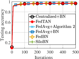
(a) i.i.d.

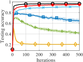
(b) Non-i.i.d.

Figure 6: Testing accuracy of different FL schemes on MNIST dataset.

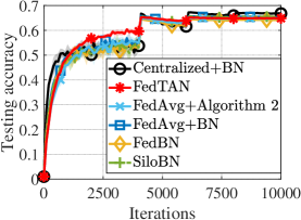
(a) i.i.d.

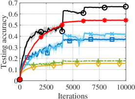
(b) Non-i.i.d.

Figure 7: Performance of different FL schemes on CIFAR-100 dataset.

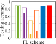
(a) Amazon.

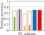
(b) Caltech.

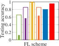
(c) DSLR.

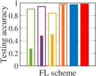
(d) Webcam.

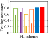
(e) Global.

Figure 8: Performance of different FL schemes on Office-Caltech10 dataset.

6.3 Adaptability under Different-Scale Datasets

To assess the adaptability of proposed FedTAN on datasets of varying scales, we further compare its performance on two additional datasets: MNIST with ten classes of images (Fig. 6), and CIFAR-100 with one hundred classes of images (Fig. 7). As shown in Fig. 6 and 7, similar to the previous CIFAR-10 experiment depicted in Fig. 4, FedTAN exhibits even closer performance to centralized learning in both the i.i.d. and non-i.i.d. data cases. Conversely, other FL baselines experience a significant performance drop in the non-i.i.d. data case.

6.4 Generalization Ability under Feature Shifts

In the non-i.i.d. case of previous experiments, clients have different label distributions for their local training samples. In this subsection, we use the Office-Caltech10 dataset to demonstrate how the proposed FedTAN effectively addresses another non-i.i.d. issue called feature shift [15]. Feature shift refers to a scenario where clients have the same label distributions but different feature distributions.

We denote FedBN-A, FedBN-C, FedBN-D, and FedBN-W as FedBN schemes updated by clients with local datasets from Amazon, Caltech, DSLR, and Webcam, respectively. The same notation applies to SingleNet variants. Fig. 8 compares the performance of various FL schemes on testing datasets from different data sources and the whole global testing dataset. It can be observed that FedBN outperforms SingleNet when the training and testing datasets come from different sources due to its improved generalization ability. However, FedBN would still perform worse when datasets have different sources, as seen in FedBN-D in Fig. 8(a) and FedBN-A in Fig. 8(c), because it updates all BN parameters locally. In contrast, FedTAN, with aggregated model parameters in the server, exhibits superior generalization ability and achieves satisfactory performance under each testing dataset. It proves more robust than FedAvg+BN, which suffers from gradient deviation, especially evident in Fig. 8(c). Additionally, we conduct experiments on training AlexNet using the DomainNet dataset [42], obtaining similar observations. See Section F in the Supplementary Material for details.

6.5 Comparison with Group Normalization

6.5.1 Learning performance

In comparison to BN, GN [13] is less sensitive to data distribution and also widely used. Despite this, GN is still unable to match the performance of BN in many recognition tasks. For instance, replacing BN with GN during ResNet training on the CIFAR dataset leads to performance degradation [43]. Based on CIFAR-10 dataset, Fig. 9 compares the performance of the ResNet-20 with BN trained by FedTAN and the one with GN trained by FedAvg, in terms of iterations. Additionally, Table 2 compares the testing accuracy of the global models obtained through these two schemes after the entire training process. It can be seen from Fig. 9 and Table 2 that, for both i.i.d. and non-i.i.d data cases, FedTAN maintains the superiority of BN and achieves higher testing accuracy with faster convergence rates. Furthermore, employing mini-batch SGD with momentum enhances the learning performance of both FedTAN and FedAvg+GN compared to the case without momentum.

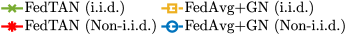
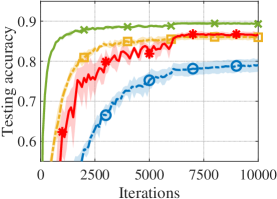
(a) Without momentum.

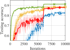
(b) With momentum.

Figure 9: Performance comparison between FedTAN and FedAvg+GN on CIFAR-10 dataset.

Table 2: Testing accuracy of FedTAN and FedAvg+GN on CIFAR-10 dataset.

FL scheme	Without momentum (%)		With momentum (%)
	i.i.d.	Non-i.i.d.	i.i.d.	Non-i.i.d.
FedTAN	89.32$\pm$0.28	86.69$\pm$0.82	91.26$\pm$0.21	87.66$\pm$0.43
FedAvg+GN	85.99$\pm$0.71	79.01$\pm$1.63	88.41$\pm$0.46	82.66$\pm$1.48

6.5.2 Communication overhead

In FedTAN, as depicted in Algorithms 1, 2 and 3, the modified first local updating step brings extra transmission of statistical parameters and their gradients between the server and the clients. Table 3 compares the number of bits exchanged between the server and five clients per iteration required by different FL schemes when training ResNet-20 with the CIFAR-10 dataset, where the detailed calculation process of each exchanged data volume is provided in Section G of the Supplementary Material. Table 3 shows that, compared to FedAvg+BN and FedAvg+GN, the transmitted data volume between the server and clients in FedTAN only increases by 1.02% and 1.52%, respectively. This slight increase is due to statistical parameters comprising a small portion of all parameters, especially in large-scale DNNs. Next, Fig. 10 compares the testing accuracy of various FL schemes concerning the number of bits exchanged between the server and all clients. The figure shows that with negligible additional exchanged bits, FedTAN is still capable of maintaining the faster convergence rate w.r.t. the transmission data volume. Specifically, given an expected level of testing accuracy, FedAvg+GN requires significantly more bits to be exchanged between the server and clients due to its slower convergence rate compared to FedTAN. Moreover, while FedTAN achieves higher learning accuracy, the extra communication rounds caused by the layer-wise aggregations in Algorithms 2 and 3 will increase the total communication rounds required for FedTAN. Thus, FedAvg+GN is recommended if the number of communication rounds is critical.

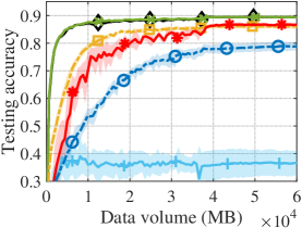
(a) Without momentum.

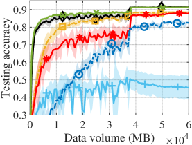
(b) With momentum.

Figure 10: FL Performance w.r.t. exchanged bits on CIFAR-10 dataset.

Table 3: Communication overhead per iteration of FL schemes on CIFAR-10 dataset.

FL scheme	Exchanged bits	Percentage higher than
	(MB)	FedAvg+BN	FedAvg+GN
FedTAN	6.2679	1.02%	1.52%
FedAvg+BN	6.2049	0	0.51%
FedAvg+GN	6.1734	-0.51%	0

6.6 Performance of FedTAN-II

Finally, we demonstrate the effectiveness of FedTAN-II. Fig. 11(a) and (b) compare FedTAN-II with FedTAN by training ResNet-20 with BN on the CIFAR-10 dataset in terms of iterations, while Fig. 11(c) and (d) compare them in terms of communication rounds. In the case of FedTAN-II, we initially set the learning rate $\gamma$ to 0.5 during the first $M$ iterations, similar to FedTAN, as mentioned in Section 6.1. After $M$ iterations, we adjust the learning rate $\gamma$ since we only update the gradient parameters while keeping the statistical parameters in BN layers fixed. Consequently, $\gamma$ is decreased to 0.01 and 0.001 after $M$ and 6000 iterations, respectively. If momentum ($0.9$) and weight decay ($10^{-4}$) are used in mini-batch SGD, $\gamma$ is further reduced to 0.0001 after 8000 iterations.

From Fig. 11, we observe that reducing $M$ leads to a slight accuracy loss if $M$ is smaller than a certain value (e.g., $M\leq 2000$ in Fig. 11(a) and $M\leq 1000$ in Fig. 11(c)), primarily due to less accurate statistical parameters. However, a smaller $M$ significantly reduces the required communication rounds, as shown in Fig. 11(b) and (d). Furthermore, a comparison between Fig. 11(a) and (c) reveals that adopting mini-batch SGD with momentum and weight decay greatly improves the testing accuracy of FedTAN-II under different $M$.

Next, Table 4 compares the total exchanged bits, the percentages of extra communication rounds and exchanged bits caused by layer-aggregations in Algorithms 2 and 3 during the entire training process of FedTAN-II for varying values of $M$. The table shows that the difference in total exchanged bits between FedTAN and FedTAN-II under different $M$ is negligible, as the statistical parameters in BN layers occupy only a small portion of the total model size. Moreover, we find that although the extra communication rounds caused by layer-aggregations in Algorithms 2 and 3 account for a large percentage of the total exchanged rounds during the entire training process, the corresponding extra exchanged bits are negligible. Thus, the layer-aggregations in Algorithms 2 and 3 constitute a high-frequent low-volume communication mode, which effectively mitigates divergence among local models, as highlighted in [7].

Additionally, we carry out experiments involving the training of a 3-layer DNN with BN on the MNIST dataset, leading to consistent observations. See Section H in the Supplementary Material for details.

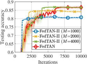
(a) Without momentum.

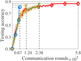
(b) Without momentum.

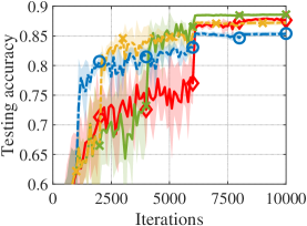
(c) With momentum.

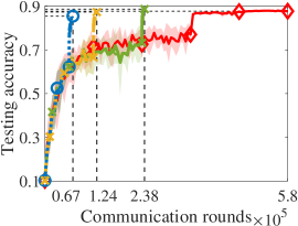
(d) With momentum.

Figure 11: Testing accuracy of FedTAN-II on CIFAR-10 dataset.

Table 4: Communication overhead of FedTAN-II on CIFAR-10 dataset.

FL scheme	Exchanged	Percentage of extra
	bits (GB)	Rounds	Bits
FedTAN-II ($M$$=$1000)	60.6563	85.07%	0.1014%
FedTAN-II ($M$$=$2000)	60.7178	91.94%	0.2027%
FedTAN-II ($M$$=$4000)	60.8408	95.80%	0.4045%
FedTAN	61.2100	98.28%	1.0051%

7 Conclusion

In this paper, we have investigated why BN damages the performance of FL in the non-i.i.d. data case. Our novel convergence analysis has revealed that BN significantly hinders the FL convergence in the presence of non-i.i.d. data. Specifically, we have shown that non-i.i.d. data would result in two types of mismatches: one between local and global statistical parameters and the other between the associated gradients w.r.t. the statistical parameters. These mismatches lead to gradient deviation in local models, which subsequently biases the FL convergence (Theorem 1). Fortunately, the gradient deviation can be eliminated if the local statistical parameters and related gradients, obtained by clients in the first local updating step, are the same as the global ones obtained by the centralized learning scheme. Inspired by this insight, we have proposed FedTAN, which leverages layer-wise statistical parameter aggregation to address the aforementioned mismatches and mitigate gradient deviation. The experimental results have showcased that, compared to existing schemes, FedTAN preserves the training advantage of BN while exhibiting superior robustness, particularly in non-i.i.d. data settings. Moreover, although layer-wise aggregation in FedTAN leads to a negligible increase in transmitted data volume, it does introduce a noticeable rise in communication rounds. To tackle this challenge, we have proposed FedTAN-II, which achieves satisfactory learning performance while significantly reducing the communication rounds.

Appendix

Appendix A Proof of Theorem 1

A.1 Proof of Convergence Rate

Based on Assumption 3, we have

$$F({\bar{\mathbf{w}}}_{r};\mathcal{S}_{\mathcal{D}}^{r+1,1},\Delta\mathcal{S}_{\mathcal{D}}^{r+1,1})\leq F({\bar{\mathbf{w}}}_{r-1};\mathcal{S}_{\mathcal{D}}^{r,1},\Delta\mathcal{S}_{\mathcal{D}}^{r,1})+\langle\nabla_{\mathbf{w}}F({\bar{\mathbf{w}}}_{r-1};\mathcal{S}_{\mathcal{D}}^{r,1},\Delta\mathcal{S}_{\mathcal{D}}^{r,1}),{\bar{\mathbf{w}}}_{r}-{\bar{\mathbf{w}}}_{r-1}\rangle+\frac{L}{2}\|{\bar{\mathbf{w}}}_{r}-{\bar{\mathbf{w}}}_{r-1}\|^{2},$$ (42)

where $\mathcal{S}_{\mathcal{D}}^{r,1}$ and $\Delta\mathcal{S}_{\mathcal{D}}^{r,1}$ are obtained via (2) with ${\bar{\mathbf{w}}}_{r-1}$ and the global dataset $\mathcal{D}$. Then, based on (42), we use the following three key lemmas which are proved in subsequent subsections.

Lemma 1

Under Assumptions 1 and 3, it holds that

$$\langle\nabla_{\mathbf{w}}F({\bar{\mathbf{w}}}_{r-1};\mathcal{S}_{\mathcal{D}}^{r,1},\Delta\mathcal{S}_{\mathcal{D}}^{r,1}),{\bar{\mathbf{w}}}_{r}-{\bar{\mathbf{w}}}_{r-1}\rangle\leq -\frac{\gamma E}{2}\big{\|}\nabla_{\mathbf{w}}F({\bar{\mathbf{w}}}_{r-1};\mathcal{S}_{\mathcal{D}}^{r,1},\Delta\mathcal{S}_{\mathcal{D}}^{r,1})\big{\|}^{2}\!-\!\frac{\gamma}{2}\sum_{t=1}^{E}\left\|\sum_{i=1}^{N}p_{i}\nabla_{\mathbf{w}}F_{i}(\mathbf{w}^{r,t-1}_{i};\mathcal{S}_{\mathcal{D}_{i}}^{r,t},\Delta\mathcal{S}_{\mathcal{D}_{i}}^{r,t})\right\|^{2}$$

$$+\gamma E\sum_{i=1}^{N}p_{i}B_{i}^{2}+\gamma L^{2}\sum_{i=1}^{N}p_{i}\sum_{t=1}^{E}\left\|\mathbf{w}^{r,t-1}_{i}-\mathbf{\bar{w}}_{r-1}\right\|^{2},$$ (43)

where $\mathcal{S}_{\mathcal{D}_{i}}^{r,t}$ and $\Delta\mathcal{S}_{\mathcal{D}_{i}}^{r,t}$ are obtained via (2) with $\mathbf{w}^{r,t-1}_{i}$ and the local dataset $\mathcal{D}_{i}$.

Lemma 2

With (5) and (7), we have

$${\bar{\mathbf{w}}}_{r}-{\bar{\mathbf{w}}}_{r-1}=-\gamma\sum_{t=1}^{E}\sum_{i=1}^{N}p_{i}\nabla_{\mathbf{w}}F_{i}(\mathbf{w}^{r,t-1}_{i};\mathcal{S}_{\mathcal{D}_{i}}^{r,t},\Delta\mathcal{S}_{\mathcal{D}_{i}}^{r,t}),$$ (44)

which results in

$$\left\|{\bar{\mathbf{w}}}_{r}-{\bar{\mathbf{w}}}_{r-1}\right\|^{2}\leq\gamma^{2}E\sum_{t=1}^{E}\bigg{\|}\sum_{i=1}^{N}p_{i}\nabla_{\mathbf{w}}F_{i}(\mathbf{w}^{r,t-1}_{i};\mathcal{S}_{\mathcal{D}_{i}}^{r,t},\Delta\mathcal{S}_{\mathcal{D}_{i}}^{r,t})\bigg{\|}^{2}.$$ (45)

Lemma 3

Under Assumptions 3 and 4, the difference between the local model at each round $r$ and the global model at the previous round is bounded by

$$\sum_{t=1}^{E}\left\|\mathbf{w}^{r,t-1}_{i}-{\bar{\mathbf{w}}}_{r-1}\right\|^{2}\leq\frac{4\gamma^{2}E^{3}B_{i}^{2}+4\gamma^{2}E^{3}V_{i}^{2}}{1-4\gamma^{2}E^{2}L^{2}}+\frac{4\gamma^{2}E^{3}\big{\|}\nabla_{\mathbf{w}}F(\mathbf{\bar{w}}_{r-1};\mathcal{S}_{\mathcal{D}}^{r,1},\Delta\mathcal{S}_{\mathcal{D}}^{r,1})\big{\|}^{2}}{1-4\gamma^{2}E^{2}L^{2}}.$$ (46)

Then, by substituting (1) into the third term in the RHS of (42) and substituting (45) into the second term, we have

$$F({\bar{\mathbf{w}}}_{r};\mathcal{S}_{\mathcal{D}}^{r+1,1},\Delta\mathcal{S}_{\mathcal{D}}^{r+1,1})$$

$$\leq F({\bar{\mathbf{w}}}_{r-1};\mathcal{S}_{\mathcal{D}}^{r,1},\Delta\mathcal{S}_{\mathcal{D}}^{r,1})-\frac{\gamma E}{2}\big{\|}\nabla_{\mathbf{w}}F({\bar{\mathbf{w}}}_{r-1};\mathcal{S}_{\mathcal{D}}^{r,1},\Delta\mathcal{S}_{\mathcal{D}}^{r,1})\big{\|}^{2}-\frac{\gamma(1-\gamma EL)}{2}\sum_{t=1}^{E}\left\|\sum_{i=1}^{N}p_{i}\nabla_{\mathbf{w}}F_{i}(\mathbf{w}^{r,t-1}_{i};\mathcal{S}_{\mathcal{D}_{i}}^{r,t},\Delta\mathcal{S}_{\mathcal{D}_{i}}^{r,t})\right\|^{2}$$

$$+\gamma E\sum_{i=1}^{N}p_{i}B_{i}^{2}+\gamma L^{2}\sum_{i=1}^{N}p_{i}\sum_{t=1}^{E}\left\|\mathbf{w}^{r,t-1}_{i}-\mathbf{\bar{w}}_{r-1}\right\|^{2}$$

$$\overset{(a)}{\leq} F({\bar{\mathbf{w}}}_{r-1};\mathcal{S}_{\mathcal{D}}^{r,1},\Delta\mathcal{S}_{\mathcal{D}}^{r,1})-\frac{\gamma E}{2}\big{\|}\nabla_{\mathbf{w}}F({\bar{\mathbf{w}}}_{r-1};\mathcal{S}_{\mathcal{D}}^{r,1},\Delta\mathcal{S}_{\mathcal{D}}^{r,1})\big{\|}^{2}+\gamma E\sum_{i=1}^{N}p_{i}B_{i}^{2}+\gamma L^{2}\sum_{i=1}^{N}p_{i}\sum_{t=1}^{E}\left\|\mathbf{w}^{r,t-1}_{i}-\mathbf{\bar{w}}_{r-1}\right\|^{2},$$ (47)

where (a) is obtained by setting $0<\gamma\leq\frac{1}{EL}$.

Next, by substituting (46) into the last term of (A.1), we have

$$F({\bar{\mathbf{w}}}_{r};\mathcal{S}_{\mathcal{D}}^{r+1,1},\Delta\mathcal{S}_{\mathcal{D}}^{r+1,1})\leq F({\bar{\mathbf{w}}}_{r-1};\mathcal{S}_{\mathcal{D}}^{r,1},\Delta\mathcal{S}_{\mathcal{D}}^{r,1})-\left(\frac{\gamma E}{2}-\frac{4\gamma^{3}E^{3}L^{2}}{1-4\gamma^{2}E^{2}L^{2}}\right)\big{\|}\nabla_{\mathbf{w}}F({\bar{\mathbf{w}}}_{r-1};\mathcal{S}_{\mathcal{D}}^{r,1},\Delta\mathcal{S}_{\mathcal{D}}^{r,1})\big{\|}^{2}$$

$$+\frac{4\gamma^{3}E^{3}L^{2}}{1-4\gamma^{2}E^{2}L^{2}}\sum_{i=1}^{N}p_{i}V_{i}^{2}+\frac{4\gamma^{3}E^{3}L^{2}}{1-4\gamma^{2}E^{2}L^{2}}\sum_{i=1}^{N}p_{i}B_{i}^{2}+\gamma E\sum_{i=1}^{N}p_{i}B_{i}^{2}\text{.}$$ (48)

After that, summing the above items from ${r}=1$ to $R$ and dividing both sides by the multiplication of the learning rate and the total number of local mini-batch SGD steps, $\gamma T(=\gamma RE)$, yields

$$\underbrace{\left(\frac{1}{2}-\frac{4\gamma^{2}E^{2}L^{2}}{1-4\gamma^{2}E^{2}L^{2}}\right)}_{\triangleq H_{1}}\frac{\sum_{r=1}^{R}\|\nabla_{\mathbf{w}}F({\bar{\mathbf{w}}}_{r-1};\mathcal{S}_{\mathcal{D}}^{r,1},\Delta\mathcal{S}_{\mathcal{D}}^{r,1})\|^{2}}{R}$$

$$\leq \underbrace{\frac{1}{\gamma T}}_{\triangleq H_{2}}\Big{(}F({\bar{\mathbf{w}}}_{0};\mathcal{S}_{\mathcal{D}}^{1,1},\Delta\mathcal{S}_{\mathcal{D}}^{1,1})-F({\bar{\mathbf{w}}}_{R};\mathcal{S}_{\mathcal{D}}^{R+1,1},\Delta\mathcal{S}_{\mathcal{D}}^{R+1,1})\Big{)}+\underbrace{\frac{4\gamma^{2}E^{2}L^{2}}{1-4\gamma^{2}E^{2}L^{2}}}_{\triangleq H_{3}}\sum_{i=1}^{N}p_{i}V_{i}^{2}+\underbrace{\frac{4\gamma^{2}E^{2}L^{2}}{1-4\gamma^{2}E^{2}L^{2}}}_{\triangleq H_{3}}\sum_{i=1}^{N}p_{i}B_{i}^{2}+\sum_{i=1}^{N}p_{i}B_{i}^{2}\text{.}$$ (49)

Let the learning rate $\gamma=N^{\frac{1}{2}}/(4L{T}^{\frac{1}{2}})$ and the number of local updating steps $E\leq T^{\frac{1}{4}}/N^{\frac{3}{4}}$, where $T\geq N^{3}$ in order to ensure $E\geq 1$. By this, the condition $0<\gamma\leq\frac{1}{EL}$ in (A.1) can be satisfied, and $H_{2}=4L(TN)^{-\frac{1}{2}}$. Next, since $\gamma EL\leq(TN)^{-\frac{1}{4}}/4$, we have

$$H_{3}\leq\frac{\frac{4}{4^{2}}(TN)^{-\frac{1}{2}}}{1-\frac{4}{4^{2}}(TN)^{-\frac{1}{2}}}\overset{(a)}{\leq}\frac{\frac{4}{4^{2}}(TN)^{-\frac{1}{2}}}{1-\frac{4}{4^{2}}}=\frac{1}{3(TN)^{\frac{1}{2}}},$$ (50)

where inequality (a) is due to $T\geq 1$ and $N\geq 1$. Then,

$$H_{1}=\frac{1}{2}-H_{3}\geq\frac{1}{2}-\frac{1}{3(TN)^{\frac{1}{2}}}\geq\frac{1}{2}-\frac{1}{3}=\frac{1}{6}\,.$$ (51)

Finally, by substituting above coefficients and $F({\bar{\mathbf{w}}}_{R};$ $\mathcal{S}_{\mathcal{D}}^{R+1,1},\Delta\mathcal{S}_{\mathcal{D}}^{R+1,1})\geq\underline{F}$ in Assumption 2 into (A.1), Theorem 1 is proved.

$\blacksquare$

A.2 Proof of Lemma 1

Based on (44), we have

$$\langle\nabla_{\mathbf{w}}F({\bar{\mathbf{w}}}_{r-1};\mathcal{S}_{\mathcal{D}}^{r,1},\Delta\mathcal{S}_{\mathcal{D}}^{r,1}),{\bar{\mathbf{w}}}_{r}-{\bar{\mathbf{w}}}_{r-1}\rangle$$

$$= \Big{\langle}\nabla_{\mathbf{w}}F({\bar{\mathbf{w}}}_{r-1};\mathcal{S}_{\mathcal{D}}^{r,1},\Delta\mathcal{S}_{\mathcal{D}}^{r,1}),-\gamma\sum_{t=1}^{E}\sum_{i=1}^{N}p_{i}\nabla_{\mathbf{w}}F_{i}(\mathbf{w}^{r,t-1}_{i};\mathcal{S}_{\mathcal{D}_{i}}^{r,t},\Delta\mathcal{S}_{\mathcal{D}_{i}}^{r,t})\Big{\rangle}$$

$$= -\gamma\sum_{t=1}^{E}\Big{\langle}\nabla_{\mathbf{w}}F({\bar{\mathbf{w}}}_{r-1};\mathcal{S}_{\mathcal{D}}^{r,1},\Delta\mathcal{S}_{\mathcal{D}}^{r,1}),\sum_{i=1}^{N}p_{i}\nabla_{\mathbf{w}}F_{i}(\mathbf{w}^{r,t-1}_{i};\mathcal{S}_{\mathcal{D}_{i}}^{r,t},\Delta\mathcal{S}_{\mathcal{D}_{i}}^{r,t})\Big{\rangle}$$

$$\overset{(a)}{=} -\frac{\gamma E}{2}\big{\|}\nabla_{\mathbf{w}}F({\bar{\mathbf{w}}}_{r-1};\mathcal{S}_{\mathcal{D}}^{r,1},\Delta\mathcal{S}_{\mathcal{D}}^{r,1})\big{\|}^{2}-\frac{\gamma}{2}\sum_{t=1}^{E}\bigg{\|}\sum_{i=1}^{N}p_{i}\nabla_{\mathbf{w}}F_{i}(\mathbf{w}^{r,t-1}_{i};\mathcal{S}_{\mathcal{D}_{i}}^{r,t},\Delta\mathcal{S}_{\mathcal{D}_{i}}^{r,t})\bigg{\|}^{2}$$

$$+\frac{\gamma}{2}\sum_{t=1}^{E}\bigg{\|}\nabla_{\mathbf{w}}F({\bar{\mathbf{w}}}_{r-1};\mathcal{S}_{\mathcal{D}}^{r,1},\Delta\mathcal{S}_{\mathcal{D}}^{r,1})-\sum_{i=1}^{N}p_{i}\nabla_{\mathbf{w}}F_{i}({\bar{\mathbf{w}}}_{r-1};\mathcal{S}_{\mathcal{D}_{i}}^{r,1},\Delta\mathcal{S}_{\mathcal{D}_{i}}^{r,1})$$

$$\qquad\qquad\;\;+\sum_{i=1}^{N}p_{i}\nabla_{\mathbf{w}}F_{i}({\bar{\mathbf{w}}}_{r-1};\mathcal{S}_{\mathcal{D}_{i}}^{r,1},\Delta\mathcal{S}_{\mathcal{D}_{i}}^{r,1})-\sum_{i=1}^{N}p_{i}\nabla_{\mathbf{w}}F_{i}(\mathbf{w}^{r,t-1}_{i};\mathcal{S}_{\mathcal{D}_{i}}^{r,t},\Delta\mathcal{S}_{\mathcal{D}_{i}}^{r,t})\bigg{\|}^{2}$$

$$\overset{(b)}{\leq} -\frac{\gamma}{2}\sum_{t=1}^{E}\left\|\nabla_{\mathbf{w}}F({\bar{\mathbf{w}}}_{r-1};\mathcal{S}_{\mathcal{D}}^{r,1},\Delta\mathcal{S}_{\mathcal{D}}^{r,1})\right\|^{2}-\frac{\gamma}{2}\sum_{t=1}^{E}\bigg{\|}\sum_{i=1}^{N}p_{i}\nabla_{\mathbf{w}}F_{i}(\mathbf{w}^{r,t-1}_{i};\mathcal{S}_{\mathcal{D}_{i}}^{r,t},\Delta\mathcal{S}_{\mathcal{D}_{i}}^{r,t})\bigg{\|}^{2}$$

$$+\gamma E\underbrace{\bigg{\|}\nabla_{\mathbf{w}}F({\bar{\mathbf{w}}}_{r-1};\mathcal{S}_{\mathcal{D}}^{r,1},\Delta\mathcal{S}_{\mathcal{D}}^{r,1})-\sum_{i=1}^{N}p_{i}\nabla_{\mathbf{w}}F_{i}({\bar{\mathbf{w}}}_{r-1};\mathcal{S}_{\mathcal{D}_{i}}^{r,1},\Delta\mathcal{S}_{\mathcal{D}_{i}}^{r,1})\bigg{\|}^{2}}_{\triangleq A_{1}}$$

$$+\gamma\sum_{t=1}^{E}\underbrace{\bigg{\|}\sum_{i=1}^{N}p_{i}\Big{(}\nabla_{\mathbf{w}}F_{i}({\bar{\mathbf{w}}}_{r-1};\mathcal{S}_{\mathcal{D}_{i}}^{r,1},\Delta\mathcal{S}_{\mathcal{D}_{i}}^{r,1})-\nabla_{\mathbf{w}}F_{i}(\mathbf{w}^{r,t-1}_{i};\mathcal{S}_{\mathcal{D}_{i}}^{r,t},\Delta\mathcal{S}_{\mathcal{D}_{i}}^{r,t})\Big{)}\bigg{\|}^{2}}_{\triangleq A_{2}}\text{,}$$ (52)

where equality (a) follows the basic identity $\langle{\mathbf{x}}_{1},{\mathbf{x}}_{2}\rangle=\frac{1}{2}(\|{\mathbf{x}}_{1}\|^{2}+\|{\mathbf{x}}_{2}\|^{2}-\|{\mathbf{x}}_{1}-{\mathbf{x}}_{2}\|^{2})$, inequality (b) is due to $\|x_{1}+x_{2}\|^{2}\leq 2\|x_{1}\|^{2}+2\|x_{2}\|^{2}$, and $A_{1}$ in equality (b) is bounded by

$$A_{1}\overset{(a)}{=} \Big{\|}\sum_{i=1}^{N}p_{i}\nabla_{\mathbf{w}}F_{i}({\bar{\mathbf{w}}}_{r-1};\mathcal{S}_{\mathcal{D}}^{r},\Delta\mathcal{S}_{\mathcal{D}}^{r})-\sum_{i=1}^{N}p_{i}\nabla_{\mathbf{w}}F_{i}({\bar{\mathbf{w}}}_{r-1};\mathcal{S}_{\mathcal{D}_{i}}^{r},\Delta\mathcal{S}_{\mathcal{D}_{i}}^{r})\Big{\|}^{2}$$

$$\overset{(b)}{\leq} \sum_{i=1}^{N}p_{i}\big{\|}\nabla_{\mathbf{w}}F_{i}({\bar{\mathbf{w}}}_{r-1};\mathcal{S}_{\mathcal{D}}^{r},\Delta\mathcal{S}_{\mathcal{D}}^{r})-\nabla_{\mathbf{w}}F_{i}({\bar{\mathbf{w}}}_{r-1};\mathcal{S}_{\mathcal{D}_{i}}^{r},\Delta\mathcal{S}_{\mathcal{D}_{i}}^{r})\big{\|}^{2}\overset{(c)}{\leq}\sum_{i=1}^{N}p_{i}B_{i}^{2}\,\text{,}$$ (53)

where equality (a) comes from (9), inequality (b) is by Jensen’s Inequality, and inequality (c) is obtained from Assumption 1. Meanwhile, we can bound $A_{2}$ as

$$A_{2}\overset{(a)}{\leq} \sum_{i=1}^{N}p_{i}\big{\|}\nabla_{\mathbf{w}}F_{i}({\bar{\mathbf{w}}}_{r-1};\mathcal{S}_{\mathcal{D}_{i}}^{r,1},\Delta\mathcal{S}_{\mathcal{D}_{i}}^{r,1})\!-\!\nabla_{\mathbf{w}}F_{i}(\mathbf{w}^{r,t-1}_{i};\mathcal{S}_{\mathcal{D}_{i}}^{r,t},\Delta\mathcal{S}_{\mathcal{D}_{i}}^{r,t})\big{\|}^{2}\overset{(b)}{\leq}L^{2}\sum_{i=1}^{N}p_{i}\big{\|}\mathbf{w}^{r,t-1}_{i}\!-\!\mathbf{\bar{w}}_{r-1}\big{\|}^{2},$$ (54)

where inequality (a) is due to Jensen’s Inequality and inequality (b) is obtained from Assumption 3. Finally, by substituting (A.2) and (54) into (A.2), we can obtain Lemma 1 directly. $\blacksquare$

A.3 Proof of Lemma 3

Based on (5), at the $r$-th iteration, local gradient parameters obtained by client $i\in[N]$ in the $t$-th local updating step are

$$\mathbf{w}_{i}^{r,t-1}=\mathbf{\bar{w}}_{r-1}-\gamma\sum_{e=1}^{t-1}\nabla_{\mathbf{w}}F_{i}(\mathbf{w}_{i}^{r,e-1};\mathcal{S}_{\mathcal{D}_{i}}^{r,e},\Delta\mathcal{S}_{\mathcal{D}_{i}}^{r,e})\,\text{.}$$ (55)

Therefore,

$$\big{\|}\mathbf{w}^{r,t-1}_{i}-{\bar{\mathbf{w}}}_{r-1}\big{\|}^{2}$$

$$= \Big{\|}\gamma\sum_{e=1}^{t-1}\nabla_{\mathbf{w}}F_{i}(\mathbf{w}_{i}^{r,e-1};\mathcal{S}_{\mathcal{D}_{i}}^{e,t},\Delta\mathcal{S}_{\mathcal{D}_{i}}^{e,t})\Big{\|}^{2}$$

$$\leq \gamma^{2}(t-1)\sum_{e=1}^{t-1}\big{\|}\nabla_{\mathbf{w}}F_{i}(\mathbf{w}_{i}^{r,e-1};\mathcal{S}_{\mathcal{D}_{i}}^{e,t},\Delta\mathcal{S}_{\mathcal{D}_{i}}^{e,t})\big{\|}^{2}\leq\gamma^{2}E\sum_{e=1}^{t-1}\big{\|}\nabla_{\mathbf{w}}F_{i}(\mathbf{w}_{i}^{r,e-1};\mathcal{S}_{\mathcal{D}_{i}}^{e,t},\Delta\mathcal{S}_{\mathcal{D}_{i}}^{e,t})\big{\|}^{2}$$

$$\leq 4\gamma^{2}E\sum_{e=1}^{t-1}\bigg{(}\big{\|}\nabla_{\mathbf{w}}F_{i}(\mathbf{w}_{i}^{r,e-1};\mathcal{S}_{\mathcal{D}_{i}}^{e,t},\Delta\mathcal{S}_{\mathcal{D}_{i}}^{e,t})-\nabla_{\mathbf{w}}F_{i}(\mathbf{\bar{w}}_{r-1};\mathcal{S}_{\mathcal{D}_{i}}^{r,1},\Delta\mathcal{S}_{\mathcal{D}_{i}}^{r,1})\big{\|}^{2}$$

$$\qquad\qquad\quad+\big{\|}\nabla_{\mathbf{w}}F_{i}(\mathbf{\bar{w}}_{r-1};\mathcal{S}_{\mathcal{D}_{i}}^{r,1},\Delta\mathcal{S}_{\mathcal{D}_{i}}^{r,1})-\nabla_{\mathbf{w}}F_{i}(\mathbf{\bar{w}}_{r-1};\mathcal{S}_{\mathcal{D}}^{r,1},\Delta\mathcal{S}_{\mathcal{D}}^{r,1})\big{\|}^{2}$$

$$\qquad\qquad\quad+\big{\|}\nabla_{\mathbf{w}}F_{i}(\mathbf{\bar{w}}_{r-1};\mathcal{S}_{\mathcal{D}}^{r,1},\Delta\mathcal{S}_{\mathcal{D}}^{r,1})-\nabla_{\mathbf{w}}F(\mathbf{\bar{w}}_{r-1};\mathcal{S}_{\mathcal{D}}^{r,1},\Delta\mathcal{S}_{\mathcal{D}}^{r,1})\big{\|}^{2}+\big{\|}\nabla_{\mathbf{w}}F(\mathbf{\bar{w}}_{r-1};\mathcal{S}_{\mathcal{D}}^{r,1},\Delta\mathcal{S}_{\mathcal{D}}^{r,1})\big{\|}^{2}\bigg{)}$$

$$\overset{(a)}{\leq} 4\gamma^{2}EL^{2}\sum_{e=1}^{t-1}\big{\|}\mathbf{w}_{i}^{r,e-1}-\mathbf{\bar{w}}_{r-1}\big{\|}^{2}+4\gamma^{2}E^{2}B_{i}^{2}+4\gamma^{2}E^{2}V_{i}^{2}+4\gamma^{2}E^{2}\big{\|}\nabla_{\mathbf{w}}F(\mathbf{\bar{w}}_{r-1};\mathcal{S}_{\mathcal{D}}^{r,1},\Delta\mathcal{S}_{\mathcal{D}}^{r,1})\big{\|}^{2},$$ (56)

where inequality (a) is obtained from Assumptions 1, 3 and 4. Then, summing both sides of (A.3) from $t=1$ to $E$ yields

$$\sum_{t=1}^{E}\big{\|}\mathbf{w}^{r,t-1}_{i}-{\bar{\mathbf{w}}}_{r-1}\big{\|}^{2}$$

$$\leq 4\gamma^{2}EL^{2}\underbrace{\sum_{t=1}^{E}\sum_{e=1}^{t-1}\big{\|}\mathbf{w}_{i}^{r,e-1}-\mathbf{\bar{w}}_{r-1}\big{\|}^{2}}_{\triangleq A_{3}}+4\gamma^{2}E^{3}B_{i}^{2}+4\gamma^{2}E^{3}V_{i}^{2}+4\gamma^{2}E^{3}\big{\|}\nabla_{\mathbf{w}}F(\mathbf{\bar{w}}_{r-1};\mathcal{S}_{\mathcal{D}}^{r,1},\Delta\mathcal{S}_{\mathcal{D}}^{r,1}))\big{\|}^{2}$$

$$\overset{(a)}{\leq} 4\gamma^{2}E^{2}L^{2}\sum_{t=1}^{E}\big{\|}\mathbf{w}_{i}^{r,t-1}-\mathbf{\bar{w}}_{r-1}\big{\|}^{2}+4\gamma^{2}E^{3}B_{i}^{2}+4\gamma^{2}E^{3}V_{i}^{2}+4\gamma^{2}E^{3}\big{\|}\nabla_{\mathbf{w}}F(\mathbf{\bar{w}}_{r-1};\mathcal{S}_{\mathcal{D}}^{r,1},\Delta\mathcal{S}_{\mathcal{D}}^{r,1}))\big{\|}^{2}\text{,}$$ (57)

where inequality (a) is because the occurrence number of $\|\mathbf{w}^{r,t-1}_{i}-{\bar{\mathbf{w}}}_{r-1}\|^{2}$ for each $t\in[1,E]$ in term $A_{3}$ is less than the number of local updating steps $E$, and then $A_{3}\leq E\sum_{t=1}^{E}\|\mathbf{w}_{i}^{r,t-1}-\mathbf{\bar{w}}_{r-1}\|^{2}$.

Finally, rearranging the terms in (A.3) yields Lemma 3. $\blacksquare$

Supplementary Material

Appendix A Derivation of (28)

Based on (1) and the chain rule, the local gradient w.r.t. the batch mean in the last BN layer obtained by client $i\in[N]$ in FL is

$${\nabla}_{\bm{\mu}_{i}^{L}}{F_{i}}={\nabla}_{\mathbf{\hat{Y}}_{i}^{L}}{F_{i}}\cdot{\nabla}_{\bm{\mu}_{i}^{L}}{\mathbf{\hat{Y}}_{i}^{L}}+{\nabla}_{(\bm{\sigma}_{i}^{L})^{2}}{F_{i}}\cdot{\nabla}_{\bm{\mu}_{i}^{L}}{(\bm{\sigma}_{i}^{L})^{2}}$$ (58)

where

$${\nabla}_{\bm{\mu}_{i}^{L}}{(\bm{\sigma}_{i}^{L})^{2}}\overset{(a)}{=}\operatorname{diag}\bigg{(}\sum_{c}\bigg{(}\int 2(\bm{\mu}_{i}^{L}-\mathbf{y}^{L})\cdot f_{{\mathbf{Y}_{i}^{L}}|{\mathbf{X}_{i}^{0}}}(\mathbf{y}^{L}|{\mathbf{x}^{0}}\in c)\cdot d\mathbf{y}^{L}\bigg{)}\cdot\Pr(c|\mathcal{D}_{i})\bigg{)}\overset{(b)}{=}\operatorname{diag}(\mathbf{0}),$$ (59)

where equalities (a) and (b) are based on (2) and (19a). Thus, by substituting (59) into (58), we have

$${\nabla}_{\bm{\mu}_{i}^{L}}{F_{i}}= \underbrace{{\nabla}_{\mathbf{Y}_{i}^{L+1}}{F_{i}}\cdot{\nabla}_{\mathbf{X}_{i}^{L}}{\mathbf{Y}_{i}^{L+1}}\cdot{\nabla}_{\mathbf{\hat{Y}}_{i}^{L}}{\mathbf{X}_{i}^{L}}}_{={\nabla}_{\mathbf{\hat{Y}}_{i}^{L}}{F_{i}}}\cdot{\nabla}_{(\bm{\mu}_{i}^{L})^{2}}{\mathbf{\hat{Y}}_{i}^{L}}=\mathbb{E}_{\mathcal{D}_{i}}\Big{[}{\nabla}_{\mathbf{Y}_{i}^{L+1}}{\mathcal{L}_{i}}\cdot{\nabla}_{\mathbf{X}_{i}^{L}}{\mathbf{Y}_{i}^{L+1}}\cdot{\nabla}_{\mathbf{\hat{Y}}_{i}^{L}}{\mathbf{X}_{i}^{L}}\cdot{\nabla}_{(\bm{\mu}_{i}^{L})^{2}}{\mathbf{\hat{Y}}_{i}^{L}}\Big{]}$$

$$= \sum_{c}\bigg{(}\int\underbrace{{\nabla}_{\mathbf{y}^{L+1}}{\mathcal{L}_{i}}\cdot{\nabla}_{\mathbf{x}^{L}}{\mathbf{y}^{L+1}}\cdot{\nabla}_{\mathbf{\hat{y}}^{L}}{\mathbf{x}^{L}}\cdot{\nabla}_{\bm{\mu}_{i}^{L}}{\mathbf{\hat{y}}^{L}}}_{\text{\footnotesize(\ref{eq:grad mu Fi}a)}}\cdot f_{{\mathbf{Y}_{i}^{L}}|{\mathbf{X}_{i}^{0}}}(\mathbf{y}^{L}|{\mathbf{x}^{0}}\in c)\cdot d\mathbf{y}^{L}\bigg{)}\cdot\Pr(c|\mathcal{D}_{i}),$$ (60)

Based on (26a)-(26d) and ${\nabla}_{\bm{\mu}_{i}^{L}}{\mathbf{\hat{Y}}_{i}^{L}}=\operatorname{diag}(-1/\sqrt{(\bm{\sigma}_{i}^{L})^{2}+\epsilon})$ which comes from (1), we can denote

$${\text{(\ref{eq:grad mu Fi}a)}}\triangleq\psi_{\bm{\mu}}^{L}\left(\mathbf{y}^{L},\bm{\mu}_{i}^{L},(\bm{\sigma}_{i}^{L})^{2},\bm{\gamma}^{L},\bm{\beta}^{L},\mathbf{\tilde{w}}^{L}\right).$$ (61)

Finally, by substituting (61) into (A), we obtain (28). $\blacksquare$

Appendix B Derivation of (30) and (31)

We first derive the gradient w.r.t. the input to the BN layer, which is the important intermediate variable in the backward propagation procedure. In FL, the local gradient w.r.t. the input to the $L$-th BN layer obtained by client $i\in[N]$ is

$${\nabla}_{\mathbf{Y}_{i}^{L}}{F_{i}}= {\nabla}_{\mathbf{\hat{Y}}_{i}^{L}}{F_{i}}\cdot{\nabla}_{\mathbf{Y}_{i}^{L}}{\mathbf{\hat{Y}}_{i}^{L}}+{\nabla}_{(\bm{\sigma}_{i}^{L})^{2}}{F_{i}}\cdot{\nabla}_{\mathbf{Y}_{i}^{L}}{(\bm{\sigma}_{i}^{L})^{2}}+{\nabla}_{\bm{\mu}_{i}^{L}}{F_{i}}\cdot{\nabla}_{\mathbf{Y}_{i}^{L}}{\bm{\mu}_{i}^{L}}$$

$$= \mathbb{E}_{\mathcal{D}_{i}}\big{[}{\nabla}_{\mathbf{Y}_{i}^{L+1}}{\mathcal{L}_{i}}\cdot{\nabla}_{\mathbf{X}_{i}^{L}}{\mathbf{Y}_{i}^{L+1}}\cdot{\nabla}_{\mathbf{\hat{Y}}_{i}^{L}}{\mathbf{X}_{i}^{L}}\cdot{\nabla}_{\mathbf{Y}_{i}^{L}}{\mathbf{\hat{Y}}_{i}^{L}}\big{]}+{\nabla}_{(\bm{\sigma}_{i}^{L})^{2}}{F_{i}}\cdot{\nabla}_{\mathbf{Y}_{i}^{L}}{(\bm{\sigma}_{i}^{L})^{2}}+{\nabla}_{\bm{\mu}_{i}^{L}}{F_{i}}\cdot{\nabla}_{\mathbf{Y}_{i}^{L}}{\bm{\mu}_{i}^{L}}$$

$$\overset{(a)}{\triangleq} \sum_{c}\bigg{(}\int\psi_{\mathbf{Y}}^{L}\Big{(}\mathbf{y}^{L},\bm{\mu}_{i}^{L},(\bm{\sigma}_{i}^{L})^{2},\bm{\gamma}^{L},\bm{\beta}^{L},\mathbf{\tilde{w}}^{L},{\nabla}_{(\bm{\sigma}_{i}^{L})^{2}}{F_{i}},{\nabla}_{\bm{\mu}_{i}^{L}}{F_{i}}\Big{)}\cdot f_{{\mathbf{Y}_{i}^{L}}|{\mathbf{X}_{i}^{0}}}(\mathbf{y}^{L}|{\mathbf{x}^{0}}\in c)\cdot d\mathbf{y}^{L}\bigg{)}\cdot\Pr(c|\mathcal{D}_{i}),$$ (62)

where the notation simplicity in equality (a) comes from (26a)-(26d), ${\nabla}_{\mathbf{Y}_{i}^{L}}{\mathbf{\hat{Y}}_{i}^{L}}=\operatorname{diag}(1/\sqrt{(\bm{\sigma}_{i}^{L})^{2}+\epsilon})$ due to (1) as well as ${\nabla}_{\mathbf{Y}_{i}^{L}}{(\bm{\sigma}_{i}^{L})^{2}}=2({\mathbf{Y}_{i}^{L}}-\bm{\mu}_{i}^{L})$ according to (2b). Then, similar to (B), the local gradient w.r.t. the input to the ($\ell+1$)-th ($\ell+1\in[L]$) BN layer obtained by each client is

$${\nabla}_{\mathbf{Y}_{i}^{\ell+1}}{F_{i}}$$

$$= {\nabla}_{\mathbf{\hat{Y}}_{i}^{\ell+1}}{F_{i}}\cdot{\nabla}_{\mathbf{Y}_{i}^{\ell+1}}{\mathbf{\hat{Y}}_{i}^{\ell+1}}+{\nabla}_{(\bm{\sigma}_{i}^{\ell+1})^{2}}{F_{i}}\cdot{\nabla}_{\mathbf{Y}_{i}^{\ell+1}}{(\bm{\sigma}_{i}^{\ell+1})^{2}}+{\nabla}_{\bm{\mu}_{i}^{\ell+1}}{F_{i}}\cdot{\nabla}_{\mathbf{Y}_{i}^{\ell+1}}{\bm{\mu}_{i}^{\ell+1}}$$

$$= \mathbb{E}_{\mathcal{D}_{i}}\Big{[}{\nabla}_{\mathbf{Y}_{i}^{L+1}}{\mathcal{L}_{i}}\cdot{\prod}_{\ell^{\prime}=\ell+1}^{L}\underbrace{{\nabla}_{\mathbf{X}_{i}^{\ell^{\prime}}}{\mathbf{Y}_{i}^{\ell^{\prime}+1}}\cdot{\nabla}_{\mathbf{\hat{Y}}_{i}^{\ell^{\prime}}}{\mathbf{X}_{i}^{\ell^{\prime}}}\cdot{\nabla}_{\mathbf{Y}_{i}^{\ell^{\prime}}}{\mathbf{\hat{Y}}_{i}^{\ell^{\prime}}}}_{\text{\footnotesize(\ref{eq:nabla Yiell Fi}a)}}\Big{]}$$

$$+{\sum}_{\ell^{\prime\prime}=\ell+1}^{L}{\nabla}_{(\bm{\sigma}_{i}^{\ell^{\prime\prime}})^{2}}{F_{i}}\cdot{\nabla}_{\mathbf{Y}_{i}^{\ell^{\prime\prime}}}{(\bm{\sigma}_{i}^{\ell^{\prime\prime}})^{2}}\cdot\Big{(}{\prod}_{\ell^{\prime}=\ell+1}^{\ell^{\prime\prime}-1}\text{(\ref{eq:nabla Yiell Fi}a)}\Big{)}+{\sum}_{\ell^{\prime\prime}=\ell+1}^{L}{\nabla}_{\bm{\mu}_{i}^{\ell^{\prime\prime}}}{F_{i}}\cdot{\nabla}_{\mathbf{Y}_{i}^{\ell^{\prime\prime}}}{\bm{\mu}_{i}^{\ell^{\prime\prime}}}\cdot\Big{(}{\prod}_{\ell^{\prime}=\ell+1}^{\ell^{\prime\prime}-1}\text{(\ref{eq:nabla Yiell Fi}a)}\Big{)}$$ (63b)

$$\triangleq \sum_{c}\bigg{(}\int\psi_{\mathbf{Y}}^{\ell+1}\Big{(}\mathbf{y}^{\ell+1},\big{\{}\bm{\mu}_{i}^{\ell^{\prime}},(\bm{\sigma}_{i}^{\ell^{\prime}})^{2},\bm{\gamma}^{\ell^{\prime}},\bm{\beta}^{\ell^{\prime}}\big{\}}_{\ell^{\prime}=\ell+1}^{L},\big{\{}\mathbf{\tilde{w}}^{\ell^{\prime}}\big{\}}_{\ell^{\prime}=\ell+1}^{L},\big{\{}{\nabla}_{(\bm{\sigma}_{i}^{\ell^{\prime}})^{2}}{F_{i}},{\nabla}_{\bm{\mu}_{i}^{\ell^{\prime}}}{F_{i}}\big{\}}_{\ell^{\prime}=\ell+1}^{L}\Big{)}$$

$$\qquad\qquad\cdot f_{{\mathbf{Y}_{i}^{\ell+1}}|{\mathbf{X}_{i}^{0}}}(\mathbf{y}^{\ell+1}|{\mathbf{x}^{0}}\in c)\cdot d\mathbf{y}^{\ell+1}\bigg{)}\cdot\Pr(c|\mathcal{D}_{i}),$$ (63c)

where the local gradient w.r.t. the output of DNN, ${\nabla}_{\mathbf{Y}_{i}^{L+1}}{F_{i}}$, also satisfies (63). After that, for each BN layer $\ell\in[L]$, the local gradient w.r.t. the batch variance obtained by client $i\in[N]$ is

$${\nabla}_{(\bm{\sigma}_{i}^{\ell})^{2}}{F_{i}}={\nabla}_{\mathbf{Y}_{i}^{\ell+1}}{F_{i}}\cdot{\nabla}_{\mathbf{X}_{i}^{\ell}}{\mathbf{Y}_{i}^{\ell+1}}\cdot{\nabla}_{\mathbf{\hat{Y}}_{i}^{\ell}}{\mathbf{X}_{i}^{\ell}}\cdot{\nabla}_{(\bm{\sigma}_{i}^{\ell})^{2}}{\mathbf{\hat{Y}}_{i}^{\ell}}\overset{(a)}{=}\eqref{eq:nabla Yiell Fi a}\cdot\underbrace{{\nabla}_{\mathbf{X}_{i}^{\ell}}{\mathbf{Y}_{i}^{\ell+1}}\cdot{\nabla}_{\mathbf{\hat{Y}}_{i}^{\ell}}{\mathbf{X}_{i}^{\ell}}\cdot{\nabla}_{(\bm{\sigma}_{i}^{\ell})^{2}}{\mathbf{\hat{Y}}_{i}^{\ell}}}_{\text{\footnotesize(\ref{eq:grad sigma ell Fi}b)}},$$ (64)

where equality (a) is calculated by multiplying every addition term in (63b) with (64b). Meanwhile, the local gradient w.r.t. the batch mean obtained by each client is

$${\nabla}_{\bm{\mu}_{i}^{\ell}}{F_{i}}={\nabla}_{\mathbf{Y}_{i}^{\ell+1}}{F_{i}}\cdot{\nabla}_{\mathbf{X}_{i}^{\ell}}{\mathbf{Y}_{i}^{\ell+1}}\cdot{\nabla}_{\mathbf{\hat{Y}}_{i}^{\ell}}{\mathbf{X}_{i}^{\ell}}\cdot{\nabla}_{\bm{\mu}_{i}^{\ell}}{\mathbf{\hat{Y}}_{i}^{\ell}}=\eqref{eq:nabla Yiell Fi a}\cdot{\nabla}_{\mathbf{X}_{i}^{\ell}}{\mathbf{Y}_{i}^{\ell+1}}\cdot{\nabla}_{\mathbf{\hat{Y}}_{i}^{\ell}}{\mathbf{X}_{i}^{\ell}}\cdot{\nabla}_{\bm{\mu}_{i}^{\ell}}{\mathbf{\hat{Y}}_{i}^{\ell}}.$$ (65)

Finally, with similar notation simplicity as (63c), we obtain (4.1.2) and (31). $\blacksquare$

Appendix C Proof of Property 3

We consider the DNN model setting as in Fig. 2 and Definition 1. Then, in FL, based on (3) and the chain rule, the local gradient w.r.t. the network coefficients $\mathbf{\tilde{w}}^{\ell}$ ($\ell=0,\ldots,L$) obtained by each client $i\in[N]$ is

$${\nabla}_{\mathbf{\tilde{w}}^{\ell}}{F_{i}({\bar{\mathbf{w}}}_{r-1};\mathcal{S}_{\mathcal{D}_{i}}^{r,1},\Delta\mathcal{S}_{\mathcal{D}_{i}}^{r,1})}={\nabla}_{\mathbf{Y}_{i}^{\ell+1}}{F_{i}}\cdot{\nabla}_{\mathbf{\tilde{w}}^{\ell}}{\mathbf{Y}_{i}^{\ell+1}}\overset{(a)}{=}\eqref{eq:nabla Yiell Fi a}\cdot{\nabla}_{\mathbf{\tilde{w}}^{\ell}}{\mathbf{Y}_{i}^{\ell+1}}$$

$$\overset{(b)}{\triangleq} \sum_{c}\bigg{(}\int\psi_{\mathbf{\tilde{w}}}^{\ell}\Big{(}\mathbf{x}^{\ell},\big{\{}\bm{\mu}_{i}^{\ell^{\prime}},(\bm{\sigma}_{i}^{\ell^{\prime}})^{2},\bm{\gamma}^{\ell^{\prime}},\bm{\beta}^{\ell^{\prime}}\big{\}}_{\ell^{\prime}=\ell+1}^{L},\big{\{}\mathbf{\tilde{w}}^{\ell^{\prime}}\big{\}}_{\ell^{\prime}=\ell}^{L},\big{\{}{\nabla}_{(\bm{\sigma}_{i}^{\ell^{\prime}})^{2}}{F_{i}},{\nabla}_{\bm{\mu}_{i}^{\ell^{\prime}}}{F_{i}}\big{\}}_{\ell^{\prime}=\ell+1}^{L}\Big{)}$$

$$\qquad\qquad\cdot f_{{\mathbf{X}_{i}^{\ell}}|{\mathbf{X}_{i}^{0}}}(\mathbf{x}^{\ell}|{\mathbf{x}^{0}}\in c)\cdot d\mathbf{x}^{\ell}\bigg{)}\cdot\Pr(c|\mathcal{D}_{i}),$$ (66)

where in equality (a), term ${\nabla}_{\mathbf{\tilde{w}}^{\ell}}{\mathbf{Y}_{i}^{\ell+1}}$ depends on the value of both $\mathbf{X}_{i}^{\ell}$ and $\mathbf{\tilde{w}}^{\ell}$ due to (3). Meanwhile, similar to (63c), we make notation simplicity in equality (b).

Differently, based on (9), if we adopt centralized learning, then ${\nabla}_{\mathbf{\tilde{w}}^{\ell}}F_{i}({\bar{\mathbf{w}}}_{r-1};\mathcal{S}_{\mathcal{D}}^{r,1},\Delta\mathcal{S}_{\mathcal{D}}^{r,1})$ is computed by (C) via replacing the local statistical parameters $\{\bm{\mu}_{i}^{\ell^{\prime}},(\bm{\sigma}_{i}^{\ell^{\prime}})^{2}\}_{\ell^{\prime}=\ell+1}^{L}$ with the global ones, $\{\bm{\mu}_{g}^{\ell^{\prime}},(\bm{\sigma}_{g}^{\ell^{\prime}})^{2}\}_{\ell^{\prime}=\ell+1}^{L}$, and replacing the related local gradients $\{{\nabla}_{(\bm{\sigma}_{i}^{\ell^{\prime}})^{2}}{F_{i}},{\nabla}_{\bm{\mu}_{i}^{\ell^{\prime}}}{F_{i}}\}_{\ell^{\prime}=\ell+1}^{L}$ with the global ones, $\{{\nabla}_{(\bm{\sigma}_{g}^{\ell^{\prime}})^{2}}{F},{\nabla}_{\bm{\mu}_{g}^{\ell^{\prime}}}{F}\}_{\ell^{\prime}=\ell+1}^{L}$. However, it can be observed from (4.1.2) and (31) that, even if we make the local and the global statistical parameters consistent, namely $\bm{\mu}_{i}^{\ell}=\bm{\mu}_{g}^{\ell}$ and $(\bm{\sigma}_{i}^{\ell})^{2}=(\bm{\sigma}_{g}^{\ell})^{2}$, $\forall\ell\in[L]$, we still generally have (36) in the non-i.i.d. data case due to (35) or $\Pr(c|\mathcal{D}_{i})\neq\Pr(c|\mathcal{D})$ or both. Finally, (36) results in (37). $\blacksquare$

Appendix D Class distributions under different distribution shifts

The specific class distributions of the local training samples depicted in Fig. 5 are presented below.

1. Each client has training samples of 2 classes:

   Client	Label
   	1	2	3	4	5	6	7	8	9	10
   1	1/2	1/2	0	0	0	0	0	0	0	0
   2	0	0	1/2	1/2	0	0	0	0	0	0
   3	0	0	0	0	1/2	1/2	0	0	0	0
   4	0	0	0	0	0	0	1/2	1/2	0	0
   5	0	0	0	0	0	0	0	0	1/2	1/2

2. Each client has training samples of 4 classes:

   Client	Label
   	1	2	3	4	5	6	7	8	9	10
   1	1/4	1/4	1/4	1/4	0	0	0	0	0	0
   2	0	0	1/4	1/4	1/4	1/4	0	0	0	0
   3	0	0	0	0	1/4	1/4	1/4	1/4	0	0
   4	0	0	0	0	0	0	1/4	1/4	1/4	1/4
   5	1/4	1/4	0	0	0	0	0	0	1/4	1/4

3. Each client has training samples of 6 classes:

   Client	Label
   	1	2	3	4	5	6	7	8	9	10
   1	1/6	1/6	1/6	1/6	1/6	1/6	0	0	0	0
   2	0	0	1/6	1/6	1/6	1/6	1/6	1/6	0	0
   3	0	0	0	0	1/6	1/6	1/6	1/6	1/6	1/6
   4	1/6	1/6	0	0	0	0	1/6	1/6	1/6	1/6
   5	1/6	1/6	1/6	1/6	0	0	0	0	1/6	1/6

4. Each client has training samples of 8 classes:

   Client	Label
   	1	2	3	4	5	6	7	8	9	10
   1	1/8	1/8	1/8	1/8	1/8	1/8	1/8	1/8	0	0
   2	0	0	1/8	1/8	1/8	1/8	1/8	1/8	1/8	1/8
   3	1/8	1/8	0	0	1/8	1/8	1/8	1/8	1/8	1/8
   4	1/8	1/8	1/8	1/8	0	0	1/8	1/8	1/8	1/8
   5	1/8	1/8	1/8	1/8	1/8	1/8	0	0	1/8	1/8

5. Each client has training samples of 10 classes:

   Client	Label
   	1	2	3	4	5	6	7	8	9	10
   1	1/10	1/10	1/10	1/10	1/10	1/10	1/10	1/10	1/10	1/10
   2	1/10	1/10	1/10	1/10	1/10	1/10	1/10	1/10	1/10	1/10
   3	1/10	1/10	1/10	1/10	1/10	1/10	1/10	1/10	1/10	1/10
   4	1/10	1/10	1/10	1/10	1/10	1/10	1/10	1/10	1/10	1/10
   5	1/10	1/10	1/10	1/10	1/10	1/10	1/10	1/10	1/10	1/10

Appendix E Influence of Different Batch Sizes

Fig. 12 compares the performance of various FL schemes on CIFAR-10 dataset across different batch sizes. It can be observed that all FL schemes exhibit relatively stable performance despite variations in batch size. Notably, the proposed FedTAN consistently performs comparably to centralized learning across all cases. However, both FedAvg+BN and FedBN exhibit poor performance under the non-i.i.d. data distribution, regardless of the batch size value.

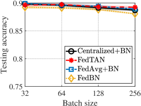
(a) i.i.d.

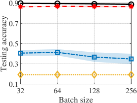
(b) Non-i.i.d.

Figure 12: FL Performance on CIFAR-10 dataset with different batch sizes. The mini-batch SGD without momentum or weight decay is adopted.

Appendix F Performance on DomainNet dataset

F.1 Dataset and DNN Model

In the experiments, we train AlexNet [15] on DomainNet dataset [42]. DomainNet dataset consists of natural images from six different data sources: clipart, infograph, painting, quickdraw, real, and sketch. It includes 345 classes of objects, and we conduct our experiments using the top ten most common classes, following the approach in the paper of FedBN [15]. We assume $N=6$ clients, and each client possesses training samples from one data source.

F.2 Parameter values

We adopt the identical parameter setting as described in [15], with a batch size of 32 and $\gamma$ set to 0.01, without applying momentum or weight decay.

F.3 Numerical Results

We label the FedBN schemes updated by clients with local datasets from clipart, infograph, painting, quickdraw, real, and sketch as FedBN-C, FedBN-I, FedBN-P, FedBN-Q, FedBN-R, and FedBN-S, respectively. The same notation applies to the SingleNet variants.

Fig. 13 presents a comparison of the performance of various FL schemes on testing datasets from different data sources and the whole global testing dataset. Similar to Fig. 8, FedBN outperforms SingleNet when the training and testing datasets come from different sources, thanks to its improved generalization ability. However, FedBN would still perform worse when datasets have different sources, such as FedBN-Q in Fig. 13(a)-13(c), 13(e), and 13(f), and FedBN-S in Fig. 13(a)-13(e). In contrast, FedTAN demonstrates superior generalization ability by aggregating model parameters in the server, leading to satisfactory performance across all testing datasets. Furthermore, FedTAN exhibits greater robustness compared to FedAvg+BN which is susceptible to gradient deviation.

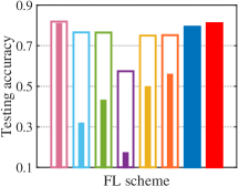
(a) Clipart.

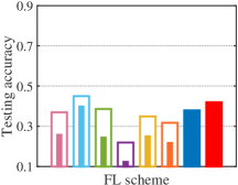
(b) Infograph.

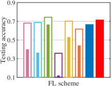
(c) Painting.

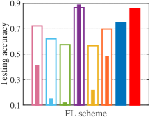
(d) Quickdraw.

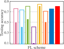
(e) Real.

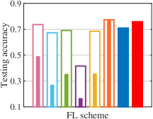
(f) Sketch.

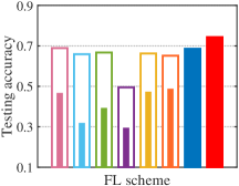
(g) Global.

Figure 13: Performance of different FL schemes on DomainNet dataset.

Appendix G Transmitted data volume of different FL schemes

G.1 FedAvg+GN

As ResNet-20 with GN contains 269722 parameters, the number of DNN parameters sent by the server to five clients and the number of parameters uploaded by five clients to the server are 269722 and 269722$\times$5, respectively. Hence, when using 32-bit (4-byte) floating point numbers to transmit DNN parameters, the total transmitted data volume between the server and clients per iteration in FedAvg+GN is $269722\times 6\times 4/1024/1024=6.1734$ MB.

G.2 FedAvg+BN

Using the same calculation process as before, and with 271098 parameters in ResNet-20 with BN, the total transmitted data volume in FedAvg+BN is $271098\times 6\times 4/1024/1024=6.2049$ MB per iteration.

G.3 FedTAN

ResNet-20 has 19 convolution layers, each followed by BN [14]. Then, with 16, 32, and 64 filters respectively in the first 7, middle 6, and last 6 convolution layers, respectively, the total number of statistical parameters (including batch mean and batch variance) in BN layers are $2\times(16\times 7+32\times 6+64\times 6)=1376$. As a result, during the layer-wise aggregations in Algorithm 2, the number of statistical parameters uploaded from five clients to the server and sent from the server to the clients is 1376$\times$5 and 1376, respectively. Therefore, for each iteration, the number of extra transmitted statistical parameters caused by Algorithm 2 is 1376$\times$6, and similarly, the number of extra transmitted gradients w.r.t. the statistical parameters caused by Algorithm 3 is 1376$\times$6 as well. Finally, the total amount of transmitted data between the server and clients per iteration in FedTAN, including the bits exchanged in the previous FedAvg+BN, is $(271098\times 6+1376\times 6+1376\times 6)\times 4/1024/1024=6.2679$ MB. $\blacksquare$

Appendix H Performance of FedTAN-II on MNIST Dataset

In this section, we demonstrate the effectiveness of FedTAN-II when applied to the MNIST dataset. Fig. 14(a) compares FedTAN-II with FedTAN by training a 3-layer DNN with BN on the MNIST dataset. The comparison is based on iterations. Furthermore, Fig. 14 (b) compares them in terms of communication rounds. For the FedTAN-II approach, we initialize the learning rate $\gamma$ at 0.5 for the first $M$ iterations, following the parameter setting of FedTAN in Section 6.1. Subsequently, the value of $\gamma$ is reduced to 0.05 after $M$ iterations.

As observed in Fig. 14, a reduction in the value of $M$ results in a marginal decrease in accuracy, especially if $M$ falls below a certain value (e.g., $M\leq 10$ in Fig. 14(a)). This slight accuracy reduction is primarily attributed to less precise statistical parameters. However, it is noteworthy that employing a smaller value for $M$ considerably diminishes the requisite communication rounds, as depicted in Figure 14(b).

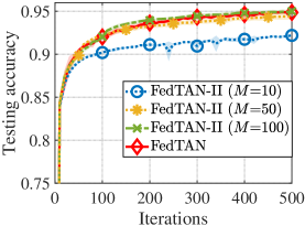
(a) Without momentum.

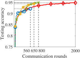
(b) Without momentum.

Figure 14: Testing accuracy of FedTAN-II on MNIST dataset.

Next, In Table 5, we contrast the aggregate exchanged bits, the proportions of supplementary communication rounds, and the exchanged bits resulting from layer-aggregations in Algorithms 2 and 3 throughout the complete training procedure of FedTAN-II across different $M$ values. As observed in Table 4, Table 5 further illustrates the insubstantial variance in total exchanged bits between FedTAN and FedTAN-II across varying $M$ values, owing to the minor proportion occupied by statistical parameters in BN layers within the total model size. Furthermore, while the additional communication rounds resulting from layer-aggregations in Algorithms 2 and 3 contribute to a specific proportion of the total exchanged bits throughout the training process, particularly evident with larger values of $M$, the accompanying extra exchanged bits remain negligible.

Table 5: Communication overhead of FedTAN-II on MNIST dataset.

FL scheme	Exchanged bits (GB)	Percentage of extra
		Rounds	Bits
FedTAN-II ($M$$=$10)	2.1388	5.66%	0.0100%
FedTAN-II ($M$$=$50)	2.1397	23.08%	0.0501%
FedTAN-II ($M$$=$100)	2.1408	37.50%	0.1002%
FedTAN	2.1386	75%	0.4992%

References

- [1] B. Luo, X. Li, S. Wang, J. Huang, and L. Tassiulas, “Cost-effective federated learning in mobile edge networks,” IEEE Journal on Selected Areas in Communications, vol. 39, no. 12, pp. 3606–3621, 2021.
- [2] Y. Wang, Y. Xu, Q. Shi, and T.-H. Chang, “Quantized federated learning under transmission delay and outage constraints,” IEEE Journal on Selected Areas in Communications, vol. 40, no. 1, pp. 323–341, 2022.
- [3] Y. Jiang, S. Wang, V. Valls, B. J. Ko, W.-H. Lee, K. K. Leung, and L. Tassiulas, “Model pruning enables efficient federated learning on edge devices,” IEEE Transactions on Neural Networks and Learning Systems, 2022.
- [4] T. Li, A. K. Sahu, M. Zaheer, M. Sanjabi, A. Talwalkar, and V. Smith, “Federated optimization in heterogeneous networks,” in Machine Learning and Systems (MLSys), vol. 2, 2020, pp. 429–450.
- [5] S. P. Karimireddy, S. Kale, M. Mohri, S. Reddi, S. Stich, and A. T. Suresh, “SCAFFOLD: Stochastic controlled averaging for federated learning,” in ICML, 2020, pp. 5132–5143.
- [6] B. Wei, J. Li, Y. Liu, and W. Wang, “Non-IID federated learning with sharper risk bound,” IEEE Transactions on Neural Networks and Learning Systems, 2022.
- [7] F. Sattler, S. Wiedemann, K.-R. Müller, and W. Samek, “Robust and communication-efficient federated learning from non-iid data,” IEEE transactions on neural networks and learning systems, vol. 31, no. 9, pp. 3400–3413, 2019.
- [8] J. Lu, C. Ni, and Z. Wang, “ETA: An efficient training accelerator for dnns based on hardware-algorithm co-optimization,” IEEE Transactions on Neural Networks and Learning Systems, 2022.
- [9] N. C. Thompson, S. Ge, and G. F. Manso, “The importance of (exponentially more) computing power,” arXiv preprint arXiv:2206.14007, 2022.
- [10] S. Zheng, C. Shen, and X. Chen, “Design and analysis of uplink and downlink communications for federated learning,” IEEE Journal on Selected Areas in Communications, vol. 39, no. 7, pp. 2150–2167, 2020.
- [11] Z. Chai, Y. Chen, L. Zhao, Y. Cheng, and H. Rangwala, “Fedat: A communication-efficient federated learning method with asynchronous tiers under non-iid data,” ArXivorg, 2020.
- [12] S. Santurkar, D. Tsipras, A. Ilyas, and A. Madry, “How does batch normalization help optimization?” Advances in neural information processing systems, vol. 31, 2018.
- [13] Y. Wu and K. He, “Group normalization,” in ECCV, 2018, pp. 3–19.
- [14] K. He, X. Zhang, S. Ren, and J. Sun, “Deep residual learning for image recognition,” in CVPR, 2016, pp. 770–778.
- [15] X. Li, M. Jiang, X. Zhang, M. Kamp, and Q. Dou, “FedBN: Federated learning on non-iid features via local batch normalization,” in ICLR, 2021.
- [16] K. Hsieh, A. Phanishayee, O. Mutlu, and P. Gibbons, “The non-iid data quagmire of decentralized machine learning,” in ICML, 2020, pp. 4387–4398.
- [17] Z. Du, J. Sun, A. Li, P.-Y. Chen, J. Zhang, H. Li, Y. Chen et al., “Rethinking normalization methods in federated learning,” arXiv:2210.03277, 2022.
- [18] M. Andreux, J. O. d. Terrail, C. Beguier, and E. W. Tramel, “Siloed federated learning for multi-centric histopathology datasets,” in Domain Adaptation and Representation Transfer, and Distributed and Collaborative Learning, 2020, pp. 129–139.
- [19] J. Mills, J. Hu, and G. Min, “Multi-task federated learning for personalised deep neural networks in edge computing,” IEEE Transactions on Parallel and Distributed Systems, vol. 33, no. 3, pp. 630–641, 2022.
- [20] M. J. Idrissi, I. Berrada, and G. Noubir, “FEDBS: Learning on non-iid data in federated learning using batch normalization,” in IEEE International Conference on Tools with Artificial Intelligence (ICTAI), 2021, pp. 861–867.
- [21] J.-H. Duan, W. Li, and S. Lu, “FedDNA: Federated learning with decoupled normalization-layer aggregation for non-iid data,” in Joint European Conference on Machine Learning and Knowledge Discovery in Databases, 2021, pp. 722–737.
- [22] R. Šajina, N. Tanković, and I. Ipšić, “Peer-to-peer deep learning with non-iid data,” Expert Systems with Applications, vol. 214, p. 119159, 2023.
- [23] E. Diao, J. Ding, and V. Tarokh, “HeteroFL: Computation and communication efficient federated learning for heterogeneous clients,” in ICLR, 2021.
- [24] B. McMahan, E. Moore, D. Ramage, S. Hampson, and B. A. y Arcas, “Communication-efficient learning of deep networks from decentralized data,” in Artificial Intelligence and Statistics, 2017, pp. 1273–1282.
- [25] S. Ioffe and C. Szegedy, “Batch normalization: Accelerating deep network training by reducing internal covariate shift,” in ICML, 2015, pp. 448–456.
- [26] X. Li, K. Huang, W. Yang, S. Wang, and Z. Zhang, “On the convergence of FedAvg on Non-IID data,” in ICLR, 2019.
- [27] A. Reisizadeh, A. Mokhtari, H. Hassani, A. Jadbabaie, and R. Pedarsani, “Fedpaq: A communication-efficient federated learning method with periodic averaging and quantization,” in International Conference on Artificial Intelligence and Statistics (AISTATS), 2020, pp. 2021–2031.
- [28] H. Yu, S. Yang, and S. Zhu, “Parallel restarted SGD with faster convergence and less communication: Demystifying why model averaging works for deep learning,” in AAAI, vol. 33, no. 01, 2019, pp. 5693–5700.
- [29] J. Wang, Q. Liu, H. Liang, G. Joshi, and H. V. Poor, “Tackling the objective inconsistency problem in heterogeneous federated optimization,” in NeurIPS, vol. 33, 2020, pp. 7611–7623.
- [30] L. Huang, D. Yang, B. Lang, and J. Deng, “Decorrelated batch normalization,” in CVPR, 2018, pp. 791–800.
- [31] X.-Y. Zhou, J. Sun, N. Ye, X. Lan, Q. Luo, B.-L. Lai, P. Esperanca, G.-Z. Yang, and Z. Li, “Batch group normalization,” arXiv:2012.02782, 2020.
- [32] X. Lian, C. Zhang, H. Zhang, C.-J. Hsieh, W. Zhang, and J. Liu, “Can decentralized algorithms outperform centralized algorithms? a case study for decentralized parallel stochastic gradient descent,” in NeurIPS, 2017, pp. 5336–5346.
- [33] Y. Wang, Q. Shi, and T.-H. Chang, “Why batch normalization damage federated learning on non-iid data?” arXiv:2301.02982, 2023.
- [34] Y. Huang, S. Gupta, Z. Song, K. Li, and S. Arora, “Evaluating gradient inversion attacks and defenses in federated learning,” in NeurIPS, vol. 34, 2021, pp. 7232–7241.
- [35] J. Zhong, H.-Y. Chen, and W.-L. Chao, “Making batch normalization great in federated deep learning,” arXiv preprint arXiv:2303.06530, 2023.
- [36] A. Krizhevsky et al., “Learning multiple layers of features from tiny images,” 2009.
- [37] Y. LeCun, L. Bottou, Y. Bengio, and P. Haffner, “Gradient-based learning applied to document recognition,” Proceedings of the IEEE, vol. 86, no. 11, pp. 2278–2324, 1998.
- [38] B. Gong, Y. Shi, F. Sha, and K. Grauman, “Geodesic flow kernel for unsupervised domain adaptation,” in CVPR. IEEE, 2012, pp. 2066–2073.
- [39] Y. Idelbayev, “Proper ResNet implementation for CIFAR10/CIFAR100 in PyTorch,” https://github.com/akamaster/pytorch_resnet_cifar10, 2021.
- [40] Weiaicunzai and Y. Kwon, “Practice on CIFAR-100 using PyTorch,” https://github.com/weiaicunzai/pytorch-cifar100, 2022.
- [41] L. Qu, Y. Zhou, P. P. Liang, Y. Xia, F. Wang, E. Adeli, L. Fei-Fei, and D. Rubin, “Rethinking architecture design for tackling data heterogeneity in federated learning,” in CVPR, 2022, pp. 10 061–10 071.
- [42] X. Peng, Q. Bai, X. Xia, Z. Huang, K. Saenko, and B. Wang, “Moment matching for multi-source domain adaptation,” in CVPR, 2019, pp. 1406–1415.
- [43] J. Zhang, D. Chen, J. Liao, W. Zhang, G. Hua, and N. Yu, “Passport-aware normalization for deep model protection,” NeurIPS, vol. 33, pp. 22 619–22 628, 2020.