Bayesian Graphical Entity Resolution using Exchangeable Random Partition Priors

Abstract

Entity resolution (record linkage or de-duplication) is the process of identifying and linking duplicate records in databases. In this paper, we propose a Bayesian graphical approach for entity resolution that links records to latent entities, where the prior representation on the linkage structure is exchangeable. First, we adopt a flexible and tractable set of priors for the linkage structure, which corresponds to a special class of random partition models. Second, we propose a more realistic distortion model for categorical/discrete record attributes, which corrects a logical inconsistency with the standard hit-miss model. Third, we incorporate hyperpriors to improve flexibility. Fourth, we employ a partially collapsed Gibbs sampler for inferential speedups. Using a selection of private and non-private data sets, we investigate the impact of our modeling contributions and compare our model with two alternative Bayesian models. In addition, we conduct a simulation study for household survey data, where we vary distortion, duplication rates and data set size. We find that our model performs more consistently than the alternatives across a variety of scenarios and typically achieves the highest entity resolution accuracy (F1 score). Open source software is available for our proposed methodology, and we provide a discussion regarding our work and future directions.

Statement of Significance

In survey statistics, entity resolution (record linkage) is used to identify responses submitted by the same individual across multiple surveys, even when unique identifiers such as social security numbers are not recorded. This paper advances Bayesian methods for entity resolution by: (i) thoroughly evaluating a general class of priors on links between responses and individuals, and (ii) proposing a more realistic model for distortions that appear in individuals’ identifying attributes (name, address, etc.). Both of these contributions are evaluated independently and jointly on a variety of data sets, one of which is a longitudinal medical survey. The results show that the general class of priors – the Ewens-Pitman random partitions – achieve similar accuracy in three previously studied parameter regimes, so long as vague hyperpriors are used. This is an important insight, as it addresses questions in the literature about which parameter regime (if any) is most suitable for entity resolution. In addition, the proposed distortion model is found to significantly improve the accuracy of entity resolution, particularly for string-type attributes. We provide two simulation studies supporting our work and comparisons. The paper is complemented by an R package that implements the proposed model using an optimized partially collapsed Gibbs sampler.

Keywords:  entity resolution, record linkage, Bayesian models, exchangeability, random partitions, Ewens-Pitman random partitions

1 Introduction

As commonly known in the literature, entity resolution (ER; record linkage or de-duplication) is the process of taking large, noisy (dirty) databases and removing duplicate records (often in the absence of a unique identifier) (Doan et al., 2012; Elmagarmid et al., 2007; Naumann and Herschel, 2010; Getoor and Machanavajjhala, 2012; Christen, 2012a; Christophides et al., 2020; Ilyas and Chu, 2019; Papadakis et al., 2021; Binette and Steorts, 2022). This problem has become increasingly important in many fields, such as survey methodology, official statistics, computer science, political science, health care, human rights, and others. In this paper, we are motivated by several applications. For example, we consider a longitudinal health care survey, where information is categorical in nature due to privacy restrictions on the data set. This may be of interest to those in the survey methodology community as they may face similar issues. In addition, we consider categorical and string or textual based data sets (or surveys) such as bibliographic/citation documents, information from restaurants, and a traditional benchmark (synthetic) study. The goal of analyzing multiple data sets is to make the survey community more aware of data sets that are relevant for entity resolution methods. Other overarching goals are to extend recent Bayesian graphical ER methodology for these data sets, provide comparative analyses, simulation studies, and guidance to researchers. Moreover, we provide open-source software for the community for our proposed method and two recently proposed methods in the literature.

The idea of entity resolution dates back to Dunn (1946), who envisioned a “book of life” that would piece together information about an individual. Newcombe et al. (1959) proposed one of the first methods for performing ER, based on a heuristic statistical test. This method was later formalized by Fellegi and Sunter (1969), who developed a model based on agreement patterns between pairs of records, and a likelihood ratio test for classifying pairs as linked (referring to the same entity), possibly linked or non-linked. Under some strong assumptions, they showed that their method – now known as the Fellegi-Sunter (FS) method – is statistically optimal. The FS method has been advanced over many decades in the ER literature, especially in survey methodology due to its scalability, ease of use and simplicity (Winkler, 2006; Christen, 2012a; Sadinle and Fienberg, 2013; Enamorado et al., 2019). However, it has some inherent limitations: it makes inconsistent (intransitive) predictions, it does not naturally account for uncertainty, it cannot exploit patterns at the entity-level, and it is incompatible with generative modeling approaches (Tancredi and Liseo, 2011).

Some of these limitations can be addressed by adapting the FS method to a Bayesian setting, while also imposing consistency constraints on the links between records (Sadinle, 2014, 2017). For example, Sadinle (2014) proposed a Bayesian extension of the FS model for performing ER within a single database. It incorporates consistency (transitivity) constraints by requiring that records are partitioned into groups that are mutually linked. In addition, the model supports multiple levels of agreement, and incorporates priors on the links and $m$/$u$ probabilities (from the FS model). In contrast with traditional FS methods, quantification of ER uncertainty is possible by computing the posterior distribution on the links. However, despite these benefits, the model has not been widely examined in the literature, perhaps in part due to the lack of a publicly-available implementation. One of our goals in this paper is to evaluate Sadinle’s model as a representative example of a Bayesian FS model, and compare it to another class of Bayesian entity resolution models, which we now describe.

In parallel to developments in Bayesian FS models, others have proposed a new class of generative models called Bayesian graphical entity resolution models (Tancredi and Liseo, 2011; Steorts, 2015; Steorts et al., 2016). In contrast with FS methods, these models do not operate on agreement patterns between pairs of records. Instead, they model a latent population of entities and the process by which records are generated from entities. They are known as “graphical” models because the fundamental objects in the model form a bipartite graph – the latent entities correspond to one set of vertices, the records correspond to another set of vertices, and the links are edges that connect the vertices. Tancredi and Liseo (2011) proposed one of the first models of this kind for performing ER across two databases. Subsequently, Steorts et al. (2016) proposed an extension to multiple databases, while optionally allowing for duplicates within each database. However, Steorts et al. (2016) discovered a limitation of the their model and the model by Tancredi and Liseo (2011) – the uniform prior on the linkage structure is highly informative about the number of entities present in the data. They noted that future work ought to consider more appropriate priors on the linkage structure for ER.

The models by Tancredi and Liseo (2011) and Steorts et al. (2016) both assume entities are described by a set of latent categorical attributes (e.g., date of birth, gender) which are distorted in the records. However, their model of the distortion process is simple and is unable to capture realistic distortions in string-type attributes, such as names. Steorts (2015) addressed this problem by proposing a string pseudo-likelihood and an empirically-motivated prior in a model known as blink. The blink model was later used as a foundation by Marchant et al. (2021) for developing more scalable Bayesian graphical ER techniques. They proposed an end-to-end method that jointly performs blocking and ER, where inference can be distributed or parallelized at the block level. Importantly, this enables propagation of blocking uncertainty to the ER task. They observed a 200$\times$ speed-up, which allowed them to scale blink to a data set containing over one million records. However, the blink model uses the same uniform prior on the linkage structure as Tancredi and Liseo (2011) and Steorts et al. (2016), and suffers from the same limitations.

Motivated by the shortcomings of existing Bayesian graphical ER models, we propose and evaluate several modeling refinements in this paper. First, we propose a flexible and tractable set of priors for the linkage structure that are the Ewens-Pitman (EP) family of random partition models (Pitman, 2006). These are the most general family of priors that satisfy exchangeability (an elementary requirement) and they are more flexible than the uniform priors used in previous work. Second, we incorporate hyperpriors on the EP parameters to further increase flexibility and reduce the need for tuning. This is motivated by the informativeness of the uniform prior used in previous work (Steorts et al., 2016). Third, we propose a more nuanced distortion model for categorical/discrete attributes, which corrects an inconsistency with the standard hit-miss model used by Tancredi and Liseo (2011); Steorts et al. (2016); Steorts (2015). Fourth, we design a partially collapsed Gibbs sampler to fit our model which incorporates computational optimizations.

We evaluate our modeling contributions independently and jointly on a selection of private and non-private data sets, and compare our model with the Bayesian graphical ER model by Steorts (2015) and the Bayesian FS model by Sadinle (2014). We also evaluate our model (and the alternatives) in a controlled simulation study, where we generate synthetic household survey data, with varying numbers of records, levels of distortion, and rates of duplication. Overall, we find our model is more robust across the various scenarios tested, and it typically achieves superior ER accuracies. We provide open source software for all of the ER methods under evaluation, and we provide a discussion of our contributions and directions for future work.

The rest of the paper proceeds as follows. Section 2 provides background on ER and exchangeable random partitions and outlines notation used throughout the paper. Section 3 outlines our proposed Bayesian graphical ER model. Section 4 presents a partially collapsed Gibbs sampling algorithm for approximating the posterior distribution and other computational speedups. Section 5 presents an empirical study of our proposed distortion model and linkage structure priors and includes a comparison to two recent Bayesian ER models. Section 5.5 summarizes a controlled simulation study that is in the Appendix. Section 6 summarizes our findings.

2 Background and Notation

In this section, we provide notation, assumptions, and a review of exchangeable random partitions which are used as a prior in our model. Figure 2 includes an index of symbols used throughout the paper.

2.1 Notation and Assumptions

We review notation and assumptions used throughout the paper. We assume the data (from one or more sources) is structured, meaning that it has been standardized using schema alignment techniques. For the purposes of our paper, the data is represented in a tabular format, where rows correspond to records and columns correspond to attributes. This in contrast to unstructured entity resolution, which deals with textual descriptions (paragraphs) or images. For a full review of these terms, see Papadakis et al. (2021).

Let $s\in\{1,\ldots,S\}$ be an index over the data sources and $i\in\{1,\ldots,N\}$ be an index over the records, which is unique across all sources. The source of the $i$-th record is denoted by $\varsigma_{i}\in\{1,\ldots,S\}$ and the record’s attribute values are represented as a tuple $\bm{x}_{i}=(x_{i1},\ldots,x_{iA})$ indexed by $a\in\{1,\ldots,A\}$. Assume $x_{ia}\in\mathcal{D}_{a}$ for all $i$ and $a$, where the domain of the $a$-th attribute $\mathcal{D}_{a}$ is a finite set of strings. Suppose there exists a (possibly infinite) population of entities indexed by $e\in\mathbb{N}$, which is represented in the data. Denote the entity referenced in the $i$-th record by $\lambda_{i}\in\mathbb{N}$ and define the linkage structure as $\bm{\Lambda}=(\lambda_{1},\ldots,\lambda_{N})$.

We consider the most general case where there are no constraints on $\bm{\Lambda}$ – i.e., we permit duplicates within sources and arbitrary links across sources. The linkage structure $\bm{\Lambda}$ induces a partition of the records into clusters. We label the clusters according to their associated entities, allowing for empty clusters. The size of cluster $e$ is denoted by $N_{e}=\sum_{i}\mathbb{1}[\lambda_{i}=e]$ and the number of non-empty clusters is denoted by $E=\sum_{e}\mathbb{1}[N_{e}>0]$.

We are interested in the fully unsupervised setting where no information is known about the linkage structure or the entities. Our goal is to infer the linkage structure based solely on the observed record attributes $\{\bm{x}_{1},\ldots,\bm{x}_{N}\}$ and source identifiers $\{\varsigma_{1},\ldots\varsigma_{N}\}$. Since we are working in a Bayesian setting, we seek a full posterior (not merely a point estimate) over the linkage structure so that uncertainty can be propagated to post-ER tasks, which may include regression, multiple systems estimation, among other examples (Kaplan et al., 2022; Tancredi and Liseo, 2015; Steorts et al., 2018; Tancredi et al., 2020; Sadinle, 2018). While the post-ER task is not a goal of this paper, the previous references propose recent approaches of such tasks.

2.2 Exchangeable Random Partitions

The linkage structure is the primary variable of interest for entity resolution, so we pay special attention to it when designing our model. Since we are working in a Bayesian setting, we must specify a prior on the linkage structure. We previously noted that the linkage structure can be interpreted as a partition of the records into subsets, where the records in each subset correspond to the same entity. This interpretation is convenient, as we can drawn on related work on random partitions when considering potential priors. In this section, we review a special class of random partitions called the Ewens-Pitman (EP) family (Pitman, 2006, p. 62), which we use as a prior on the linkage structure in our model (see Section 3).

Before defining the EP family of random partitions, we define key concepts and notation. Consider a set of $N$ records, where $[N]=\{1,\ldots,N\}$ denotes the record identifiers. A partition of $[N]$ is a collection of disjoint non-empty subsets of $[N]$. For example, $\{1,2\},\{3\}$ and $\{1\},\{2\},\{3\}$ are partitions of $[N]$ for $N=3$. We can equivalently define a partition in terms of the linkage structure $\bm{\Lambda}=(\lambda_{i})_{i=1\ldots N}$ where $\lambda_{i}$ labels the subset (entity) record $i$ is assigned to. Using this notation, the above examples for $N=3$ could be written as $\bm{\Lambda}=(1,1,2)$ and $\bm{\Lambda}=(1,2,3)$.

Let $\mathcal{P}_{[N]}$ denote the set of all partitions of $[N]$. A random partition of $[N]$ is a random variable whose values lie in $\mathcal{P}_{[N]}$. The EP family are the most general class of random partitions that satisfy the following two desirable properties:

1. Exchangeability. This means the distribution $P_{N}$ over the partitions $\mathcal{P}_{N}$ is invariant under permutations of the record identifiers $[N]$. Or equivalently, the distribution over $\bm{\Lambda}$ is exchangeable. This is a reasonable requirement if the records have no natural ordering – e.g., it is not known whether one record was generated before or after another.

2. Consistency. This is a property of the distribution as $N$ varies. It ensures the distribution is not altered when more records are observed. This is desirable because the model can be learned sequentially in a consistent manner. We say that the sequence of distributions $P_{1},P_{2},\ldots$ over $\mathcal{P}_{[1]},\mathcal{P}_{[2]},\ldots$ is consistent if the distribution on $\mathcal{P}_{[N]}$ induced by $P_{M}$ for $M>N$ is $P_{N}$. Mathematically, this means

   $$P_{M}(\{\rho:\mathsf{Proj}(\rho,[N])=\rho^{\prime}\})=P_{N}(\rho^{\prime}),$$

   where

   $$\mathsf{Proj}(\rho,[N]):=\{A_{e}\cap[N]:A_{e}\cap[N]\neq\emptyset,A_{e}\in\rho\}$$

   is the projection of a partition $\rho=\{A_{e}\}_{e=1\ldots E}$ of $[M]$ onto $[N]$ and $\rho^{\prime}$ is a partition of $[N]$.

In fact, the EP family ensures these properties hold in a limiting sense as $N\to\infty$ (Pitman, 2006, p. 62).

We can develop an intuitive understanding of the EP family by examining how a random partition is generated sequentially, one record at a time. Let $(\rho_{N})_{N=1,2,\ldots}$ be a sequence of EP random partitions where $\rho_{N}$ is a random partition of $[N]$. We begin at step 1 with $\rho_{1}=\{1\}$ – i.e., a single record assigned to a single entity. The random partition $\rho_{N}$ at any later step $N>1$ is generated conditional on the random partition $\rho_{N-1}$ at step $N-1$. Let $E$ be the number of subsets (occupied entities) in $\rho_{N-1}$ and $N_{e}$ be the size of subset (entity) $e$ in $\rho_{N-1}$. Then $\rho_{N}$ is generated by assigning record $N$ to:

• an existing subset (entity) with probability $\frac{N_{e}-\sigma}{N+\alpha}$, or

• a “new” subset (entity) with probability $\frac{\alpha+E\sigma}{N+\alpha}$,

where $\sigma$ and $\alpha$ are EP parameters. This construction is known as a two-parameter Chinese Restaurant Process and is visualized in Figure 1.

Figure 1: Illustration of a sequential construction of a Ewens-Pitman random partition. At step $N$ a record (black circle) is assigned to one of the occupied entities or a new entity (grey circles) conditioned on the assignments of the previous $N-1$ records. The probabilities assigned to the entities are given inside the grey circles and are dependent on the Ewens-Pitman parameters $\sigma$ and $\alpha$.

The allowable values of the EP parameters fall into two regimes depending on the sign of $\sigma$:

• $\sigma<0$ and $\alpha=-m\sigma$ for some $m\in\mathbb{N}$. We refer to this regime as the generalized coupon partitions, since they are closely related to the coupon-collector’s partition (Pitman, 2006, p. 46). These partitions are generated by sampling with replacement from a finite population of size $m$, where the mixing proportions are drawn from a symmetric Dirichlet distribution with concentration parameter $-\sigma$. The coupon-collector’s partition is obtained in the limit $\sigma\to-\infty$.

• $0\leq\sigma\leq 1$ with $\alpha>-\sigma$. These are called Pitman-Yor partitions after Pitman and Yor (1997), and are generated by sampling with replacement from an infinite population. The resulting partitions demonstrate preferential attachment behavior. The special case $\sigma=0$ corresponds to the Ewens partition (Kingman, 1978).

To illustrate the varying behavior of the random partitions as a function of $\sigma$, we can examine the asymptotic number of subsets in the partition (entities) $E_{N}$ as $N\to\infty$. Pitman (2006, p. 70) shows

$$E_{N}\overset{a.s.}{\asymp}\begin{cases}m,&\sigma<0\text{ and }\alpha=-m\sigma\text{ for }m\in\mathbb{N},\\ \alpha\log N,&\sigma=0\text{ and }\alpha>0,\\ S_{\sigma}N^{\sigma},&0<\sigma<1\text{ and }\alpha>-\sigma,\end{cases}$$ (1)

where $S_{\sigma}$ is a strictly positive random variable. Thus, by varying $\sigma$, we can encode a prior belief that the number of entities $E_{N}$ is asymptotically constant, logarithmic, or sub-linear in $N$.

3 Graphical Bayesian ER

In this section, we propose a generative model for entity resolution that incorporates a latent population of entities, each with a set of unknown attributes. Our model employs the Ewens-Pitman class of priors on the linkage structure and a modified record distortion model that deviates from the common “hit-miss” model used by Tancredi and Liseo (2011), Steorts (2015) and Steorts et al. (2016). We provide an index of the model’s variables and an illustration of their dependence structure in Figure 2. We close the section with a discussion of our model’s hyperparameters, including recommendations about how to set these values when limited prior information is available.

$i$	index over records
$s$	index over sources
$a$	index over attributes
$e$	index over entities
$x_{ia}$	attribute $a$ for record $i$
$z_{ia}$	distortion indicator for attribute $a$ of record $i$
$\omega_{ia}$	distortion propensity for attribute $a$ of record $i$
$\varsigma_{i}$	source of record $i$
$\lambda_{i}$	linked entity for record $i$

$H_{ea}$	distortion distribution for attribute $a$ of entity $e$
$\rho_{a}$	concentration of $H_{ea}$
$\bm{\psi}_{a}$	base distribution for $H_{ea}$
$\theta_{sa}$	distortion probability for attribute $a$ in source $s$
$y_{ea}$	attribute $a$ for entity $e$
$G_{a}$	distribution over domain for attribute $a$
$\bm{\pi}$	mixing proportions
$\sigma$, $\alpha$	Ewens-Pitman parameters
$\mathcal{D}_{a}$	domain of attribute $a$
$\operatorname{dist}_{a}$	distance measure for attribute $a$

Figure 2: Plate diagram and index of symbols for our model under a Pitman-Yor prior.

3.1 Model Specification

Entities.

We assume each entity $e\in\{1,2,\ldots\}$ is associated with a tuple of attribute values $\bm{y}_{e}=(y_{e1},\ldots,y_{eA})$, drawn independent and identically distributed (i.i.d.) from an unknown distribution $\bm{G}$ with support on $\mathcal{D}=\prod_{a}\mathcal{D}_{a}$. To improve tractability, we assume correlations between attributes are negligible, and place independent Dirichlet Process (DP) priors on each component of $\bm{G}=(G_{1},\ldots,G_{A})$:

$$G_{a} \overset{\mathrm{ind.}}{\sim}\operatorname{DP}\!\left(\upsilon_{a},\phi_{a}\right), \forall a,$$

$$y_{ea}\mid G_{a} \overset{\mathrm{ind.}}{\sim}\operatorname{Discrete}(G_{a}), \forall e,a,$$

where $\upsilon_{a}>0$ is a concentration parameter and $\phi_{a}$ is a base distribution on domain $\mathcal{D}_{a}$.

Links.

Each record $i\in\{1,\ldots,N\}$ is linked to an entity $\lambda_{i}\in\{1,2,\ldots\}$ which is assumed to be drawn from the population with replacement, according to unknown mixing proportions $\bm{\pi}=(\pi_{1},\pi_{2},\ldots)$. This process induces a partition of the records into clusters according to their linked entities. Following the discussion about exchangeability in Section 2.2, we assume the partition is drawn from the Ewens-Pitman (EP) family with parameters $(\sigma,\alpha)$. The corresponding distribution on the mixing proportions $\bm{\pi}$ depends on the sign of $\sigma$, or equivalently, whether the population of entities is finite or infinite.

For the finite regime (generalized coupon partitions) we let $\sigma=-\kappa<0$ and $\alpha=m\kappa$ for some $m\in\mathbb{N}$. Our model with hyperpriors on $m$ and $\kappa$ is as follows:

$$\kappa \sim\operatorname{Gamma}(\chi^{(0)},\chi^{(1)}),$$ (2)

$$m \sim\operatorname{NegativeBinomial}(r,\nu)+1,$$

$$\bm{\pi}\mid\kappa,m \sim\operatorname{Dirichlet}(\bm{\kappa}),$$

$$\lambda_{i}\mid\bm{\pi} \overset{\mathrm{iid.}}{\sim}\operatorname{Categorical}(\bm{\pi}), \forall i,$$

where $\chi^{(0)},\chi^{(1)},r>0$ and $0<\nu\leq 1$ are hyperparameters, and $\bm{\kappa}$ is a vector of length $m$ with identical entries $\kappa$. The hyperprior on $m$ is a shifted negative binomial distribution with density defined in Appendix A.4.2.

In the infinite regime (Pitman-Yor partitions) the mixing proportions are drawn from a two-parameter Poisson-Dirichlet distribution (Pitman and Yor, 1997). Our model with hyperpriors on $\sigma$ and $\alpha$ is as follows:

$$\sigma \sim\operatorname{Beta}(\zeta^{(0)},\zeta^{(1)}),$$ (3)

$$\alpha \sim\operatorname{Gamma}(\chi^{(0)},\chi^{(1)}),$$

$$\bm{\pi}\mid\sigma,\alpha \sim\operatorname{PoissonDirichlet}(\sigma,\alpha),$$

$$\lambda_{i}\mid\bm{\pi} \overset{\mathrm{iid.}}{\sim}\operatorname{Categorical}(\bm{\pi}), \forall i,$$

where $\chi^{(0)},\chi^{(1)},\zeta^{(0)},\zeta^{(1)}>0$ are hyperparameters. Here we assume $\alpha>0$ and $0<\sigma<1$, which is a subset of the admissible parameter space: $0\leq\sigma\leq 1$ and $\alpha>-\sigma$. We also consider the case where $\sigma=0$, which corresponds to the Ewens partition.

Remark.

By placing hyperpriors on the EP parameters, we can improve robustness to misspecified hyperparameters which are difficult to set in a non-informative manner. Special cases of the above priors have been used in other ER models, albeit with fixed hyperparameters. Tancredi and Liseo (2011), Steorts (2015) and Steorts et al. (2016) used a coupon-collector’s partition with $\kappa\to\infty$ and $m$ fixed, which was shown to be highly informative for the observed population size. Steorts et al. (2018) used a Pitman-Yor partition with $\sigma$ and $\alpha$ fixed.

Sources.

We assume the data source $\varsigma_{i}\in\{1,\ldots,S\}$ associated with record $i$ is drawn i.i.d. from a discrete distribution $\bm{\xi}$ over the sources $\{1,\ldots,S\}$. There is no need to specify $\bm{\xi}$ since it is independent of the other model parameters, and the source indicators $\varsigma_{i}$ are assumed to be fully observed.

Distortion.

We assume the attributes $\bm{x}_{i}$ for record $i$ are generated by distorting the associated entity attributes $\bm{y}_{\lambda_{i}}$. For simplicity, we assume the distortion process occurs independently for each attribute. To decide whether the $a$-th attribute is distorted, a binary indicator $z_{ia}$ is drawn which depends on the distortion propensity $\omega_{ia}$ scaled by a source/attribute-level factor $\theta_{\varsigma_{i}a}$. We place a Beta prior on $\theta_{\varsigma_{i}a}$ and assume the distortion propensity $\omega_{ia}$ is deterministic given the true attribute value $y_{\lambda_{i}a}$. Concretely, we have

$$\theta_{sa} \overset{\mathrm{ind.}}{\sim}\operatorname{Beta}\!\left(\beta_{sa}^{(0)},\beta_{sa}^{(1)}\right) \forall s,a$$ (4)

$$\omega_{ia}\mid y_{\lambda_{i}a} =\mathrm{propensity}\left(\min_{x\in\mathcal{D}_{a}\setminus\{y_{\lambda_{i}a}\}}\operatorname{dist}_{a}(y_{\lambda_{i}a},x),\max_{x,y\in\mathcal{D}_{a}}\operatorname{dist}_{a}(y,x)\right) \forall i,a$$

$$z_{ia}\mid\theta_{\varsigma_{i}a},\omega_{ia} \overset{\mathrm{ind.}}{\sim}\operatorname{Bernoulli}\!\left(\theta_{\varsigma_{i}a}\omega_{ia}\right) \forall i,a$$ (5)

where $\beta_{sa}^{(0)},\beta_{sa}^{(0)}>0$ are hyperparameters and

$$\mathrm{propensity}(d_{\mathrm{min}},d_{\mathrm{max}}):=\begin{cases}0,&d_{\mathrm{min}}=\infty\text{ and }d_{\mathrm{max}}=\infty,\\ 1,&d_{\mathrm{min}}=0\text{ and }d_{\mathrm{max}}=0,\\ \mathrm{e}^{-\frac{d_{\mathrm{min}}}{2d_{\mathrm{max}}}},&\text{otherwise.}\end{cases}$$ (6)

The distortion propensity $\omega_{ia}$ accounts for the fact that some entity attribute values $y_{\lambda_{i}a}\in\mathcal{D}_{a}$ are more likely to be distorted than others. It makes use of prior information in the attribute distance measure $\operatorname{dist}_{a}(y,x)$ (see Section 3.2). If $y_{\lambda_{i}a}$ is not close to any other values in the domain, it is unlikely to be distorted and $\omega_{ia}$ approaches zero. On the other hand, if $y_{\lambda_{i}a}$ is close to at least one other value in the domain, distortion can occur and $\omega_{ia}$ approaches one. This logic is not included in a similar model by Steorts (2015), which effectively assumes $\omega_{ia}=1$.

After drawing the distortion indicator $z_{ia}$, record attribute $x_{ia}$ is generated by copying the linked entity attribute $y_{\lambda_{i}a}$ directly (if $z_{ia}=0$) or subject to distortion (if $z_{ia}=1$). If $z_{ia}=1$, the distorted value is drawn from a distortion distribution $H_{\lambda_{i}a}$ associated with the linked entity $\lambda_{i}$. We assume $H_{\lambda_{i}a}$ itself is drawn from a Dirichlet Process:

$$\rho_{a} \sim\operatorname{Gamma}\!\left(\tau_{a}^{(0)},\tau_{a}^{(1)}\right) \forall a,$$ (7)

$$H_{ea}\mid y_{ea},\rho_{a} \overset{\mathrm{ind.}}{\sim}\operatorname{DP}\!\left(\rho_{a};\bm{\psi}_{a}(y_{ea})\right) \forall e,a,$$ (8)

where $\tau_{a}^{(0)},\tau_{a}^{(1)}>0$ are hyperparameters, and $\bm{\psi}_{a}(y_{ea})$ is a prior base distribution with support on a subset of $\mathcal{D}_{a}\setminus\{y_{\lambda_{i}a}\}$. This differs from models by Tancredi and Liseo (2011), Steorts (2015) and Steorts et al. (2016, 2018), which assume $H_{ea}$ is deterministic conditional on $y_{ea}$.

Summarizing this symbolically, we have

$$x_{ia}\mid z_{ia},y_{\lambda_{i}a},H_{\lambda_{i}a} \overset{\mathrm{ind.}}{\sim}\begin{cases}\delta(y_{\lambda_{i}a}),&\text{if }z_{ia}=0,\\ H_{\lambda_{i}a},&\text{if }z_{ia}=1,\end{cases} \forall i,a$$ (9)

where $\delta(y)$ denotes a point mass at $y$. This is reminiscent of a hit-miss model (Copas and Hilton, 1990). However, our construction differs, in that the record and entity attributes are forbidden from matching ($x_{ia}\neq y_{\lambda_{i}a}$) if the record attribute is distorted ($z_{ia}=1$).

Remark.

The hit-miss model of Copas and Hilton (1990) was designed for modeling distortion of continuous attributes. For continuous attributes, the probability of drawing the non-distorted value ($y_{\lambda_{i}a}$) from the miss component $H_{\lambda_{i}a}$ is zero, assuming $H_{\lambda_{i}a}$ is described by a continuous density function. This ensures the record value $x_{ia}$ is always distorted ($x_{ia}\neq y_{\lambda_{i}a}$) if $z_{ia}=1$. Our proposal replicates the same behavior for discrete attributes by ensuring $H_{ea}$ has no mass on $y_{ea}$. This is especially important if $H_{ea}$ were to place significant mass on $y_{ea}$, as the line between distorted and non-distorted values would become blurred. Apart from the modeling advantages, excluding $y_{ea}$ from the support of $H_{ea}$ also makes inference more tractable as we can collapse $H_{ea}$ (see Appendices A.2 and A.3).

3.2 Choice of Hyperparameters

In this section, we provide recommendations for setting the hyperparameters in our model.

Distance Measures.

Our proposed distortion model is parameterized by a set of distance measures $\{\operatorname{dist}_{a}\}$, one for each attribute $a\in\{1,\ldots,A\}$. They encode prior knowledge about the likelihood that a record attribute value $x$ appears as a distorted alternative to an entity attribute value $y$. The larger the distance $\operatorname{dist}_{a}(y,x)$, the less likely $x$ is a distortion of $y$. Since the likelihood of distorting $x$ to $y$ may not be the same as the likelihood of distorting $y$ to $x$, we do not require that the distance measures are symmetric. We recommend selecting the distance measures carefully, leveraging prior knowledge about the distortion process where possible. For instance, one might select edit distance to model typographic distortion in a generic string-type attribute. For categorical attributes, one could select a constant distance function $\operatorname{dist}_{a}(y,x)\equiv 0$, which encodes the prior belief that all values in the domain are equally likely as a distorted alternative to $y$.

Distortion Base Distribution.

We recommend using the distance measures to set the base distribution $\bm{\psi}_{a}(y_{ea})$ in Equation (8). Specifically, we recommend a softmax distribution

$$\psi_{a}(x\mid y_{ea})\propto\mathbb{1}[x\neq y_{ea}]\exp(-\operatorname{dist}_{a}(y_{ea},x)),$$ (10)

where the temperature parameter is absorbed in the definition of the distance measure, and the indicator function excludes $y_{ea}$ from the support. This places more weight on values in the domain closer to $y_{ea}$ and less weight on values further away. Unlike Steorts (2015), we do not include a factor proportional to the empirical frequency of $x$, as distorted values (e.g., typographical errors) tend to be infrequent for the applications we consider. For a categorical attribute with $\operatorname{dist}_{a}(y,x)\equiv 0$, Equation (10) reduces to the uniform distribution. In this case, it may be appropriate to incorporate a factor proportional to the empirical frequencies by setting $\psi_{a}(x\mid y_{ea})\propto\mathbb{1}[x\neq y_{ea}]\sum_{i=1}^{N}\mathbb{1}[x_{ia}=x]$.

Other Hyperparameters.

In the absence of prior knowledge, we recommend setting the remaining hyperparameters to yield vague priors – i.e., priors that provide little information relative to the experiment (Tiao and Box, 1973; Bernardo and Smith, 2009). We note that there are different views in the Bayesian community about how to specify vague and/or uninformative priors. For more on this, we refer to Syversveen (1998) and Irony and Singpurwalla (1997). Putting aside such debates, our recommendations are as follows:

• For the shifted negative binomial prior on $m$, we set $r$ and $\nu$ so that the prior mean is $N$ and the prior variance is $N^{2}$.

• For the gamma prior on $\alpha$, we set $\chi^{(0)}=1$ and $\chi^{(1)}$ to be small (e.g., $10^{-2}$).

• For the beta prior on $\sigma$, we set $\zeta^{(0)}=\zeta^{(1)}=1$ to yield a flat prior.

• For the Dirichlet prior on the entity attribute distribution, we recommend setting $\upsilon_{a}=1$ and using a uniform base distribution $\phi_{a}$ for all $a$.

• For the gamma prior on the concentration parameter $\rho_{a}$, we recommend setting $\tau^{(0)}=2$ and $\tau^{(1)}$ small (e.g., $10^{-4}$) for all $a$.

• For the beta priors on $\theta_{s,a}$, we encode a weak prior belief of low distortion by setting $\beta_{sa}^{(0)}=1$ and $\beta_{sa}^{(1)}=4$ for all $s,a$.

Remark.

The hyperparameters can be varied to encourage over-linkage (linking records that do not correspond to the same entity) or under-linkage (failing to link records that correspond to the same entity). Since perfect linkage is not always possible, practitioners may have to decide whether over-linkage or under-linkage is preferred for a given application. We can encourage over-linkage in our model by setting:

• $\beta_{sa}^{(0)}\gg\beta_{sa}^{(1)}$ (prior belief of high distortion),

• $\upsilon_{a}\ll 1$ (prior belief of low diversity in attribute $a$ among entities),

• $\zeta^{(0)}\ll\zeta^{(1)}$ and $\chi^{(0)}\ll\chi^{(1)}$ (prior belief of more links for Pitman-Yor prior), or

• $r$ close to 0 and $\nu$ close to 1 (prior belief of more links for generalized coupon prior).

Similarly, we can encourage under-linkage by reversing the inequalities above. We measure the extent to which our model over- or under-links in our empirical evaluation (Section 5) using precision and recall metrics defined in Equations (12) and (13).

4 Inference

To perform entity resolution using our model, we must find the posterior distribution over the linkage structure conditional on the observed record attributes and their sources. Since the posterior is not analytically tractable, we propose an approximate inference scheme based on Markov chain Monte Carlo (MCMC).

MCMC produces approximate samples from the posterior distribution by constructing a Markov chain whose equilibrium distribution matches the posterior distribution. The samples produced by MCMC are approximate in the sense that they are autocorrelated, and they may only match the equilibrium (posterior) distribution asymptotically. Various algorithms exist within the MCMC framework – we refer the reader to Gamerman and Lopes (2006) or Brooks et al. (2011) for an introduction to the field.

In this paper, we use an MCMC algorithm called partially collapsed Gibbs (PCG) sampling (van Dyk and Park, 2008). It is a generalization of Gibbs sampling that reduces the extent of conditioning in the variable updates by collapsing (marginalizing out) variables and/or updating variables in groups. This can significantly improve convergence and reduce autocorrelation, so long as prescribed rules are followed to ensure the equilibrium distribution of the Markov chain is preserved.

Ideally, we would like to reduce the extent of conditioning as much as possible, however this must be balanced with computational and mathematical constraints. In our proposed sampling scheme, we fully collapse the entity mixing proportions $\bm{\pi}$ and the distortion distributions $H_{ea}$. We partially-collapse the distortion indicators $z_{ia}$ in a joint update for the entity attributes $y_{ea}$ and for the distortion distribution concentration $\rho_{a}$. By collapsing the mixing proportions, we obtain an urn-based scheme for updating the linkage structure similar to those used for nonparametric mixture models (Neal, 2000). In the remainder of this section, we highlight some less trivial aspects of inference – full details are provided in Appendix A.

4.1 Nonconjugacy

While we attempted to maintain conjugacy in our model, we were unable to avoid nonconjugate priors in some cases. This complicates inference, as the posterior conditional distributions used in Gibbs sampling are no longer of a standard form. There are several well-established methods for dealing with nonconjugacy, including Metropolis-Hastings algorithms (Chib and Greenberg, 1995), rejection sampling (Gilks and Wild, 1992) and auxiliary variable methods (Damlen et al., 1999). We opt to use auxiliary variable methods owing to their simplicity, as there is no need to design proposals or monitor acceptance rates.

There are three sets of parameters in our model for which nonconjugacy is an issue:

1. The distortion probabilities $\theta_{sa}$ defined in Equation (4), where the incorporation of the distortion propensities $\omega_{ia}$ breaks the conjugacy of the beta prior. We propose an auxiliary variable sampling scheme to update $\theta_{sa}$ in Appendix A.1.

2. The EP parameters: $\kappa$ and $m$ defined in Equation (2) or $\alpha$ and $\sigma$ defined in Equation (3), depending on the regime. We use an auxiliary variable scheme proposed by Teh (2006), to update $\alpha$ and $\sigma$ under a gamma and beta prior, as summarized in Appendix A.4.1. We design an auxiliary variable update for $\kappa$ and $m$ under a gamma and shifted negative binomial prior in Appendix A.4.2.

3. The distortion distribution concentration $\rho_{a}$ defined in Equation (7). We design an auxiliary variable update for $\rho_{a}$ in Appendix A.5.

4.2 Collapsing the Distortion Indicators

Marchant et al. (2021) demonstrated the importance of collapsing the distortion indicators $\{z_{ia}\}$ to improve convergence/mixing for a hit-miss model similar to Equation (9). The posterior factors involving $z_{ia}$ factorize over $i$ and $a$, so that collapsing $z_{ia}$ yields:

$$P(x_{ia}\mid\theta_{\varsigma_{i}a},\omega_{ia},y_{\lambda_{i}a},H_{\lambda_{i}a}) \propto\sum_{z_{ia}=0}^{1}P(x_{ia}\mid z_{ia},y_{\lambda_{i}a},H_{\lambda_{i}a})P(z_{ia}\mid\theta_{\varsigma_{i}a},\omega_{ia})$$

$$\propto(1-\theta_{\varsigma_{i}a}\omega_{ia})\mathbb{1}[x_{ia}=y_{\lambda_{i}a}]+\theta_{\varsigma_{i}a}\omega_{ia}H_{\lambda_{i}a}(x_{ia}).$$ (11)

We use this result to implement a collapsed update for the entity attributes $\{y_{ea}\}$. While it is possible to implement a collapsed update for the linkage structure $\{\lambda_{i}\}$, we opt not to do so, since conditioning on the distortion indicators allows us to reduce computational complexity via indexing (see Section 4.3). This seems to be more efficient empirically (Marchant et al., 2021), so long as the level of distortion is not too high.

4.3 Computational Considerations

We now discuss ways of improving the computational complexity. The main bottleneck is the update for the linkage structure which scales naïvely as $O(N\cdot E)$ where $E$ is the number of instantiated entities. The update for the entity attributes may also be problematic for large domains $\mathcal{D}_{a}$ as it scales as $O(E\cdot\lvert\mathcal{D}_{a}\rvert)$ for the $a$-th attribute.

We are able to reduce the computational complexity of the linkage structure update by exploiting constraints imposed by the distortion model. Close inspection of the update for the entity linked to record $i$ (see Appendix A.3) reveals that some entities can be immediately excluded from consideration. Specifically, only those entities whose attributes match the corresponding non-distorted record attributes ($x_{ia}$ with $z_{ia}=0$) may be linked to record $i$. In order to efficiently query this set of entities, we maintain inverted indices that map an attribute value $x\in\mathcal{D}_{a}$ to the set of entities instantiated with that value $\{e:x=y_{ea}\}$. This approach is considerably more efficient than iterating over all entities sequentially, so long as the level of distortion is relatively low. However it is important to note that it relies crucially on not collapsing the distortion indicators.

To improve the complexity of the entity attribute update, we can impose a cut-off on the distance measures. Concretely, for attribute $a$ we replace the “raw” distance measure $\operatorname{dist}_{a}$ by

$$\underline{\operatorname{dist}}_{a}(y,x)=\begin{cases}\operatorname{dist}_{a}(y,x),&\text{if }\operatorname{dist}_{a}(y,x)\leq d_{a}^{(\mathrm{cut})},\\ \infty,&\text{otherwise},\end{cases}$$

where $d_{a}^{(\mathrm{cut})}\in(0,\infty)$ is a configurable cut-off. This approximation eliminates the need to consider unlikely distortions from entity attribute $y$ to record attribute $x$, for which $\operatorname{dist}(y,x)>d_{a}^{(\mathrm{cut})}$. It plays a similar role to blocking in the record linkage literature (Christen, 2012b) and resembles an approach proposed by Marchant et al. (2021). To make use of this approximation, we build indices that can efficiently answer range queries – one for each attribute. The index for the $a$-th attribute takes a query value $x\in\mathcal{D}_{a}$ and returns the set of entity attribute values that fall below the cut-off: $\{y\in\mathcal{D}_{a}:\operatorname{dist}_{a}(y,x)\leq d_{a}^{(\mathrm{cut})}\}$.

5 Model Comparisons

We conduct an empirical study of our ER model using data sets for which the true linkage structure is known. Section 5.1 describes the data sets used in the study, which are motivated by ER applications in private and non-private settings. We explain how our model (and baseline models) are evaluated in Section 5.2, by computing metrics that assess how well the posterior predictions align with the true linkage structure. Section 5.3 assesses the impact of our modeling contributions by varying the distortion model and the prior on the linkage structure. Section 5.4 compares our ER model against baselines proposed by Sadinle (2014) and Steorts (2015). Finally, Section 5.5 summarizes a controlled simulation study that can be found in Appendix C.

5.1 Data Sets

We study entity resolution in private and non-private settings, both of which are encountered by practitioners. The data sets we use in our study are summarized in Table 1.

Private Setting.

In this setting the practitioner has access to de-identified data, where sensitive attributes such as names, addresses, phone numbers, etc. are removed. This can make ER quite challenging, as the remaining non-sensitive attributes may carry limited information about the identity of records. To study ER in this setting, we use data extracted from the National Long Term Care Survey (Manton, 2010), which we refer to as nltcs.

Our extract contains de-identified respondent records from the 1982, 1989 and 1994 waves of the survey in the U.S. state of Alabama. We use all of the available attributes for ER, which include date of birth (DOB_YEAR, DOB_MONTH, DOB_DAY), registration office (REGOFF) and sex (SEX). Since the data is well-curated, the only distortion that can occur is when a valid attribute value is replaced by another valid attribute value. We, therefore, model the attributes as categorical by employing a constant distance function.

Non-private Setting.

In this setting, the practitioner has access to data with sensitive attributes, such as names. We assume unique identifiers such as social security numbers are not available, as ER would otherwise be trivial. Obtaining real survey data for a non-private setting with ground truth is challenging, so we use three publicly-available data sets from the ER literature. Although these data sets cover other domains, they exhibit characteristics one would expect to encounter in real survey data. Namely, we observe the presence of multiple “name-like” attributes, as well as different levels of variation and distortion. Below, we provide a brief description of each data set and the attributes used for ER:

• RLdata is a synthetic person data set, where 10% of the records are duplicates with random errors (Sariyar and Borg, 2010). We model the name attributes (fname_c1 and lname_c1) using the normalized Levenshtein distance measure. The attributes related to date of birth – bd, bm and by – are modeled as categorical attributes with a constant distance measure.

• cora is a collection of computer science citation records hosted on the RIDDLE repository (Bilenko, 2003). It is the “dirtiest” of all the data sets we consider, as it was extracted from various online sources with different citation styles. As a pre-processing step, we separate hyphenated words and remove punctuation. We also correct several erroneous ground truth labels. The title, venue and authors attributes generally contain multiple words with semantic and character-level variations, and are therefore modeled using a hybrid token/edit distance measure described in Appendix B. The year attribute is modeled using normalized Levenshtein distance.

• rest is a collection of restaurant records from the Fodor and Zagat restaurant guides hosted on the RIDDLE repository (Bilenko, 2003). It is not as “dirty” as cora as there are fewer sources and less variation between them. We applied the same pre-processing steps as for cora. The name and addr attributes generally contain multiple words and are therefore modeled using the same hybrid distance measure as for cora. The city and type (cuisine) attributes are modeled as categorical with a constant distance measure.

Data set	Setting	Entity type	# records ($N$)	# entities
nltcs	Private	People	5,359	3,307
RLdata	Non-private	People	10,000	9,000
cora	Non-private	Citations	1,295	125
rest	Non-private	Restaurants	864	752

Table 1: Summary of data sets.

5.2 Model Evaluation

We evaluate an ER model on a data set by comparing the inferred linkage structure $\hat{\Lambda}$ to the true linkage structure $\Lambda$. Recall that $\Lambda=(\lambda_{1},\ldots,\lambda_{N})$ specifies the corresponding entity $\lambda_{i}$ for each record $i$ in the data set. The agreement between $\hat{\Lambda}$ and $\Lambda$ can be measured using pairwise precision and recall. The pairwise precision is the proportion of record pairs linked in $\hat{\Lambda}$ that are also linked in $\Lambda$:

$$\operatorname{Pr}(\hat{\Lambda},\Lambda)=\frac{\sum_{i\neq j=1}^{N}\mathbb{1}[\hat{\lambda}_{i}=\hat{\lambda}_{j}]\mathbb{1}[\lambda_{i}=\lambda_{j}]}{\sum_{i\neq j=1}^{N}\mathbb{1}[\hat{\lambda}_{i}=\hat{\lambda}_{j}]}.$$ (12)

It takes on values from 0 to 1, where larger values indicate fewer false positive errors. The pairwise recall is the proportion of record pairs linked in $\Lambda$ that are also linked in $\hat{\Lambda}$:

$$\operatorname{Re}(\hat{\Lambda},\Lambda)=\frac{\sum_{i\neq j=1}^{N}\mathbb{1}[\hat{\lambda}_{i}=\hat{\lambda}_{j}]\mathbb{1}[\lambda_{i}=\lambda_{j}]}{\sum_{i\neq j=1}^{N}\mathbb{1}[\lambda_{i}=\lambda_{j}]}.$$ (13)

It takes on values from 0 to 1, where larger values indicate fewer false negative errors. It is rarely possible to achieve high precision and recall – one must usually make a trade-off depending on which types of errors are more costly in a given application. If precision and recall are equally important, then one can measure the agreement between $\hat{\Lambda}$ and $\Lambda$ using the pairwise F1 score which is the harmonic mean of precision and recall:

$$\operatorname{F1}(\hat{\Lambda},\Lambda)=2\frac{\operatorname{Pr}(\hat{\Lambda},\Lambda)\cdot\operatorname{Re}(\hat{\Lambda},\Lambda)}{\operatorname{Pr}(\hat{\Lambda},\Lambda)+\operatorname{Re}(\hat{\Lambda},\Lambda)}.$$ (14)

Since the models in our study are Bayesian, the inferred (posterior) linkage structure $\hat{\Lambda}$ is a random variable and the metrics in Equations (12)–(14) can be regarded as random variables. We estimate the distribution of the metrics under the posterior using samples generated via MCMC. In doing so, we are able to account for posterior uncertainty in our evaluation. For each metric, we report a point estimate using the median, along with a 95% equi-tailed credible interval. Further details about the MCMC implementation and configuration for each model are provided in Appendix E and MCMC diagnostics are in Appendix G.

5.3 Study of Linkage Structure Priors and Distortion Model

In this section, we study the effect of two modeling contributions proposed in Section 3.1 – the Ewens-Pitman (EP) linkage structure priors and the refined distortion model. Our objective is to determine the impact of each modeling contribution in isolation, using the blink model as a baseline. We summarize the results here and refer the reader to Appendix D for comprehensive results covering eight combinations of linkage structure priors and distortion models.

Linkage Structure Priors.

We consider four priors on the linkage structure, which correspond to distinct EP parameter regimes (see Section 2.2):

1. PY: Pitman-Yor regime with $\sigma\in(0,1)$ and hyperpriors on $\sigma,\alpha$ as detailed in Equation (3).

2. Ewens: Ewens regime with $\sigma=0$ and a hyperprior on $\alpha$ as detailed in Equation (3).

3. GenCoupon: generalized coupon regime with $\sigma=-\kappa<0$ and hyperpriors on $\kappa,m$ as detailed in Equation (2).

4. Coupon: coupon collector’s partition used by with $\kappa\to\infty$ and $m=N$.

The first three priors are flexible, in the sense that hyperpriors are placed on the EP parameters. The last prior is a particular instance of GenCoupon where the EP parameters are fixed. It is used in models by Tancredi and Liseo (2011), Steorts (2015) and Steorts et al. (2016), and serves as a baseline here.

ER evaluation metrics are presented in Table 2 for the four linkage structure priors, assuming the rest of the model follows the specification in Section 3.1. Another perspective on ER accuracy is provided in Figure 3, which plots the relative error in the inferred number of entities. Both results demonstrate the benefit of placing hyperpriors on the EP parameters, as is done for PY, Ewens, and GenCoupon. These linkage structure priors achieve superior F1 scores compared to Coupon, where the EP parameters are fixed. Figure S8 (Appendix D) is consistent with this finding, demonstrating that vastly different values of the EP parameters are inferred for each data set when hyperpriors are used. Another interesting observation is the fact that the ER accuracy is relatively similar among PY, Ewens and GenCoupon. This was unexpected at first, given the three parameter regimes are known to exhibit distinct asymptotic behavior (see equation 1). This suggests all three regimes may be flexible enough to model the linkage structure of the data sets we consider here. It would be interesting to see if these observations translate to much larger data sets, where the asymptotic behavior of the three regimes would become more apparent.

		Evaluation metric
Data set	EP regime	Precision	Recall	F1 score
RLdata	PY	0.896 (0.879, 0.917)	0.961 (0.952, 0.972)	0.928 (0.918, 0.939)
	Ewens	0.870 (0.853, 0.893)	0.970 (0.961, 0.978)	0.917 (0.908, 0.931)
	GenCoupon	0.903 (0.886, 0.920)	0.966 (0.955, 0.975)	0.933 (0.923, 0.941)
	Coupon	0.402 (0.396, 0.410)	0.987 (0.982, 0.993)	0.572 (0.565, 0.580)
nltcs	PY	0.921 (0.908, 0.933)	0.924 (0.915, 0.934)	0.923 (0.915, 0.930)
	Ewens	0.921 (0.910, 0.932)	0.925 (0.915, 0.934)	0.923 (0.916, 0.930)
	GenCoupon	0.902 (0.879, 0.918)	0.935 (0.926, 0.944)	0.918 (0.906, 0.927)
	Coupon	0.919 (0.908, 0.930)	0.926 (0.916, 0.935)	0.923 (0.915, 0.930)
cora	PY	0.971 (0.963, 0.979)	0.671 (0.647, 0.696)	0.794 (0.776, 0.813)
	Ewens	0.974 (0.965, 0.981)	0.673 (0.645, 0.697)	0.796 (0.775, 0.813)
	GenCoupon	0.973 (0.965, 0.981)	0.657 (0.632, 0.683)	0.784 (0.766, 0.804)
	Coupon	0.978 (0.971, 0.986)	0.173 (0.164, 0.181)	0.294 (0.281, 0.306)
rest	PY	0.770 (0.735, 0.824)	0.812 (0.759, 0.884)	0.795 (0.755, 0.828)
	Ewens	0.770 (0.711, 0.823)	0.830 (0.781, 0.875)	0.798 (0.760, 0.838)
	GenCoupon	0.794 (0.742, 0.850)	0.821 (0.777, 0.875)	0.807 (0.773, 0.849)
	Coupon	0.637 (0.602, 0.674)	0.911 (0.893, 0.938)	0.750 (0.722, 0.781)

Table 2: Posterior evaluation metrics for our model under four linkage structure priors corresponding to distinct Ewens-Pitman (EP) parameter regimes. A point estimate for each evaluation metric is reported based on the median, along with a 95% equi-tailed credible interval. Similar performance is observed for the three regimes where the EP parameters are permitted to vary (PY, Ewens and GenCoupon). A significant drop in performance is observed for the Coupon regime on RLdata and cora.

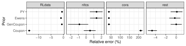
Figure 3: Posterior relative error in the predicted number of entities for all data sets and linkage structure priors. Under-linkage is observed for cora, which is likely due to significant noise that is not well-captured by the distortion model.

Distortion Model.

We compare our proposed distortion model (specified in the latter part of Section 3.1) to the distortion model proposed by Steorts (2015). For brevity, we refer to our distortion model as Ours and that of Steorts (2015) as blink. Here, we report results for the GenCoupon linkage structure prior – the results for the other linkage structure priors are reported in Appendix D and exhibit similar trends.

Figure 4 plots the inferred level of distortion for each attribute under both distortion models. It shows that blink tends to encourage high distortion, particularly for attributes with non-constant distance measures. For example, the fname_c1 and lname_c1 attributes for RLdata are predicted to be almost 100% distorted under the blink distortion model, which is inconsistent with expectations for this data set. Our distortion model does not appear to suffer from this problem, as it requires disagreement between entity and record attributes in order to classify them as “distorted”. Since high distortion makes reliable linkage more challenging, we expect that our distortion model is likely to perform better in practice. Indeed, it achieves a better balance between precision and recall in our full results (see Figure S7 in Appendix D).

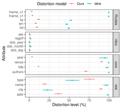
Figure 4: Comparison of the posterior attribute-level distortion under two distortion models: Ours (red top-most intervals) and blink (teal bottom-most intervals). The blink distortion model tends to favor higher levels of distortion – in some cases approaching 100 percent – which is not consistent with expectations.

Summary.

We return to the original goal of this section and summarize what we have learned in this study. First, we have learned that our proposed linkage structure prior is generally more robust due to the use of hyperpriors. In addition, our inferences are relatively insensitive to the EP parameter regime, which may be due to the fact that the data sets are relatively small in size. This behavior also holds for the blink distortion model when combined with our proposed linkage structure priors. Second, when studying the performance of the distortion models (blink versus our proposed distortion model), we find that ours predicts more reasonable distortion rates and improves the linkage accuracy as measured by F1 score. Thus, based on this study, we would recommend our distortion model and linkage structure priors moving forward for data sets similar to those we have considered. However, we stress that further exploration is needed to provide more general recommendations for other data sets.

5.4 Comparison with Baseline Models

In this section, we study how our entity resolution model performs in comparison with models by Steorts (2015) and (Sadinle, 2014). The blink model by Steorts (2015) is a natural baseline to consider, as it served as inspiration for our model. Compared to our model, blink is less Bayesian in its design, as many of the parameters are set empirically or arbitrarily. Both our model and blink, are examples of direct modeling approaches to ER – i.e., they model how the observed records are generated, incorporating the linkage structure as a latent variable. In contrast, the model by Sadinle (2014) (which we refer to as Sadinle) adopts a comparison-based approach to ER. Instead of modeling the data directly, it models attribute-level comparisons between pairs of records, incorporating the presence/absence of a link between the pair as a latent variable. Sadinle (2018) compares direct and comparison-based approaches from a methodological perspective, however we are not aware of any empirical comparisons in the literature. Our goal in this section is to provide a comparison for the first time on a variety of data sets, where we make no strong claims that our results generalize to all applications or data sets.

In order to make the comparison as fair as possible, we use the same distance functions to model the distortion in our model, blink, and Sadinle. For instance, if we use edit distance to model distortion for a name attribute in our model and blink, then we also use edit distance to compare the same name attribute in Sadinle. We set the distance cut-offs for our model and blink (see Section 4.3) to align with the blocking design used for Sadinle. Further information about our experimental setup is provided in Appendix E.

ER evaluation metrics are presented in Table 3 for all three models. For simplicity we only provide results for our model under the GenCoupon prior, which is denoted Ours in the table. Our model achieves the highest (or equal-highest) F1 score for all four data sets. We expect the poorer performance of blink is due to its use of subjective (inflexible) priors and its distortion model, which tends to favour high distortion and over-linkage. Sadinle achieves the second highest F1 score in the non-private setting (RLdata, cora, rest), and the lowest F1 score in the private setting (nltcs). The poorer performance for nltcs may be partly related to the blocking scheme, which is less aggressive, leaving the model more susceptible to over-linkage. Another important factor is the sensitivity of Sadinle to the truncation points for the priors on the $m$-probabilities. We perform coarse-grained tuning of the truncation points in Appendix F, however fine-grained tuning could result in additional performance gains.

		Evaluation metric
Data set	Model	Precision	Recall	F1 score
RLdata	Ours	0.917 (0.902, 0.932)	0.966 (0.953, 0.973)	0.934 (0.922, 0.942)
	blink	0.336 (0.327, 0.344)	0.992 (0.988, 0.996)	0.502 (0.492, 0.511)
	Sadinle	0.534 (0.524, 0.546)	0.964 (0.962, 0.966)	0.687 (0.679, 0.697)
nltcs	Ours	0.901 (0.878, 0.917)	0.934 (0.923, 0.943)	0.916 (0.903, 0.925)
	blink	0.904 (0.890, 0.918)	0.918 (0.904, 0.925)	0.910 (0.903, 0.918)
	Sadinle	0.312 (0.304, 0.319)	0.975 (0.969, 0.979)	0.473 (0.464, 0.480)
cora	Ours	0.973 (0.965, 0.980)	0.657 (0.627, 0.683)	0.784 (0.764, 0.803)
	blink	0.978 (0.970, 0.985)	0.219 (0.207, 0.234)	0.358 (0.341, 0.378)
	Sadinle	0.982 (0.981, 0.983)	0.359 (0.357, 0.362)	0.526 (0.524, 0.529)
rest	Ours	0.795 (0.749, 0.836)	0.830 (0.776, 0.871)	0.811 (0.774, 0.848)
	blink	0.635 (0.586, 0.671)	0.920 (0.893, 0.946)	0.751 (0.713, 0.780)
	Sadinle	0.993 (0.985, 1.000)	0.603 (0.598, 0.607)	0.750 (0.744, 0.756)

Table 3: Posterior performance of our model against two baselines: blink (Steorts, 2015) and Sadinle (Sadinle, 2014). A point estimate for each evaluation metric is reported based on the median, along with a 95% equi-tailed credible interval. Our model achieves the highest (or equal-highest) F1 score within the credible intervals for all data sets.

Summary.

This study provides evidence that our model achieves a better balance between precision and recall than blink and Sadinle. We stress that our results are based on four data sets – further experimentation is required to determine whether our results generalize to other data sets and applications. We speculate that the better performance of our model is mainly due to improved flexibility resulting from the addition of priors and hyperpriors, which can be viewed as performing model selection.

5.5 Controlled Simulation Study

We conduct a simulation study to evaluate our model under controlled conditions, where we vary the size of the data set, the level of distortion, and the level of duplication. Due to space constraints, we summarize the study here – full details can be found in Appendix C. We design a simulator for household survey data sets, where responses are collected for individuals within households. Since the attributes of individuals within a household are dependent – e.g., the address is the same, family members may share the same last name, the age of individuals may be correlated – the simulated data follows a more complex generative process than our entity resolution model. This is intentional, as it allows us to evaluate our model in a more realistic setting where it is misspecified for the data. The dataset simulator also incorporates a record generation process which is misspecified for our model. Rather than sampling individuals from the population, our data set simulator iterates over all individuals, randomly deciding whether to include the individual, and if so, how many distorted records to create.

We run entity resolution using our model on 16 simulated data sets, using the blink and Sadinle models as baselines. We summarize the results across three factors below:

• Duplication level. The level of duplication has minimal impact on the performance of our model. blink performs well for moderate to high levels of duplication, however it over-links severely when the level of duplication is low. The performance of Sadinle does not seem to follow a consistent trend as the duplication varies – it achieves a lower F1 score than our model and blink in all cases.

• Distortion level. We find the more distorted data sets are more difficult to link. Specifically, we observe a drop in recall of around 10 percentage points for our model and blink when compared to the data sets with low distortion. Larger drops in recall of 15–20 percentage points are observed for Sadinle.

• Data set size. We find that our model performs similarly for both data set sizes (1000 and 10000 records). blink also performs similarly in most scenarios, however, we observe a drop in precision for the larger data set when the level of duplication is low. Sadinle performs significantly worse for the larger data sets in terms of precision, however, the recall is relatively stable.

In summary, the simulation study shows that our model achieves the most consistent performance across all scenarios tested. blink is also competitive, but it is has poor performance in the low duplication scenario. Sadinle achieves the lowest F1 score when the level of duplication is non-negligible, and is somewhat competitive when the level of distortion is low.

6 Discussion

In this section, we summarize our contributions and provide a discussion regarding future work. We have proposed a Bayesian model for entity resolution that addresses limitations of previous work (Steorts et al., 2016; Steorts, 2015; Marchant et al., 2021). Our model can be viewed as performing graphical entity resolution, where observed records are clustered to (unobserved) latent entities. To improve upon the scalability of previous work, we designed a partially collapsed Gibbs sampler with an optimized implementation that can handle data sets of around 10,000 records. This allowed us to provide comparisons with models by Steorts (2015) and Sadinle (2014), which was previously only possible for toy-sized data sets. We provided comparisons to real and synthetic data sets and a controlled simulation study. We observed that our model tends to be less sensitive to changes in the hyperparameters than competing models for the data sets considered. Further analysis is required to make more general conclusions beyond the data sets and simulations considered in this paper.

There are many potential avenues for future work. First, it would be of interest to explore scaling for our proposed model and the model by Sadinle (2014). This could be achieved by designing parallel/distributed inference algorithms, by investigating more efficient MCMC algorithms, or by resorting to blocking techniques. Another area of interest, is exploring more diverse data sets to understand the strengths and weaknesses of each method in practice. Although we made recommendations based on four data sets and a simulation study, more comparisons would help to alleviate any selection bias regarding data sets and provide guidance to users. Finally, future work could consider microclustering priors (Miller et al., 2015) to assess their effectiveness compared to the infinitely-exchangeable linkage structure priors considered here. This would require modifying the sampling scheme and selecting an appropriate class of microclustering priors.

Acknowledgements

This work was supported by the National Science Foundation [CAREER-1652431], the Alfred Sloan Foundation, the Australian Research Council [DP220102269] and an Australian Government Research Training Program Scholarship.

Appendix A Gibbs Updates

In this appendix, we derive updates for the partially collapsed Gibbs sampler used to perform approximate inference for the ER model introduced in Section 3. Some of the updates are non-trivial due to non-conjugacy of the proposed model.

A.1 Update for the Distortion Probabilities

In this section, we provide the update for the distortion probability $\theta_{sa}$ (source $s$ and attribute $a$). This update is complicated by the presence of the distortion propensity variables $\omega_{ia}$, which breaks the conjugacy of the beta prior. To overcome this problem, we introduce the following auxiliary variables:

$$q_{ia}\mid\omega_{ia} \sim\operatorname{Bernoulli}(\omega_{ia}) \forall i,a$$

and modify the conditional distribution for the distortion indicators as follows:

$$z_{ia}\mid\theta_{\varsigma_{i}a},q_{ia} \sim\operatorname{Bernoulli}(\theta_{\varsigma_{i}a}q_{ia}) \forall i,a.$$

It is straightforward to show that one recovers the original model in Equation (5) when the auxiliary variables are marginalized out.

Observe that the contribution to the posterior involving $q_{ia}$ is

$$(\theta_{\varsigma_{i}a}q_{ia})^{z_{ia}}(1-\theta_{\varsigma_{i}a}q_{ia})^{1-z_{ia}}\omega_{ia}^{q_{ia}}(1-\omega_{ia})^{1-q_{ia}}=\left[\theta_{\varsigma_{i}a}^{z_{ia}}(1-\theta_{\varsigma_{i}a})^{1-z_{ia}}\omega_{ia}\right]^{q_{ia}}\left[1-\omega_{ia}\right]^{1-q_{ia}}.$$

Thus, the distribution of $q_{ia}$ conditional on the other variables is:

$$q_{ia}\mid\omega_{ia},\theta_{\varsigma_{i}a},z_{ia} \sim\operatorname{Bernoulli}\!\left(\frac{\omega_{ia}\theta_{\varsigma_{i}a}^{z_{ia}}(1-\theta_{\varsigma_{i}a})^{1-z_{ia}}}{\omega_{ia}\theta_{\varsigma_{i}a}^{z_{ia}}(1-\theta_{\varsigma_{i}a})^{1-z_{ia}}+1-\omega_{ia}}\right) \forall i,a.$$ (S15)

Next, observe that the contribution to the posterior involving $\theta_{sa}$ is

$$\theta_{sa}^{\beta_{sa}^{(0)}-1}(1-\theta_{sa})^{\beta_{sa}^{(1)}-1}\prod_{i:\varsigma_{i}=s}(\theta_{sa}q_{ia})^{z_{ia}}(1-\theta_{sa}q_{ia})^{1-z_{ia}}.$$

Hence, the distribution of $\theta_{sa}$ conditional on the other variables is:

$$\theta_{sa}\mid\bm{Q},\bm{Z},\bm{S} \sim\operatorname{Beta}\!\left(\beta_{sa}^{(0)}+\sum_{i:\varsigma_{i}=s}z_{ia},\ \beta_{sa}^{(1)}+\sum_{i:\varsigma_{i}=s}q_{ia}(1-z_{ia})\right) \forall s,a.$$ (S16)

It is also straightforward to see that the distribution of $z_{ia}$ conditional on the other variables is a point mass. In particular, we have

$$z_{ia}\mid x_{ia},\lambda_{i},\bm{Y}=\begin{cases}1,&\text{if }x_{ia}\neq y_{\lambda_{i}a}\\ 0,&\text{otherwise}\end{cases}$$ (S17)

In summary, to update the distortion probabilities, one would first compute the distortion indicators $\{z_{ia}\}$ using Equation (S17). Then, conditional on the other variables, one would draw auxiliary variables $\{q_{ia}\}$ using Equation (S15). Finally, one can update the distortion probabilities $\{\theta_{sa}\}$ using Equation (S16). The updates for the other model parameters are unaffected by the introduction of the auxiliary variables $\{q_{ia}\}$.

A.2 Update for the Entity Attributes

In this section, we provide the update for the entity attributes. When updating entity attribute $y_{ea}$, we collapse the base distribution $H_{ea}$ and distortion indicators $\bm{Z}$.

The posterior factors involving $y_{ea}$ after collapsing $H_{ea}$ are as follows:

$$P(y_{ea}\mid\bm{Z},\bm{\Omega},\bm{\Theta},\bm{S},G_{a},\rho_{a}) \propto P(y_{ea}\mid G_{a})$$

$$\qquad\times\int\prod_{i:\lambda_{i}=e}P(x_{ia}\mid\theta_{\varsigma_{i}a},\omega_{ia},y_{ea},H_{ea})P(H_{ea}\mid y_{ea},\rho_{a})\,\mathrm{d}H_{ea}$$

$$\propto P(y_{ea}\mid G_{a})\prod_{\begin{subarray}{c}i:\lambda_{i}=e\\ x_{ia}=y_{ea}\end{subarray}}(1-\theta_{\varsigma_{i}a}\omega_{ia})\prod_{\begin{subarray}{c}i:\lambda_{i}=e\\ x_{ia}\neq y_{ea}\end{subarray}}(\theta_{\varsigma_{i}a}\omega_{ia})$$

$$\qquad\times\int\prod_{\begin{subarray}{c}i:\lambda_{i}=e\\ x_{ia}\neq y_{ea}\end{subarray}}H_{ea}(x_{ia})\frac{\prod_{v\in\mathcal{D}_{a}\setminus\{y_{ea}\}}H_{ea}(v)^{\rho_{a}\psi_{a}(v\mid y_{ea})-1}}{\mathrm{B}(\rho_{a}\bm{\psi}_{a}(y_{ea}))}\,\mathrm{d}H_{ea}$$

$$\propto G_{a}(y_{ea})\prod_{\begin{subarray}{c}i:\lambda_{i}=e\\ x_{ia}=y_{ea}\end{subarray}}(1-\theta_{\varsigma_{i}a}\omega_{ia})\prod_{\begin{subarray}{c}i:\lambda_{i}=e\\ x_{ia}\neq y_{ea}\end{subarray}}(\theta_{\varsigma_{i}a}\omega_{ia})$$

$$\qquad\times\frac{\Gamma(\rho_{a})}{\Gamma(\bar{n}_{ea}(y_{ea})+\rho_{a})}\prod_{v\in\mathcal{V}_{ea}}\frac{\Gamma(n_{ea}(v)+\rho_{a}\psi_{a}(v\mid y_{ea}))}{\Gamma(\rho_{a}\psi_{a}(v\mid y_{ea}))},$$

where $\mathrm{B}(\cdot)$ is the multivariate beta function, $\mathcal{V}_{ea}=\left(\bigcup_{i:\lambda_{i}=e}\{x_{ia}\}\right)\setminus\{y_{ea}\}$ are the distorted record values for the $a$-th attribute associated with entity $e$, $n_{ea}(v)=\sum_{i:\lambda_{i}=e}\mathbb{1}[x_{ia}=v]$ is the number of records linked to entity $e$ whose $a$-th attribute is equal to $v$ and $\bar{n}_{ea}(v)=\sum_{i:\lambda_{i}=e}\mathbb{1}[x_{ia}\neq v]$ is the number of records linked to entity $e$ whose $a$-th attribute is not equal to $v$.

We can rewrite the above expression in a more computationally convenient form by repeatedly applying the recurrence relation for the Gamma functions to yield:

$$P(y_{ea}\mid\bm{Z},\bm{\Omega},\bm{\Theta},\bm{S},G_{a},\rho_{a}) \propto G_{a}(y_{ea})\frac{\prod_{v\in\mathcal{V}_{ea}}\prod_{j=1}^{n_{ea}(v)}\left\{j-1+\rho_{a}\psi_{a}(v\mid y_{ea})\right\}}{\prod_{j=1}^{\bar{n}_{ea}(y_{ea})}\left\{j-1+\rho_{a}\right\}}$$

$$\qquad\times\prod_{\begin{subarray}{c}i:\lambda_{i}=e\\ x_{ia}=y_{ea}\end{subarray}}(1-\theta_{\varsigma_{i}a}\omega_{ia})\prod_{\begin{subarray}{c}i:\lambda_{i}=e\\ x_{ia}\neq y_{ea}\end{subarray}}(\theta_{\varsigma_{i}a}\omega_{ia}).$$

Observe that the above distribution may only have support on a subset of the full domain $\mathcal{D}_{a}$ when distance thresholds are applied, as discussed in Section 4.3. In particular, one can show that the support is a subset of

$$\bigcap_{i:\lambda_{i}=e}\{y\in\mathcal{D}_{a}:\operatorname{dist}_{a}(y,x_{ia})\leq d_{a}^{(\mathrm{cut})}\}.$$

This fact can be used to implement the update more efficiently, since it is not necessary to construct a pmf over the entire domain $\mathcal{D}_{a}$.

A.3 Update for the Linkage Structure

In this section, we provide the update for the linkage structure. When updating the linkage structure, we use an urn-based scheme as described by Neal (2000). In doing so, we only need to keep track of entities in the population that are linked to records – any isolated entities not linked to records are ignored. This is important, as the population may be infinite in size for some Ewens-Pitman parameter regimes (when $\sigma\geq 0$).

To update the linked entity $\lambda_{i}$ for record $i$, we remove the current link and allow the record to either join one of the remaining instantiated entities (with at least one other record) or instantiate a “new” entity. The conditional distribution has the following form:

$$P(\lambda_{i}=e\mid\bm{Z},\bm{X},\bm{Y},\bm{\Lambda}_{-i},\{\rho_{a}\})\propto\begin{cases}C\frac{\lvert e\rvert-\sigma}{\alpha+N-1}\prod_{a}\int P(x_{ia}\mid z_{ia},y_{ea},H_{ea})\mathrm{d}\mathbb{H}_{-i,ea},\\ \mspace{100.0mu}\text{if $e$ is instantiated and $\lvert e\rvert>0$},\\ C\frac{\alpha+\sigma E}{\alpha+N-1}\prod_{a}\sum_{y_{ea}\in\mathcal{D}_{a}}P(y_{ea}\mid G_{a})\int P(x_{ia}\mid z_{ia},y_{ea},H_{ea})\mathrm{d}\mathbb{H}_{0,ea},\\ \mspace{100.0mu}\text{if $e$ is ``new''},\end{cases}$$ (S18)

where

• $C$ is a normalization constant;

• $\bm{\Lambda}_{-i}=(\lambda_{1},\ldots,\lambda_{i-1},\lambda_{i+1},\ldots,\lambda_{N})$ are the linked entities for all records excluding $i$;

• $\lvert e\rvert=\sum_{i^{\prime}\neq i}\mathbb{1}[\lambda_{i^{\prime}}=e]$ is the number of records (excluding $i$) linked to entity $e$;

• $E=\sum_{e^{\prime}\neq e}\mathbb{1}[\lvert e\rvert>0]$ is the number of instantiated entities with at least one linked record;

• $\mathbb{H}_{0,ea}$ is the prior for $H_{ea}$; and

• $\mathbb{H}_{-i,ea}$ is the posterior for $H_{ea}$ given the observed distorted record attributes $x_{i^{\prime}a}$ for which $i^{\prime}\neq i$ and $\lambda_{i^{\prime}}=e$ (also conditioned on $y_{ea}$ and $\rho_{a}$).

Recall that the prior $\mathbb{H}_{0,ea}$ for $H_{ea}$ conditioned on $y_{ea}$ and $\rho_{a}$ is $\operatorname{Dirichlet}(\rho_{a}\bm{\psi}_{a}(y_{ea}))$. Since $x_{ia}$ is $\operatorname{Categorical}(H_{ea})$ if $z_{ia}=1$ (and a point mass at $y_{ea}$ if $z_{ia}=0$), the posterior $\mathbb{H}_{-i,ea}$ is also Dirichlet by conjugacy. In particular, one can show that $\mathbb{H}_{-i,ea}$ is $\operatorname{Dirichlet}(\bm{\alpha}_{-i,ea})$ where

$$\alpha_{-i,ea}(v)=\rho_{a}\psi_{a}(v\mid y_{ea})+\sum_{i^{\prime}\neq i:\lambda_{i^{\prime}}=e}z_{i^{\prime}a}\mathbb{1}[x_{i^{\prime}a}=v]$$

for $v\in\mathcal{D}_{a}\setminus\{y_{ea}\}$. We can therefore simplify the integral in Equation (S18) with respect to $\mathbb{H}_{-i,ea}$ as follows:

$$\int P(x_{ia}\mid z_{ia},y_{ea},H_{ea})\,d\mathbb{H}_{-i,ea}$$

$$=\mathbb{1}[x_{ia}=y_{ea}]^{1-z_{ia}}\int H_{ea}(x_{ia})^{z_{ia}}\Gamma(\rho_{a})\prod_{v\in\mathcal{D}_{a}\setminus\{y_{ea}\}}\frac{H_{ea}(v)^{\rho_{a}\psi_{a}(v\mid y_{ea})-1}}{\Gamma(\rho_{a}\psi_{a}(v\mid y_{ea}))}\,\mathrm{d}H_{ea}$$

$$=\begin{cases}\frac{\alpha_{-i,ea}(x_{ia})}{\sum_{v\in\mathcal{D}_{a}\setminus\{y_{ea}\}}\alpha_{-i,ea}(v)},&z_{ia}=1\\ \mathbb{1}[x_{ia}=y_{ea}],&z_{ia}=0\end{cases}$$ (S19)

By a similar argument, the integral in Equation (S18) with respect to $\mathbb{H}_{0,ea}$ can be simplified to:

$$\int P(x_{ia}\mid z_{ia},y_{ea},H_{ea})\,d\mathbb{H}_{0,ea}=\begin{cases}\psi_{a}(x_{ia}\mid y_{ea}),&z_{ia}=1,\\ \mathbb{1}[x_{ia}=y_{ea}],&z_{ia}=0.\end{cases}$$ (S20)

Putting Equations (S19) and (S20) in (S18), then gives:

$$P(\lambda_{i}=e\mid\bm{Z},\bm{X},\bm{Y},\bm{\Lambda}_{-i},\{\rho_{a}\})\propto\begin{cases}C\frac{\lvert e\rvert-\sigma}{\alpha+N-1}\prod_{a:z_{ia}=1}\frac{\alpha_{-i,ea}(x_{ia})}{\sum_{v\in\mathcal{D}_{a}\setminus\{y_{ea}\}}\alpha_{-i,ea}(v)},\\ \mspace{100.0mu}\text{if $e$ is instantiated and $\lvert e\rvert>0$},\\ C\frac{\alpha+\sigma E}{\alpha+N-1}\prod_{a:z_{ia}=1}\sum_{y\in\mathcal{D}_{a}}G_{a}(y)\psi_{a}(x_{ia}\mid y)^{z_{ia}}\mathbb{1}[x_{ia}=y]^{1-z_{ia}},\\ \mspace{100.0mu}\text{if $e$ is ``new''}.\end{cases}$$

A.4 Update for the Ewens-Pitman Parameters

In this section, we describe the update for the Ewens-Pitman parameters. Since the priors on the Ewens-Pitman parameters $\alpha$ and $\sigma$ are non-conjugate, we cannot perform a direct Gibbs update. Thus, we describe tractable updates which require the introduction of auxiliary variables. The updates (and priors) differ depending on the range of $\sigma$. Teh (2006) proposed a scheme for beta/gamma priors when $0\leq\sigma<1$ and $\alpha>0$, which is summarized in Section A.4.1. In Section A.4.2 we propose a similar scheme for gamma/shifted negative binomial priors when $\sigma<0$.

A.4.1 Case $0\leq\sigma<1$ and $\alpha>0$

Teh (2006) proposed an auxiliary variable scheme for the regime $0\leq\sigma<1$ and $\alpha>0$ such that the priors

$$\sigma\sim\operatorname{Beta}\!\left(\zeta^{(0)},\zeta^{(1)}\right)\quad\text{and}\quad\alpha\sim\operatorname{Gamma}\!\left(\chi^{(0)},\chi^{(1)}\right)$$

are conjugate. We provide a summary of the scheme here, but refer the reader to (Teh, 2006) for further details. The scheme introduces the following sets of auxiliary variables conditional on the two parameters $\alpha$ and $\sigma$:

$$w\mid N,\alpha \sim\operatorname{Beta}(\alpha+1,N-1),$$ (S21)

$$u_{k}\mid\sigma,\alpha,E \sim\operatorname{Bernoulli}\!\left(\frac{\alpha}{\alpha+\sigma k}\right), k\in\{1,\ldots,E-1\}$$

$$v_{ej}\mid\sigma,\bm{\Lambda} \sim\operatorname{Bernoulli}\!\left(\frac{j-1}{j-\sigma}\right), \forall e,j\in\{1,\ldots,N_{e}-1\}.$$

Here $N_{e}=\lvert\{i:\lambda_{i}=e\}\rvert$ denotes the number of records linked to entity $e$, and $E=\sum_{e}\mathbb{1}[N_{e}>1]$ denotes the number of entities linked to at least one record.

It follows that the posterior distributions of $\alpha$ and $\sigma$ conditional on the auxiliary variables and other model parameter are given by:

$$\begin{split}\sigma\mid\{u_{k}\},\{v_{ej}\},\bm{\Lambda}&\sim\operatorname{Beta}\!\left(\zeta^{(0)}+\sum_{k=1}^{E-1}(1-u_{k}),\zeta^{(1)}+\sum_{e:N_{e}>1}\sum_{j=1}^{N_{e}-1}(1-v_{ej})\right),\\ \alpha\mid\{u_{k}\},w,\bm{\Lambda}&\sim\operatorname{Gamma}\!\left(\chi^{(0)}+\sum_{k=1}^{E-1}u_{k},\chi^{(1)}-\log w\right).\end{split}$$ (S22)

Thus, to update $\alpha$ and $\sigma$, one would first draw auxiliary variables $w$, $\{u_{k}\}$ and $\{v_{ej}\}$ conditional on the linkage structure $\bm{\Lambda}$ and the old values of $\alpha$ and $\sigma$ using Equation (S21). Then, conditional on the auxiliary variables and the linkage structure, one would draw new values for $\alpha$ and $\sigma$ using Equation (S22).

A.4.2 Case $\sigma<0$ and $\alpha=m\kappa$ for $m\in\mathbb{N}$

We describe an auxiliary variable scheme for updating the Ewens-Pitman parameters in the regime $\sigma<0$ and $\alpha=m\kappa$, where $m\in\mathbb{N}$ and $\kappa>0$. This scheme is inspired by Teh (2006). The likelihood factor associated with the partition of $N$ records into $E$ entities is as follows (Pitman, 2006):

$$P(\text{partition config})=\frac{(m)_{E\downarrow}}{(m\kappa)_{N\uparrow}}\prod_{e=1}^{E}(\kappa)_{N_{e}\uparrow}=\frac{\kappa^{E-1}(m-1)_{E-1\downarrow}}{(m\kappa-1)_{N-1\uparrow}}\prod_{e=1}^{E}(\kappa-1)_{N_{e}-1\uparrow},$$ (S23)

where “partition config” is a representation of the linkage structure $\bm{\Lambda}$ as a partition, $N_{e}$ is the number of records linked to the $e$-th entity, $(x)_{n\uparrow}=\prod_{i=0}^{n-1}(x+i)$ is the rising factorial, and $(x)_{n\downarrow}=\prod_{i=0}^{n-1}(x-i)$ is the falling factorial. We begin by expressing the denominator in this equation as

$$\frac{1}{(m\kappa-1)_{N-1\uparrow}}=\frac{\Gamma(m\kappa+1)}{\Gamma(m\kappa+N)} =\frac{\mathrm{B}(m\kappa+1,N-1)}{\Gamma(N-1)}$$

$$=\frac{1}{\Gamma(N-1)}\int_{0}^{1}w^{m\kappa}(1-w)^{N-2}\,\mathrm{d}w,$$

which allows us to introduce the following auxiliary variable:

$$w\mid m,\kappa,N\sim\operatorname{Beta}(m\kappa+1,N-1).$$ (S24)

Expressing each of the latter factors in Equation (S23) as

$$(\kappa-1)_{N_{e}-1\uparrow}=\prod_{j=1}^{N_{e}-1}(\kappa+j)=\prod_{j=1}^{N_{e}-1}\sum_{v_{ej}\in\{0,1\}}\kappa^{v_{ej}}j^{1-v_{ej}}$$

permits us to introduce the following additional auxiliary variables:

$$v_{ej}\mid\kappa \sim\operatorname{Bernoulli}\!\left(\frac{\kappa}{\kappa+j}\right), \forall e,j\in\{1,\ldots,N_{e}-1\}.$$ (S25)

With this representation, we can place conjugate priors on $\kappa$ and $m$, namely:

$$\kappa\sim\operatorname{Gamma}(\chi^{(0)},\chi^{(1)})\ \text{and}\ m\sim\operatorname{NegativeBinomial}(r,\nu)+1.$$ (S26)

The distribution on $m$ is a shifted negative binomial with support on the positive integers. The parameterization we adopt for the negative binomial is in terms of the number of failures $x\in\{0,1,2,\ldots\}$ in a sequence of trials before a given number of successes $r>0$ occur. Each trial is an i.i.d. draw from a Bernoulli distribution with success probability $\nu$. The density of $x$ is given by

$$P(x\mid r,\nu)=\frac{(x+r-1)!}{(r-1)!x!}\nu^{r}(1-\nu)^{x}.$$

Finally, we combine the priors in Equation (S26) with the likelihood factors to obtain the following posterior distributions for the $m$ and $\kappa$, conditional on the other model parameters:

$$m\mid w,\kappa,\bm{\Lambda} \sim\operatorname{NegBinomial}\!\left(r+E-1,1-(1-\nu)w^{\kappa}\right)+E,$$ (S27)

$$\kappa\mid\{v_{ej}\},w,m,\bm{\Lambda} \sim\operatorname{Gamma}\!\left(\chi^{(0)}+E-1+\sum_{e=1}^{E}\sum_{j=1}^{N_{e}-1}v_{ej},\ \chi^{(1)}-m\log w\right).$$

Thus, to update $\kappa$ and $m$, one would first draw auxiliary variables $w$ and $\{v_{ej}\}$ conditional on the linkage structure $\bm{\Lambda}$ and the old values of $\alpha$ and $\sigma$ using Equations (S24) and (S25). Then, conditional on the auxiliary variables and the linkage structure, one would draw new values for $\kappa$ and $m$ using Equation (S27).

A.5 Update for the Distortion Distribution Concentration

In this section, we provide the update for the distortion distribution concentration $\rho_{a}$. Since we cannot rely on conjugacy for the update, we propose an auxiliary variable scheme. When updating $\rho_{a}$, we condition on the entity attribute values $\{y_{ea}\}_{e=1\ldots E}$, the record attribute values $\{x_{ia}\}_{i=1\ldots N}$ and the links $\bm{\Lambda}=\{\lambda_{i}\}_{i=1\ldots N}$. We collapse the distortion distributions $\{H_{ea}\}_{e=1\ldots E}$. The contribution to the likelihood involving $\rho_{a}$ is:

$$\prod_{e}\int\prod_{i:\lambda_{i}=e}P(x_{ia}\mid\theta_{\varsigma_{i}a},\omega_{ia},y_{ea},H_{ea})P(H_{ea}\mid\rho_{a})\,\mathrm{d}H_{ea}$$

$$\propto\prod_{e}\frac{\Gamma(\rho_{a})}{\Gamma(\bar{n}_{ea}(y_{ea})+\rho_{a})}\prod_{v\in\mathcal{V}_{ea}}\frac{\Gamma(n_{ea}(v)+\rho_{a}\psi_{a}(v\mid y_{ea}))}{\Gamma(\rho_{a}\psi_{a}(v\mid y_{ea}))}$$

$$=\prod_{e}\frac{\mathrm{B}(\rho_{a},\bar{n}_{ea}(y_{ea}))}{\Gamma(\bar{n}_{ea}(y_{ea}))}\prod_{v\in\mathcal{V}_{ea}}\prod_{j=1}^{n_{ea}(v)}\{j-1+\rho_{a}\psi_{a}(v\mid y_{ea})\}$$ (S28)

where $\mathrm{B}(\cdot,\cdot)$ is the beta function, $\mathcal{V}_{ea}:=\left(\bigcup_{i:\lambda_{i}=e}\{x_{ia}\}\right)\setminus\{y_{ea}\}$, $n_{ea}(v)=\sum_{i:\lambda_{i}=e}\mathbb{1}[x_{ia}=v]$ and $\bar{n}_{ea}(v)=\sum_{i:\lambda_{i}=e}\mathbb{1}[x_{ia}\neq v]$.

Expressing the beta function in Equation (S28) as

$$\mathrm{B}(\rho_{a},\bar{n}_{ea}(y_{ea}))=\int_{0}^{1}w_{e}^{\rho_{a}-1}(1-w_{e})^{\bar{n}_{ea}(y_{ea})-1}\,\mathrm{d}w_{e}$$

permits us to introduce the following auxiliary variables:

$$w_{e}\mid\rho_{a},\bm{X},\bm{Y},\bm{\Lambda}\sim\operatorname{Beta}\!\left(\rho_{a},\sum_{e}\sum_{i}\mathbb{1}[x_{ia}\neq y_{\lambda_{i}a}]\right),$$

for all $e$. We can also express each of the latter factors in Equation (S28) as

$$j-1+\rho_{a}\psi_{a}(v\mid y_{ea})=\sum_{u_{evj}=0}^{1}\rho_{a}\psi_{a}(v\mid y_{ea})^{u_{evj}}(j-1)^{1-u_{evj}}$$

which permits us to introduce the following auxiliary variables:

$$u_{evj}\mid\rho_{a},\bm{X},\bm{Y},\bm{\Lambda} \sim\operatorname{Bernoulli}\!\left(\frac{\rho_{a}\psi_{a}(v\mid y_{ea})}{j-1+\rho_{a}\psi_{a}(v\mid y_{ea})}\right)$$ (S29)

for all $e$, $v\in\mathcal{V}_{ea}$ and $j\in\{1,\ldots,n_{ea}(v)\}$.

Now since the prior on $\rho_{a}$ is $\operatorname{Gamma}(\tau_{a}^{(0)},\tau_{a}^{(1)})$, we obtain the following posterior distribution for $\rho_{a}$ conditional on the other parameters:

$$\rho_{a}\mid\{w_{e}\},\{u_{evj}\},\bm{X},\bm{Y},\bm{\Lambda}\sim\operatorname{Gamma}\!\left(\tau_{a}^{(0)}+\sum_{e}\sum_{v\in\mathcal{V}_{ea}}\sum_{j=1}^{n_{ea}(v)}u_{evj},\tau_{a}^{(1)}-\sum_{e}\log w_{e}\right).$$ (S30)

Thus to update $\rho_{a}$, one would first draw auxiliary variables $\{w_{e}\}$ and $\{u_{evj}\}$ conditional on the record attributes $\bm{X}$, entity attributes $\bm{Y}$, linkage structure $\bm{\Lambda}$, and the previous value of $\rho_{a}$ using Equations (A.5) and (S29). Then, conditional on the auxiliary variables and $\bm{X}$, $\bm{Y}$, $\bm{\Lambda}$, one would draw a new value for $\rho_{a}$ using Equation (S30).

Appendix B Hybrid Distance Measure

In this appendix, we describe a hybrid distance measure that is useful for comparing text strings containing multiple tokens (words), where individual tokens may be subject to distortion. We use the measure in this paper for comparing name and address attributes in the cora and rest data sets (see Section 5.1), however it may have wider applications beyond this paper. Our measure draws inspiration from a hybrid similarity measure proposed by Monge and Elkan (1996). However, unlike Monge and Elkan, we attempt to match the tokens in each string while incorporating penalties for tokens that are “missing” in one of the strings.

Suppose we would like to compare a pair of multi-token strings $x$ and $y$. As a running example, we consider $x=$ “University of California, San Diego” and $y=$ “Univ. Calif., San Diego”. Given a separator character (e.g., a space), we can map each string to a set of tokens. For example, string $x$ from our running example would be mapped to

$$X=\{\text{``California,'', ``Diego'', ``of'', ``San'', ``University''}\}.$$

Note that we have used capital $X$ to denote the token set representation of string $x$ – a convention we adopt throughout this appendix. Also note that $X$ is a lossy representation of $x$, as it discards information about the token order. This is desirable for our applications to names and addresses, where permutation of the tokens does not significantly change the meaning of the strings.

We propose to measure the distance from $x$ to $y$ via a generalized edit distance on the token sets $X$ and $Y$. We consider three elementary edit operations:

• token insertions where a token $b$ is appended to the input set;

• token deletions where a token $a$ is removed from the input set; and

• token substitutions where a token $a$ in the input set is replaced by a token $b\neq a$.

Each elementary operation takes an input set $Q$ to an output set $Q^{\prime}$, which we write as $Q\to Q^{\prime}$, and has an associated cost $c(Q\to Q^{\prime})\geq 0$. We let

$$c(Q\to Q^{\prime})=\begin{cases}d_{i}\,\operatorname{dist}_{\mathrm{inner}}(\lambda,b),&\text{if $Q=Q^{\prime}\setminus\{b\}$ (insertion),}\\ d_{d}\,\operatorname{dist}_{\mathrm{inner}}(a,\lambda),&\text{if $Q\setminus\{a\}=Q^{\prime}$ (deletion),}\\ d_{s}\,\operatorname{dist}_{\mathrm{inner}}(a,b),&\text{if $Q\setminus\{a\}=Q^{\prime}\setminus\{b\}$ (substitution),}\end{cases}$$

where $d_{i},d_{d}$ and $d_{s}$ are non-negative weights; $\lambda$ is the null string; and $\operatorname{dist}_{\mathrm{inner}}(\cdot,\cdot)$ is an inner distance measure on tokens (strings). We then define the hybrid distance between $x$ and $y$ as the minimum average cost of transforming $X$ into $Y$ via a sequence of elementary edit operations $T_{X,Y}=(X\to Q_{1},Q_{1}\to Q_{2},\ldots,Q_{l-1}\to Y)$. Symbolically, we write

$$\operatorname{dist}_{\mathrm{hybrid}}(x,y)=\min_{T_{X,Y}}\frac{1}{\lvert T_{X,Y}\rvert}\sum_{(Q\to Q^{\prime})\in T_{X,Y}}c(Q\to Q^{\prime}).$$

We can compute the hybrid distance using an off-the-shelf linear sum assignment problem (LSAP) solver (Crouse, 2016). In order to do so, we need to add null string tokens to $X$ and $Y$ to account for all possible insertion and deletion operations. Concretely, we add $\lvert Y\rvert$ null tokens to $X$ to allow for insertions and $\lvert X\rvert$ null tokens to $Y$ to allow deletions. We then construct a pairwise cost matrix by applying $\operatorname{dist}_{\mathrm{inner}}$ to all pairs of tokens in (the amended) $X$ and $Y$. The resulting matrix is then passed to the LSAP solver, which returns the optimal set of edit operations and their cost.

Returning to our running example, if we set $\operatorname{dist}_{\mathrm{inner}}$ to the Levenshtein distance, the solution to the LSAP is

$$\{(\text{``University''}\leftrightarrow\text{``Univ.''},5),(\text{``of''}\leftrightarrow\lambda,2),(\text{``California,''}\leftrightarrow\text{``Calif.,''},6),$$

$$(\text{``San''}\leftrightarrow\text{``San''},0),(\text{``Diego''}\leftrightarrow\text{``Diego''},0),(\lambda\leftrightarrow\lambda,0),(\lambda\leftrightarrow\lambda,0),$$

$$(\lambda\leftrightarrow\lambda,0),(\lambda\leftrightarrow\lambda,0)\}.$$

Hence we conclude that $\operatorname{dist}_{\mathrm{hybrid}}(x,y)=\frac{5+2+6+0+0}{5}=2.6$. This distance reflects the semantic closeness between $x$ and $y$ better than the Levenshtein distance, which gives a larger value of 14 when evaluated directly on $x$ and $y$.

Appendix C Simulation Study

In this appendix, we conduct a simulation study to understand how our model performs in controlled scenarios. Specifically, we simulate entity resolution data sets where we vary the number of records, the level of distortion and the level of duplication. Since our model is generative, we could use it to simulate data, however the resulting data would have negligible specification error for our model, which is not realistic. We therefore simulate data that is purposefully misspecified for our model by adding additional dependencies between the entities and entity attributes, and by using a different process to generate records from entities. We were unable to find an existing data set simulator that generated such data, so we implemented our own.

C.1 Data Set Simulator

We provide an overview of our simulator, which generates personal records describing a population of households. For brevity, we omit low-level details here and refer the reader to the included Python script. Our simulator operates in two stages: in the first stage it generates a population of households, then in the second stage it iterates over individuals in all households, generating a random number of distorted records for each individual. By generating households rather than individuals in the first stage, we are able to incorporate additional dependencies between individuals (entities) that are not present in our ER model (see Section 3.1).

Generating Households.

We now describe how households are generated in the first stage. In our simplified model, a household may be a couple, a single, a couple or single with children, or a group of unrelated adults. Individuals within a household are described by the following attributes: first and last name (first_name and last_name), date of birth (birth_year, birth_month, birth_day), gender and zipcode. The zipcode is constrained to be the same for all individuals within a household, and the first name is conditioned on the gender, however the other attributes may vary as described below. Random values for attributes are generated using the Faker Python library, which attempts to mimic real-world frequency distributions. We make the distributions more concentrated for the name and zipcode attributes to ensure the entities are not too unique (otherwise entity resolution would be too easy).

We begin by generating the head(s) of the household, which are a male and female couple (for simplicity) or a single male or female. If a couple is generated, they have a high chance of sharing the same last name and their birth years are likely not too far apart. Next we randomly decide whether to generate children. If children are generated, they share the same last name as the head(s) of the household (the parents) and there is an appropriate gap between their birth year and their parents’ birth year. If no children are generated, then we randomly decide whether to generate unrelated adults who live with the head(s) of household. The unrelated adults are constrained to be of a similar age as the head(s) of the household. When simulating the household composition, we attempt to follow aggregate statistics from the Current Population Survey (U.S. Census Bureau, 2016).

Generating Records.

In the second stage, records are generated for individuals across all households. We simulate a single database/file with duplicate records by including an individual with probability $p_{\mathrm{inc}}=0.9$ and sampling the number of records according to a Poisson distribution with rate parameter $\mu$, truncated to the interval $[1,4]$. Each record is obtained by copying the entity attributes subject to distortion. This is done by iterating over the attributes in a random order, and deciding whether to activate the distortion process with a probability that varies for each attribute. The distortion process for birth day, birth month, gender and zipcode involves drawing a replacement value according to the distribution used in the first stage. The distortion process for birth year involves adding discrete Gaussian noise to the true birth year. The distortion process for first and last name may proceed in one of three ways: (1) by making a random typographical error (character insertion, deletion, substitution or transposition); (2) by replacing the name with a variant drawn uniformly at random; or (3) by generating a replacement according to the distribution used in the first stage. Variant names for (2) are sourced from the WeRelate.org Variant Names Project.

C.2 Results

We generate 16 data sets using our simulator for each combination of the following variables:

• Number of records. We consider data sets with 1000 and 10000 records in expectation. The number of records is random and depends on the number of individuals and the Poisson rate parameter. Since the Poisson rate parameter is fixed (see below), we control the number of records by varying the number of individuals generated in the first stage.

• Level of distortion. We consider two levels of record distortion which we refer to as “low” and “high”. These correspond to different choices for the probabilities of activating the distortion process as detailed in Table S4.

• Level of duplication. We consider four levels of duplication which we refer to as “low”, “medium”, “high” and “very high”. These levels correspond to Poisson rate parameters of 0.1, 1, 8 and 100, respectively. When the duplication is “low” ($\mu=0.1$) over 95% of the entities represented in the data only appear once. Whereas when the duplication is “very high” ($\mu=100$) over 95% of the entities represented in the data appear four times. The distribution of records per entity is plotted for each level in Figure S5.

	Distortion probability
Attribute	Low distortion	High distortion
first_name	10%	40%
last_name	10%	40%
gender	1%	1%
zipcode	5%	10%
birth_year	1%	10%
birth_month	1%	10%
birth_day	1%	10%

Table S4: Attribute-level distortion probabilities for two levels of distortion: low and high.

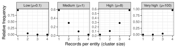
Figure S5: Distribution of records per entity for each level of duplication: low, medium, high and very high. The Poisson rate parameter $\mu$ for each level is given in parentheses.

We perform a comparative evaluation of our model, blink, and Sadinle on the 16 simulated data sets. The model evaluation procedure is described in Section 5.2 and the blink and Sadinle models are introduced in Section 5.4. ER evaluation metrics are plotted for each data set in Figure S6. We now make several observations about the results.

First, we observe that our model and blink perform similarly when the duplication level is medium, high or very high. For these duplication levels, blink has a slight advantage in terms of recall when the distortion level is high. The largest difference is observed for the medium duplication/high distortion scenario, where the recall for blink is roughly 10 percentage points higher than for our model. This difference is due to the priors placed on the concentration parameters $\rho_{a}$ in our model, which favour high concentrations. This corresponds to a prior belief that distortions occur in the same way, rather than in multiple different ways. However, this is not true for distortions in the simulated data – e.g., an individual whose first name is “JONATHON” may appear in the data with four distinct first names: “JOHN”, “JOJN”, “JONATHON” and “ALEX”. If we wanted to exploit this knowledge, we could increase $\tau_{a}^{(0)}$ for our model to favour lower concentrations.

Second, we observe that our model significantly outperforms blink in terms of precision when the duplication level is low. We believe this is due to the highly informative prior on the linkage structure used in blink – it uses a coupon prior with $m$ fixed to the number of records $N$ and $\kappa\to\infty$. However our model under the generalized coupon prior selects a value for $m$ of approximately $8\times N$ and $\kappa$ of approximately 100, which allows it to more accurately model a low duplication scenario.

Thirdly, we observe that Sadinle achieves the lowest F1 score when the duplication level is medium, high or very high. For these duplication levels, the performance gap in F1 score is largest when the distortion is high – approximately 20 percentage points. The gap is less significant when the distortion is low – around 5 percentage points. These differences in F1 score are mainly due to lower recall in most cases – the precision is generally competitive with the other models.

Fourthly, we comment on the effect of the dataset size, measured in terms of the expected number of records (1000 or 10000). We observe similar trends for all three models: the precision tends to be larger for the smaller dataset, while the recall tends to be larger for the larger dataset (however there are exceptions). The difference in performance is most pronounced for the low duplication setting, where the precision of blink and Sadinle drops considerably for the larger dataset, and the recall of Sadinle drops also drops considerably for the larger dataset.

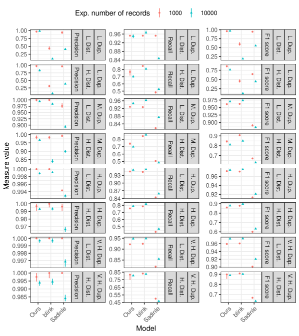
Figure S6: Posterior evaluation metrics for our model, blink, and Sadinle when fitted on simulated datasets with varying levels of distortion and duplication. Low and high distortion levels are abbreviated as “L. Dist.” and “H. Dist.” respectively. Low, medium, high and very high duplication levels are abbreviated as “L. Dup.”, “M. Dup.”, “H. Dup.” and “V. H. Dup.” respectively. The expected number of records (1000 or 10000) is denoted by the color and shape of the markers. A point estimate for each evaluation metric is reported based on the median and 95% equi-tailed credible interval are represented by intervals around the point.

Appendix D Study of Linkage Structure Priors and the Distortion Model

In this appendix, we provide additional results for the study of linkage structure priors and distortion models presented in Section 5.3. Our goal is to study the impact of the modeling contributions independently, to determine whether each contribution is beneficial in its own right, and/or whether one contribution is more beneficial than the other.

Recall from Section 5.3 that we considered four parameter regimes for the linkage structure priors – PY, Ewens, GenCoupon and Coupon – and two distortion models – Ours as proposed in Section 3.1 and blink as proposed by Steorts (2015). Thus, there are eight model variants to test – one for each linkage structure prior and distortion model. Figure S7 presents pairwise evaluation metrics (F1 score, precision and recall) for the eight model variants and four data sets in a single plot. We interpret the results for each modeling contribution below.

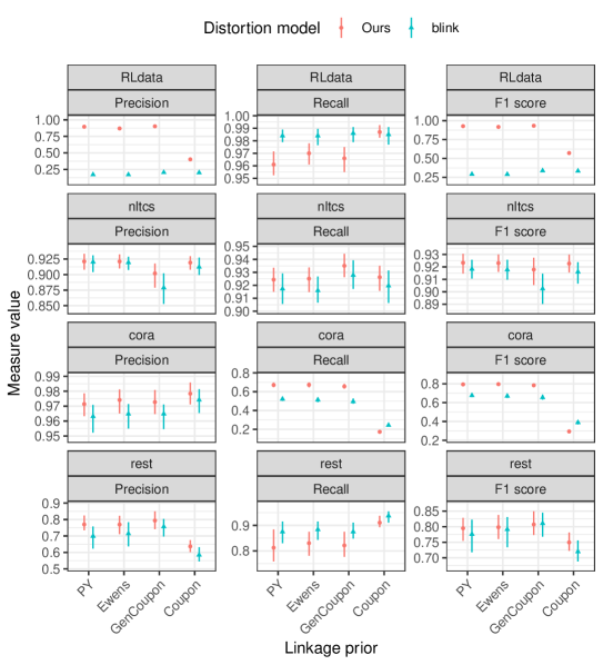
Figure S7: Evaluation of ER quality as a function of the linkage structure prior (plotted on the $x$-axis) and distortion model (indicated by the line color). Three pairwise evaluation measures are shown (grouped by column) for four data sets (grouped by row).

Linkage Structure Prior.

While we discuss the effect of the linkage structure prior in Section 5.3, we only present results for our distortion model (Ours) due to space constraints. In Section 5.3, we draw two main conclusions from the results in Table 2 which are replicated in Figure S7 (represented by circular vermilion markers):

1. Our proposal to place vague hyperpriors on the EP parameters (for PY, Ewens and GenCoupon) improves robustness and yields the highest ER accuracy for three of data sets, as measured by pairwise F1 score (nltcs is the exception). We observe significantly lower F1 scores when hyperpriors are not used (see Coupon in Figure S7), particularly for cora and RLdata. Figure S8 provides further justification for this argument, as it shows vastly different values of the EP parameters are selected for each data set, facilitated by the vague hyperpriors.

2. Our inferences are relatively insensitive to the EP parameter regime (PY, Ewens or GenCoupon) despite the fact that each regime is known to exhibit distinct asymptotic behavior (see Section 2.2).

Figure S7 shows that these conclusions also hold for the blink distortion model (represented by triangular teal markers). We expect the competitive performance for nltcs under the Coupon linkage prior may be a coincidence, as the population size under the prior is 3,387, which happens to be very close to the true value of 3,307 (see Table 1).

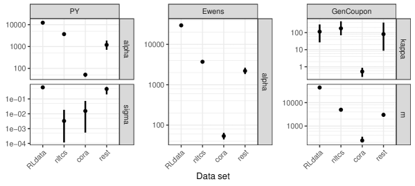
Figure S8: Posterior Ewens-Pitman parameters for three regimes: PY, Ewens and GenCoupon under our distortion model (Ours). Note that the values of the parameters are presented on log-scales.

Distortion Model.

In Section 5.3, we discuss the effect of the distortion prior under the GenCoupon linkage structure prior. We now extend the discussion to include results for the three other linkage structure priors (PY, Ewens and Coupon), as presented in Figure S7.

We find that our distortion model achieves the highest F1 score for all but one of the data sets and linkage structure priors. The exception is for cora under the Coupon linkage structure prior, where the blink distortion model has a slight edge. An explanation for the improved performance of our model is given in Section 5.3, which we summarize here. The blink distortion model is susceptible to entering a high distortion mode, particularly for attributes with non-constant distance measures. This is because it allows a record attribute value to be marked as “distorted” even if it is not actually distorted. Our model corrects this inconsistency, and in doing so appears to be more robust. In general, we expect the blink distortion model to result in over-linkage (high recall, low precision), while our model is expected to be more balanced. Figure S7 supports this argument, with the difference being most apparent for RLdata, where we see a difference of $\sim$0.7 in the F1 score.

Appendix E Further Details of Experimental Setup

In this appendix, we provide further details about the experiments presented in Section 5.

Implementation and Hardware.

All experiments were conducted in R version 3.4.4, running on a local server fitted with two 28-core Intel Xeon Platinum 8180M CPUs and 12 TB of RAM. We developed an open-source R package called exchanger which implements variants of our model (under different linkage structure priors and distortion models) in addition to the blink model (Steorts, 2015). Since an implementation of the model proposed by Sadinle (2014) was not publicly available, we developed our own which we released as an open-source R package called BDD. For efficiency reasons, we implemented inference for all models in C++ using the Rcpp interface (Eddelbuettel and François, 2011). The data set simulator described in Appendix C.1 was implemented as a Python script. A Pipfile is provided to specify the dependencies used when running the script.

Hyperparameter Settings.

We followed the recommendations in Section 3.2 when setting hyperparameters for our model. When setting hyperparameters for the two baseline models, we attempted to follow the recommendations of the authors. For blink, we set $m=N$ for the coupon-collector’s prior and $\beta_{sa}^{(0)}=N/1000$ and $\beta_{sa}^{(1)}=N/10$ for the Beta prior on the distortion probabilities (here $N$ is the total number of records). For Sadinle, we set the agreement levels by inspecting the distribution of distances for each attribute. We used truncated uniform priors on the $m$-probabilities and a uniform prior on the $u$-probabilities, as recommended by the author. We set the lower truncation points for the $m$-probabilities to 0.95, based on tuning experiments presented in Appendix F.

Initialization and MCMC.

For our model and blink, we initialized the linkage structure $\bm{\Lambda}$, entity attributes $\bm{Y}$ and distortion indicators $\bm{Z}$ by linking each record to a unique entity and copying the record attributes into the entity attributes, assuming no distortion. The distortion probabilities $\bm{\Theta}$ and entity attributes distributions $\bm{G}$ were initialized by drawing from their conditional distributions. The Ewens-Pitman parameters and distortion distribution concentration parameters were initialized using their prior means.

A similar initialization was used for the Sadinle model. We assigned each record to a unique entity (cluster). The $m$- and $u$-probabilities were initialized by drawing from their conditional distributions.

When fitting each model, we ran Markov chain Monte Carlo (MCMC) for $2\times 10^{5}$ iterations, discarding the first $10^{5}$ iterations as burn-in, and applying thinning with an interval of 10. This produced $10^{4}$ approximate posterior samples.

Appendix F Tuning Hyperparameters for Sadinle (2014)

Our aim in this appendix is to determine reasonable values for the hyperparameters in the entity resolution model by Sadinle (2014), which we refer to as Sadinle. We assume the distance functions (used to compare attributes) and agreement levels (mappings from real-valued distances to discrete levels) are fixed, and that flat priors are used, as recommended by Sadinle. Given these assumptions, the only hyperparameters that remain unspecified are the lower truncation points for the $m$-probabilities.

The $m$-probabilities are a set of parameters $\{m_{al}\}$ where $m_{al}$ is the probability that a pair of records referring to the same entity agree at level $l$ on attribute $a$, given they do not agree at levels $0,1,\ldots,l-1$. Sadinle recommends using truncated flat priors on $m_{al}$, so that the allowed values lie in the interval $[\lambda_{al},1]$, where $\lambda_{al}\in[0,1]$ is a hyperparameter typically close to 1. More specifically, he recommends setting $\lambda_{al}=0.95$ if attribute $a$ is a “nearly-accurate” quasi-identifier and $\lambda_{al}=0.85$ if attribute $a$ is an “inaccurate” quasi-identifier. Since it is not clear which setting for $\lambda_{al}$ is best for our data sets, we run the experiments described in Section 5.4 for four different values: $\lambda_{al}=0,0.5,0.85,0.95$. When setting $\lambda_{al}$, we use the same value for all attributes $a$ and agreement levels $l$ for simplicity. The results are reported in Figure S9 and Table S5.

Figure S9 plots the posterior values of the $m$-probabilities (on the $x$-axis) for each truncation point $\lambda_{al}$ (corresponding to the horizontal panels). We observe that the posterior values of $m_{al}$ tend to be close to $\lambda_{al}$, especially for agreement level $l=0$ and $\lambda_{al}\geq 0.5$. This suggests that the model favors small values of $m_{al}$, despite the fact that $m_{al}$ is expected to be close to 1. Consequently, the model has a tendency to “over-link”—linking records that do not refer to the same entity. Understanding why the model exhibits this behavior would require further exploration and is beyond the scope of this paper. However, we speculate that it may be related to the use of flat priors, or known stability issues with Fellegi-Sunter-type models (Goldstein et al., 2017). As a result, we conclude that the posterior value of $m_{al}$ is highly sensitive to the choice of $\lambda_{al}$.

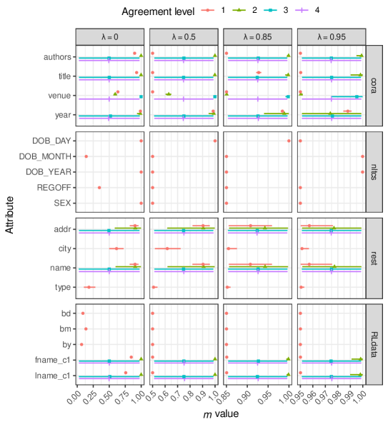
Figure S9: Posterior estimates of the $m$-probabilities (plotted on the $x$-axis) in the Sadinle model as a function of the data set (vertical panels), attribute ($y$-axis), agreement level (color/marker) and lower truncation point (horizontal panels). Point estimates are shown based on the median, along with 95% equi-tailed credible intervals. The model has a tendency to select small values for the $m$-probabilities, close to the lower truncation point, especially for agreement level 1.

Table S5 shows the impact of the truncation point $\lambda_{al}$ on entity resolution performance. It shows that the performance is relatively stable for cora and rest as a function of $\lambda_{as}$, despite the fact that there is some variation in the $m$-probabilities (as shown in Figure S9). The reason for the stability may be related to the blocking scheme used for these data sets, which rules out a relatively large number of potential links, thereby guarding against over-linkage. On the other hand, the performance for RLdata and nltcs is far less stable. We find that the precision drops considerably as $\lambda_{al}$ is reduced, while the recall remains relatively stable. This is a sign of over-linkage, which is expected since the posterior $m$-probabilities are significantly smaller. Based on these results, we set $\lambda_{al}=0.95$ as the default value for our other experiments since it seems to achieve balanced performance.

		Evaluation metric
Data set	Truncation point	Precision	Recall	F1 score
RLdata	0.00	0.068 (0.067, 0.068)	0.909 (0.906, 0.912)	0.126 (0.125, 0.126)
	0.50	0.069 (0.069, 0.069)	0.921 (0.919, 0.924)	0.128 (0.128, 0.129)
	0.85	0.315 (0.308, 0.321)	0.965 (0.962, 0.967)	0.475 (0.467, 0.481)
	0.95	0.534 (0.524, 0.546)	0.964 (0.962, 0.966)	0.687 (0.679, 0.697)
nltcs	0.00	0.114 (0.113, 0.114)	0.983 (0.978, 0.987)	0.204 (0.203, 0.205)
	0.50	0.111 (0.110, 0.111)	0.964 (0.958, 0.970)	0.199 (0.197, 0.200)
	0.85	0.162 (0.160, 0.164)	0.972 (0.968, 0.976)	0.278 (0.275, 0.281)
	0.95	0.312 (0.304, 0.319)	0.975 (0.969, 0.979)	0.473 (0.464, 0.480)
cora	0.00	0.980 (0.979, 0.981)	0.378 (0.377, 0.378)	0.545 (0.544, 0.546)
	0.50	0.981 (0.979, 0.984)	0.390 (0.389, 0.391)	0.558 (0.557, 0.560)
	0.85	0.984 (0.983, 0.984)	0.383 (0.382, 0.384)	0.552 (0.551, 0.553)
	0.95	0.982 (0.981, 0.983)	0.359 (0.357, 0.362)	0.526 (0.524, 0.529)
rest	0.00	1.000 (0.985, 1.000)	0.607 (0.598, 0.607)	0.756 (0.744, 0.756)
	0.50	0.985 (0.985, 1.000)	0.598 (0.598, 0.607)	0.744 (0.744, 0.756)
	0.85	0.985 (0.985, 1.000)	0.598 (0.598, 0.607)	0.744 (0.744, 0.756)
	0.95	0.993 (0.985, 1.000)	0.603 (0.598, 0.607)	0.750 (0.744, 0.756)

Table S5: Posterior performance of the Sadinle model as a function of the lower truncation point $\lambda_{al}$ on the $m$-probabilities. A point estimate for each evaluation metric is reported based on the median, along with a 95% equi-tailed credible interval.

Appendix G MCMC Diagnostics

G.1 Study of Linkage Structure Priors

Here we present convergence diagnostics for the models fitted in Section 5.3. We present Geweke diagnostic plots and trace plots for a selection of model variables for each data set, linkage structure prior and distortion model. Each pair of plots is preceded by a title of the form “Data set — Linkage structure prior — Distortion model”. The Geweke diagnostic plot (on the left) depicts a Z-score on the x-axis for each variable on the y-axis. The Z-score tests for equality of the means of the first 10% and final 50% of the Markov chain, and is typically expected to be in the range $[-2,2]$ (Geweke, 1992). The trace plot (on the right) depicts the value of variables (labeled in the right panel) for each step in the chain (on the x-axis). Note that variable $E$ denotes the number of instantiated entities. We replace integer indices for the attributes by named indices. For instance, $\theta_{0,\mathrm{city}}$ refers to the distortion probability in source $0$ of the attribute called “city”.

nltcs — PY — Ours

nltcs — Ewens — Ours

nltcs — GenCoupon — Ours

nltcs — Coupon — Ours

nltcs — PY — blink

nltcs — Ewens — blink

nltcs — GenCoupon — blink

nltcs — Coupon — blink

RLdata — PY — Ours

RLdata — Ewens — Ours

RLdata — GenCoupon — Ours

RLdata — Coupon — Ours

RLdata — PY — blink

RLdata — Ewens — blink

RLdata — GenCoupon — blink

RLdata — Coupon — blink

cora — PY — Ours

cora — Ewens — Ours

cora — GenCoupon — Ours

cora — Coupon — Ours

cora — PY — blink

cora — Ewens — blink

cora — GenCoupon — blink

cora — Coupon — blink

rest — PY — Ours

rest — Ewens — Ours

rest — GenCoupon — Ours

rest — Coupon — Ours

rest — PY — blink

rest — Ewens — blink

rest — GenCoupon — blink

rest — Coupon — blink

G.2 Comparison with Baseline Models

Here we present convergence diagnostics for the models fitted in Section 5.4. We present Geweke diagnostic plots and trace plots for a selection of model variables for each data set and model. Each pair of plots is preceded by a title of the form “Data set — Model”. The Geweke diagnostic plot (on the left) depicts a Z-score on the x-axis for each variable on the y-axis. The Z-score tests for equality of the means of the first 10% and final 50% of the Markov chain, and is typically expected to be in the range $[-2,2]$ (Geweke, 1992). The trace plot (on the right) depicts the value of variables (labeled in the right panel) for each step in the chain (on the x-axis). Note that variable $E$ denotes the number of instantiated entities. We replace integer indices for the attributes by named indices. For instance, $\theta_{0,\mathrm{city}}$ refers to the distortion probability in source $0$ of the attribute called “city”.

nltcs — blink

RLdata — blink

cora — blink

rest — blink

nltcs — Ours

RLdata — Ours

cora — Ours

rest — Ours

nltcs — Sadinle

RLdata — Sadinle

cora — Sadinle

rest — Sadinle

References

- Bernardo and Smith (2009) Bernardo, J. M. and Smith, A. F. (2009), Bayesian theory, vol. 405, John Wiley & Sons.
- Bilenko (2003) Bilenko, M. (2003), “Duplicate Detection, Record Linkage, and Identity Uncertainty: Datasets,” http://www.cs.utexas.edu/users/ml/riddle/data.html, accesssed: 2019-10-01.
- Binette and Steorts (2022) Binette, O. and Steorts, R. C. (2022), “(Almost) all of entity resolution,” Science Advances, 8, eabi8021.
- Brooks et al. (2011) Brooks, S., Gelman, A., Jones, G., and Meng, X.-L. (2011), Handbook of Markov Chain Monte Carlo, Chapman and Hall/CRC, 1st ed.
- Chib and Greenberg (1995) Chib, S. and Greenberg, E. (1995), “Understanding the Metropolis-Hastings Algorithm,” The American Statistician, 49, 327–335.
- Christen (2012a) Christen, P. (2012a), Data Matching: Concepts and Techniques for Record Linkage, Entity Resolution, and Duplicate Detection, Data-Centric Systems and Applications, Berlin Heidelberg: Springer-Verlag.
- Christen (2012b) — (2012b), “A survey of indexing techniques for scalable record linkage and deduplication,” IEEE Transactions on Knowledge and Data Engineering, 24, 1537–1555.
- Christophides et al. (2020) Christophides, V., Efthymiou, V., Palpanas, T., Papadakis, G., and Stefanidis, K. (2020), “An Overview of End-to-End Entity Resolution for Big Data,” ACM Comput. Surv., 53.
- Copas and Hilton (1990) Copas, J. B. and Hilton, F. J. (1990), “Record Linkage: Statistical Models for Matching Computer Records,” Journal of the Royal Statistical Society. Series A (Statistics in Society), 153, 287–320.
- Crouse (2016) Crouse, D. F. (2016), “On implementing 2D rectangular assignment algorithms,” IEEE Transactions on Aerospace and Electronic Systems, 52, 1679–1696.
- Damlen et al. (1999) Damlen, P., Wakefield, J., and Walker, S. (1999), “Gibbs sampling for Bayesian non-conjugate and hierarchical models by using auxiliary variables,” Journal of the Royal Statistical Society: Series B (Statistical Methodology), 61, 331–344.
- Doan et al. (2012) Doan, A., Halevy, A., and Ives, Z. (2012), Principles of Data Integration, Boston: Morgan Kaufmann.
- Dunn (1946) Dunn, H. L. (1946), “Record Linkage,” American Journal of Public Health and the Nation’s Health, 1412–1416.
- Eddelbuettel and François (2011) Eddelbuettel, D. and François, R. (2011), “Rcpp: Seamless R and C++ Integration,” Journal of Statistical Software, 40, 1–18.
- Elmagarmid et al. (2007) Elmagarmid, A. K., Ipeirotis, P. G., and Verykios, V. S. (2007), “Duplicate Record Detection: A Survey,” IEEE Transactions on Knowledge and Data Engineering, 19, 1–16.
- Enamorado et al. (2019) Enamorado, T., Fifield, B., and Imai, K. (2019), “Using a Probabilistic Model to Assist Merging of Large-Scale Administrative Records,” American Political Science Review, 113, 353–371.
- Fellegi and Sunter (1969) Fellegi, I. P. and Sunter, A. B. (1969), “A Theory for Record Linkage,” Journal of the American Statistical Association, 64, 1183–1210.
- Gamerman and Lopes (2006) Gamerman, D. and Lopes, H. F. (2006), Markov Chain Monte Carlo: Stochastic Simulation for Bayesian Inference, Chapman and Hall/CRC, 2nd ed.
- Getoor and Machanavajjhala (2012) Getoor, L. and Machanavajjhala, A. (2012), “Entity Resolution: Theory, Practice & Open Challenges,” Proc. VLDB Endow., 5, 2018–2019.
- Geweke (1992) Geweke, J. (1992), “Evaluating the accuracy of sampling-based approaches to the calculations of posterior moments,” Bayesian statistics, 4, 641–649.
- Gilks and Wild (1992) Gilks, W. R. and Wild, P. (1992), “Adaptive Rejection Sampling for Gibbs Sampling,” Journal of the Royal Statistical Society: Series C (Applied Statistics), 41, 337–348.
- Goldstein et al. (2017) Goldstein, H., Harron, K., and Cortina-Borja, M. (2017), “A scaling approach to record linkage,” Statistics in Medicine, 36, 2514–2521.
- Ilyas and Chu (2019) Ilyas, I. F. and Chu, X. (2019), Data Cleaning, New York, NY, USA: Association for Computing Machinery.
- Irony and Singpurwalla (1997) Irony, T. Z. and Singpurwalla, N. D. (1997), “Non-informative priors do not exist a dialogue with José M. Bernardo,” Journal of Statistical Planning and Inference, 65, 159–177.
- Kaplan et al. (2022) Kaplan, A., Betancourt, B., and Steorts, R. C. (2022), “A Practical Approach to Proper Inference with Linked Data,” The American Statistician, 1–10.
- Kingman (1978) Kingman, J. F. C. (1978), “Random Partitions in Population Genetics,” Proceedings of the Royal Society of London. Series A, Mathematical and Physical Sciences, 361, 1–20.
- Manton (2010) Manton, K. G. (2010), “National Long-Term Care Survey: 1982, 1984, 1989, 1994, 1999 and 2004,” .
- Marchant et al. (2021) Marchant, N. G., Kaplan, A., Elazar, D. N., Rubinstein, B. I., and Steorts, R. C. (2021), “d-blink: Distributed end-to-end Bayesian entity resolution,” Journal of Computational and Graphical Statistics, 30, 406–421.
- Miller et al. (2015) Miller, J. W., Betancourt, B., Zaidi, A., Wallach, H., and Steorts, R. C. (2015), “Microclustering: When the Cluster Sizes Grow Sublinearly with the Size of the Data Set,” in Bayesian Nonparametrics: The Next Generation Workshop.
- Monge and Elkan (1996) Monge, A. E. and Elkan, C. P. (1996), “The field matching problem: Algorithms and applications,” in Proceedings of the Second International Conference on Knowledge Discovery and Data Mining, eds. Simoudis, E., Han, J., and Fayyad, U., AAAI Press, KDD’96, pp. 267–270.
- Naumann and Herschel (2010) Naumann, F. and Herschel, M. (2010), An Introduction to Duplicate Detection, Morgan and Claypool Publishers.
- Neal (2000) Neal, R. M. (2000), “Markov Chain Sampling Methods for Dirichlet Process Mixture Models,” Journal of Computational and Graphical Statistics, 9, 249–265.
- Newcombe et al. (1959) Newcombe, H. B., Kennedy, J. M., Axford, S. J., and James, A. P. (1959), “Automatic Linkage of Vital Records: Computers can be used to extract ”follow-up” statistics of families from files of routine records,” Science, 130, 954–959.
- Papadakis et al. (2021) Papadakis, G., Ioannou, E., Thanos, E., and Palpanas, T. (2021), “The Four Generations of Entity Resolution,” Synthesis Lectures on Data Management, 16, 1–170.
- Pitman (2006) Pitman, J. (2006), Exchangeable random partitions, Berlin, Heidelberg: Springer Berlin Heidelberg, pp. 37–53.
- Pitman and Yor (1997) Pitman, J. and Yor, M. (1997), “The two-parameter Poisson-Dirichlet distribution derived from a stable subordinator,” The Annals of Probability, 25, 855–900.
- Sadinle (2014) Sadinle, M. (2014), “Detecting duplicates in a homicide registry using a Bayesian partitioning approach,” Ann. Appl. Stat., 8, 2404–2434.
- Sadinle (2017) — (2017), “Bayesian Estimation of Bipartite Matchings for Record Linkage,” Journal of the American Statistical Association, 112, 600–612.
- Sadinle (2018) — (2018), “Bayesian propagation of record linkage uncertainty into population size estimation of human rights violations,” Ann. Appl. Stat., 12, 1013–1038.
- Sadinle and Fienberg (2013) Sadinle, M. and Fienberg, S. E. (2013), “A Generalized Fellegi-Sunter Framework for Multiple Record Linkage With Application to Homicide Record Systems,” Journal of the American Statistical Association, 108, 385–397.
- Sariyar and Borg (2010) Sariyar, M. and Borg, A. (2010), “The RecordLinkage Package: Detecting Errors in Data,” The R Journal, 2, 61–67.
- Steorts (2015) Steorts, R. C. (2015), “Entity Resolution with Empirically Motivated Priors,” Bayesian Analysis, 10, 849–875.
- Steorts et al. (2016) Steorts, R. C., Hall, R., and Fienberg, S. E. (2016), “A Bayesian Approach to Graphical Record Linkage and Deduplication,” Journal of the American Statistical Association, 111, 1660–1672.
- Steorts et al. (2018) Steorts, R. C., Tancredi, A., and Liseo, B. (2018), “Generalized Bayesian Record Linkage and Regression with Exact Error Propagation,” in Privacy in Statistical Databases, eds. Domingo-Ferrer, J. and Montes, F., Cham: Springer International Publishing, pp. 297–313.
- Syversveen (1998) Syversveen, A. R. (1998), “Noninformative bayesian priors. interpretation and problems with construction and applications,” Preprint statistics, 3, 1–11.
- Tancredi and Liseo (2011) Tancredi, A. and Liseo, B. (2011), “A Hierarchical Bayesian Approach to Record Linkage and Size Population Problems,” Annals of Applied Statistics, 5, 1553–1585.
- Tancredi and Liseo (2015) — (2015), “Regression analysis with linked data: problems and possible solutions,” Statistica, 75, 19–35.
- Tancredi et al. (2020) Tancredi, A., Steorts, R., and Liseo, B. (2020), “A unified framework for de-duplication and population size estimation (with discussion),” Bayesian Analysis, 15, 633–682.
- Teh (2006) Teh, Y. W. (2006), “A Bayesian interpretation of interpolated Kneser-Ney,” Tech. rep., National University of Singapore.
- Tiao and Box (1973) Tiao, G. C. and Box, G. E. (1973), “Some comments on “Bayes” estimators,” The American Statistician, 27, 12–14.
- U.S. Census Bureau (2016) U.S. Census Bureau (2016), “Current Population Survey, 2016 Annual Social and Economic Supplement,” https://www.census.gov/data/tables/2016/demo/families/cps-2016.html, accessed July 1, 2022.
- van Dyk and Park (2008) van Dyk, D. A. and Park, T. (2008), “Partially Collapsed Gibbs Samplers,” Journal of the American Statistical Association, 103, 790–796.
- Vose (1991) Vose, M. D. (1991), “A linear algorithm for generating random numbers with a given distribution,” IEEE Transactions on Software Engineering, 17, 972–975.
- Winkler (2006) Winkler, W. E. (2006), “Overview of record linkage and current research directions,” Tech. Rep. Statistics #2006-2, U.S. Bureau of the Census.