Semi-analytical solutions of shallow water waves
with idealised bottom topographies

Abstract

Analysing two-dimensional shallow water equations with idealised bottom topographies have many applications in the atmospheric and oceanic sciences; however, restrictive flow pattern assumptions have been made to achieve explicit solutions. This work employs the Adomian decomposition method (ADM) to develop semi-analytical formulations of these problems that preserve the direct correlation of the physical parameters while capturing the nonlinear phenomenon. Furthermore, we exploit these techniques as reverse engineering mechanisms to develop key connections between some prevalent ansatz formulations in the open literature as well as derive new families of exact solutions describing geostrophic inertial oscillations and anticyclonic vortices with finite escape times. Our semi-analytical evaluations show the promise of this approach in terms of providing robust approximations against several oceanic variations and bottom topographies while also preserving the direct correlation between the physical parameters such as the Froude number, the bottom topography, the Coriolis parameter, as well as the flow and free surface behaviours. Our numerical validations provide additional confirmations of this approach while also illustrating that ADM can also be used to provide insight and deduce novel solutions that have not been explored, which can be used to characterize various types of geophysical flows.

1 Introduction

Analysing two-dimensional shallow water equations has been extensively studied in geophysical fluid dynamics to understand a myriad of atmospheric and oceanic phenomena. Some examples include understanding the effects of long-term oceanic waves (Pedlosky, 2013; Vallis, 2017), analyzing the behaviour of oceanic warm-core rings (Cushman-Roisin, 1987), investigating flows in channels and shorelines (Shapiro, 1996; Sampson et al., 2005), studying steady-state flows (Iacono, 2005; Sun, 2016), and grasping the temporal instability of barotropic zonal flows (Clark and Herron, 2013). These theoretical analyses also serve as a good basis for numerical simulations and validations. For example, the creators of the Shallow Water Analytic Solutions for Hydraulic and Environmental Studies (SWASHES) software library (Delestre et al., 2013) incorporated a significant number of theoretical solutions of the shallow water equations in the open literature, which has been cited by over $200$ research papers currently. Furthermore, several of the solutions in this library are obtained from Thacker (1981) in which have been widely used to demonstrate the validity and accuracy of several numerical schemes including finite volume schemes (Gallardo et al., 2007; Bollermann et al., 2011; Nikolos and Delis, 2009) and discontinuous Galerkin methods (Ern et al., 2008; Kesserwani and Liang, 2012; Li et al., 2017; Wintermeyer et al., 2018). Some significant advancements include the original works of Ball and Thacker who demonstrated that nonlinear oscillations can be modelled as either low-order polynomials or normal modes (Ball, 1963, 1964, 1965; Thacker, 1977, 1981). Researchers also developed elliptical vortex solutions to understand the temporal effects of oceanic warm-core rings including stationary clockwise rotations (rodons), pulsating circular eddies (pulsons), and a subclass of these phenomena called pulsrodons (Cushman-Roisin, 1987; Cushman-Roisin et al., 1985; Rogers, 1989b). Extensions to these approaches have been made, where some examples include the work of Sachdev et al. (1996) who extended the approach of Clarkson and Kruskal (1989) and derived new families of solutions in paraboloidal basins that provided additional insights in terms of describing flow behaviour due to deformation modes. Additionally, Matskevich and Chubarov (2019) extended the results of Ball and Thacker to include the effects of Coriolis forces and bottom friction. Bristeau et al. (2021) also extended the results of Thacker and introduced two respective solutions describing velocity distributed along the vertical axis and velocity accounting for variable density.

Group analysis was also explored. Some pioneering works in this area include that of Currò (1989) and Rogers (1989a) who also advanced the works of Thacker and Ball and related several forms of the depth function as well as developed invariance theorems. Levi et al. (1989) developed symmetry reductions for flows with elliptic and circular bottom topographies. Bila et al. (2006) derived Lie point symmetries and conservation laws. Chesnokov (2009) discovered $9$-dimensional Lie algebra point symmetries and developed transformations between rotating and non-rotating cases, which were later used to describe spatial oscillations in spinning paraboloids (Chesnokov, 2011). Some recent advancements include Meleshko (2020) and Bihlo et al. (2020) who performed group classification and analysis for zero and constant Coriolis parameters. Meanwhile, Meleshko and Samatova (2020) performed similar analysis and considered the beta-plane approximation of the Coriolis parameter and an irregular bottom topography.

However, deriving theoretical solutions to the two-dimensional shallow water equations poses the following main challenges. First, these efforts involve making specific assumptions regarding the flow conditions which only satisfy specific cases. Some solutions also contain combinations of special functions and integral expressions (Shapiro, 1996; Rogers, 1989b), which in turn makes it difficult to determine the correlation between the physical quantities of these models. Finding invariant solutions via group analysis has the additional advantage of deriving conservation laws to these equations. However, this approach depends on the construction of Lie-groups which depend on the problem formulation as well as specific assumptions such as the Coriolis parameter and bottom topography. Therefore, there is a need to find solutions that are not only flexible, in terms of relaxing certain limiting assumptions, but also provide a direct correlation of the physical parameters.

This work applies Adomian decomposition method (ADM) (Adomian, 1990) to the shallow water equations to provide the following main contributions. First, we present the ADM formulation of the rotating shallow water equations where we also present key connections between the ansatz formulations in the work of Thacker (1981); Shapiro (1996); Matskevich and Chubarov (2019). Next, we derive and present some new families of exact solutions, for flat bottom topographies, that describe inertial oscillations in geostrophic flows and anticyclonic vortices with finite escape times. The rest of this paper is organised in the following manner. Section 2 presents the ADM formulation and initial theoretical formulation of the problem, where we present the connection to fundamental assumptions on the formulation of the solutions. Section 3 presents derivations of new families of solutions and their properties. Section 4 provides numerical experimentation and results. Section 5 provides some concluding remarks, where we also list some future research directions.

2 Adomian Decomposition Formulation

Figure 1: Illustration of a thin layer of incompressible flow under the Earth’s rotation described by rotating shallow-water equations with idealised bottom topography.

The non-dimensional form of the governing equations is defined as

$$\frac{\upartial u}{\upartial t}= -u\frac{\upartial u}{\upartial x}-v\frac{\upartial u}{\upartial y}-\frac{1}{F^{2}}\frac{\upartial h}{\upartial x}+\bar{f}v,$$ (1a)

$$\frac{\upartial v}{\upartial t}= -u\frac{\upartial v}{\upartial x}-v\frac{\upartial v}{\upartial y}-\frac{1}{F^{2}}\frac{\upartial h}{\upartial y}-\bar{f}u,$$ (1b)

$$\frac{\upartial h}{\upartial t}= -\frac{\upartial}{\upartial x}[u(h+D)]-\frac{\upartial}{\upartial y}[v(h+D)].$$ (1c)

This is illustrated in figure 1, where $u$ and $v$ are the flow velocity components, $h$ is the free surface height, $\bar{f}=fL_{0}/U_{0}$ is the dimensionless Coriolis parameter (associated with the Coriolis force), and $F=U_{0}/\sqrt{gH_{0}}$ is the Froude number. Here, the spatial variables $x$, $y$, $l$, and $L$ are normalised by the horizontal length scale $L_{0}$; $h$ is normalised by a vertical length scale $H_{0}$; the horizontal velocities, $u$ and $v$, are normalised by the characteristic velocity $U_{0}$; and time $t$ is normalised by $L_{0}/U_{0}$. Hence, the dimensionless form of the idealised bottom topography is defined as

$$D(x,y)=D_{0}\left(1-\frac{x^{2}}{L^{2}}-\frac{y^{2}}{l^{2}}\right),$$ (2)

where $D_{0}$ is also normalised by a vertical length scale $H_{0}$. It is noteworthy to mention that other bottom topographies can be determined from (2) such as flat bottom ($D_{0}=0$), circular paraboloid ($l=L$), and channel ($l\rightarrow\infty$ or $L\rightarrow\infty$) terrains. Additionally, $D(x,y)$ can also be used to incorporate linear terms in its description via change of variables (Shapiro, 1996; Thacker, 1981). The total fluid depth $D+h$, shown in figure 1, follows the formulations of Thacker (1981) and Shapiro (1996) where $D+h=0$ represents a moving shoreline and $D+h<0$ represents dry regions. When the moving shoreline is closed, the water mass within the shoreline is conserved (Thacker, 1981; Shapiro, 1996). When the moving shoreline is open such as in tsunami modelling, then water within a bounded domain will have mass exchange with an infinite mass reservoir. It is also important to mention that our explorations in this section consider flow velocities that are linearly varying spatially while the free surface height either varies linearly or in a quadratic fashion. The initial conditions are given by

$$u(x,y,0)= u_{0}(x,y),$$ (3a)

$$v(x,y,0)= v_{0}(x,y),$$ (3b)

$$h(x,y,0)= h_{0}(x,y).$$ (3c)

Next, $u$, $v$, and $h$ are decomposed as follows

$$\begin{bmatrix}u(x,y,t)\\ v(x,y,t)\\ h(x,y,t)\end{bmatrix}=\sum_{n=0}^{\infty}\begin{bmatrix}u_{n}(x,y,t)\\ v_{n}(x,y,t)\\ h_{n}(x,y,t)\end{bmatrix},$$ (4)

where the initial components are defined by equation (3). Thus, the recurrence relationships to equation (1) (for $n\geq 0$) are given by

$$u_{n+1}(x,y,t)={L}_{t}^{-1}\left\{-A_{n}\left(u,\frac{\upartial u}{\upartial x}\right)-A_{n}\left(v,\frac{\upartial u}{\upartial y}\right)-\frac{1}{F^{2}}\frac{\upartial h_{n}}{\upartial x}+\bar{f}v_{n}\right\},$$ (5a)

$$v_{n+1}(x,y,t)={L}_{t}^{-1}\left\{-A_{n}\left(u,\frac{\upartial v}{\upartial x}\right)-A_{n}\left(v,\frac{\upartial v}{\upartial y}\right)-\frac{1}{F^{2}}\frac{\upartial h_{n}}{\upartial y}-\bar{f}u_{n}\right\},$$ (5b)

$$h_{n+1}(x,y,t)={L}_{t}^{-1}\left\{-\frac{\upartial}{\upartial x}[A_{n}(u,h)]-\frac{\upartial}{\upartial y}[A_{n}(v,h)]-\frac{\upartial}{\upartial x}[u_{n}D]-\frac{\upartial}{\upartial y}[v_{n}D]\right\},$$ (5c)

where

$$L_{t}=\frac{\upartial(\cdot)}{\upartial t},\;\;\text{and}\;\;L_{t}^{-1}=\int_{0}^{t}(\cdot)\;{\rm d}\tau,$$

and the Adomian polynomial representing the quadratic nonlinearity is defined as (Adomian, 1990, 2013)

$$A_{n}(u,h)=\sum_{j=0}^{n}u_{j}h_{n-j}.$$ (6)

It is important to note that equation (6) can be used to approximate the quadratic nonlinear terms, such as $uh$, as follows

$$uh=\left(\sum_{p}^{\infty}u_{p}\right)\left(\sum_{q}^{\infty}h_{q}\right)=\sum_{n}^{\infty}A_{n}(u,h)$$

and thus the semi-analytical solution to (1) is expressed via the partial sums

$$\begin{bmatrix}u(x,y,t)\\ v(x,y,t)\\ h(x,y,t)\end{bmatrix}=\begin{bmatrix}S_{N}(u)\\ S_{N}(v)\\ S_{N}(h)\end{bmatrix}=\sum_{n=0}^{N}\begin{bmatrix}u_{n}(x,y,t)\\ v_{n}(x,y,t)\\ h_{n}(x,y,t)\end{bmatrix}.$$ (7)

Next, the following results connect the properties of the initial conditions to the behaviours of the true solutions via their partial sums.

Lemma 2.1.

Let $\{u_{n}(x,y,t)\}$, $\{v_{n}(x,y,t)\}$, $\{h_{n}(x,y,t)\}$ be the sequence of decomposed functions of $u$, $v$, and $h$, where their relationship is defined by (5) (for $n\in\mathbb{N}$) given an ideal parabolic topography (2). If the initial conditions $u_{0}(x,y)$, $v_{0}(x,y)$, $h_{0}(x,y)$ are defined such that

$$\frac{\upartial^{2}u_{0}(x,y)}{\upartial x^{2}}= \frac{\upartial^{2}v_{0}(x,y)}{\upartial x^{2}}=\frac{\upartial^{3}h_{0}(x,y)}{\upartial x^{3}}=0,$$ (8a)

$$\frac{\upartial^{2}u_{0}(x,y)}{\upartial y^{2}}= \frac{\upartial^{2}v_{0}(x,y)}{\upartial y^{2}}=\frac{\upartial^{3}h_{0}(x,y)}{\upartial y^{3}}=0,$$ (8b)

$$\frac{\upartial^{2}u_{0}(x,y)}{\upartial xy}= \frac{\upartial^{2}v_{0}(x,y)}{\upartial x\upartial y}=\frac{\upartial^{3}h_{0}(x,y)}{\upartial x^{2}\upartial y}=\frac{\upartial^{3}h_{0}(x,y)}{\upartial x\upartial y^{2}}=0.$$ (8c)

Then the higher order components $u_{n}(x,y,t)$, $v_{n}(x,y,t)$, $h_{n}(x,y,t)$ also satisfy the same property, where

$$\frac{\upartial^{2}u_{n}(x,y,t)}{\upartial x^{2}}= \frac{\upartial^{2}v_{n}(x,y,t)}{\upartial x^{2}}=\frac{\upartial^{3}h_{n}(x,y,t)}{\upartial x^{3}}=0,$$ (9a)

$$\frac{\upartial^{2}u_{n}(x,y,t)}{\upartial y^{2}}= \frac{\upartial^{2}v_{n}(x,y,t)}{\upartial y^{2}}=\frac{\upartial^{3}h_{n}(x,y,t)}{\upartial y^{3}}=0,$$ (9b)

$$\frac{\upartial^{2}u_{n}(x,y,t)}{\upartial x\upartial y}= \frac{\upartial^{2}v_{n}(x,y,t)}{\upartial x\upartial y}=\frac{\upartial^{3}h_{n}(x,y,t)}{\upartial x^{2}\upartial y}=\frac{\upartial^{3}h_{n}(x,y,t)}{\upartial x\upartial y^{2}}=0$$ (9c)

for $n\in\mathbb{N}^{+}$.

Proof 2.2.

This is proven via mathematical induction by examining the recursion relationships for $u$, $v$, and $h$ in equation (5). Condition (9a) is demonstrated by examining the following relationships

$$\frac{\upartial^{2}u_{n+1}}{\upartial x^{2}}= -{L}_{t}^{-1}\left\{\frac{\upartial^{2}}{\upartial x^{2}}\left[A_{n}\left(u,\frac{\upartial u}{\upartial x}\right)+A_{n}\left(v,\frac{\upartial u}{\upartial y}\right)\right]+\frac{1}{F^{2}}\frac{\upartial^{3}h_{n}}{\upartial x^{3}}-\bar{f}\,\frac{\upartial^{2}v_{n}}{\upartial x^{2}}\right\},$$ (10a)

$$\frac{\upartial^{2}v_{n+1}}{\upartial x^{2}}= -{L}_{t}^{-1}\left\{\frac{\upartial^{2}}{\upartial x^{2}}\left[A_{n}\left(u,\frac{\upartial v}{\upartial x}\right)+A_{n}\left(v,\frac{\upartial v}{\upartial y}\right)\right]+\frac{1}{F^{2}}\frac{\upartial^{3}h_{n}}{\upartial x^{2}\upartial y}+\bar{f}\,\frac{\upartial^{2}u_{n}}{\upartial x^{2}}\right\},$$ (10b)

$$\frac{\upartial^{3}h_{n+1}}{\upartial x^{3}}= -{L}_{t}^{-1}\left\{\frac{\upartial^{4}}{\upartial x^{4}}[A_{n}(u,h)]+\frac{\upartial^{4}}{\upartial x^{3}\upartial y}[A_{n}(v,h)]+\frac{\upartial^{4}}{\upartial x^{4}}[u_{n}D]+\frac{\upartial^{4}}{\upartial x^{3}\upartial y}[v_{n}D]\right\}.\hskip 17.07164pt$$ (10c)

Therefore, when $n=0$ equations (10a-c) representing the relationship between the initial and first components for $u$, $v$, and $h$ become

$$\frac{\upartial^{2}u_{1}}{\upartial x^{2}}= -{L}_{t}^{-1}\left\{\frac{\upartial^{2}}{\upartial x^{2}}\left[u_{0}\frac{\upartial u_{0}}{\upartial x}\,+v_{0}\frac{\upartial u_{0}}{\upartial y}\right]+\frac{1}{F^{2}}\frac{\upartial^{3}h_{0}}{\upartial x^{3}}-\bar{f}\,\frac{\upartial^{2}v_{0}}{\upartial x^{2}}\right\},$$ (11a)

$$\frac{\upartial^{2}v_{1}}{\upartial x^{2}}= -{L}_{t}^{-1}\left\{\frac{\upartial^{2}}{\upartial x^{2}}\left[u_{0}\frac{\upartial v_{0}}{\upartial x}+v_{0}\frac{\upartial v_{0}}{\upartial y}\right]+\frac{1}{F^{2}}\frac{\upartial^{3}h_{0}}{\upartial x^{2}\upartial y}+\bar{f}\,\frac{\upartial^{2}u_{0}}{\upartial x^{2}}\right\},$$ (11b)

$$\frac{\upartial^{3}h_{1}}{\upartial x^{3}}= -{L}_{t}^{-1}\left\{\frac{\upartial^{4}}{\upartial x^{4}}\left[u_{0}h_{0}\right]+\frac{\upartial^{4}}{\upartial x^{3}y}\left[v_{0}h_{0}\right]+\frac{\upartial^{4}}{\upartial x^{4}}\left[u_{0}D\right]+\frac{\upartial^{4}}{\upartial x^{3}\upartial y}\left[v_{0}D\right]\right\}.\hskip 22.76219pt$$ (11c)

Employing (8a-c) it can be shown that equations (11a-c) reduce to the following relationship

$$\frac{\upartial^{2}u_{1}(x,y,t)}{\upartial x^{2}}=\frac{\upartial^{2}v_{1}(x,y,t)}{\upartial x^{2}}=\frac{\upartial^{3}h_{1}(x,y,t)}{\upartial x^{3}}=0.$$

Continuing this argument for $n=\{1,2,\ldots,n-1\}$ yields equation (9a). Similar arguments can be made to produce (9b,c), respectively.

Theorem 2.3.

Let $\{u_{n}(x,y,t)\}$, $\{v_{n}(x,y,t)\}$, $\{h_{n}(x,y,t)\}$ be the sequence of decomposed functions of $u$, $v$, and $h$, where their relationship is defined by (5) (for $n\in\mathbb{N}$) given an ideal parabolic topography (2). If the initial conditions $u_{0}(x,y)$, $v_{0}(x,y)$, $h_{0}(x,y)$ are defined as (8a-c), then the solutions of $u$, $v$, and $h$ have the same property where

$$\frac{\upartial^{2}u(x,y,t)}{\upartial x^{2}}= \frac{\upartial^{2}u(x,y,t)}{\upartial y^{2}}=\frac{\upartial^{2}u(x,y,t)}{\upartial x\upartial y}=0,$$ (12a)

$$\frac{\upartial^{2}v(x,y,t)}{\upartial x^{2}}= \frac{\upartial^{2}v(x,y,t)}{\upartial y^{2}}=\frac{\upartial^{2}v(x,y,t)}{\upartial x\upartial y}=0,$$ (12b)

$$\frac{\upartial^{3}h(x,y,t)}{\upartial x^{3}}= \frac{\upartial^{3}h(x,y,t)}{\upartial x^{2}\upartial y}=\frac{\upartial^{3}h(x,y,t)}{\upartial x\upartial y^{2}}=\frac{\upartial^{3}h(x,y,t)}{\upartial y^{3}}=0.$$ (12c)

Consequently, these solutions can be expressed as

$${u}(x,y,t)= \tilde{u}_{0}(t)+\tilde{u}_{x}(t)x+\tilde{u}_{y}(t)y,$$ (13a)

$${v}(x,y,t)= \tilde{v}_{0}(t)+\tilde{v}_{x}(t)x+\tilde{v}_{y}(t)y,$$ (13b)

$${h}(x,y,t)= \tilde{h}_{0}(t)+\tilde{h}_{x}(t)x+\tilde{h}_{y}(t)y+\tfrac{1}{2}\tilde{h}_{xx}(t)x^{2}+\tfrac{1}{2}\tilde{h}_{yy}(t)y^{2}+\tilde{h}_{xy}(t)xy,\hskip 28.45274pt$$ (13c)

where the coefficients $\tilde{u}_{0}(t)$, $\tilde{u}_{x}(t)$, $\tilde{u}_{y}(t)$, $\tilde{v}_{0}(t)$, $\tilde{v}_{x}(t)$, $\tilde{v}_{y}(t)$, $\tilde{h}_{0}(t)$, $\tilde{h}_{x}(t)$, $\tilde{h}_{y}(t)$, $\tilde{h}_{xx}(t)$, $\tilde{h}_{yy}(t)$, and $\tilde{h}_{xy}(t)$ are time-dependent.

Proof 2.4.

Applying Lemma 2.1 to each component in (4) yields (12a-c). From (12a), we observe that

$$\frac{\upartial^{2}u(x,y,t)}{\upartial x^{2}}=0\hskip 14.22636pt\mbox{yields}\hskip 14.22636ptu(x,y,t)=C_{1}(y,t)x+C_{2}(y,t),$$

where the integration constants, $C_{1}(y,t)$ and $C_{2}(y,t)$, are independent of $x$. Similarly, we have

$$\frac{\upartial^{2}u(x,y,t)}{\upartial x\upartial y}=0\hskip 14.22636pt\mbox{yields}\hskip 14.22636ptC_{1}(y,t)=\tilde{u}_{x}(t),$$

and

$$\frac{\upartial^{2}u(x,y,t)}{\upartial y^{2}}=0\hskip 14.22636pt\mbox{yields}\hskip 14.22636ptC_{2}(y,t)=\tilde{u}_{y}(t)y+\tilde{u}_{0}(t),$$

and thus (13a) is achieved. Similar arguments can be made to achieve (13b,c), respectively.

We note the significance of Theorem 2.3. In the works of Thacker (1981); Shapiro (1996), and Matskevich and Chubarov (2019) equations (13a-c) were presented as ansatz solutions, where they were also used to produce the reduced system of shallow water equations to derive closed-form solutions. This theorem removes these assumptions and provides more insight to this behaviour by connecting it to the initial conditions (8a-c).

3 Novel exact solutions for flat bottom topographies with constant Coriolis force

Next, we use the ADM construction to derive new families of solutions and their properties that describe other geophysical flows such as inertial oscillations and anticyclonic vortices which have a profound effect on oceanic and atmospheric dynamics (Vallis, 2017; Kafiabad et al., 2021). Here, we consider flows over flat bottom topologies where $D_{0}=0$ in (2) with constant Coriolis parameter ($\bar{f}\neq 0$).

3.1 Inertial oscillations in geostrophic flows

For these types of flows, our analysis considers the following initial conditions.

• Condition I

  $$u_{0}(x,y)=v_{0}(x,y)=0,\hskip 14.22636pth_{0}(x,y)=\eta_{x}x+\eta_{y}y,$$ (14)

• Condition II

  $$u_{0}(x,y)=v_{0}(x,y)=0,\hskip 14.22636pth_{0}(x,y)=\eta_{x}x,$$ (15)

• Condition III

  $$u_{0}(x,y)=v_{0}(x,y)=0,\hskip 14.22636pth_{0}(x,y)=\eta_{y}y,$$ (16)

where $\eta_{x}$ and $\eta_{y}$ are the respective constant free surface gradients in the $x$ and $y$ directions. We note that the behaviour of the initial conditions (14) - (16) affect the decomposition of the decomposed functions of $u$, $v$, and $h$ as presented in the following lemma.

Lemma 3.1.

Let $\{u_{n}(x,y,t)\}$, $\{v_{n}(x,y,t)\}$, $\{h_{n}(x,y,t)\}$ be the sequence of decomposed functions of $u$, $v$, and $h$ such that their relationship is defined by (5) (for $n\in\mathbb{N}$). If $D=0$ and the initial conditions $u_{0}(x,y)$, $v_{0}(x,y)$, $h_{0}(x,y)$ satisfy the following properties

$$\frac{\upartial u_{0}(x,y)}{\upartial x}= \frac{\upartial v_{0}(x,y)}{\upartial x}=\frac{\upartial^{2}h_{0}(x,y)}{\upartial x^{2}}=0,$$ (17a)

$$\frac{\upartial u_{0}(x,y)}{\upartial y}= \frac{\upartial v_{0}(x,y)}{\upartial y}=\frac{\upartial^{2}h_{0}(x,y)}{\upartial y^{2}}=0,$$ (17b)

$$\frac{\upartial^{2}h_{0}(x,y)}{\upartial x\upartial y}= 0.$$ (17c)

Then the higher order components $u_{n}(x,y,t)$, $v_{n}(x,y,t)$, $h_{n}(x,y,t)$ also satisfy the property that

$$\frac{\upartial u_{n}(x,y,t)}{\upartial x}= \frac{\upartial v_{n}(x,y,t)}{\upartial x}=\frac{\upartial h_{n}(x,y,t)}{\upartial x}=0,$$ (18a)

$$\frac{\upartial u_{n}(x,y,t)}{\upartial y}= \frac{\upartial v_{n}(x,y,t)}{\upartial y}=\frac{\upartial h_{n}(x,y,t)}{\upartial y}=0$$ (18b)

for $n\in\mathbb{N}^{+}$.

Proof 3.2.

This is proven via mathematical induction by examining the recursion relationships for $u$, $v$, and $h$ in (5). Condition (18a) is demonstrated by examining the following relationships

$$\frac{\upartial u_{n+1}}{\upartial x}= -{L}_{t}^{-1}\left\{\frac{\upartial}{\upartial x}\left[A_{n}\left(u,\frac{\upartial u}{\upartial x}\right)+A_{n}\left(v,\frac{\upartial u}{\upartial y}\right)\right]+\frac{1}{F^{2}}\frac{\upartial^{2}h_{n}}{\upartial x^{2}}-\bar{f}\,\frac{\upartial v_{n}}{\upartial x}\right\},\hskip 22.76219pt$$ (19a)

$$\frac{\upartial v_{n+1}}{\upartial x}= -{L}_{t}^{-1}\left\{\frac{\upartial}{\upartial x}\left[A_{n}\left(u,\frac{\upartial v}{\upartial x}\right)+A_{n}\left(v,\frac{\upartial v}{\upartial y}\right)\right]+\frac{1}{F^{2}}\frac{\upartial^{2}h_{n}}{\upartial x\upartial y}+\bar{f}\,\frac{\upartial u_{n}}{\upartial x}\right\},$$ (19b)

$$\frac{\upartial h_{n+1}}{\upartial x}= -{L}_{t}^{-1}\left\{\frac{\upartial^{2}}{\upartial x^{2}}[A_{n}(u,h)]+\frac{\upartial^{2}}{\upartial x\upartial y}[A_{n}(v,h)]\right\}.$$ (19c)

Therefore, when $n=0$, equations (19a-c) representing the relationship between the initial and first components for $u$, $v$, and $h$ become

$$\frac{\upartial u_{1}}{\upartial x}= -{L}_{t}^{-1}\left\{\frac{\upartial}{\upartial x}\left[A_{0}\left(u,\frac{\upartial u}{\upartial x}\right)+A_{0}\left(v,\frac{\upartial u}{\upartial y}\right)\right]+\frac{1}{F^{2}}\frac{\upartial^{2}h_{0}}{\upartial x^{2}}-\bar{f}\,\frac{\upartial v_{0}}{\upartial x}\right\},\hskip 22.76219pt$$ (20a)

$$\frac{\upartial v_{1}}{\upartial x}= -{L}_{t}^{-1}\left\{\frac{\upartial}{\upartial x}\left[A_{0}\left(u,\frac{\upartial v}{\upartial x}\right)+A_{0}\left(v,\frac{\upartial v}{\upartial y}\right)\right]+\frac{1}{F^{2}}\frac{\upartial^{2}h_{0}}{\upartial x\upartial y}+\bar{f}\,\frac{\upartial u_{0}}{\upartial x}\right\},$$ (20b)

$$\frac{\upartial h_{1}}{\upartial x}= -{L}_{t}^{-1}\left\{\frac{\upartial^{2}}{\upartial x^{2}}[A_{0}(u,h)]+\frac{\upartial^{2}}{\upartial x\upartial y}[A_{0}(v,h)]\right\}.$$ (20c)

Employing (17a-c) it can be shown that equations (20a-c) reduce to the following relationship

$$\frac{\upartial u_{1}(x,y,t)}{\upartial x}=\frac{\upartial v_{1}(x,y,t)}{\upartial x}=\frac{\upartial h_{1}(x,y,t)}{\upartial x}=0,$$

and continuing this argument for $n\in\mathbb{N}^{+}$ yields equation (18a). Following similar arguments yields (18b).

From this, the behaviour of uniform $u$, $v$ over space, and planar free surface $h$ with constant spatial gradients over time can be summarised in the following theorem.

Theorem 3.3.

Let $\{u_{n}(x,y,t)\}$, $\{v_{n}(x,y,t)\}$, $\{h_{n}(x,y,t)\}$ be the sequence of decomposed functions of $u$, $v$, and $h$, where their relationship is defined by (5) (for $n\in\mathbb{N}$). If $D=0$ and the initial conditions $u_{0}(x,y)$, $v_{0}(x,y)$, $h_{0}(x,y)$ satisfy the properties defined in (17a-c), then the solutions $u$, $v$, and $h$ have the following properties

$$\frac{\upartial u(x,y,t)}{\upartial x}= \frac{\upartial u(x,y,t)}{\upartial y}=0,$$ (21a)

$$\frac{\upartial v(x,y,t)}{\upartial x}= \frac{\upartial v(x,y,t)}{\upartial y}=0,$$ (21b)

$$\frac{\upartial h(x,y,t)}{\upartial x}= \frac{\upartial h(x,y,0)}{\upartial x},$$ (21c)

$$\frac{\upartial h(x,y,t)}{\upartial y}= \frac{\upartial h(x,y,0)}{\upartial y},$$ (21d)

$$\frac{\upartial^{2}h(x,y,t)}{\upartial x^{2}}= \frac{\upartial^{2}h(x,y,t)}{\upartial x\upartial y}=\frac{\upartial^{2}h(x,y,t)}{\upartial y^{2}}=0.$$ (21e)

Additionally, $u$, $v$, and $h$ are reduced to the following forms

$${u}(x,y,t)= \tilde{u}_{0}(t),$$ (22a)

$${v}(x,y,t)= \tilde{v}_{0}(t),$$ (22b)

$${h}(x,y,t)= \tilde{h}_{0}(t)+\tilde{h}_{x}x+\tilde{h}_{y}y,$$ (22c)

where the coefficients $\tilde{u}_{0}(t)$, $\tilde{v}_{0}(t)$, and $\tilde{h}_{0}(t)$ are time-dependent, while $\tilde{h}_{x}$ and $\tilde{h}_{y}$ are constants. Additionally, (22a-c) satisfy the reduced system of equations

$$\frac{\rm d}{{\rm d}t}\tilde{u}_{0}(t)= -\frac{1}{F^{2}}\tilde{h}_{x}+\bar{f}\tilde{v}_{0}(t),$$ (23a)

$$\frac{\rm d}{{\rm d}t}\tilde{v}_{0}(t)= -\frac{1}{F^{2}}\tilde{h}_{y}-\bar{f}\tilde{u}_{0}(t),\;\;$$ (23b)

$$\frac{\rm d}{{\rm d}t}\tilde{h}_{0}(t)= -\tilde{u}_{0}(t)\tilde{h}_{x}-\tilde{v}_{0}(t)\tilde{h}_{y}.$$ (23c)

Proof 3.4.

Applying Lemma 3.1 to each component in (4) yields (21). From (21a), we observe that

$$\frac{\upartial u(x,y,t)}{\upartial x}=0\hskip 14.22636pt\mbox{yields}\hskip 14.22636ptu(x,y,t)=C_{1}(y,t),$$

where the integration constants, $C_{1}(y,t)$, are independent of $x$. Similarly, we have

$$\frac{\upartial u(x,y,t)}{\upartial y}=0\hskip 14.22636pt\mbox{yields}\hskip 14.22636ptC_{1}(y,t)=\tilde{u}_{0}(t)$$

and thus (22a) is achieved. Similar arguments can be made to achieve (22b,c), respectively. Substituting (22a-c) into (1) achieves the reduced system of equations (23), which completes the proof.

Hence, we have the following results for inertial oscillations for geostrophic flows.

Theorem 3.5.

Given inertial oscillations over flat bottom topographies with constant Coriolis parameter $\bar{f}\neq 0$, where the initial behaviour is defined by (14). The solutions $u$, $v$, and $h$ are expressed as

$$u(x,y,t)= -\frac{\eta_{x}}{\bar{f}F^{2}}\sin\left(\bar{f}t\right)-\frac{\eta_{y}}{\bar{f}F^{2}}\left[1-\cos\left(\bar{f}t\right)\right],$$ (24a)

$$v(x,y,t)= \frac{\eta_{x}}{\bar{f}F^{2}}\left[1-\cos\left(\bar{f}t\right)\right]-\frac{\eta_{y}}{\bar{f}F^{2}}\sin(\bar{f}t),$$ (24b)

$$h(x,y,t)= \frac{\eta_{x}^{2}}{\bar{f}^{2}F^{2}}\left[1-\cos\left(\bar{f}t\right)\right]+x\eta_{x}+\frac{\eta_{y}^{2}}{\bar{f}^{2}F^{2}}\left[1-\cos\left(\bar{f}t\right)\right]+\eta_{y}y,$$ (24c)

where $\eta_{x}$ and $\eta_{y}$ are the constant free surface gradients in the $x$ and $y$ directions, respectively.

Proof 3.6.

The initial conditions (14) satisfy (17a-c). Therefore, the sequence of decomposed functions $\{u_{n}(x,y,t)\}$, $\{v_{n}(x,y,t)\}$, $\{h_{n}(x,y,t)\}$ satisfy (18a,b) for $n\in\mathbb{N}^{+}$ which satisfies Lemma 3.1 and consequently Theorem 3.3. Examining the system of reduced equations (23), the initial conditions (14) also produce the following reduced relationships: $\tilde{h}_{x}=\eta_{x}$, $\tilde{h}_{y}=\eta_{y}$, and $\tilde{u}(t=0)=\tilde{v}(t=0)=\tilde{h}_{0}(t=0)=0$. Solving this reduced system achieves (24a-c) which proves the theorem.

Corollary 3.7.

Given inertial oscillations over flat bottom topographies with constant Coriolis parameter $\bar{f}\neq 0$.

1. If the initial behaviour is defined by (15), then the solutions $u$, $v$, and $h$ are expressed as

   $$u(x,y,t)= -\frac{\eta_{x}}{\bar{f}F^{2}}\sin\left(\bar{f}t\right),$$ (25a)

   $$v(x,y,t)= \frac{\eta_{x}}{\bar{f}F^{2}}\left[1-\cos\left(\bar{f}t\right)\right],$$ (25b)

   $$h(x,y,t)= \frac{\eta_{x}^{2}}{\bar{f}^{2}F^{2}}\left[1-\cos\left(\bar{f}t\right)\right]+x\eta_{x}.$$ (25c)

2. If the initial behaviour is defined by (16), then the solutions $u$, $v$, and $h$ are expressed as

   $$u(x,y,t)= -\frac{\eta_{y}}{\bar{f}F^{2}}\left[1-\cos\left(\bar{f}t\right)\right],$$ (26a)

   $$v(x,y,t)= -\frac{\eta_{y}}{\bar{f}F^{2}}\sin\left(\bar{f}t\right),$$ (26b)

   $$h(x,y,t)= \frac{\eta_{y}^{2}}{\bar{f}^{2}F^{2}}\left[1-\cos\left(\bar{f}t\right)\right]+\eta_{y}y.$$ (26c)

$\eta_{x}$ and $\eta_{y}$ are the constant free surface gradients in the $x$ and $y$ directions, respectively.

Proof 3.8.

This is a special case of Theorem 3.5 for $\eta_{y}=0$ and $\eta_{x}=0$, respectively.

Theorem 3.5 and Corollary 3.7 show the explicit relationship between these types of flows with respect to the constant Coriolis parameter, the free surface gradients, and the Froude number where the inertial oscillation frequency is defined by the constant Coriolis parameter $\bar{f}$. These results also demonstrate that these oscillations are based on the magnitude of the free surface gradients that depend on the initial behaviour and the geostrophic flows, which are consistent with the results of (Vallis, 2017). Moreover, Theorem 3.5 describes these types of oscillations as the interaction between the geostrophic flow fluctuations and the free surface gradients, where Corollary 3.7 considers cases when these gradients are negligible in the $x$ and $y$ directions.

3.2 Anticyclonic vortices with finite escape times

For these types of flows our analysis considers the following initial conditions

• Condition IV

  $$u_{0}(x,y)=\bar{f}y,\hskip 14.22636ptv_{0}(x,y)=0,\hskip 14.22636pth_{0}(x,y)=h_{0},$$ (27)

• Condition V

  $$u_{0}(x,y)=\bar{f}y,\hskip 14.22636ptv_{0}(x,y)=-\bar{f}x+\bar{f}y,\hskip 14.22636pth_{0}(x,y)=h_{0},$$ (28)

• Condition VI

  $$u_{0}(x,y)=0,\hskip 14.22636ptv_{0}(x,y)=-\bar{f}x,\hskip 14.22636pth_{0}(x,y)=h_{0},$$ (29)

• Condition VII

  $$u_{0}(x,y)=\bar{f}x+\bar{f}y,\hskip 14.22636ptv_{0}(x,y)=-\bar{f}x,\hskip 14.22636pth_{0}(x,y)=h_{0},$$ (30)

where $h_{0}$ is the constant free surface height. These describe anticyclonic vortices for the initial vorticity is proportional to the negative constant Coriolis parameter. The behaviour of the initial conditions (27) - (30) affect the decomposition of the decomposed functions of $u$, $v$, and $h$ as presented in the following lemmas.

Lemma 3.9.

Let $\{u_{n}(x,y,t)\}$, $\{v_{n}(x,y,t)\}$, $\{h_{n}(x,y,t)\}$ be the sequence of decomposed functions of $u$, $v$, and $h$, where their relationship is defined by (5) (for $n\in\mathbb{N}$) given a flat bottom topography $D=0$. If the initial conditions $u_{0}(x,y)$, $v_{0}(x,y)$, $h_{0}(x,y)$ are defined such that

$$u_{0}(x,y)= \bar{f}y,$$ (31a)

$$\frac{\upartial^{2}v_{0}(x,y)}{\upartial x^{2}}= \frac{\upartial h_{0}(x,y)}{\upartial x}=0,$$ (31b)

$$\frac{\upartial^{2}v_{0}(x,y)}{\upartial y^{2}}= \frac{\upartial h_{0}(x,y)}{\upartial y}=0,$$ (31c)

$$\frac{\upartial^{2}v_{0}(x,y)}{\upartial x\upartial y}= 0.$$ (31d)

Then the higher order components $u_{n}(x,y,t)$, $v_{n}(x,y,t)$, $h_{n}(x,y,t)$, for $n\in\mathbb{N}^{+}$ satisfy

$$u_{n}(x,y,t)= 0,$$ (32a)

$$\frac{\upartial^{2}v_{n}(x,y{\color[rgb]{0,0,1},t})}{\upartial x^{2}}= \frac{\upartial h_{n}(x,y{\color[rgb]{0,0,1},t})}{\upartial x}=0,$$ (32b)

$$\frac{\upartial^{2}v_{n}(x,y{\color[rgb]{0,0,1},t})}{\upartial y^{2}}= \frac{\upartial h_{n}(x,y{\color[rgb]{0,0,1},t})}{\upartial y}=0,$$ (32c)

$$\frac{\upartial^{2}v_{n}(x,y{\color[rgb]{0,0,1},t})}{\upartial x\upartial y}= 0.$$ (32d)

Proof 3.10.

This is proven via mathematical induction by examining the recursion relationships for $u$, $v$, and $h$ in equation (5). Condition (32a) is demonstrated by examining

$$u_{n+1}=-{L}_{t}^{-1}\left\{\left[A_{n}\left(u,\frac{\upartial u}{\upartial x}\right)+A_{n}\left(v,\frac{\upartial u}{\upartial y}\right)\right]+\frac{1}{F^{2}}\frac{\upartial h_{n}}{\upartial x}-\bar{f}\,v_{n}\right\},$$ (33)

In the case of $n=0$ and using (31a) - (31d), it reduces to

$$u_{1} =-{L}_{t}^{-1}\left\{\left[A_{0}\left(u,\frac{\upartial u}{\upartial x}\right)+A_{0}\left(v,\frac{\upartial u}{\upartial y}\right)\right]+\frac{1}{F^{2}}\frac{\upartial h_{0}}{\upartial x}-\bar{f}\,v_{0}\right\}$$

$$=-{L}_{t}^{-1}\left\{A_{0}\left(v,\frac{\upartial u}{\upartial y}\right)-\bar{f}\,v_{0}\right\}$$

$$=-{L}_{t}^{-1}\left\{v_{0}\frac{\upartial u_{0}}{\upartial y}-\bar{f}\,v_{0}\right\}$$

$$=0,$$

and continuing this argument for $n=\{1,2,\ldots,n-1\}$ yields equation (32a). Condition (32b) is demonstrated by examining the following relationships

$$\frac{\upartial^{2}v_{n+1}}{\upartial x^{2}}= -{L}_{t}^{-1}\left\{\frac{\upartial^{2}}{\upartial x^{2}}\left[A_{n}\left(u,\frac{\upartial v}{\upartial x}\right)+A_{n}\left(v,\frac{\upartial v}{\upartial y}\right)\right]+\frac{1}{F^{2}}\frac{\upartial^{3}h_{n}}{\upartial x^{2}\upartial y}+\bar{f}\,\frac{\upartial^{2}u_{n}}{\upartial x^{2}}\right\},\hskip 28.45274pt$$ (34a)

$$\frac{\upartial h_{n+1}}{\upartial x}= -{L}_{t}^{-1}\left\{\frac{\upartial^{2}}{\upartial x^{2}}[A_{n}(u,h)]+\frac{\upartial^{2}}{\upartial x\upartial y}[A_{n}(v,h)]\right\}.$$ (34b)

Therefore, when $n=0$, equations (34a,b) representing the relationship between the initial and first components for $v$ and $h$ become

$$\frac{\upartial^{2}v_{1}}{\upartial x^{2}}= -{L}_{t}^{-1}\left\{\frac{\upartial^{2}}{\upartial x^{2}}\left[A_{0}\left(u,\frac{\upartial v}{\upartial x}\right)+A_{0}\left(v,\frac{\upartial v}{\upartial y}\right)\right]+\frac{1}{F^{2}}\frac{\upartial^{3}h_{0}}{\upartial x^{2}\upartial y}+\bar{f}\,\frac{\upartial^{2}u_{0}}{\upartial x^{2}}\right\},\hskip 14.22636pt$$ (35a)

$$\frac{\upartial h_{1}}{\upartial x}= -{L}_{t}^{-1}\left\{\frac{\upartial^{2}}{\upartial x^{2}}[A_{0}(u,h)]+\frac{\upartial^{2}}{\upartial x\upartial y}[A_{0}(v,h)]\right\}.$$ (35b)

Employing (31a-d), it can be shown that equations (35a,b) reduce to the following relationship

$$\frac{\upartial^{2}v_{1}(x,y,t)}{\upartial x^{2}}=\frac{\upartial h_{1}(x,y,t)}{\upartial x}=0,$$

and continuing this argument for $n=\{1,2,\ldots,n-1\}$ yields equation (32b). Following similar arguments yields (32c,d).

Lemma 3.11.

Let $\{u_{n}(x,y,t)\}$, $\{v_{n}(x,y,t)\}$, $\{h_{n}(x,y,t)\}$ be the sequence of decomposed functions of $u$, $v$, and $h$, where their relationship is defined by (5) (for $n\in\mathbb{N}$) given a flat bottom topography $D=0$. If the initial conditions $u_{0}(x,y)$, $v_{0}(x,y)$, $h_{0}(x,y)$ are defined such that

$$v_{0}(x,y,t)= -\bar{f}x,$$ (36a)

$$\frac{\upartial^{2}u_{0}(x,y)}{\upartial x^{2}}= \frac{\upartial h_{0}(x,y)}{\upartial x}=0,$$ (36b)

$$\frac{\upartial^{2}u_{0}(x,y)}{\upartial y^{2}}= \frac{\upartial h_{0}(x,y)}{\upartial y}=0,$$ (36c)

$$\frac{\upartial^{2}u_{0}(x,y)}{\upartial x\upartial y}= 0.$$ (36d)

Then the higher order components $u_{n}(x,y,t)$, $v_{n}(x,y,t)$, $h_{n}(x,y,t)$, for $n\in\mathbb{N}^{+}$ satisfy the property

$$v_{n}(x,y,t)= 0,$$ (37a)

$$\frac{\upartial^{2}u_{n}(x,y{\color[rgb]{0,0,1},t})}{\upartial x^{2}}= \frac{\upartial h_{n}(x,y{\color[rgb]{0,0,1},t})}{\upartial x}=0,$$ (37b)

$$\frac{\upartial^{2}u_{n}(x,y{\color[rgb]{0,0,1},t})}{\upartial y^{2}}= \frac{\upartial h_{n}(x,y{\color[rgb]{0,0,1},t})}{\upartial y}=0,$$ (37c)

$$\frac{\upartial^{2}u_{n}(x,y{\color[rgb]{0,0,1},t})}{\upartial x\upartial y}= 0.$$ (37d)

Proof 3.12.

This is proven via mathematical induction by examining the recursion relationships for $u$, $v$, and $h$ in equation (5). Condition (37a) is demonstrated by examining the following relationships

$$v_{n+1}=-{L}_{t}^{-1}\left\{\left[A_{n}\left(u,\frac{\upartial v}{\upartial x}\right)+A_{n}\left(v,\frac{\upartial v}{\upartial y}\right)\right]+\frac{1}{F^{2}}\frac{\upartial h_{n}}{\upartial y}+\bar{f}\,u_{n}\right\}.$$ (38)

At $n=0$, we have

$$v_{1} =-{L}_{t}^{-1}\left\{\left[A_{0}\left(u,\frac{\upartial v}{\upartial x}\right)+A_{0}\left(v,\frac{\upartial v}{\upartial y}\right)\right]+\frac{1}{F^{2}}\frac{\upartial h_{0}}{\upartial y}+\bar{f}\,u_{0}\right\}$$

$$=-{L}_{t}^{-1}\left\{A_{0}\left(u,\frac{\upartial v}{\upartial x}\right)+\bar{f}\,u_{0}\right\}$$

$$=-{L}_{t}^{-1}\left\{-u_{0}\bar{f}+\bar{f}\,u_{0}\right\}$$

$$=0.$$

Employing a similar argument for $n=\{1,2,\ldots,n-1\}$, we have (37a). Equation (37b) is demonstrated by examining the following

$$\frac{\upartial^{2}u_{n+1}}{\upartial x^{2}}= -{L}_{t}^{-1}\left\{\frac{\upartial^{2}}{\upartial x^{2}}\left[A_{n}\left(u,\frac{\upartial u}{\upartial x}\right)+A_{n}\left(v,\frac{\upartial u}{\upartial y}\right)\right]+\frac{1}{F^{2}}\frac{\upartial^{3}h_{n}}{\upartial x^{3}}-\bar{f}\,\frac{\upartial^{2}v_{n}}{\upartial x^{2}}\right\},\hskip 14.22636pt$$ (39a)

$$\frac{\upartial h_{n+1}}{\upartial x}= -{L}_{t}^{-1}\left\{\frac{\upartial^{2}}{\upartial x^{2}}[A_{n}(u,h)]+\frac{\upartial^{2}}{\upartial x\upartial y}[A_{n}(v,h)]\right\}.$$ (39b)

Therefore, when $n=0$, equations (39a,b) representing the relationship between the initial and first components for $u$ and $h$ become

$$\frac{\upartial^{2}u_{1}}{\upartial x^{2}}= -{L}_{t}^{-1}\left\{\frac{\upartial^{2}}{\upartial x^{2}}\left[u_{0}\frac{\upartial u_{0}}{\upartial x}\,+v_{0}\frac{\upartial u_{0}}{\upartial y}\right]+\frac{1}{F^{2}}\frac{\upartial^{3}h_{0}}{\upartial x^{3}}-\bar{f}\,\frac{\upartial^{2}v_{0}}{\upartial x^{2}}\right\},$$ (40a)

$$\frac{\upartial h_{1}}{\upartial x}= -{L}_{t}^{-1}\left\{\frac{\upartial^{2}}{\upartial x^{2}}[A_{0}(u,h)]+\frac{\upartial^{2}}{\upartial x\upartial y}[A_{0}(v,h)]\right\}.$$ (40b)

Employing (36a-d), it can be shown that equations (40a,b) reduce to the following relationship

$$\frac{\upartial^{2}u_{1}(x,y,t)}{\upartial x^{2}}=\frac{\upartial h_{1}(x,y,t)}{\upartial x}=0,$$

and continuing this argument for $n=\{1,2,\ldots,n-1\}$ yields equation (37b). Following similar arguments yields (37c,d).

Therefore, the behaviour of $u$, $v$, and $h$ can be summarised in the following theorem.

Theorem 3.13.

Given a flat bottom topography, let $\{u_{n}(x,y,t)\}$, $\{v_{n}(x,y,t)\}$, $\{h_{n}(x,y,t)\}$ be the sequence of decomposed functions of $u$, $v$, and $h$, defined by (5) (for $n\in\mathbb{N}$). If the initial conditions $u_{0}(x,y)$, $v_{0}(x,y)$, $h_{0}(x,y)$ are defined as (31a-d), then the solutions of $u$, $v$, and $h$ have the same property where

$$u(x,y,t)= \bar{f}y,$$ (41a)

$$\frac{\upartial^{2}v(x,y,t)}{\upartial x^{2}}= \frac{\upartial^{2}v(x,y,t)}{\upartial y^{2}}=\frac{\upartial^{2}v(x,y,t)}{\upartial x\upartial y}=0,$$ (41b)

$$\frac{\upartial h(x,y,t)}{\upartial x}= \frac{\upartial h(x,y,t)}{\upartial y}=0.$$ (41c)

Consequently, these solutions can be expressed as

$${u}(x,y,t)= \bar{f}y,$$ (42a)

$${v}(x,y,t)= \tilde{v}_{0}(t)+\tilde{v}_{x}(t)x+\tilde{v}_{y}(t)y,$$ (42b)

$${h}(x,y,t)= \tilde{h}_{0}(t),$$ (42c)

where the coefficients $\tilde{v}_{0}(t)$, $\tilde{v}_{x}(t)$, $\tilde{v}_{y}(t)$, and $\tilde{h}_{0}(t)$ are time-dependent that also satisfy the following reduced system of equations

$$\frac{{\rm d}}{{\rm d}t}\tilde{v}_{0}(t)= -\tilde{v}_{0}(t)\tilde{v}_{y}(t),$$ (43a)

$$\frac{{\rm d}}{{\rm d}t}\tilde{v}_{x}(t)= -\tilde{v}_{x}(t)\tilde{v}_{y}(t),$$ (43b)

$$\frac{{\rm d}}{{\rm d}t}\tilde{v}_{y}(t)= -\bar{f}\tilde{v}_{x}(t)-\tilde{v}_{y}(t)^{2}-\bar{f}^{2},$$ (43c)

$$\frac{{\rm d}}{{\rm d}t}\tilde{h}_{0}(t)= -\tilde{h}_{0}(t)\tilde{v}_{y}(t).$$ (43d)

Proof 3.14.

Applying Lemma 32 to each component in (4) yields (41a-c). From (41b), we observe that

$$\frac{\upartial^{2}v(x,y,t)}{\upartial x^{2}}=0\hskip 14.22636pt\mbox{yields}\hskip 14.22636ptv(x,y,t)=C_{1}(y,t)x+C_{2}(y,t),$$

where the integration constants, $C_{1}(y,t)$ and $C_{2}(y,t)$, are independent of $x$. Similarly, we have

$$\frac{\upartial^{2}v(x,y,t)}{\upartial x\upartial y}=0\hskip 14.22636pt\mbox{yields}\hskip 14.22636ptC_{1}(y,t)=\tilde{v}_{x}(t)$$

and

$$\frac{\upartial^{2}v(x,y,t)}{\upartial y^{2}}=0\hskip 14.22636pt\mbox{yields}\hskip 14.22636ptC_{2}(y,t)=\tilde{v}_{y}(t)y+\tilde{v}_{0}(t).$$

and thus (42b) is achieved. Similar arguments can be made to achieve (42a,c), respectively. The reduced system of equations (43) is obtained via substituting (42a-c) into (1).

Theorem 3.15.

Let $\{u_{n}(x,y,t)\}$, $\{v_{n}(x,y,t)\}$, $\{h_{n}(x,y,t)\}$ be the sequence of decomposed functions of $u$, $v$, and $h$, where their relationship is defined by (5) (for $n\in\mathbb{N}$) given a flat bottom topography $D=0$. If the initial conditions $u_{0}(x,y)$, $v_{0}(x,y)$, $h_{0}(x,y)$ are defined as (36a-d), then the solutions of $u$, $v$, and $h$ have the same property, where

$$\frac{\upartial^{2}u(x,y,t)}{\upartial x^{2}}= \frac{\upartial^{2}u(x,y,t)}{\upartial y^{2}}=\frac{\upartial^{2}u(x,y,t)}{\upartial x\upartial y}=0,$$ (44a)

$$v(x,y,t)= -\bar{f}x,$$ (44b)

$$\frac{\upartial h(x,y,t)}{\upartial x}= \frac{\upartial h(x,y,t)}{\upartial y}=0.$$ (44c)

Consequently, these solutions can be expressed as

$${u}(x,y,t)= \tilde{u}_{0}(t)+\tilde{u}_{x}(t)x+\tilde{u}_{y}(t)y,$$ (45a)

$${v}(x,y,t)= -\bar{f}x,$$ (45b)

$${h}(x,y,t)= \tilde{h}_{0}(t),$$ (45c)

where the coefficients $\tilde{u}_{0}(t)$, $\tilde{u}_{x}(t)$, $\tilde{u}_{y}(t)$, and $\tilde{h}_{0}(t)$, are time-dependent. These coefficients satisfy

$$\frac{\rm d}{{\rm d}t}\tilde{u}_{0}(t)= -\tilde{u}_{0}(t)\tilde{u}_{x}(t),$$ (46a)

$$\frac{\rm d}{{\rm d}t}\tilde{u}_{x}(t)= -\tilde{u}_{x}(t)^{2}+\bar{f}\tilde{u}_{y}(t)-\bar{f}^{2},$$ (46b)

$$\frac{\rm d}{{\rm d}t}\tilde{u}_{y}(t)= -\tilde{u}_{y}(t)\tilde{u}_{x}(t),$$ (46c)

$$\frac{\rm d}{{\rm d}t}\tilde{h}_{0}(t)= -\tilde{h}_{0}(t)\tilde{u}_{x}(t).$$ (46d)

Proof 3.16.

Applying Lemma 3.11 to each component in (4) yields (44a-c). From (44a), we observe that

$$\frac{\upartial^{2}u(x,y,t)}{\upartial x^{2}}=0\hskip 14.22636pt\mbox{yields}\hskip 14.22636ptu(x,y,t)=C_{1}(y,t)x+C_{2}(y,t),$$

where the integration constants, $C_{1}(y,t)$ and $C_{2}(y,t)$, are independent of $x$. Similarly, we have

$$\frac{\upartial^{2}u(x,y,t)}{\upartial x\upartial y}=0\hskip 14.22636pt\mbox{yields}\hskip 14.22636ptC_{1}(y,t)=\tilde{u}_{x}(t)$$

and

$$\frac{\upartial^{2}u(x,y,t)}{\upartial y^{2}}=0\hskip 14.22636pt\mbox{yields}\hskip 14.22636ptC_{2}(y,t)=\tilde{u}_{y}(t)y+\tilde{u}_{0}(t).$$

and thus (45a) is achieved. Similar arguments can be made to achieve (45b,c). The reduced equations (46) is obtained by substituting (45a-c) into (1).

Therefore, the following results describe closed-form solutions for anticyclonic vortices with finite escape times.

Theorem 3.17.

For any flows over flat bottom topographies ($D=0$) with a constant Coriolis parameter ($\bar{f}\neq 0$) and initial constant free surface height ($h_{0}$), the solutions $u$, $v$, and $h$ with respect to their corresponding initial conditions are defined as follows.

1. If the initial behaviour is defined by (27) then

   $$u(x,y,t)= \bar{f}y,$$ (47a)

   $$v(x,y,t)= -\bar{f}y\,\tan(\bar{f}t),$$ (47b)

   $$h(x,y,t)= h_{0}\,\sec(\bar{f}t).$$ (47c)

2. If the initial behaviour is defined by (28) then

   $$u(x,y,t)= \bar{f}\,y,$$ (48a)

   $$v(x,y,t)= \bar{f}y\sec(\bar{f}t)-\bar{f}y\tan(\bar{f}t)+x\left[-\frac{\rm d}{{\rm d}t}\tan(\bar{f}t)+\frac{\rm d}{{\rm d}t}\sec(\bar{f}t)\right],$$ (48b)

   $$h(x,y,t)= \frac{h_{0}}{\bar{f}}\left[\frac{\rm d}{{\rm d}t}\tan(\bar{f}t)-\frac{\rm d}{{\rm d}t}\sec(\bar{f}t)\right].$$ (48c)

Furthermore, these solutions describe anticyclonic vortices with finite escape times that are based on the initial zonal velocity being represented as $u(x,y,0)=u_{0}(x,y)=\bar{f}y$.

Proof 3.18.

Equations (27) and (28) satisfy Theorem 3.13, where these flows can be represented by (43). The initial conditions (27) require

$$\tilde{v}_{0}(t=0)= \tilde{v}_{x}(t=0)=\tilde{v}_{y}(t=0)=0,$$ (49a)

$$\tilde{h}_{0}(t=0)= h_{0}.$$ (49b)

Similarly, the initial conditions (28) require

$$\tilde{v}_{0}(t=0)= 0,\hskip 14.22636pt\tilde{v}_{x}(t=0)=-\bar{f},\hskip 14.22636pt\tilde{v}_{y}(t=0)=\bar{f},$$ (50a)

$$\tilde{h}_{0}(t=0)= h_{0}.$$ (50b)

Solving (43) with the initial conditions, defined by (49) and (50), achieves (47) and (48), respectively.

Theorem 3.19.

For any flows over flat bottom topographies ($D=0$) with a constant Coriolis parameter ($\bar{f}\neq 0$) and initial constant free surface height ($h_{0}\neq 0$), the solutions $u$, $v$, and $h$ with respect to their corresponding initial conditions are defined as follows.

1. If the initial behaviour is defined by (29) then

   $$u(x,y,t)= -\bar{f}x\,\tan(\bar{f}t),$$ (51a)

   $$v(x,y,t)= -\bar{f}x,$$ (51b)

   $$h(x,y,t)= h_{0}\,\sec(\bar{f}t).$$ (51c)

2. If the initial behaviour is defined by (30) then

   $$u(x,y,t)= \bar{f}x\sec(\bar{f}t)-\bar{f}x\tan(\bar{f}t)+y\left[\frac{{\rm d}}{{\rm d}t}\tan(\bar{f}t)-\frac{{\rm d}}{{\rm d}t}\sec(\bar{f}t)\right],$$ (52a)

   $$v(x,y,t)= -\bar{f}x,$$ (52b)

   $$h(x,y,t)= \frac{h_{0}}{\bar{f}}\left[\frac{{\rm d}}{{\rm d}t}\tan(\bar{f}t)-\frac{{\rm d}}{{\rm d}t}\sec(\bar{f}t)\right].$$ (52c)

Furthermore, these solutions describe anticyclonic vortices with finite escape times that are based on the initial meridional velocity being represented as $v(x,y,0)=v_{0}(x,y)=-\bar{f}x$.

Proof 3.20.

Equations (29) and (30) satisfy Theorem 3.15, where these flows can be represented by (46). The initial conditions (29) require

$$\tilde{u}_{0}(t=0)= \tilde{u}_{x}(t=0)=\tilde{u}_{y}(t=0)=0,\;\;$$ (53a)

$$\tilde{h}_{0}(t=0)= h_{0}.$$ (53b)

Similarly, the initial conditions (30) require

$$\tilde{u}_{0}(t=0)= 0,\;\;\tilde{u}_{x}(t=0)=\tilde{u}_{y}(t=0)=\bar{f},\;\;$$ (54a)

$$\tilde{h}_{0}(t=0)= h_{0}.$$ (54b)

Solving (46) with the initial conditions, defined by (53) and (54), achieves (51) and (52), respectively.

Theorems 3.17 and 3.19 show that the flow velocity components directly depend only on the constant Coriolis parameter whereas the free surface height depends on both the constant Coriolis parameter and the initial free surface height. Since these solutions are valid for $t\in\left[0,\pi/\left(2\bar{f}\right)\right)$, these results also represent anticyclonic vortices with finite escape times that rotate faster and are more unstable than cyclonic ones which is consistent with previous observations (Tsang and Dritschel, 2015; McKiver, 2020). These solutions also consider the nonlinear balance between the inertial and Coriolis terms in the momentum portion of the shallow water equations, which is important to understand irregularities between cyclonic and anticyclonic vortices which also improves previous results using quasi-geostrophic approximations (Vallis, 2019; McKiver, 2020), linear stability analysis techniques (Clark and Herron, 2013), and numerical approaches (Tsang and Dritschel, 2015).

4 Numerical validation and results

Numerical validation is provided via examining the convergence and accuracy of the partial sums of $u$, $v$, and $h$ (given by $S_{N}(u)$, $S_{N}(v)$, and $S_{N}(h)$) against the governing equations (1), the exact solutions ($u$, $v$, and $h$), and numerical solutions ($\hat{u}$, $\hat{v}$, and $\hat{h}$) via the relative integral squared error defined as

$$E(N)=\frac{\int_{-L_{x}}^{L_{x}}\int_{-L_{y}}^{L_{y}}\int_{0}^{T}e(N;x,y,t)\,{\rm d}t\,{\rm d}x\,{\rm d}y}{\int_{-L_{x}}^{L_{x}}\int_{-L_{y}}^{L_{y}}\int_{0}^{T}(u^{2}+v^{2}+h^{2})\,{\rm d}t\,{\rm d}x\,{\rm d}y},$$ (55)

where $L_{x}=1$, $L_{y}=1$, and $T=1$. The convergence $E_{c}(N)$ is measured by evaluating (55) with

$$\hskip-28.45274pte(N;x,y,t)$$

$$= \Bigg{\{}\frac{\upartial S_{N}(u)}{\upartial t}+S_{N}(u)\frac{\upartial S_{N}(u)}{\upartial x}+S_{N}(v)\frac{\upartial S_{N}(u)}{\upartial y}+\frac{1}{F^{2}}\frac{\upartial S_{N}(h)}{\upartial x}-\bar{f}S_{N}(v)\Bigg{\}}^{2}$$

$$+\Bigg{\{}\frac{\upartial S_{N}(v)}{\upartial t}+S_{N}(u)\frac{\upartial S_{N}(v)}{\upartial x}+S_{N}(v)\frac{\upartial S_{N}(v)}{\upartial y}+\frac{1}{F^{2}}\frac{\upartial S_{N}(h)}{\upartial y}+\bar{f}S_{N}(u)\Bigg{\}}^{2}\hskip 42.67912pt$$

$$+\Bigg{\{}\frac{\upartial S_{N}(h)}{\upartial t}+\frac{\upartial}{\upartial x}[S_{N}(u)(S_{N}(h)+D)]+\frac{\upartial}{\upartial y}[S_{N}(v)(S_{N}(h)+D)]\Bigg{\}}^{2}.$$ (56)

$E_{ex}(N)$ is the accuracy of the partial sums of $u$, $v$, and $h$ against the exact solutions which is measured via evaluating (55) with

$$e(N;x,y,t)=\left(S_{N}(u)-u\right)^{2}+\left(S_{N}(v)-v\right)^{2}+\bigl{(}S_{N}(h)-h\bigr{)}^{2}.$$ (57)

$\hat{E}(N)$ is the accuracy of the partial sums of $u$, $v$, and $h$ against the numerical solutions which is measured via evaluating (55) with

$$e(N;x,y,t)=\left(S_{N}(u)-\hat{u}\right)^{2}+\left(S_{N}(v)-\hat{v}\right)^{2}+\bigl{(}S_{N}(h)-\hat{h}\bigr{)}^{2}.$$ (58)

$\hat{E}_{ex}$ is the accuracy between the numerical and exact solutions, which is measured via evaluating (55) with

$$e(N;x,y,t)=\left(u-\hat{u}\right)^{2}+\left(v-\hat{v}\right)^{2}+\bigl{(}h-\hat{h}\bigr{)}^{2}.$$ (59)

In all evaluations, we follow Matskevich and Chubarov (2019) where $F=1$ represents the characteristic velocity as $U_{0}=\sqrt{gH_{0}}$. The summaries of all parameters used for our evaluations are listed in Table 1 below. Equation (55) is discretised with spatial grid spacings of $\Delta x=0.1$ and $\Delta y=0.1$ and a temporal grid spacing of $\Delta t=0.1$. Numerical implementations ($\hat{u}$, $\hat{v}$, and $\hat{h}$) are done using the large-particle method as outlined by Matskevich and Chubarov (2019).

Table 1: Summary of evaluation parameters, initial conditions, and applicable exact solutions used to validate Conditions I-VII.

Condition	$F$	$\bar{f}$	$D_{0}$	$L$	$l$	Other Parameters	Exact solutions
I	1	0.5	0	-	-	$\eta_{x}=10^{-4}$	Theorem 3.3
II	1	0.5	0	-	-	$\eta_{y}=10^{-4}$	Corollary 3.4(i)
III	1	0.5	0	-	-	$\eta_{x}=\eta_{y}=10^{-4}$	Corollary 3.4(ii)
IV	1	0.5	0	-	-	$h_{0}=10^{-4}$	Theorem 3.9(i)
V	1	0.5	0	-	-	$h_{0}=10^{-4}$	Theorem 3.9(ii)
VI	1	0.5	0	-	-	$h_{0}=10^{-4}$	Theorem 3.10(i)
VII	1	0.5	0	-	-	$h_{0}=10^{-4}$	Theorem 3.10(ii)

4.1 Results

Table 2 presents a summary of the convegence and accuracy results, where the partial sums (for $N=2,4$ and $6$) was used to assess the level of convergence. We note the convergence trend where the relative error margins stabilise between ${\rm O}\left(10^{-11}\right)$ and ${\rm O}\left(10^{-6}\right)$ at $N=6$, which indicate that the Adomian approximations of up to six terms in its partial sum yield effective and robust estimates for Conditions I-VII. This is further validated when examining the accuracy of these partial sums with the numerical solutions, where the accuracies range between ${\rm O}\left(10^{-6}\right)$ and ${\rm O}\left(10^{-4}\right)$. We also note the comparisons between the explicit solutions generated for Conditions I-VII and the numerical solutions, where these deviations are also miniscule.

Table 2: Summary of convergence trend (for $N=2,4$ and $6$) and accuracy (for $N=6$) via integral squared error $E(N)$ calculations for Conditions I-VII.

	$E_{c}(N=2)$	$E_{c}(N=4)$	$E_{c}(N=6)$	$E_{ex}(N=6)$	$\hat{E}(N=6)$	$\hat{E}_{ex}$
Minimum	$3.3\times 10^{-3}$	$1.5\times 10^{-6}$	$8.2\times 10^{-11}$	$1.6\times 10^{-12}$	$3.1\times 10^{-6}$	$3.1\times 10^{-6}$
Maximum	$6.5\times 10^{-3}$	$2.5\times 10^{-4}$	$7.0\times 10^{-6}$	$1.3\times 10^{-7}$	$2.1\times 10^{-4}$	$2.1\times 10^{-4}$

Figures 2 through 3 present the behaviour of the ADM partial sums of $u$, $v$, and $h$ (for $N=6$) along with Conditions II and IV (section 3) are used as examples. In each case we note the direct relationship between the initial conditions (figures 2-3 part (a)) and a temporal snapshot of the behaviour of the corresponding partial sums at $t=1$ (figures 2-3 part (b)), which illustrates the velocity vector field $\boldsymbol{u}=\left<u\left(x,y,1\right),v\left(x,y,1\right)\right>$ over the contour representing the free surface height $h\left(x,y,1\right)$. Figure 2(a) shows the initial zero velocity over constant free surface gradient $\eta_{x}=10^{-4}$, which corresponds to the initial conditions represented by (15). Figure 2(b) confirms the temporal behaviour where we note the behaviour of $\boldsymbol{u}$ over the contour, which is analogous to the exact solutions described in equation (25). However, in figure 2(b) we also observe the rotating velocity field $\boldsymbol{u}$ over the contour illustrating the behaviour of inertial geostrophic oscillations. These effects are not only driven by the pressure gradient due to variations in the free surface height but also due to the Coriolis force, which are also noticed analytically when constructing the ADM decompositions. These confirmations continue in figure 3, where part (a) illustrates the behaviour of the initial velocity $\boldsymbol{u}_{0}=\left<u\left(x,y,0\right),v\left(x,y,0\right)\right>$ with respect to the initial free surface height $h_{0}=h\left(x,y,0\right)$. Figure 3 also shows the correlation between the initial conditions and analytical solutions to Condition IV while also illustrating the effects of anticyclonic vortices with finite escape time as shown in figure 3 (b). Specifically, we note the clockwise orientation of $\boldsymbol{u}$ that is consistent with the behaviour of anticyclonic vortices which are valid for $t\in\left[0,\pi/\left(2\bar{f}\right)\right)$.

(a)                                                                    (b)

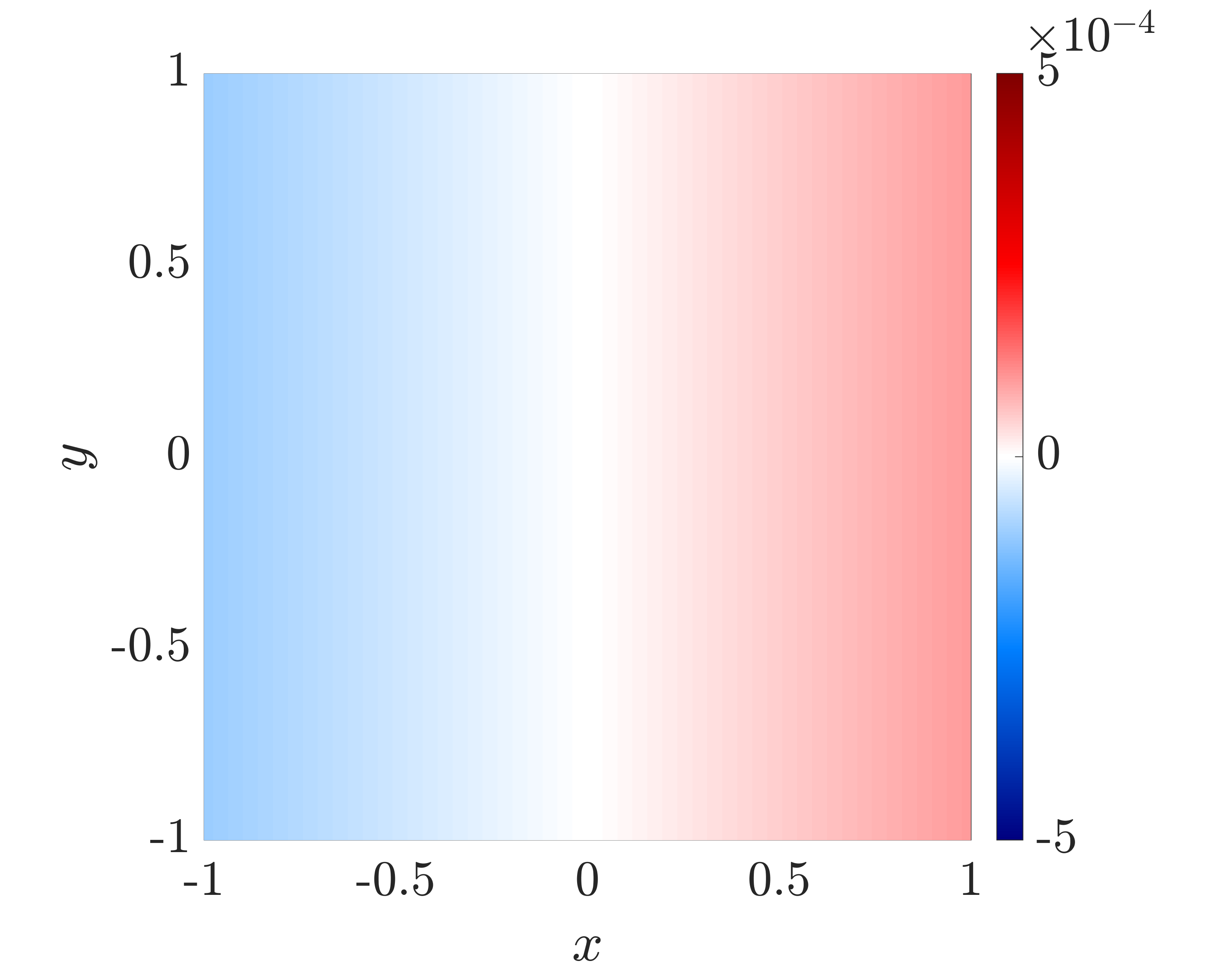
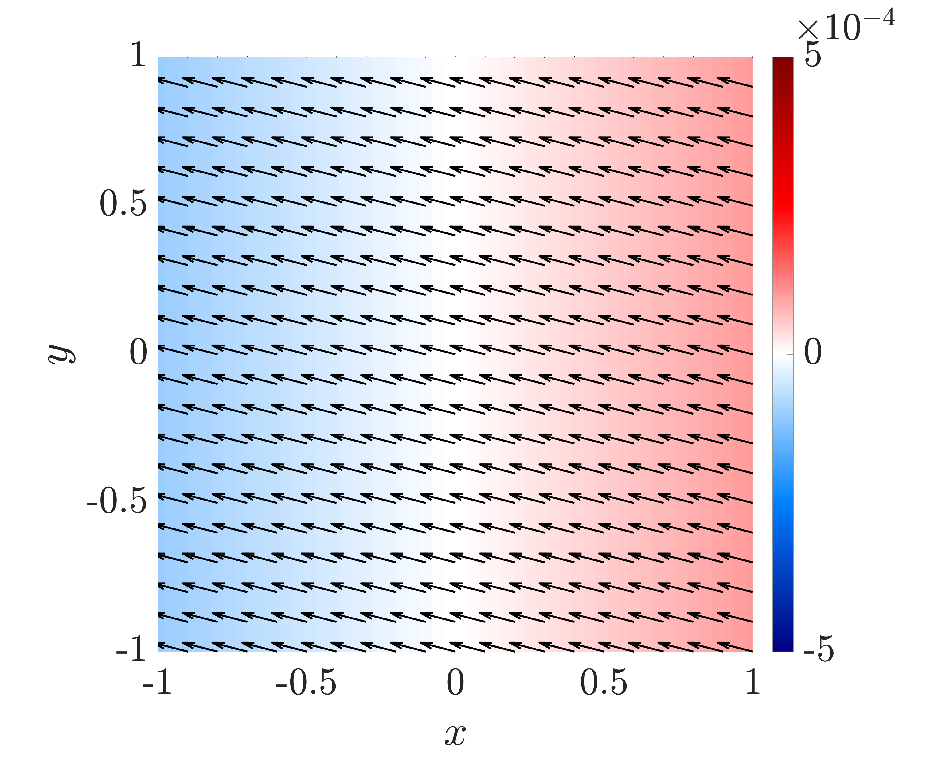
Figure 2: Velocity vector field $\boldsymbol{u}$ (arrow) and free surface height $h$ (contour) behaviour for Condition II: (a) initial condition at $t=0$ and (b) partial sum approximation based on ADM (with $N=6$) at $t=1$. Parameters used include $F=1$, $\bar{f}=0.5$, $D_{0}=0$, and $\eta_{x}=10^{-4}$ (Colour online).

(a)                                                                    (b)

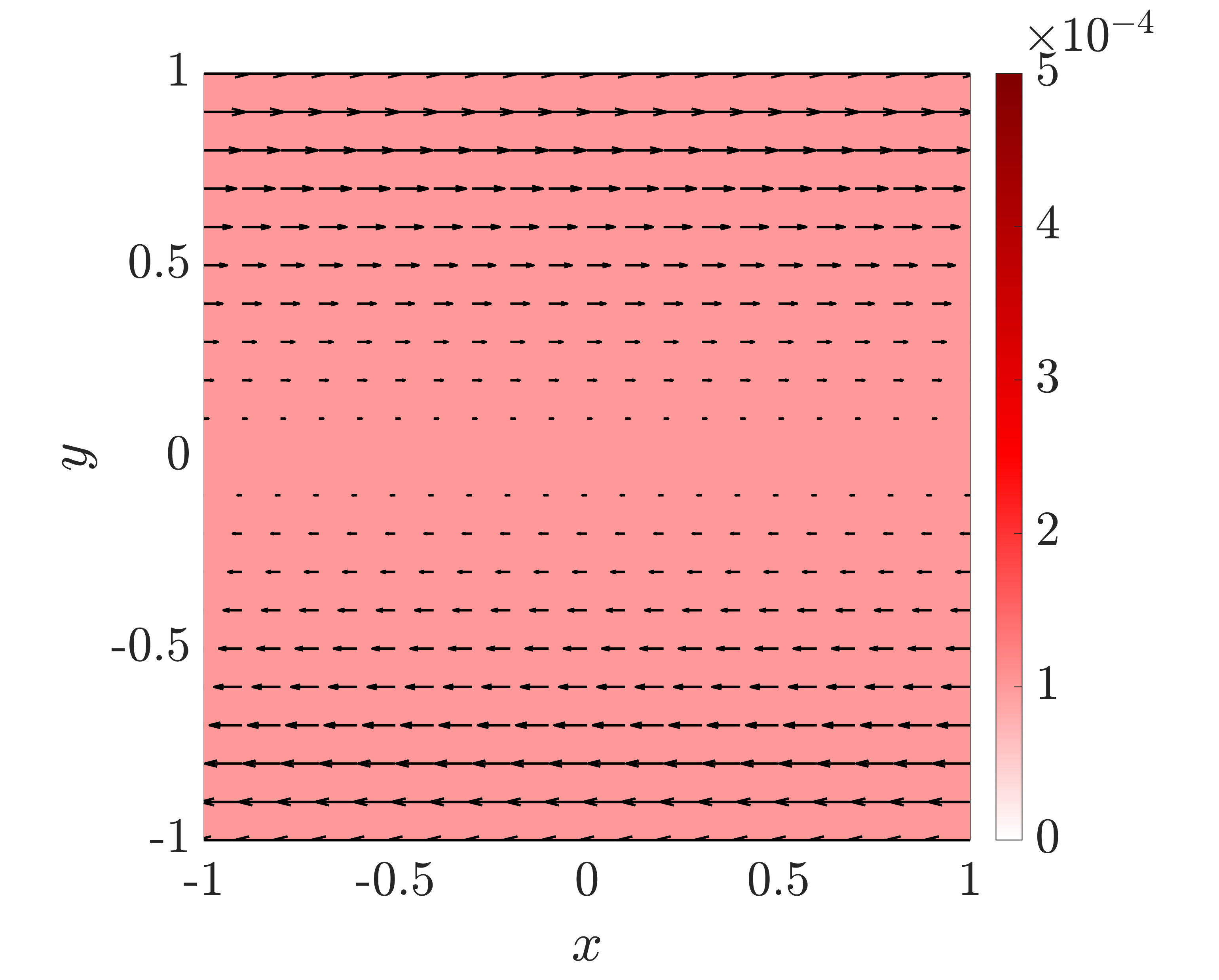
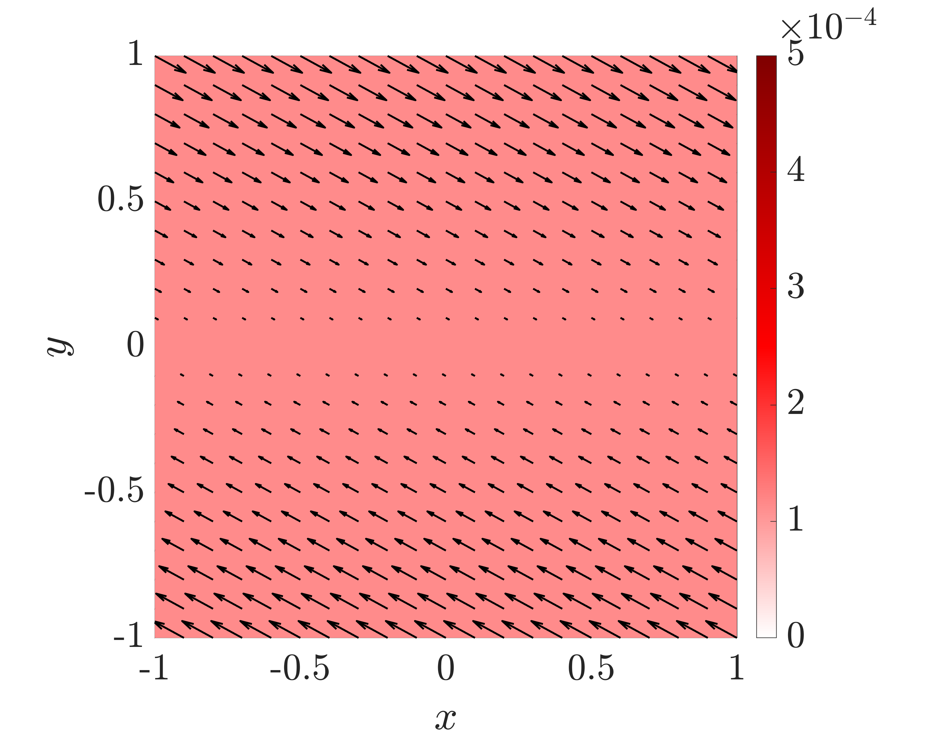
Figure 3: Velocity vector field $\boldsymbol{u}$ (arrow) and free surface height $h$ (contour) behaviour for Condition IV: (a) initial condition at $t=0$, (b) partial sum approximation based on ADM (with $N=6$) at $t=1$. Parameters used include $F=1$, $\bar{f}=0.5$, $D_{0}=0$, and $h_{0}=10^{-4}$ (Colour online).

5 Discussion

This work employs Adomian decomposition method (ADM) to the shallow water equations, where we made the following main contributions. First, we used these methods as reverse engineering mechanisms to develop theoretical connections between the ansatz formulations of previous works, such as Thacker (1981), Shapiro (1996) and Matskevich and Chubarov (2019), as well as develop a connection to the corresponding reduced systems of shallow water equations. Furthermore, we developed some novel families of closed-form solutions that respectively describe inertial oscillations and anticyclonic vortices with finite escape times over flat bottom topographies. We perform various numerical experiments against several cases that yielded relative errors between ${\rm O}\left(10^{-6}\right)$ and ${\rm O}\left(10^{-4}\right)$. Our numerical visualizations further demonstrate the validity of our approach, which illustrate the consistency with the dynamic behaviour for several scenarios while also preserving the correlation between the physical parameters.

Our study establishes the flexibility of these methods in terms of not only preserving the correlation of parameters with respect to the overall nonlinear physical behaviour but also alleviating the need to make restrictive assumptions like those based on the overall flow behaviour. Moreover, we illustrate that these techniques can be used to analytically deduce other aspects of shallow water phenomenon based on the characteristics of initial flows in which, to the best of our knowledge, this work is the first to explore these concepts. Therefore, some avenues of future work include extending these techniques to understand the implications of external forces such as the effects of bottom friction which are applicable to understanding various coastal effects such as impacts from tsunamis. Another area of research is extending this framework to analyse practical bottom topographies and shocks, which will consider bottom terrains that extend beyond those of parabolic shapes.

Disclosure statement

No potential conflict of interest was reported by the author(s).

Article Word Count

3,710 words

References

• Adomian (1990) Adomian, G., A review of the decomposition method and some recent results for nonlinear equations. Math. Comput. Modell., 1990, 13, 17–43.
• Adomian (2013) Adomian, G., Solving frontier problems of physics: the decomposition method, Vol. 60, 2013 (Springer Science & Business Media).
• Ball (1963) Ball, F.K., Some general theorems concerning the finite motion of a shallow rotating liquid lying on a paraboloid. J. Fluid Mech., 1963, 17, 240–256.
• Ball (1964) Ball, F.K., An exact theory of simple finite shallow water oscillations on a rotating earth; in Hydraul. Fluid Mech., 1964, pp. 293 – 305.
• Ball (1965) Ball, F.K., The effect of rotation on the simpler modes of motion of a liquid in an elliptic paraboloid. J. Fluid Mech., 1965, 22, 529–545.
• Bihlo et al. (2020) Bihlo, A., Poltavets, N. and Popovych, R.O., Lie symmetries of two-dimensional shallow water equations with variable bottom topography. Chaos, 2020, 30, 073132.
• Bila et al. (2006) Bila, N., Mansfield, E.L. and Clarkson, P.A., Symmetry group analysis of the shallow water and semi-geostrophic equations. Q. J. Mech. Appl. Math., 2006, 59, 95–123.
• Bollermann et al. (2011) Bollermann, A., Noelle, S. and Lukáčová-Medvid’ová, M., Finite volume evolution Galerkin methods for the shallow water equations with dry beds. Commun. Comput. Phys., 2011, 10, 371–404.
• Bristeau et al. (2021) Bristeau, M.O., Di Martino, B., Mangeney, A., Sainte-Marie, J. and Souillé, F., Some analytical solutions for validation of free surface flow computational codes. J. Fluid Mech., 2021, 913, A17.
• Chesnokov (2009) Chesnokov, A.A., Symmetries and exact solutions of the rotating shallow-water equations. Eur. J. Appl. Math., 2009, 20, 461–477.
• Chesnokov (2011) Chesnokov, A.A., Properties and exact solutions of the equations of motion of shallow water in a spinning paraboloid. J. Appl. Math. Mech., 2011, 75, 350–356.
• Clark and Herron (2013) Clark, A.D. and Herron, I.H., Improved bounds on linear instability of barotropic zonal flow within the shallow water equations. Geophys. Astrophys. Fluid Dyn., 2013, 107, 328–352.
• Clarkson and Kruskal (1989) Clarkson, P.A. and Kruskal, M.D., New similarity reductions of the Boussinesq equation. J. Math. Phys., 1989, 30, 2201–2213.
• Currò (1989) Currò, C., Some new exact solutions to the nonlinear shallow-water wave equations via group analysis. Meccanica, 1989, 24, 26–35.
• Cushman-Roisin (1987) Cushman-Roisin, B., Exact analytical solutions for elliptical vortices of the shallow-water equations. Tellus A, 1987, 39, 235–244.
• Cushman-Roisin et al. (1985) Cushman-Roisin, B., Heil, W.H. and Nof, D., Oscillations and rotations of elliptical warm-core rings. J. Geophys. Res.: Oceans, 1985, 90, 11756–11764.
• Delestre et al. (2013) Delestre, O., Lucas, C., Ksinant, P.A., Darboux, F., Laguerre, C., Vo, T.N.T., James, F. and Cordier, S., SWASHES: a compilation of shallow water analytic solutions for hydraulic and environmental studies. Int. J. Numer. Methods Fluids, 2013, 72, 269–300.
• Ern et al. (2008) Ern, A., Piperno, S. and Djadel, K., A well-balanced Runge–Kutta discontinuous Galerkin method for the shallow-water equations with flooding and drying. Int. J. Numer. Methods Fluids, 2008, 58, 1–25.
• Gallardo et al. (2007) Gallardo, J.M., Parés, C. and Castro, M., On a well-balanced high-order finite volume scheme for shallow water equations with topography and dry areas. J. Comput. Phys., 2007, 227, 574–601.
• Iacono (2005) Iacono, R., Analytic solutions to the shallow water equations. Phys. Rev. E, 2005, 72, 017302.
• Kafiabad et al. (2021) Kafiabad, H.A., Vanneste, J. and Young, W.R., Interaction of near-inertial waves with an anticyclonic vortex. J. Phys. Oceanogr., 2021, 51, 2035–2048.
• Kesserwani and Liang (2012) Kesserwani, G. and Liang, Q., Locally limited and fully conserved RKDG2 shallow water solutions with wetting and drying. J. Sci. Comput., 2012, 50, 120–144.
• Levi et al. (1989) Levi, D., Nucci, M., Rogers, C. and Winternitz, P., Group theoretical analysis of a rotating shallow liquid in a rigid container. J. Phys. A: Math. Gen., 1989, 22, 4743.
• Li et al. (2017) Li, M., Guyenne, P., Li, F. and Xu, L., A positivity-preserving well-balanced central discontinuous Galerkin method for the nonlinear shallow water equations. J. Sci. Comput., 2017, 71, 994–1034.
• Matskevich and Chubarov (2019) Matskevich, N.A. and Chubarov, L.B., Exact solutions to shallow water equations for a water oscillation problem in an idealized basin and their use in verifying some numerical algorithms. Numer. Anal. Appl., 2019, 12, 234–250.
• McKiver (2020) McKiver, W.J., Balanced ellipsoidal vortex at finite Rossby number. Geophys. Astrophys. Fluid Dyn., 2020, 114, 453–480.
• Meleshko (2020) Meleshko, S.V., Complete group classification of the two-dimensional shallow water equations with constant Coriolis parameter in Lagrangian coordinates. Commun. Nonlinear Sci. Numer. Simul., 2020, 89, 105293.
• Meleshko and Samatova (2020) Meleshko, S.V. and Samatova, N.F., Group classification of the two-dimensional shallow water equations with the beta-plane approximation of Coriolis parameter in Lagrangian coordinates. Commun. Nonlinear Sci. Numer. Simul., 2020, 90, 105337.
• Nikolos and Delis (2009) Nikolos, I.K. and Delis, A.I., An unstructured node-centered finite volume scheme for shallow water flows with wet/dry fronts over complex topography. Comput. Methods Appl. Mech. Eng., 2009, 198, 3723–3750.
• Pedlosky (2013) Pedlosky, J., Geophysical fluid dynamics, 2013 (Springer Science & Business Media).
• Rogers (1989a) Rogers, C., Generation of invariance theorems for nonlinear boundary-value problems in shallow water theory: an application of MACSYMAa; in Numerical and Applied Mathematics, IMACS Meeting Proceedings, Paris, 1989a, pp. 69–74.
• Rogers (1989b) Rogers, C., Elliptic warm-core theory: The pulsrodon. Phys. Lett. A, 1989b, 138, 267–273.
• Sachdev et al. (1996) Sachdev, P.L., Palaniappan, D. and Sarathy, R., Regular and chaotic flows in paraboloidal basins and eddies. Chaos, Solitons Fractals, 1996, 7, 383–408.
• Sampson et al. (2005) Sampson, J., Easton, A. and Singh, M., Moving boundary shallow water flow above parabolic bottom topography. ANZIAM J., 2005, 47, 373–387.
• Shapiro (1996) Shapiro, A., Nonlinear shallow-water oscillations in a parabolic channel: exact solutions and trajectory analyses. J. Fluid Mech., 1996, 318, 49–76.
• Sun (2016) Sun, C., High-order exact solutions for pseudo-plane ideal flows. Phys. Fluids, 2016, 28, 083602.
• Thacker (1977) Thacker, W.C., Irregular grid finite-difference techniques: simulations of oscillations in shallow circular basins. J. Phys. Oceanogr., 1977, 7, 284–292.
• Thacker (1981) Thacker, W.C., Some exact solutions to the nonlinear shallow-water wave equations. J. Fluid Mech., 1981, 107, 499–508.
• Tsang and Dritschel (2015) Tsang, Y.K. and Dritschel, D.G., Ellipsoidal vortices in rotating stratified fluids: beyond the quasi-geostrophic approximation. J. Fluid Mech., 2015, 762, 196–231.
• Vallis (2017) Vallis, G.K., Atmospheric and oceanic fluid dynamics, 2017 (Cambridge University Press).
• Vallis (2019) Vallis, G.K., Essentials of Atmospheric and Oceanic Dynamics, 2019 (Cambridge University Press).
• Wintermeyer et al. (2018) Wintermeyer, N., Winters, A.R., Gassner, G.J. and Warburton, T., An entropy stable discontinuous Galerkin method for the shallow water equations on curvilinear meshes with wet/dry fronts accelerated by GPUs. J. Comput. Phys., 2018, 375, 447–480.