Assigning Agents to Increase Network-Based
Neighborhood Diversity

Abstract

Motivated by real-world applications such as the allocation of public housing, we examine the problem of assigning a group of agents to vertices (e.g., spatial locations) of a network so that the diversity level is maximized. Specifically, agents are of two types (characterized by features), and we measure diversity by the number of agents who have at least one neighbor of a different type. This problem is known to be NP-hard, and we focus on developing approximation algorithms with provable performance guarantees. We first present a local-improvement algorithm for general graphs that provides an approximation factor of $1/2$. For the special case where the sizes of agent subgroups are similar, we present a randomized approach based on semidefinite programming that yields an approximation factor better than $1/2$. Further, we show that the problem can be solved efficiently when the underlying graph is treewidth-bounded and obtain a polynomial time approximation scheme (PTAS) for the problem on planar graphs. Lastly, we conduct experiments to evaluate the performance of the proposed algorithms on synthetic and real-world networks.

Conference version. The conference version of the paper is accepted at AAMAS-2023: link.

1 Introduction

Many countries have public housing initiatives that offer low-income individuals secure and affordable residences. Housing options are typically allocated by government agencies that involve a process of assigning applicants to vacant apartments [39, 14]. Given that the applicants often come from a variety of demographic groups, the spatial distribution of public housing partially shapes the demographic structure of local communities [35, 16]. The promotion and cultivation of integrated communities is an objective of contemporary societies. It has been shown that integration can improve a country’s financial performance, reduce the disparity between demographic groups, and advance social prosperity in general [9, 24, 36]. Conversely, segregated neighborhoods widen the socioeconomic divide in the population. As noted by many social scientists, residential segregation remains a persistent problem that directly contributes to the uneven distribution of resources and limited life chances for some groups (e.g., [33, 38, 40]).

In this work, we study the problem of promoting community integration (i.e., diversity) in the context of housing assignment. Indeed, public housing programs often take diversity into account. In Singapore, there are established policies to ensure that a certain ethnic quota must be satisfied for each project at the neighborhood level [10]. In the U.S., cities like Chicago and New York also place emphasis on the value of having integrated communities [29, 8]. Nevertheless, formal computational methods for improving the level of integration in the housing assignment process have received limited attention. Motivated by the above considerations, we investigate the problem of public housing allocation from an algorithmic perspective and provide systematic approaches to design assignment strategies that enhance community integration.

Formally, we model a housing project as a graph $\mathcal{G}{}=(\mathcal{V}{},\mathcal{E}{})$ where $\mathcal{V}{}$ is the set of vacant residences, and the edges in $\mathcal{E}{}$ represent proximity between residences. We are also given a set $\mathcal{A}$ of agents representing the applicants to be assigned to residences. Agents are partitioned into two demographic subgroups: type-1 and type-2. Without loss of generality, we assume that the number of type-1 agents does not exceed the number of type-2 agents. (We sometimes use the phrase “minority agents” for type-1 agents.) We also assume that the number of vacant residences (i.e., $|\mathcal{V}|$) equals the number of agents. Our goal is to construct an assignment (bijective mapping) $\mathcal{P}$ of residences to agents that maximizes the the integration level of the layout of agents on $\mathcal{G}{}$.

To quantify the integration level of a given assignment $\mathcal{P}$, we use the index of integration (IoA) metric proposed in [1]. This index is defined as the number of integrated agents, that is, agents with at least one neighbor of a different type in $\mathcal{G}{}$. An illustrative example is given in Fig. 1. We refer to the above assignment problem as Integration Maximization - Index of Agent Integration (IM-IoA). We note that this problem could also arise in other settings where integration is preferred, such as dormitory assignments for freshmen in universities [6].

The problem of maximizing IoA is known to be NP-hard [1]. Nevertheless, the authors of [1] did not address approximation questions for the problem, as their focus is on game theoretic aspects of IoA. In this work, we focus on developing approximation algorithms with provable performance guarantees for IM-IoA. Our main contributions are as follows.

• Approximation for general instances. We present a local-improvement algorithm that guarantees a factor $1/2$ approximation. We further show that our analysis is tight by presenting an example that achieves this bound. While it is possible to derive an approximation for the problem using a general result in [7], the resulting performance guarantee is $0.356$, which is weaker than our factor of $1/2$.

• Improved approximation for special instances. For the case when the number of type-1 agents is a constant fraction $\alpha$ of the total number of agents, $0<\alpha\leq 1/2$, we present a semidefinite programming (SDP) based randomized algorithm that yields approximation ratios in the range $[0.516,0.649]$ for $\alpha$ in the range $[0.403,0.5]$. For example, when $\alpha=0.45$, the ratio is $0.578$, and when $\alpha=0.5$, the ratio is $0.649$.

• A polynomial time approximation scheme for planar graphs. We present a dynamic programming algorithm that solves IM-IoA in polynomial time on graphs with bounded treewidth. Using this result in conjunction with a technique due to Baker [2], we obtain a polynomial time approximation scheme (PTAS) for the problem on planar graphs. For any fixed $\epsilon>0$, the algorithm provides a performance guarantee of $1-\epsilon$.

• Empirical analysis. We study the empirical performance of the proposed local-improvement algorithm against baseline methods on both synthetic and real-world networks. Overall, we observe that the empirical approximation ratio of the proposed algorithm is much higher than $1/2$, which is our theoretical guarantee.

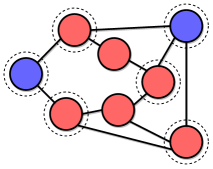
Figure 1: An example assignment of two type-1 agents (blue) and six type-2 agents (red) on a graph $\mathcal{G}{}$. Vertices with integrated agents are labeled by dashed circles. The index of integration for this assignment (ie., the number of integrated agents) is $6$.

2 Related Work

Integration in public housing.

Issues regarding segregation and the need for enhancing integration have been documented extensively in the social science literature (e.g., [12, 25, 22, 27]). In particular, many works on segregation in social networks (e.g., [17, 19]) stem from the pioneering models proposed by Schelling [34], where agents move between vertices to improve their utility values. While Schelling’s framework allows the study of agent dynamics, Benabbou et al. [4] study integration in public housing allocation from a planning perspective. In particular, they formulate the setting as a weighted matching problem where the set of available houses is partitioned into blocks, and agents are assigned (by some central agency) to blocks to maximize a utility measure while satisfying some diversity constraints. They establish the NP-hardness of the problem and present an approximation algorithm based on a result of Stamoulis [37]. A number of other studies have also addressed integration in the context of public housing from a social science perspective (e.g., [31, 20, 23, 18]).

The problem formulations and the algorithmic techniques used in Benabbou et al. [4] and in our work are significantly different. First, Benabbou et al. [4] examine a weighted matching problem. Their model does not use any network structure for the residences, whereas our work approaches the problem from a graph theoretic standpoint, with the underlying network playing an important role in the formulation. Further, the integration index studied in our work is defined w.r.t graph structures, whereas the measure used in [4] is based on constraints on the ethnicity quotas for blocks. More importantly, the goal of our work is to find an assignment that maximizes the integration level, whereas the goal in [4] is to maximize the overall utility of agents under a diversity constraint.

Integration indices.

Various indices to measure the level of integration in a population are surveyed in [25]. However, most of those indices cannot be naturally extended to a network setting. The integration index IoA considered in our work was proposed by Agarwal et al. [1] in the context of the Schelling Game on networks, where agents can change locations to increase their utilities. Agarwal et al. explore several properties (e.g., the integration price of anarchy/stability) of the index from a game theoretic perspective. Further, they show that finding an assignment for which all agents are integrated (i.e., each agent has at least one neighbor of a different type) is NP-hard [1].

Approximation algorithms.

Our approximation algorithm for general IM-IoA is based on a local-improvement scheme. A well-known problem for which a local-improvement algorithm provides an approximation guarantee of 1/2 is the unweighted MaxCut problem [26]. We note that the analysis used to establish the performance guarantees of the local-improvement methods for MaxCut and IM-IoA are substantially different. In particular, MaxCut has no cardinality constraints, and the objective is defined w.r.t edges. In contrast, IM-IoA requires that a specified number of vertices be assigned to type-1 agents, and the objective is defined w.r.t vertices. One can also formulate IM-IoA as a non-monotone submodular function maximization problem. Since such a formulation requires a strict equality constraint (involving type-1 agents), the best known performance guarantee under the general non-monotone submodular maximization framework with such a constraint is $0.356$ [7].

3 Problem Definition

We study the problem of assigning vertices in a graph to a group of agents, such that the integration level of the resulting layout of agents in the graph is maximized. We begin with key notations and then define the integration maximization problem formally.

Graphs and agents.

Let $\mathcal{G}{}=(\mathcal{V}{},\mathcal{E}{})$ be an undirected graph, where $\mathcal{V}{}$ is a set of vertices representing vacant residences, and $\mathcal{E}{}$ is a set of edges representing the proximity relationship between residences. Let $\mathcal{A}{}$ be the set of agents to be assigned to $\mathcal{V}{}$. The set of agents is divided into two demographic subgroups. Formally, $\mathcal{A}$ is partitioned into two subsets $\mathcal{A}{}_{1}$ and $\mathcal{A}{}_{2}$; we refer to agents in $\mathcal{A}{}_{i}$ as type $i$ agents, $i=\texttt{1},\texttt{2}$. Let $k=|\mathcal{A}{}_{\texttt{1}}|$ denote the number of type-1 agents, so $n-k$ is the number of type-2 agents. Without loss of generality, let $k\leq n/2$, and we refer to $\mathcal{A}{}_{\texttt{1}}$ as the minority subgroup. Lastly, we assume that $|\mathcal{V}{}|=|\mathcal{A}|$; that is, the number of vertices is the same as the number of agents.

Assignment.

An assignment is a mapping from vertices to agents. To simplify the proofs, we use an equivalent definition where an assignment is a mapping from vertices to agent types. In particular, an assignment $\mathcal{P}:\mathcal{V}{}\rightarrow\{\texttt{1},\texttt{2}\}$ is a function that assigns an agent type to each vertex in $\mathcal{V}$, such that $k$ vertices are assigned type-1 and $n-k$ vertices are assigned type-2. In such an assignment, a type-$i$ vertex is occupied by a type-$i$ agent, $i=\texttt{1},\texttt{2}$. We remark that the above definition of an assignment is mathematically equivalent to defining an assignment to be a mapping from $\mathcal{V}{}$ to $\mathcal{A}{}$.

The index of integration.

We consider the integration index proposed in [1] and apply it to our context.

Definition 3.1 (Index of agent-integration (IoA) [1]).

Given an assignment $\mathcal{P}$, an agent $x\in\mathcal{A}$ is integrated if $x$ has at least one neighbor in $\mathcal{G}{}$ whose type is different from that of $x$. Let $\mathcal{A}^{\prime}$ be the set of integrated agents under $\mathcal{P}$. The index of agent-integration of $\mathcal{P}$ is then defined as the number of integrated agents in $\mathcal{A}$:

$$\texttt{IoA}(\mathcal{P})=|\mathcal{A}^{\prime}|$$ (1)

Equivalently, a vertex $u\in\mathcal{V}{}$ is integrated under $\mathcal{P}$ if the agent assigned to $u$ is integrated. Thus, we may also view the index as $\texttt{IoA}(\mathcal{P})=|\mathcal{V}^{\prime}|$ where $\mathcal{V}{}^{\prime}$ is the set of integrated vertices under $\mathcal{P}$. These two definitions of IoA are mathematically equivalent.

The optimization problem.

We now define the problem IM-IoA.

Definition 3.2 (IM-IoA).

Given a graph $\mathcal{G}{}=(\mathcal{V}{},\mathcal{E}{})$, a set $\mathcal{A}$ of agents with $k$ type-1 and $n-k$ type-2 agents, find an assignment $\mathcal{P}$ such that $\texttt{IoA}(\mathcal{P})$ is maximized.

We note that IM-IoA can be viewed as an optimization version of 2-weak coloring [28], where the number of vertices with each color is specified, and the number of properly colored vertices is maximized.

4 Approximation for General Graphs

IM-IoA is NP-hard, as established in [1]. In this section, we present a local-improvement algorithm for IM-IoA and show that the algorithm achieves a factor $1/2$ approximation for general graphs. For convenience in presenting the proofs, we consider an assignment from the perspective of vertices rather than that of the agents. As stated earlier, these two definitions are equivalent.

The algorithm.

We start from a random assignment $\mathcal{P}$. In each iteration of the algorithm, we find (if possible) a pair of type-1 and type-2 vertices such that swapping their types strictly increases the objective. In particular, let $u$ be a type-1 vertex, and $v$ be a type-2 vertex. We swap the types of $u$ and $v$ (i.e., $u$ becomes type-2 and $v$ becomes type-1) if and only if the resulting new assignment $\mathcal{P}^{\prime}$ has a strictly higher IoA; that is, $\texttt{IoA}(\mathcal{P})<\texttt{IoA}(\mathcal{P}^{\prime})$. The algorithm terminates when no such swap can be made. The pseudocode is given in Algorithm (1).

1

Input : A graph $\mathcal{G}{}=(\mathcal{V}{},\mathcal{E}{})$, $k$, where $k\leq|\mathcal{V}{}|/2$

Output : An assignment $\mathcal{P}$

2

3$\mathcal{P}\leftarrow$ a random assignment & $\texttt{Updated}\leftarrow\text{True}$

4while Updated do

5       $\texttt{Updated}\leftarrow\text{False}$

6      for $x\in\mathcal{V}{}_{1}(\mathcal{P})$ do

7             for $y\in\mathcal{V}{}_{2}(\mathcal{P})$ do

8                   $\mathcal{P}^{\prime}\leftarrow$ the assignment where $\mathcal{P}^{\prime}(x)=\mathcal{P}(y)$ and $\mathcal{P}^{\prime}(y)=\mathcal{P}(x)$

9                  if $\texttt{IoA}(\mathcal{P}^{\prime})>\texttt{IoA}(\mathcal{P})$ then

10                         $\mathcal{P}=\mathcal{P}^{\prime}$, $\texttt{Updated}\leftarrow\text{True}$ & break

11                  

12            

13      

return $\mathcal{P}$

Algorithm 1 Local-Improvement-IoA

4.1 Analysis of the algorithm

Given a problem instance of IM-IoA, let $\mathcal{P}$ be a saturated assignment returned by Algorithm (1). Let $\mathcal{P}^{*}$ be an optimal assignment that achieves the maximum objective, denoted by OPT. We assume that $\mathcal{P}\neq\mathcal{P}^{*}$. In this section, we show that $\texttt{IoA}(\mathcal{P})\geq 1/2\cdot\texttt{IoA}(\mathcal{P}^{*})=1/2\cdot\textsc{OPT}$, thereby establishing a $1/2$ approximation. Due to the page limit, we sketch the proof here; the full proof appears in the appendix.

Given an assignment $\mathcal{P}$, which is a mapping from vertices to agent types, we call a vertex $v$ a type-1 (or type-2) vertex if $\mathcal{P}(v)=1$ (or $\mathcal{P}(v)=2$). Let $\mathcal{V}{}_{1}(\mathcal{P})$ and $\mathcal{V}{}_{2}(\mathcal{P})$ denote the set of type-1 and type-2 vertices under $\mathcal{P}$. Let $\mathcal{V}^{\texttt{U}}_{1}(\mathcal{P})$ and $\mathcal{V}^{\texttt{U}}_{2}(\mathcal{P})$ denote the set of uncovered type-1 and type-2 vertices under $\mathcal{P}$. For each vertex $u$, let $\mathcal{N}^{\texttt{U}}_{u}(\mathcal{P})$ denote the set of neighbors of $u$ that are uncovered under $\mathcal{P}$, and let $\Gamma_{u}(\mathcal{P})$ denote the set of different-type neighbors of $u$ that are uniquely covered by $u$, i.e., $\Gamma_{u}(\mathcal{P})$ is the set of vertices $v$ such that $(i)$ $v$ is a neighbor of $u$, $(ii)$ the type of $v$ is different from the type of $u$, and $(iii)$ $v$ has no other neighbor whose type is the same as $u$’s type.

Observation 4.1.

The index $\texttt{IoA}(\mathcal{P})=n-|\mathcal{V}^{\texttt{U}}_{1}(\mathcal{P})|-|\mathcal{V}^{\texttt{U}}_{2}(\mathcal{P})|$.

We now consider the following mutually exclusive and collectively exhaustive cases of $\mathcal{V}^{\texttt{U}}_{1}(\mathcal{P})$ and $\mathcal{V}^{\texttt{U}}_{2}(\mathcal{P})$ under the saturated assignment $\mathcal{P}$. We start with a simple case where all the type-2 vertices under $\mathcal{P}$ are integrated.

Case 1: $\mathcal{V}^{\texttt{U}}_{2}(\mathcal{P})=\emptyset$.

Under this case, all vertices in $\mathcal{V}{}_{2}(\mathcal{P})$ are integrated which gives

$$\texttt{IoA}(\mathcal{P})\geq|\mathcal{V}^{\texttt{U}}_{2}(\mathcal{P})|=n-k\geq\frac{1}{2}\cdot n\geq\frac{1}{2}\cdot\textsc{OPT}$$ (2)

The above case trivially implies that the algorithm provides a $1/2$ approximation. We now look at the remaining case where $\mathcal{V}^{\texttt{U}}_{2}(\mathcal{P})\neq\emptyset$.

Case 2: $\mathcal{V}^{\texttt{U}}_{2}(\mathcal{P})\neq\emptyset$.

Under this case, there exists at least one vertex in $\mathcal{V}{}_{2}(\mathcal{P})$ that is not integrated. We first show that $\mathcal{V}^{\texttt{U}}_{1}(\mathcal{P})$ and $\mathcal{V}^{\texttt{U}}_{2}(\mathcal{P})$ cannot both be non-empty.

Lemma 4.2.

For a saturated assignment $\mathcal{P}$, if $\mathcal{V}^{\texttt{U}}_{2}(\mathcal{P})\neq\emptyset$, then $\mathcal{V}^{\texttt{U}}_{1}(\mathcal{P})=\emptyset$.

Proof.

(Sketch) Let $y\in\mathcal{V}^{\texttt{U}}_{2}(\mathcal{P})$ be a vertex of type-2 that is not integrated (i.e., all neighbors of $y$ are of type-2). For contradiction, suppose $\mathcal{V}^{\texttt{U}}_{1}(\mathcal{P})\neq\emptyset$. Now let $x\in\mathcal{V}^{\texttt{U}}_{1}(\mathcal{P})$ be an non-integrated vertex of type-1 whose neighbors are all of type-1. Let $\mathcal{P}^{\prime}$ denote the assignment where we switch the types between $x$ and $y$, that is, $\mathcal{P}^{\prime}(x)=\mathcal{P}(y)=\texttt{2}$, $\mathcal{P}^{\prime}(y)=\mathcal{P}(x)=\texttt{1}$, while the types of all other vertices remain unchanged. One can verify that $\texttt{IoA}(\mathcal{P}^{\prime})\geq\texttt{IoA}(\mathcal{P})+2$, that is, switching the types of $x$ and $y$ increases the index IoA by at least $2$. This implies the existence of an improvement move from $\mathcal{P}$, which contradicts the fact that $\mathcal{P}$ is saturated. It follows that $\mathcal{V}^{\texttt{U}}_{1}(\mathcal{P})=\emptyset$. ∎

Lemma (4.2) implies that under case 2 (i.e., $\mathcal{V}^{\texttt{U}}_{2}(\mathcal{P})\neq\emptyset$), we have $\mathcal{V}^{\texttt{U}}_{1}(\mathcal{P})=\emptyset$. We now consider the following two mutually exclusive and collectively exhaustive subcases under Case $2$ and show that the approximation factor under each subcase is $1/2$.

Subcase 2.1: $\mathcal{V}^{\texttt{U}}_{2}(\mathcal{P})\neq\emptyset$, and $\Gamma_{x}(\mathcal{P})\neq\emptyset,\;\;\forall x\in\mathcal{V}{}_{1}(\mathcal{P})$, that is, for each type-1 vertex $x\in\mathcal{V}{}_{1}(\mathcal{P})$, there is at least one type-2 neighbor of $x$ that is uniquely covered by $x$.

Suppose $\mathcal{P}\neq\mathcal{P}^{*}$, namely, for some $x\in\mathcal{V}{}$, $\mathcal{P}(x)\neq\mathcal{P}^{*}(x)$. Let $\tilde{\mathcal{V}{}}_{2-1}=\{v\in\mathcal{V}{}\;:\;\mathcal{P}(v)=2,\mathcal{P}^{*}(v)=1\}$ be the set of vertices that are type-2 under $\mathcal{P}$, but are type-1 under $\mathcal{P}^{*}$. Analogously, let $\tilde{\mathcal{V}{}}_{1-2}=\{v\in\mathcal{V}{}\;:\;\mathcal{P}(v)=1,\mathcal{P}^{*}(v)=2\}$ be the set of vertices of type-1 under $\mathcal{P}$, but are of type-2 under $\mathcal{P}^{*}$. Observe that $|\tilde{\mathcal{V}{}}_{2-1}|=|\tilde{\mathcal{V}{}}_{1-2}|$. One may view $\mathcal{P}^{*}$ as the result of a transformation from $\mathcal{P}$ under pairwise swaps of types between $\tilde{\mathcal{V}{}}_{2-1}$ and $\tilde{\mathcal{V}{}}_{1-2}$. An example is given in Figure (2). We present a key lemma that bounds the difference between the objective values of $\mathcal{P}$ and $\mathcal{P}^{*}$.

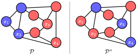
Figure 2: Two assignments $\mathcal{P}$ and $\mathcal{P}^{*}$ where type-1 and type-2 vertices are highlighted in blue and red, respectively. In this case, $\tilde{\mathcal{V}{}}_{2-1}=\{x_{3},x_{4}\}$ and $\tilde{\mathcal{V}{}}_{1-2}=\{x_{1},x_{2}\}$. We may then transform $\mathcal{P}$ into $\mathcal{P}^{*}$ by swapping types between the pair $(x_{1},x_{3})$ and between $(x_{2},x_{4})$. Note that this example is only to demonstrate how $\tilde{\mathcal{V}{}}_{2-1}$ and $\tilde{\mathcal{V}{}}_{1-2}$ are defined, as $\mathcal{P}$ cannot be a saturated assignment returned by the algorithm.

Lemma 4.3 (Subcase 2.1).

Let $\mathcal{P}$ be a saturated assignment under subcase 2.1, and let $\mathcal{P}^{*}$ be an optimal assignment. We have

$$\texttt{IoA}(\mathcal{P}^{*})-\texttt{IoA}(\mathcal{P}) \leq\sum_{y\in\tilde{\mathcal{V}{}}_{2-1}\setminus\mathcal{V}^{\texttt{U}}_{2}(\mathcal{P})}|(\mathcal{N}(y)\cap\mathcal{V}^{\texttt{U}}_{2}(\mathcal{P})|$$ (3)

$$+\sum_{y\in\tilde{\mathcal{V}{}}_{2-1}\cap\mathcal{V}^{\texttt{U}}_{2}(\mathcal{P})}\left(|(\mathcal{N}(y)\cap\mathcal{V}^{\texttt{U}}_{2}(\mathcal{P})|+1\right).$$

Proof.

(Sketch) Since $\mathcal{P}$ is saturated, Lemma (4.2) implies that all type-1 vertices under $\mathcal{P}$ are integrated. Thus, the difference $\texttt{IoA}(\mathcal{P}^{*})-\texttt{IoA}(\mathcal{P})$ is at most the number of type-2 vertices that are integrated under $\mathcal{P}^{*}$ but are not integrated under $\mathcal{P}$.

Let $f:\tilde{\mathcal{V}{}}_{1-2}\rightarrow\tilde{\mathcal{V}{}}_{2-1}$ be an arbitrary bijective mapping. We may regard $\mathcal{P}^{*}$ as a result of the transformation from $\mathcal{P}$ via pairwise swaps of types between vertices specified by $f$ (i.e., the type of $x\in\tilde{\mathcal{V}{}}_{1-2}$ is swapped with the type of $f(x)\in\tilde{\mathcal{V}{}}_{2-1}$). Observe that only vertices in $\mathcal{V}^{\texttt{U}}_{2}(\mathcal{P})$ that are adjacent to $\tilde{\mathcal{V}{}}_{2-1}$ (or within $\tilde{\mathcal{V}{}}_{2-1}$) under $\mathcal{P}$ can be newly integrated under $\mathcal{P}^{*}$ after swapping $\tilde{\mathcal{V}{}}_{1-2}$ with $\tilde{\mathcal{V}{}}_{2-1}$ (by the definition of $\mathcal{V}^{\texttt{U}}_{2}(\mathcal{P})$, vertices in $\tilde{\mathcal{V}{}}_{1-2}$ have no neighbors in $\mathcal{V}^{\texttt{U}}_{2}(\mathcal{P})$.). It follows that for each vertex $y\in\tilde{\mathcal{V}{}}_{2-1}$, at most $|(\mathcal{N}(y)\cap\mathcal{V}^{\texttt{U}}_{2}(\mathcal{P})|$ of its neighbors can become newly integrated after transforming from $\mathcal{P}$ to $\mathcal{P}^{*}$. Further, if also $y\in\tilde{\mathcal{V}{}}_{2-1}\cap\mathcal{V}^{\texttt{U}}_{2}(\mathcal{P})$, $y$ itself could also be newly integrated after the swap. We then have

$$\texttt{IoA}(\mathcal{P}^{*})-\texttt{IoA}(\mathcal{P}) \leq|\bigcup_{y\in\tilde{\mathcal{V}{}}_{2-1}}\mathcal{N}(y)\cap\mathcal{V}^{\texttt{U}}_{2}(\mathcal{P})|+|\tilde{\mathcal{V}{}}_{2-1}\cap\mathcal{V}^{\texttt{U}}_{2}(\mathcal{P})|$$

$$\leq\sum_{y\in\tilde{\mathcal{V}{}}_{2-1}\setminus\mathcal{V}^{\texttt{U}}_{2}(\mathcal{P})}|(\mathcal{N}(y)\cap\mathcal{V}^{\texttt{U}}_{2}(\mathcal{P})|$$ (4)

$$+\sum_{y\in\tilde{\mathcal{V}{}}_{2-1}\cap\mathcal{V}^{\texttt{U}}_{2}(\mathcal{P})}\left(|(\mathcal{N}(y)\cap\mathcal{V}^{\texttt{U}}_{2}(\mathcal{P})|+1\right)$$

where the last inequality follows from the union bound. ∎

We now proceed to show that the difference between $\texttt{IoA}(\mathcal{P}^{*}$ and $\texttt{IoA}(\mathcal{P})$ established in Lemma (4.3) is at most $\texttt{IoA}(\mathcal{P})$, thereby establishing $\texttt{IoA}(\mathcal{P})\geq\frac{1}{2}\cdot\texttt{IoA}(\mathcal{P}^{*})$. Recall that for each vertex $x\in\mathcal{V}{}$, $\Gamma_{x}(\mathcal{P})$ is the set of neighbors of $x$ whose types are different from $x$, and are uniquely covered by $x$ under $\mathcal{P}$. By the definition of Subcase $2.1$, $\Gamma_{x}(\mathcal{P})$ is not empty for all $x\in\mathcal{V}{}_{1}(\mathcal{P})$. We first argue that for any $y\in\mathcal{V}^{\texttt{U}}_{2}(\mathcal{P})$ and any $x\in\mathcal{V}{}_{1}(\mathcal{P})$, we have $|\mathcal{N}(y)\cap\mathcal{V}^{\texttt{U}}_{2}(\mathcal{P})|\leq|\Gamma_{x}(\mathcal{P})|$.

Lemma 4.4 (Subcase 2.1).

Given a saturated assignment $\mathcal{P}$, for any $y\in\mathcal{V}^{\texttt{U}}_{2}(\mathcal{P})$ and any $x\in\mathcal{V}{}_{1}(\mathcal{P})$, we have

$$|\mathcal{N}(y)\cap\mathcal{V}^{\texttt{U}}_{2}(\mathcal{P})|\leq|\Gamma_{x}(\mathcal{P})|.$$

Proof.

(Sketch) Given that $y$ is not integrated under $\mathcal{P}$, $x$ and $y$ cannot be adjacent. Since $\mathcal{P}$ is a saturated assignment, if the types of $x$ and $y$ are to be swapped, the number of newly integrated vertices would be at most the number of newly non-integrated vertices. Further, one can verify that the number of vertices that are newly integrated is at least $|\mathcal{N}(y)\cap\mathcal{V}^{\texttt{U}}_{2}(\mathcal{P})|+1$, and the number of vertices that are newly non-integrated is at most $|\Gamma_{x}(\mathcal{P})|+1$. Since $\mathcal{P}$ is saturated, it follows that $|\mathcal{N}(y)\cap\mathcal{V}^{\texttt{U}}_{2}(\mathcal{P})|\leq|\Gamma_{x}(\mathcal{P})|$. This concludes the proof. ∎

We now establish the next Lemma, which bounds the size of $\mathcal{N}(y)\cap\mathcal{V}^{\texttt{U}}_{2}(\mathcal{P})$ for $y\in\mathcal{V}{}_{2}(\mathcal{P})\setminus\mathcal{V}^{\texttt{U}}_{2}(\mathcal{P})$ and $x\in\mathcal{V}{}_{1}(\mathcal{P})$.

Lemma 4.5 (Subcase 2.1).

Given a saturated assignment $\mathcal{P}$, for any $y\in\mathcal{V}{}_{2}(\mathcal{P})\setminus\mathcal{V}^{\texttt{U}}_{2}(\mathcal{P})$ and any $x\in\mathcal{V}{}_{1}(\mathcal{P})$, we have

$$|\mathcal{N}(y)\cap\mathcal{V}^{\texttt{U}}_{2}(\mathcal{P})|\leq|\Gamma_{x}(\mathcal{P})|+1$$

Proof.

(Sketch) We partition $\mathcal{V}{}_{2}(\mathcal{P})\setminus\mathcal{V}^{\texttt{U}}_{2}(\mathcal{P})$ into two subsets $\mathcal{B}$ and $\mathcal{C}$, as follows. Subset $\mathcal{B}$ is the set of integrated type-2 vertices whose neighbors are all integrated under $\mathcal{P}$, i.e., $\mathcal{B}=\{y\in\mathcal{V}{}_{2}(\mathcal{P})\setminus\mathcal{V}^{\texttt{U}}_{2}(\mathcal{P})\;:\;\mathcal{N}(y)\cap\mathcal{V}^{\texttt{U}}_{2}(\mathcal{P})=\emptyset\}$. Subset $\mathcal{C}$, the complement of $\mathcal{B}$, is the set of integrated type-2 vertices with at least one non-integrated neighbor under $\mathcal{P}$, i.e., $\mathcal{C}=\{y\in\mathcal{V}{}_{2}(\mathcal{P})\setminus\mathcal{V}^{\texttt{U}}_{2}(\mathcal{P})\;:\;\mathcal{N}(y)\cap\mathcal{V}^{\texttt{U}}_{2}(\mathcal{P})\neq\emptyset\}$. The lemma clearly holds if $y\in\mathcal{B}$. Further, we show that for the case when $y\in\mathcal{C}$, no type-1 neighbors of $y$ is uniquely covered by $y$ under $\mathcal{P}$ (i.e., $\Gamma_{y}(\mathcal{P})=\emptyset$). Further, suppose $y\in\mathcal{C}$, consider an objective non-increasing move from $\mathcal{P}$ where we swap the types between $x$ and $y$. If $y$ is a neighbor of $x$ under $\mathcal{P}$, one can verify that the the maximum loss is $|\Gamma_{x}(\mathcal{P})|$ and the minimum gain is $|\mathcal{N}(y)\cap\mathcal{V}^{\texttt{U}}_{2}(\mathcal{P})|$. Thus

$$|\mathcal{N}(y)\cap\mathcal{V}^{\texttt{U}}_{2}(\mathcal{P})|\leq|\Gamma_{x}(\mathcal{P})|$$ (5)

On the other hand, if $y$ is not a neighbor of $x$ under $\mathcal{P}$, one can verify that the maximum loss is $|\Gamma_{x}(\mathcal{P})|+1$ and the minimum gain is $|\mathcal{N}(y)\cap\mathcal{V}^{\texttt{U}}_{2}(\mathcal{P})|$. Thus

$$|\mathcal{N}(y)\cap\mathcal{V}^{\texttt{U}}_{2}(\mathcal{P})|\leq|\Gamma_{x}(\mathcal{P})|+1$$ (6)

This concludes the proof. ∎

We are now ready to establish $\texttt{IoA}(\mathcal{P})\geq\frac{1}{2}\cdot\texttt{IoA}(\mathcal{P}^{*})$ under Subcase 2.1.

Lemma 4.6 (Subcase 2.1).

Suppose $\mathcal{V}^{\texttt{U}}_{2}(\mathcal{P})\neq\emptyset$ and $\Gamma_{x}(\mathcal{P})\neq\emptyset,\forall x\in\mathcal{V}{}_{1}(\mathcal{P})$, we have $\texttt{IoA}(\mathcal{P})\geq\frac{1}{2}\cdot\texttt{IoA}(\mathcal{P}^{*})$ where $\mathcal{P}^{*}$ is an optimal assignment that gives the maximum objective.

Proof.

(Sketch) Note that $\tilde{\mathcal{V}{}}_{2-1}$ is a subset of $\mathcal{V}{}_{2}(\mathcal{P})$. Further, Observe that $\Gamma_{x}(\mathcal{P})$ are disjoint for different vertices $x\in\mathcal{V}{}_{1}(\mathcal{P})$. Now, by Lemma (4.3) to and (4.5), We have

$$\texttt{IoA}(\mathcal{P}^{*})-\texttt{IoA}(\mathcal{P})$$

$$\leq\left(\sum_{y\in\tilde{\mathcal{V}{}}_{2-1}}|\Gamma_{f^{-1}(y)}(\mathcal{P})|\right)+|\tilde{\mathcal{V}{}}_{2-1}|$$

$$\leq|\mathcal{V}{}_{2}(\mathcal{P})\setminus\mathcal{V}^{\texttt{U}}_{2}(\mathcal{P})|+|\mathcal{V}{}_{1}(\mathcal{P})|$$ (7)

$$\leq\texttt{IoA}(\mathcal{P})$$

where Inequality (7) follows from $|\tilde{\mathcal{V}{}}_{2-1}|=|\tilde{\mathcal{V}{}}_{1-2}|\leq|\mathcal{V}{}_{1}(\mathcal{P})|$ and $\left(\sum_{y\in\tilde{\mathcal{V}{}}_{2-1}}|\Gamma_{f^{-1}(y)}(\mathcal{P})|\right)\leq|\mathcal{V}{}_{2}(\mathcal{P})\setminus\mathcal{V}^{\texttt{U}}_{2}(\mathcal{P})|$. ∎

We now have shown that if $\mathcal{V}^{\texttt{U}}_{2}(\mathcal{P})\neq\emptyset$ and $\Gamma_{x}(\mathcal{P})\neq\emptyset,\forall x\in\mathcal{V}{}_{1}(\mathcal{P})$, the algorithm gives a $1/2$ approximation. We proceed to the final subcase.

Subcase 2.2: $\mathcal{V}^{\texttt{U}}_{2}(\mathcal{P})\neq\emptyset$, and $\Gamma_{x}(\mathcal{P})=\emptyset,\exists x\in\mathcal{V}{}_{1}(\mathcal{P})$, that is, there exists at least one type-1 vertex $x\in\mathcal{V}{}_{1}(\mathcal{P})$ such that for each type-2 neighbor $y$ of $x$, $y$ is adjacent to at least one type-1 vertex other than $x$.

Lemma 4.7 (Subcase 2.2).

Under subcase 2.2, for each non-integrated type-2 vertex $y\in\mathcal{V}^{\texttt{U}}_{2}(\mathcal{P})$, all type-2 neighbors of $y$ are integrated (i.e., $\mathcal{N}(y)\cap\mathcal{V}^{\texttt{U}}_{2}(\mathcal{P})=\emptyset$) under $\mathcal{P}$. That is, the vertices in $\mathcal{V}^{\texttt{U}}_{2}(\mathcal{P})$ form an independent set of $\mathcal{G}$.

Proof.

(Sketch) Given such a $x\in\mathcal{V}{}_{1}(\mathcal{P})$ defined in Subcase 2.2, for contradiction, suppose there exists a non-integrated type-2 vertex $y\in\mathcal{V}^{\texttt{U}}_{2}(\mathcal{P})$ such that at least one type-2 neighbor, denoted by $y^{\prime}\in\mathcal{N}(y)$, of $y$ is not integrated under $\mathcal{P}$ (note that all neighbors of $y$ are of type-2 since $y$ is not integrated). Now consider a new assignment $\mathcal{P}^{\prime}$ where we switch the types between $x$ and $y$. One can verify that $\texttt{IoA}(\mathcal{P}^{\prime})\geq\texttt{IoA}(\mathcal{P})+1$, that is, after the switch, the index IoA would increase by at least $1$. This implies the existence of an improvement move from $\mathcal{P}$, which contradicts $\mathcal{P}$ being a saturated assignment. Thus, no such a non-integrated type-2 vertex $y^{\prime}$ of $y$ can exist. ∎

Observe that $\texttt{IoA}(\mathcal{P})=(n-|\mathcal{V}^{\texttt{U}}_{2}(\mathcal{P})|)$. Using Lemma (4.7), we now argue that the size of $\mathcal{V}^{\texttt{U}}_{2}(\mathcal{P})$ cannot be too large.

Lemma 4.8 (Subcase 2.2).

Under Subcase 2.2,

$$|\mathcal{V}^{\texttt{U}}_{2}(\mathcal{P})|\leq\frac{n}{2}$$ (8)

Proof.

(Sketch) Let $\mathcal{Y}\vcentcolon=\{y\in\mathcal{V}{}_{2}(\mathcal{P})\setminus\mathcal{V}^{\texttt{U}}_{2}(\mathcal{P})\;:\;\mathcal{N}(y)\cap\mathcal{V}^{\texttt{U}}_{2}(\mathcal{P})\neq\emptyset\}$ be the set of type-2 integrated vertices whose has at least one non-integrated type-2 neighbor. We first note that $\Gamma_{y}(\mathcal{P})$ (if not empty) are mutually disjoint for different $y\in\mathcal{Y}$. It follows that $\texttt{IoA}(\mathcal{P})\geq|\mathcal{Y}|+\sum_{y\in\mathcal{Y}}|\Gamma_{y}(\mathcal{P})|$. Suppose we switch the types between such a vertex $x$ and a vertex $y\in\mathcal{Y}$, and let $\mathcal{P}^{\prime}$ denote the resulting new assignment. One can verify that the maximum loss of objective after the swap is $|\Gamma_{y}(\mathcal{P})|+1$, whereas the minimum gain is $|\mathcal{N}(y)\cap\mathcal{V}^{\texttt{U}}_{2}(\mathcal{P})|$. Since $\mathcal{P}$ is a saturated assignment returned by the algorithm, we must have $\texttt{IoA}(\mathcal{P})\geq\texttt{IoA}(\mathcal{P}^{\prime})$. Therefore, $|\mathcal{N}(y)\cap\mathcal{V}^{\texttt{U}}_{2}(\mathcal{P})|\leq|\Gamma_{y}(\mathcal{P})|+1,\;\forall y\in\mathcal{Y}$. Overall, we have that

$$|\mathcal{V}^{\texttt{U}}_{2}(\mathcal{P})| =|\bigcup_{y\in\mathcal{Y}}\mathcal{N}(y)\cap\mathcal{V}^{\texttt{U}}_{2}(\mathcal{P})|$$ (9)

$$\leq|\mathcal{V}{}_{1}(\mathcal{P})|+|\mathcal{Y}|$$ (10)

$$\leq|\mathcal{V}{}_{1}(\mathcal{P})|+|\mathcal{V}{}_{2}(\mathcal{P})\setminus\mathcal{V}^{\texttt{U}}_{2}(\mathcal{P})|$$ (11)

$$=n-|\mathcal{V}^{\texttt{U}}_{2}(\mathcal{P})|$$ (12)

It immediately follows that $|\mathcal{V}^{\texttt{U}}_{2}(\mathcal{P})|\leq\frac{n}{2}$. ∎

Lastly, Since $\texttt{IoA}(\mathcal{P})=n-|\mathcal{V}^{\texttt{U}}_{2}(\mathcal{P})|$, by Lemma (4.8), we have

$$\texttt{IoA}(\mathcal{P})=n-|\mathcal{V}^{\texttt{U}}_{2}(\mathcal{P})|\geq\frac{1}{2}\cdot n\geq\frac{1}{2}\cdot\texttt{IoA}(\mathcal{P}^{*})$$

thereby establishing a $1/2$ approximation for Subcase 2.2. Overall, we have shown that a saturated assignment $\mathcal{P}$ returned by Algorithm (1) gives a $1/2$-approximation for IM-IoA. Thus:

Theorem 4.9.

Algorithm (1) gives a $\frac{1}{2}$-approximation for IM-IoA.

Analysis is tight.

We present a class of problem instances where the approximation ratio of the solution produced by Algorithm (1) can be arbitrarily close to $1/2$. Therefore, the ratio $1/2$ in the statement of Theorem (4.9) cannot be improved, so our analysis is tight. The proof appears in the Appendix.

Proposition 4.10.

For every $\epsilon>0$, there exists a problem instance of IM-IoA for which there is a saturated assignment $\mathcal{P}$ such that $\texttt{IoA}(\mathcal{P})\leq(\frac{1}{2}+\epsilon)\cdot\textsc{OPT}$.

5 Subgroups With Similar Sizes

In this section, we study the problem when the number of type-1 agents is a constant fraction of the total number of agents, that is, $k=\alpha\cdot n$ for some constant $0\leq\alpha\leq 1/2$. We refer to this problem as $\alpha n$-IM-IoA. For example, $\alpha=1/2$ represents the bisection constraint. We first show that $\alpha n$-IM-IoA remains computationally intractable.

Theorem 5.1.

The problem $\alpha n$-IM-IoA is NP-hard.

5.1 A semidefinite programming approach

We now present an approximation algorithm for $\alpha n$-IM-IoA based on semidefinite programming (SDP) relaxation [15]. The overall scheme is inspired by the work of Frieze and Jerrum [13] on the Max-Bisection problem. Given a graph $\mathcal{G}{}=(\mathcal{V}{},\mathcal{E}{})$, each vertex $i\in\mathcal{V}{}$ has a binary variable $x_{i}\in\{-1,1\}$ such that $x_{i}=-1$ if $i$ is of type-1, and $x_{i}=1$ if $i$ is of type-2. First, we observe that a valid quadratic program (QP) is: $\text{maximize}\sum_{i\in\mathcal{V}{}}\;\max_{j\in\mathcal{N}(i)}\;\{\frac{1-x_{i}x_{j}}{2}\}$ s.t. $\sum_{i<j}x_{i}x_{j}=\frac{(1-2\alpha)^{2}\cdot n^{2}-n}{2}$. It can be verified that the following SDP is a relaxation of the QP:

$$\text{SDP}:\;\;\;\;\;\text{maximize}\quad \sum_{i\in\mathcal{V}{}}\;\max_{j\in\mathcal{N}(i)}\;\{\frac{1-\vec{y}_{i}\cdot\vec{y}_{j}}{2}\}$$

s.t. $$\sum_{i<j}\vec{y}_{i}\cdot\vec{y}_{j}\leq\frac{(1-2\alpha)^{2}\cdot n^{2}-n}{2}$$

$$\vec{y}_{i}\cdot\vec{y}_{i}=1,\;\;\;\;\;\forall i\in V$$

Main idea of the algorithm and analysis.

Our algorithm involves two steps. We elaborate on these steps and the analysis below.

1. The SDP solution $\vec{y}_{i},i=1,\ldots,n$ is not a feasible integral solution. So we round it to get a partition $(\mathcal{V}{}_{1},\mathcal{V}{}_{2})$ using the hyperplane rounding method [15] approach. We show that the expected number of integrated vertices is $\Omega(OPT_{SDP})$, where $OPT_{SDP}$ is the value of the SDP solution.

2. Note that $\{\mathcal{V}{}_{1},\mathcal{V}{}_{2}\}$ need not be a valid $(\alpha n,(1-\alpha)n)$-partition, so we fix it by moving $|\mathcal{V}{}_{1}|-\alpha n$ nodes from $\mathcal{V}{}_{1}$ to the other side. We present a greedy strategy that picks a vertex to remove from $\mathcal{V}{}_{1}$ at each step, which does not decrease the overall IoA significantly. To achieve the overall guarantees, we run the rounding and size adjustment step multiple times and take the best solution.

First step: Round the SDP.

Let $\{\vec{y}_{1},...,\vec{y}_{n}\}$ be an optimal solution to the SDP; let $\textsc{OPT}_{SDP}$ be the objective value of the SDP. We round the SDP solution to a partition $\{\mathcal{V}{}_{1},\mathcal{V}{}_{2}\}$ of the vertex set such that vertices in $\mathcal{V}{}_{i}$ are of type-$i$, $i=\texttt{1},\texttt{2}$ by applying Goemans and Williamson’s hyperplane rounding method [15]. In particular, we draw a random hyperplane thought the origin with a normal vector $r$, and then $\mathcal{V}{}_{1}=\{i:\vec{y}_{i}\cdot r\geq 0\}$ and $\mathcal{V}{}_{2}=\{i:\vec{y}_{i}\cdot r<0\}$.

Consider an assignment $\mathcal{P}$ generated by the above rounding method (i.e., vertices in $\mathcal{V}{}_{i}$ are assigned to type-$i$). Let $f(\mathcal{V}{}_{1}):2^{\mathcal{V}{}}\rightarrow\mathbb{N}$ be the number of integrated vertices under $\mathcal{P}$. We establish the following lemma. A detailed proof appears in the Appendix.

Lemma 5.2.

$\mathbb{E}[f(\mathcal{V}{}_{1})]\geq\alpha_{GW}\cdot\textsc{OPT}_{SDP}$, where $\alpha_{GW}\geq 0.878567$.

Proof.

(Sketch) We first establish that

$$\Pr[i\text{ is integrated}]\geq\max_{j\in\mathcal{N}(i)}\{\;\frac{\arccos{}(\vec{y}_{i}\cdot\vec{y}_{j})}{\pi}\;\}$$

for any vertex $i$. Further, as shown in [15], $\arccos{}(z)/\pi\geq\alpha_{GW}\cdot(1-z)/2$ for real $z\in[-1,1]$. Thus,

$$\mathbb{E}[f(\mathcal{V}{}_{1})] \geq\sum_{i\in\mathcal{V}{}}\max_{j\in\mathcal{N}(i)}\{\;\frac{\arccos{}(\vec{y}_{i}\cdot\vec{y}_{j})}{\pi}\;\}$$ (13)

$$\geq\alpha_{GW}\cdot\sum_{i\in\mathcal{V}{}}\max_{j\in\mathcal{N}(i)}\{\frac{1-\vec{y}_{i}\cdot\vec{y}_{j}}{2}\}$$ (14)

$$\geq\alpha_{GW}\cdot\textsc{OPT}_{SDP}$$ (15)

This concludes the proof. ∎

Second step: Fix the size.

In the previous step, we have shown that given a partition $\{\mathcal{V}{}_{1},\mathcal{V}{}_{2}\}$ resulting from hyperplane rounding, if all vertices in $\mathcal{V}{}_{1}$ are of type-1, and all vertices in $\mathcal{V}{}_{2}$ are of type-2, then the expected number of integrated vertices is at least $\alpha_{GW}$ of the optimal. However, the partition is not necessarily an $(\alpha n,1-\alpha)n$-partition. Thus, we present an algorithm to move vertices from one subset to another such that $(i)$ the resulting new partition is an $(\alpha n,(1-\alpha)n)$-partition, and $(ii)$ the objective does not decrease “too much” after the moving process.

Algorithm 2: Fix-the-Size. Without losing generality, suppose $|\mathcal{V}{}_{1}|\geq\alpha n$. Overall, our algorithm consists of $T=|\mathcal{V}{}_{1}|-\alpha n$ iterations, and in each each iteration, we move a vertex $i\in\mathcal{V}{}_{1}$ to $\mathcal{V}{}_{2}$. Specifically, let $\mathcal{V}{}_{1}^{(t)}$ be the subset at the $t$th iteration, with $\mathcal{V}{}_{1}^{(0)}=\mathcal{V}{}_{1}$. To obtain $\mathcal{V}{}_{1}^{(t+1)}$, we choose $i\in\mathcal{V}{}_{1}^{(t)}$ to be a vertex that maximizes $f(\mathcal{V}{}_{1}^{(t)}\setminus\{i\})-f(\mathcal{V}{}_{1}^{(t)})$, and the move $i$ to the other subset. Lemma (5.3) below establishes the performance of Algorithm (2); detailed proof appears in the Appendix.

Lemma 5.3.

We have

$$\frac{f(\mathcal{V}{}_{1}^{(T)})}{|\mathcal{V}{}_{1}^{(T)}|}~{}\geq~{}\frac{f(\mathcal{V}{}_{1})}{|\mathcal{V}{}_{1}|}$$ (16)

where $\mathcal{V}{}_{1}^{(T)}$, with $T=|\mathcal{V}{}_{1}|-\alpha n$, is returned by Algorithm (2).

The final algorithm.

We have defined the two steps (i.e., $(i)$ round the SDP and $(ii)$ fix the sizes of the two subsets) needed to obtain a feasible solution for the problem. Let $\epsilon\geq 0$ be a small constant, and let $L=\lceil\log_{a}(\frac{1}{\epsilon})\rceil$ where $a=[(1+\beta)-(1-\epsilon)2\alpha_{GW}]/(1+\beta-2\alpha_{GW})$, $\beta=1/(4(\alpha-\alpha^{2}))$. Note that $L$ is a constant w.r.t. $n$. The final algorithm consists of $L$ iterations, where each iteration performs the two steps defined above. This gives us $L$ feasible solutions. The algorithm then outputs a solution with the highest objective among the $L$ feasible solutions.

Theorem 5.4.

The final algorithm gives a factor

$$\frac{\alpha\left((1-\epsilon)\cdot 2\alpha_{GW}-\frac{\gamma-\gamma^{2}}{\alpha-\alpha^{2}}\right)}{\gamma}\cdot(1-\epsilon)$$

approximation w.h.p. where $\alpha_{GW}\geq 0.878567$, $\epsilon\geq 0$ is an arbitrarily small positive constant, $\alpha=k/n$ is the fraction of minority agents in the group, and $\gamma=\sqrt{\alpha(1-\alpha)(1-\epsilon)\cdot 2\alpha_{GW}}$.

For small enough $\epsilon$, say $\epsilon=10^{-3}$, the approximation ratio is greater than $1/2$ for $\alpha$ in range $[0.403,0.5]$. For example, $\alpha=0.45$ gives a ratio of $0.5781$, and $\alpha=0.5$ gives a ratio of $0.6492$.

6 Tree-width Bounded Graphs and Planar Graphs

In this section, we show that IM-IoA can be solved in polynomial time on treewidth bounded graphs. Using this result, we obtain a polynomial time approximation scheme (PTAS) for the problem on planar graphs.

6.1 A dynamic programming algorithm for treewidth bounded graphs

The concept treewidth of a graph was introduced in the work of Robertson and Seymour [32]. Many graph problems that are NP-hard are known to be solvable in polynomial time when the underlying graphs have bounded treewidth. In this section, we present a polynomial time dynamic programming algorithm for IM-IoA for the class of treewidth bounded graphs. We refer readers to the Appendix for the definition of a tree decomposition and treewidth.

Dynamic programming setup. Given an instance of IM-IoA with graph $\mathcal{G}=(\mathcal{V}{},\mathcal{E}{})$ and the number $k$ of minority agents, let $\mathcal{T}=(\mathcal{I},\mathcal{F})$ be a tree decomposition of $\mathcal{G}{}$ with treewidth $\sigma$. For each $\mathcal{X}_{i}\in\mathcal{I}$, let $\mathcal{Y}_{i}$ be the set of vertices in the bags in the subtree rooted at $\mathcal{X}_{i}$. Let $\mathcal{G}{}[\mathcal{Y}_{i}]$ denote the subgraph of $\mathcal{G}{}$ induced on $\mathcal{Y}_{i}$. For each bag $\mathcal{X}_{i}$, we define an array $H_{i}$ to keep track of the optimal objectives in $\mathcal{G}{}[\mathcal{Y}_{i}]$. In particular, let $H_{i}(S,S^{\prime},\gamma)$ be the optimal objective value for $\mathcal{G}{}[\mathcal{Y}_{i}]$ such that $(i)$ vertices in the subset $S\subseteq\mathcal{X}_{i}$ are of type-1 and vertices in $\mathcal{X}_{i}\setminus S$ are of type-2; $(ii)$ vertices in $S^{\prime}\subseteq\mathcal{X}_{i}$ are to be treated as integrated; $(iii)$ $\mathcal{G}{}[\mathcal{Y}_{i}]$ has a total of $\gamma$ type-1 vertices and $|\mathcal{Y}_{i}|-\gamma$ type-2 vertices. For space reasons, the update scheme for $H_{i}$ for each bag $\mathcal{X}_{i}$ and the proof of correctness appear in the appendix.

Theorem 6.1.

IM-IoA can be solved in polynomial time on treewidth bounded graphs.

6.2 PTAS for planar graphs

Based on the result in [1], it is easy to verify that IM-IoA remains hard on planar graphs. Given a planar graph $\mathcal{G}$ and for any fixed $\epsilon>0$, based on the technique introduced in [2], we present a polynomial time approximation scheme that achieves a $(1-\epsilon)$ approximation for IM-IoA.

PTAS Outline.

Let $q=2\cdot\lceil 1/\epsilon\rceil$. We start with a plane embedding of $\mathcal{G}{}$, which partitions the set of vertices into $\ell$ layers for some integer $\ell\leq n$. Let $\mathcal{V}{}_{i}$ be the set of vertices in the $i$th layer, $i=1,...,\ell$. For each $r=1,...,q$, observe that we may partition the vertex set into $t+1$ subsets, where $t=\lceil(\ell-r)/q\rceil$, such that the $(i)$ the first subset $\mathcal{W}_{(1,r)}$ consists of the first $r$ layers, $(ii)$ the last subset $\mathcal{W}_{(t+1,r)}$ consists of the last $\left((l-r)\mod q\right)$ layers, and $(iii)$ each $i$th subset $\mathcal{W}_{(i,r)}$ in the middle contains $q$ layers in sequential order. Let $\mathcal{W}_{r}=\{\mathcal{W}_{(1,r)},...,\mathcal{W}_{(t+1,r)}\}$ be such a partition. Let $\mathcal{G}{}_{(i,r)}$ be the subgraph induced on $\mathcal{W}_{(i,r)}$, $i=1.,,,t+1$. It is known that each $\mathcal{G}{}_{(i,r)}$ is a $q$-outerplanar graph with treewidth $O(q)$ [5], which is bounded. Let $\mathcal{G}{}_{r}=\bigcup_{i}\mathcal{G}{}_{(i,r)}$. By Theorem (6.1), we can solve the problem optimally on each $\mathcal{G}{}_{r}$, $r=1,...,q$, in polynomial time. The algorithm then returns the solution with the largest objective over all $r=1,...,q$. Using the fact that $q$ is fixed, one can verify that the overall running time is polynomial in $n$.

Theorem 6.2.

The PTAS algorithm gives a factor $(1-\epsilon)$ approximation on planar graphs for any fixed $\epsilon>0$.

Proof.

(Sketch) Let $q=2\cdot\lceil 1/\epsilon\rceil$. We show that the algorithm gives a $1-2/q\geq 1-\epsilon$ approximation. Let $\mathcal{P}^{*}$ be an assignment of agents on $\mathcal{G}{}$ that gives the maximum number of integrated agents. Fix an integer $r\in[1~{}..~{}q]$, and let $\mathcal{W}_{r}=\{\mathcal{W}_{(1,r)},...,\mathcal{W}_{(t+1,r)}\}$ be a partition of the vertex set as described above. Let $\mathcal{P}_{r}$ be an assignment on $\mathcal{G}{}_{r}$ that is obtained from the proposed algorithm. We now look at the assignments $\mathcal{P}_{r}$ and $\mathcal{P}^{*}$, restricted to vertices in $\mathcal{W}_{r}$. Specifically, let $\mathcal{P}_{(i,r)}$ and $\mathcal{P}^{*}_{(i,r)}$ be the assignment of agents restricted to the subset $W_{(i,r)}$ under $\mathcal{P}_{r}$ and $\mathcal{P}^{*}$, respectively. Further, let $\texttt{IoA}(\mathcal{P}_{(i,r)})$ be the number of integrated agents in $\mathcal{G}{}_{(i,r)}$ under $\mathcal{P}_{r}$, and $\texttt{IoA}(\mathcal{P}^{*}_{(i,r)})$ be the number of integrated agents in $\mathcal{G}{}_{(i,r)}$ under $\mathcal{P}^{*}$.

Define $\Delta_{r}=\texttt{IoA}(\mathcal{P}^{*})-\sum_{i=1}^{t+1}\texttt{IoA}(\mathcal{P}^{*}_{(i,r)})$. Integrated vertices that are left uncounted can only exist on the two adjacent layers between each pair of subgraphs $\mathcal{G}{}_{(i,r)}$ and $\mathcal{G}{}_{(i+1,r)}$, $i=1,...t$. Let $\mathcal{V}^{*}$ be the set of integrated vertices under $\mathcal{P}^{*}$. We then have,

$$\Delta_{r}\leq\sum_{j=0}^{t}\left(\mathcal{V}^{*}\cap\mathcal{V}_{j\cdot q+r}\right)+\left(\mathcal{V}^{*}\cap\mathcal{V}_{j\cdot q+r+1}\right)$$

It follows that

$$\min_{r=1,...,q}\{\Delta_{r}\}\leq\frac{2}{q}\cdot\texttt{IoA}(\mathcal{P}^{*})$$

One can then verify that $\texttt{IoA}(\mathcal{P}_{r^{*}})\geq(1-\frac{2}{q})\cdot\texttt{IoA}(\mathcal{P}^{*})$ where $r^{*}=\operatorname*{arg\,min}_{r=1,...,q}\{\Delta_{r}\}$. Lastly, let $\hat{\mathcal{P}}$ be an assignment returned by the algorithm, $\hat{\mathcal{P}}=\operatorname*{arg\,max}_{r}\texttt{IoA}(\mathcal{P}_{r})$. It follows that

$$\texttt{IoA}(\hat{\mathcal{P}})\geq(1-\frac{2}{q})\cdot\texttt{IoA}(\mathcal{P}^{*})$$ (17)

∎

7 Experimental Evaluation

We evaluate the empirical performance of the proposed local improvement algorithm for IM-IoA under several scenarios. Our results demonstrate the high effectiveness of the algorithm on both synthetic and real-world networks.

7.1 Experimental setup

Networks. We selected networks based on their sizes and application domain, as shown in Table (1). Specifically, Gnp and Power-law are synthetic networks generated using the Erdős-Rènyi [11] and Barabási-Albert [3] models, respectively. City is a synthetic network of a residential area in Charlottesville, obtained from the Biocomplexity Institute at the University of Virginia; here, vertices are houses, and any pair of houses within $100$ yards are considered as neighbors. Arena and Google+ are mined social networks obtained from a public repository [21].

Algorithms. We evaluate the performance of Local-Improvement algorithm using the following baselines: (1) Greedy: Initially, all vertices are occupied by type-2 agents; then iteratively $k$ of these are replaced by type-1 agents in a greedy manner. Specifically, in each iteration, a replacement that causes the largest increase in the objective value is chosen. (2) Random: a random subset of $k$ vertices are chosen for type-1 agents, and the remaining vertices are assigned to type-2 agents.

Network	Type	$n$	$m$	Max deg
Gnp	Random	$1,000$	$4,975$	$36$
Power-law	Random	$1,000$	$5,015$	$355$
City	Residential	$7,444$	$238,802$	$165$
Arena	Social	$10,680$	$24,316$	$205$
Google+	Social	$23,613$	$39,182$	$2,761$

Table 1: List of networks

Evaluation metrics. We use two metrics to quantify the performance of algorithms: $(i)$ the integration ratio $\mu=obj/n$ (i.e., the fraction of integrated agents) and $(ii)$ the empirical approximation ratio $\gamma=obj/OPT$ where $OPT$ is the optimal value. The value $OPT$ is computed by solving an integer linear program (ILP) using Gurobi [30].

Machine and reproducibility. Experiments were performed on an Intel Xeon(R) Linux machine with 64GB of RAM. The source code and selected datasets are at https://github.com/bridgelessqiu/Integration_Max.

7.2 Experimental results

We present an overview of the results under the following experimental scenarios.

Empirical ratio across networks. We first study the empirical approximation ratio $\gamma$ of the algorithms on different networks. For the three large networks, namely City, Arena and Google+, the ILP solver didn’t terminate even though it was run for 24 hours. Therefore, we restricted our focus to smaller subgraphs of these networks. For each subgraph, we fixed the number $k$ of minority agents to be $10\%$ of $n$, where $n$ is the number of vertices in the network. The empirical ratio for each algorithm is then averaged over $100$ repetitions.

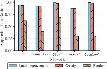
Figure 3: The empirical approximation ratio $\gamma$ for algorithms. The number of vertices and edges ($n$, $m$) for each subgraph are as follows. City*: $(1607,50112)$, Arena*: $(1981,9132)$, Google+*: ($2000$, $5042$).

Representative results for the empirical ratio are shown in Fig. (3). Overall, we observe that the effectiveness of Local-Improvement and Greedy are close to the optimal value, with Local-Improvement outperforming Greedy by a small margin. Specifically, the empirical ratio of Local-Improvement is greater than $0.85$ on all tested instances. As one would expect, the empirical ratio of Random is much lower than its counterparts. Overall, we note that the empirical ratio of Local-Improvement is much higher than its theoretical guarantee of $1/2$. Recall from Section (4) that there are instances where Local-Improvement produces solutions that are of $1/2$ of the optimal value. Our experimental findings indicate such worst-case instances did not occur in these experiments. We also note that empirically Greedy is comparable to Local Improvement. However, no known performance guarantee for Greedy has been established. In contrast, as shown in Section (4), Local Improvement provides a guarantee of $1/2$.

Variations on the number of minority agents. Next, we study the integration ratio $\mu$ obtained by the algorithms under the scenario where the fraction of minority agents $(k)$ increases from $0.01$ to $0.25$. The representative results for Gnp and City networks are shown in Fig. (4). Overall, we observe that as the fraction of minority agents increases, the integration ratio $\mu$ grows monotonically for all algorithms. Similar results are observed for all the chosen networks. Despite the monotonicity observed in the experiments, we remark that the objective value that an algorithm can obtain is general non-monotone as $k$ increases. (A simple example is a star where the objective is maximized for $k=1$ when the type-1 agent is placed at the center. It is easy to verify that as $k$ increases, the optimal objective decreases.)

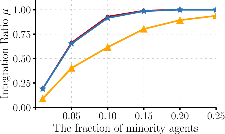
(a) Gnp network

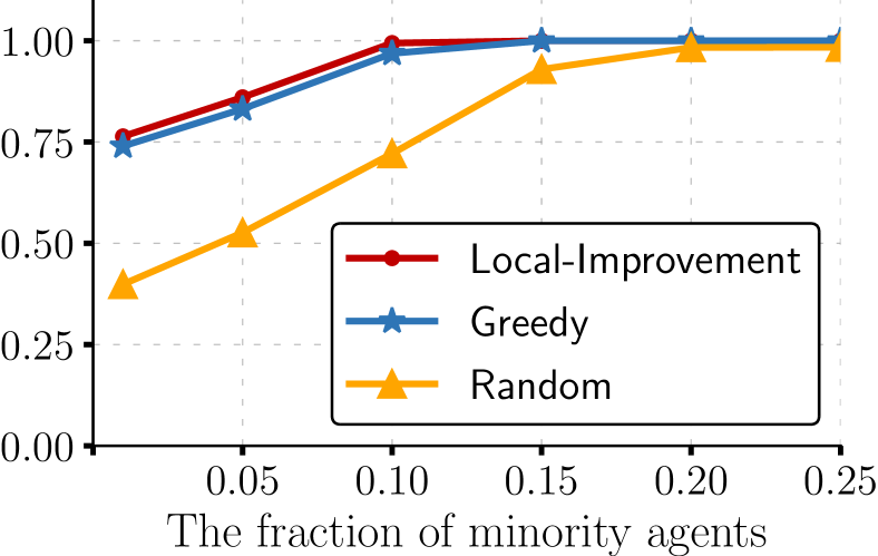
(b) City network

Figure 4: The change of the fraction of integrated agents as the fraction of minority agents increases. The networks are Gnp and City shown in Table (1).

Change of objective as local improvement proceeds. Lastly, we study the increase in the objective value as the number of swaps used in Local-Improvement is increased. Results are shown in Fig. (5) for gnp networks with 1000 nodes and average degrees varying from 10 to 30. Overall, we observe a linear relationship between the objective value and the number of swaps.

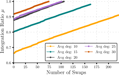
Figure 5: The change in the number of integrated agents as Local-Improvement proceeds. The underlying gnp networks have $1,000$ vertices; the average degree varies from $10$ to $30$.

8 Conclusions

We considered an optimization problem that arises in the context of placing agents on a network to maximize the integration level. Since the general problem is NP-hard, we presented approximation algorithms with provable performance guarantees for several versions of the problem. Our work suggests several directions for further research. First, it is of interest to investigate approximation algorithms with better performance guarantees for the general problem. One possible approach is to consider local improvement algorithms that instead of swapping just one pair of vertices to increase the number of integrated vertices, swap up to $j$ pairs, for some fixed $j\geq 2$ in each iteration. One can also study the problem under network-based extensions of other integration indices proposed in the social science literature [25]. Another direction is the scenario where the total number of agents is less than the number of nodes (so that some nodes remain unoccupied by agents). In addition, one can also study the variant where there are agents of three or more types, and the notion of integration is defined by requiring the neighborhood of an agent to include a certain number of agents of the other types. Overall, this topic offers a variety of interesting new problems for future research.

Appendix

4 Additional Materials for Section 4

Notation	Definition
$\mathcal{P}$	An assignment return by the algorithm
$\mathcal{P}^{*}$	An optimal assignment
$\mathcal{V}{}_{i}(\mathcal{P})$	The set of type-$i$ vertices under $\mathcal{P}$
$\mathcal{V}^{\texttt{U}}_{i}(\mathcal{P})$	The set of uncovered type-$i$ vertices under $\mathcal{P}$
$\mathcal{N}^{\texttt{U}}_{v}(\mathcal{P})$	The set of neighbors of $v\in\mathcal{V}{}$ that are uncovered under $\mathcal{P}$
$\Gamma_{v}(\mathcal{P})$	The set of different-type neighbors of $v$ that are uniquely covered by $v$
Type-$i$ vertex (under $\mathcal{P}$)	A vertex occupied by a type-$i$ agent
An uncovered vertex (under $\mathcal{P}$)	A vertex that is not integrated

Table 2: A notation table

Agarwal et al. [1] establish that IM-IoA is NP-hard. We now further study its solvability. For convenience in presenting the proofs, we define an assignment from the perspective of vertices of the underlying graph, rather than the perspective of the agents. We remark that the two definitions are equivalent.

Assignment.

An assignment $\mathcal{P}:\mathcal{V}{}\rightarrow\mathcal{A}$ is a function that assigns an agent type in $\{1,2\}$ to each vertex (location) in $\mathcal{V}{}$, such that $k$ vertices are assigned type-1 and $n-k$ vertices are assigned type-2. Given an assignment $\mathcal{P}$, we call a vertex $v$ a type-1 (or type-2) vertex if $\mathcal{P}(v)=1$ (or $\mathcal{P}(v)=2$). Let $\mathcal{V}{}_{1}(\mathcal{P})$ and $\mathcal{V}{}_{2}(\mathcal{P})$ denote the set of type-1 and type-2 vertices under $\mathcal{P}$. Let $\mathcal{V}^{\texttt{U}}_{1}(\mathcal{P})$ and $\mathcal{V}^{\texttt{U}}_{2}(\mathcal{P})$ denote the set of uncovered type-1 and type-2 vertices under $\mathcal{P}$. For each vertex $u$, let $\mathcal{N}^{\texttt{U}}_{u}(\mathcal{P})$ denote the set of neighbors of $u$ that are uncovered under $\mathcal{P}$, and let $\Gamma_{u}(\mathcal{P})$ denote the set of different-type neighbors of $u$ that are uniquely covered by $u$, i.e., $\Gamma_{u}(\mathcal{P})$ is the set of vertices $v$ such that $(i)$ $v$ is a neighbor of $u$, $(ii)$ the type of $v$ is different from the type of $u$, and $(iii)$ $v$ has no other neighbors whose types are the same as $u$’s type.

4.1 Analysis of the algorithm

We now investigate the performance of Algorithm (1). Let $\mathcal{P}$ be a saturated assignment returned by Algorithm (1). All the analyses are given under $\mathcal{P}$ unless specified otherwise. Recall that $\mathcal{V}^{\texttt{U}}_{1}(\mathcal{P})\subseteq\mathcal{V}{}$ is the set of type-1 vertices are not integrated under $\mathcal{P}$. That is, for each vertex $x\in\mathcal{V}^{\texttt{U}}_{1}(\mathcal{P})$, all neighbors of $x$ under $\mathcal{P}$ are also of type-1. Similarly, let $\mathcal{V}^{\texttt{U}}_{2}(\mathcal{P})\subseteq\mathcal{V}{}$ be the set of type-2 vertices who are not integrated under $\mathcal{P}$. An example of such sets are given in Figure (6).

Observation 4.1.

The index $\texttt{IoA}(\mathcal{P})=n-|\mathcal{V}^{\texttt{U}}_{1}(\mathcal{P})|-|\mathcal{V}^{\texttt{U}}_{2}(\mathcal{P})|$.

We now consider the following mutually exclusive and collectively exhaustive cases of $\mathcal{V}^{\texttt{U}}_{1}(\mathcal{P})$ and $\mathcal{V}^{\texttt{U}}_{2}(\mathcal{P})$ under the saturated assignment $\mathcal{P}$. We start with a simple warm-up case where all the type-2 vertices under $\mathcal{P}$ are integrated.

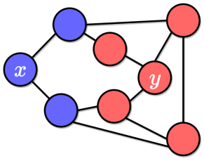
Figure 6: An assignment where type-1 and type-2 vertices are highlighted in blue and red, respectively. In this example, $\mathcal{V}^{\texttt{U}}_{1}(\mathcal{P})=\{x\}$ and $\mathcal{V}^{\texttt{U}}_{2}(\mathcal{P})=\{y\}$. Note that this example is only to demonstrate how the two sets are defined, as later we show that if both $\mathcal{V}^{\texttt{U}}_{1}(\mathcal{P})\neq\emptyset$ and $\mathcal{V}^{\texttt{U}}_{2}(\mathcal{P})\neq\emptyset$, this assignment cannot be a saturated assignment.

Case 1: $\mathcal{V}^{\texttt{U}}_{2}(\mathcal{P})=\emptyset$.

Under this case, all vertices in $\mathcal{V}{}_{2}(\mathcal{P})$ are integrated which gives

$$\texttt{IoA}(\mathcal{P})\geq|\mathcal{V}^{\texttt{U}}_{2}(\mathcal{P})|=n-k\geq\frac{1}{2}\cdot n$$ (18)

The above case trivially implies a $2$-approximation of the algorithm. We now look at the case where $\mathcal{V}^{\texttt{U}}_{2}(\mathcal{P})\neq\emptyset$.

Case 2: $\mathcal{V}^{\texttt{U}}_{2}(\mathcal{P})\neq\emptyset$.

Under this case, there exists at least one vertex in $\mathcal{V}{}_{2}(\mathcal{P})$ that is not integrated. We now study the approximation ratio.

Lemma 4.2.

For a saturated assignment $\mathcal{P}$, if $\mathcal{V}^{\texttt{U}}_{2}(\mathcal{P})\neq\emptyset$, then $\mathcal{V}^{\texttt{U}}_{1}(\mathcal{P})=\emptyset$.

Proof.

Let $y\in\mathcal{V}^{\texttt{U}}_{2}(\mathcal{P})$ be a vertex of type-2 that is not integrated (i.e., all neighbors of $y$ are of type-2). For contradiction, suppose $\mathcal{V}^{\texttt{U}}_{1}(\mathcal{P})\neq\emptyset$.. Now let $x\in\mathcal{V}^{\texttt{U}}_{1}(\mathcal{P})$ be an non-integrated vertex of type-1 whose neighbors are all of type-1. Let $\mathcal{P}^{\prime}$ denote the assignment where we switch the types between $x$ and $y$, that is, $\mathcal{P}^{\prime}(x)=\mathcal{P}(y)=\texttt{2}$, $\mathcal{P}^{\prime}(y)=\mathcal{P}(x)=\texttt{1}$, while the types of all other vertices remain unchanged.

Claim 4.2.1.

$\texttt{IoA}(\mathcal{P}^{\prime})\geq\texttt{IoA}(\mathcal{P})+2$, that is, switching the types of $x$ and $y$ increases the index IoA by at least $2$.

We now establish the above claim. First observe that after the switch, only the integration status of vertices in $\{x,y\}\cup\mathcal{N}(x)\cup\mathcal{N}(y)$ can change, where $\mathcal{N}(x)$ and $\mathcal{N}(y)$ are neighbors of $x$ and $y$. Given that all neighbors of $x$ are of type-1 under $\mathcal{P}$, and $y$ is of type-2, switching $\mathcal{P}(x)$ with $\mathcal{P}(y)$ can only increase the number of integrated neighbors in $\mathcal{N}(x)$. Similarly, switching $\mathcal{P}(y)$ with $\mathcal{P}(x)$ can only increase the number of integrated neighbors in $\mathcal{N}(y)$. Further, note that $x$ (who was not integrated in $\mathcal{P}$) will be integrated after the switch, as $\mathcal{N}(x)$ consists of (only) vertices of type-1. By the same argument, $y$ (who was again not integrated in $\mathcal{P}$) will be integrated after the switch. It follows that after the switch, the index IoA would increase by at least $2$, that is, $\texttt{IoA}(\mathcal{P}^{\prime})\geq\texttt{IoA}(\mathcal{P})+2$. This conclude the claim. One may check Figure (6) for a visualization.

The claim implies the existence of an improvement move from $\mathcal{P}$, which contradicts $\mathcal{P}$ being a saturated assignment. It follows that no such an $x\in\mathcal{V}^{\texttt{U}}_{1}(\mathcal{P})$ exists and thus $\mathcal{V}^{\texttt{U}}_{1}(\mathcal{P})=\emptyset$. ∎

Lemma (4.2) immediately implies that under case 2 (i.e., $\mathcal{V}^{\texttt{U}}_{2}(\mathcal{P})\neq\emptyset$), we must have $\mathcal{V}^{\texttt{U}}_{1}(\mathcal{P})=\emptyset$.

$$\texttt{IoA}(\mathcal{P})\geq|\mathcal{V}_{1}|=k$$ (19)

We now argue for a stronger approximation ratio of $2$. Consider the following two mutually exclusive and collectively exhaustive subcases under Case $2$. Recall that for each vertex $x$, $\Gamma_{x}(\mathcal{P})$ is the set of different-type neighbors of $x$ that are uniquely covered (i.e. “made integrated”) by $x$ under $\mathcal{P}$. Formally, if $x\in\mathcal{V}{}_{1}(\mathcal{P})$, then $\Gamma_{x}(\mathcal{P})=\{y\in\mathcal{V}{}_{2}(\mathcal{P})\cup\mathcal{N}(x)\;:\;y\notin\bigcup_{x^{\prime}\in\mathcal{V}{}_{1}(\mathcal{P})\setminus\{x\}}\mathcal{N}(x^{\prime})\}$

Subcase 2.1: $\mathcal{V}^{\texttt{U}}_{2}(\mathcal{P})\neq\emptyset$, and

$$\Gamma_{x}(\mathcal{P})\neq\emptyset,\;\;\forall x\in\mathcal{V}{}_{1}(\mathcal{P})$$

that is, for each type-1 vertex $x\in\mathcal{V}{}_{1}(\mathcal{P})$, there is at least one type-2 neighbors $y$ of $x$ that is uniquely covered (i.e. “made integrated“) by $x$.

Recall that $\mathcal{P}$ is a saturated assignment returned by the algorithm. By Lemma (4.2), we know that all vertices in $\mathcal{V}{}_{1}(\mathcal{P})$ are integrated under $\mathcal{P}$. Thus, the total number of integrated vertices under $\mathcal{P}$ equals $|\mathcal{V}{}_{1}(\mathcal{P})|=k$ plus the number of vertices in $\mathcal{V}{}_{2}(\mathcal{P})$ that are adjacent to vertices in $\mathcal{V}{}_{1}(\mathcal{P})$ (It immediately follows that $\texttt{IoA}(\mathcal{P})\geq 2\cdot\frac{k}{n}$). Let $\mathcal{P}^{*}$ by an optimal assignment that gives the maximum number of integrated vertices. We now argue that $\texttt{IoA}(\mathcal{P})\geq\frac{1}{2}\cdot\texttt{IoA}(\mathcal{P}^{*})$.

Suppose $\mathcal{P}\neq\mathcal{P}^{*}$, that is, for some $x\in\mathcal{V}{}$, $\mathcal{P}(x)\neq\mathcal{P}^{*}(x)$. Let $\tilde{\mathcal{V}{}}_{2-1}=\{v\in\mathcal{V}{}\;:\;\mathcal{P}(v)=2,\mathcal{P}^{*}(v)=1\}$ be the set of vertices that are type-2 under $\mathcal{P}$, but are type-1 under $\mathcal{P}^{*}$. Analogously, let $\tilde{\mathcal{V}{}}_{1-2}=\{v\in\mathcal{V}{}\;:\;\mathcal{P}(v)=1,\mathcal{P}^{*}(v)=2\}$ be the set of vertices of type-1 under $\mathcal{P}$, but are of type-2 under $\mathcal{P}^{*}$. Observe that $|\tilde{\mathcal{V}{}}_{2-1}|=|\tilde{\mathcal{V}{}}_{1-2}|$. We may view $\mathcal{P}^{*}$ as the result of a transformation from $\mathcal{P}$ under pairwise swaps of types between $\tilde{\mathcal{V}{}}_{2-1}$ and $\tilde{\mathcal{V}{}}_{1-2}$. An example is given in Figure (7). We present a key lemma that bounds the difference in the objective value between $\mathcal{P}$ and $\mathcal{P}^{*}$.

Figure 7: Two assignments $\mathcal{P}$ and $\mathcal{P}^{*}$ where type-1 and type-2 vertices are highlighted in blue and red, respectively. In this case, $\tilde{\mathcal{V}{}}_{2-1}=\{x_{3},x_{4}\}$ and $\tilde{\mathcal{V}{}}_{1-2}=\{x_{1},x_{2}\}$. We may then transform $\mathcal{P}$ into $\mathcal{P}^{*}$ by swapping types between the pair $(x_{1},x_{3})$ and between $(x_{2},x_{4})$. Note that this example is only to demonstrate how $\tilde{\mathcal{V}{}}_{2-1}$ and $\tilde{\mathcal{V}{}}_{1-2}$ are defined, as $\mathcal{P}$ cannot be a saturated assignment returned by the algorithm.

Lemma 4.3 (Subcase 2.1).

Let $\mathcal{P}$ be a saturated assignment that satisfies subcase 2.1, and let $\mathcal{P}^{*}$ be an optimal assignment. We have

$$\texttt{IoA}(\mathcal{P}^{*})-\texttt{IoA}(\mathcal{P}) \leq\sum_{y\in\tilde{\mathcal{V}{}}_{2-1}\setminus\mathcal{V}^{\texttt{U}}_{2}(\mathcal{P})}|(\mathcal{N}(y)\cap\mathcal{V}^{\texttt{U}}_{2}(\mathcal{P})|+\sum_{y\in\tilde{\mathcal{V}{}}_{2-1}\cap\mathcal{V}^{\texttt{U}}_{2}(\mathcal{P})}\left(|(\mathcal{N}(y)\cap\mathcal{V}^{\texttt{U}}_{2}(\mathcal{P})|+1\right)$$ (20)

Proof.

Since $\mathcal{P}$ is saturated, Lemma (4.2) implies that all type-1 vertices under $\mathcal{P}$ are integrated. Thus, $\texttt{IoA}(\mathcal{P}^{*})-\texttt{IoA}(\mathcal{P})$ is at most the number of type-2 vertices that are integrated under $\mathcal{P}^{*}$ but are not integrated under $\mathcal{P}$.

Let $f:\tilde{\mathcal{V}{}}_{1-2}\rightarrow\tilde{\mathcal{V}{}}_{2-1}$ be an arbitrary bijective mapping. We may regard $\mathcal{P}^{*}$ as a result of the transformation from $\mathcal{P}$ via pairwise swaps of types between vertices specified by $f$ (i.e., the type of $x\in\tilde{\mathcal{V}{}}_{1-2}$ is swapped with the type of $f(x)\in\tilde{\mathcal{V}{}}_{2-1}$). Observe that only vertices in $\mathcal{V}^{\texttt{U}}_{2}(\mathcal{P})$ that are adjacent to $\tilde{\mathcal{V}{}}_{2-1}$ (or within $\tilde{\mathcal{V}{}}_{2-1}$) under $\mathcal{P}$ can be newly integrated under $\mathcal{P}^{*}$ after swapping $\tilde{\mathcal{V}{}}_{1-2}$ with $\tilde{\mathcal{V}{}}_{2-1}$ (by the definition of $\mathcal{V}^{\texttt{U}}_{2}(\mathcal{P})$, vertices in $\tilde{\mathcal{V}{}}_{1-2}$ have no neighbors in $\mathcal{V}^{\texttt{U}}_{2}(\mathcal{P})$.). It follows that for each vertex $y\in\tilde{\mathcal{V}{}}_{2-1}$, at most $|(\mathcal{N}(y)\cap\mathcal{V}^{\texttt{U}}_{2}(\mathcal{P})|$ of its neighbors can become newly integrated after transforming from $\mathcal{P}$ to $\mathcal{P}^{*}$. Further, if also $y\in\tilde{\mathcal{V}{}}_{2-1}\cap\mathcal{V}^{\texttt{U}}_{2}(\mathcal{P})$, $y$ itself could also be newly integrated after the swap. We then have

$$\texttt{IoA}(\mathcal{P}^{*})-\texttt{IoA}(\mathcal{P}) \leq|\bigcup_{y\in\tilde{\mathcal{V}{}}_{2-1}}\mathcal{N}(y)\cap\mathcal{V}^{\texttt{U}}_{2}(\mathcal{P})|+|\tilde{\mathcal{V}{}}_{2-1}\cap\mathcal{V}^{\texttt{U}}_{2}(\mathcal{P})|$$ (21)

$$\leq\sum_{y\in\tilde{\mathcal{V}{}}_{2-1}\setminus\mathcal{V}^{\texttt{U}}_{2}(\mathcal{P})}|(\mathcal{N}(y)\cap\mathcal{V}^{\texttt{U}}_{2}(\mathcal{P})|+\sum_{y\in\tilde{\mathcal{V}{}}_{2-1}\cap\mathcal{V}^{\texttt{U}}_{2}(\mathcal{P})}\left(|(\mathcal{N}(y)\cap\mathcal{V}^{\texttt{U}}_{2}(\mathcal{P})|+1\right)$$ (22)

where the last inequality follows from the union bound. This completes the proof. ∎

We note that the bound derived in Lemma (4.3) is not tight for many problem instances. Nevertheless, later we will see that such a bound is enough for our purpose of showing a $\frac{1}{2}$ approximation. Further, we note that there indeed exist a class of problem instances where this bound is exact.

Lemma (4.3) bounds the maximum difference between $\texttt{IoA}(\mathcal{P}^{*})$ and $\texttt{IoA}(\mathcal{P})$, which is

$$\sum_{y\in\tilde{\mathcal{V}{}}_{2-1}\setminus\mathcal{V}^{\texttt{U}}_{2}(\mathcal{P})}|(\mathcal{N}(y)\cap\mathcal{V}^{\texttt{U}}_{2}(\mathcal{P})|+\sum_{y\in\tilde{\mathcal{V}{}}_{2-1}\cap\mathcal{V}^{\texttt{U}}_{2}(\mathcal{P})}\left(|(\mathcal{N}(y)\cap\mathcal{V}^{\texttt{U}}_{2}(\mathcal{P})|+1\right)$$

We now proceed to show that the above difference is at most $\texttt{IoA}(\mathcal{P})$, thereby establishing $\texttt{IoA}(\mathcal{P})\geq\frac{1}{2}\cdot\texttt{IoA}(\mathcal{P}^{*})$. All the discussion below are under $\mathcal{P}$ unless stated otherwise. Recall that for each vertex $x\in\mathcal{V}{}$, $\Gamma_{x}(\mathcal{P})$ is the set of neighbors of $x$ whose types are different from $x$, and are uniquely covered by $x$ under $\mathcal{P}$. By the definition of Subcase $2.1$, $\Gamma_{x}(\mathcal{P})$ is not empty for all $x\in\mathcal{V}{}_{1}(\mathcal{P})$. We first argue that for any $y\in\mathcal{V}^{\texttt{U}}_{2}(\mathcal{P})$ and any $x\in\mathcal{V}{}_{1}(\mathcal{P})$, we have $|\mathcal{N}(y)\cap\mathcal{V}^{\texttt{U}}_{2}(\mathcal{P})|\leq|\Gamma_{x}(\mathcal{P})|$.

Lemma 4.4 (Subcase 2.1).

Given a saturated assignment $\mathcal{P}$, for any $y\in\mathcal{V}^{\texttt{U}}_{2}(\mathcal{P})$ and any $x\in\mathcal{V}{}_{1}(\mathcal{P})$, we have

$$|\mathcal{N}(y)\cap\mathcal{V}^{\texttt{U}}_{2}(\mathcal{P})|\leq|\Gamma_{x}(\mathcal{P})|$$

Proof.

Given that $y$ is not integrated under $\mathcal{P}$, $x$ and $y$ cannot be adjacent. Since $\mathcal{P}$ is a saturated assignment, if the types of $x$ and $y$ are to be swapped, the number of newly integrated vertices would be at most the number of newly non-integrated vertices. We now examine the integration status of vertices in the closed neighborhood of $x$ and $y$ under $\mathcal{P}$ after such a swap:

$$\text{For }y\text{ and its neighbors}\left\{\begin{array}[]{lr}\text{All vertices in }\mathcal{N}(y)\cap\mathcal{V}^{\texttt{U}}_{2}(\mathcal{P})\text{ become}\textit{ newly integrated}\\ \text{All vertices in }\mathcal{N}(y)\cap(\mathcal{A}_{2}\setminus\mathcal{V}^{\texttt{U}}_{2}(\mathcal{P}))\text{ remain integrated}\\ \text{The vertex }y\text{ itself }\text{becomes {\em newly integrated}}\end{array}\right\}$$

$$\text{For }x\text{ and its neighbors}\left\{\begin{array}[]{lr}\text{All vertices in }\mathcal{N}(x)\setminus\Gamma_{x}(\mathcal{P})\text{ remain integrated}\\ \text{Some vertices in }\Gamma_{x}(\mathcal{P})\text{ {may} become newly {non}-integrated}\\ \text{The vertex }x\text{ itself }\text{ {may} become newly {non}-integrated}\end{array}\right\}$$

Overall, the number of vertices that are newly integrated is at least $|\mathcal{N}(y)\cap\mathcal{V}^{\texttt{U}}_{2}(\mathcal{P})|+1$, and the number of vertices that are newly non-integrated is at most $|\Gamma_{x}(\mathcal{P})|+1$. Since $\mathcal{P}$ is saturated, it follows that:

$$|\mathcal{N}(y)\cap\mathcal{V}^{\texttt{U}}_{2}(\mathcal{P})|\leq|\Gamma_{x}(\mathcal{P})|$$ (23)

This concludes the proof. ∎

We now show that for any $y\in\mathcal{V}{}_{2}(\mathcal{P})\setminus\mathcal{V}^{\texttt{U}}_{2}(\mathcal{P})$ and any $x\in\mathcal{V}{}_{1}(\mathcal{P})$, we have $|\mathcal{N}(y)\cap\mathcal{V}^{\texttt{U}}_{2}(\mathcal{P})|\leq|\Gamma_{x}(\mathcal{P})|+1$.

Lemma 4.5 (Subcase 2.1).

Given a saturated assignment $\mathcal{P}$, for any $y\in\mathcal{V}{}_{2}(\mathcal{P})\setminus\mathcal{V}^{\texttt{U}}_{2}(\mathcal{P})$ and any $x\in\mathcal{V}{}_{1}(\mathcal{P})$, we have

$$|\mathcal{N}(y)\cap\mathcal{V}^{\texttt{U}}_{2}(\mathcal{P})|\leq|\Gamma_{x}(\mathcal{P})|+1$$

Proof.

We partition $\mathcal{V}{}_{2}(\mathcal{P})\setminus\mathcal{V}^{\texttt{U}}_{2}(\mathcal{P})$ into two subsets $\mathcal{B}$ and $\mathcal{C}$, as follows. Subset $\mathcal{B}$ is the set of integrated type-2 vertices whose neighbors are all integrated under $\mathcal{P}$, i.e.,

$$\mathcal{B}=\{y\in\mathcal{V}{}_{2}(\mathcal{P})\setminus\mathcal{V}^{\texttt{U}}_{2}(\mathcal{P})\;:\;\mathcal{N}(y)\cap\mathcal{V}^{\texttt{U}}_{2}(\mathcal{P})=\emptyset\}$$

Subset $\mathcal{C}$, the complement of $\mathcal{B}$, is the set of integrated type-2 vertices with at least one non-integrated neighbor under $\mathcal{P}$, i.e., $\mathcal{C}=\{y\in\mathcal{V}{}_{2}(\mathcal{P})\setminus\mathcal{V}^{\texttt{U}}_{2}(\mathcal{P})\;:\;\mathcal{N}(y)\cap\mathcal{V}^{\texttt{U}}_{2}(\mathcal{P})\neq\emptyset\}$. The Lemma clearly holds if $y\in\mathcal{B}$ since then $|\mathcal{N}(y)\cap\mathcal{V}^{\texttt{U}}_{2}(\mathcal{P})|=0$. We now present a key claim for the case when $y\in\mathcal{C}$:

Claim 4.5.1.

For all vertices $y\in\mathcal{C}$, no type-1 neighbors of $y$ is uniquely covered by $y$ under $\mathcal{P}$ (i.e., $\Gamma_{y}(\mathcal{P})=\emptyset$).

For contradiction, suppose there exists a type-1 neighbors $x\in\mathcal{N}(y)\cap\mathcal{V}{}_{1}(\mathcal{P})$ of $y$ such that $x$ is not adjacent to any other type-2 vertices under $\mathcal{P}$. Then by the definition of subcase 2.1 (i.e., each type-1 vertex uniquely covers at least one type-2 vertex), $x$ is the only type-1 neighbor of $y$. One then can easily verify that exchanging the types between $x$ and $y$ strictly increase the objective of $\mathcal{P}$, contradicting the fact that $\mathcal{P}$ is saturated. This conclude the proof of Claim (4.5.1).

We continue to assume that $y\in\mathcal{C}$ and consider an objective non-increasing move from $\mathcal{P}$ where we swap the types between $x$ and $y$. If $y$ is a neighbor of $x$ under $\mathcal{P}$, then by Claim (4.5.1), one can verify that the the maximum loss is $|\Gamma_{x}(\mathcal{P})|$ and the minimum gain is $|\mathcal{N}(y)\cap\mathcal{V}^{\texttt{U}}_{2}(\mathcal{P})|$. Thus

$$|\mathcal{N}(y)\cap\mathcal{V}^{\texttt{U}}_{2}(\mathcal{P})|\leq|\Gamma_{x}(\mathcal{P})|$$ (24)

On the other hand, if $y$ is not a neighbor of $x$ under $\mathcal{P}$, one can verify that the maximum loss is $|\Gamma_{x}(\mathcal{P})|+1$ and the minimum gain is $|\mathcal{N}(y)\cap\mathcal{V}^{\texttt{U}}_{2}(\mathcal{P})|$. Thus

$$|\mathcal{N}(y)\cap\mathcal{V}^{\texttt{U}}_{2}(\mathcal{P})|\leq|\Gamma_{x}(\mathcal{P})|+1$$ (25)

This concludes the proof. ∎

We are now ready to establish $\texttt{IoA}(\mathcal{P})\geq\frac{1}{2}\cdot\texttt{IoA}(\mathcal{P}^{*})$ under Subcase 2.1.

Lemma 4.6 (Subcase 2.1).

Suppose $\mathcal{V}^{\texttt{U}}_{2}(\mathcal{P})\neq\emptyset$ and $\Gamma_{x}(\mathcal{P})\neq\emptyset,\forall x\in\mathcal{V}{}_{1}(\mathcal{P})$, we have

$$\texttt{IoA}(\mathcal{P})\geq\frac{1}{2}\cdot\texttt{IoA}(\mathcal{P}^{*})$$

where $\mathcal{P}^{*}$ is an optimal assignment that gives the maximum objective.

Proof.

Note that $\tilde{\mathcal{V}{}}_{2-1}$ is a subset of $\mathcal{V}{}_{2}(\mathcal{P})$. Further, Observe that $\Gamma_{x}(\mathcal{P})$ are disjoint for different vertices $x\in\mathcal{V}{}_{1}(\mathcal{P})$. Now, by Lemma (4.3) to and (4.5), We have

$$\texttt{IoA}(\mathcal{P}^{*})-\texttt{IoA}(\mathcal{P})$$

$$\leq\sum_{y\in\tilde{\mathcal{V}{}}_{2-1}\setminus\mathcal{V}^{\texttt{U}}_{2}(\mathcal{P})}|(\mathcal{N}(y)\cap\mathcal{V}^{\texttt{U}}_{2}(\mathcal{P})|+\sum_{y\in\tilde{\mathcal{V}{}}_{2-1}\cap\mathcal{V}^{\texttt{U}}_{2}(\mathcal{P})}\left(|(\mathcal{N}(y)\cap\mathcal{V}^{\texttt{U}}_{2}(\mathcal{P})|+1\right)\;\;\;\;\;\;\;\;(\text{Lemma}~{}(\ref{lem:subcase1-bound}))$$

$$\leq\sum_{y\in\tilde{\mathcal{V}{}}_{2-1}\setminus\mathcal{V}^{\texttt{U}}_{2}(\mathcal{P})}(|\Gamma_{f^{-1}(y)}(\mathcal{P})|+1)+\sum_{y\in\tilde{\mathcal{V}{}}_{2-1}\cap\mathcal{V}^{\texttt{U}}_{2}(\mathcal{P})}(|\Gamma_{f^{-1}(y)}(\mathcal{P})|+1)\;\;\;\;\;\;\;\;(\text{Lemma}~{}(\ref{lemma:subcase2.1-1})\;\&~{}(\ref{lemma:subcase2.1-2}))$$

$$=\left(\sum_{y\in\tilde{\mathcal{V}{}}_{2-1}}|\Gamma_{f^{-1}(y)}(\mathcal{P})|\right)+|\tilde{\mathcal{V}{}}_{2-1}|$$

$$\leq|\mathcal{V}{}_{2}(\mathcal{P})\setminus\mathcal{V}^{\texttt{U}}_{2}(\mathcal{P})|+|\mathcal{V}{}_{1}(\mathcal{P})|$$ (26)

$$\leq\texttt{IoA}(\mathcal{P})$$

where Inequality (26) follows from $|\tilde{\mathcal{V}{}}_{2-1}|=|\tilde{\mathcal{V}{}}_{1-2}|\leq|\mathcal{V}{}_{1}(\mathcal{P})|$ and $\left(\sum_{y\in\tilde{\mathcal{V}{}}_{2-1}}|\Gamma_{f^{-1}(y)}(\mathcal{P})|\right)\leq|\mathcal{V}{}_{2}(\mathcal{P})\setminus\mathcal{V}^{\texttt{U}}_{2}(\mathcal{P})|$. This concludes the proof. ∎

We now have shown that if $\mathcal{V}^{\texttt{U}}_{2}(\mathcal{P})\neq\emptyset$ and $\Gamma_{x}(\mathcal{P})\neq\emptyset,\forall x\in\mathcal{V}{}_{1}(\mathcal{P})$, the algorithm gives a 2 approximation. We proceed to the last subcase.

Subcase 2.2: $\mathcal{V}^{\texttt{U}}_{2}(\mathcal{P})\neq\emptyset$, and

$$\Gamma_{x}(\mathcal{P})=\emptyset,\;\;\;\exists x\in\mathcal{V}{}_{1}(\mathcal{P})$$

that is, there exists at least one type-1 vertex $x\in\mathcal{V}{}_{1}(\mathcal{P})$ such that for each type-2 neighbor $y$ of $x$, $y$ is adjacent to at least one type-1 vertex other than $x$.

Lemma 4.7 (Subcase 2.2).

Under subcase 2.2, for each non-integrated type-2 vertex $y\in\mathcal{V}^{\texttt{U}}_{2}(\mathcal{P})$, all type-2 neighbors of $y$ are integrated (i.e., $\mathcal{N}(y)\cap\mathcal{V}^{\texttt{U}}_{2}(\mathcal{P})=\emptyset$) under $\mathcal{P}$.

Proof.

Given such a $x\in\mathcal{V}{}_{1}(\mathcal{P})$ defined in Subcase 2.2, for contradiction, suppose there is a non-integrated type-2 vertex $y\in\mathcal{V}^{\texttt{U}}_{2}(\mathcal{P})$ s.t. at least one type-2 neighbor, denoted by $y^{\prime}\in\mathcal{N}(y)$, of $y$ is not integrated under $\mathcal{P}$ (note that all neighbors of $y$ are of type-2 since $y$ is not integrated). Now consider a new assignment $\mathcal{P}^{\prime}$ where we switch the types between $x$ and $y$.

Claim 4.7.1.

We have $\texttt{IoA}(\mathcal{P}^{\prime})\geq\texttt{IoA}(\mathcal{P})+1$, that is, after the switch, the index IoA would increase by at least $1$.

We now establish the claim. Similar to Lemma (4.2), only the integration status of vertices in $\{x,y\}\cup\mathcal{N}(x)\cup\mathcal{N}(y)$ can change. We first consider the integration states of vertices in $\mathcal{N}(x)$. Let $\texttt{IoA}(\mathcal{N}(x),\mathcal{P})$ denote the number of integrated vertices in the neighborhood of $x$ under $\mathcal{P}$, and let $\Delta\texttt{IoA}(\mathcal{N}(x),\mathcal{P})=\texttt{IoA}(\mathcal{N}(x),\mathcal{P}^{\prime})-\texttt{IoA}(\mathcal{N}(x),\mathcal{P})$ denote the change in the integrated vertices in the neighborhood of $x$ after the switch. Let $\mathcal{N}_{\texttt{1}}(x,\mathcal{P})$ and $\mathcal{N}_{\texttt{2}}(x,\mathcal{P})$ denote the set of type-1 and type-2 neighbors of $x$ under $\mathcal{P}$, respectively.

Under Subcase $2.2$, each vertex $\mathcal{N}_{\texttt{2}}(x,\mathcal{P})$ is adjacent to at least one type-1 vertex in additional to $x$, thus, all vertices in $N_{\texttt{2}}(x,\mathcal{P})$ remain integrated after we swap types between $y$ and $x$. Further, it is easy to see that the swap cannot decrease the number of integrated vertices in $\mathcal{N}_{\texttt{1}}(x,\mathcal{P})$. It follows that

$$\Delta\texttt{IoA}(\mathcal{N}(x),\mathcal{P})\geq 0$$

Now consider the integration states of vertices in $\mathcal{N}(y)$. First observe that $\mathcal{N}_{\texttt{1}}(y,\mathcal{P})=\emptyset$ since $y\in\mathcal{V}^{\texttt{U}}_{2}(\mathcal{P})$ is not integrated. Also, swapping the types between $y$ and $x$ will not decrease the number of integrated vertices in $\mathcal{N}_{\texttt{2}}(y,\mathcal{P})$. In fact, since there exists a vertex $y^{\prime}\in\mathcal{N}_{\texttt{2}}(y,\mathcal{P})$ who is not integrated under $\mathcal{P}$, the swap makes $y^{\prime}$ integrated (as $x$ and $y^{\prime}$ are of different types). It follows that

$$\Delta\texttt{IoA}(\mathcal{N}(y),\mathcal{P})\vcentcolon=\texttt{IoA}(\mathcal{N}(y),\mathcal{P}^{\prime})-\texttt{IoA}(\mathcal{N}(y),\mathcal{P})\geq 1$$

Lastly, we consider the integration states of $x$ and $y$. In particular, $x$ is integrated under $\mathcal{P}$, and after the swap, it might become non-integrated. On the other hand, $y$ is not integrated under $\mathcal{P}$, it must become newly integrated after the swap. Nevertheless, the net increase of the number of integrated vertices in $\{x,y\}$ is at least $0$ when we change from $\mathcal{P}$ to $\mathcal{P}^{\prime}$. Overall, it follows that

$$\texttt{IoA}(\mathcal{P}^{\prime})-\texttt{IoA}(\mathcal{P})=\Delta\texttt{IoA}(\mathcal{N}(x),\mathcal{P})+\Delta\texttt{IoA}(\mathcal{N}(y),\mathcal{P})+\Delta\texttt{IoA}(\{x,y\},\mathcal{P})\geq 1$$ (27)

This concludes the claim. Note that the claim implies the existence of an improvement move from $\mathcal{P}$, which contradicts $\mathcal{P}$ being a saturated assignment returned by Algorithm (1). Thus, no such a non-integrated type-2 vertex $y^{\prime}$ of $y$ can exist, that is, for each $y\in\mathcal{V}^{\texttt{U}}_{2}(\mathcal{P})$, all (type-2) neighbors of $y$ are integrated. This concludes the proof. ∎

Lemma (4.7) implies that under Subcase 2.2, the vertices in $\mathcal{V}^{\texttt{U}}_{2}(\mathcal{P})$ form an independent set of $\mathcal{G}$, as stated in the corollary below.

Corollary 4.7.1 (Subcase 2.2).

Under Subcase 2.2, vertices in $\mathcal{V}^{\texttt{U}}_{2}(\mathcal{P})$ form an independent set of $\mathcal{G}$.

Observe that $\texttt{IoA}(\mathcal{P})=(n-|\mathcal{V}^{\texttt{U}}_{2}(\mathcal{P})|)$. Using Lemma (4.7), we now argue the size of $\mathcal{V}^{\texttt{U}}_{2}(\mathcal{P})$ cannot be too large.

Lemma 4.8 (Subcase 2.2).

Under Subcase 2.2, we have

$$|\mathcal{V}^{\texttt{U}}_{2}(\mathcal{P})|\leq\frac{n}{2}$$

Proof.

Let

$$\mathcal{Y}\vcentcolon=\{y\in\mathcal{V}{}_{2}(\mathcal{P})\setminus\mathcal{V}^{\texttt{U}}_{2}(\mathcal{P})\;:\;\mathcal{N}(y)\cap\mathcal{V}^{\texttt{U}}_{2}(\mathcal{P})\neq\emptyset\}$$

be the set of type-2 integrated vertices whose has at least one non-integrated type-2 neighbor. Recall that $\Gamma_{y}(\mathcal{P})$ is the set of type-1 neighbors of $y$ who are uniquely covered by $y$ under $\mathcal{P}$. We first note that $\Gamma_{y}(\mathcal{P})$ (if not empty) are mutually disjoint for different $y\in\mathcal{Y}$. It follows that

$$\texttt{IoA}(\mathcal{P})\geq|\mathcal{Y}|+\sum_{y\in\mathcal{Y}}|\Gamma_{y}(\mathcal{P})|$$ (28)

Now revisit the definition of subcase 2.2. In particular there exists a type-1 vertex $x\in\mathcal{V}{}_{1}(\mathcal{P})$ such that each type-2 neighbor of $x$ is also covered by (i.e., adjacent to) at least one other type-1 vertex. Suppose we switch the types between such a vertex $x$ and a vertex $y\in\mathcal{Y}$, and let $\mathcal{P}^{\prime}$ denote the resulting new assignment. Observe the following in $\mathcal{P}^{\prime}$

Claim 4.8.1.

All vertices in $\mathcal{N}(x)$ remains integrated in $\mathcal{P}^{\prime}$.

This holds since these neighbors are either of $(i)$ type-1 which are now adjacent to $x$ of type-2 in $\mathcal{P}^{\prime}$, or of $(ii)$ type-2 which are adjacent to at least one other type-1 vertex.

Claim 4.8.2.

All vertices in $\mathcal{N}(y)\cap\mathcal{V}^{\texttt{U}}_{2}(\mathcal{P})$ become newly integrated in $\mathcal{P}^{\prime}$, and all vertices in $\Gamma_{y}(\mathcal{P})$ may become newly non-integrated in $\mathcal{P}^{\prime}$. The integration status of all other vertices in $\mathcal{N}(y)$ remain unchanged from $\mathcal{P}$ to $\mathcal{P}^{\prime}$.

One can easily verify the above claim based on the fact that $y$ is of type-1 under $\mathcal{P}^{\prime}$. Lastly, note that in $y$ remains integrated in $\mathcal{P}^{\prime}$ since $y$ is of type-1 in $\mathcal{P}^{\prime}$ and has at least one type-2 neighbor. On the other hand, $x$ (who was integrated in $\mathcal{P}$) might not be integrated in $\mathcal{P}^{\prime}$. It follows that the maximum loss of objective after the swap is $|\Gamma_{y}(\mathcal{P})|+1$, where as the minimum gain is $|\mathcal{N}(y)\cap\mathcal{V}^{\texttt{U}}_{2}(\mathcal{P})|$. Since $\mathcal{P}$ is a saturated assignment returned by the algorithm, we must have $\texttt{IoA}(\mathcal{P})\geq\texttt{IoA}(\mathcal{P}^{\prime})$. It follows that

$$|\mathcal{N}(y)\cap\mathcal{V}^{\texttt{U}}_{2}(\mathcal{P})|\leq|\Gamma_{y}(\mathcal{P})|+1,\;\forall y\in\mathcal{Y}$$ (29)

Lastly, by Corollary (4.7.1), vertices in $\mathcal{V}^{\texttt{U}}_{2}(\mathcal{P})$ form an independent set of $G$. Thus,

$$|\mathcal{V}^{\texttt{U}}_{2}(\mathcal{P})|=|\bigcup_{y\in\mathcal{Y}}\mathcal{N}(y)\cap\mathcal{V}^{\texttt{U}}_{2}(\mathcal{P})|$$ (30)

Overall, we have that

$$|\mathcal{V}^{\texttt{U}}_{2}(\mathcal{P})| =|\bigcup_{y\in\mathcal{Y}}\mathcal{N}(y)\cap\mathcal{V}^{\texttt{U}}_{2}(\mathcal{P})|\;\;\;\;\;\;\;\;\;\;\;\;\;\;\;\;\;\;\;\;\;(\text{Corollary~{}(\ref{coro:indpendent-set})}$$ (31)

$$\leq\sum_{y\in\mathcal{Y}}|\mathcal{N}(y)\cap\mathcal{V}^{\texttt{U}}_{2}(\mathcal{P})|\;\;\;\;\;\;\;\;\;\;\;\;\;\;\;\;\;\;\;\;\;\;(\text{Union bound})$$ (32)

$$\leq\sum_{y\in\mathcal{Y}}(|\Gamma_{y}(\mathcal{P})|+1)\;\;\;\;\;\;\;\;\;\;\;\;\;\;\;\;\;\;\;\;\;\;\;\;\;\;\;(\text{Eq.~{}(\ref{eq:1/2-subcase2}}))$$ (33)

$$\leq|\mathcal{V}{}_{1}(\mathcal{P})|+|\mathcal{Y}|\;\;\;\;\;\;\;\;\;\;\;\;\;\;\;\;\;\;\;\;\;\;\;\;\;\;\;\;\;\;\;\;\;(\text{$\Gamma_{y}(\mathcal{P})$ are mutually disjoint})$$ (34)

$$\leq|\mathcal{V}{}_{1}(\mathcal{P})|+|\mathcal{V}{}_{2}(\mathcal{P})\setminus\mathcal{V}^{\texttt{U}}_{2}(\mathcal{P})|\;\;\;\;\;\;\;\;\;(\text{By }\mathcal{Y}\subseteq\mathcal{V}{}_{2}(\mathcal{P})\setminus\mathcal{V}^{\texttt{U}}_{2}(\mathcal{P}))$$ (35)

$$=n-|\mathcal{V}^{\texttt{U}}_{2}(\mathcal{P})|$$ (36)

It immediately follows that

$$|\mathcal{V}^{\texttt{U}}_{2}(\mathcal{P})|\leq\frac{n}{2}$$ (37)

This concludes the proof. ∎

Lastly, Since $\texttt{IoA}(\mathcal{P})=n-|\mathcal{V}^{\texttt{U}}_{2}(\mathcal{P})|$, by Lemma (4.8), we have $\texttt{IoA}(\mathcal{P})=n-|\mathcal{V}^{\texttt{U}}_{2}(\mathcal{P})|\geq\frac{1}{2}\cdot n\geq\frac{1}{2}\cdot\texttt{IoA}(\mathcal{P}^{*})$, thereby establishing a $1/2$ approximation for Subcase 2.2. Overall, we have shown that a saturated assignment $\mathcal{P}$ returned by Algorithm (1) gives a $2$-approximation for IM-IoA. The Theorem immediately follows.

Theorem 4.9.

Algorithm (1) gives a $\frac{1}{2}$-approximation for IM-IoA.

4.1.1 Analysis is tight

We now present a class of problem instances where the approximation ratio of the solution produced by Algorithm (1) can be arbitrarily close to $1/2$. Therefore, the ratio $1/2$ in the statement of Theorem (4.9) cannot be improved, so our analysis is tight.

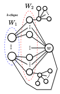
Figure 8: A pictorial example of a problem instance where Algorithm (1) gives an assignment whose approximation ratio is $\frac{1}{2}$.

Proposition 4.10.

For every $\epsilon>0$, there exists a problem instance of IM-IoA for which there is a saturated assignment $\mathcal{P}$ such that $\texttt{IoA}(\mathcal{P})\leq(\frac{1}{2}+\epsilon)\cdot\textsc{OPT}$.

Proof.

Recall that $k$ is the number of type-1 vertices. We first present the construction of the graph $\mathcal{G}{}=(\mathcal{V}{},\mathcal{E}{})$. Let $\mathcal{W}{}_{1}$ be a set of $k$ vertices that form a clique. For each $v\in\mathcal{W}{}_{1}$, we introduce a set $\mathcal{U}_{v}$ of $k$ vertices outside the clique that are adjacent $v$. Let $\mathcal{W}{}_{2}=\bigcup_{v\in\mathcal{W}{}_{1}}\mathcal{U}_{v}$ denote the union of these sets. All vertices in $\mathcal{W}{}_{2}$ are also adjacent to a new vertex $w$, and we further make this vertex $w$ adjacent to exactly one vertex in $\mathcal{W}{}_{1}$. Lastly, we added a total of $k$ stars, each of which consists of $k-1$ vertices (i.e., each star has a center vertex and $k-2$ leaf vertices). We then connect the center of each star to one vertex in a unique $\mathcal{U}_{v}$. This completes the construction. An example is given in Figure (8).

Now consider an assignment $\mathcal{P}$ where all vertices in $\mathcal{W}{}_{1}$ are of type-1 (recall that $k=|\mathcal{W}{}_{1}|$), and the rest of vertices are of type-2. One can verify that such an assignment is saturated (and thus could be returned by Algorithm (1)). On the other hand, an assignment $\mathcal{P}^{*}$ that gives a strictly higher objective is where we assign $(i)$ type-1 to one vertex in $\mathcal{W}{}_{1}$, $(i)$ assign $w$ to type-1, and $(iii)$ the centers of $k-2$ stars (with any two stars being left out) are assigned with type-1. The rest of vertices are of type-2.

One can verify that $\texttt{IoA}(\mathcal{P})=k^{2}+k+1$, and $\texttt{IoA}(\mathcal{P}^{*})=2k^{2}-2k+4$. The ratio $\texttt{IoA}(\mathcal{P})/\texttt{IoA}(\mathcal{P}^{*})=1/2$ as $k$ goes to infinity. Since $\texttt{IoA}(\mathcal{P}^{*})\leq\text{OPT}$ where OPT is the optimal objective of a problem instance, the claim follows. ∎

5 Additional Material for Section 5

We study the problem instances when the number of type-1 agents is a constant fraction of the total number of agents, that is, $k=\alpha\cdot n$ for some constant $0\leq\alpha\leq 1/2$. We refer to this problem as $\alpha n$-IM-IoA. For example, $\alpha=1/2$ implies the bisection constraint.

5.1 Intractability remains

We first show that $\alpha n$-IM-IoA problem remains intractable.

Theorem 5.1.

The problem $\alpha n$-IM-IoA is NP-hard.

Proof.

We present a reduction from the general IM-IoA problem to $\alpha n$-IM-IoA where $\alpha=\frac{1}{2}$. Let $\Pi_{1}=\langle\mathcal{G}{},\mathcal{A}{},n\rangle$ be an instance of IM-IoA, $\mathcal{A}{}=\{\mathcal{A}{}_{1},\mathcal{A}{}_{2}\}$, where $k=|\mathcal{A}{}_{1}|$ is the number of type-1 agents that needs to be assigned, and $n=|\mathcal{V}{}(\mathcal{G}{})|$ is the total number of agents. The decision question asks whether there exists an assignment of agent-types for $\Pi_{1}$ such that all the $n$ vertices are integrated. This question is known to be NP-hard [1].

An instance, $\Pi_{2}=\langle\mathcal{G}{}^{\prime},\mathcal{A}{}^{\prime},2n\rangle$, $\mathcal{A}{}^{\prime}=\{\mathcal{A}{}_{1}^{\prime},\mathcal{A}{}_{2}^{\prime}\}$, of the bisection version of IM-IoA consists of the following components. To from the graph $\mathcal{G}{}^{\prime}$, the first component $\mathcal{G}{}_{1}$ a copy of $\mathcal{G}{}$. Let $\mathcal{G}{}_{2}$ be a graph formed by first creating a simple path $I$ with $k-1$ vertices, then for each vertex $v$ on the path, we introduce a new vertex (not on the path) that is uniquely adjacent to $v$. Overall, $\mathcal{G}{}_{2}$ has $2k-2$ vertices. An example of $\mathcal{G}{}_{2}$ is shown in Figure (9). Let $\mathcal{G}{}_{3}$ be a star graph with $n-2k+2$ vertices (i.e., one center with $n-2k+1$ leaf vertices). Lastly, the final graph $\mathcal{G}{}^{\prime}$ consists of the three aforementioned connected components: $\mathcal{G}{}_{1}$, $\mathcal{G}{}_{2}$, and $\mathcal{G}{}_{3}$. One can verify that $\mathcal{G}{}^{\prime}$ has $2n$ vertices (and thus the number of agents is $2n$). We set the number of type-1 agents $|\mathcal{A}{}_{1}^{\prime}|=n$, corresponding to the bisection constraint $|\mathcal{A}{}_{1}^{\prime}|=1/2\cdot|\mathcal{A}{}^{\prime}|$.

We now argue that $\Pi_{1}$ admits an assignment where all $n$ vertices are integrated if and only if $\Pi_{2}$ has an assignment where all $2n$ vertices are integrated.

• Suppose $\Pi_{1}$ has an assignment $\mathcal{P}$ on $\mathcal{G}{}$ such that all vertices are integrated. We now present an assignment $\mathcal{P}^{\prime}$ for $\mathcal{G}{}^{\prime}$ such that all vertices are integrated in $\Pi_{2}$. Specifically, we discuss how types are assigned on $\mathcal{G}{}_{1}$, $\mathcal{G}{}_{2}$, and $\mathcal{G}{}_{3}$. The assignment of agent-type on $\mathcal{G}{}_{1}$ is the same as that of on $\mathcal{G}{}$ under $\mathcal{P}$. Next, for $\mathcal{G}{}_{2}$, we set all the $k-1$ vertices on the path $I$ to type-1 (i.e., taken by type-1 agents), and the rest of $k-1$ vertices are of type-2. Lastly, for $\mathcal{G}{}_{3}$, all the $n-2k+1$ leaf vertices are of type-1, and the center vertex is of type-2. The completes the construction of $\mathcal{P}^{\prime}$. One can verify that the total number of type-1 vertices is $k+(k-1)+(n-2k+1)=n$, and further, all the $2n$ vertices are integrated under $\mathcal{P}^{\prime}$.

• Suppose $\Pi_{2}$ has an assignment $\mathcal{P}^{\prime}$ on $\mathcal{G}{}^{\prime}$ such that all vertices are integrated. We show that there exists an assignment $\mathcal{P}$ on $\mathcal{G}{}$ such that all vertices are integrated in $\Pi_{1}$. Consider the assignment $\mathcal{P}^{\prime}$ restricted to $\mathcal{G}{}_{2}$ and $\mathcal{G}{}_{3}$. We first observe that any assignment that makes all vertices in $\mathcal{G}{}_{2}$ integrated must has exactly $k-1$ type-1 vertices in $\mathcal{G}{}_{2}$. As for $\mathcal{G}{}_{3}$, there are two possible assignments that makes all vertices integrated: either $(i)$ having one type-2 vertex at the center and the leaf vertices are of type-1 or $(ii)$ vise versa. Note that under the first assignment, the total number of type-1 vertices placed on $\mathcal{G}{}_{2}$ and $\mathcal{G}{}_{3}$ is $(k-1)+(n-2k+1)=n-k$. Since the total number of type-1 vertices is $n$, there are exactly $k$ type-1 vertices in $\mathcal{G}{}_{1}$. Thus, the assignment $\mathcal{P}$ is obtained by restricting $\mathcal{P}^{\prime}$ to $\mathcal{G}{}_{1}$. On the other hand, under the second type of assignment in $\mathcal{G}{}_{3}$, the total number of type-1 vertices placed in $\mathcal{G}{}_{2}$ and $\mathcal{G}{}_{3}$ is $(k-1)+1=k$. That is, there are $n-k$ type-1 vertices in $\mathcal{G}{}_{1}$ under $\mathcal{P}^{\prime}$. Then $\mathcal{P}$ is obtained by flipping the types of vertices (i.e., type-1 changes to type-2, vise versa) assigned in $\mathcal{G}{}_{1}$ under $\mathcal{P}^{\prime}$.

This concludes the proof. ∎

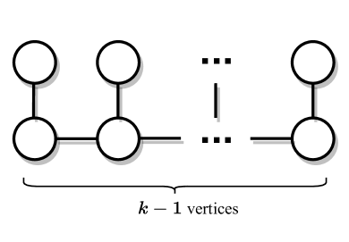
Figure 9: An example of graph $\mathcal{G}{}_{2}$

5.2 A semidefinite programming approach

Our approximation results are given in terms of the expected approximation ratio $\gamma$. One can obtain a w.h.p. bound by $(i)$ running the algorithm $K$ rounds, and $(ii)$ output the best solution. In particular, one can verify that for each round, the probability of producing an approximation factor $(1-\epsilon)\cdot\gamma$ is at least $1-(1-\gamma)/(1-(1-\epsilon)\cdot\gamma)$ for arbitrarily small constant $\epsilon>0$. One can then choose a large enough $K$ to obtain a high probability bound, while $K$ remains a polynomial of $n$.

We now present an approximation algorithm based on a semidefinite programming (SDP) relaxation. Given a graph $\mathcal{G}{}=(\mathcal{V}{},\mathcal{E}{})$, each vertex $i\in\mathcal{V}{}$ has a binary variable $x_{i}\in\{-1,1\}$ such that $x_{i}=-1$ if $i$ is of type-1, and $x_{i}=1$ if $i$ is of type-2. To start with, a quadratic program (QP) of $\alpha n$-IM-IoA and its SDP relaxation can be formulated as follows:

$$\text{QP}:\;\;\;\;\;\text{maximize}\quad \sum_{i\in\mathcal{V}{}}\;\max_{j\in\mathcal{N}(i)}\;\{\frac{1-x_{i}x_{j}}{2}\}$$

s.t. $$\sum_{i<j}x_{i}x_{j}=\frac{(1-2\alpha)^{2}\cdot n^{2}-n}{2}$$

$$x_{i}\in\{-1,1\},\;\;\;\;\;\forall i\in V$$

$$\text{SDP}:\;\;\;\;\;\text{maximize}\quad \sum_{i\in\mathcal{V}{}}\;\max_{j\in\mathcal{N}(i)}\;\{\frac{1-\vec{y}_{i}\cdot\vec{y}_{j}}{2}\}$$

s.t. $$\sum_{i<j}\vec{y}_{i}\cdot\vec{y}_{j}\leq\frac{(1-2\alpha)^{2}\cdot n^{2}-n}{2}$$

$$\vec{y}_{i}\cdot\vec{y}_{i}=1,\;\;\;\;\;\forall i\in V$$

Observation 5.2.

QP is a valid program for the $\alpha n$-IM-IoA problem. Further, if $\textsc{OPT}_{QP}$ and $\textsc{OPT}_{SDP}$ are the optimal solutions to QP and SDP, respectively, we have $\textsc{OPT}_{SDP}\geq\textsc{OPT}_{QP}$.

Note that a naive constraint for an $(\alpha n,(1-\alpha)n)$-paritition is $\sum_{i}x_{i}=(1-2\alpha)\cdot n$. With a simple derivation, one can verify that the constraint $\sum_{i<j}\vec{y}_{i}\cdot\vec{y}_{j}\leq\frac{(1-2\alpha)^{2}\cdot n^{2}-n}{2}$ is equivalent to the constraint $\sum_{i}x_{i}=(1-2\alpha)\cdot n$, as follows:

$$\left(\sum_{i}x_{i}\right)^{2}=\sum_{i}(x_{i})^{2}+2\sum_{i<j}x_{i}x_{j}=n+2\sum_{i<j}x_{i}x_{j}=(1-2\alpha)^{2}\cdot n^{2}$$ (38)

To see that the SDP formulation is indeed a relaxation of the QP, given any feasible solution of the QP, we can construct a feasible solution of the SDP as follows. For each $x_{i}$, we set the first entry in the corresponding $\vec{y}_{i}$ to equal the value of $x_{i}$, and the remaining entries in $\vec{y}_{i}$ to $0$. One can verify that the two solutions have the same objective. It follows that for each solution of the QP, there is a corresponding solution of the SDP with the same objective, thus, $\textsc{OPT}_{SDP}\geq\textsc{OPT}_{QP}$.

First step: Rounding the SDP

We first solve the proposed SDP and obtain the set of vectors $\{\vec{y}_{1},...,\vec{y}_{n}\}$. Let $\textsc{OPT}_{SDP}$ be the optimal objective of the SDP. We want a partition $\{\mathcal{V}{}_{1},\mathcal{V}{}_{2}\}$ of the vertex set such that vertices in $\mathcal{V}{}_{i}$ are of type-$i$, $i=\texttt{1},\texttt{2}$. To do so, we apply Goemans and Williamson’s hyperplane rounding method [15]. In particular, we draw a a random hyperplane thought the origin with a normal vector $r$, and then $\mathcal{V}{}_{1}=\{i:\vec{y}_{i}\cdot r\geq 0\}$ and $\mathcal{V}{}_{2}=\{i:\vec{y}_{i}\cdot r<0\}$. This rounding method has the following desirable property:

Lemma 5.3 (Goemans and Williamson [15]).

The probability that two vertices $i$ and $j$ being in different subsets is $1/\pi\cdot\arccos{}(\vec{y}_{i}\cdot\vec{y}_{j})$.

Consider an assignment $\mathcal{P}$ generated by the above rounding method (i.e., vertices in $\mathcal{V}{}_{i}$ are assigned to type-$i$). Let $f(\mathcal{V}{}_{1}):2^{\mathcal{V}{}}\rightarrow\mathbb{N}$ be the number of integrated vertices under such an assignment. Based on Lemma (5.3), we argue that $f(\mathcal{V}{}_{1})\geq\alpha_{GW}\cdot\textsc{OPT}_{SDP}$ in expectation, where $\alpha_{GW}\geq 0.878567$.

Lemma 5.4.

$\mathbb{E}[f(\mathcal{V}{}_{1})]\geq\alpha_{GW}\cdot\textsc{OPT}_{SDP}$ where $\alpha_{GW}\geq 0.878567$.

Proof.

By Lemma (5.3), for any two vertices $i$ and $j$, let $H_{ij}$ be the event where $i$ and $j$ are in the same subset. we have

$$\Pr[H_{ij}]=1-\frac{\arccos{}(\vec{y}_{i}\cdot\vec{y}_{j})}{\pi}$$ (39)

Let $\mathcal{P}$ be the assignment where we assign type-1 (type-2) to vertices in $\mathcal{V}{}_{1}$ ($\mathcal{V}{}_{2}$). since a vertex $i$ is not integrated if and only if $i$ and all its neighbors are in the same set, we have

$$\Pr[\text{vertex }i\text{ is integrated}] =1-\Pr[\text{vertex }i\text{ is not integrated}]$$

$$=1-\Pr[\bigcap_{j\in\mathcal{N}(i)}H_{ij}]$$

Further,

$$\Pr[\bigcap_{j\in\mathcal{N}(i)}H_{ij}] \leq\min_{j\in\mathcal{N}(i)}\{\;\Pr[H_{ij}]\;\}$$

$$=\min_{j\in\mathcal{N}(i)}\{1-\frac{\arccos{}(\vec{y}_{i}\cdot\vec{y}_{j})}{\pi}\}\;\;\;\;\;\;\;\;(\text{By Eq.}~{}(\ref{eq:Hij}))$$

$$=1-\max_{j\in\mathcal{N}(i)}\{\;\frac{\arccos{}(\vec{y}_{i}\cdot\vec{y}_{j})}{\pi}\;\}$$

and thus

$$\Pr[i\text{ is integrated}]\geq\max_{j\in\mathcal{N}(i)}\{\;\frac{\arccos{}(\vec{y}_{i}\cdot\vec{y}_{j})}{\pi}\;\}$$ (40)

As show in [15], $\arccos{}(z)/\pi\geq\alpha_{GW}\cdot(1-z)/2$ for real $z\in[-1,1]$. It follows that

$$\max_{j\in\mathcal{N}(i)}\{\;\frac{\arccos{}(\vec{y}_{i}\cdot\vec{y}_{j})}{\pi}\;\}\geq\alpha_{GW}\cdot\max_{j\in\mathcal{N}(i)}\{\frac{1-\vec{y}_{i}\cdot\vec{y}_{j}}{2}\}$$ (41)

since $\vec{y}_{i}\cdot\vec{y}_{j}\in[-1,1]$. Recall that $f(\mathcal{V}{}_{1})$ is the number of integrated vertices under the assignment where type-1 (type-2) are assigned to $\mathcal{V}{}_{1}$ ($\mathcal{V}{}_{2}$). We have

$$\mathbb{E}[f(\mathcal{V}{}_{1})] \geq\sum_{i\in\mathcal{V}{}}\max_{j\in\mathcal{N}(i)}\{\;\frac{\arccos{}(\vec{y}_{i}\cdot\vec{y}_{j})}{\pi}\;\}$$ (42)

$$\geq\alpha_{GW}\cdot\sum_{i\in\mathcal{V}{}}\max_{j\in\mathcal{N}(i)}\{\frac{1-\vec{y}_{i}\cdot\vec{y}_{j}}{2}\}$$ (43)

$$\geq\alpha_{GW}\cdot\textsc{OPT}_{SDP}$$ (44)

This concludes the proof. ∎

Second step: Fix the size

In the previous step, we have shown that given a partition $\{\mathcal{V}{}_{1},\mathcal{V}{}_{2}\}$ resulted from hyperplane rounding, if all vertices in $\mathcal{V}{}_{1}$ are of type-1, and all vertices in $\mathcal{V}{}_{2}$ are of type-2, then the expected number of integrated vertices is at least $\alpha_{GW}$ of the optimal. Nevertheless, there is one problem: the partition is not necessarily an $(\alpha n,1-\alpha)n$-partition. In this section, we present an algorithm to move vertices from one subset to another such that $(i)$ the resulting new partition is an $(\alpha n,(1-\alpha)n)$-partition, and $(ii)$ the objective does not decrease “too much” after the moving process.

1

Input : Subsets $\mathcal{V}{}_{1}$ and $\mathcal{V}{}_{2}$

Output : Subsets $\mathcal{V}{}_{1}^{(T)}$ and $\mathcal{V}{}_{2}^{(T)}$, where $T=|\mathcal{V}{}_{1}|-\alpha n$

2

3$\mathcal{V}{}_{1}^{(0)}\leftarrow\mathcal{V}{}_{1}$, $\mathcal{V}{}_{2}^{(0)}\leftarrow\mathcal{V}{}_{2}$

4for $t$ from $1$ to $T$ do

5       $i\leftarrow\operatorname*{arg\,max}_{j\in\mathcal{V}{}_{1}^{(t-1)}}\{f(\mathcal{V}{}_{1}^{(t-1)}\setminus\{j\})-f(\mathcal{V}{}_{1}^{(t-1)})\}$

6      $\mathcal{V}{}_{1}^{(t)}\leftarrow\mathcal{V}{}_{1}^{(t-1)}\setminus\{i\}$

7      $\mathcal{V}{}_{2}^{(t)}\leftarrow\mathcal{V}{}_{2}^{(t-1)}\cup\{i\}$

return $\{\mathcal{V}{}_{1}^{(T)},\mathcal{V}{}_{2}^{(T)}\}$

Algorithm 2 Fix-Size

Algorithm for the second step.

Without losing generality, suppose $|\mathcal{V}{}_{1}|\geq\alpha n$. Overall, our algorithm consists of $T=|\mathcal{V}{}_{1}|-\alpha n$ iterations, and in each each iteration, we move a vertex $i\in\mathcal{V}{}_{1}$ to $\mathcal{V}{}_{2}$. Specifically, let $\mathcal{V}{}_{1}^{(t)}$ be the subset at the $t$th iteration, with $\mathcal{V}{}_{1}^{(0)}=\mathcal{V}{}_{1}$. To obtain $\mathcal{V}{}_{1}^{(t+1)}$, we choose $i\in\mathcal{V}{}_{1}^{(t)}$ to be a vertex that maximizes $f(\mathcal{V}{}_{1}^{(t)}\setminus\{i\})-f(\mathcal{V}{}_{1}^{(t)})$, and the move $i$ to the other subset. A pseudocode is given in Algorithm (2).

Let $\mathcal{V}{}_{1}^{(T)}$, $T=|\mathcal{V}{}_{1}|-\alpha n$, be the subset returned by Algorithm (2).

Lemma 5.5.

We have

$$\frac{f(\mathcal{V}{}_{1}^{(T)})}{|\mathcal{V}{}_{1}^{(T)}|}\geq\frac{f(\mathcal{V}{}_{1})}{|\mathcal{V}{}_{1}|}$$

Proof.

For each vertex $j\in\mathcal{V}{}_{1}^{(t)}$, $0\leq t\leq T-1$, let $\eta_{j}^{(t)}$ be the number of its neighbors in $\mathcal{V}{}_{2}^{(t)}$ that are not adjacent to any other vertices in $\mathcal{V}{}_{1}^{(t)}$. Further, let $\nu^{(t)}$ be the number of vertices in $\mathcal{V}{}_{2}^{(t)}$ that have more than one neighbor in $\mathcal{V}{}_{1}^{(t)}$, and let $\delta^{(t)}$ be the number of vertices in $\mathcal{V}{}_{1}^{(t)}$ that has at least one neighbor in $\mathcal{V}{}_{2}^{(t)}$. We then have that $f(\mathcal{V}{}_{1}^{(t)})=\delta^{(t)}+\nu^{(t)}+\sum_{j\in\mathcal{V}{}_{1}^{(t)}}\eta_{j}^{(t)}$, thus

$$\frac{f(\mathcal{V}{}_{1}^{(t)})}{|\mathcal{V}{}_{1}^{(t)}|}=\frac{\delta^{(t)}+\nu^{(t)}+\sum_{j\in\mathcal{V}{}_{1}^{(t)}}\eta_{j}^{(t)}}{|\mathcal{V}{}_{1}^{(t)}|}$$

We now argue that

$$\frac{f(\mathcal{V}{}_{1}^{(t)})}{|\mathcal{V}{}_{1}^{(t)}|}\leq\frac{f(\mathcal{V}{}_{1}^{(t+1)})}{|\mathcal{V}{}_{1}^{(t+1)}|}$$ (45)

Note that if there exists at least one vertex in $\mathcal{V}{}_{1}^{(t)}$ that has no neighbors in $\mathcal{V}{}_{2}^{(t)}$ (i.e., $\delta^{(t)}<|\mathcal{V}{}_{1}^{(t)}|$), then such a vertex will be chosen. One can easily verify that the resulting new objective $f(\mathcal{V}{}_{1}^{(t+1)})$ is greater than $f(\mathcal{V}{}_{1}^{(t)})$ and the above inequality (45) clearly holds.

Now suppose that all vertices in $\mathcal{V}{}_{1}^{(t)}$ have neighbors on the other side. Note that after moving any vertex $j$ from $\mathcal{V}{}_{1}^{(t)}$ to $\mathcal{V}{}_{2}^{(t)}$, the decrease of the objective is at most $\eta_{j}+1$, where the additional plus one comes from the possibility of $j$ itself becoming non-integrated. By the greedy nature of the algorithm, we have that $f(\mathcal{V}{}_{1}^{(t)})-f(\mathcal{V}{}_{1}^{(t+1)})\leq\eta_{min}+1$, where $\eta_{min}=\min_{j}\{\eta_{j}\}$. It follows that

$$\frac{f(\mathcal{V}{}_{1}^{(t+1)})}{|\mathcal{V}{}_{1}^{(t+1)}|} \geq\frac{f(\mathcal{V}{}_{1}^{(t)})-\eta_{min}-1}{|\mathcal{V}{}_{1}^{(t)}|-1}$$

$$=\frac{\delta^{(t)}-1}{|\mathcal{V}{}_{1}^{(t)}|-1}+\frac{\nu^{(t)}}{|\mathcal{V}{}_{1}^{(t)}|-1}+\frac{\left(\sum_{j\in\mathcal{V}{}_{1}^{(t)}}\eta_{j}^{(t)}\right)-\eta_{min}}{|\mathcal{V}{}_{1}^{(t)}|-1}$$

$$\geq\frac{\delta^{(t)}}{|\mathcal{V}{}_{1}^{(t)}|}+\frac{\nu^{(t)}}{|\mathcal{V}{}_{1}^{(t)}|}+\frac{\left(\sum_{j\in\mathcal{V}{}_{1}^{(t)}}\eta_{j}^{(t)}\right)}{|\mathcal{V}{}_{1}^{(t)}|}$$ (46)

$$=\frac{f(\mathcal{V}{}_{1}^{(t)})}{|\mathcal{V}{}_{1}^{(t)}|}$$

Lastly, by recursion, we have that

$$\frac{f(\mathcal{V}{}_{1}^{(T)})}{|\mathcal{V}{}_{1}^{(T)}|}\geq\frac{f(\mathcal{V}{}_{1}^{(0)})}{|\mathcal{V}{}_{1}^{(0)}|}=\frac{f(\mathcal{V}{}_{1})}{|\mathcal{V}{}_{1}|}$$ (47)

This concludes the proof. ∎

The final algorithm.

We have defined the two steps (i.e., $(i)$ round the SDP and $(ii)$ fix the sizes of the two subsets) that we need to take to obtain a feasible solution of the problem. Let $\epsilon\geq 0$ be a small constant, and let $L=\lceil\log_{a}({\frac{1}{\epsilon}})\rceil$ where $a=[(1+\beta)-(1-\epsilon)2\alpha_{GW}]/(1+\beta-2\alpha_{GW})$, $\beta=1/(4(\alpha-\alpha^{2}))$. Note that $L$ is a constant w.r.t. $n$. The final algorithm consists of $L$ iterations, where each iteration performs the two steps defined above. This gives us $L$ feasible solutions. The algorithm then outputs a solution with the highest objective.

Analysis of the final algorithm

Theorem 5.6.

The final algorithm gives a factor

$$\frac{\alpha\left((1-\epsilon)\cdot 2\alpha_{GW}-\frac{\gamma-\gamma^{2}}{\alpha-\alpha^{2}}\right)}{\gamma}\cdot(1-\epsilon)$$

approximation w.h.p. where $\alpha_{GW}\geq 0.878567$, $\epsilon\geq 0$ is an arbitrarily small positive constant, $\alpha=k/n$ is the fraction of minority agents in the group, and $\gamma=\sqrt{\alpha(1-\alpha)(1-\epsilon)\cdot 2\alpha_{GW}}$.

Proof.

The analysis of the final algorithm follows a same route as the one in [13]. For any iteration $1\leq\ell\leq L$ of the algorithm, let $\mathcal{V}{}_{1}$ and $\hat{\mathcal{V}{}}_{1}$ be the subsets returned after the first step and the second step, respectively. In Lemma (5.5), we have shown that

$$\frac{f(\hat{\mathcal{V}{}_{1}})}{|\hat{\mathcal{V}{}_{1}}|}\geq\frac{f(\mathcal{V}{}_{1})}{|\mathcal{V}{}_{1}|}\cdot$$ (48)

Let $X=f(\mathcal{V}{}_{1})$ be a random variable denoting the objective of the solution after the rounding, before performing the second step. Let $Y=|\mathcal{V}{}_{1}|\cdot|\mathcal{V}{}_{2}|$ be another random variable, representing the product of the sizes of the two partitions. Lemma (5.3) have shown that $\mathbb{E}[X]\geq\alpha_{GW}\cdot\textsc{OPT}_{SDP}$. For the expected value of $Y$, we have

$$\mathbb{E}[Y] =\sum_{i<j}\Pr[i\text{ and }j\text{ are in different subset}]$$

$$\geq\alpha_{GW}\cdot\sum_{i<j}\frac{1-\vec{y}_{i}\cdot\vec{y}_{j}}{2}$$ (49)

where the second inequality follows from Lemma (5.3). By the SDP constraint $\sum_{i<j}\vec{y}_{i}\cdot\vec{y}_{j}\leq[(1-2\alpha)^{2}\cdot n^{2}-n]/2$, we can further show that

$$\sum_{i<j}1-\vec{y}_{i}\cdot\vec{y}_{j} =\frac{n(n-1)}{2}-\sum_{i<j}\vec{y}_{i}\cdot\vec{y}_{j}$$

$$\geq\frac{n(n-1)}{2}-\frac{(1-2\alpha)^{2}\cdot n^{2}-n}{2}$$ (50)

$$=\frac{\left((2-2\alpha)\cdot 2\alpha\right)\cdot n^{2}}{2}$$

It follows that

$$\mathbb{E}[Y]\geq\alpha_{GW}\cdot\frac{\left((2-2\alpha)\cdot 2\alpha\right)\cdot n^{2}}{4}=\alpha_{GW}\cdot(\alpha-\alpha^{2})\cdot n^{2}$$ (51)

Let $N=(\alpha-\alpha^{2})\cdot n^{2}$. Let random variable $Z=X/\textsc{OPT}_{SDP}+Y/N$, then $\mathbb{E}[Z]\geq 2\cdot\alpha_{GW}$. Further, since $Y\leq n^{2}/4$, one can verify that $Y/N\leq 1/(4(\alpha-\alpha^{2}))$. Overall, we have $Z\leq 1+\beta$ where $\beta=1/(4(\alpha-\alpha^{2}))$.

With simple Markov inequality, we have

$$\Pr[Z\leq(1-\epsilon)\cdot 2\alpha_{GW}]\leq\frac{(1+\beta)-2\alpha_{GW}}{(1+\beta)-(1-\epsilon)\cdot 2\alpha_{GW}}$$ (52)

Note that there is a random variable $Z$ for each of the iteration. Define $Z^{\prime}$ to be the largest $Z$ over all the $L$ iterations where $Z^{\prime}=X^{\prime}/\textsc{OPT}_{SDP}+Y^{\prime}/N$. It follows that

$$\Pr[Z^{\prime}\leq(1-\epsilon)\cdot 2\alpha_{GW}]\leq\left(\frac{(1+\beta)-2\alpha_{GW}}{(2+\beta)-(1-\epsilon)\cdot 2\alpha_{GW}}\right)^{L}\leq\epsilon$$ (53)

For our choice of $L=\lceil\log_{a}(1/\epsilon)\rceil$ where $a=[(1+\beta)-(1-\epsilon)\cdot 2\alpha_{GW}]/(1+\beta-2\alpha_{GW})$. We consider the case where

$$Z^{\prime}\geq(1-\epsilon)\cdot 2\alpha_{GW}$$

which happens with probability at least $1-\epsilon$. Let $\rho=X^{\prime}/\textsc{OPT}_{SDP}$ be the ratio of $X^{\prime}$ to the optimal of SDP. Then by the definition $Z^{\prime}=X^{\prime}/\textsc{OPT}_{SDP}+Y^{\prime}/N$, one can verify that

$$Y^{\prime}\geq\left((1-\epsilon)\cdot 2\alpha_{GW}-\rho\right)N$$ (54)

Let $\mu=|\mathcal{V}{}_{1}^{\prime}|\;/\;n$ where $\mathcal{V}{}_{1}^{\prime}$ is the subset for type-1 vertices obtained after the first step (i.e., rounding) in the iteration for $Z^{\prime}$. Then $Y^{\prime}=\mu(1-\mu)n^{2}$. Using equation (54) and $N=(\alpha-\alpha^{2})n^{2}$, we can verify that

$$\rho\geq(1-\epsilon)\cdot 2\alpha_{GW}-\frac{\mu-\mu^{2}}{\alpha-\alpha^{2}}$$ (55)

Now let $\hat{\mathcal{V}{}}_{1}^{\prime}$ be the subset of type-1 vertices after fixing the size of $\mathcal{V}{}_{1}^{\prime}$ (i.e., after the second step). Based on Lemma (5.5) and equation (55), we have

$$f(\hat{\mathcal{V}{}}_{1}^{\prime}) \geq\frac{f(\mathcal{V}{}_{1}^{\prime})}{|\mathcal{V}{}_{1}^{\prime}|}\cdot|\hat{\mathcal{V}{}}_{1}^{\prime}|$$ (56)

$$=\frac{f(\mathcal{V}{}_{1}^{\prime})\cdot\alpha}{\mu}$$ (57)

$$=\frac{\alpha\cdot\rho}{\mu}\cdot\textsc{OPT}_{SDP}$$ (58)

$$\geq\frac{\alpha\left((1-\epsilon)\cdot 2\alpha_{GW}-\frac{\mu-\mu^{2}}{\alpha-\alpha^{2}}\right)}{\mu}\cdot\textsc{OPT}_{SDP}$$ (59)

One can verify that for $\mu>0$, $\frac{\alpha\left((1-\epsilon)\cdot 2\alpha_{GW}-\frac{\mu-\mu^{2}}{\alpha-\alpha^{2}}\right)}{\mu}$ is minimum at $\mu=\sqrt{\alpha(1-\alpha)(1-\epsilon)\cdot 2\alpha_{GW}}$.

Let $\gamma=\sqrt{\alpha(1-\alpha)(1-\epsilon)\cdot 2\alpha_{GW}}$, we then have

$$f(\hat{\mathcal{V}{}}_{1}^{\prime})\geq\frac{\alpha\left((1-\epsilon)\cdot 2\alpha_{GW}-\frac{\gamma-\gamma^{2}}{\alpha-\alpha^{2}}\right)}{\gamma}\cdot\textsc{OPT}_{SDP}$$ (60)

Lastly, since $\Pr[Z^{\prime}>(1-\epsilon)\cdot 2\alpha_{GW}]\geq 1-\epsilon$,

$$\mathbb{E}[f(\hat{\mathcal{V}{}}_{1}^{\prime})]\geq\frac{\alpha\left((1-\epsilon)\cdot 2\alpha_{GW}-\frac{\gamma-\gamma^{2}}{\alpha-\alpha^{2}}\right)}{\gamma}\cdot(1-\epsilon)\cdot\textsc{OPT}_{SDP}$$ (61)

∎

For small enough $\epsilon$, say $\epsilon=10^{-3}$, the approximation ratio is greater than $1/2$ for $\alpha$ in range $[0.4,0.5]$. For example, $\alpha=0.45$ gives a ratio of $0.5781$, and $\alpha=0.5$ gives a ratio of $0.6492$.

6 Additional Material for Section 6

In this section, we first show that IM-IoA can be solved in polynomial time on treewidth bounded graphs. Based on this result, we further present a polynomial time approximation scheme (PTAS) for the problem on planar graphs.

6.1 A dynamic programming algorithm for treewidth bounded graphs

The concept treewidth of a graph is first introduced in the seminal work by Robertson and Seymour [32]. Many intractable problems have since enjoyed polynomial time algorithms when underlying graphs have bounded treewidth. In this section, we present a dynamic programming algorithm that solves IM-IoA in polynomial time (w.r.t. $n$) for the class of graphs that are treewidth bounded.

Dynamic programming setup.

Given an instance of IM-IoA with graph $\mathcal{G}=(\mathcal{V}{},\mathcal{E}{})$ and the number $k$ of minorities, let $\mathcal{T}=(\mathcal{I},\mathcal{F})$ be a tree decomposition of $\mathcal{G}{}$ with a bounded treewidth $\sigma$. For each $\mathcal{X}_{i}\in\mathcal{I}$, consider the set of bags in the subtree rooted at $\mathcal{X}_{i}$ in $\mathcal{T}$, and let $\mathcal{Y}_{i}$ be the set of all vertices in these bags. Let $\mathcal{G}{}[\mathcal{Y}_{i}]$ denote the graph $\mathcal{G}{}$ induced on $\mathcal{Y}_{i}$. For each bag $\mathcal{X}_{i}$, we define an array $H_{i}$ to keep track of the optimal objectives in $\mathcal{G}{}[\mathcal{Y}_{i}]$.

A naive definition that fails.

One immediate way is to define $H_{i}(S,\gamma)$ to be the optimal objective in $\mathcal{G}{}[\mathcal{Y}_{i}]$ such that $(i)$ $S\subseteq\mathcal{X}_{i}$ are of type-1, $\mathcal{X}_{i}\setminus S$ are of type-2; $(ii)$ there are a total of $\gamma$ type-1 vertices and $|\mathcal{Y}_{i}|-r$ type-2 vertices in $\mathcal{G}{}[\mathcal{Y}_{i}]$. As a result, for each $\mathcal{X}_{i}$, its corresponding $H_{i}$ has $O(2^{\sigma}\cdot n)$ entries, which is polynomial w.r.t. $n$ since $\sigma$ is bounded. Despite the simplicity of this definition, however, it is unclear how to correctly update these arrays. For example, suppose $\mathcal{X}_{i}$ is of the type introduce, let $\mathcal{X}_{j}$ be the child of $\mathcal{X}_{i}$. Let $v\notin S$ be the vertices that is introduced to $\mathcal{X}_{i}$. One might try to update $H_{i}(S,\gamma)$ by doing $H_{i}(S,\gamma)=H_{j}(S,\gamma)+w(v,\mathcal{X}_{i})$, where $w(v,\mathcal{X}_{i})$ is the number of newly integrated vertices in $\mathcal{X}_{i}$ after $v$ being introduced to the set. This formulation looks correct at the first glance since $v$ is not adjacent to any vertices in $\mathcal{Y}_{i}$ other than those in $\mathcal{X}_{i}$. Thus, it seems that the impact this extra vertex $v$ can cause is only restricted within $\mathcal{X}_{i}$. However, we remark this far from true, and that the above computation is not optimal. In particular, consider the example given in Fig (10).

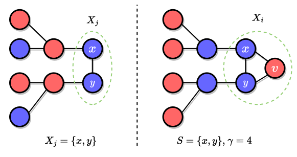
Figure 10: An example where the naive dp approach fails. Given an example graph $\mathcal{G}{}$, the subgraph on the left is $\mathcal{G}{}$ induced on $\mathcal{Y}_{j}$, where $\mathcal{X}_{j}=\{x,y\}$. The subgraph on the right is $\mathcal{G}{}$ induced on $\mathcal{Y}_{i}$, where $\mathcal{X}_{j}=\{x,y,v\}$. The set $S=\{x,y\}$, and $\gamma=4$. Optimal assignments that yields $H_{j}(S,\gamma)$ and $H_{i}(S,\gamma)$ are given where blue vertices are of type-1, and red vertices are of type-2. In particular, $H_{j}(S,\gamma)=6$ and $H_{i}(S,\gamma)=9$. Note that the naive dp approach would set $H_{i}(S,\gamma)$ to be $6+1=7$ which is not optimal.

An alternative definition.

We introduce another dimension to the above definition of $H_{i}$. In particular, let $H_{i}(S,S^{\prime},\gamma)$ be the optimal objective in $\mathcal{G}{}[\mathcal{Y}_{i}]$ such that

• Vertices in the subset $S\subseteq\mathcal{X}_{i}$ are of type-1, and vertices in $\mathcal{X}_{i}\setminus S$ are of type-2.

• Vertices in $S^{\prime}\subseteq\mathcal{X}_{i}$ are to be treated integrated.

• There is a total of $\gamma$ type-1 vertices and $|\mathcal{Y}_{i}|-\gamma$ type-2 vertices in $\mathcal{G}{}[\mathcal{Y}_{i}]$.

The resulting $H_{i}$ has $O(4^{\sigma}\cdot n)$ entries. The algorithm then proceeds in a bottom-up fashion from the leaves to the root in $\mathcal{T}$. We now discuss how the array $H_{i}$ is updated for each bag $\mathcal{X}_{i}$.

Update Scheme

• Leaf: For all $\gamma=0,...,\min\{|\mathcal{Y}_{i}|,k\}$ (recall that $k$ is the total number of type-1 agents) and for all $S\subseteq\mathcal{X}_{i}$ s.t. $|S|=\gamma$, let $Z_{i}(S)$ be the set of integrated vertices in $\mathcal{G}{}[\mathcal{X}_{i}]$ under the assignment $(S,\mathcal{X}_{i}\setminus S)$. For all $S^{\prime}\subseteq X_{i}$, we have

  $$H_{i}(S,S^{\prime},\gamma)=|S^{\prime}\cup Z_{i}(S)|$$ (62)

• Introduce: Let $\mathcal{X}_{j}$ be the child of $\mathcal{X}_{i}$, and let $v$ be the vertex introduced to $\mathcal{X}_{i}$ (i.e., $v\in\mathcal{X}_{i}$ and $v\notin\mathcal{X}_{j}$). For all $\gamma=0,...,\min\{|\mathcal{Y}_{i}|,k\}$, and for all $S\subseteq\mathcal{X}_{i}$ s.t. $|S|\leq\gamma$, let $Z_{i}(S)$ be the set of integrated vertices in $\mathcal{G}{}[\mathcal{X}_{i}]$ under the assignment $(S,\mathcal{X}_{i}\setminus S)$. For all $S^{\prime}\subseteq\mathcal{X}_{i}$:

  • If $v\in S$,

    $$H_{i}(S,S^{\prime},\gamma)=H_{j}(S\setminus\{v\},S^{\prime}\cup Z_{i}(S)\setminus\{v\},\gamma-1)+\mathbbm{1}(v)$$ (63)

  • If $v\notin S$,

    $$H_{i}(S,S^{\prime},\gamma)=H_{j}(S,S^{\prime}\cup Z_{i}(S)\setminus\{v\},\gamma)+\mathbbm{1}(v)$$ (64)

  where $\mathbbm{1}(v)$ is an indicated variable that equals to $1$ if and only if $v$ is integrated in $\mathcal{G}{}[\mathcal{X}_{i}]$ under the assignment $(S,\mathcal{X}_{i}\setminus S)$.

• Forget: Let $\mathcal{X}_{j}$ be the child of $\mathcal{X}_{i}$, and let $v$ be the vertex forgot by $\mathcal{X}_{i}$ (i.e., $v\notin\mathcal{X}_{i}$ and $v\in\mathcal{X}_{j}$). For all $\gamma=0,...,\min\{|\mathcal{Y}_{i}|,k\}$, and for all $S\subseteq\mathcal{X}_{i}$ s.t. $|S|\leq\gamma$, let $Z_{i}(S)$ be the set of integrated vertices in $\mathcal{G}{}[\mathcal{X}_{i}]$ under the assignment $(S,\mathcal{X}_{i}\setminus S)$. For all $S^{\prime}\subseteq\mathcal{X}_{i}$:

  $$H_{i}(S,S^{\prime},\gamma)=\max\{H_{j}(S,Z_{i}(S)\cup S^{\prime},\gamma),H_{j}(S\cup\{v\},Z_{i}(S)\cup S^{\prime},\gamma)\}$$ (65)

• Join: Let $\mathcal{X}_{j1}$ and $\mathcal{X}_{j2}$ be the two children of $\mathcal{X}_{i}$. Note that $\mathcal{X}_{j1}=\mathcal{X}_{j2}=\mathcal{X}_{i}$. For all $\gamma=0,...,\min\{|\mathcal{Y}_{i}|,k\}$, and for all $S\subseteq\mathcal{X}_{i}$ s.t. $|S|\leq\gamma$, let $Z_{i}(S)$ be the set of truly integrated vertices in $\mathcal{G}{}[\mathcal{X}_{i}]$ under the assignment $(S,\mathcal{X}_{i}\setminus S)$.

  For all $S^{\prime}\subseteq\mathcal{X}_{i}$, let $Q_{i}(S,S^{\prime})=\mathcal{X}_{i}\setminus\left(S^{\prime}\cup Z_{i}(S)\right)$ be the set of vertices that are not truly integrated in $\mathcal{G}{}[\mathcal{X}_{i}]$ under the assignment $(S,\mathcal{X}_{i}\setminus S)$, and also should not be treated as integrated (i.e., vertices in $Q_{i}(S,S^{\prime})$ are not in $S^{\prime}$). We consider all subsets $Q_{j1}(S,S^{\prime})\subseteq Q_{i}(S,S^{\prime})$ and $Q_{j2}(S,S^{\prime})\subseteq Q_{i}(S,S^{\prime})$, let $\bar{Q}_{j1}(S,S^{\prime})=Q_{i}(S,S^{\prime})\setminus Q_{j1}(S,S^{\prime})$ and $\bar{Q}_{j2}(S,S^{\prime})=Q_{i}(S,S^{\prime})\setminus Q_{j2}(S,S^{\prime})$.

  Consider the solutions $H_{j1}(S,S^{\prime}\cup Z_{i}(S)\cup\bar{Q}_{j1}(S,S^{\prime}),\gamma_{1})$ and $H_{j2}(S,S^{\prime}\cup Z_{i}(S)\cup\bar{Q}_{j2}(S,S^{\prime}),\gamma_{2})$. Let $\mathcal{P}[Q_{j1}(S,S^{\prime}),\gamma_{1}]$ and $\mathcal{P}[Q_{j2}(S,S^{\prime}),\gamma_{2}]$ be two corresponding assignments, restricted to $\mathcal{Y}_{j1}$ and $\mathcal{Y}_{j2}$, that yield the objective $H_{j1}(S,S^{\prime}\cup Z_{i}(S)\cup\bar{Q}_{j1}(S,S^{\prime}),\gamma_{1})$ and $H_{j2}(S,S^{\prime}\cup Z_{i}(S)\cup\bar{Q}_{j2}(S,S^{\prime}),\gamma_{2})$, respectively. Such assignments can be easily obtained during the bottom-up process. Lastly, let $W(\mathcal{P}[Q_{j1}(S,S^{\prime}),\gamma_{1}])$ and $W(\mathcal{P}[Q_{j2}(S,S^{\prime}),\gamma_{2}])$ be the set of truly integrated vertices in $\mathcal{Y}_{j1}\setminus\left(S^{\prime}\cup Z_{i}(S)\right)$ and $\mathcal{Y}_{j2}\setminus\left(S^{\prime}\cup Z_{i}(S)\right)$ under the assignments $\mathcal{P}[Q_{j1}(S,S^{\prime}),\gamma_{1}]$ and $\mathcal{P}[Q_{j2}(S,S^{\prime}),\gamma_{2}]$, respectively.

  $H_{i}(S,S^{\prime},\gamma)$ is computed as follows

  $$H_{i}(S,S^{\prime},\gamma)=\max_{D}\{|W(\mathcal{P}[Q_{j1}(S,S^{\prime}),\gamma_{1}])\cup W(\mathcal{P}[Q_{j2}(S,S^{\prime}),\gamma_{2}])|\}+|S^{\prime}\cup Z_{i}(S)|$$ (66)

  where

  $$D=\{\gamma_{1},\gamma_{2},Q_{j1}(S,S^{\prime}),Q_{j2}(S,S^{\prime}):\gamma_{1}+\gamma_{2}-|S|=\gamma,\gamma_{1}\geq|S|,\gamma_{2}\geq|S|,Q_{j1}(S,S^{\prime})\subseteq Q_{i}(S,S^{\prime}),\;Q_{j2}(S,S^{\prime})\subseteq Q_{i}(S,S^{\prime})\}$$

  is the set of variables.

Theorem 6.1.

The problem IM-IoA can be solved optimally in polynomial time on tree-width bounded graphs.

Proof.

We first analyze the correctness of the update scheme. The optimality of the first three update rules (i.e., leaf, introduce, forget) easily follows from induction. We further discuss the case where $\mathcal{X}_{i}$ is of type join. In particular, we argue that the optimal objective $H_{i}(S,S^{\prime},\gamma)$ has the value shown in Equation (66).

Consider an optimal assignment $\mathcal{P}^{*}_{i}$ on $\mathcal{G}{}[\mathcal{Y}_{i}]$ that achieves the optimal objective $H_{i}(S,S^{\prime},\gamma)$. Let $\gamma_{1}^{*}$ and $\gamma_{2}^{*}$ be the number of type-1 vertices in $G[\mathcal{Y}_{j1}]$ and in $G[\mathcal{Y}_{j2}]$, respectively, under $\mathcal{P}^{*}_{i}$. Since $\mathcal{Y}_{j1}$ and $\mathcal{Y}_{j2}$ only share $\mathcal{X}_{i}$ as a common set, we have $\gamma_{1}^{*}+\gamma_{2}^{*}-|S|=\gamma$. We may consider $\mathcal{P}^{*}_{i}$ as a union of two assignments, $\mathcal{P}^{*}_{j1}$ and $\mathcal{P}^{*}_{j2}$, where $\mathcal{P}^{*}_{j1}$ and $\mathcal{P}^{*}_{j2}$ are $\mathcal{P}^{*}_{i}$ restricted to $G[\mathcal{Y}_{j1}]$ and in $G[\mathcal{Y}_{j2}]$, respectively.

Recall that $Q_{i}(S,S^{\prime})=\mathcal{X}_{i}\setminus\left(S^{\prime}\cup Z_{i}(S)\right)$ is the set of vertices that are not truly integrated in $\mathcal{G}{}[\mathcal{X}_{i}]$ under the assignment $(S,\mathcal{X}_{i}\setminus S)$, and also should not be treated as integrated (i.e., vertices in $Q_{i}(S,S^{\prime})$ are not in $S^{\prime}$). Note that it is possible that some vertices in $Q_{i}(S,S^{\prime})$ are integrated under $\mathcal{P}^{*}_{j1}$ and $\mathcal{P}^{*}_{j1}$. In particular, let $Q_{j1}^{*}(S,S^{\prime})\subseteq Q_{i}(S,S^{\prime})$ and $Q_{j2}^{*}(S,S^{\prime})\subseteq Q_{i}(S,S^{\prime})$ be the set of vertices in $Q_{i}(S,S^{\prime})$ that are good under $\mathcal{P}^{*}_{j1}$ and $\mathcal{P}^{*}_{j2}$, respectively.

Observe that $\gamma_{1}^{*},\gamma_{2}^{*},Q_{j1}^{*}(S,S^{\prime}),Q_{j2}^{*}(S,S^{\prime})\in D$. Let $\mathcal{P}[Q_{j1}^{*}(S,S^{\prime}),\gamma_{1}^{*}]$ and $\mathcal{P}[Q_{j2}^{*}(S,S^{\prime}),\gamma_{2}^{*}]$ be two corresponding assignments returned by the proposed update scheme, restricted to $\mathcal{Y}_{j1}$ and $\mathcal{Y}_{j2}$, that yield the objective $H_{j1}(S,S^{\prime}\cup Z_{i}(S)\cup\bar{Q}^{*}_{j1}(S,S^{\prime}),\gamma_{1}^{*})$ and $H_{j2}(S,S^{\prime}\cup Z_{i}(S)\cup\bar{Q}^{*}_{j2}(S,S^{\prime}),\gamma_{2}^{*})$, respectively. In particular, we have

$$\texttt{IoA}(\mathcal{P}[Q_{j1}^{*}(S,S^{\prime}),\gamma_{1}^{*}]) =H_{j1}(S,S^{\prime}\cup Z_{i}(S)\cup\bar{Q}^{*}_{j1}(S,S^{\prime}),\gamma_{1}^{*})$$ (67)

$$=|S^{\prime}\cup Z_{i}(S)\cup\bar{Q}^{*}_{j1}(S,S^{\prime})|+|W(\mathcal{P}[Q_{j1}(S,S^{\prime}),\gamma_{1}])\setminus\mathcal{X}_{j1}|$$ (68)

$$+|W(\mathcal{P}[Q_{j1}(S,S^{\prime}),\gamma_{1}])\cap Q_{j1}^{*}(S,S^{\prime})|$$ (69)

Consider the particular instance $(S,S^{\prime}\cup Z_{i}(S)\cup\bar{Q}^{*}_{j1}(S,S^{\prime}),\gamma_{1}^{*})$ for $\mathcal{G}{}[\mathcal{Y}_{j1}]$. Since $\mathcal{P}[Q_{j1}^{*}(S,S^{\prime}),\gamma_{1}^{*}]$ is an optimal solution and $\mathcal{P}^{*}_{j1}$ is a feasible solution of this instance, it follows that

$$|W(\mathcal{P}^{*}_{j1})\setminus\mathcal{X}_{j1}|+|W(\mathcal{P}^{*}_{j1})\cap Q_{j1}^{*}(S,S^{\prime})| =|W(\mathcal{P}^{*}_{j1})|$$ (70)

$$\leq|W(\mathcal{P}[Q_{j1}(S,S^{\prime}),\gamma_{1}])\setminus\mathcal{X}_{j1}|$$ (71)

$$+|W(\mathcal{P}[Q_{j1}(S,S^{\prime}),\gamma_{1}])\cap Q_{j1}^{*}(S,S^{\prime})|$$ (72)

Similarly, we also have

$$|W(\mathcal{P}^{*}_{j2})|\leq|W(\mathcal{P}[Q_{j2}(S,S^{\prime}),\gamma_{2}])\setminus\mathcal{X}_{j2}|+|W(\mathcal{P}[Q_{j2}(S,S^{\prime}),\gamma_{2}])\cap Q_{j2}^{*}(S,S^{\prime})|$$ (73)

The objective of $\mathcal{P}^{*}_{i}$ for the instance $(S,S^{\prime},\gamma)$ on $\mathcal{X}_{i}$ is of the form:

$$\texttt{IoA}(\mathcal{P}^{*}_{i}) =H_{i}(S,S^{\prime},\gamma)$$ (74)

$$=|S^{\prime}\cup Z_{i}(S)|+|W(\mathcal{P}^{*}_{j1})\cup W(\mathcal{P}^{*}_{j2})|$$ (75)

$$=|S^{\prime}\cup Z_{i}(S)|+|W(\mathcal{P}^{*}_{j1})|+|W(\mathcal{P}^{*}_{j2})|-|Q_{j1}^{*}(S,S^{\prime})\cap Q_{j2}^{*}(S,S^{\prime})|$$ (76)

Consider the placement $\mathcal{P}_{i}$ which is the union of $\mathcal{P}[Q_{j1}^{*}(S,S^{\prime}),\gamma_{1}^{*}]$ and $\mathcal{P}[Q_{j2}^{*}(S,S^{\prime}),\gamma_{2}^{*}]$. Note that $\mathcal{P}_{i}$ is a feasible solution to the problem instance $(S,S^{\prime},\gamma)$ on $\mathcal{X}_{i}$ since $\gamma_{1}^{*}+\gamma_{2}^{*}-|S|=\gamma$, and $\mathcal{Y}_{j1}$ only overlaps with $\mathcal{Y}_{j1}$ on $\mathcal{X}_{i}$. The objective of $\mathcal{P}_{i}$ for the instance $(S,S^{\prime},\gamma)$ on $\mathcal{X}_{i}$ satisfies the following inequality:

$$\texttt{IoA}(\mathcal{P}_{i}) =|S^{\prime}\cup Z_{i}(S)|+|W(\mathcal{P}[Q_{j1}(S,S^{\prime}),\gamma_{1}])\cup W(\mathcal{P}[Q_{j2}(S,S^{\prime}),\gamma_{2}])|$$ (77)

$$\geq|S^{\prime}\cup Z_{i}(S)|$$ (78)

$$+|W(\mathcal{P}[Q_{j1}(S,S^{\prime}),\gamma_{1}])\setminus\mathcal{X}_{j1}|+|W(\mathcal{P}[Q_{j1}(S,S^{\prime}),\gamma_{1}])\cap Q_{j1}^{*}(S,S^{\prime})|$$ (79)

$$+|W(\mathcal{P}[Q_{j2}(S,S^{\prime}),\gamma_{2}])\setminus\mathcal{X}_{j2}|+|W(\mathcal{P}[Q_{j2}(S,S^{\prime}),\gamma_{2}])\cap Q_{j2}^{*}(S,S^{\prime})|$$ (80)

$$-|W(\mathcal{P}[Q_{j1}(S,S^{\prime}),\gamma_{1}])\cap Q_{j1}^{*}(S,S^{\prime})\cap W(\mathcal{P}[Q_{j2}(S,S^{\prime}),\gamma_{2}])\cap Q_{j2}^{*}(S,S^{\prime})|$$ (81)

$$\geq\texttt{IoA}(\mathcal{P}^{*}_{i})$$ (82)

Lastly, since $\texttt{IoA}(\mathcal{P}^{*}_{i})$ is the optimal, the above inequality implies equaliy, that is,

$$|S^{\prime}\cup Z_{i}(S)|+|W(\mathcal{P}[Q_{j1}(S,S^{\prime}),\gamma_{1}])\cup W(\mathcal{P}[Q_{j2}(S,S^{\prime}),\gamma_{2}])|=\texttt{IoA}(\mathcal{P}^{*}_{i})$$ (83)

This concludes the proof of correctness. As for the running time, one can verify that for each bag $\mathcal{X}_{i}$, if $\mathcal{X}_{i}$ is of the type leaf, forget or introduce, we need time $O(4^{\sigma}\cdot n)$ to update all entries in $H_{i}$, where $\sigma$ is the treewidth. On the other hand, if $\mathcal{X}_{i}$ is of the type join, we need time $O(16^{\sigma}\cdot n^{3})$ to update all entries in $H_{i}$. Overall, since the number of bags in the tree decomposition is polynomial w.r.t $n$, and $\sigma$ is bounded, the update scheme runs in polynomial time w.r.t. $n$. This concludes the proof. ∎

6.2 PTAS on planar graphs

One can easily verify that IM-IoA remains hard on planar graphs. Given a planar graph $G$ and for any constant $\epsilon>0$, we present a polynomial time approximation scheme that achieves a $(1-\epsilon)$ approximation for the IM-IoA. First, based on the algorithm for treewidth bounded graphs, observe that

Observation 6.2.

Given a graph $\mathcal{G}$ such that each connected component is tree-width bounded, the problem IM-IoA can be solved in polynomial time on $\mathcal{G}$.

PTAS algorithm.

Let $q=2\cdot\lceil 1/\epsilon\rceil$. We start with a plane embedding of $\mathcal{G}{}$ which divides the set of vertices into $\ell$ layers. Let $\mathcal{V}{}_{i}$ be the set of vertices in the $i$th layer, $i=1,...,\ell$. For each $r=1,...,q$, observe that we may partition the vertex set into $t+1$ subsets, $t=\lceil(\ell-r)/q\rceil$, such that the $(i)$ the first subset $\mathcal{W}_{(1,r)}$ consists of the first $r$ layers, $(ii)$ the last subset $\mathcal{W}_{(t+1,r)}$ consists of the last $\left((l-r)\mod q\right)$ layers, and $(iii)$ each $i$th subset $\mathcal{W}_{(i,r)}$ in the middle contains $q$ layers in sequential order. Let $\mathcal{W}_{r}=\{\mathcal{W}_{(1,r)},...,\mathcal{W}_{(t+1,r)}\}$ be such a partition. Let $\mathcal{G}{}_{(i,r)}$ be the subgraph induced on $\mathcal{W}_{(i,r)}$, $i=1.,,,t+1$. It is known that each $\mathcal{G}{}_{(i,r)}$ is an outerplanar graph with a bounded treewidth $O(q)$ [5]. Let $\mathcal{G}{}_{r}=\bigcup_{i}\mathcal{G}{}_{(i,r)}$. Then by Observation (6.2), we can solve the problem optimally on each $\mathcal{G}{}_{r}$, $r=1,...,q$ in polynomial time. The algorithm then returns the solution with the largest objective over all $r=1,...,q$. One can easily verify that the overall scheme runs in polynomial time w.r.t. $n$.

Theorem 6.3.

The algorithms gives a factor $(1-\epsilon)$ approximation on planar graphs for any fixed $\epsilon>0$.

Proof.

Recall that $k$ is the number of type-1 agents (and $n-k$ is the number of type-2 agents). Let $q=2\cdot\lceil 1/\epsilon\rceil$. We show that the algorithm gives a $1-2/q\geq 1-\epsilon$ approximation. The case for $q<3$ is trivially true. Let $\mathcal{P}^{*}$ be an assignment of agents on $\mathcal{G}{}$ that gives the maximum number of integrated agents. Fix a $r=1,...,q$, let $\mathcal{W}_{r}=\{\mathcal{W}_{(1,r)},...,\mathcal{W}_{(t+1,r)}\}$ be a partition of the vertex set as described above. Let $\mathcal{P}_{r}$ be an assignment on $\mathcal{G}{}_{r}$ that is obtained from the proposed algorithm. We now look at the assignment $\mathcal{P}_{r}$ and $\mathcal{P}^{*}$, restricted to vertices in $\mathcal{W}_{r}$. Specifically, let $\mathcal{P}_{(i,r)}$ and $\mathcal{P}^{*}_{(i,r)}$ be the assignment of agents restricted to the subset $W_{(i,r)}$ under $\mathcal{P}_{r}$ and $\mathcal{P}^{*}$, respectively. Further, let $\texttt{IoA}(\mathcal{P}_{(i,r)})$ be the number of integrated agents in $\mathcal{G}{}_{(i,r)}$ under $\mathcal{P}_{r}$, and $\texttt{IoA}(\mathcal{P}^{*}_{(i,r)})$ is the number of integrated agents in $\mathcal{G}{}_{(i,r)}$ under $\mathcal{P}^{*}$. We first observe that

$$\texttt{IoA}(\mathcal{P}_{r})=\sum_{i=1}^{t+1}\texttt{IoA}(\mathcal{P}_{(i,r)})$$ (84)

which is true since $\mathcal{G}{}_{(i,r)}$’s are disconnected. Further, by the fact that $\mathcal{P}_{r}$ is optimal on $\mathcal{G}_{r}$, we have

$$\sum_{i=1}^{t+1}\texttt{IoA}(\mathcal{P}_{(i,r)})\geq\sum_{i=1}^{t+1}\texttt{IoA}(\mathcal{P}^{*}_{(i,r)})$$ (85)

Note that $\sum_{i=1}^{t+1}\texttt{IoA}(\mathcal{P}^{*}_{(i,r)})$ could be less than $\texttt{IoA}(\mathcal{P}^{*})$, which is the optimal objective on $\mathcal{G}$. Let

$$\sum_{i=1}^{t+1}\texttt{IoA}(\mathcal{P}^{*}_{(i,r)})=\texttt{IoA}(\mathcal{P}^{*})-\Delta_{r}$$

where $\Delta_{r}\geq 0$ is the difference. We note that the integrated vertices that are left uncounted can only exist on the two adjacent layers between each pair of $\mathcal{G}{}_{(i,r)}$ and $\mathcal{G}{}_{(i+1,r)}$, $i=1,...t$. Let $\mathcal{V}^{*}$ be the set of integrated vertices under $\mathcal{P}^{*}$. We then have,

$$\Delta_{r}\leq\sum_{j=0}^{t}\left(\mathcal{V}^{*}\cap\mathcal{V}_{j\cdot q+r}\right)+\left(\mathcal{V}^{*}\cap\mathcal{V}_{j\cdot q+r+1}\right)$$ (86)

Since the layers are a partition of the vertex set, and each layer gets counted exactly twice in the above sum, We have,

$$\sum_{r=1}^{q}\Delta_{r}=2\cdot\texttt{IoA}(\mathcal{P}^{*})$$ (87)

It follows that

$$\min_{r=1,...,q}\{\Delta_{r}\}\leq\frac{2}{q}\cdot\texttt{IoA}(\mathcal{P}^{*})$$ (88)

Let $r^{*}=\operatorname*{arg\,min}_{r=1,...,q}\{\Delta_{r}\}$. By equation (84) and (85), we have

$$\texttt{IoA}(\mathcal{P}_{r^{*}})\geq(1-\frac{2}{q})\cdot\texttt{IoA}(\mathcal{P}^{*})$$ (89)

Lastly, let $\hat{\mathcal{P}}$ be the assignment returned by the algorithm, that is, $\hat{\mathcal{P}}=\operatorname*{arg\,max}_{r}\texttt{IoA}(\mathcal{P}_{r})$. By Equations (84) to (89), we have

$$\texttt{IoA}(\hat{\mathcal{P}})\geq(1-\frac{2}{q})\cdot\texttt{IoA}(\mathcal{P}^{*})$$ (90)

This concludes the proof. ∎

References

- [1] Aishwarya Agarwal, Edith Elkind, Jiarui Gan, and Alexandros Voudouris. Swap stability in schelling games on graphs. In Proceedings of the AAAI Conference on Artificial Intelligence, number 02, pages 1758–1765, (online), 2020. AAAI Press.
- [2] Brenda S Baker. Approximation algorithms for np-complete problems on planar graphs. Journal of the ACM (JACM), 41(1):153–180, 1994.
- [3] Albert-László Barabási and Réka Albert. Emergence of scaling in random networks. science, 286(5439):509–512, 1999.
- [4] Nawal Benabbou, Mithun Chakraborty, Xuan-Vinh Ho, Jakub Sliwinski, and Yair Zick. Diversity constraints in public housing allocation. In 17th International Conference on Autonomous Agents and MultiAgent Systems (AAMAS 2018), pages 973–981, Hosted by University of Liverpool Computer Science Department, 2018. IFAAMAS.
- [5] Hans L Bodlaender. A partial k-arboretum of graphs with bounded treewidth. Theoretical computer science, 209(1-2):1–45, 1998.
- [6] Johanne Boisjoly, Greg J. Duncan, Dan M Levy, Michael Kremer, and Jacque Eccles. Empathy or antipathy? the impact of diversity. The American Economic Review, 96(5):1890–1905, 2006.
- [7] Niv Buchbinder, Moran Feldman, Joseph Naor, and Roy Schwartz. Submodular maximization with cardinality constraints. In Proceedings of the twenty-fifth annual ACM-SIAM symposium on Discrete algorithms, pages 1433–1452, Philadelphia, PA, 2014. SIAM.
- [8] NYU Furman Center. How nycha preserves diversity in new york’s changing neighborhoods. https://furmancenter.org/files/NYCHA_Diversity_Brief_Final-04-30-2019.pdf, 2019.
- [9] Kendra S Cheruvelil, Patricia A Soranno, Kathleen C Weathers, Paul C Hanson, Simon J Goring, Christopher T Filstrup, and Emily K Read. Creating and maintaining high-performing collaborative research teams: the importance of diversity and interpersonal skills. Frontiers in Ecology and the Environment, 12(1):31–38, 2014.
- [10] Parliament Debates. Official report.(1989, february 16). Better racial mix in HDB housing estates, 52:650–651, 1989.
- [11] Paul Erdős and Alfréd Rényi. On random graphs i. Publicationes Mathematicae, 6(1):290–297, 1959.
- [12] Glenn Firebaugh and Francesco Acciai. For blacks in america, the gap in neighborhood poverty has declined faster than segregation. Proceedings of the National Academy of Sciences, 113(47):13372–13377, 2016.
- [13] Alan Frieze and Mark Jerrum. Improved approximation algorithms for maxk-cut and max bisection. Algorithmica, 18(1):67–81, 1997.
- [14] Michael R Glass and Anna E Salvador. Remaking singapore’s heartland: sustaining public housing through home and neighbourhood upgrade programmes. International Journal of Housing Policy, 18(3):479–490, 2018.
- [15] Michel X Goemans and David P Williamson. Improved approximation algorithms for maximum cut and satisfiability problems using semidefinite programming. Journal of the ACM (JACM), 42(6):1115–1145, 1995.
- [16] LE Gomez and Patrick Bernet. Diversity improves performance and outcomes. Journal of the National Medical Association, 111(4):383–392, 2019.
- [17] Olivier Brandouy Gretha, Philippe Mathieu Cristal, and Nicolas Mauhe. Segregation in social networks: a simple Schelling-like model. In 2018 IEEE/ACM International Conference on Advances in Social Networks Analysis and Mining (ASONAM), pages 95–98, Los Alamitos, CA, 2018. IEEE.
- [18] Ravit Hananel. From central to marginal: The trajectory of israel’s public-housing policy. Urban Studies, 54(11):2432–2447, 2017.
- [19] Adam Douglas Henry, Paweł Prałat, and Cun-Quan Zhang. Emergence of segregation in evolving social networks. Proceedings of the National Academy of Sciences, 108(21):8605–8610, 2011.
- [20] Rachel Garshick Kleit. Neighborhood relations in suburban scattered-site and clustered public housing. Journal of Urban affairs, 23(3-4):409–430, 2001.
- [21] Jure Leskovec and Andrej Krevl. SNAP Datasets: Stanford large network dataset collection. http://snap.stanford.edu/data, June 2014.
- [22] Stanley Lieberson. An asymmetrical approach to measuring residential segregation. Research Paper No. 115, 1980.
- [23] Jens Ludwig et al. Long-term effects of neighborhood environments on low-income families: a summary of results from the moving to opportunity experiment. Paris, France: Laboratoire Interdisciplinaire d’évaluation des politiques publiques, 2012.
- [24] Jyoti D Mahadeo, Teerooven Soobaroyen, and Vanisha Oogarah Hanuman. Board composition and financial performance: Uncovering the effects of diversity in an emerging economy. Journal of business ethics, 105(3):375–388, 2012.
- [25] Douglas S. Massey and Nancy A. Denton. The dimensions of residential segregation. Social Forces, 67(2):281–315, 12 1988.
- [26] Micheal Mitzenmacher and Eli Upfal. Probability and Computing: Randomization and Probabilistic Techniques in Algorithms and Data Analysis. Cambrige University Press, New York, NY, 2017.
- [27] Barrie S. Morgan. A distance-decay based interaction index to measure residential segregation. Area, 15(3):211–217, 1983.
- [28] Moni Naor and Larry Stockmeyer. What can be computed locally? In Proceedings of the twenty-fifth annual ACM symposium on Theory of computing, pages 184–193, New York, NY, 1993. ACM.
- [29] City of Chicago. One chicago housing strategy for a thriving city five-year housing plan, 2019.
- [30] Gurobi Optimization. Reference manual. https://www.gurobi.com/documentation/9.1/refman/index.html, 2021.
- [31] Craig E Pollack, Harold D Green Jr, David P Kennedy, Beth Ann Griffin, Alene Kennedy-Hendricks, Susan Burkhauser, and Heather Schwartz. The impact of public housing on social networks: a natural experiment. American Journal of Public Health, 104(9):1642–1649, 2014.
- [32] Neil Robertson and Paul D. Seymour. Graph minors. ii. algorithmic aspects of tree-width. Journal of algorithms, 7(3):309–322, 1986.
- [33] Eva Rosen, Philip ME Garboden, and Jennifer E Cossyleon. Racial discrimination in housing: how landlords use algorithms and home visits to screen tenants. American Sociological Review, 86(5):787–822, 2021.
- [34] Thomas C Schelling. Dynamic models of segregation. Journal of mathematical sociology, 1(2):143–186, 1971.
- [35] Hans Skifter Andersen, Roger Andersson, Terje Wessel, and Katja Vilkama. The impact of housing policies and housing markets on ethnic spatial segregation: Comparing the capital cities of four nordic welfare states. International Journal of Housing Policy, 16(1):1–30, 2016.
- [36] Daryl G Smith and Natalie B Schonfeld. The benefits of diversity what the research tells us. About campus, 5(5):16–23, 2000.
- [37] Georgios Stamoulis. Approximation algorithms for bounded color matchings via convex decompositions. In International Symposium on Mathematical Foundations of Computer Science, pages 625–636, Berlin-Heidelberg, Germany, 2014. Springer.
- [38] Tiit Tammaru, Szymon Marcin´ Czak, Raivo Aunap, Maarten van Ham, and Heleen Janssen. Relationship between income inequality and residential segregation of socioeconomic groups. Regional Studies, 54(4):450–461, 2020.
- [39] Neil Thakral. The public-housing allocation problem. Technical report, Technical report, Harvard University, 2016.
- [40] Maarten Van Ham, Masaya Uesugi, Tiit Tammaru, David Manley, and Heleen Janssen. Changing occupational structures and residential segregation in new york, london and tokyo. Nature human behaviour, 4(11):1124–1134, 2020.