GAN-Based Content Generation of Maps for Strategy Games
††thanks:
Published in the Proceedings of GAME ON 2022; Cite as:
Nunes, V., Dias, J., Santos, Pedro A.: GAN-Based Content Generation of Maps for Strategy Games. Proceedings of GAME-ON’2022, pg 20-31, ISBN 978-9-492859-22-8
Abstract
Maps are a very important component of strategy games, and a time-consuming task if done by hand. Maps generated by traditional PCG techniques such as Perlin noise or tile-based PCG techniques look unnatural and unappealing, thus not providing the best user experience for the players. However it is possible to have a generator that can create realistic and natural images of maps, given that it is trained how to do so. We propose a model for the generation of maps based on Generative Adversarial Networks (GAN). In our implementation we tested out different variants of GAN-based networks on a dataset of heightmaps. We conducted extensive empirical evaluation to determine the advantages and properties of each approach. The results obtained are promising, showing that it is indeed possible to generate realistic looking maps using this type of approach.
Index Terms:
Heightmap; Procedural Content Generation; Generative Adversarial NetworkI Introduction
In maps for strategy games, the map’s visual characteristics play a very important role in the player’s experience. When we talk about visual characteristics, we usually refer to the map’s outline and level of detail. Complex elements like peninsulas, mountain ranges or islands provide more tactical information, improving the player’s decisions in a strategic way. Therefore, these details improve the way the information contained in the map is assessed, in order for the player to make decisions in a strategic way. A game which uses the same kind of map numerous times with no variety can cause players to become bored after replaying the game a few times.
One of the ways to generate maps for strategy games is by using Procedural Content Generation (PCG) 111Creation of game content algorithmically with limited or indirect user input techniques. The most common traditional approach for initial Heightmap generation is the Perlin Noise [1], followed by complementing techniques such as Hydraulic erosion [2]. Unfortunately the maps generated look a bit unnatural and unappealing. More so, most of the methods generated by PCG suffer from some kind of uncontrollability. The ideal scenario would be to have a generator that learned to create realistic images of maps and with the complex elements (peninsulas or mountain ranges) appearing next to each other222From an interview conducted for this research with Andy Gainey, gameplay programmer at Paradox Development Studio.
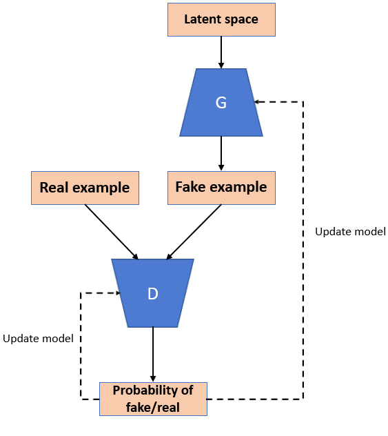
Recent advances in Deep Neural Networks, and in particular GANs (Generative Adversarial Networks) highlight the potential for a new approach for the automatic generation of maps. GAN is a framework proposed by Ian J. Goodfellow et al. [3] that is trained to generate data (images in most cases) with the same characteristics of a given training set. For example, a GAN trained on images of human faces would be able to generate realistic samples that are authentic to human observers.
The framework consists of two networks competing against each other, thus the term adversarial: a generative network, Generator , which creates fake data from a random distribution (usually normal or uniform) and a discriminative network, Discriminator , which, by giving it some data , estimates whether came from real data distribution or from the generator’s distribution .
A real world analogy would be the job of an art counterfeiter and a cop. The cop () learns to detect false paintings while the counterfeiter () improves on producing perfectly fake paintings indistinguishable from real ones.
The generation of images using GANs reached great success in recently years. Recent applications using this network include creation of realistic faces [4], pose guided person image generation [5] or transforming images from one domain to another [6].
Taking this into account, the research problem addressed in this work is to explore several GAN’s techniques in order to generate realistic and appealing maps for strategy games.
By “realistic”, we mean that maps should be perceived in a similar way to natural land formations. By “appealing”, we mean that maps should have suitable characteristics and elements discussed above, that allow players to have a more challenging and interesting experience.
Taking into account the research problem, if we have a proper and balanced heightmap’s dataset of natural landscapes, we believe that this type of technique can be successfully used to generate maps that resemble the original dataset, which will have the type of characteristics existing in natural landscapes, such as peninsulas and mountain ranges. Starting from a baseline GAN architecture, we will slowly improve its structure in order to achieve our goal, taking into account the proper evaluation of the models.
II Related Work
In this section we describe different types of GANs that appeared in recent works and that we will use.
II-A DCGAN
In the work of Alec Radford et al. [7] the authors managed to consolidate the junction of GAN and Convolutional Neural Network (CNN) frameworks, after several unsuccessfully attempts to do so in the past years.
CNN are a subset of neural networks most commonly applied to image and video recognition or computer vision problems. They were largely inspired by the visual cortex, small regions of cells sensitive to specific regions of the visual field [8]. These networks are mostly composed by convolutional layers, that are responsible for applying the convolution333In image processing, refers to the process of adding each pixel of the image to its local neighbors, weighted by a kernel. operation of the input using a filter, or kernel, and sending the result, also known as feature map to the next layer. If this kernel is designed to detect a specific type of feature on the input, then filtering it across the whole image would allow the kernel to detect that feature anywhere in the image independently of the feature’s location. By having this translation invariance characteristic and a shared-weight architecture, CNN are also known as Shift Invariant Artificial Neural Networks [9].
Their methodology consisted in adopting and modifying three demonstrated changes to CNN architectures:
-
1.
Replacing the pooling layers of the CNN baseline architecture for convolutional layers with stride 2 in order for and to learn its own spatial upsampling and downsampling respectively;
-
2.
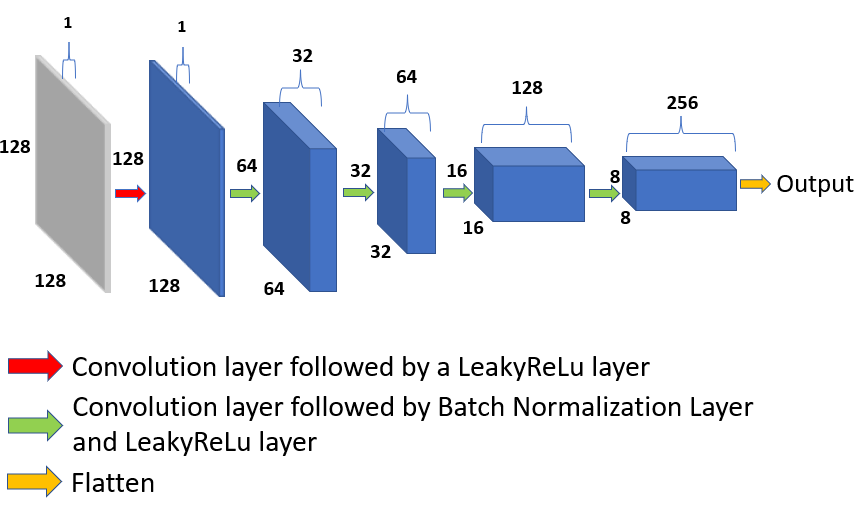
Elimination of fully connected layers for convolutional layers. To make the most use of these convolution layers, they added another layer at the beginning of that takes the input vector and reshapes it into a 4-dimensional tensor. They also added another layer at the end of that flattens the image to a single value output;
-
3.
Applying Batch Normalization to layers in order to stabilize learning by normalizing the input of a layer to have zero mean and unit variance, for each minibatch.
II-B Progressively Growing GANs
Generation of high-resolution images is a difficult task since it is easier to discriminate between the fake and real images. In the work of Karras et al. [4], the authors proposed a training methodology that consists on starting with low-resolution images, and then progressively increasing the resolution by adding layers to both the discriminator and generator (which are mirror images of each other and always grow in synchrony). In other words, the authors are slicing a bigger complex problem into smaller ones and slowly increasing the complexity to prevent the training from becoming unstable. The incremental addition of the layers allows the models to effectively learn coarse-level detail and later learn even finer detail, both on the generator’s and discriminator’s side.
The insertion of layers cannot be done directly due to sudden shocks to the already well-trained layers. Instead they phase in the layer. This operation consists on using a skip connection444Skip connections are connections of outputs from early layers to later layers through addition or concatenation to connect the new block to the input of or output of using a weighted sum with the existing input or output layer, that represents the influence of the new block. It is controlled by a parameter that starts at a very small value and increases linearly to 1 over the process of training. In other words, we can think of this operation as the layers slowly being inserted during the training phase.
In terms of results, this network was capable of generating high resolution images of , creating a high-resolution version of the CELEBA dataset [10].
II-C Wasserstein GAN
Martin Arjovsky et al. [11] propose a GAN that has an alternate way of training so that the generator model better approximates the distribution of data of a given dataset. More so, they present an alternate loss function in which is always giving enough information for the to improve himself, even if has reached its optimality.
The discriminator is replaced by a critic that instead of classifying an image as fake or real (in the interval [0,1]), it scores the fakeness or realness of an image (in the interval ],[). This score is also known as Wasserstein estimate. The critic is looking to estimate the Wasserstein distance between the dataset sample distribution and the generated images distribution, which corresponds to the distance between the average critic score on real and the average critic score on fake images. Thus the network’s objective function can be summarized as follows:
-
•
objective function is the difference between the average critic score on fake images and the average critic score on real images;
-
•
objective function is the average critic score on fake images.
Both the networks are trying to maximize these objective functions. Therefore, for , a larger score of the fake images will result in a higher output for the , encouraging to output higher scores for the fake images. For , a larger score for real images results in a lower value for the model, penalizing it, thus the encouragement for the critic to score lower scores for the real images.
II-D VAE + GAN
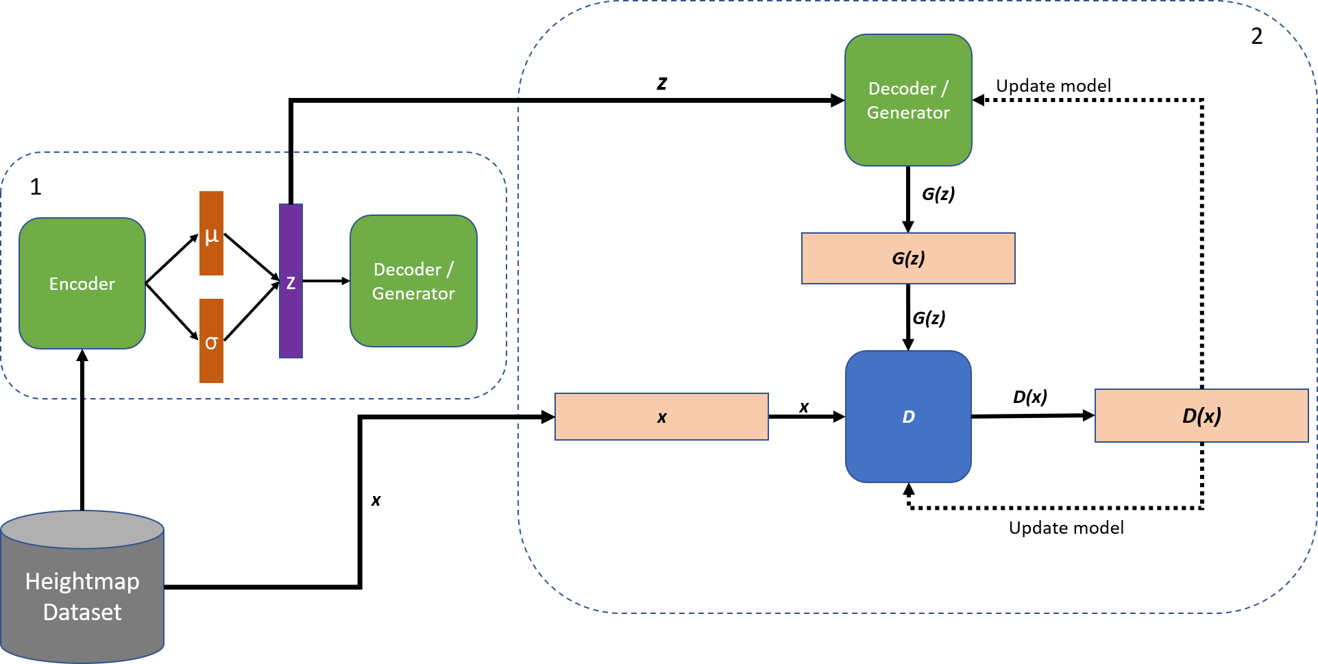
The idea of combining the power of Variational Autoencoders (VAE) and GAN was the basis for the work of Larsen et al. [12]. The motivation behind their work was to leverage learned representations to better measure similarities in the data distribution.
Autoencoders are another subset of neural networks used to generate images with good results. They learn a representation of a given data [13]. They are commonly used for face recognition or acquiring semantic meanings of words. The general idea behind this neural network is that they learn to copy the input to the output through a latent space that compresses the input maintaining only the most relevant and important information. The decoder then decompresses the information retained in the latent space ( also known as code) leading to a very similar copy of the output.
VAE are a subset of autoencoders specialized in content generation. They inherit the architecture from the traditional autoencoders but instead of mapping the input to a fixed latent space, the VAE maps the input onto a latent distribution, which allows us to take random samples from the latent space. These samples are then decoded using the decoder segment to generate outputs very similar to the inputs used to train the encoders. Instead of having a fixed vector as the latent space, the vector is replaced by two separate vectors, that represent the mean and the standard deviation of the distribution, respectively.
Typically, VAE uses element-wise similarity in their reconstruction error, however, Larsen et al. [12] propose using the GAN discriminator to measure the sample similarity. In other words, they use the GAN’s discriminator as a way to measure the difference between the VAE’s output and the original image.
The authors’ proposed architecture is comprised of a single model that simultaneously learns to encode, generate and compare samples from the dataset. The GAN’s generator coincides with the VAE’s decoder. The authors define the loss of the model as:
| (1) |
where is the Binary cross entropy loss and is defined as:
| (2) |
where is a prior regularization term, the Kullback-Leibler divergence and is the expected log likelihood (reconstruction error) expressed in the GAN discriminator:
| (3) |
with denoting a hidden representation of the th layer of the Discriminator.
III Dataset Creation
In order to apply the GAN-based techniques, it is necessary to have a group of examples of what the system is supposed to generate. Therefore, we began by building a proper dataset of natural landscapes which had the characteristics of the already existing land formations of the planet Earth, such as peninsulas and mountain ranges.
Data gathering
When looking for a proper dataset we had the idea that no data could resemble more the characteristics discussed in Section I than data from the real world, in which the terrain had already the desired complex elements and characteristics. Taking this idea into account, we used a public dataset 555https://www2.jpl.nasa.gov/srtm/cbanddataproducts.html with nearly global coverage of the planet Earth generated by a satellite radar topography mission. The dataset consists of several Digital Elevation Model (DEM) files created by a Ground Data Processing System supercomputer with a 3 arc-second sample spacing. We grouped the different DEM files together and exported them into a Tagged Image File Format using a program called Global Mapper, resulting in a Heightmap image with resolution, as shown on Fig 2.
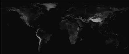
Preprocessing
As one can see in Fig 2 most regions of the Earth are a bit too dark making the terrain not very noticeable. This is not ideal for the techniques to be used since the altitude data should be more evenly distributed. In other words, we needed a higher range of pixel values so that their difference would be better distributed between and , instead of the original linear mapping between altitudes and pixel values. So, using the same program, we changed the image’s brightness level so that lower altitude regions could have higher pixel greyscale values.
We proceeded to crop the high resolution image into images with a sliding window of pixels, which gave in total images.
Dataset Augmentation / Removal of unwanted images
Due to the lacking of enough images on the dataset for a problem with a moderate level of complexity such as the one approached here, we had to perform dataset augmentation in order to increase the number of images. The procedure is described below:
-
1.
To the image, we applied different sets of image processing techniques: rotation between and degrees, and horizontal / vertical flipping. The rest of the image would then be filled with the pixel value .
-
2.
As done in the preprocessing phase, the was cropped into images with a sliding window of .
-
3.
Resulting images that had little to no continental land or were cut due to the image processing techniques, were removed. In other words, images that had of the pixel values , or had the pixel value of were removed.
This procedure was repeated times, ending up with images of resolution, which we found more than reasonable for the problem. Unfortunately, Working with -sized images would result in our models having a high number of parameters thus requiring more computational resources, such as memory, which we had not at our disposal. Therefore, we had to downsize the dataset to a resolution. The image rescaling was done using a nearest neighbor interpolation filter.
IV GANs’ Architecture and Training
Instead of just focusing on one type of GAN, we decided to explore several models in order to decide which one would be the most appropriate for the problem, making a comparison in terms of quality of the images generated, training efficiency and ease in training and convergence. We added tables which detail each model’s architecture in the Appendix.
IV-A DCGAN
The Deep Convolutional Generative Adversarial Network (DCGAN) architecture was the first to be tested, to serve as an initial baseline model and a foundation for the other models. We followed the majority of the architectural guidelines explained in [7] such as:
-
•
Using strided convolutions on and fractional-strided (transposed) convolutions on , allowing the network its own spatial downsampling and upsampling;
-
•
Batch Normalization layers in both networks, which helps the network on its learning process;
-
•
Removal of fully connected layers and replacing them with the convolutional layers except in the beginning of and in the end of ;
-
•
Leaky ReLU activation function for all layers of , since it is more effective for models generating images with higher resolution;
However, instead of applying the Rectified Linear Unit (ReLU) activation function to all layers of , we instead used the Leaky ReLU, since the latter activation function has been proven to be more effective than the ReLU [14].
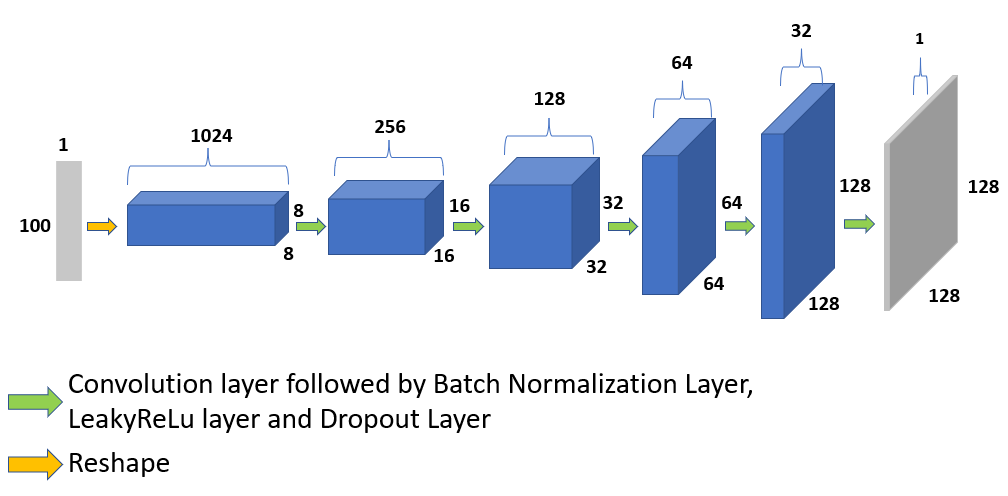
All of the convolutional and transposed convolution layers had a kernel size of , SAME padding and a stride of , except for the first convolution layer of which had stride of . Those layers’ weights were initialized using a zero mean normal distribution with standard deviation . The values used for the Batch Normalization, Leaky ReLU layers and the kernel size on both networks were the same as the ones used in [7].
It is well-known that GANs suffer from the vanishing gradient problem, where an optimal ( one that is really good at classifying the images as real and fake), doesn’t provide enough information for the to improve itself [11], [15].
Regarding the DCGAN’s training phase, in order to battle the GAN’s vanishing gradient problem we decided to add three hindering methods that would help in achieving this goal. These hindering methods, have the purpose of preventing from rapidly reaching a perfect discriminator scenario [16], [17], [15].
-
•
Adding a unique noise vector to each sample of the minibatch of real samples from and the minibatch of fake samples;
-
•
Applying One-sided Label Smoothing with .
-
•
Adding a Dropout layer after each Leaky ReLU layer on . For these layers we chose to set 50% of the input’s values to ;
We came up with three expressions for the . The first one illustrates an increasing over the number of epochs:
| (4) |
In the second and third one, the increases till half the number of epochs and then decreases.
| (5) |
| (6) |
In (5) the noise drops to half after half of the epochs have passed (e.g. - - - - …) while in (6) the noise ascends and descends at a same rate (e.g - - - - - …). We wanted to test what would happen if we hindered till half of the training phase and then ease it either by suddenly decreasing the to half at the middle of the training phase or having a similar rate for increasing and decreasing the .
IV-B WGAN
The second tested architecture was the Wasserstein Generative Adversarial Network (WGAN) discussed in Section II-C. With this model we were expecting to work on some of the problems that came with the DCGAN model such as the failure to converge and the vanishing gradient problems.
The structure of the generator from the DCGAN model and the WGAN model is exactly the same. The same goes for the discriminator from DCGAN model and the critic from WGAN model except we’re using a linear activation function as the last layer on the critic instead of the sigmoid, since the score for realness or fakeness of an image doesn’t have a limit value.
There are some things to be taken in consideration about the training phase:
-
•
As discussed in section II-C, during each epoch, is trained times more than ;
-
•
It was not to possible to implement the Wasserstein distance with the formulation presented in [11] using Keras’ API methods because Keras doesn’t allow a sum of losses from independent batches. We used the fact that maximizing the Wasserstein distance is equivalent to increasing the distance between the Wasserstein score for positive examples and the score for negative examples. One simple way of achieving this is by returning positive estimates for real examples and negative estimates for fake examples666https://machinelearningmastery.com/how-to-implement-wasserstein-loss-for-generative-adversarial-networks/.
-
•
When updating the weights, we clip them to stay in an interval between a constant and . This clipping is necessary to ensure the critic’s approximation to the Wasserstein distance, as explained in [11].
IV-C ProgGAN
For a third architecture we decided to apply the principles of the WGAN model and the idea of generating high-resolution images discussed in Section II-B together to create a GAN based on the Progressive Growing Generative Adversarial Network (ProgGAN). We wanted to verify if this technique would have interesting results in terms of training time optimization. We also wanted to see if it would generate images with higher resolution while maintaining a good quality.
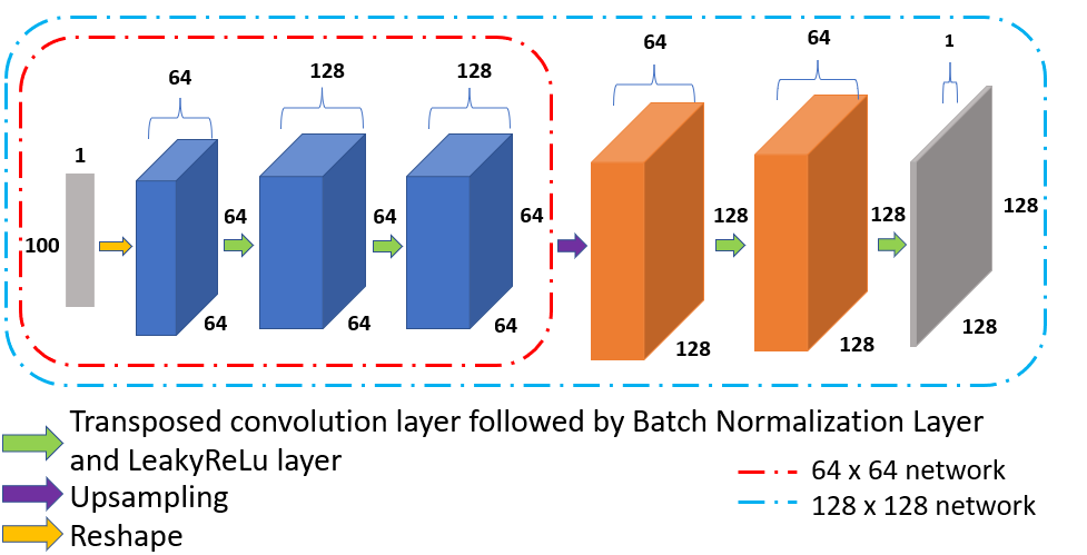
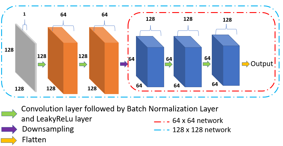
The upsampling layers use an upscaling factor of for both dimensions and a nearest neighbor interpolation. The downsampling layers perform an average pooling operation, using a downscaling factor of for both dimensions and a stride of . During training, the phasing in from giving full weight to the model (at the beginning of the training phase) to full weight to the model (end of the training phase) is done through a weighted sum layer controlling how much to weight the input from the and the models. It uses a parameter that grows linearly over the training phase.
Each of the models was trained separately, in this order: model growth model model. We treated each of the models as being a WGAN.
IV-D VAE + WGAN
As a final contribution, we wanted to combine the VAE and WGAN together. The idea was to train a VAE to encode and decode the images of our dataset of heightmaps. We hoped that using a generator that was already trained to create features from our dataset, such as in the VAE, would accelerate the WGAN’s training by increasing the efficiency in training time.
Fig. 7 depicts the model of the encoder.
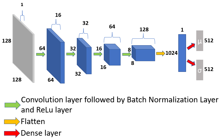
The decoder and the discriminator followed the same structure as the WGAN’s generator and critic. The only difference is that the last layer of the decoder uses a sigmoid activation function instead of the hyperbolic tangent used in WGAN’s generator.
In terms of training, we trained the VAE and WGAN separately. We started with the VAE, by just training the model for a fixed number of epochs. Then we took the decoder model of the VAE and used it as our WGAN’s generator. However, instead of normalizing our dataset between and for both the networks, we normalized it between and since the last activation function of the decoder is a sigmoid, which ranges between the latter values. For some of the experiments, instead of generating the from we generated them using the vectors and learned from the VAE. With this latter idea, we wanted to test if the decoder would be able to generate images with closer resemblance to the Heightmap dataset, since the vectors and contained features of that dataset.
V Results
All experiments were done in a desktop workstation with architecture x86_64, CPU AMD Ryzen 5 2600X Six-Core processor and one GeForce RTX 2080 Ti graphic cards with 11 GB RAM. For the implementation and training of the networks we used Keras777https://keras.io/, the version used was 2.3.1, a deep learning API running on top of Tensorflow888https://www.tensorflow.org/, the version used was 1.14.0. It provides abstractions and building blocks for developing and solving machine learning solutions.
V-A DCGAN
In terms of results, in the four experiments we performed, the networks were compiled using the Adam optimizer with learning rate and 999Exponential decay for the running average of the gradient. Both values were chosen as suggested in [7]. The networks were trained for 1000 Epochs. A brief description of every experiment made is described below:
-
•
E1: None of the discriminator hindering methods were used;
-
•
E2: All the discriminator hindering methods were implemented; Equation (4) for the noise vector;
-
•
E3: All the discriminator hindering methods were implemented; Equation (5) for the noise vector;
-
•
E4: All the discriminator hindering methods were implemented; Equation (6) for the noise vector;
In Fig. 9 one can observe the losses of and throughout the epochs for E1, and we can see the GAN’s vanishing gradient problem appearing.
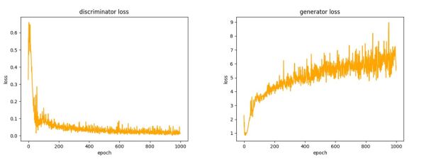
As we can observe, ’s loss rapidly converges to , while ’s loss keeps growing unsteadily. Early during the training phase, reaches its optimal state, which is perfectly discriminating between the real and fake images. Thus, is unable to improve, leading to a loss growth.
For E2, E3 and E4, despite the fact that the hindering methods above mentioned did in fact help battle the GAN’s vanishing gradient problem, the results obtained have a poor quality.
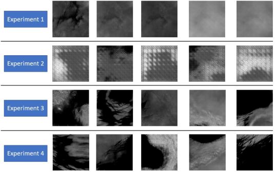
In E1, we can see that the model entered in a mode collapse, since the images generated have similar shapes, with some of them even having a blurry artifact. In E2 however, the quality of the images decayed, with the resulting images presenting some kind of artifacts in the form of a squared pattern. Experiments E3 and E4 yielded better results in terms of quality. Despite this results, all the images represented in Fig. 10 were classified as fake by the experiment’s respective discriminators.
V-B WGAN
The network was compiled using the RMSProp optimizer with learning rate of , as in [11]. In terms of results, we first ran some tests to see which value we should use as a constraint for clipping the weights values from this list of values: , , , , , . We ended up choosing as the constraint since it gave the best results in terms of the Wasserstein estimate.
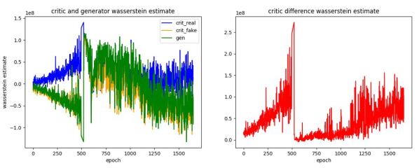
We ran a single but extensive experiment E5 where we trained the network for epochs with a training time of hours and minutes. Fig. 11 depicts the Wasserstein estimates of E5. The blue and yellow lines, which represent the Wasserstein estimate for the critic real and fake images, respectively, are distancing from each other. We can also verify this by looking at the other graphic, where the red line, which represents the difference between those two estimates, keeps growing troughout the training epochs.
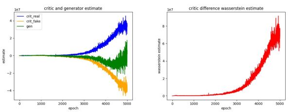
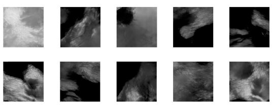
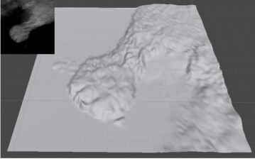
Fig. 12 depicts some of the images generated during the last epochs. The generator was able to reproduce realistic images with a relative good quality and level of detail. Some complex structures are also present such as peninsulas, mountain ranges and groups of islands. Fig. 13 depicts a 3D representation of a heightmap generated in E5, where we can see a peninsula and some small islands next to it.
Given the results we achieved with the previous experiment, we decided to run another experiment in order to check what type of results another WGAN, with a more complex structure and higher number of neurons than the previous one, could generate. So, in experiment E6 we trained the model presented in subsection IV-C for epochs, which took 217 hours of training time. Fig. 14 shows some of the images generated through some training epochs of E6. Using a WGAN with a more complex structure proved not to be so efficient, given that the images between experiments E5 and E6 have similar quality.
V-C ProgGAN
Taking into account the network structure and training algorithm previously discussed, we made one experiment regarding the ProgGAN model. To be able to verify the efficiency in training time we had to run an experiment E7 with similar amount of epochs to E6. Therefore, we trained the model for epochs ( epochs for each of the networks ).
Table I depict the training time for E6 and E7. As we can see, the ProgGAN model took less hours to train than the WGAN model.
| E6 | E7 | |
|---|---|---|
| 25h 3min | ||
| growth | 74h 9min | |
| 217h | 71h 10min | |
| TOTAL | 217h | 170h 23 min |
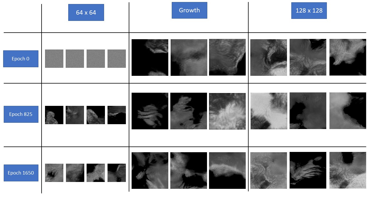
Fig 15, 16 and 17 depict the Wasserstein estimate of both generators and critics for the , growth and models, respectively.
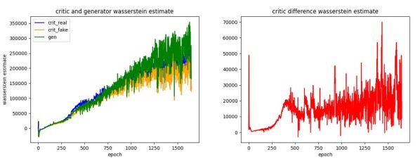
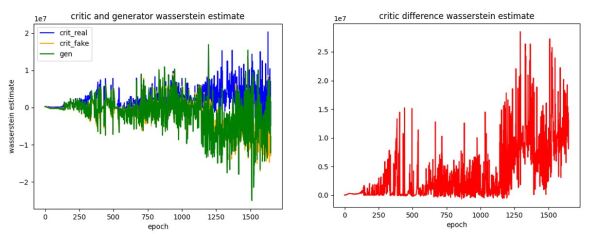
Despite the figures showing an erratic and unstable movement of the Wasserstein estimate during the training phase, we can see that in all of the models, the estimates of the real and fake images were moving away from each other, hence the line of the difference of the Wasserstein estimate on the critic going up.
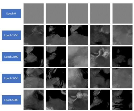
Fig. 18 shows some of the images generated through some training epochs of E7. We can see that the quality of the images from the model to the growth model and to the didn’t deteriorate. We can even say that the quality improved, since there is more variety of complex structures present in the end of the training phase such as bays, peninsulas, mountain ranges near the shore and islands.
V-D VAE + WGAN
We did several experiments with the VAE + WGAN architecture, to analyze factors such as:
-
•
Number of epochs needed to train the VAE in order for it to recreate the dataset images with a reasonable level of detail;
-
•
Generation of the random vector in order to be given as input to WGAN’s generator;
-
•
Comparison between training a WGAN with the decoder having already learned features from the Heightmap dataset and a WGAN without a pre-trained decoder.
Taking into account these factors the experiments are described as follow:
-
•
E8: VAE trained for epochs. Decoder with the weights already trained used as the WGAN’s generator. WGAN trained for more epochs, using a normal distribution with and for generating ;
-
•
E9: VAE trained for epochs. Decoder with the weights already trained used as the WGAN’s generator. WGAN trained for more epochs, using a normal distribution with and for generating ;
-
•
E10: Decoder, with the weights already trained in Experiment , used as the WGAN’s generator. WGAN trained for more epochs, using the vectors and learned from the VAE, for generating .
-
•
E11: WGAN trained for epochs to make a comparison between the models.
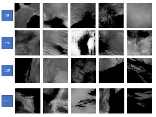
The training time for each experiment is denoted in Table II. As we can see, the difference between E9 or E10, which corresponds to training VAE for epochs and training the WGAN for epochs and E11 which corresponds to training the WGAN for epochs isn’t that big, saving at maximum minutes with the latter experiment. Fig. 23 below depicts images, for the several experiments, generated by the WGAN after training.
| Experiment | VAE | WGAN | Total |
|---|---|---|---|
| E8 | 8h 42 min | 7h 28 min | 16h 8 min |
| E9 | 1h 18 min | 7h 30 min | 8h 48 min |
| E10 | 1h 18 min | 7h 20 min | 8h 38 min |
| E11 | 8h 24 min | 8h 24 min |
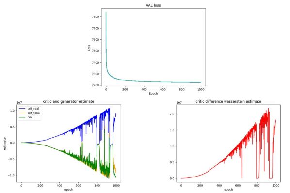
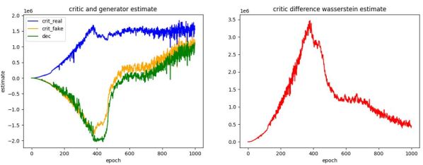
Regarding E8, the loss and estimates are shown in Fig. 19. The VAE’s training went well as expected, with its loss rapidly decreasing in the initial epochs, but stagnating around towards the end of the training. The WGAN’s training also went smoothly, despite some moments between the epochs and where all the estimates suddenly got close to each other.
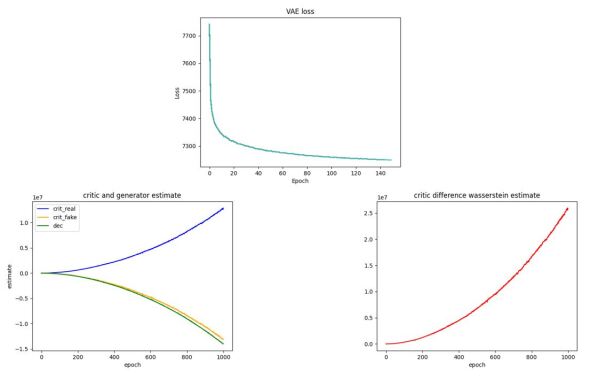
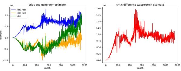
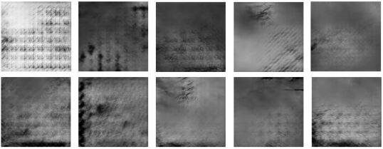
Since the stagnation of VAE’s loss happened early in its training phase we thought we could have trained it for a lower amount of epochs and still be able to generate images with good quality. Taking that into account, in E9, as shown in Fig. 20, we trained the VAE for only epochs. In this experiment, the WGAN training went really smoothly, as can be seen by the Wasserstein estimate graphic and the images generated. However, in this experiment, there were images, generated throughout the training process, that presented some strange artifacts as seen in Fig. 24. Even after the training was complete, some images with those kind of artifacts were generated.
In E10 we took the weights of the decoder trained in the VAE of the previous experiment and trained the WGAN for epochs again. However, we are using the vectors and learned from the VAE to generate our vectors , since they contain features of the Heightmap dataset. Fig. 21 and 23 depict the results of E10. The graphic of the Wasserstein estimate is not what we expected it to be. From epoch , the images generated by the decoder managed to fool the critic into thinking they were becoming more real throughout the remaining epochs, given that the Wasserstein estimate of the fake images went up after that epoch.
As the last experiment, we wanted to just train the WGAN for epochs, in order to make a proper comparison between the other experiments. Fig. 22 and 23 depict the results.
Discussion
The results obtained with the DCGAN were unsatisfying, as we were already expecting, due to several problems with this architecture already mentioned in the literature. The WGAN proved to be a good option since throughout the whole training phase the generator always had enough information provided by the critic to improve itself, thus ending up generating heightmaps with good quality. With the ProgGAN we saw that we could achieve the same results as in the WGAN with less training time. Curiously, the Wasserstein estimates did not follow the expected pattern. With the VAE + WGAN model, although it seemed to be a promising model in paper, we didn’t get quite the results we expected.
VI Conclusions
In this work, our purpose was to explore the GANs’ capabilities to generate images with high resolution and quality to try to create maps that look realistic and appealing for players, in a visual and even strategic way. That could not be done with the traditional approaches of PCG. Instead of just focusing on one model of the current state of the art of GANs we decided to explore several ones and test if they could indeed be used to generate such maps. We ended up exploring four models: DCGAN, WGAN, ProgGAN and VAE + WGAN, each one with its upsides and downsides. The DCGAN and VAE + WGAN models provided results with poor quality while the WGAN and ProgGAN models provided the best results, with the latter one being more efficient in terms of training time. Despite the poor results of the VAE + WGAN model, we think that this last model is one that should be further studied because its concept is promising.
Given the server memory limitations we were only able to work with images of resolution while the ideal scenario would be to work with an higher resolution such as . Further individual studies of each of these models or the ability to be able to expand these networks to images with higher resolution, given the proper hardware, are some examples of future work that could be explored and studied regarding this topic.
Acknowledgments
This work was supported by national funds through FCT, Fundação para a Ciência e a Tecnologia, under projects UIDB/04326/2020, UIDB/50021/2020, UIDP/04326/2020 and LA/P/0101/2020.
References
- [1] Ken Perlin “An Image Synthesizer” New York, NY, USA: Association for Computing Machinery, 1985, pp. 287–296
- [2] Xing Mei, Philippe Decaudin and Bao Gang Hu “Fast hydraulic erosion simulation and visualization on GPU” In Proceedings - Pacific Conference on Computer Graphics and Applications, 2007
- [3] Ian Goodfellow et al. “Generative adversarial networks” In arXiv, 2014
- [4] Tero Karras, Timo Aila, Samuli Laine and Jaakko Lehtinen “Progressive growing of GANs for improved quality, stability, and variation” In 6th International Conference on Learning Representations, ICLR 2018 - Conference Track Proceedings, 2018
- [5] Mehdi Mirza and Simon Osindero “Conditional Generative Adversarial Nets” In arXiv, 2014
- [6] Jun Yan Zhu, Taesung Park, Phillip Isola and Alexei A. Efros “Unpaired Image-to-Image Translation Using Cycle-Consistent Adversarial Networks”, 2017, pp. 2242–2251
- [7] Alec Radford, Luke Metz and Soumith Chintala “Unsupervised representation learning with deep convolutional generative adversarial networks” In arXiv, 2016
- [8] Ian Goodfellow, Yoshua Bengio and Aaron Courville “Learning deep architectures for AI” MIT Press, 2016
- [9] Wei Zhang, Kazuyoshi Itoh, Jun Tanida and Yoshiki Ichioka “Parallel distributed processing model with local space-invariant interconnections and its optical architecture” In Applied Optics, 1990
- [10] Ziwei Liu, Ping Luo and Xiaogang Wang Tang “Deep Learning Face Attributes in the Wild” In Proceedings of International Conference on Computer Vision (ICCV), 2015
- [11] Martin Arjovsky, Soumith Chintala and Léon Bottou “Wasserstein GAN” In arXiv, 2017
- [12] Anders Boesen Lindbo Larsen, Søren Kaae Sønderby, Hugo Larochelle and Ole Winther “Autoencoding beyond pixels using a learned similarity metric” In arXiv, 2016
- [13] Yoshua Bengio “Learning deep architectures for AI” Hanover, MA, USA: Now Publishers Inc., 2009
- [14] Andrew Gordon Wilson, Been Kim and William Herlands “Proceedings of NIPS 2016 Workshop on Interpretable Machine Learning for Complex Systems” In arXiv, 2016
- [15] Martin Arjovsky and Léon Bottou “Towards Principled Methods for Training Generative Adversarial Networks” In arXiv, 2017
- [16] Tim Salimans et al. “Improved techniques for training GANs” In arXiv, 2016
- [17] Phillip Isola, Jun-Yan Zhu, Tinghui Zhou and Alexei A. Efros “Image-to-Image Translation with Conditional Adversarial Networks” In arXiv, 2018
- ANN
- Artificial Neural Networks
- BN
- Batch Normalization
- CNN
- Convolutional Neural Networks
- DCGAN
- Deep Convolutional Generative Adversarial Network
- DEM
- Digital Elevation Model
- GAN
- Generative Adversarial Networks
- IST
- Instituto Superior Tecnico
- PCG
- Procedural Content Generation
- ProgGAN
- Progressive Growing Generative Adversarial Network
- ReLU
- Rectified Linear Unit
- SRTM
- Shuttle Radar Topography Mission
- VAE
- Variational Autoencoder
- WGAN
- Wasserstein Generative Adversarial Network
Appendix A
In this appendix we show the detailed architecture of the implemented models and the hyper-parameters used, to allow for reproducibility of the results. For the DCGAN network, we used the Adam Optimizer with learning rate 0.0002 and = 0.5. For the WGAN and ProgGAN network, we used the RMSProp optimizer with learning rate 0.0005. For the VAE + WGAN model we trained the VAE and then the whole model, using the RMSProp optimizer with learning rate 0.0003 and 0.0005, respectively.
| Layer name | Act. | Input shape | Output shape |
|---|---|---|---|
| Dense | - | ||
| Reshape | - | ||
| Deconv | - | ||
| BatchNorm | - | ||
| LeakyReLU | LeakyReLU | ||
| Dropout | - | ||
| Deconv | - | ||
| BatchNorm | - | ||
| LeakyReLU | LeakyReLU | ||
| Dropout | - | ||
| Deconv | - | ||
| BatchNorm | - | ||
| LeakyReLU | LeakyReLU | ||
| Dropout | - | ||
| Deconv | - | ||
| BatchNorm | - | ||
| LeakyReLU | LeakyReLU | ||
| Dropout | - | ||
| Deconv | tanh |
| Layer name | Act. | Input shape | Output shape |
|---|---|---|---|
| Conv | - | ||
| LeakyReLU | LeakyReLU | ||
| Conv | - | ||
| BatchNorm | - | ||
| LeakyReLU | LeakyReLU | ||
| Conv | - | ||
| BatchNorm | - | ||
| LeakyReLU | LeakyReLU | ||
| Conv | - | ||
| BatchNorm | - | ||
| LeakyReLU | LeakyReLU | ||
| Conv | - | ||
| BatchNorm | - | ||
| LeakyReLU | LeakyReLU | ||
| Flatten | - | ||
| Dense | sigmoid |
| Layer name | Act. | Output shape | |
|---|---|---|---|
| Deconv | - | ||
| BatchNorm | - | ||
| LeakyReLU | LeakyReLU | ||
| Deconv | - | ||
| BatchNorm | - | ||
| LeakyReLU | LeakyReLU | ||
| UpSampling | - | ||
| Deconv | - | ||
| BatchNorm | - | ||
| LeakyReLU | LeakyReLU | ||
| Deconv | - | ||
| BatchNorm | - | ||
| LeakyReLU | LeakyReLU | ||
| Conv | - | ||
| BatchNorm | - | ||
| LeakyReLU | LeakyReLU | ||
| Conv | - | ||
| BatchNorm | - | ||
| LeakyReLU | LeakyReLU | ||
| Downsample | - | ||
| Conv | - | ||
| BatchNorm | - | ||
| LeakyReLU | LeakyReLU | ||
| Conv | - | ||
| BatchNorm | - | ||
| LeakyReLU | LeakyReLU |
| Layer name | Act. | Input shape | Output shape |
|---|---|---|---|
| Dense | - | ||
| Reshape | - | ||
| Deconv | Tanh | ||
| Layer name | Act. | Input shape | Output shape |
|---|---|---|---|
| Conv | - | ||
| LeakyReLU | LeakyReLU | ||
| Flatten | - | ||
| Dense | linear | ||
| Layer name | Act. | Input shape | Output shape |
|---|---|---|---|
| Dense | - | ||
| Reshape | - | ||
| Deconv | Tanh | ||
| Layer name | Act. | Input shape | Output shape |
|---|---|---|---|
| Conv | - | ||
| LeakyReLU | LeakyReLU | ||
| Flatten | - | ||
| Dense | linear | ||
| Layer name | Act. | Input shape | Output shape |
|---|---|---|---|
| Conv | - | ||
| BatchNorm | - | ||
| ReLU | ReLU | ||
| Conv | - | ||
| BatchNorm | - | ||
| ReLU | ReLU | ||
| Conv | - | ||
| BatchNorm | - | ||
| ReLU | ReLU | ||
| Conv | - | ||
| BatchNorm | - | ||
| ReLU | ReLU | ||
| Flatten | - | ||
| Dense | - | ||
| BatchNorm | - | ||
| ReLU | ReLU | ||
| (Dense) | - | ||
| (Dense) | - |