ExcelFormer: A Neural Network Surpassing GBDTs on Tabular Data

Abstract

Though deep neural networks have gained enormous successes in various fields (e.g., computer vision) with supervised learning, they have so far been still trailing after the performances of GBDTs on tabular data. Delving into this task, we determine that a judicious handling of feature interactions and feature representation is crucial to the effectiveness of neural networks on tabular data. We develop a novel neural network called ExcelFormer, which alternates in turn between two attention modules that shrewdly manipulate feature interactions and feature representation updates, respectively. A bespoke training methodology is jointly introduced to facilitate model performances. Specifically, by initializing parameters with minuscule values, these attention modules are attenuated when the training begins, and the effects of feature interactions and representation updates grow progressively up to optimum levels under the guidance of our proposed specific regularization schemes Feat-Mix and Hidden-Mix as the training proceeds. Experiments on 28 public tabular datasets show that our ExcelFormer approach is superior to extensively-tuned GBDTs, which is an unprecedented progress of deep neural networks on supervised tabular learning. The codes are available at https://github.com/WhatAShot/ExcelFormer.

1 Introduction

Neural networks have been firmly established as state-of-the-art approaches in various fields such as computer vision (Srivastava et al., 2015; Khan et al., 2022), natural language processing (Hochreiter & Schmidhuber, 1997; Vaswani et al., 2017), and automatic speech recognition (Dong et al., 2018). However, on tabular data, one of the most ubiquitous data formats, neural networks have not yet achieved comparable performances as traditional gradient boosting decision trees (GBDTs) (Chen & Guestrin, 2016; Prokhorenkova et al., 2018; Duan et al., 2020) in supervised learning despite numerous efforts (Borisov et al., 2021). This hinders the widespread adoption of neural networks and progress towards general artificial intelligence applications.

It has been suggested (Grinsztajn et al., 2022) that three inherent characteristics of tabular data impeded the performances of known neural networks: irregular patterns of the target function, negative effects of uninformative features, and non-rotationally-invariant features. Based on these propositions, we identify two keys for largely promoting the capabilities of neural networks on tabular data:

(i) An appropriate feature representation learning approach. Though it was demonstrated (Rahaman et al., 2019) that neural networks could likely predict overly smooth solutions on tabular data, a deep learning (DL) model was also observed to be capable of memorizing random labels (Zhang et al., 2021). To deal with irregular target function patterns (Gorishniy et al., 2021) and spurious correlations of targets and features in tabular data, an appropriate organization of feature representation is needed to well fit the irregular patterns while maintaining generalizability.

(ii) An effective feature interaction approach. Since features of tabular data are non-rotationally-invariant and a considerable portion of data is uninformative, network generalization can be harmed when a model incorporates useless feature interactions. But, theoretical analysis (Ng, 2004) suggested that known neural networks are naturally ineffective in dealing with data that have very limited relevant features, incurring a cost of high worst-case sample complexity. Thus, an effective interaction approach is needed to prevent negative effects of ill-suited feature interactions.

Some previous studies designed feature embedding approaches (Gorishniy et al., 2022) to alleviate overly smooth solutions inspired by (Tancik et al., 2020), or employed regularization (Katzir et al., 2020) and shallow models (Cheng et al., 2016) to promote model generalization. While some neural networks utilized sophisticated feature interaction approaches (Yan et al., 2023; Chen et al., 2022; Gorishniy et al., 2021) for better selective feature interactions. Although these tailored designs gained performances on supervised tabular data tasks, their performances are still not comparable with GBDT approaches (e.g., XGboost) on a diverse array of datasets (Borisov et al., 2021).

Our work pushes this research envelop: We develop a new neural network that, for the first time, outperforms GBDTs on a wide range of public tabular datasets. This is achieved based on the cooperation of a new tabular data tailored architecture called ExcelFormer and a bespoke training methodology, which jointly learns appropriate feature representation update functions and judicious feature interactions (satisfying aforementioned (i) and (ii)). For better feature representations, we propose an attention module, called attentive intra-feature update module (AiuM), which is more powerful than previous non-attentive representation update approaches (e.g., linear or non-linear projection networks). For feature interactions, we present a conservative approach based on a novel module called directed inter-feature attention module (DiaM), which avoids compromising the semantics of critical features by only allowing features of lower importance to fetch information from those of higher importance. Our ExcelFormer is mainly built by stacking alternately these two types of modules in turn.

Since the main ingredients AiuM and DiaM are both flexible attention based modules, our training methodology aims to prevent ExcelFormer from converging to an overly complicated representation function that overfits irregular target functions and from introducing useless feature interactions to hurt generalization. At the start of training, a novel initialization approach assigns minuscule values to the weights of DiaM and AiuM, so as to attenuate the intra-feature representation updates and inter-feature interactions. During training, the effects of DiaM and AiuM then grow progressively to optimum levels under the guidance of our new regularization schemes Feat-Mix and Hidden-Mix. Hidden-Mix and Feat-Mix are two variants of Mixup (Zhang et al., 2018) specifically for tabular data, which avoid the disadvantages of the original Mixup approach (to be discussed in Sec. 4) and respectively prioritize to promote the learning of feature representations and feature interactions.

Our main contributions are summarized as follows.

• We present the first neural network that outperforms GBDTs (e.g., XGboost), which is verified by comprehensive experiments on 28 public tabular datasets.

• We identify two key capabilities of neural networks for effectively handling tabular data, which will inspire further researches.

• To equip our ExcelFormer model with the two key capabilities, we develop new modules and a novel training methodology that cooperatively promote the model’s effectiveness.

• We propose two tabular-data-specific Mixup variants, Hidden-Mix and Feat-Mix, which are superior to the vanilla input Mixup approach on tabular data.

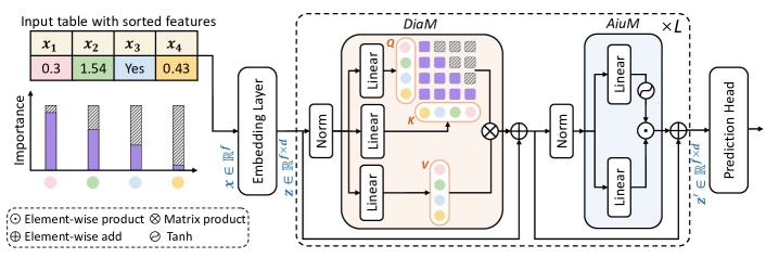
Figure 1: Illustrating our proposed ExcelFormer model. AiuM and DiaM denote the attentive intra-feature update module and directed inter-feature attention module, respectively. “Norm” denotes a LayerNorm layer (Ba et al., 2016). Before being fed into the model, the input features are sorted according to a feature importance metric (e.g., mutual information).

2 Related Work

Supervised Tabular Learning.

Since neural networks have been demonstrated to be efficient on various data types (e.g., images (Khan et al., 2022)), plentiful efforts were made to harness the power of neural networks on tabular data. However, so far GBDT approaches (e.g., XGboost) still remain as the go-to choice (Katzir et al., 2020) for various supervised tabular tasks (Borisov et al., 2021; Grinsztajn et al., 2022), due to their superior performances on diverse tabular datasets. To achieve GBDT-level results, recent studies focused on devising sophisticated neural modules for heterogeneous feature interactions (Gorishniy et al., 2021; Chen et al., 2022; Yan et al., 2023), mimicking tree-like approaches (Katzir et al., 2020; Popov et al., 2019; Arik & Pfister, 2021) to find decision paths, or resorting to conventional approaches (Cheng et al., 2016; Guo et al., 2017). Apart from model designs, various data representation approaches, such as feature embedding (Gorishniy et al., 2022; Chen et al., 2023), discretization of continuous features (Guo et al., 2021; Wang et al., 2020), and Boolean algebra based methods (Wang et al., 2021), were applied to deal with irregular target patterns (Tancik et al., 2020; Grinsztajn et al., 2022). These attempts suggested the potentials of neural networks, but still yielded inferior performances comparing with GBDTs on a wide range of tabular datasets. Several challenges for neural networks on tabular data were summed up in (Grinsztajn et al., 2022). But no solution has been given, and these challenges still remain open. Besides, there were some attempts (Wang & Sun, 2022; Arik & Pfister, 2021; Yoon et al., 2020) to apply self-supervision to tabular datasets. However, these approaches are dataset- or domain-specific, and appear difficult to be adopted widely due to the heterogeneity of tabular datasets.

Mixup and Its Variants.

The original Mixup (Zhang et al., 2018) generates a new data by convex interpolations of two given data, which was proved beneficial on various image datasets (Tajbakhsh et al., 2020; Touvron et al., 2021a) and some tabular datasets. However, we found that the original Mixup may conflict with irregular target patterns (to be discussed in Sec. 4) and hardly cooperate with the cutting-edge models (Gorishniy et al., 2021; Somepalli et al., 2021). ManifoldMix (Verma et al., 2019) and Flow-Mixup (Chen et al., 2020) applied convex interpolations to the hidden states, which did not fundamentally alter the way to synthesize new data and exhibited similar characteristics as the vanilla input Mixup. The follow-up variants CutMix (Yun et al., 2019), AttentiveMix (Walawalkar et al., 2020), SaliencyMix (Uddin et al., 2020), ResizeMix (Qin et al., 2020), and PuzzleMix (Kim et al., 2020) spliced two images spatially, which defended local patterns of images but are not directly available to tabular data. Darabi et al (Darabi et al., 2021) and Gowthami et al (Somepalli et al., 2021) applied Mixup and CutMix-like approaches in tabular data pre-training. It was shown (Kadra et al., 2021) that a search through regularization approaches could promote the performance of a simple neural network up to the XGboost level. But, time-consuming hyper-parameter tuning is a necessity in their settings, while XGboost and Catboost may not be extensively tuned. In contrast, our ExcelFormer models with fixed settings achieve GBDT-level performances without hyper-parameter tuning.

3 ExcelFormer

3.1 The Overall Architecture

Fig. 1 shows our proposed ExcelFormer model. ExcelFormer is built mainly based on two simple ingredients, the attentive intra-feature update module (AiuM) and directed inter-feature attention module (DiaM), which respectively conduct feature representation update and feature interactions. During the processing, $f$ features of an input data $x\in\mathbb{R}^{f}$ are first tokenized by a neural embedding layer into representations of size $d$ each, denoted as $z^{(0)}\in\mathbb{R}^{f\times d}$. It is then successively processed by $L$ DiaMs and $L$ AiuMs alternately. These two modules both have a LayerNorm head, and are accompanied with additive shortcut connections as illustrated in Fig. 1. Finally, a probability vector of $C$ categories $p\in\mathbb{R}^{C}$ ($C>2$) for multi-class classification or a scale value $p\in\mathbb{R}^{1}$ for regression and binary classification is produced by a prediction head.

3.2 Attentive Intra-feature Update Module (AiuM)

A possible conflict between the irregularity of target functions and over-smooth solutions produced by neural networks was identified (Grinsztajn et al., 2022). In known Transformer-like models (Yan et al., 2023; Gorishniy et al., 2021), the commonly-used position-wise feed-forward network (FFN) (Vaswani et al., 2017) was employed for feature representation update. However, we empirically discovered that the FFN containing two linear projections and a ReLU activation is not flexible enough to fit irregular target functions, and hence design an attention approach to handle intra-feature representation updates, by:

$$z^{\prime}=\tanh{(zW^{(l)}_{1}+b^{(l)}_{1})}\odot(zW^{(l)}_{2}+b^{(l)}_{2}),$$ (1)

where $W^{(l)}_{1}\in\mathbb{R}^{d\times d}$, $W^{(l)}_{2}\in\mathbb{R}^{d\times d}$, $b^{(l)}_{1}\in\mathbb{R}^{d}$, and $b^{(l)}_{2}\in\mathbb{R}^{d}$ are all learnable parameters for the $l$-th layer, $\odot$ denotes element-wise product, and $z$ and $z^{\prime}$ denote the input and output representations, respectively. Our experiments show that Eq. (1) is more powerful than FFN with the same computational costs. Notably, the operations in Eq. (1) do not conduct any feature interactions.

3.3 Directed Inter-feature Attention Module (DiaM)

It was pointed out (Ng, 2004) that neural networks are inherently inefficient to organize feature interactions, yet previous work empirically demonstrated the benefits of feature interactions (Chen et al., 2022; Cheng et al., 2016). Thus, we present a conservative approach for feature interactions that allows only the lower target-relevant features to gain access to the information of the higher target-relevant features. Before feeding features into ExcelFormer, we sort them in descending order according to the feature importance (we use mutual information in this paper) with respect to the targets in the training set. For judiciously handling feature interactions, we perform a special self-attention operation with an unoptimizable mask $M$, as:

$$z^{\prime}=\sigma(((zW_{q})(zW_{k})^{T}\oplus M)/\sqrt{d})(zW_{v}),$$ (2)

where $W_{q},W_{k}$, $W_{v}\in\mathbb{R}^{d\times d}$ are all learnable matrices, $\oplus$ is element-wise addition, and $\sigma$ is the softmax operating along the last dimension. The elements in the lower triangle portion of $M\in\mathbb{R}^{f\times f}$ are all set to zeros, and the remaining elements of $M$ are all set as negative infinity (using $-10^{5}$ in our implementation as default). This makes the elements in the upper triangle portion (except for the diagonal elements) of the attention map all zeros after softmax activation. In practice, Eq. (2) is extended to a multi-head self-attention version, with 32 heads by default.

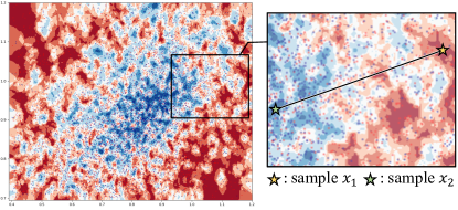
Figure 2: Decision boundaries of $k$-Nearest Neighbors ($k$NN, $k=8$) for the 2 most important features (by mutual information) of a zoomed-in part of the Higgs dataset. The convex combinations (points on the black line) of two samples $x_{1}$ and $x_{2}$ of two different categories likely are in conflict with the irregular target function.

Remarks. By our DiaM, a feature is updated by features of higher importance, but not vice versa. This remains as the interactions of any two features while protecting important features to a large extent if some interactions performed by the model are ill-suited. Our DiaM might appear similar to some self-attention mechanisms (Radford et al., 2018). But, a distinguishing aspect of our method is that the process is applied with feature importance (features are sorted in descending order based on the feature importance). Mutual information is used for feature importance in this paper.

3.4 Embedding Layer

Our embedding layer is also an attention based module that is similar to AiuM. In Eq. (1), the parameters $W_{1}$, $W_{2}$, $b_{1}$, and $b_{2}$ are shared among features, while in the embedding layer, the parameters are not shared among features, as:

$$z^{(0)}=\tanh{(x\odot W^{(0)}_{1}+b^{(0)}_{1})}\odot(x\odot W^{(0)}_{2}+b^{(0)}_{2}),$$ (3)

where the input features $x\in\mathbb{R}^{f}$, the learnable parameters $W^{(0)}_{1},W^{(0)}_{2}\in\mathbb{R}^{f\times d}$, $b^{(0)}_{1},b^{(0)}_{2}\in\mathbb{R}^{f\times d}$, and $\odot$ is element-wise product. Before being fed to the embedding layer, numerical features are normalized and categorical features are transformed into numerical features by the CatBoost Encoder implemented with the Sklearn Python package. 

3.5 Prediction Head

In our ExcelFormer, we do not use a class token in target function prediction as in previous Transformer-based approaches for tabular data (Gorishniy et al., 2021), since it was proved inefficient for feature interactions that were also conducted by class token based approaches. Our prediction head is directly applied to the output of the last AiuM, which contains two linear projection layers to separately compress the information along the feature dimension and the representation dimension, by:

$$p=\phi(W_{d}(\text{PReLU}((z^{(L)})^{T}W_{f}+b_{f}))^{T}+b_{d}),$$ (4)

where $z^{(L)}$ is the output of the top-most AiuM, $W_{f}\in\mathbb{R}^{f\times C}$ and $b_{f}\in\mathbb{R}^{C}$ ($C$ is the target category count in multi-classification for $C>2$; $C=1$ for regression and binary classification) compress the features, and $W_{d}\in\mathbb{R}^{d\times 1}$ and $b_{d}\in\mathbb{R}^{1}$ jointly compress the representation size $d$ into 1. $\phi$ is sigmoid for $C=1$, and is softmax for $C>2$.

4 Training Methodology

Our proposed AiuM and DiaM satisfy both the two keys (i) and (ii) given in Sec. 1 respectively. Further, we argue that their effectiveness can be improved by using tailored training methodology since vanilla neural network training strategies were considered inefficient for tabular data (Ng, 2004; Rahaman et al., 2019). Mixup (Zhang et al., 2018) is one of the most effective regularization approaches for neural networks, but our tests showed that it cannot well cooperate with some cutting-edge approaches like (Gorishniy et al., 2021; Somepalli et al., 2021). Besides, such element-wise convex interpolation operations are intuitively in conflict with irregular target functions of tabular datasets. Fig. 2 shows an example of an irregular target function of tabular data, and obviously the data synthesized by the original Mixup (i.e., convex combination) conflict with the target function. To address this issue, we introduce two Mixup variants, Hidden-Mix and Feat-Mix, for tabular data, which can enhance the model performances and avoid the conflicts shown in Fig. 2. Besides, we propose an attenuated initialization approach for these two modules. For easier understanding, we first introduce Hidden-Mix and Feat-Mix, and then the attenuated initialization approach.

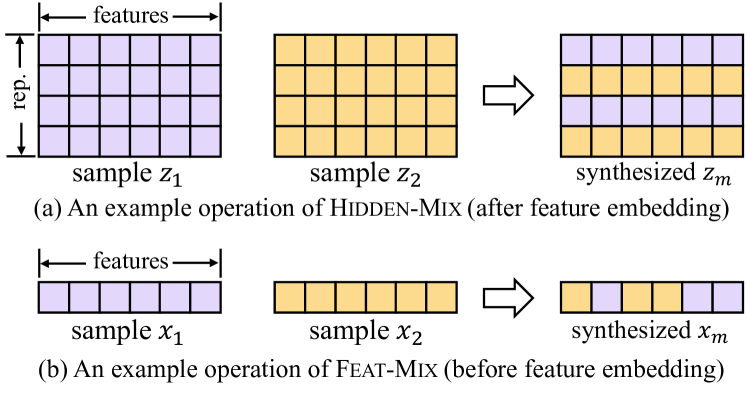
Figure 3: Examples for the Hidden-Mix and Feat-Mix operations, where “rep.” means “representations”.

4.1 Hidden-Mix

Our Hidden-Mix is applied to the representations after the embedding layer and the labels. It exchanges some representation elements of two samples (e.g., Fig. 3), by:

$$\left\{\begin{aligned} &z_{\text{m}}^{(0)}=S_{H}\odot z_{1}^{(0)}+(\mathbbm{1}_{H}-S_{H})\odot z_{2}^{(0)},\\ &y_{\text{m}}=\lambda_{H}y_{1}+(1-\lambda_{H})y_{2},\end{aligned}\right.$$ (5)

where $z_{1}^{(0)},z_{2}^{(0)},z_{\text{m}}^{(0)}\in\mathbb{R}^{f\times d}$ are the feature representations of two samples and the synthesized sample, and $y_{1},y_{2},y_{\text{m}}$ are the labels of the two samples and synthesized sample. The coefficient matrix $S_{H}$ and the all-one matrix $\mathbbm{1}_{H}$ are of size $f\times d$. $S_{H}=[s_{1},s_{2},\ldots,s_{f}]^{T}$, all whose vector $s_{h}\in\mathbb{R}^{d}$ ($h=1,2,\ldots,f$) are identical and have $\lfloor\lambda_{H}\times d\rfloor$ randomly selected elements of 1’s and the rest elements are 0’s. Similar to vanilla input Mixup (Zhang et al., 2018), the scalar coefficient $\lambda_{H}$ is sampled from the $\mathcal{B}eta(\alpha_{H},\alpha_{H})$ distribution, where $\alpha_{H}$ is a hyper-parameter.

Interpretation. Our Hidden-Mix encourages learning linear feature representation solutions. Consider a simple situation in which there are two data (after embedding layer), $z_{a}\in\mathbb{R}^{f\times d}$ and $z_{b}\in\mathbb{R}^{f\times d}$, the number of feature $f=1$, representation dimension $d=2$, and $\lambda_{H}=\frac{1}{2}$, then we have $y_{\text{m}}=\frac{1}{2}(y_{a}+y_{b})$ ($y_{a}$ and $y_{b}$ are labels of $a$ and $b$, and $y_{\text{m}}$ is the label of synthesized data). Thus, we can infer the constraint as a neural network $\mathbf{g}$ that $\mathbf{g}(z_{a}[0,0],z_{b}[0,1])+\mathbf{g}(z_{b}[0,0],z_{a}[0,1])=\mathbf{g}(z_{a}[0,0],z_{a}[0,1])+\mathbf{g}(z_{b}[0,0],z_{b}[0,1])$, in which the index $[i,j]$ indicates the $j$-th representation element of the $i$-th feature. For a simple neural network $\mathbf{g}(z[0,0],z[0,1])=w^{\mathbf{g}}_{1}z[0,0]+w^{\mathbf{g}}_{2}z[0,1]+w^{\mathbf{g}}_{3}z[0,0]z[0,1]$, it is obvious that Hidden-Mix requires $w^{\mathbf{g}}_{3}(z_{a}[0,0]z_{b}[0,1]+z_{a}[0,1]z_{b}[0,0])\equiv w^{\mathbf{g}}_{3}(z_{a}[0,0]z_{a}[0,1]+z_{b}[0,0]z_{b}[0,1])$ for any $z_{a}$ and $z_{b}$, and thus $w^{\mathbf{g}}_{3}=0$. In our ExcelFormer, AiuM and the embedding layer are implemented with flexible attention operations for fitting irregular target functions, while our Hidden-Mix prioritizes to learn a linear representation update approach for a feature and avoid over-fitting.

4.2 Feat-Mix

See the examples in Fig. 3. Unlike Hidden-Mix acting on the representation dimension, our Feat-Mix swaps parts of features between two input samples $x_{1},x_{2}\in\mathbb{R}^{f}$ (following the input Mixup (Zhang et al., 2018)), by:

$$\left\{\begin{aligned} &x_{\text{m}}=\mathbf{s}_{F}\odot x_{1}+(\mathbbm{1}_{F}-\mathbf{s}_{F})\odot x_{2},\\ &y_{\text{m}}=\Lambda y_{1}+(1-\Lambda)y_{2},\end{aligned}\right.$$ (6)

where the vector $\mathbf{s}_{F}$ and the all-one vector $\mathbbm{1}_{F}$ are of size $f$, $\mathbf{s}_{F}$ contains $\lfloor\lambda_{F}\times f\rfloor$ randomly chosen 1’s and the rest of its elements are 0’s ($\lambda_{F}\sim\mathcal{B}eta(\alpha_{F},\alpha_{F})$), and $y_{1}$, $y_{2}$, and $y_{m}$ are labels of samples $x_{1}$, $x_{2}$, and the synthesized sample. $\Lambda$ is the normalized sum of the mutual information of the features selected by $\mathbf{s}_{F}$, which is computed by:

$$\Lambda=\nicefrac{{\sum_{\mathbf{s}_{F}^{(i)}=1}\text{MI}^{(i)}}}{{\sum^{f}_{i=1}\text{MI}^{(i)}}},$$ (7)

where $\mathbf{s}_{F}^{(i)}$ is the $i$-th element of $\mathbf{s}_{F}$, and $\text{MI}^{(i)}$ is the mutual information of the $i$-th feature.

Interpretation. Consider two tabular data $x_{a}$ and $x_{b}$ before being processed by the embedding layer (with $f=2$, the sampled $\lambda_{F}=0.5$, and $\text{MI}^{(1)}=\text{MI}^{(2)}$) that are processed by Feat-Mix. One can easily infer the constraint as a neural network $\mathbf{h}$ such that $\mathbf{h}(x_{a}[0],x_{b}[1])+\mathbf{h}(x_{b}[0],x_{a}[1])=\mathbf{h}(x_{a}[0],x_{a}[1])+\mathbf{h}(x_{b}[0],x_{b}[1])$, in which $x[i]$ indicates the $i$-th feature value of the data $x$. For a neural network $\mathbf{h}(x[0],x[1])=w^{\mathbf{h}}_{1}x[0]+w^{\mathbf{h}}_{2}x[1]+w^{\mathbf{h}}_{3}x[0]x[1]$, it is suggested that $w^{\mathbf{h}}_{3}$ is likely to be 0 and Feat-Mix is disposed to make the neural network $\mathbf{h}$ learn a non-feature-interaction function. It encourages DiaM to include solely necessary interactions, discarding the useless ones.

4.3 An Attenuated Initialization

The function of our proposed attenuated initialization approach aims to reduce the effects of DiaM and AiuM during the start of the model training. This initialization approach is built upon the commonly used He’s initialization (He et al., 2015) or Xavier initialization (Glorot & Bengio, 2010) approaches, by rescaling the variance of an initialized weight $w$ with $\gamma$ ($\gamma\rightarrow 0^{+}$) while keeping the expectation at 0:

$$\text{Var}(w)=\gamma\text{Var}_{\text{prev}}(w),$$ (8)

where $\text{Var}_{\text{prev}}(w)$ denotes the weight variance used in the previous work (He et al., 2015; Glorot & Bengio, 2010). In this work, we set $\gamma=10^{-4}$. To reduce the impacts of AiuM and DiaM, we can either apply Eq. (8) to all the parameters of these modules or to part of them. We empirically witness that these options all perform similarly. We apply Eq. (8) to all the parameters in AiuM and in DiaM as default. Thus, these two modules have almost no effects before training.

Table 1: Performance comparison of various ExcelFormer versions with extensively tuned XGboost and Catboost on 28 public datasets. The performances of ExcelFormers that outperform both XGboost and Catboost are marked in bold, while those that outperform either XGboost or Catboost are underlined. The performances of XGboost and Catboost are bold if they are the best results.

Datasets AN IS CP VI YP GE CH SU BA BR XGboost -0.1076 95.78 -2.1370 -0.1140 -0.0275 68.75 85.66 -0.0177 88.97 -0.0769 Catboost -0.0929 95.26 -2.5160 -0.1181 -0.0275 66.54 86.62 -0.0220 89.16 -0.0931 ExcelFormer-Feat-Mix -0.0782 96.38 -2.6590 -1.6220 -0.0276 70.38 85.89 -0.0184 89.00 -0.1123 ExcelFormer-Hidden-Mix -0.0786 96.72 -2.2320 -0.2440 -0.0276 70.72 85.89 -0.0174 88.65 -0.0696 ExcelFormer (Mix Tuned) -0.0876 96.51 -2.2020 -0.1070 -0.0275 68.36 85.80 -0.0173 89.21 -0.0627 ExcelFormer (Fully Tuned) -0.0778 96.56 -2.1980 -0.0899 -0.0275 68.94 85.89 -0.0161 89.16 -0.0641

Datasets (Continued) EY MA AI PO BP CR CA HS HO XGboost 72.88 93.69 -0.0001605 -4.331 99.96 85.11 -0.4359 -0.1707 -3.139 Catboost 72.41 93.66 -0.0001616 -4.622 99.95 85.12 -0.4359 -0.1746 -3.279 ExcelFormer-Feat-Mix 71.44 93.38 -0.0001689 -5.694 99.94 85.23 -0.4331 -0.1835 -3.305 ExcelFormer-Hidden-Mix 72.09 93.66 -0.0001627 -2.862 99.95 85.22 -0.4587 -0.1773 -3.147 ExcelFormer (Mix Tuned) 74.14 94.04 -0.0001615 -2.629 99.93 85.26 -0.4316 -0.1726 -3.159 ExcelFormer (Fully Tuned) 78.94 94.11 -0.0001612 -2.636 99.96 85.36 -0.4336 -0.1727 -3.214

Datasets (Continued) DI HE JA HI RO ME SG CO NY Rank XGboost -0.2353 37.39 72.45 80.28 90.48 -0.0820 -0.01635 96.92 -0.3683 3.43 Catboost -0.2362 37.81 71.97 80.22 89.55 -0.0829 -0.02038 96.25 -0.3808 4.36 ExcelFormer-Feat-Mix -0.2368 37.22 72.51 80.60 88.65 -0.0821 -0.01587 97.38 -0.3887 4.61 ExcelFormer-Hidden-Mix -0.2387 38.20 72.79 80.75 88.15 -0.0808 -0.01531 97.17 -0.3930 3.75 ExcelFormer (Mix Tuned) -0.2359 38.65 73.15 80.88 89.33 -0.0809 -0.01465 97.43 -0.3710 2.46 ExcelFormer (Fully Tuned) -0.2358 38.61 73.55 81.22 89.27 -0.0808 -0.01454 97.43 -0.3625 1.79

Interpretation. As discussed in the Interpretations for Hidden-Mix and Feat-Mix, these Mixup schemes encourage a neural network to learn linear feature representation update functions and non-feature-interaction solutions by requiring the interaction coefficient terms $w^{\mathbf{g}}_{3}$ and $w^{\mathbf{h}}_{3}$ to be 0. By cooperating with these two schemes, our initialization approach suppresses the intra-feature representation updates and inter-feature interactions when the training starts. The effects of the necessary non-linear feature representation updates and crucial feature interactions can be progressively added under the driving force of the data.

On the other hand, for a module with an additive identity shortcut like $y=\mathcal{F}(x)+x$, our initialization approach attenuates the sub-network $\mathcal{F}(x)$ and satisfies the property of dynamical isometry (Saxe et al., 2014) for better trainability. Some previous work (Bachlechner et al., 2021; Touvron et al., 2021b) suggested to rescale the $\mathcal{F}(x)$ path as $y=\eta\mathcal{F}(x)+x$, where $\eta$ is a learnable scalar initialized as 0 or a learnable diagonal matrix whose elements are of very small values. Different from these methods, our attenuated initialization approach directly gives minuscule values to the model weights in the initialization, which is more flexible and allows every feature to be learned adaptively from feature interactions and representation updates.

4.4 Model Training and Loss Functions

Our ExcelFormer can handle both classification and regression tasks on tabular datasets. In training, our two proposed Mixup schemes can be applied successively by $\textsc{Hidden-Mix}(\text{Embedding Layer}(\textsc{Feat-Mix}(x,y)))$. But, our tests suggest that the effect of ExcelFormer on a certain dataset can be better by using only Feat-Mix or Hidden-Mix. Thus, we use only one such Mixup scheme in dealing with certain tabular datasets.

The cross-entropy loss is used for classification tasks, and the mean square error loss is used for regression tasks.

5 Experiments

5.1 Experimental Setup

Datasets. For fair and comprehensive comparisons, we use 28 public tabular datasets in our experiments, in large-, medium-, or small-scale, with numerical or categorical features, and for regression, binary classification, or multi-class classification tasks. The detailed dataset descriptions are given in Appendix A.

Implementation Details. The codes of our ExcelFormer and training methodology are implemented using PyTorch (Python 3.8). All the experiments are run on NVIDIA RTX 3090. We set the numbers of the DiaM and AiuM layers $L=3$, the feature representation size $d=256$, and the dropout rate for the attention map as 0.3. The optimizer for our approach is AdamW (Loshchilov & Hutter, 2018) with default settings. We use our attenuated initialization approach for AiuM and DiaM, and use He’s initialization (He et al., 2015) for the other parts. The learning rate is set to $10^{-4}$ without weight decay, and $\alpha_{H}$ and $\alpha_{F}$ for $\mathcal{B}eta$ distributions are set to 0.5. These settings are for ExcelFormer with fixed hyper-parameters. In hyper-parameter tuning, the Optuna library (Akiba et al., 2019) is used for all the approaches. Following (Gorishniy et al., 2021), we randomly select 80% of data as training samples and the rest as test samples. In training, we use 20% of all the training samples for validation. For tuning our ExcelFormer, we set two tuning configurations called “Mix Tuned” and “Fully Tuned”. All the settings are fully described in Appendix B.

Compared Models. Since Grinsztajn et al. (2022) have proved that known neural network approaches fall behind GBDTs, we compare our new ExcelFormer with the representative and popular GBDT approaches XGboost (Chen & Guestrin, 2016) and Catboost (Prokhorenkova et al., 2018). The implementations of XGboost and Catboost mainly follow (Gorishniy et al., 2021). Since we aim to extensively tune XGboost and Catboost for their best performances, we increase the number of estimators/iterations (i.e., the number of decision trees) from 2000 to 4096 and the number of tuning iterations from 100 to 500, which give a more stringent setting than in the previous work (e.g., FT-Transformer (Gorishniy et al., 2021)).

Evaluation. For each fixed or tuned configuration, we run the codes for 5 times with different random seeds and report the average performance on the test set. For our proposed ExcelFormer, we do not use any ensemble strategy. For binary classification (binclass) tasks, we compute the area under the ROC Curve (AUC) for evaluation. We use accuracy (ACC) for multi-class classification (multiclass) tasks, and the negative root mean square error (nRMSE) for regression tasks. On all these metrics, the higher the result values are, the better the performances are.

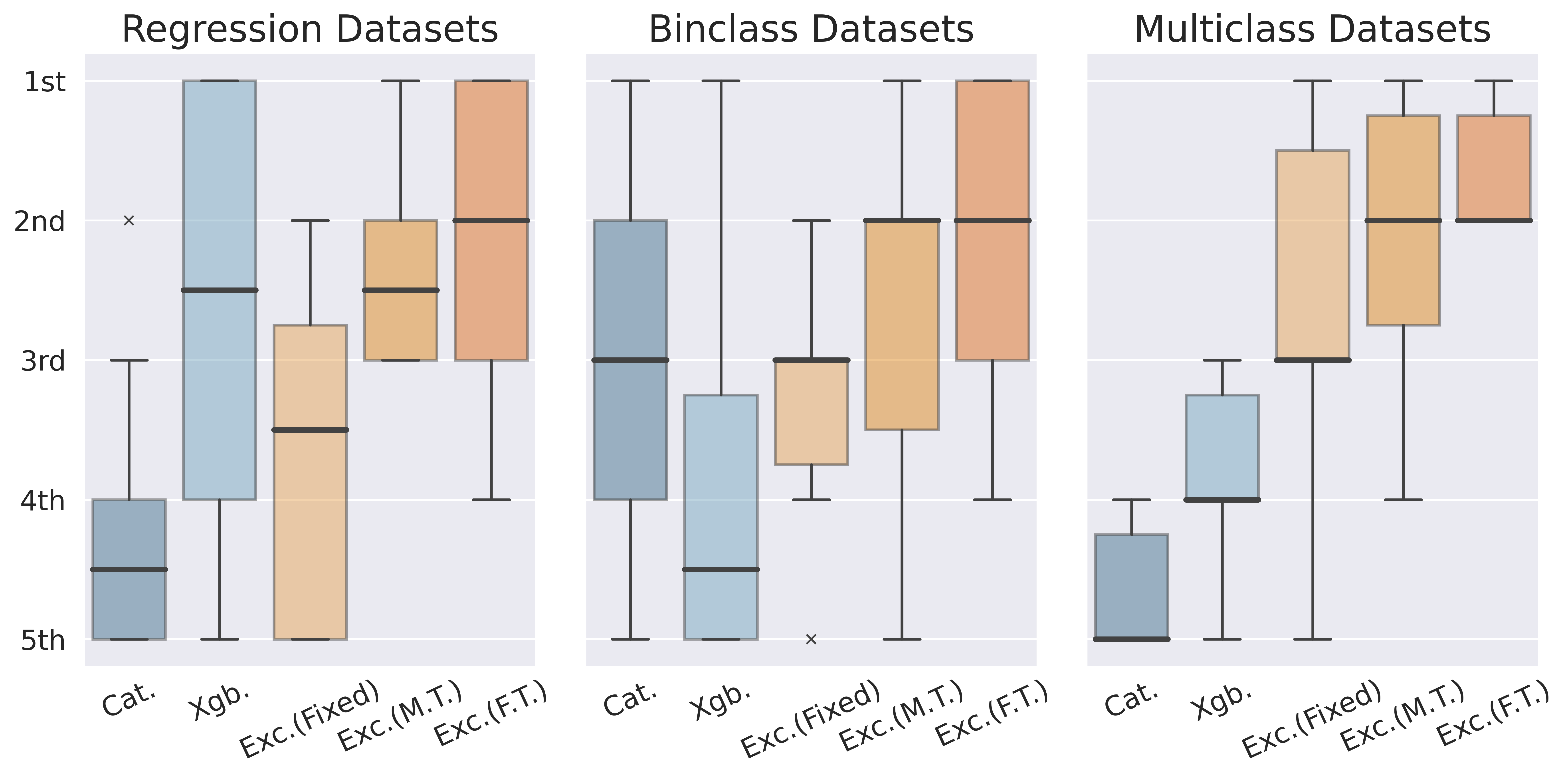
Figure 4: Model performances for different types of tasks. “Cat.”, “XGb.”, and “Exc.” denote “Catboost”, “XGboost”, and “ExcelFormer”, while “M.T.” and “F.T.” in the brackets indicate the “Mix Tuned” and “Fully Tuned” versions of ExcelFormer.

5.2 Performances

Performances of Untuned ExcelFormer. ExcelFormer-Feat-Mix (resp., ExcelFormer-Hidden-Mix) uses only our Feat-Mix (resp., Hidden-Mix) but not Hidden-Mix (resp., Feat-Mix). Their performances on all the 28 datasets are reported in Table 1. Both ExcelFormer-Feat-Mix and ExcelFormer-Hidden-Mix are trained with pre-specified hyper-parameters, without any hyper-parameter tuning. The average performance rank of ExcelFormer-Feat-Mix is 4.61, which is quite close to Catboost’s 4.36. The average rank of ExcelFormer-Hidden-Mix is 3.75, which falls between those of Catboost (4.36) and XGboost (3.43). In pairwise comparison, ExcelFormer-Feat-Mix beats the extensively tuned XGboost on 11 out of 28 datasets, while ExcelFormer-Hidden-Mix beats XGboost on 14 out of 28 datasets. In comparison with extensively tuned Catboost, ExcelFormer-Feat-Mix obtains better performances on 11 out of 28 datasets while ExcelFormer-Hidden-Mix obtains better performances on 15 out of 28 datasets. These results suggest that, by directly using ExcelFormer with the default hyper-parameters, one can easily obtain GBDT-level performances on tabular datasets. Due to the diversity of tabular datasets, a foolproof well-performed approach without tuning is very user-friendly and has a great potential for practical applications, as most users are not proficient in conducting hyper-parameter tuning.

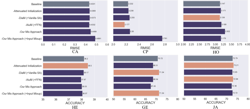
Figure 5: Ablation study on our proposed ingredients of ExcelFormer using six datasets. “–” denotes removal and “+” denotes inclusion. The bars colored in “ purple” indicate worse performances compared with the baseline, while the bars in “ orange” indicate better performances. Note that the lower “RMSE”, the better; the higher “ACCURACY”, the better.

Performances of Tuned ExcelFormer. By tuning the configurations of our Mixup schemes (i.e., the Mixup types and $\alpha$ of $\mathcal{B}eta$ distributions), the performance rank of ExcelFormer, 2.46, is much better than XGboost (3.43) and Catboost (4.36). In direct comparison to the extensively tuned XGboost, ExcelFormer with Mixup tuning (denoted by ExcelFormer (Mix Tuned)) is superior on 18 out of 28 datasets, and is superior on 24 out of 28 datasets comparing with the extensively tuned Catboost. These results suggest that a user can easily obtain considerably better performances than the extensively tuned XGboost and Catboost by tuning only two hyper-parameters of the Mixup configurations, without tuning the configurations of the model architecture.

Moreover, one can obtain further improved performances by tuning all the configurations (listed in Appendix B). In this way, ExcelFormer (denoted by ExcelFormer (Fully Tuned)) yields a better performance rank at 1.79, outperforming (or on par with) the extensively tuned XGboost and Catboost on 20 and 24 out of 28 datasets, respectively.

Observing the performance ranks over the 28 datasets, one can see that the fully tuned ExcelFormer performs better than its Mix tuned version, which is much better than ExcelFormer with fixed hyper-parameters. From the practical perspective, ExcelFormer with fixed hyper-parameters is sufficient to attain results on par with the extensively tuned XGboost/Catboost, and the tuned versions of ExcelFormer can yield remarkably better results.

5.3 Usage Suggestions

In practice, we would suggest that a user may use our ExcelFormer as follows: (1) first try ExcelFormer with fixed hyper-parameters, and it can meet the needs in most situations; (2) try the setting of “Mix Tuned” if the fixed ExcelFormer versions are not satisfactory; (3) finally, tune all the hyper-parameters of ExcelFormer if better performances are desired. Fig. 4 gives performance comparisons on different types of tasks, based on which we offer two further suggestions to users. (i) If extremely high effects are desired, it is wise to tune ExcelFormer following the “Mix Tuning” setting or “Fully Tuning” setting, for any type of tasks. (ii) For a multi-class classification task, ExcelFormer should be the first choice, since it commonly outperforms GBDTs, even without hyper-parameter tuning.

5.4 Ablation Study

We analyze the effects of our proposed ingredients empirically on 6 tabular datasets (we find that the conclusions on the other datasets are similar). We take the best-performing model of ExcelFormer-Feat-Mix and ExcelFormer-Hidden-Mix (without hyper-parameter tuning) as the baseline, and either remove or replace one ingredient each time for comparison. Fig. 5 reports the performances of the following ExcelFormer versions: (1) He’s initialization is used to replace our attenuated initialization approach for AiuM and DiaM, (2) a vanilla self-attention module (vanilla SA) is used to replace DiaM for heterogeneous feature interactions, (3) the linear feed-forward network (FFN) is used to replace AiuM for feature representation updates, (4) both Feat-Mix and Hidden-Mix are not used, and (5) the input Mixup (Zhang et al., 2018) ($\alpha=0.5$) is used to replace our proposed Mixup schemes. One can see that the performances often decrease when an ingredient is removed or replaced, suggesting that all of our ingredients are beneficial in general. But, it is also witnessed that the compared model versions perform worse than the baseline on 1 or 2 out of the 6 datasets, indicating that an ingredient may have negative impact on some datasets. In the model development, we retain all these designs since they show positive impacts on most of the datasets. Notably, it is difficult to optimize a design that is always effective since tabular data are of high diversity and our goal is to present a neural network that can accommodate as many tasks as possible.

Comparing the baseline with the versions with the input Mixup or with no Mixup, it is clear that our proposed Mixup schemes are more suitable to tabular data and are outperforming on 5 or 6 out of the 6 datasets, respectively. Comparing the no-Mixup version and the version with the input Mixup, the version with the input Mixup performs better on 4 out of 6 datasets; the no-Mixup version is better on the other 2 datasets. These results further indicate that using the input Mixup is not consistently effective across various tabular datasets, though it beats our proposed Mixup schemes on the GE dataset.

6 Conclusions

In this paper, we developed a new neural network model, ExcelFormer, for supervised tabular data tasks (e.g., classification and regression), and achieved performances beyond the level of GBDTs without bells and whistles. Our proposed ExcelFormer can achieve competitive performances compared to the extensively tuned XGboost and Catboost even without hyper-parameter tuning, while hyper-parameter tuning can improve ExcelFormer’s performances further. Such superiority is demonstrated by comprehensive experiments on 28 public tabular datasets, and is achieved by the cooperation of a simple but efficient model architecture and an accompanied training methodology. We expect that our ExcelFormer together with the training methodology will serve as an effective tool for supervised tabular data applications, and inspire future studies to develop better approaches for dealing with tabular data.

Appendix A Description of the Datasets Used

The details of the tabular datasets that we use are summarized in Table 2. We use the same train-valid-test split for all the approaches and the data pre-processing approaches as in (Gorishniy et al., 2021).

Table 2: The details of the datasets used. “# Num” and “# Cat” denote the numbers of numerical and categorical features, respectively. “# Sample” is for the size of a dataset.

Dataset	Abbr.	Task Type	Metric	# Features	# Num	# Cat	# Sample	Link
analcatdata_supreme	AN	regression	nRMSE	7	2	5	4,052	https://www.openml.org/d/44055
isolet	IS	multiclass	ACC	613	613	0	7,797	https://www.openml.org/d/44135
cpu_act	CP	regression	nRMSE	21	21	0	8,192	https://www.openml.org/d/44132
visualizing_soil	VI	regression	nRMSE	4	3	1	8,641	https://www.openml.org/d/44056
yprop_4_1	YP	regression	nRMSE	62	42	20	8,885	https://www.openml.org/d/44054
gesture	GE	multiclass	ACC	32	32	0	9,873	https://www.openml.org/d/4538
churn	CH	binclass	AUC	11	10	1	10,000	https://www.kaggle.com/shrutimechlearn/churn-modelling
sulfur	SU	regression	nRMSE	6	6	0	10,081	https://www.openml.org/d/44145
bank-marketing	BA	binclass	AUC	7	7	0	10,578	https://www.openml.org/d/44126
Brazilian_houses	BR	regression	nRMSE	8	8	0	10,692	https://www.openml.org/d/44141
eye	EY	multiclass	ACC	26	26	0	10,936	http://www.cis.hut.fi/eyechallenge2005
MagicTelescope	MA	binclass	AUC	10	10	0	13,376	https://www.openml.org/d/44125
Ailerons	AI	regression	nRMSE	33	33	0	13,750	https://www.openml.org/d/44137
pol	PO	regression	nRMSE	26	26	0	15,000	https://www.openml.org/d/722
binarized-pol	BP	binclass	AUC	48	48	0	15,000	https://www.openml.org/d/722
credit	CR	binclass	AUC	10	10	0	16,714	https://www.openml.org/d/44089
california	CA	regression	nRMSE	8	8	0	20,640	https://www.dcc.fc.up.pt/~ltorgo/Regression/cal_housing.html
house_sales	HS	regression	nRMSE	15	15	0	21,613	https://www.openml.org/d/44144
house	HO	regression	nRMSE	16	16	0	22,784	https://www.openml.org/d/574
diamonds	DI	regression	nRMSE	6	6	0	53,940	https://www.openml.org/d/44140
helena	HE	multiclass	ACC	27	27	0	65,196	https://www.openml.org/d/41169
jannis	JA	multiclass	ACC	54	54	0	83,733	https://www.openml.org/d/41168
higgs-small	HI	binclass	AUC	28	28	0	98,049	https://www.openml.org/d/23512
road-safety	RO	binclass	AUC	32	29	3	111,762	https://www.openml.org/d/44161
medicalcharges	ME	regression	nRMSE	3	3	0	163,065	https://www.openml.org/d/44146
SGEMM_GPU_kernel_performance	SG	regression	nRMSE	9	3	6	241,600	https://www.openml.org/d/44069
covtype	CO	multiclass	nRMSE	54	54	0	581,012	https://www.openml.org/d/1596
nyc-taxi-green-dec-2016	NY	regression	nRMSE	9	9	0	581,835	https://www.openml.org/d/44143

Appendix B Hyper-Parameter Tuning

For XGboost and Catboost, we follow the implementations in (Gorishniy et al., 2021), while increasing the number of estimators/iterations (i.e., decision trees) and the number of tuning iterations, so as to attain best-performing models. For our ExcelFormer, we apply the Optuna based tuning (Akiba et al., 2019). The hyper-parameter search spaces of ExcelFormer, XGboost, and Catboost are reported in Tables 3, 4, and 5, respectively. For ExcelFormer, we tune just 50 iterations on the configurations with our proposed Mixup schemes (Mix tuning), while for full tuning, we tune further 50 iterations using the acquired hyper-parameters from Mix tuning as initialization.

Table 3: The hyper-parameter tuning space for ExcelFormer. The items marked with “*” are used in the Mix tuning, while all the items are used in the full tuning.

Hyper-parameter	Distribution
# Layers $L$	UniformInt[2, 5]
Representation size $d$	{64, 128, 256}
# Heads	{4, 8, 16, 32}
Residual dropout rate	Uniform[0, 0.5]
Learning rate	LogUniform[$3\times 10^{-5}$, $10^{-3}$]
Weight decay	{0.0, LogUniform[$10^{-6}$, $10^{-3}$]}
(*) Mixup type	{Feat-Mix, Hidden-Mix }
(*) $\alpha$ of $\mathcal{B}eta$ distribution	Uniform[0.1, 3.0]

Table 4: The hyper-parameter tuning space for XGboost.

Hyper-parameter	Distribution
Booster	“gbtree”
N-estimators	Const(4096)
Early-stopping-rounds	Const(50)
Max depth	UniformInt[3, 10]
Min child weight	LogUniform[$10^{-8}$, $10^{5}$]
Subsample	Uniform[0.5, 1.0]
Learning rate	LogUniform[$10^{-5},1$]
Col sample by level	Uniform[0.5, 1]
Col sample by tree	Uniform[0.5, 1]
Gamma	{0, LogUniform[$10^{-8},10^{2}$]}
Lambda	{0, LogUniform[$10^{-8},10^{2}$]}
Alpha	{0, LogUniform[$10^{-8},10^{2}$]}
# Tuning iterations	500

Table 5: The hyper-parameter tuning space for Catboost.

Hyper-parameter	Distribution
Iterations (number of trees)	Const(4096)
Od pval	Const(0.001)
Early-stopping-rounds	Const(50)
Max depth	UniformInt[3, 10]
Learning rate	LogUniform[$10^{-5},1$]
Bagging temperature	Uniform[0, 1]
L2 leaf reg	LogUniform[1, 10]
Leaf estimation iterations	UniformInt[1, 10]
# Tuning iterations	500

References

- Akiba et al. (2019) Akiba, T., Sano, S., Yanase, T., Ohta, T., and Koyama, M. Optuna: A next-generation hyperparameter optimization framework. In The ACM SIGKDD International Conference on Knowledge Discovery & Data Mining, 2019.
- Arik & Pfister (2021) Arik, S. Ö. and Pfister, T. TabNet: Attentive interpretable tabular learning. In The AAAI Conference on Artificial Intelligence, 2021.
- Ba et al. (2016) Ba, J. L., Kiros, J. R., and Hinton, G. E. Layer normalization. arXiv preprint arXiv:1607.06450, 2016.
- Bachlechner et al. (2021) Bachlechner, T., Majumder, B. P., Mao, H., Cottrell, G., and McAuley, J. Rezero is all you need: Fast convergence at large depth. In Uncertainty in Artificial Intelligence, 2021.
- Borisov et al. (2021) Borisov, V., Leemann, T., Seßler, K., Haug, J., Pawelczyk, M., and Kasneci, G. Deep neural networks and tabular data: A survey. arXiv preprint arXiv:2110.01889, 2021.
- Chen et al. (2020) Chen, J., Yu, H., Feng, R., Chen, D. Z., and Wu, J. Flow-Mixup: Classifying multi-labeled medical images with corrupted labels. In International Conference on Bioinformatics and Biomedicine, 2020.
- Chen et al. (2022) Chen, J., Liao, K., Wan, Y., Chen, D. Z., and Wu, J. DANets: Deep abstract networks for tabular data classification and regression. In The AAAI Conference on Artificial Intelligence, 2022.
- Chen et al. (2023) Chen, J., Liao, K., Fang, Y., Chen, D. Z., and Wu, J. TabCaps: A capsule neural network for tabular data classification with BoW routing. In International Conference on Learning Representations, 2023.
- Chen & Guestrin (2016) Chen, T. and Guestrin, C. XGBoost: A scalable tree boosting system. In ACM SIGKDD International Conference on Knowledge Discovery and Data Mining, 2016.
- Cheng et al. (2016) Cheng, H.-T., Koc, L., Harmsen, J., et al. Wide & deep learning for recommender systems. In Workshop on Deep Learning for Recommender Systems, 2016.
- Darabi et al. (2021) Darabi, S., Fazeli, S., Pazoki, A., Sankararaman, S., and Sarrafzadeh, M. Contrastive Mixup: Self-and semi-supervised learning for tabular domain. arXiv preprint arXiv:2108.12296, 2021.
- Dong et al. (2018) Dong, L., Xu, S., and Xu, B. Speech-Transformer: A no-recurrence sequence-to-sequence model for speech recognition. In International Conference on Acoustics, Speech and Signal Processing, 2018.
- Duan et al. (2020) Duan, T., Anand, A., Ding, D. Y., Thai, K. K., Basu, S., Ng, A., and Schuler, A. NGBoost: Natural gradient boosting for probabilistic prediction. In International Conference on Machine Learning, 2020.
- Glorot & Bengio (2010) Glorot, X. and Bengio, Y. Understanding the difficulty of training deep feedforward neural networks. In International Conference on Artificial Intelligence and Statistics, 2010.
- Gorishniy et al. (2021) Gorishniy, Y., Rubachev, I., Khrulkov, V., and Babenko, A. Revisiting deep learning models for tabular data. In Advances in Neural Information Processing Systems, 2021.
- Gorishniy et al. (2022) Gorishniy, Y., Rubachev, I., and Babenko, A. On embeddings for numerical features in tabular deep learning. In Advances in Neural Information Processing Systems, 2022.
- Grinsztajn et al. (2022) Grinsztajn, L., Oyallon, E., and Varoquaux, G. Why do tree-based models still outperform deep learning on typical tabular data? In Advances in Neural Information Processing Systems, 2022.
- Guo et al. (2017) Guo, H., Tang, R., Ye, Y., Li, Z., and He, X. DeepFM: A factorization-machine based neural network for CTR prediction. In International Joint Conference on Artificial Intelligence, 2017.
- Guo et al. (2021) Guo, H., Chen, B., Tang, R., Zhang, W., Li, Z., and He, X. An embedding learning framework for numerical features in CTR prediction. In ACM SIGKDD Conference on Knowledge Discovery and Data Mining, 2021.
- He et al. (2015) He, K., Zhang, X., Ren, S., and Sun, J. Delving deep into rectifiers: Surpassing human-level performance on ImageNet classification. In International Conference on Computer Vision, 2015.
- Hochreiter & Schmidhuber (1997) Hochreiter, S. and Schmidhuber, J. Long short-term memory. Neural Computation, 1997.
- Kadra et al. (2021) Kadra, A., Lindauer, M., Hutter, F., and Grabocka, J. Well tuned simple nets excel on tabular datasets. Advances in Neural Information Processing Systems, 2021.
- Katzir et al. (2020) Katzir, L., Elidan, G., and El-Yaniv, R. Net-DNF: Effective deep modeling of tabular data. In International Conference on Learning Representations, 2020.
- Khan et al. (2022) Khan, S., Naseer, M., Hayat, M., Zamir, S. W., Khan, F. S., and Shah, M. Transformers in vision: A survey. ACM Computing Surveys, 2022.
- Kim et al. (2020) Kim, J.-H., Choo, W., and Song, H. O. Puzzle Mix: Exploiting saliency and local statistics for optimal mixup. In International Conference on Machine Learning, 2020.
- Loshchilov & Hutter (2018) Loshchilov, I. and Hutter, F. Decoupled weight decay regularization. In International Conference on Learning Representations, 2018.
- Ng (2004) Ng, A. Y. Feature selection, L1 vs. L2 regularization, and rotational invariance. In International Conference on Machine Learning, 2004.
- Popov et al. (2019) Popov, S., Morozov, S., and Babenko, A. Neural oblivious decision ensembles for deep learning on tabular data. In International Conference on Learning Representations, 2019.
- Prokhorenkova et al. (2018) Prokhorenkova, L., Gusev, G., Vorobev, A., Dorogush, A. V., and Gulin, A. CatBoost: Unbiased boosting with categorical features. Advances in Neural Information Processing Systems, 2018.
- Qin et al. (2020) Qin, J., Fang, J., Zhang, Q., Liu, W., Wang, X., and Wang, X. ResizeMix: Mixing data with preserved object information and true labels. arXiv preprint arXiv:2012.11101, 2020.
- Radford et al. (2018) Radford, A., Narasimhan, K., et al. Improving language understanding by generative pre-training. https://s3-us-west-2.amazonaws.com/openai-assets/research-covers/language-unsupervised/language_understanding_paper.pdf, 2018.
- Rahaman et al. (2019) Rahaman, N., Baratin, A., Arpit, D., Draxler, F., Lin, M., Hamprecht, F., Bengio, Y., and Courville, A. On the spectral bias of neural networks. In International Conference on Machine Learning, 2019.
- Saxe et al. (2014) Saxe, A. M., McClelland, J. L., and Ganguli, S. Exact solutions to the nonlinear dynamics of learning in deep linear neural networks. In International Conference on Learning Representations, 2014.
- Somepalli et al. (2021) Somepalli, G., Goldblum, M., Schwarzschild, A., Bruss, C. B., and Goldstein, T. SAINT: Improved neural networks for tabular data via row attention and contrastive pre-training. arXiv preprint arXiv:2106.01342, 2021.
- Srivastava et al. (2015) Srivastava, R. K., Greff, K., and Schmidhuber, J. Highway networks. In International Conference on Machine Learning Workshop, 2015.
- Tajbakhsh et al. (2020) Tajbakhsh, N., Jeyaseelan, L., Li, Q., Chiang, J. N., Wu, Z., and Ding, X. Embracing imperfect datasets: A review of deep learning solutions for medical image segmentation. Medical Image Analysis, 2020.
- Tancik et al. (2020) Tancik, M., Srinivasan, P., Mildenhall, B., Fridovich-Keil, S., Raghavan, N., Singhal, U., Ramamoorthi, R., Barron, J., and Ng, R. Fourier features let networks learn high frequency functions in low dimensional domains. Advances in Neural Information Processing Systems, 2020.
- Touvron et al. (2021a) Touvron, H., Cord, M., Douze, M., Massa, F., Sablayrolles, A., and Jégou, H. Training data-efficient image Transformers & distillation through attention. In International Conference on Machine Learning, 2021a.
- Touvron et al. (2021b) Touvron, H., Cord, M., Sablayrolles, A., Synnaeve, G., and Jégou, H. Going deeper with image Transformers. In IEEE/CVF International Conference on Computer Vision, 2021b.
- Uddin et al. (2020) Uddin, A. S., Monira, M. S., Shin, W., Chung, T., and Bae, S.-H. SaliencyMix: A saliency guided data augmentation strategy for better regularization. In International Conference on Learning Representations, 2020.
- Vaswani et al. (2017) Vaswani, A., Shazeer, N., Parmar, N., Uszkoreit, J., Jones, L., Gomez, A. N., Kaiser, Ł., and Polosukhin, I. Attention is all you need. Advances in Neural Information Processing Systems, 2017.
- Verma et al. (2019) Verma, V., Lamb, A., Beckham, C., Najafi, A., Mitliagkas, I., Lopez-Paz, D., and Bengio, Y. Manifold Mixup: Better representations by interpolating hidden states. In International Conference on Machine Learning, 2019.
- Walawalkar et al. (2020) Walawalkar, D., Shen, Z., Liu, Z., and Savvides, M. Attentive Cutmix: An enhanced data augmentation approach for deep learning based image classification. In International Conference on Acoustics, Speech and Signal Processing, 2020.
- Wang & Sun (2022) Wang, Z. and Sun, J. TransTab: Learning transferable tabular Transformers across tables. In Advances in Neural Information Processing Systems, 2022.
- Wang et al. (2020) Wang, Z., Zhang, W., Ning, L., and Wang, J. Transparent classification with multilayer logical perceptrons and random binarization. In The AAAI Conference on Artificial Intelligence, 2020.
- Wang et al. (2021) Wang, Z., Zhang, W., Liu, N., and Wang, J. Scalable rule-based representation learning for interpretable classification. Advances in Neural Information Processing Systems, 2021.
- Yan et al. (2023) Yan, J., Chen, J., Wu, Y., Chen, D. Z., and Wu, J. T2G-former: Organizing tabular features into relation graphs promotes heterogeneous feature interaction. The AAAI Conference on Artificial Intelligence, 2023.
- Yoon et al. (2020) Yoon, J., Zhang, Y., Jordon, J., and van der Schaar, M. VIME: Extending the success of self-and semi-supervised learning to tabular domain. Advances in Neural Information Processing Systems, 2020.
- Yun et al. (2019) Yun, S., Han, D., Oh, S. J., Chun, S., Choe, J., and Yoo, Y. CutMix: Regularization strategy to train strong classifiers with localizable features. In International Conference on Computer Vision, 2019.
- Zhang et al. (2021) Zhang, C., Bengio, S., Hardt, M., Recht, B., and Vinyals, O. Understanding deep learning requires rethinking generalization. Communications of the ACM, 2021.
- Zhang et al. (2018) Zhang, H., Cisse, M., Dauphin, Y. N., and Lopez-Paz, D. Mixup: Beyond empirical risk minimization. In International Conference On Learning Representations, 2018.