DoD stabilization for higher-order advection in two dimensions
Abstract
When solving time-dependent hyperbolic conservation laws on cut cell meshes one has to overcome the small cell problem: standard explicit time stepping is not stable on small cut cells if the time step is chosen with respect to larger background cells. The domain of dependence (DoD) stabilization is designed to solve this problem in a discontinuous Galerkin framework. It adds a penalty term to the space discretization that restores proper domains of dependency. In this contribution we introduce the DoD stabilization for solving the advection equation in 2d with higher order. We show an stability result for the stabilized semi-discrete scheme for arbitrary polynomial degrees and provide numerical results for convergence tests indicating orders of in the norm and between and in the norm.
1 Introduction
Modern simulations often require to mesh complex geometries. One approach that is particularly suited for this purpose are embedded boundary meshes. One simply cuts the geometry out of a structured background mesh, resulting in cut cells along the boundary of the embedded object. Cut cells have different shapes and can become arbitrarily small. In the context of solving time-dependent hyperbolic conservation laws this causes the small cell problem: for standard explicit time stepping, the scheme is not stable on small cut cells when the time step is chosen with respect to the larger background cells.
Existing solution approaches in a finite volume regime are typically bound to at most second order, see for example the flux redistribution method Chern_Colella ; Colella2006 , the -box method Berger_Helzel_Leveque_2005 ; Berger_Helzel_2012 , the mixed explicit-implicit scheme May_Berger_explimpl , the dimensionally split approach Klein_cutcell ; Klein_cutcell_3d , or the state redistribution (SRD) method Berger_Giuliani_2021 . An exception is the extension of the active flux method to cut cell meshes FVCA_Helzel_Kerkmann , which aims for third order.
For discontinuous Galerkin (DG) schemes it is significantly easier to achieve higher order. The development of DG schemes that overcome the small cell problem has only started very recently. Some work relies on cell merging, e.g. Kronbichler2020 , other work on algorithmic solution approaches such as the usage of a ghost penalty term as done by Fu and Kreiss Kreiss_Fu or the extension of the SRD method to a DG setting by Giuliani Giuliani_DG .
Another approach, proposed previously by the authors, is the Domain-of-Dependence (DoD) stabilization. In this approach, a penalty term is added on small cut cells that restores the proper domains of dependence in the neighborhood of small cut cells and therefore makes standard explicit time stepping stable again. In DoD_SIAM_2020 we first introduced the DoD stabilization for linear advection in 1d and 2d for linear polynomials only. In DoD_AMC_2021 , we extend the stabilization in 1d to non-linear systems and higher order. For the extension to higher order in 1d we found that it is necessary to add an extra term in the stabilization, which adjusts the mass distribution within inflow neighbors of small cut cells. With this term it is possible to show an stability result for the semi-discrete setting (keeping the time continuous) in 1d DoD_AMC_2021 .
In this contribution, we partially extend the 1d results from DoD_AMC_2021 to 2d by solving linear advection with higher order polynomials. For the case of a planar ramp geometry we show an stability result for the semi-discrete setting. We will also provide corresponding numerical results. These results show the expected convergence orders of for polynomial degree in the norm. In the norm, we observe a slight decay, resulting in convergence orders between and .
2 Problem setup
Within the scope of this work, we will focus on the 2d linear advection equation
| (1) | ||||||
| (2) | ||||||
| (3) |
We denote by an open, connected domain in and by its boundary. The inflow boundary is defined as with being the outer unit normal vector on . Analogously, we define . Moreover, is the velocity field and the standard scalar product in .
For simplicity and brevity of presentation, we will focus in this presentation on the case of a ramp geometry with a constant velocity field , which is parallel to the ramp. The geometry setup and mesh creation is sketched in figure 1. We refer to the internal and external faces of our mesh as
| (4) | ||||
| (5) |
with denoting the length of an edge . We then further split in and : contains all Cartesian boundary faces and contains the boundary faces along the ramp that were created by cutting out the ramp geometry.
On the partition , we define the discrete function space by
| (6) |
where denotes the polynomial space of degree .
On a face between two adjacent cells and , i.e., , we define the scalar-valued average as
and the jump to be vector-valued as
| (7) |
with denoting the outer unit normal vector of cell , . With these prerequisites we can now define the scheme that we use to solve (1).
We use a method of lines approach: we first discretize in space and then in time. The unstabilized semi-discrete scheme is given by: Find such that
| (8) |
with
| (9) | |||
| (10) |
Here, denotes the standard scalar product in and is a unit normal on a face (of arbitrary but fixed orientation). We define the negative and positive parts of as and Note that that the standard upwind flux is used in the definition of .
The proposed stabilization modifies the space discretization, whereas in time we are free to use a time stepping scheme of our choice. We will use standard explicit strong stability preserving (SSP) Runge Kutta (RK) schemes GottliebShuTadmor .
3 Stabilization terms
The stabilization is designed as an additional term that is added to the semi-discrete formulation in (8). The DoD stabilized semi-discrete scheme is then given by: Find such that
| (11) |
The stabilization term is given by
We define and in detail below. The set denotes the set of small cut cells that need stabilization. For a planar cut in 2d, there are 3-sided, 4-sided, and 5-sided cut cells. In DoD_SIAM_2020 , we have shown (see Lemma 3.5), that for the considered setup, it is sufficient to stabilize triangular cut cells only. For a triangular cut cell in our setup, each edge has a different boundary condition, see figure 2:
-
•
On the boundary edge we have a no-flow boundary condition as the flow is parallel to the ramp.
-
•
Out of the two remaining edges, one edge is the inflow edge , which is characterized by .
-
•
The remaining edge is the outflow edge , which is characterized by .
Thus we can uniquely define an inflow neighbor and an outflow neighbor for a triangular cut cell .
If the time step is chosen according to the size of the larger background cells and does not respect the size of small cut cells, then, physically, mass passes within one time step from the inflow cell through the small cut cell into the outflow cell . The idea behind the DoD stabilization is to make this possible by directly passing part of the mass that enters from into the outflow neighbor . This way we restore the domain of dependence of the outflow neighbor and make sure that the small cut cell only keeps as much mass as it can hold. For the latter one we define the concept of capacity below.
In order to create this flux of information between the inflow neighbor and the outflow neighbor of , we introduce an extension operator: The operator extends a function from a cell to the whole domain . This simply corresponds to evaluating a polynomial outside its original support. In particular, we will evaluate the polynomial solution defined on cell to . We will refer to this both as , , as well as simply as to ease notation.
With these prerequisites we can now define and . Generally, the terms of the DoD stabilization target two different goals:
-
•
aims for redistributing the mass among the small cut cells and their neighbors appropriately. It therefore consists of cell interface terms.
-
•
aims for redistributing the mass within the small cut cells and their neighbors appropriately. It therefore consists of volume terms.
The term is given by
| (12) |
with the stabilization parameter defined below. Note that we only redistribute mass across outflow edges of small cut cells and that we use the extended solution of the inflow neighbor to determine the size of the correction. The term is given by
| (13) |
This term is designed to adjust the mass distribution primarily within the small cut cell and secondarily within its neighbor. Note that we apply the extension operator to both the discrete solution and the test function from inflow neighbor . In DoD_SIAM_2020 , where we only considered piecewise linear polynomials, we proposed a different formulation of , which did not contain the term . In 1d DoD_AMC_2021 , we found that when going to higher order one can run into instabilities without this extra term. In addition, with this augmented definition of we are able to show an stability result for the semi-discrete scheme, which we will present below.
Both stabilization terms are scaled with the stabilization parameter . We set with the capacity and being the polynomial degree of the discrete function space. We define the capacity of a cut cell , see DoD_SIAM_2020 , as
| (14) |
For , the capacity estimates the fraction of the inflow that is allowed to flow into the cut cell and stay there without producing overshoot. Note that by definition .
3.1 stability for semi-discrete scheme
In the following we will show an stability result for the stabilized semi-discrete scheme for an arbitrary polynomial degree . Generally, the stability result for the considered ramp setup is influenced by the inflow and outflow across and during the time . Note that only Cartesian faces are contained in as we have a no-flow boundary condition for faces along the ramp. Our goal here is to show that stability still holds true for the stabilized scheme with cut cells being present, and not to analyze the influence of the inflow and outflow on the stability. We will therefore for simplicity assume that the solution has compact support inside during the considered time interval and does not intersect the Cartesian boundary, i.e. , which implies that we have a homogeneous right hand side during the whole time frame and in particular that there is no in- or outflow.
Theorem 3.1
Proof
Setting in (11) and ignoring boundary contributions with respect to , we get
Integration of the first term in time yields
and it remains to show that for any fixed
We will first discuss and then . (We will drop the explicit time dependency in the following for brevity.)
By definition of and ignoring outflow across , there holds
For the integral term we rewrite
Let us first consider a standard Cartesian cell with edges as shown in figure 3. Then, for , there holds
For the edge terms in , let us consider the internal edge , connecting and . Then, (using from now on the notation to indicate that we evaluate the discrete solution from cell , potentially outside of its original support)
Combining this with the corresponding contributions for edge from the volume terms from cells and , we get
Let us now add the cut cells. For the small triangular cut cell with the notation from figure 2, we get with
Therefore, taking the boundary term in into account as well as the contribution from the volume term of cell , we get for the edge
We obtain a similar term for edge , involving solutions from cells and . Therefore, ignoring boundary contributions across due to the assumption of compact support, there holds
| (15) |
Therefore, without the stabilization term , there holds stability.
Let us now add the stabilization term
We only stabilize small triangular cells of type . There holds
We now consider given by
With , there holds
As , the negative term over the edge can be compensated with the edge term from in (15). For the edge , we collect all terms from and to get
The right term in the last line involves the standard jump over edge and (same as for edge ) can be compensated with its positive counterpart in the sum in (15). The first term in the last line consists of a new extended jump involving the difference of the solution of cell and the solution of cell , both evaluated on the outflow edge . This concludes the proof.
4 Numerical results
In this section, we present numerical results for the linear advection equation in 2d using higher order polynomials for the ramp setup introduced above for different angles , see figure 1. We choose and start the ramp at . For the definition of the initial data, we use a rotated and shifted coordinate system that we derive from the standard Cartesian coordinate system by
| (16) |
This newly described coordinate system is defined in such a way that the -direction is parallel and the -direction is orthogonal to the ramp. In this coordinate system, the velocity field and the smooth initial data are given by
We derive the inflow conditions on from the exact solution. We compute the discrete solution at time using polynomials of degrees . In time we use an SSP RK scheme of the same order as the space discretization. We compute the time step by
| (17) |
Here, with being the number of cells in - and -direction on .
The implementation is based on the DUNE dune08:1 ; dune08:2 framework, the cut-cell DG extension dune-udg package duneudg ; Bastian_Engwer and its integration with dune-pdelab. The geometry is represented as a discrete level set function, using vertex values. Based on this representation the cut cells and their corresponding quadrature rules are constructed via the TPMC library tpmc .
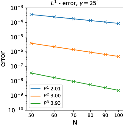
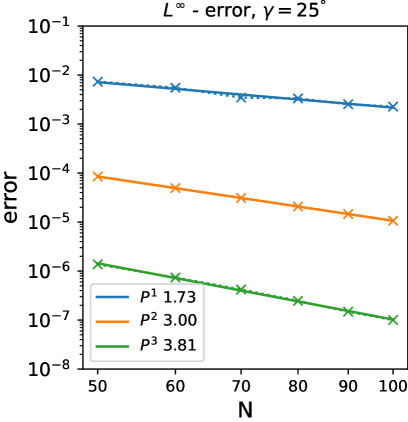
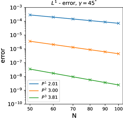
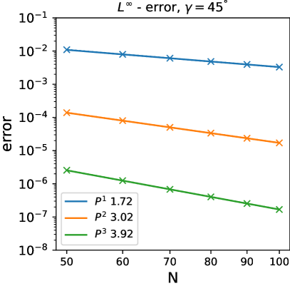
In figure 4, we show convergence results for ramp angles of and in the and norm. In the norm we observe convergence orders that are (roughly) for polynomials of degree for both angles. In the norm, the results are between and with less decay for even polynomial degrees. This is overall consistent with the findings of Giuliani Giuliani_DG who reports for the annulus test for the error orders between and for polynomials of degrees .
5 Conclusion
In this contribution, we introduce the formulation of the DoD stabilization for the linear advection equation for higher order polynomials. Compared to DoD_SIAM_2020 , where we only considered linear polynomials, we have augmented the penalty term to also involve the extended test function of the inflow neighbor of a small cut cell. For this new formulation, we show an stability result for the semi-discrete stabilized scheme for the ramp geometry. We also provide numerical results for a smooth test function, showing convergence rates between and for polynomial degree . In the future, we plan to extend the stabilization to non-linear problems in 2d.
References
- (1) Bastian, P., Blatt, M., Dedner, A., Engwer, C., Klöfkorn, R., Kornhuber, R., Ohlberger, M., Sander, O.: A generic grid interface for parallel and adaptive scientific computing. Part II: Implementation and tests in DUNE. Computing 82(2–3), 121–138 (2008). DOI 10.1007/s00607-008-0004-9
- (2) Bastian, P., Blatt, M., Dedner, A., Engwer, C., Klöfkorn, R., Ohlberger, M., Sander, O.: A generic grid interface for parallel and adaptive scientific computing. Part I: Abstract framework. Computing 82(2–3), 103–119 (2008). DOI 10.1007/s00607-008-0003-x
- (3) Bastian, P., Engwer, C.: An unfitted finite element method using discontinuous Galerkin. Internat. J. Numer. Methods Engrg. 79, 1557–1576 (2009)
- (4) Berger, M., Giuliani, A.: A state redistribution algorithm for finite volume schemes on cut cell meshes. J. Comput. Phys. 428 (2021). DOI 10.1016/j.jcp.2020.109820
- (5) Berger, M., Helzel, C.: A simplified h-box method for embedded boundary grids. SIAM J. Sci. Comput. 34(2), A861–A888 (2012)
- (6) Chern, I.L., Colella, P.: A conservative front tracking method for hyperbolic conservation laws. Tech. rep., Lawrence Livermore National Laboratory, Livermore, CA (1987). Preprint UCRL-97200
- (7) Colella, P., Graves, D.T., Keen, B.J., Modiano, D.: A Cartesian grid embedded boundary method for hyperbolic conservation laws. J. Comput. Phys. 211(1), 347–366 (2006)
- (8) Engwer, C., Heimann, F.: Dune-udg: a cut-cell framework for unfitted discontinuous Galerkin methods. In: Advances in DUNE, pp. 89–100. Springer (2012)
- (9) Engwer, C., May, S., Nüßing, A., Streitbürger, F.: A stabilized DG cut cell method for discretizing the linear transport equation. SIAM J. Sci. Comput. 42(6), A3677–A3703 (2020)
- (10) Engwer, C., Nüßing, A.: Geometric reconstruction of implicitly defined surfaces and domains with topological guarantees. ACM Trans. Math. Software (TOMS) 44(2), 14 (2017)
- (11) Fu, P., Kreiss, G.: High order cut discontinuous Galerkin methods for hyperbolic conservation laws in one space dimension. SIAM J. Sci. Comput. 43(4), A2404–A2424 (2021)
- (12) Giuliani, A.: A two-dimensional stabilized discontinuous Galerkin method on curvilinear embedded boundary grids (2021). ArXiv:2102.01857
- (13) Gokhale, N., Nikiforakis, N., Klein, R.: A dimensionally split Cartesian cut cell method for hyperbolic conservation laws. J. Comput. Phys. 364, 186–208 (2018)
- (14) Gottlieb, S., Shu, C.W., Tadmor, E.: Strong stability-preserving high-order time discretization methods. SIAM Rev. 43(1), 89–112 (2001)
- (15) Helzel, C., Berger, M., LeVeque, R.: A high-resolution rotated grid method for conservation laws with embedded geometries. SIAM J. Sci. Comput. 26(3), 785–809 (2005)
- (16) Helzel, C., Kerkmann, D.: An active flux method for cut cell grids. In: R. Klöfkorn, E. Keilegavlen, A. Radu, J. Fuhrmann (eds.) Finite Volumes for Complex Applications IX - Methods, Theoretical Aspects, Examples, pp. 507–515. Springer International Publishing (2020)
- (17) Klein, R., Bates, K.R., Nikiforakis, N.: Well-balanced compressible cut-cell simulation of atmospheric flow. Philos. Trans. Roy. Soc. A 367, 4559–4575 (2009)
- (18) May, S., Berger, M.: An explicit implicit scheme for cut cells in embedded boundary meshes. J. Sci. Comput. 71, 919–943 (2017)
- (19) May, S., Streitbürger, F.: DoD stabilization for non-linear hyperbolic conservation laws on cut cell meshes in one dimension. Appl. Math. Comput. 419 (2022)
- (20) Schoeder, S., Sticko, S., Kreiss, G., Kronbichler, M.: High‐order cut discontinuous Galerkin methods with local time stepping for acoustics. Internat. J. Numer. Methods Engrg. 121(13), 2979–3003 (2020)