Choked accretion onto Kerr-Sen black holes in Einstein-Maxwell-Dilation-Axion gravity

Abstract

We study the choked accretion process of an ultrarelativistic fluid onto axisymmetric Kerr-Sen black holes in Einstein-Maxwell-Dilation-Axion theory. We calculate the solution describing the velocity potential $\Phi$ of a stationary, irrotational fluid, which satisfies the stiff equation of state and draw the streamlined diagram of the quadrupolar flow solution. We investigate how parameters affect the solution’s coefficient and stagnation point. The injection rate, ejection rate, and critical angle are discussed in detail at the end of the article. If the inner and outer event horizons of the black hole are satisfied, then we can find that the ratio of the ejection rate to the setting rate increases with an increase in the dilation parameter.

I Introduction

The most probable scenario for explaining the high energy output from active galactic nuclei and quasars is matter accretion onto a black hole, which is a significant phenomenon for astrophysicists. The theory of black hole accretion also provides the most credible exposition for the high energy outflow from X-ray Binaries and Gamma Ray Bursts Abramowicz:2011xu . The investigations of the accretion processes onto celestial objects were initiated by Hoyle and Lyttleton hoyle_lyttleton_1939 ; hoyle_lyttleton_1940_1 ; hoyle_lyttleton_1940_2 ; 1941MNRAS.101..227H , and later studies were carried out by Bondi and Hoyle for a pressure-less gas falling onto a moving star Bondi:1944jm . Subsequently, the theory of stationary, spherically symmetric, and transonic hydrodynamic accretion of adiabatic fluid onto a gravitating astrophysical body at rest was formulated in a seminal paper by Bondi Bondi:1952ni , such a model was perfectly generalized by Michel to the Schwarzschild black hole of general relativity Michel1972 . Further research was constructed for distinct black hole backgrounds, various accreted constituents, and several alternative models see for example Malec:1999dd ; Babichev:2004yx ; Jiao:2016iwp ; Ganguly:2014cqa ; Yang:2015sfa ; Font:1998sc ; Yang:2019qru . Accretion onto Charged or rotating black holes were explored in Parev:1995me ; Font:1998sc ; Medvedev:2002wn ; Fragile:2004gp ; Bhadra:2011me ; JimenezMadrid:2005rk ; Feng:2022bst which used the same processing approach. In order to be as close as possible to real astrophysical processes, a precise completely relativistic solution describing stationary accretion of matter onto a moving Schwarzschild or Kerr black hole with an adiabatic equation of state was derived in Petrich:1988zz , which was generalized to Reissner-Nordström and charged dilaton black hole Jiao:2016uiv ; Yang:2021opo . Recently, the accretion of Vlasov gas onto a moving Schwarzschild black hole was proposed in Mach:2021zqe ; Mach:2020wtm ; Cai:2022fdu , it is discussed analytically by using the Hamiltonian form without considering the reaction of matter. Besides these analytical works, more realistic situations were considered in background of astronomical environments DiMatteo:2002hif ; Silich:2008xz ; Gil-Merino:2011yhj ; Kuo:2014pqa ; He:2022lrc .

On the other hand, the astrophysical jet is an astronomical phenomenon in which plasma matter is emitted as an extended beam along the rotation axis. Blandford, Payne (BP), and Blandford, Znajek (BZ) proposed the jet mechanism most widely accepted by previous works 10.1093/mnras/199.4.883 ; 10.1093/mnras/179.3.433 . BP mechanism utilizes magnetic centrifugation to extract energy and angular momentum from a black hole accretion disc, whereas the BZ mechanism involves rotational energy from a Kerr black hole. These methods were commonly used in magneto-hydrodynamics and astrophysics exploration Semenov:2004ib ; McKinney:2006tf ; Qian:2018qpg ; Liska:2018ayk . Afterward, a new hydrodynamic accretion mechanism was proposed that explains the effect of the steady-state axisymmetric partial fluid flowing from the equatorial plane being ejected along poles by the cytaster’s gravitational influence https://doi.org/10.48550/arxiv.1103.0250 . This process were also generalized to the choked accretion scenario of Schwarzschild and Kerr black holes in general relativity Tejeda:2019fwr ; Aguayo-Ortiz:2020qro .

In this paper, we will discuss the choked accretion process of ultrarelativistic perfect fluid onto rotating Kerr-Sen black holes in Einstein-Maxwell-Dilation-Axion (EMDA) theory, where an irrotational, steady-state hydrodynamic flow with finite boundary conditions at the horizon is considered. In particular, we will present a streamlined diagram of choked accretion based on the stiff equation of the state of perfect fluid and will investigate how the parameters affect the position of stagnation point and the relative density disparity.

The article is organized as follows: In Section II, the EMDA model and the Kerr-Sen black hole will be briefly reviewed. In Section III, based on the assumption of irrotational fluids, we will derive an analytical solution for the velocity potential $\Phi$ in Boyer-Lindquist coordinate system. In Section IV, The quadrupolar flow solution will be used to analyze the variation of the coefficients with parameters and will be displayed the streamline and temperature diagrams in the ZAMO frame. Finally, we will present in the mechanism of choked accretion the density ratio, the injection rate, the ejection rate, and as well as the value range of the reference point. For convenience, we will use geometrical units $c=G=1$ and signature convention $(-,+,+,+)$ for spacetime metric throughout the article.

II Kerr-Sen black hole in Einstein-Maxwell-Dilaton-Axion gravity

The Einstein-Maxwell-Dilaton-Axion gravity (EMDA) model is derived from the low energy limit behavior of heterotic string theory, it is composed of dilaton field $\chi$, gauge vector field $A_{\mu}$, metric $g_{\mu\nu}$, and pseudo-scalar axion field $\xi$ Sen:1992ua ; Rogatko:2002qe ; Campbell:1992hc . The action of the EMDA model could be formed by the coupling of supergravity and super-Yang Mills theory, it can be described by the following form,

$$S=\frac{1}{16\pi}\int\sqrt{-g}d^{4}x\left[\tilde{R}-2\partial_{\mu}\chi\partial^{\mu}\chi-\frac{1}{2}\mathrm{e}^{4\chi}\partial_{\mu}\xi\partial^{\mu}\xi+\mathrm{e}^{-2\chi}F_{\mu\nu}F^{\mu\nu}+\xi F_{\mu\nu}\widetilde{F}^{\mu\nu}\right],$$ (1)

where $\tilde{R}$ is the Ricci scalar and $F_{\mu\nu}$ is the second-order antisymmetric Maxwell field strength tensor with $F_{\mu\nu}=\nabla_{\mu}A_{\nu}-\nabla_{\nu}A_{\mu}$, $\widetilde{F}^{\mu\nu}$ is the dual tensor of the field strength. The variation of the aforementioned four fields yields the following motion equations:

$$\left\{\begin{split}&\Box\chi-\frac{1}{2}\mathrm{e}^{4\chi}\nabla_{\mu}\xi\nabla^{\mu}\xi+\frac{1}{2}\mathrm{e}^{-2\chi}F_{\mu\nu}F^{\mu\nu}=0\\ &\Box\xi+4\nabla_{\mu}\xi\nabla^{\mu}\xi-\mathrm{e}^{-4\chi}F_{\mu\nu}\widetilde{F}^{\mu\nu}=0\\ &\nabla_{\mu}\widetilde{F}^{\mu\nu}=0\\ &\nabla_{\mu}(\mathrm{e}^{-2\chi}F^{\mu\nu}+\xi\widetilde{F}^{\mu\nu})=0\\ &G_{\mu\nu}=\mathrm{e}^{2\chi}(4F_{\mu\rho}F^{\rho}_{\nu}-g_{\mu\nu}F^{2})-g_{\mu\nu}(2\nabla_{\mu}\chi\nabla^{\mu}\chi+\frac{1}{2}\mathrm{e}^{4\chi}\nabla_{\mu}\xi\nabla^{\mu}\xi)\\ &+\nabla_{\mu}\chi\nabla_{\nu}\chi+\mathrm{e}^{4\chi}\nabla_{\mu}{\xi}\nabla_{\nu}{\xi}.\end{split}\right.$$ (2)

It shows that the dilaton field, axion field, electromagnetic, and gravitational field are observed to be coupled. After more complex calculations, the axisymmetric classical solution which is known as the Kerr-Sen solution can be produced, which in the Boyer-Lindquist coordinates takes the form Garcia:1995qz ; Ghezelbash:2012qn ; Bernard:2016wqo .

$$\begin{split}\,\mathrm{d}s^{2}&=-\left(1-\frac{2M}{\tilde{\Sigma}}\right)\,\mathrm{d}t^{2}+\frac{\tilde{\Sigma}}{\tilde{\Delta}}\,\mathrm{d}r^{2}+\tilde{\Sigma}\,\mathrm{d}\theta^{2}-\frac{4aMr}{\tilde{\Sigma}}\sin^{2}{\theta}\,\mathrm{d}t\,\mathrm{d}\phi\\ &+\sin^{2}{\theta}\,\mathrm{d}\phi^{2}\left(r(r+r_{2})+a^{2}+\frac{2Mra^{2}\sin^{2}{\theta}}{\tilde{\Sigma}}\right),\end{split}$$ (3)

with

$$\left\{\begin{split}&\tilde{\Sigma}=r(r+r_{2})+a^{2}\cos^{2}{\theta}\\ &\tilde{\Delta}=r(r+r_{2})-2Mr+a^{2}.\end{split}\right.$$ (4)

where $M$ is the mass parameter of the black hole and the dilation parameter $r_{2}=\frac{Q^{2}}{M}$ is made up of the electric charge $Q$, while $a$ refers to the black hole’s angular momentum per unit mass. Equation (3) shows that when the black hole’s rotation parameter is removed, it only leaves a spherically symmetric dilaton black hole composed of mass, electric charge, and asymptotic value Garfinkle:1990qj . When the dilaton parameter $r_{2}$ vanishes, the Kerr-Sen solution returns to the Kerr black hole.

The Kerr-Sen black hole’s event horizon $r_{\pm}$ is specified by $\tilde{\Delta}=0$, so we can get

$$\left\{\begin{split}&r_{+}=M-\frac{r_{2}}{2}+\sqrt{\left(M-\frac{r_{2}}{2}\right)^{2}-a^{2}}\\ &r_{-}=M-\frac{r_{2}}{2}-\sqrt{\left(M-\frac{r_{2}}{2}\right)^{2}-a^{2}}.\end{split}\right.$$ (5)

According to equation (LABEL:5), there are two event horizon within $0\leqslant\frac{r_{2}}{M}\leqslant 2$. In the next section, we will consider non-relativistic, steady-state, irrotational fluid accretion process in the spactime of Kerr-Sen black hole and within the $r_{2}$-interval range.

III An accretion solutions for ultrarelativistic prefect fluid

The ultrarelativistic perfect fluid accretion solution to Kerr-Sen black holes is the main goal of this section. The exact, steady-state fluid with an ultrarelativistic stiff equation of state can be described as

$$P=K\rho^{2},$$ (6)

where $K$ is the constant, $\rho$ and $P$ are rest mass density and pressure respectively. Since perfect fluids satisfy the first law of thermodynamics $\,\mathrm{d}h=\frac{\,\mathrm{d}P}{\rho}$ Font_2007 where $h$ represents the specific enthalpy which is defined as $\frac{u+P}{\rho}$ with $u$ the total energy density. We substitute it into the formula above to get

$$h=2K\rho.$$ (7)

In hydromechanics, the speed of sound is a critical physical quantity that can be used to analyze the velocity of the flow element. We derive the fluid’s sound speed $c^{2}_{s}\equiv\sqrt{\frac{\partial\ln{h}}{\partial\ln{\rho}}}=1$ that indicates the fluid’s velocity is subsonic.

The basic equations for investigating fluid evolution are continuity equation and energy-momentum tensor conservation equation, which have the following forms:

$$\left\{\begin{split}&\nabla_{\mu}J^{\mu}=\nabla_{\mu}\left(\rho U^{\mu}\right)=0\\ &\nabla_{\mu}T^{\mu\nu}=\nabla_{\mu}\left(\rho hU^{\mu}U^{\nu}+P\delta^{\mu}_{\nu}\right)=0.\end{split}\right.$$ (8)

If we combine the above formula with the first law, we can get the Euler equation of perfect fluid

$$U^{\mu}\nabla_{\mu}\left(hU_{\nu}\right)+\nabla_{\nu}h=0,$$ (9)

where $U^{\mu}=\frac{\,\mathrm{d}x^{\mu}}{\,\mathrm{d}\tau}$ is the four-velocity for fluid and it satisfies $U^{\mu}U_{\mu}=-1$. The relativistic vorticity tensor is Petrich:1988zz .

$$\omega_{\mu\nu}=\nabla_{\nu}\left(hU_{\mu}\right)-\nabla_{\mu}\left(hU_{\nu}\right),$$ (10)

Using the projection operator $P^{\mu}_{\nu}=\delta^{\mu}_{\nu}+U^{\mu}U_{\nu}$, we can project the vorticity tensor into space part.

$$\tilde{\omega}_{\mu\nu}=P^{\alpha}_{\mu}P^{\beta}_{\nu}\left[\nabla_{\beta}\left(hU_{\alpha}\right)-\nabla_{\alpha}\left(hU_{\beta}\right)\right],$$ (11)

we can derive the result consistent with the definition in (10) by substituting (9) into the expression of (11). It shows that for a irrotational fluid with zero vortex tensor, $hU_{\mu}$ could be expressed as the gradient of velocity potential $\Phi$.

$$hU_{\mu}=\nabla_{\mu}\Phi,$$ (12)

Four-velocity normalization conditions require $h=\sqrt{-\nabla_{\mu}\Phi\nabla^{\mu}\Phi}$. Using equations (12) and (LABEL:8), we can get

$$\nabla_{\mu}\left(\frac{\rho}{h}\nabla^{\mu}\Phi\right)=0,$$ (13)

it is nonlinear differential equation and can be rewritten as in the case of ultrarelativistic fluids with stiff equations of state (7).

$$\nabla_{\mu}\nabla^{\mu}\Phi=0.$$ (14)

The issue of thermodynamics is completely transformed into the solution of a massless scalar field with boundary conditions. However, not all solutions to the equations are viable; a fluid’s four-velocity must be required timelike. Within the acceptable ranges, pressure and specific enthalpy can be obtained theoretically by calculating the solution of the field $\Phi$. In the following subsection, we will explore, the analytical expression of this solution in the Kerr-Sen metric with Boyer-Lindquist coordinates.

III.1 The solution in Kerr-Sen black hole

Petrich, Shapiro, and Teukolsky first investigated the solution of the equation (14) in Kerr black hole under the assumption that the boundary conditions are fulfilled. We’ll look for its solution to the case of Kerr-Sen black hole. Equation (3) gives the Kerr-Sen black hole’s metric, and its determinant is the $g=-\tilde{\Sigma}^{2}\sin^{2}{\theta}$. The analytical expression of equation (14) is expressed in the Kerr-Sen background as

$$-\frac{\tilde{A}}{\tilde{\Delta}\tilde{\Sigma}}\partial^{2}_{t}\Phi+\frac{1}{\tilde{\Sigma}}\partial_{r}\left(\tilde{\Delta}\partial_{r}\Phi\right)+\frac{1}{\tilde{\Sigma}\sin{\theta}}\partial_{\theta}\left(\sin{\theta}\partial_{\theta}\Phi\right)+\frac{\tilde{\Delta}-a^{2}\sin^{2}{\theta}}{\tilde{\Sigma}\tilde{\Delta}\sin^{2}{\theta}}\partial_{\phi}^{2}\Phi-\frac{4Mra}{\tilde{\Delta}\tilde{\Sigma}}\partial_{t}\partial_{\phi}\Phi=0,$$ (15)

where $\tilde{A}$ is defined as

$$\tilde{A}=\left(r(r+r_{2})+a^{2}\right)^{2}-a^{2}\sin^{2}{\theta}\tilde{\Delta}.$$ (16)

According to the steady-state fluid accretion procedure, the solution of (3) can be written as

$$\Phi=e\left(-t+\sum_{lm}R_{lm}(r)Y_{lm}(\theta,\phi)\right),$$ (17)

The general solution has decomposed by the standard spherical harmonics as a set of complete basis. A positive $e$ is related to the Bernoulli constant (per unit mass) which can be solved by

$$e=-hU_{\mu}\left(\frac{\partial}{\partial t}\right)^{\mu}=-\partial_{t}\Phi,$$ (18)

with the timelike Killing vector field $\left(\frac{\partial}{\partial t}\right)^{\mu}=(1,0,0,0)$. Substituting (17) back into (15), we can obtain

$$\frac{\,\mathrm{d}}{\,\mathrm{d}r}\left(\tilde{\Delta}\partial_{r}R_{lm}(r)\right)-l(l+1)R_{lm}(r)+\frac{m^{2}a^{2}}{\tilde{\Delta}}R_{lm}(r)=0.$$ (19)

To simplify the radial component of (19), we introduce a new variable $z$ so that the equation for $R_{lm}(r)$ becomes the Legendre equation.

$$\left\{\begin{split}&z\equiv\frac{r-M+\frac{r_{2}}{2}}{\sqrt{(M-\frac{r_{2}}{2})^{2}-a^{2}}}\\ &(1-z^{2})\frac{\,\mathrm{d}^{2}}{\,\mathrm{d}z^{2}}R_{lm}(z)-2z\frac{\,\mathrm{d}}{\,\mathrm{d}z}R_{lm}(z)+l(l+1)R_{lm}(z)-\frac{(i\alpha m)^{2}}{1-z^{2}}R_{lm}(z)=0.\end{split}\right.$$ (20)

Then we can solve the aforementioned equation in general form

$$\Phi=e\left(-t+\sum_{l}\left(A_{l}P_{l}(z)+B_{l}Q_{l}(z)\right)Y_{l0}+\sum_{lm}\left(A^{+}_{lm}P^{im\alpha}_{l}(z)+A^{-}_{lm}P^{-im\alpha}_{l}(z)\right)Y_{lm}(\theta,\phi)\right),$$ (21)

where $\alpha\equiv\frac{a}{\sqrt{\left(M-\frac{r_{2}}{2}\right)^{2}-a^{2}}}$, $m$ is a positive integer, and coefficients $A_{l}$, $B_{l}$, $A^{+}_{lm}$, and $A^{-}_{lm}$ could be determined by boundary conditions. $P_{l}(z)$, $P^{im\alpha}_{l}(z)$, and $Q_{l}(z)$ are Legendre functions of first and second kinds respectively. $P^{im\alpha}_{l}(z)$ can be described as a hypergeometric function in the following form Babichev:2008dy ,

$$\left\{\begin{split}&P^{im\alpha}_{l}(z)\propto\mathrm{e}^{imX}F\left(-l,l+1,1-im\alpha;\frac{1-z}{2}\right)\\ &X\equiv\frac{\alpha}{2}\ln{\frac{z+1}{z-1}}=\frac{a}{2\sqrt{\left(M-\frac{r_{2}}{2}\right)^{2}-a^{2}}}\ln{\frac{r-r_{-}}{r-r_{+}}}.\end{split}\right.$$ (22)

Using solution (12) and the four-velocity normalization condition, we obtain

$$\left\{\begin{split}&hU_{t}=-e\\ &hU_{r}=\frac{e\left[\sum_{l}\left(A_{l}P^{\prime}_{l}(z)+B_{l}Q^{\prime}_{l}(z)\right)Y_{l0}(\theta,\phi)+\sum_{lm}\left(A^{+}_{lm}P^{\prime im\alpha}_{l}(z)+A^{-}_{lm}P^{\prime-im\alpha}_{l}(z)\right)Y_{lm}(\theta,\phi)\right]}{\sqrt{(M-\frac{r_{2}}{2})^{2}-a^{2}}}\\ &hU_{\theta}=e\left[\sum_{l}\left(A_{l}P_{l}(z)+B_{l}Q_{l}(z)\right)\frac{\partial Y_{l0}(\theta,\phi)}{\partial\theta}+\sum_{lm}\left(A^{+}_{lm}P^{im\alpha}_{l}(z)+A^{-}_{lm}P^{-im\alpha}_{l}(z)\right)\frac{\partial Y_{lm}(\theta,\phi)}{\partial\theta}\right]\\ &hU_{\phi}=e\left[\sum_{lm}\left(A^{+}_{lm}P^{im\alpha}_{l}(z)+A^{-}_{lm}P^{-im\alpha}_{l}(z)\right)\frac{\partial Y_{lm}(\theta,\phi)}{\partial\phi}\right],\\ \end{split}\right.$$ (23)

with

$$h^{2}=\frac{1}{\tilde{\Delta}\tilde{\Sigma}}\left[e^{2}\tilde{A}-\tilde{\Delta}^{2}(hU_{r})^{2}-\tilde{\Delta}(hU_{\theta})^{2}-\frac{\tilde{\Delta}-a^{2}\sin^{2}{\theta}}{\sin^{2}{\theta}}(hU_{\phi})^{2}+4Mrae(hU_{\phi})\right].$$ (24)

Noticing that the prime represents the derivative of the variable $z$. Due to the analytical solution we found a physical constraint, it must be finite at $r_{+}$, which requires $A^{+}_{lm}$ to be 0 Using the limiting behavior $z\rightarrow 1$ $(r\rightarrow r_{+})$, we have

$$h^{2}\rightarrow\frac{\left(r_{+}(r_{+}+r_{2})+a^{2}\right)^{2}e^{2}-\left(\sqrt{(M-\frac{r_{2}}{2})^{2}-a^{2}}\sum_{l}B_{l}Y_{lm}(\theta,\phi)\right)^{2}}{\tilde{\Delta}(r_{+})\tilde{\Sigma}(r_{+})}.$$ (25)

By analyzing specific enthalpy from perspective of continuity at horizon, it can conclude that only $B_{0}$ contributes, and other $B_{l}(l>0)$ disappears, which implies that

$$B_{0}=\frac{e(r_{+}(r_{+}+r_{2})+a^{2})}{\sqrt{(M-\frac{r_{2}}{2})^{2}-a^{2}}},$$ (26)

where $Y_{00}$’s contribution is absorbed into $B_{0}$. By using the formula $Q_{0}(x)=\frac{1}{2}\ln{\frac{1+x}{1-x}}$, the associated solution degenerates to

$$\left\{\begin{split}&\Phi=e\left(-t+\psi(r,\theta,\phi)\right)\\ &\psi(r,\theta,\phi)\equiv\frac{r_{+}(r_{+}+r_{2})+a^{2}}{2\sqrt{(M-\frac{r_{2}}{2})^{2}-a^{2}}}\ln{\frac{r-r_{-}}{r-r_{+}}}+\sum_{l,m\geqslant 0}A^{-}_{lm}\mathrm{e}^{-im\chi}F\left(-l,l+1;1+im\alpha;\frac{1-z}{2}\right)\\ &\times Y_{lm}(\theta,\phi)\end{split}\right.$$ (27)

Because $\Phi$ is a real scalar field, there is the constraint that $A^{-}_{l-m}=(-1)^{m}(A^{-}_{lm})^{*}$. In studying steady-state accretion issues, the axisymmetric distribution of fluid and the reflection symmetry on the equatorial plane are usually assumed. These allow us to consider only modes with $m=0$ and angular quantum number $l$ must be an even integer. The coefficient $A^{-}_{lm}$ corresponds to distinctive structure of the fluid, which will be determined later.

Formulas (12), (LABEL:23) and (LABEL:27) give the exact analytical formulas for the $U^{\mu}$ and specific enthalpy, which yields

$$\left\{\begin{split}&\frac{hU^{t}}{e}=\frac{\tilde{A}}{\tilde{\Delta}\tilde{\Sigma}}-\frac{2Mra}{\tilde{\Delta}\tilde{\Sigma}}\partial_{\phi}\psi\\ &\frac{hU^{r}}{e}=\frac{\tilde{\Delta}}{\tilde{\Sigma}}\partial_{r}\psi\\ &\frac{hU^{\theta}}{e}=\frac{1}{\tilde{\Sigma}}\partial_{\theta}\psi\\ &\frac{hU^{\phi}}{e}=\frac{2Mra}{\tilde{\Delta}\tilde{\Sigma}}+\frac{\tilde{\Delta}-a^{2}\sin^{2}{\theta}}{\tilde{\Delta}\tilde{\Sigma}\sin^{2}{\theta}}\partial_{\phi}\psi,\\ \end{split}\right.$$ (28)

and

$$\frac{h^{2}}{e^{2}}=\frac{\tilde{A}}{\tilde{\Delta}\tilde{\Sigma}}-\frac{\tilde{\Delta}}{\tilde{\Sigma}}(\partial_{r}\psi)^{2}-\frac{1}{\tilde{\Sigma}}(\partial_{\theta}\psi)^{2}-\frac{\tilde{\Delta}-a^{2}\sin^{2}{\theta}}{\tilde{\Delta}\tilde{\Sigma}\sin^{2}{\theta}}(\partial_{\phi}\psi)^{2}-\frac{4Mra}{\tilde{\Delta}\tilde{\Sigma}}(\partial_{\phi}\psi).$$ (29)

There are two inherent constraints in (LABEL:28) and (29): the first is that the right-hand side of (29) needs to be positive since the four-velocity field $U^{\mu}$ requires to be timelike, however, it can be seen that not every point $r$ in spacetime can encounter the timelike criteria. Nevertheless, it could be addressed by selecting $A^{-}_{lm}$ small enough such that ensure that $h$ is well defined in the spherical shell’s interval $r_{+}\leqslant r\leqslant R$ ($R$ is a spherical radius). The second is that $U^{r}(r_{+})<0$ for the fluid flows radially into the event horizon. However, it can prove that this condition is automatically satisfied during the accretion solution of the ultrarelativistic fluid (LABEL:27).

To summarise, we discussed the solution of $\Phi$ under boundary conditions at $r=r_{+}$, obtained formulas for $U^{\mu}$, specific enthalpy, and provided two physical constraints. The fluid accretion rate will be determined in the next subsection.

III.2 Mass accretion rate in ultrarelativistic stiff fluid

The accretion rate of black hole is one of the most significant issues in astronomy. It is the phenomenon derived from the mass conservation flow that describes how rapidly the black hole absorbs the surrounding fluids. In geometry, the number of Killing vector fields determine the conserved quantities of the physical system. Because the Kerr-Sen black hole has the symmetries of $t$ and $\phi$ coordinates, the conservation flow may be defined

$$\left\{\begin{split}&J^{\mu}_{\varepsilon}=-T^{\mu}_{\nu}\left(\frac{\partial}{\partial t}\right)^{\nu}\\ &J^{\mu}_{L}=T^{\mu}_{\nu}\left(\frac{\partial}{\partial\phi}\right)^{\nu},\end{split}\right.$$ (30)

which correspond to the energy, the angular momentum, and the mass flow $J^{\mu}=\rho U^{\mu}$. Combining equation (12) and the stiff equation of state, conserved current can be deduced as

$$\left\{\begin{split}&J^{\mu}=\frac{\rho}{h}\nabla^{\mu}\Phi\\ &T^{\mu}_{\nu}=\frac{\rho}{h}\left(\nabla^{\mu}\Phi\nabla_{\nu}\Phi-\frac{1}{2}\delta^{\mu}_{\nu}\nabla_{\sigma}\Phi\nabla^{\sigma}\Phi\right).\end{split}\right.$$ (31)

The mass flow through the surface of sphere with a certain radius is referred to mass accretion rate:

$$\dot{\mathscr{M}}=-\int_{S}J^{r}\sqrt{-g}\,\mathrm{d}\theta\,\mathrm{d}\phi,$$ (32)

with dot denoting the time derivative and $S$ meaning any sphere of radius $r$. Particularly, it should be highlighted that $\dot{\mathscr{M}}$ is independent of position chosen during the steady-state accretion process, so we select the surface $r=r_{+}$.

In order to have a explicit expression for the accretion rate, we solve $\dot{\mathscr{M}}$ by substituting $J^{r}=\frac{\rho e\tilde{\Delta}}{\Sigma}\partial_{r}\psi$ and (LABEL:27) into (32),

$$\dot{\mathscr{M}}=-\frac{\rho e}{h}\int_{r=r_{+}}\tilde{\Delta}\partial_{r}\psi\sin{\theta}\,\mathrm{d}\theta\,\mathrm{d}\phi=\frac{4\pi\rho e}{h}\left[r_{+}(r_{+}+r_{2})+a^{2}\right].$$ (33)

It seems that the ultrarelativistic fluid with $\frac{\rho}{h}=\frac{1}{2K}$ would be elevated outside of the integral. energy accretion rate $\dot{M}$ and angular momentum accretion rate $\dot{J}$ could be rewritten as

$$\left\{\begin{split}&\dot{M}=-\int_{r=r_{+}}J^{r}_{\varepsilon}\tilde{\Sigma}\sin{\theta}\,\mathrm{d}\theta\,\mathrm{d}\phi=e\dot{\mathscr{M}}\\ &\dot{J}=-\int_{r=r_{+}}J^{r}_{L}\tilde{\Sigma}\sin{\theta}\,\mathrm{d}\theta\,\mathrm{d}\phi=0.\end{split}\right.$$ (34)

The formulas show mass accretion rate and energy accretion rate are both constant. However, the transformation of angular momentum is zero. It means that the steady-state fluid is axisymmetric $(m=0)$ in the Boyer-Lindquist coordinates system. This exactly matches our expected axisymmetric fluid distribution. So far we have given analytical expressions for conserved quantities. We will mainly calculate axisymmetric quadrupolar flow and choked accretion in the last two sections.

IV The quadrupolar flow Solution in ZAMO Framework

To investigate the relative velocity in three dimensions, it is more convenient to apply the zero angular momentum observer (ZAMO) framework Frolov_2014 ; Liao:2016mum . The observer’s four-velocity depends on $\frac{\partial}{\partial t}+\Omega\frac{\partial}{\partial\phi}$ ($\Omega=\frac{2Mar}{\tilde{A}}$ is angular velocity). On the background of the Kerr-Sen black hole, four orthogonal basis vectors in this reference frame could be expressed as

$$\left\{\begin{split}&e_{\hat{t}}=\sqrt{\frac{\tilde{A}}{\tilde{\Sigma}\tilde{\Delta}}}\left(1,0,0,\Omega\right),~{}e_{\hat{r}}=\sqrt{\frac{\tilde{\Delta}}{\tilde{\Sigma}}}\left(0,1,0,0\right)\\ &e_{\hat{\theta}}=\frac{1}{\sqrt{\tilde{\Sigma}}}\left(0,0,1,0\right),~{}~{}~{}~{}e_{\hat{\phi}}=\sqrt{\frac{\tilde{\Sigma}}{\tilde{A}\sin^{2}{\theta}}}\left(0,0,0,1\right).\end{split}\right.$$ (35)

According to the coordinate transformational relation $U^{\hat{\mu}}=e^{\hat{\mu}}_{\beta}U^{\beta}$, four-velocity within ZAMO framework is

$$\left\{\begin{split}&\frac{h}{e}U^{\hat{t}}=\sqrt{\frac{\tilde{A}}{\tilde{\Sigma}\tilde{\Delta}}}\left(1-\Omega\partial_{\phi}\psi\right),~{}\frac{h}{e}U^{\hat{r}}=\sqrt{\frac{\tilde{\Delta}}{\tilde{\Sigma}}}\partial_{r}\psi\\ &\frac{h}{e}U^{\hat{\theta}}=\frac{1}{\sqrt{\tilde{\Sigma}}}\partial_{\theta}\psi,~{}~{}~{}~{}~{}~{}~{}~{}~{}~{}~{}~{}~{}~{}\frac{h}{e}U^{\hat{\phi}}=\sqrt{\frac{\tilde{\Sigma}}{\tilde{A}\sin^{2}{\theta}}}\partial_{\phi}\psi.\\ \end{split}\right.$$ (36)

The Lorentz factor is $\Gamma\equiv U^{\hat{t}}=\frac{1}{\sqrt{1-V^{2}}}$ and the additional three-velocity corresponding to formula (LABEL:36) could be defined as

$$\left\{\begin{split}&V^{\hat{r}}=\frac{U^{\hat{r}}}{U^{\hat{t}}}=\frac{\tilde{\Delta}\partial_{r}\psi}{\sqrt{\tilde{A}}\left(1-\Omega\partial_{\phi}\psi\right)}\\ &V^{\hat{\theta}}=\frac{U^{\hat{\theta}}}{U^{\hat{t}}}=\frac{\sqrt{\tilde{\Delta}}\partial_{\theta}\psi}{\sqrt{\tilde{A}}\left(1-\Omega\partial_{\phi}\psi\right)}\\ &V^{\hat{\phi}}=\frac{U^{\hat{\phi}}}{U^{\hat{t}}}=\frac{\tilde{\Sigma}\sqrt{\tilde{\Delta}}\partial_{\phi}\psi}{\tilde{A}\sin{\theta}\left(1-\Omega\partial_{\phi}\psi\right)},\\ \end{split}\right.$$ (37)

with

$$V=\sqrt{(V^{\hat{r}})^{2}+(V^{\hat{\theta}})^{2}+(V^{\hat{\phi}})^{2}}.$$ (38)

Apparently, these representations of three- and four-velocities lead to variety of relevant conclusions. The timelike characteristics of four velocity require $V<1$ ($U^{\hat{t}}>0$), so that the three-velocity highlighted above is limited by the following two conditions.

$$\Omega\partial_{\phi}\psi<1,$$ (39)

and

$$V^{2}=\frac{1}{\tilde{A}\left(1-\Omega\partial_{\phi}\psi\right)^{2}}\left[(\tilde{\Delta}\partial_{r}\psi)^{2}+\tilde{\Delta}(\partial_{\theta}\psi)^{2}+\frac{\tilde{\Delta}\tilde{\Sigma}^{2}}{\tilde{A}\sin^{2}{\theta}}(\partial_{\phi}\psi)^{2}\right]<1\\ .$$ (40)

The case of $(l,m)=(2,0)$, which is the most essential solution we employ to characterize the choked accretion, is also the solution of the so-called axisymmetric quadrupolar flow. It shows that the quadrupole flow solution automatically satisfies the constraint equation (39) $\left(\partial_{\phi}\psi=0\right)$. The restriction imposed by (40) will be explained in more detail further. Peculiarly, the Bondi-Michel-type accretion corresponds to $l=0$ and the wind accretion is accompanied by $l=1$, which have been explored in 1993AmJPh..61..825K ; Tejeda:2017xqt . We extend hypergeometric series near the black hole’s horizon and obtain quadrupolar flow’s velocity potential $\Phi$ which yields

$$\left\{\begin{split}&\Phi=e\left(-t+\frac{r_{+}\left(r_{+}+r_{2}\right)+a^{2}}{2\sqrt{\left(M-\frac{r_{2}}{2}\right)^{2}-a^{2}}}\ln{\frac{r-r_{-}}{r-r_{+}}}+NF\left(r,\theta,\phi\right)\right)\\ &F\left(r,\theta,\phi\right)=(3\cos^{2}{\theta}-1)\left(3r^{2}-6Mr+2M^{2}+a^{2}-2Mr_{2}+3rr_{2}+\frac{1}{2}r^{2}_{2}\right),\end{split}\right.$$ (41)

where $N$ represents the coefficient $A^{-}_{20}$. Inserting the conclusion of (LABEL:41) into (LABEL:36) and (LABEL:37), we can derive

$$\left\{\begin{split}&V^{\hat{r}}=\frac{\tilde{\Delta}NF_{,r}-2Mr_{+}}{\sqrt{\tilde{A}}}\\ &V^{\hat{\theta}}=\sqrt{\frac{\tilde{\Delta}}{\tilde{A}}}NF_{,\theta}\\ &V^{\hat{\phi}}=0,\\ \end{split}\right.$$ (42)

and

$$\frac{h^{2}}{e^{2}}=\frac{\tilde{A}(1-V^{2})}{\tilde{\Sigma}\tilde{\Delta}}=\frac{1}{\tilde{\Sigma}}\left(\frac{\tilde{A}}{\tilde{\Delta}}-\tilde{\Delta}\left(NF_{,r}-\frac{2Mr_{+}}{\tilde{\Delta}}\right)^{2}-N^{2}F^{2}_{,\theta}\right),$$ (43)

with

$$\left\{\begin{split}&F_{,r}=(3\cos^{2}{\theta}-1)\left(6r-6M+3r_{2}\right)\\ &F_{,\theta}=-6\cos{\theta}\sin{\theta}\left(3r^{2}-6Mr+2M^{2}+a^{2}-2Mr_{2}+3rr_{2}+\frac{1}{2}r^{2}_{2}\right).\\ \end{split}\right.$$ (44)

The distribution of fluid is entirely defined by equation (LABEL:42). By resolving the stagnation point, we may figure out its morphological structure. The stagnation related to $V^{\hat{\theta}}=0$ could be resolved with $\theta=0,\frac{\pi}{2}$, and $\pi$, while $V^{\hat{r}}=0$ will eventually fix the location of the stagnation point. Since the flow is symmetric in the equatorial plane, the preceding describes two scenarios.

Case 1:$(\theta=0,\pi)$ $N>0$ with inflow traveling through the equatorial plane $(\theta=\frac{\pi}{2})$ and outflow along the polar axis. On the polar axis, the stagnation point $r=r_{s}$ is symmetrical distribution and fulfills

$$N=\frac{Mr_{+}}{(6r_{s}-6M+3r_{2})(r_{s}-r_{+})(r_{s}-r_{-})}.$$ (45)

Case 2:$(\theta=\frac{\pi}{2})$ $N<0$ is associated with inflow entering at both ends of the polar axis and outflow along the equatorial plane, in this case two stagnation points exist symmetrically in the equatorial plane.

$$N=-\frac{2Mr_{+}}{(6r_{s}-6M+3r_{2})(r_{s}-r_{+})(r_{s}-r_{-})}.$$ (46)

We showed that, while the black hole’s parameters are fixed, the choice of the potential function’s coefficients totally determines where the stationary point will be located. In quadrupolar flow situation, the restriction of (40) is equivalent to the right-hand side of the last term of equation (43) that is positive, it follows that

$$G\equiv g_{0}(r)\cos^{4}{\theta}+g_{1}(r)\cos^{2}{\theta}+g_{2}(r)>0,$$ (47)

with

$$\left\{\begin{split}&g_{0}(r)=9N^{2}\left(2a^{2}+4M^{2}+6r^{2}+6rr_{2}+r^{2}_{2}-4M(3r+r_{2})\right)^{2}-9N^{2}(6r-6M+3r_{2})^{2}\tilde{\Delta}\\ &g_{1}(r)=12NMr_{+}(6r-6M+3r_{2})+6N^{2}(6r-6M+3r_{2})^{2}\tilde{\Delta}+a^{2}\\ &-9N^{2}\left(2a^{2}+4M^{2}+6r^{2}+6rr_{2}+r^{2}_{2}-4M(3r+r_{2})\right)^{2}\\ &g_{2}(r)=-N^{2}(6r-6M+3r_{2})^{2}\tilde{\Delta}-4NMr_{+}(6r-6M+3r_{2})+r^{2}+rr_{2}+2Mr+4M^{2}\frac{r+r_{+}}{r-r_{-}}.\\ \end{split}\right.$$ (48)

To ensure that there are two event horizons, the range of $r_{2}$ is constrained as $0<r_{2}<M$ when $a=0.5M$. The physical solution depends on four-velocity’s timelike restrictions shown in the isothermal diagram figure 1, where the horizontal axis indicates angle $\theta$ and the vertical axis represents dimensionless value of $r$. It illustrates that coefficient $N$ has an effect in the confined physical regions. The value of $N$ is the most essential factor in determining the height of the diagram. The diagram becomes narrower as $N$ increases, until there is no longer a desirable region.

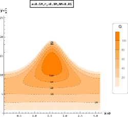
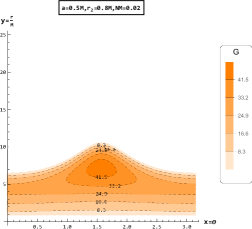
Figure 1: The above contour map representing G. Both figures assume $a=0.5M$, $r_{2}=0.8M$, and different $N$. The physical areas associated with $NM$ = 0.01 and 0.02. The transition from bottom to the top region contact with the value range of $G$.

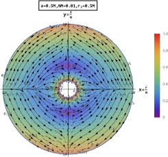
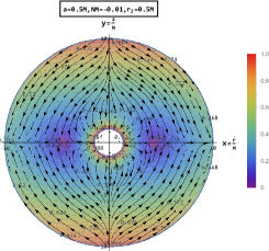
Figure 2: Two figures correspond to the streamline (solid arrow) and the isocontour (dotted line). The change in colour entirely determines the magnitudes of the three-velocity. The diagram use cylindrical-like coordinate transformation $\overline{r}=\sqrt{r^{2}+a^{2}}\sin{\theta}$, $z=r\cos{\theta}$ to make the diagram more distinct.

The streamline and isocontour diagram of the non-relativistic stiff fluid determined by equation (LABEL:42) is given by Figure 2. The isocontours of three-velocity are represented by the dashed line, the streamline is shown by the black arrow, and the stagnation point is symbolized by a blue area, so that part of the fluid flows into the black hole and others flow to the poles or the equatorial plane. From Figure 1, we chose $R=10M$ as the outer radius for investigation in the following discussion, since the timelike characteristic of velocity is assured in the interval $(r_{+},R)$. It is worth noticing that the black hole domain is symbolised by the hole in the middle, which also highlights that $\Phi$ is not well defined in the ZAMO coordinate system.

V Choked accretion

The choked accretion is a hydrodynamic mechanism that was first proposed by Hernandez, and applied to the discussion of Schwarzschild black holes and Kerr black holes Aguayo-Ortiz:2020qro ; Tejeda:2019fwr ; Aguayo-Ortiz:2019fap . The mechanism describes that perfect fluid is injected radially along the equatorial plane. If the injection velocity is too large, the anisotropic density distribution fluctuates dramatically so that part of the fluid deviates from the original orbit and is ejected along poles. This process is reversible, as seen in cases 1 and 2, respectively. We’ll focus on $N>0$ (case 1) in this section.

It was mentioned previously that to fulfill the requirements of four-velocity’s timelike character, a spherical surface with a radius of $R$ must be supplied. Physical values in the spherical shell are well-defined. At the same time, one reference point should always be established for physical quantity to be measurable. The injection rate $V_{0}$ is set at $\left(R,\frac{\pi}{2}\right)$ in equatorial plane and ejection rate $V_{ej}$ is determined at $(R,0)$ can be represented as

$$\left\{\begin{split}&V_{0}=V^{\hat{r}}\left(R,\frac{\pi}{2}\right)=\frac{\tilde{\Delta}_{0}\left(6R-6M+3r_{2}\right)N+2Mr_{+}}{\sqrt{\tilde{A_{0}}}}\\ &V_{ej}=V^{\hat{r}}\left(R,0\right)=\frac{2V_{0}\sqrt{\tilde{A_{0}}}-6Mr_{+}}{R(R+r_{2})+a^{2}},\\ \end{split}\right.$$ (49)

with

$$\left\{\begin{split}&\tilde{\Delta}_{0}=(R-r_{+})(R-r_{-})\\ &\tilde{A}_{0}=R(R+r_{2})(a^{2}+R^{2}+Rr_{2})+2MRa^{2}.\\ \end{split}\right.$$ (50)

Since the fluid is subluminal and need to ensure that flows out along both ends of the polar axis in a spherical shell, we must require $(0<V_{ej}<1)$ to acquire the range of the initial velocity $V_{0}$.

$$\frac{3Mr_{+}}{\sqrt{\tilde{A}_{0}}}<V_{0}<\frac{R(R+r_{2})+a^{2}+6Mr_{+}}{2\sqrt{\tilde{A}_{0}}}.$$ (51)

Up to now, we haven’t solved the stagnation point or the value of the coefficient $N$ in principle, thus boundary constraints must be imposed. It can be concluded from (LABEL:37) that

$$e=h\Gamma\sqrt{\frac{\tilde{\Sigma}\tilde{\Delta}}{\tilde{A}}}=h_{0}\Gamma_{0}\sqrt{\frac{\tilde{\Sigma}_{0}\tilde{\Delta}_{0}}{\tilde{A_{0}}}},$$ (52)

where

$$\left\{\begin{split}&\Gamma_{0}=\frac{1}{\sqrt{1-V^{2}_{0}}}\\ &\tilde{\Sigma}_{0}=R(R+r_{2}).\\ \end{split}\right.$$ (53)

Using the (7) and substituting (52) into (LABEL:37), we get

$$\frac{h}{h_{0}}=\frac{\rho}{\rho_{0}}=\frac{\Gamma_{0}\sqrt{\tilde{\Sigma}_{0}\tilde{\Delta}_{0}\tilde{A}}}{\Gamma\sqrt{\tilde{\Sigma}\tilde{\Delta}\tilde{A}_{0}}},$$ (54)

where density $\rho_{0}=\rho\left(R,\frac{\pi}{2}\right)$ and specific enthalpy $h_{0}=h\left(R,\frac{\pi}{2}\right)$ are determined by parameters $M$, $a$ and $r_{2}$ as the value at reference point. According to (LABEL:49), it follows that

$$N=\frac{V_{0}\sqrt{\tilde{A}}_{0}-2Mr_{+}}{\tilde{\Delta}_{0}(6R-6M+3r_{2})},$$ (55)

Simultaneously, these two equivalent conditions (45) and (55) give the location of stagnation point.

$$r_{s}=M-\frac{r_{2}}{2}+\left(\lambda-\sqrt{\lambda^{2}-\frac{\left(M^{2}-a^{2}-Mr_{2}+\frac{1}{4}r^{2}_{2}\right)^{3}}{27}}\right)^{\frac{1}{3}}+\left(\lambda+\sqrt{\lambda^{2}-\frac{\left(M^{2}-a^{2}-Mr_{2}+\frac{1}{4}r^{2}_{2}\right)^{3}}{27}}\right)^{\frac{1}{3}},$$ (56)

with

$$\lambda\equiv\frac{Mr_{+}(R-r_{+})(R-r_{-})(R-M+\frac{r_{2}}{2})}{2(V_{0}\sqrt{\tilde{A_{0}}}-2Mr_{+})}.$$ (57)

The correlation between $r_{s}$ and $r_{2}$ is depicted in Figure 3 (left) with $V_{0}=0.3,0.4,0.5$ . It is worth noting that the range selected by $V_{0}$ satisfies the constraints of (51). As the value of $V_{0}$ increases, the initial value will become smaller, and the stagnation point will show a downward trend with the increase of $r_{2}$.

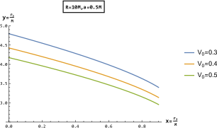
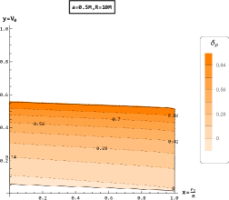
Figure 3: The stagnation point is depicted by the real line on the left with $a=0.5M$, $R=10M$ and $V_{0}=0.3,0.4,0.5$. The density perturbation colour temperature map is determined by the right.

V.1 Distribution of the density and the streamlines

Through (54) we define a quantity $\delta$ that describes the relative deviation of the ejection’s value at $\left(R,0\right)$ from the injection’s value at $\left(R,\frac{\pi}{2}\right)$, which yield

$$\delta_{\rho}\equiv 1-\frac{\rho\left(R,0\right)}{\rho\left(R,\frac{\pi}{2}\right)}=1-\sqrt{\frac{\left(1-V^{2}_{ej}\right)R(R+r_{2})\left(R(R+r_{2})+a^{2}\right)}{\left(1-V^{2}_{0}\right)\left(R(R+r_{2})(a^{2}+R^{2}+Rr_{2})+2MRa^{2}\right)}}.$$ (58)

As can be shown, the conclusion is that when $\delta_{\rho}=1$, the density of location $(R,0)$ tends to zero. When $\delta_{\rho}=0$, the density of the ejection point is equivalent to incoming point. The distribution of $\delta_{\rho}$ is given in figure 3 (right). It illustrates that the maximum value of $\delta_{\rho}$ is not greater than 1, and the entire color is homogeneous. The orange area at the bottom reveals that the injection point’s density is extremely smaller than the ejection point’s density. The density ratio approaches zero as $\delta_{\rho}$ increases in the orange area suggesting a reduced ejection rate.

Finally, we obtain a streamlined diagram that can depict the fluid’s trajectory. Applying equations (LABEL:42) to cancel time $t$ can result in

$$\alpha=\cos{\theta}\left[1+\frac{\sin^{2}{\theta}\left(r-r_{+}\right)\left(r-r_{-}\right)\left(r-M+\frac{r_{2}}{2}\right)}{2\left(r_{s}-r_{+}\right)\left(r_{s}-r_{-}\right)\left(r_{s}-M+\frac{r_{2}}{2}\right)}\right],$$ (59)

where $\alpha$ is the constant of integration. Streamlines with $|{\alpha}|=1$ are connected to the stagnation point, whereas those with $|\alpha|>1$ escape via the bipolar outflow, and the $|\alpha|<1$ area is absorbed into black hole. The streamline is described in figure 4, and the diagram(left) shows that the complete diagram is symmetrically distributed along $\theta=\frac{\pi}{2}$ (the middle solid line). The dashed line depicts the streamline’s trajectory, which differs from $|{\alpha}|$ values and represents several pathways. It is straightforward to notice that the dividing line ($|{\alpha}|=1$) explains whether fluid is absorbed into or ejected from the black hole. The streamlined diagram (right) in the cylindrical-like coordinate system ($\overline{r},z$) will be shown. Similarly, the boundary is $|{\alpha}|=1$ of the blue region generated by the dotted line.

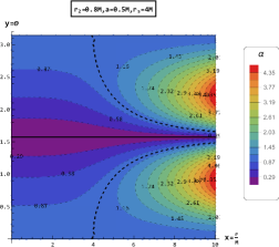
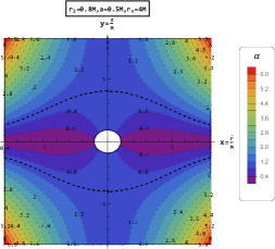
Figure 4: The parameters $r_{2}=0.8M$, $a=0.5M$ and $r_{s}=4M$ for two figures. The solid line (left) denotes $\theta=\frac{\pi}{2}$, while the dashed line reflects the isocontour line. The right side employs the coordinate transformation $\overline{r}=\sqrt{r^{2}+a^{2}}\sin{\theta}$, $z=r\cos{\theta}$, and the centre empty region represents the interior of Kerr-Sen black hole.

V.2 Injection rate, ejection rate and critical angle

The inflow and outflow should be accompanied by injection rate and ejection rate, respectively. When matched with the black hole mass accretion rate, the whole concept of choked accretion is presented. Those three rates are connected in the following way:

$$\dot{\mathscr{M}}_{in}=\dot{\mathscr{M}}+\dot{\mathscr{M}}_{out},$$ (60)

where the mass accretion rate is decided by formula (32). It can be described as

$$\dot{\mathscr{M}}=8\pi Mr_{+}\rho_{0}\Gamma_{0}\sqrt{\frac{R(R+r_{2})\tilde{\Delta}_{0}}{\tilde{A}_{0}}}.$$ (61)

It’s obvious that the accretion rate is restricted by the parameters chosen and the bounding sphere radius $R$. Now we must identify the critical angle which appears to correspond to fluid moving towards the black hole in the interval $(\theta_{c},\pi-\theta_{c})$. In this interval, the projection of the tangent vector of the streamline along the radial direction of the black hole is negative. The critical angle $\theta_{c}$ could be determined by using $V^{\hat{r}}$ in (LABEL:42). The flow is absorbed by the black hole related to $V^{\hat{r}}<0$, it follows that

$$\theta_{c}=\arccos{\left[3\left(1-\frac{2Mr_{+}}{V_{0}\sqrt{\tilde{A}_{0}}}\right)\right]^{-\frac{1}{2}}},$$ (62)

where $\dot{\mathscr{M}}_{in}$ associated with the critical angle is

$$\left\{\begin{split}&\dot{\mathscr{M}}_{in}=-2\int^{\frac{\pi}{2}}_{\theta_{c}}\rho U^{r}\tilde{\Sigma}\sin{\theta}\,\mathrm{d}\theta\,\mathrm{d}\phi=\frac{8\pi q\rho eMr_{+}}{h}=q\dot{\mathscr{M}}\\ &q\equiv\frac{2\cos^{3}{\theta_{c}}}{3\cos^{2}{\theta_{c}}-1}=\frac{\sqrt{\tilde{A}_{0}}V_{0}}{3\sqrt{3}Mr_{+}}\left(1-\frac{2Mr_{+}}{V_{0}\sqrt{\tilde{A}_{0}}}\right)^{-\frac{1}{2}},\end{split}\right.$$ (63)

Similarly, the ejection rate could be obtained $\dot{\mathscr{M}}_{out}=(q-1)\dot{\mathscr{M}}$ by using (60). The physics relating to $\dot{\mathscr{M}}_{in}=\dot{\mathscr{M}}$ is that all fluids are dragged into black hole while the critical angle $\theta_{c}=0$ $(q=1)$. The condition $\theta_{c}=0$ provides $V_{0}=\frac{3Mr_{+}}{\sqrt{\tilde{A}_{0}}}$ by (62). It shows that this is consistent with (51) restriction, it follows.

$$\dot{\mathscr{M}}_{in}=\left\{\begin{aligned} &\dot{\mathscr{M}},\quad V_{0}\leqslant\frac{3Mr_{+}}{\sqrt{\tilde{A}_{0}}}\\ &q\dot{\mathscr{M}},\quad\frac{3Mr_{+}}{\sqrt{\tilde{A}_{0}}}\leqslant V_{0}\leqslant\frac{R(R+r_{2})+a^{2}+6Mr_{+}}{2\sqrt{\tilde{A}_{0}}},\\ \end{aligned}\right.$$ (64)

and

$$\dot{\mathscr{M}}_{out}=\left\{\begin{aligned} &0,\quad V_{0}\leqslant\frac{3Mr_{+}}{\sqrt{\tilde{A}_{0}}}\\ &(q-1)\dot{\mathscr{M}},\quad\frac{3Mr_{+}}{\sqrt{\tilde{A}_{0}}}\leqslant V_{0}\leqslant\frac{R(R+r_{2})+a^{2}+6Mr_{+}}{2\sqrt{\tilde{A}_{0}}}.\\ \end{aligned}\right.$$ (65)

As $V_{0}$ range changes, $\dot{\mathscr{M}}_{in}$ steadily increases that results in a maximum value $\theta_{max}$ calculated by the formula below

$$\frac{1}{3\cos{\theta^{2}_{max}}}=\frac{R(R+r_{2})+a^{2}+2Mr_{+}}{R(R+r_{2})+a^{2}+6Mr_{+}}$$ (66)

with maximum value of injection accretion rate $\dot{\mathscr{M}}_{inmax}=q_{\max}\dot{\mathscr{M}}$, where

$$q_{\max}=\frac{2\cos^{3}{\theta_{max}}}{3\cos^{2}{\theta_{max}}-1}.$$ (67)

According to the above formula, when $R$ is large, the maximum angle $\theta_{max}\approx 54.7^{\circ}$, $q_{\max}\rightarrow\infty$ corresponds to the boundary case. To understand the transformation of accretion rate ratio, we depicts the ratio of accretion rate $\frac{\dot{\mathscr{M}}_{out}}{\dot{\mathscr{M}}_{in}}\equiv\eta$ in figure 5.

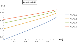
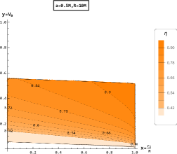
Figure 5: The left figure depicts the ratio of accretion rate as the parameter $r_{2}$ changes when $V_{0}=0.2,0.3,0.4,0.5$ are respectively fixed. The figure on the right depicts a contour map of ratios, where the upper and lower boundaries represent the range of values for $V_{0}$.

The figure above shows how $r_{2}$ influences the accretion rate ratio. When $V_{0}$ is fixed, we see that the ratio $\eta$ grows as $x$ increases. When the value of parameter $x$ is fixed in figure 5 (right), $V_{0}$ varies from the bottom boundary to the upper, and the variation range of $\eta$ is $40\%-70\%$. It can be shown that as the parameter $r_{2}$ in the Kerr-Sen black hole increases, it amplifies the ratio of ejection rate to incident rate. Consequently, this leads to a scenario where the majority of the fluid escapes from the black hole, while the inhaled fluid becomes a relatively minor component.

VI Conclusion and discussion

In this work, we first studied the choked accretion process of ultrarelativistic fluid onto axisymmetric Kerr-Sen black holes in Einstein-Maxwell-Dilation-Axion gravity. Based on solving procedure mentioned by Petrich, Shapiro, and Teukolsky, we calculated the solution describing the velocity potential field $\Phi$ of a stationary, irrotational ultrarelativistic fluid in the Boyer-Lindquist coordinates system. We discussed the analytical expression of four-velocity and converted it to the ZAMO framework to give three-velocity. The value of mass accretion rate, the energy accretion rate, and the angular momentum increase rate was also finished. We found that the angular momentum increase rate is zero, indicating that the fluid has an axisymmetric distribution $(m=0)$.

Secondly, as a result of the axial symmetry of perfect fluid and the requirement of reflection symmetry in the equatorial plane, we gave the lowest-order (2,0) solution, commonly known as quadrupolar flow. We investigated the character of quadrupolar flow and showed that one of the two constraints described is automatically satisfied, and timelike requirement of four-velocity is also solved once an appropriate region is chosen. Subsequently, we examined the correlation between dilation parameters $r_{2}$ as a function of coefficients $N$ and stagnation point $r_{s}$ in the solution, as well as the color temperature and streamlined diagrams of these regions with timelike properties.

Finally, we introduced the choked accretion model and restricted the physical region to $(r_{+},R)$ to ensure that the solution is reasonable. We also calculated the stagnation point analytic formulas based on the boundary values and drew isocontour. Within the permissible range, the initial velocity $V_{0}$ at the reference point allows us to draw a picture of its dependency on the parameters according to different colors. The connection between the density ratio of endpoint and initial point is also evaluated. We also gave the streamline diagram in cylindrical-like coordinates and discovered that the streamline associated with $\alpha\leqslant 1$ indicates that fluid is absorbed into the black hole, whereas the streamline with $\alpha>1$ represents flow ejected along poles. The injection rate and ejection rate were discussed in detail at the end of the article. The conditions for the existence of the injection rate were given and the critical angle $\theta_{c}$ during the accretion process was determined so that flow in the interval $(\theta_{c},\pi-\theta_{c})$ is sucked into black hole.

In future work, we will try to solve the choked accretion issue of curled fluid numerically and provide numerical results by merging it with the equation of motion with boundary via space-time and matter field coupling. We will consider the reaction of matter, and explore the full accretion issue using dark energy and dark matter as carriers.

- [1] Marek A. Abramowicz and P. Chris Fragile. Foundations of Black Hole Accretion Disk Theory. Living Rev. Rel., 16:1, 2013.
- [2] F. Hoyle and R. A. Lyttleton. The evolution of the stars. Mathematical Proceedings of the Cambridge Philosophical Society, 35(4):592–609, 1939.
- [3] F. Hoyle and R. A. Lyttleton. On the physical aspects of accretion by stars. Mathematical Proceedings of the Cambridge Philosophical Society, 36(4):424–437, 1940.
- [4] F. Hoyle and R. A. Lyttleton. On the accretion of interstellar matter by stars. Mathematical Proceedings of the Cambridge Philosophical Society, 36(3):325–330, 1940.
- [5] F. Hoyle and R. A. Lyttleton. On the accretion theory of stellar evolution. Mon. Not. Roy. Astron. Soc., 101:227, 1941.
- [6] H. Bondi and F. Hoyle. On the mechanism of accretion by stars. Mon. Not. Roy. Astron. Soc., 104:273, 1944.
- [7] H. Bondi. On spherically symmetrical accretion. Mon. Not. Roy. Astron. Soc., 112:195, 1952.
- [8] F. Curtis Michel. Accretion of matter by condensed objects. Astrophysics and Space Science, 15(1):153–160, 1972.
- [9] Edward Malec. Fluid accretion onto a spherical black hole: Relativistic description versus Bondi model. Phys. Rev. D, 60:104043, 1999.
- [10] E. Babichev, V. Dokuchaev, and Yu. Eroshenko. Black hole mass decreasing due to phantom energy accretion. Phys. Rev. Lett., 93:021102, 2004.
- [11] Lei Jiao and Rong-Jia Yang. Accretion onto a Kiselev black hole. Eur. Phys. J. C, 77(5):356, 2017.
- [12] Apratim Ganguly, Sushant G. Ghosh, and Sunil D. Maharaj. Accretion onto a black hole in a string cloud background. Phys. Rev. D, 90(6):064037, 2014.
- [13] Rongjia Yang. Quantum gravity corrections to accretion onto a Schwarzschild black hole. Phys. Rev. D, 92(8):084011, 2015.
- [14] Jose A. Font, Jose M. Ibanez, and Philippos Papadopoulos. Nonaxisymmetric relativistic Bondi-Hoyle accretion onto a Kerr black hole. Mon. Not. Roy. Astron. Soc., 305:920, 1999.
- [15] Rongjia Yang. Constraints from accretion onto a Tangherlini–Reissner–Nordstrom black hole. Eur. Phys. J. C, 79(4):367, 2019.
- [16] V. I. Parev. Hydrodynamic accretion onto rapidly rotating Kerr black hole. Mon. Not. Roy. Astron. Soc., 283:1264–1280, 1996.
- [17] Mikhail V. Medvedev and Norman Murray. Hot settling accretion flow onto a spinning black hole. Astrophys. J., 581:431–437, 2002.
- [18] Patrick Christopher Fragile and Peter Anninos. Tilted thick - disk accretion onto a Kerr black hole. Astrophys. J., 623:347, 2005.
- [19] Jhumpa Bhadra and Ujjal Debnath. Accretion of New Variable Modified Chaplygin Gas and Generalized Cosmic Chaplygin Gas onto Schwarzschild and Kerr-Newman Black holes. Eur. Phys. J. C, 72:1912, 2012.
- [20] Jose A. Jimenez Madrid and Pedro F. Gonzalez-Diaz. Evolution of a kerr-newman black hole in a dark energy universe. Grav. Cosmol., 14:213–225, 2008.
- [21] Haiyuan Feng, Miao Li, Gui-Rong Liang, and Rong-Jia Yang. Adiabatic accretion onto black holes in Einstein-Maxwell-scalar theory. JCAP, 04(04):027, 2022.
- [22] Loren I. Petrich, Stuart L. Shapiro, and Saul A. Teukolsky. Accretion onto a moving black hole: An exact solution. Phys. Rev. Lett., 60:1781–1784, 1988.
- [23] Lei Jiao and Rong-Jia Yang. Accretion onto a moving Reissner-Nordström black hole. JCAP, 09:023, 2017.
- [24] Rong-Jia Yang, Yinan Jia, and Lei Jiao. Exact solution for accretion onto a moving charged dilaton black hole. 12 2021.
- [25] Patryk Mach and Andrzej Odrzywo. Accretion of Dark Matter onto a Moving Schwarzschild Black Hole: An Exact Solution. Phys. Rev. Lett., 126(10):101104, 2021.
- [26] Patryk Mach and Andrzej Odrzywołek. Accretion of the relativistic Vlasov gas onto a moving Schwarzschild black hole: Exact solutions. Phys. Rev. D, 103(2):024044, 2021.
- [27] Ziqiang Cai and Rong-Jia Yang. Accretion of the Vlasov gas onto a Schwarzschild-like black hole. Phys. Dark Univ., 42:101292, 2023.
- [28] Tiziana Di Matteo, Steven W. Allen, Andrew C. Fabian, Andrew S. Wilson, and Andrew J. Young. Accretion onto the supermassive black hole in M87. Astrophys. J., 582:133–140, 2003.
- [29] Sergiy Silich, Guillermo Tenorio-Tagle, and Filiberto Hueyotl-Zahuantitla. Spherically-symmetric Accretion onto a Black Hole at the Center of a Young Stellar Cluster. Astrophys. J., 686:172, 2008.
- [30] Rodrigo Gil-Merino, Luis J. Goicoechea, Vyacheslav N. Shalyapin, and Vittorio F. Braga. Accretion Onto the Supermassive Black Hole in the High-redshift Radio-loud AGN 0957+561. Astrophys. J., 744:47, 2012.
- [31] C. Y. Kuo et al. Measuring Mass Accretion Rate onto the Supermassive Black Hole in M87 Using Faraday Rotation Measure with the Submillimeter Array. Astrophys. J. Lett., 783:L33, 2014.
- [32] Tong-Yu He, Ziqiang Cai, and Rong-Jia Yang. Thin accretion disks around a black hole in Einstein-Aether-scalar theory. Eur. Phys. J. C, 82:1067, 2022.
- [33] R. D. Blandford and D. G. Payne. Hydromagnetic flows from accretion discs and the production of radio jets. Monthly Notices of the Royal Astronomical Society, 199(4):883–903, 08 1982.
- [34] R. D. Blandford and R. L. Znajek. Electromagnetic extraction of energy from Kerr black holes. Monthly Notices of the Royal Astronomical Society, 179(3):433–456, 07 1977.
- [35] Vladimir Semenov, Sergey Dyadechkin, and Brian Punsly. Simulations of jets driven by black hole rotation. Science, 305:978, 2004.
- [36] Jonathan C. McKinney. General relativistic magnetohydrodynamic simulations of jet formation and large-scale propagation from black hole accretion systems. Mon. Not. Roy. Astron. Soc., 368:1561–1582, 2006.
- [37] Qian Qian, Christian Fendt, and Christos Vourellis. Jet Launching in Resistive GR-MHD Black Hole–Accretion Disk Systems. Astrophys. J., 859(1):28, 2018.
- [38] M. Liska, A. Tchekhovskoy, A. Ingram, and M. van der Klis. Bardeen–Petterson alignment, jets, and magnetic truncation in GRMHD simulations of tilted thin accretion discs. Mon. Not. Roy. Astron. Soc., 487(1):550–561, 2019.
- [39] X. Hernandez, P. L. Rendon, R. G. Rodriguez-Mota, and A. Capella. A hydrodynamical mechanism for generating astrophysical jets, 2011.
- [40] Emilio Tejeda, Alejandro Aguayo-Ortiz, and X. Hernandez. Choked accretion onto a Schwarzschild black hole: A hydrodynamical jet-launching mechanism. Astrophys. J., 893:81, 2020.
- [41] Alejandro Aguayo-Ortiz, Olivier Sarbach, and Emilio Tejeda. Choked accretion onto a Kerr black hole. Phys. Rev. D, 103(2):023003, 2021.
- [42] Ashoke Sen. Rotating charged black hole solution in heterotic string theory. Phys. Rev. Lett., 69:1006–1009, 1992.
- [43] Marek Rogatko. Positivity of energy in Einstein-Maxwell axion dilaton gravity. Class. Quant. Grav., 19:5063–5072, 2002.
- [44] Bruce A. Campbell, Nemanja Kaloper, Richard Madden, and Keith A. Olive. Physical properties of four-dimensional superstring gravity black hole solutions. Nucl. Phys. B, 399:137–168, 1993.
- [45] A. Garcia, D. Galtsov, and O. Kechkin. Class of stationary axisymmetric solutions of the Einstein-Maxwell dilaton - axion field equations. Phys. Rev. Lett., 74:1276–1279, 1995.
- [46] A. M. Ghezelbash and H. M. Siahaan. Hidden and Generalized Conformal Symmetry of Kerr-Sen Spacetimes. Class. Quant. Grav., 30:135005, 2013.
- [47] Canisius Bernard. Stationary charged scalar clouds around black holes in string theory. Phys. Rev. D, 94(8):085007, 2016.
- [48] David Garfinkle, Gary T. Horowitz, and Andrew Strominger. Charged black holes in string theory. Phys. Rev. D, 43:3140, 1991. [Erratum: Phys.Rev.D 45, 3888 (1992)].
- [49] José A Font. An introduction to relativistic hydrodynamics. Journal of Physics: Conference Series, 91:012002, nov 2007.
- [50] E. Babichev, S. Chernov, V. Dokuchaev, and Yu. Eroshenko. Ultra-hard fluid and scalar field in the Kerr-Newman metric. Phys. Rev. D, 78:104027, 2008.
- [51] Andrei V. Frolov and Valeri P. Frolov. Rigidly rotating zero-angular-momentum observer surfaces in the kerr spacetime. Physical Review D, 90(12), dec 2014.
- [52] Yi Liao, Xiao-Bo Gong, and Jian-Sheng Wu. Phase-transition Theory of Kerr Black Holes in the Electromagnetic Field. Astrophys. J., 835(2):247, 2017.
- [53] Vladimír Karas and Rastislav Mucha. Accretion onto a rotating compact object in general relativity. American Journal of Physics, 61(9):825–828, September 1993.
- [54] Emilio Tejeda. Incompressible wind accretion. Rev. Mex. Astron. Astrofis., 54:171, 2018.
- [55] Alejandro Aguayo-Ortiz, Emilio Tejeda, and X. Hernandez. Choked accretion: from radial infall to bipolar outflows by breaking spherical symmetry. Mon. Not. Roy. Astron. Soc., 490(4):5078–5087, 2019.