GeoDE: a Geographically Diverse Evaluation Dataset for Object Recognition

Abstract

Current dataset collection methods typically scrape large amounts of data from the web. While this technique is extremely scalable, data collected in this way tends to reinforce stereotypical biases, can contain personally identifiable information, and typically originates from Europe and North America. In this work, we rethink the dataset collection paradigm and introduce GeoDE , a geographically diverse dataset with 61,940 images from 40 classes and 6 world regions, and no personally identifiable information, collected through crowd-sourcing. We analyse GeoDE to understand differences in images collected in this manner compared to web-scraping. Despite the smaller size of this dataset, we demonstrate its use as both an evaluation and training dataset, allowing us to highlight shortcomings in current models, as well as demonstrate improved performances even when training on the small dataset. We release the full dataset and code at https://geodiverse-data-collection.cs.princeton.edu/

1 Introduction

The creation of large-scale image datasets has enabled advances in the performance of computer vision models. Although previously limited by manual collection and annotation efforts [12, 14, 11], recently the size of these datasets has rapidly grown. This growth has been empowered by a new data collection framework: scraping web images at scale. These images are either human-labelled (e.g., ImageNet [8, 22]), use tags (e.g., CLIP-400M [20]) or used for self-supervised learning (e.g., PASS [2]).

GeoYFCC distribution [9]

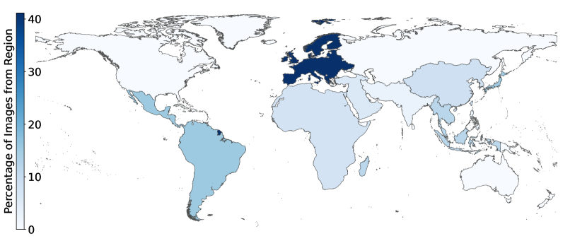
GeoDE distribution (ours)

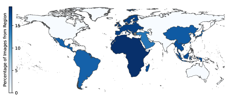
Figure 1: We construct a geographically diverse dataset GeoDE that is approximately balanced across 6 world regions. We visualize the images per region, and compare our distribution (bottom) to that of a previously created diverse dataset GeoYFCC [9] (top).

However, these web-scraped datasets come with their downsides. One of these downsides is that these datasets can often contain pernicious gender and racial biases by underrepresenting certain demographic groups and using stereotypical depictions of these groups [4, 33, 29]. In this work, we consider the aspect of geographic bias. Works like Shankar et al. [23] and de Vries et al. [7] show that these datasets consist of images mostly from North America and Western Europe. Moreover, this lack of geo-diversity propagates into downstream recognition tasks–resulting in difficulty in recognizing common household objects from non-Western regions.

Dataset	Size; distribution	Collection process; annotation process	Geographic coverage	Personally Identifiable Info (PII)
ImageNet [8, 22]	14.2M images; mostly balanced across classes	Scraped images from the web based on the class label; crowd-sourced annotations	Mostly North America and Western Europe [23]	Contains people, some images have faces blurred [32]
grayOpenImages [17]	9.1M images; long-tailed class distribution	Flickr images with CC-BY licenses; automatic labels with some human verification	Mostly North America and Western Europe [23]	Contains people
OpenImages Extended [1]	478K images; long-tailed class distribution	Crowd-sourced gamified app to collect images; automatic labels and manual descriptions	More than $80\%$ of images are from India	People are blurred
GeoYFCC [9]	330K images; long-tailed class distribution	Flickr images subsampled to be geodiverse; noisy tags	Geographically diverse (62 countries), but concentrated in Europe	Contains people
PASS [2]	1.4M images; N/A (no labels)	Random images from Flickr; no annotations	Collected from Flickr, thus mostly North America and Western Europe	No people
DollarStreet [21]	38,479 images; mostly balanced across topics	Images by professional and volunteer photographers; manual labels including household income	63 countries in four regions (Africa, America, Asia and Europe)	Yes, with permission
GeoDE (ours)	61,940 images; balanced across classes&regions	Crowd-sourced collection using paid workers; manual annotation	Even distribution over six geographical regions (Tab. 3)	No identifiable people and no other PII

Table 1: We compare recent approaches to dataset collection, along with the distribution and sizes of each. Although GeoDE is smaller than recent datasets, we ensure that the images are sourced with permission of the creator, contain no identifiable people, and are balanced across both regions and object classes.

In this work, we construct a new dataset that allows us to both expose these geographic biases, as well as train models to perform better across different geographic regions. We do so using a unique approach: rather than improving web-scraped datasets (as has been attempted in the past [9]) or curating available household images (as in [21]), we explore a data collection approach where we collect images via crowd-sourcing. We commission photos of different objects from people across the world. This approach allows for a much tighter control of image distribution. We partnered with a company called Appen (www.appen.com) and crowd-sourced the Geographically Diverse Evaluation (GeoDE) dataset. GeoDE contains 61,940 images roughly balanced across 40 object categories and six geographic regions. Despite the comparatively small size of GeoDE, the dataset has several key advantages.

First, the object recognition problem becomes surprisingly challenging since the images represent the diverse appearance of common objects across six global regions: Africa, the Americas, East Asia, Europe, Southeast Asia, and West Asia. Similar to de Vries et al. [7], we show that modern object recognition models perform poorly on recognizing objects from Africa, East Asia, and SE Asia. Augmenting current training datasets (like ImageNet [8, 22]) with images from GeoDE yields an improvement of 9.0% on DollarStreet [21] and 20.9% on a test split of GeoDE .

Second, requesting images containing specific object classes removes selection bias: objects present in images that are web-scraped are uploaded by creators with different incentives, e.g. to make exciting/unique content or to generate engagement [24], and disincentives showing mundane everyday content. We show that the distribution of images in GeoDE is different to that in other datasets, even when controlling for world region and object class.

Third, we own the copyright to all of the images in GeoDE , have explicit permission from content creators to use these images for machine learning applications, and ensured fair compensation to the content creators.

2 Related Work

There are three key research directions that inspired this work. The first is the call to increase geographic diversity in visual datasets [23, 7]. In response, there have been attempts to construct geographically diverse datasets [21, 9, 1], summarized in Sec. 1. However, these datasets are still geographically concentrated (in Europe for GeoYFCC [9], India for OpenImages Extended [1]), and/or are still relatively small scale (DollarStreet [21]), prompting our work.

Second, in using crowd-sourcing to generate visual content rather than using web-scraped images, we follow recent video datasets Charades [24], Epic Kitchens [6] and Ego4d [13]. However, we differ in that our key goal is to ensure a geographically balanced dataset. This poses challenges in recruitment and dataset scope (more in Sec. 3).

Finally, in our data collection efforts we take into account the extensive literature around selection bias in computer vision datasets [27, 4, 33, 29, 25, 10, 31, 3] and ensure that our dataset is collected responsibly, with attention to privacy, consent, copyright and worker compensation [3].

3 Collecting GeoDE

We describe our data collection process, including our selection of object classes and world regions.

Selecting the object classes. We focus on object classes that are likely to be visually distinct in different parts of the world. Selecting such objects is a chicken-and-egg problem: without a geographically diverse dataset at our disposal, it is unclear which objects are diverse. We adopt a number of heuristics using existing datasets to find a plausible set. The full process is detailed in the appendix, but briefly, we use simple computer vision techniques (linear models and visual clustering, using features extracted from self-supervised PASS-pretrained models [2]) along with manual examination to identify a set of candidate tags from DollarStreet [21] and GeoYFCC [9] (e.g., “chili,” “footstool,” “stove”). To prune these tags, we remove those that are not objects (e.g., “arctic”, “descent”), removing wild animals not found in all regions (e.g., “gnu”, “camel”) and group variants of objects (e.g., “stupa”, “temple”, “church”, “mosque” and “chapel”). The final set of objects is in Tab. 2.

Indoor common	bag, chair, dustbin, hairbrush/comb, hand soap, hat, light fixture, light switch, toothbrush, toothpaste/toothpowder
Indoor rare	candle, cleaning equipment, cooking pot, jug, lighter, medicine, plate of food, spices, stove, toy
Outdoor common	backyard, car, fence, front door, house, road sign, streetlight/lantern, tree, truck, waste container
Outdoor rare	bicycle, boat, bus, dog, flag, monument, religious building, stall, storefront, wheelbarrow

Table 2: GeoDE consists of 40 object classes, loosely organized into 4 groups.

West Asia	Saudi Arabia, United Arab Emirates, Turkey
Africa	Egypt, Nigeria, South Africa
East Asia	China, Japan, South Korea
SE Asia	Indonesia, Philippines, Thailand
Americas	Argentina, Colombia, Mexico
Europe	Italy, Romania, Spain, United Kingdom

Table 3: GeoDE consists of images from six world regions. Within each region, there are 3-4 countries contributing to most of the images, chosen to balance the diversity of the images against practical data collection considerations. Participants from outside these countries but within the same region were still accepted.

Selecting diverse geographic regions. We chose six regions across the world: Africa, Central and South America (“Americas”), East Asia, Europe, Southeast Asia and West Asia. Within each region, we targeted 3-4 countries (Tab. 3). These were chosen due to the lack of available images from these regions in most public datasets [23, 7, 30]; the countries were chosen based on the presence of participants within Appen’s database. We obtain a roughly even distribution of images across each class and region pair.

Image collection and worker demographics. Workers were asked to upload images for a given object class, following the instructions in Fig 2. There were more than 4,500 workers, representing a range of genders, ages and races (Fig. 3). All images submitted were manually checked by Appen’s quality assurance (QA) team.

General Instructions
In this task, you will submit up to 3 photos of the same type of object (e.g., upload 3 photos of 3 different bags; please do not upload 3 photos of the same bag from different angles). 1. Please make sure the location function is enabled for the camera. 2. The photo resolution should be at least 640 x 480. 3. All images should be new photos captured with
Appen Mobile. 4. Please make sure it’s a single object per image. 5. Please make sure it’s a well-lit environment and the object is clearly visible in the photos. 6. Please make the object occupy at least 25% of the image. 7. Objects captured are foregrounded and not occluded. 8. Objects should not be blurred, e.g., motion blur. 9. No effects or filters added (cropping is acceptable). 10. Please try to avoid capturing people in the images (it’s OK if people are blurry in the background and far from the camera). 11. Please try to avoid capturing vehicle license plates in images.

Figure 2: Image collection instructions given to workers.

Figure 3: Demographics of workers contributing images.

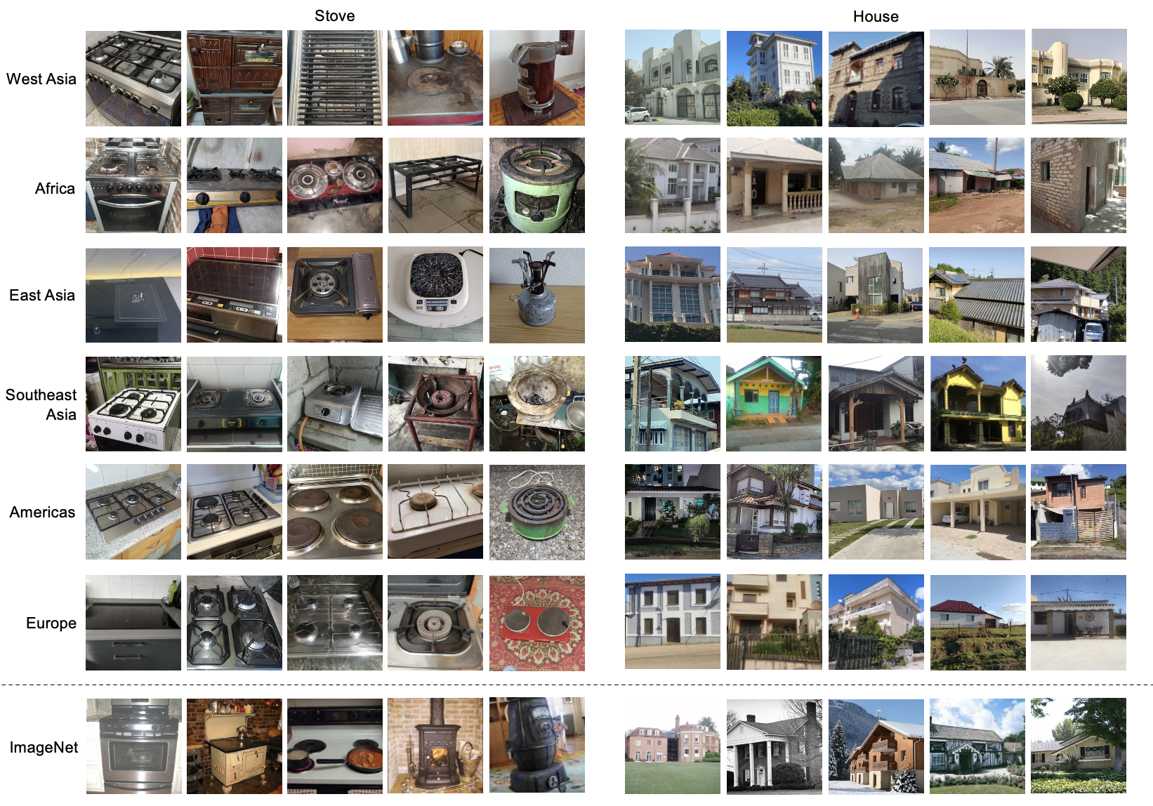
Figure 4: Sample images of two object classes in different regions within GeoDE (and ImageNet in the bottom row, for comparison). Note the variety of stoves and houses across geographic regions in GeoDE – and also the fact that the stoves are more used (thus arguably more realistic) than in ImageNet. Product labels on images have been blurred.

Lessons learned from collecting GeoDE . When collecting images for GeoDE, we additionally wanted to understand if crowd-sourcing images was a viable method to collect datasets. Some challenges we faced were in finding the right language to use to define an object: “stove” was originally underrepresented until the definition of “stove” was clarified to “any cooking surface either electric, gas, induction.”, and removing multiple copies of the same image. Other than these, we found that the collection process went smoothly. Following instructions, only 0.78% images contained identifiable information. Some images contain non-identifiable incidental people in the background (especially for larger object classes, like “monument”).

The chief downside with such a data collection process is the large cost: each image cost $1.08 (not including researcher time). This allowed us to fairly compensate workers for their labour as well as the QA team to ensure the quality of these images. This limited the size of the dataset; however, despite the small size, in the following sections we highlight the applicability of GeoDE. Our hope is that seeing the benefits of GeoDE will encourage the computer vision research community (which already spends significant resources on data collection) to reroute more of those resources towards more geographically-diverse and representative datasets (with fair worker compensation).

4 Comparing GeoDE to current datasets

We compare GeoDE with three datasets: the canonical ImageNet [8], the more geographically diverse (but still webscraped) GeoYFCC [9] and finally, the recently curated DollarStreet dataset [21].

Qualitative. In Fig. 4, we show a subset of 60 GeoDE images of “stoves” and “houses” (more in the appendix). Compared to images from ImageNet, we see a larger variety of stoves: e.g., induction coils, single and two burner stoves. The stoves also appear more used than those in ImageNet. Similarly, for “house,” we see a larger range in terms of materials used and size. In the Secs. 5 and 6 we examine the impact of this diversity on visual recognition models.

Statistics. GeoYFCC is a webscraped dataset subsampled from YFCC100M [26] to be geographically diverse; thus, not surprisingly, by raw counts it is a much larger dataset compared to both DollarStreet and GeoDE, with over 1M images orginating from 62 countries. However, looking at the regions (Fig. 1) reveals imbalances: most of the countries are from Europe. Moreover, this dataset does not have curated labels, just tags, and the distribution among tags is also long-tailed (the top 20 out of 1197 tags take up 34% of the dataset). Comparatively, GeoDE is balanced across both regions and classes. DollarStreet [21] is a much smaller dataset (38,479 images, averaging 133 images per each of 289 classes) of photos taken by volunteer photographers. For a fairer comparison to GeoDE, we consider the 40 most common classes in DollarStreet; DollarStreet has, on average, 382 images for each of these, while GeoDE has on average 1548 for each of its 40 classes.

	West Asia	Africa	East Asia	Southeast Asia	Americas	Europe
Plate of food
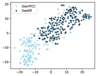
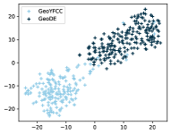
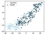
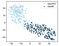
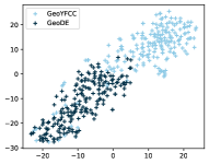
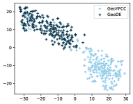
Storefront

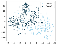
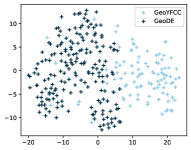
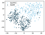
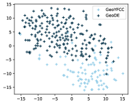
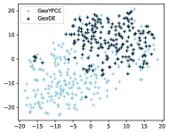
Figure 5: We visualize the TSNE plots for several of object classes per region for GeoYFCC (light blue) and GeoDE (dark blue). While the features do overlap slightly, on the whole, they are very different for dataset distributions, even within each (region, object) tuple.

Object appearance. Finally, we take a stab at quantifying the differences in the appearance of images collected through crowd-sourcing and web-scraping, by comparing the images in GeoDE with those in GeoYFCC [9] and DollarStreet [21]. We extract features for each dataset using a ResNet50 model [16] trained with self-supervised learning SwAV [5] on the PASS dataset [2]. We first train linear classifiers to predict which dataset an image was drawn from. Quite surprisingly, the classifier achieves an accuracy of 96.3% when trying to distinguish between GeoYFCC and GeoDE, and an accuracy of 96.1% when trying to distinguish between DollarStreet and GeoDE. However, this could be the result of having different distributions of regions (in the case of GeoYFCC) and different objects (for both). To understand how the dataset distributions are different beyond just the class/region frequencies we obtain low-dimensional TSNE embeddings [28]. For each dataset, we consider images that are within a certain region and contain an object and visualize how the distributions differ from GeoDE (Figs. 5 and 6). For both datasets, we do see some difference between the feature distributions, however, this is much more pronounced for GeoYFCC, possibly due to effects of webscraping.

	Africa	Americas	Europe
Cooking pot
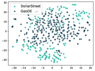
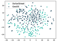
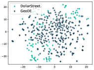
Plate of food
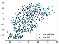
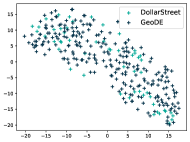
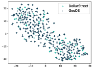
Stove

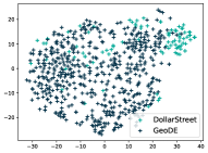
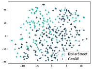
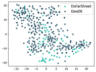
Figure 6: We visualize the TSNE plots for several of object classes per region for DollarStreet (cyan) and GeoDE (dark blue). We see that these features overlap significantly more than that of GeoYFCC, however, there are still objects with different distributions (e.g. “Stove” in Americas).

Relative value of an image. Similar to the canonical work on dataset bias [27], we measure the relative value of an image from GeoDE and DollarStreet. That is, we measure the number of training images needed for strong cross-dataset generalization. Concretely, we select 13 classes from DollarStreet which (1) appear in GeoDE, and (2) have more than $100$ images. We restrict both datasets to these 13 classes, resulting in $4,788$ images for DollarStreet and $17,245$ images for GeoDE. We now extract features using a PASS trained network, and train linear models to predict the 13 classes. First, we train a baseline model on 250 randomly sampled DollarStreet images and evaluate it on the remaining DollarStreet images; we then train models with increasing numbers of images from GeoDE until we match the accuracy of the DollarStreet-trained baseline. This occurs with 3,000 GeoDE training images. Next, we do a similar process for a baseline trained on 250 randomly sampled GeoDE images. However, we are unable to match its accuracy on GeoDE using DollarStreet training images, even after using all $4,788$ images of these classes, showing a higher relative value per image in GeoDE .

5 GeoDE as an evaluation dataset

lightswitch	bus	chair	bag	dog	monument	car	hairbrush	boat	cooking pot	hat	road sign	bicycle	religious bld	flag	toothbrush	toothpaste	storefront	wheelbarrow	light fixture	truck	plate of food	hand soap	front door	jug	stove	lighter	stall	streetlight	fence	backyard	toy	candle	waste cont.	tree	house	spices	clean. equip.	medicine	dustbin
98	97	97	96	96	96	96	95	95	95	93	93	92	92	91	90	90	89	89	88	88	88	86	85	85	78	77	76	76	75	74	73	71	69	68	63	63	59	54	37

Table 4: Per-class accuracy (in %; decreasing order) of CLIP [20] on GeoDE. Objects in bold are poorly recognized.

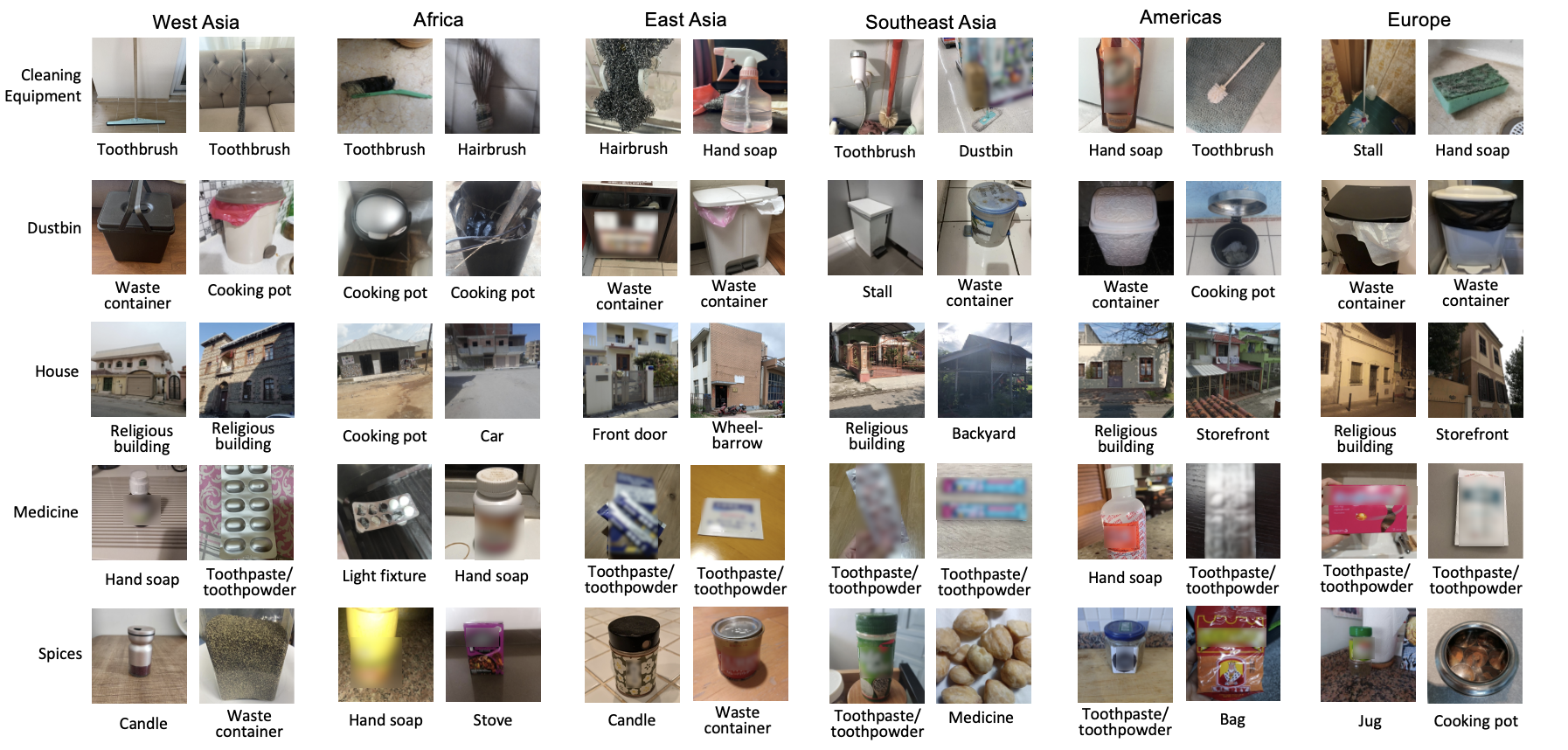
Figure 7: Example errors that the CLIP [20] model makes on GeoDE images (the ground truth label on the left, CLIP prediction at the bottom). There are some systematic errors, e.g., classifying “house” as a “religious building”, particularly on images from regions in Asia. (product labels on images have been blurred. )

spices	stove	religious building

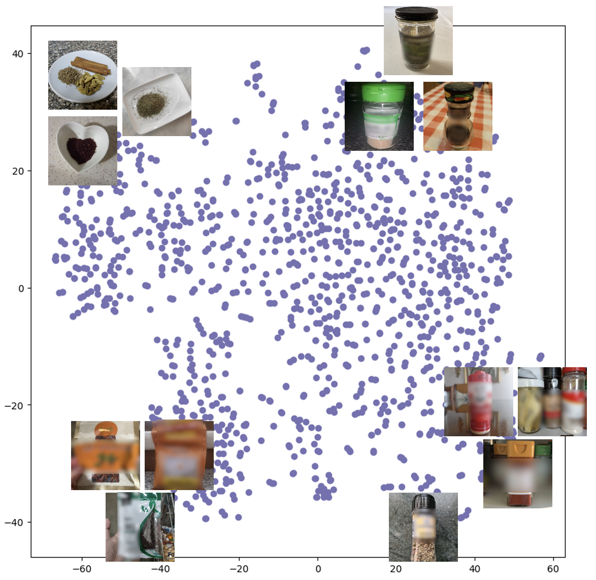
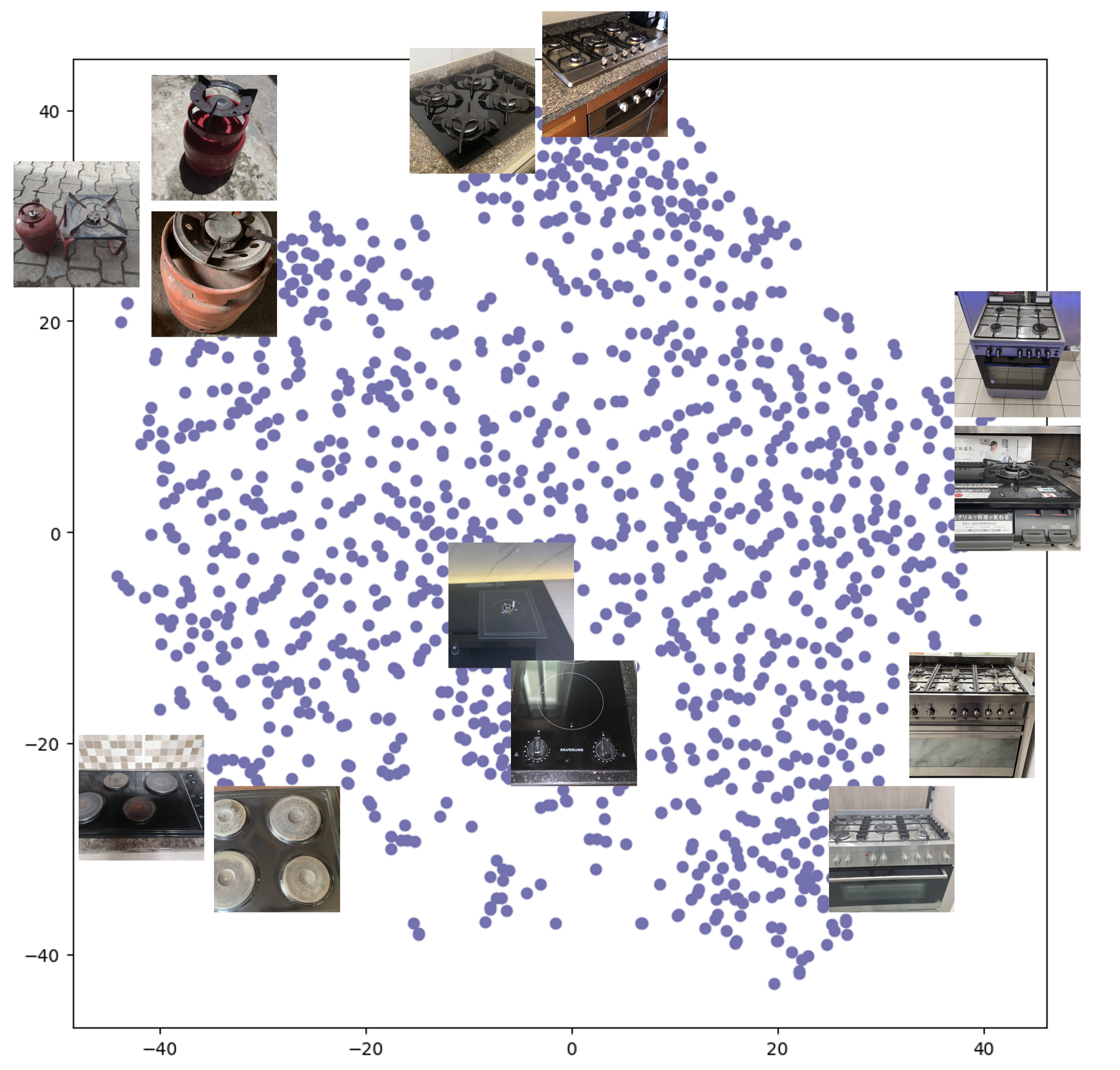
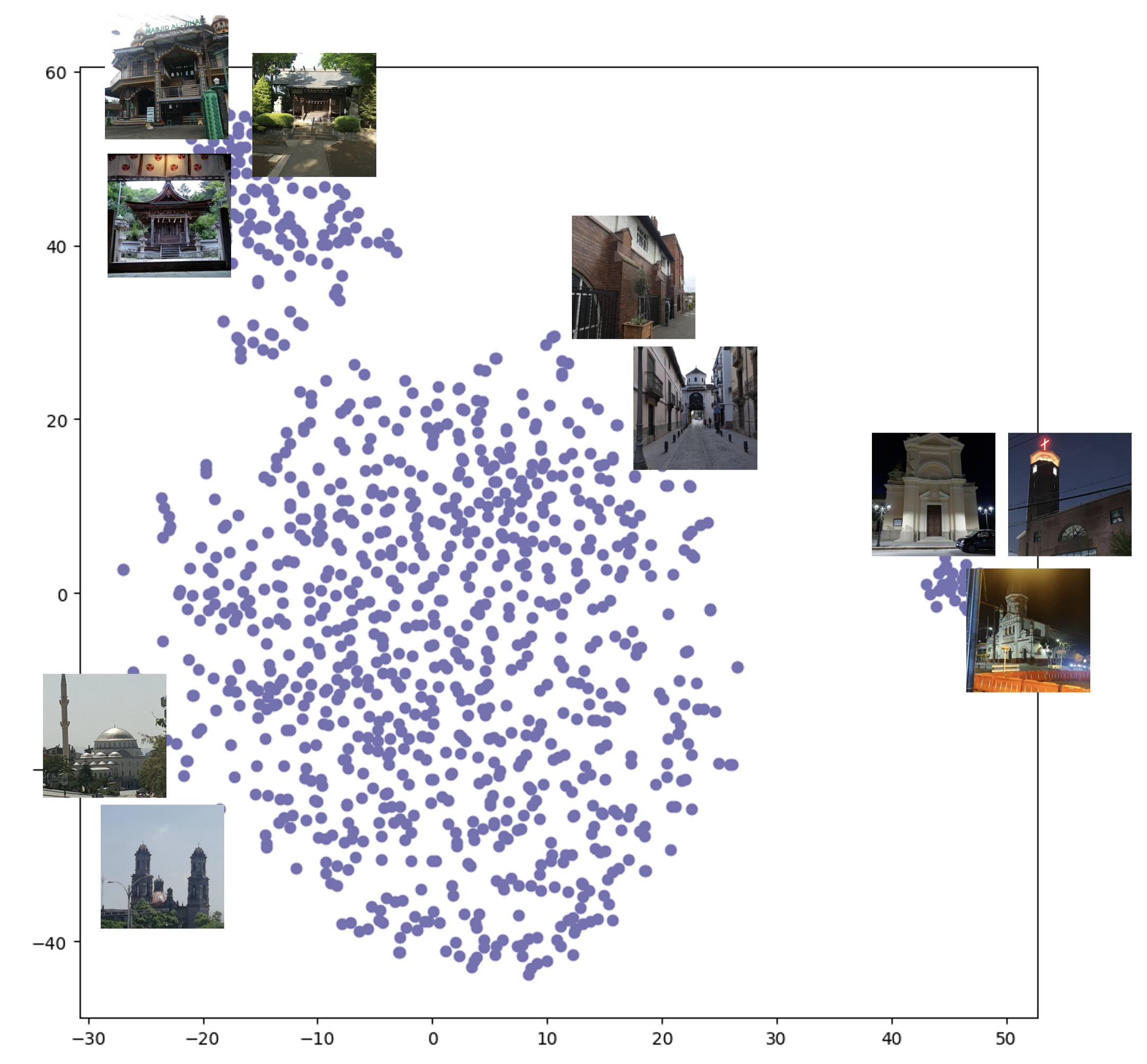
Figure 8: We show the TSNE plots of classes which have large regional disparities in accuracy from the CLIP trained model and show images from different parts of the plots. For “religious buildings”, we see that GeoDE contains a cluster of monasteries and temples, mostly from East and Southeast Asia. For “spices”, we see a separation based on the container.

We now analyze the use of GeoDE as an evaluation dataset, by using it to evaluate two canonical models: the recent CLIP [20] and an ImageNet [8]-trained model.

Implementation details. For the CLIP model, we use the weights provided for the ViT-B/32 model. We use text prompts for all 40 object categories as described in the zero-shot recognition setup of [20]. To train a model on ImageNet [8], we first match the classes of GeoDE and ImageNet. We find the corresponding synset for each GeoDE class in WordNet [18], and include all images of that synset and its children. For two object categories (“backyard” and “toothpaste/toothpowder”) we do not find any matching categories, and so we ignore these categories in the quantitative analysis. We split our filtered ImageNet [8] dataset into train (38,353 images), validation (12,794 images), and test (12,795 images) datasets. As in Sec. 4 we extract features using a ResNet50 model [16] trained with self-supervised learning SwAV [5] on PASS [2], and retrain the final layer.

Results. Tab. 5 shows the accuracy across different regions on these two models. Both models perform the best on images from Europe and the worst on images from Africa (difference of more than 7% in both cases). Tab. 4 further breaks out the per-object accuracy for CLIP. While the average accuracy is 82.8%, classes like “dustbin” (37.3%), “medicine” (54.1%), “cleaning equipment” (59.0%) and “spices” (63.2%) perform poorly. Fig. 7 shows example errors.

Model	WAsia	Africa	EAsia	SEAsia	Americas	Europe
ImageNet	69.4	62.7	63.3	67.3	68.6	69.9
CLIP	84.0	78.7	79.9	81.9	84.4	85.8

Table 5: Accuracies (in %) on GeoDE of a model trained on a subset of ImageNet [8] (details in Sec. 5) and of CLIP [20]. The models perform best on images from Europe, and worst on images from Africa.

In seeking to understand whether the accuracy variation might be explained by the differences across geographic regions, we compute the minimum and maximum per-region accuracy for each object (Fig. 9). We also compute the confidence interval for the expected distribution of per-region accuracy for each object based on the object’s overall accuracy (by drawing 500 random partitions of the images into the 6 regions, and computing the resulting per-region accuracies.) We find that 31 of 40 objects have a minimum and/or maximum region accuracy that falls outside the corresponding 95% confidence interval, suggesting that these objects (including for example “house” “dustbin”, and others) exhibit significant geographic variation (at least with respect to the visual distribution learned by CLIP).

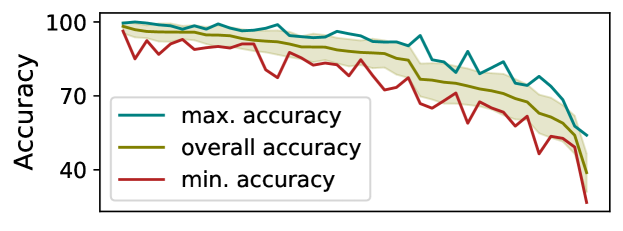
Figure 9: We compute the maximum and minimum accuracy of CLIP [20] for each object across the 6 geographic regions in GeoDE. The objects are on the x-axis, sorted by overall accuracy. We find that 31 of 40 objects have at least one region whose accuracy falls outside the 95% confidence interval (computed based on the overall accuracy), suggesting that significant differences across the regions.

Zooming in on the individual object classes, we note some interesting qualitative findings. For example, “fence” is over 88% accurate for images from Europe, but only 60% and 59% for images from Africa and Southeast Asia respectively. Similarly, “stove” has accuracy of 95% in the Americas but only 67% in East Asia. We visualize this using the TSNE plots of the features for these classes in Fig. 8, and note that these objects are region specific. For example, “religious buildings” from East and Southeast Asia can include buildings like monasteries and temples. Similarly, single- and two-burner “stoves” are primarily from countries in Africa and Southeast Asia.

6 Impact of training with GeoDE

Finally, we attempt to answer how training with GeoDE data can improve the performance of models pre-trained on large-scale web-scraped data. Concretely, we investigate training a model where we combine images from GeoDE with images from ImageNet. We find the combination of the two can improve results across regions.

6.1 Training a model with GeoDE

We would like to understand how training a model with data from GeoDE affects the object recognition capabilities of the dataset. Fixing the total number of images used for training, we train a linear model, using a pre-trained feature extractor, on a dataset comprised entirely of ImageNet images and a dataset comprised of both ImageNet and GeoDE images. The feature extractor is a ResNet50 [15] model trained on PASS [2] using SwAV [5] .

Implementation details. We split the GeoDE dataset into a train (4,970 images per region), validation (between 1657 and 2188 images per region), and test (between 1657 and 2189 images per region) datasets. We use the validation dataset to select training hyperparameters. We consider the training set for our ImageNet only model as the same 38,353 image training set constructed in Sec. 8, only considering tags in ImageNet that correspond to classes within GeoDE. To construct the training set of our ImageNet and all regions in GeoDE model, we start with the training set for ImageNet and add in the training sets for all 6 regions in GeoDE while removing proportionately per class the same number of images from ImageNet. This procedure gives a training set of 29,820 GeoDE images and 8,533 ImageNet [8] images. The final models are trained using an SGD optimizer, with a learning rate of 0.1, and momentum of 0.9, for 500 epochs with cross entropy loss. We use models with the highest accuracy on the validation set. Unless specified otherwise, results are reported on the test set.

Results. We first report results on the GeoDE test set, and notice a significant improvement in accuracy across all regions, as a result of training with both GeoDE and ImageNet (Tab. 6). However, this improvement could come from the ImageNet + GeoDE dataset matching the domain of the GeoDE evaluation set and may not generalize to other datasets. To address this, we also test these models on a different dataset: the DollarStreet dataset [21]. This dataset has been used before as an evaluation benchmark [7], to understand if current object recognition models can perform well on objects from a diverse set of regions. Tab. 7 lists the per class accuracies for the object categories that overlap between GeoDE and DollarStreet. We see an increase in performance across most categories, suggesting that GeoDE is more geo-diverse than ImageNet and that there is an advantage to using geo-diverse data in the training set.

Model	WAsia	Africa	EAsia	SEAsia	Americas	Europe	Avg
ImageNet	69.4	62.7	63.3	67.3	68.6	69.9	66.9
+GeoDE	88.2	86.7	86.4	86.5	89.1	90.0	87.8

Table 6: We see significant improvements on GeoDE after augmenting ImageNet with images from GeoDE .

	bicycle	chair	clean.equip	cooking pot	dustbin	hand soap	house	light fixture	light switch	medicine	plate of food	stove	toy	Average
ImageNet	92	86	19	49	76	49	88	36	77	80	84	89	50	60
+GeoDE	95	88	36	61	68	65	91	63	79	78	96	85	58	69

Table 7: We compare the per class accuracies of the DollarStreet [21] dataset for a model trained on only ImageNet [8] and a model trained on both ImageNet and GeoDE . We find that adding GeoDE into the training pipeline can improve the overall performance of the model.

6.2 Cost-vs-Diversity tradeoffs

The main drawback of GeoDE is the cost of this dataset: images collected in this way cost more than the standard pipeline of web-scraping and crowd-sourcing annotations. Thus, it is important to identify which classes and regions contribute most to the overall model. To investigate this, we start with the filtered ImageNet dataset described above, vary the amount of GeoDE data from a particular region, and analyze the change in overall regional performance and regional performance for specific objects.

Implementation Details. We start with a dataset fully comprised of the 38,353 filtered ImageNet images. We add a region of GeoDE’s data back into the dataset and remove the same number of ImageNet images to keep the number of images and class balance the same. Other training details remain the same as in Sec. 6.1.

Evaluation. As we are evaluating on the GeoDE test set, there are two possible sources of performance gain: (1) the model is able to take advantage of the additional regional information from the GeoDE data; and (2) the GeoDE images were collected using the same collection method as the test set and from Sec. 4, we saw that there is a difference in the feature space that can be attributed to the collection method itself (crowd-sourcing rather than web-scraping). In order to distinguish between these two sources, we measure the accuracy on both the region in the train set and accuracy on the images from Europe. We also measure the increase in AP for specific objects to better understand which objects benefit most from GeoDE data.

Results. We find that the performance both within each specific region and in Europe increase with the additional GeoDE data. The relative increase in performance for the specific region (i.e. Africa or Southeast Asia) is larger than the increase for Europe, showing the value of data for each region, moreover, the improvements do not saturate, suggesting that more data could lead to further gains. Full results are presented in the supp. mat. We also examine the classes that have the largest increase in average precision (AP) as the regional GeoDE images are added to the dataset in Figure 10. We present the object classes that see the most improvement in Tab. 8. In general, we see a large overlap in which objects benefit the most from regional GeoDE data. In particular, the performance on “spices”, “waste container” and “cleaning equipment” see large improvements in AP across all regions.

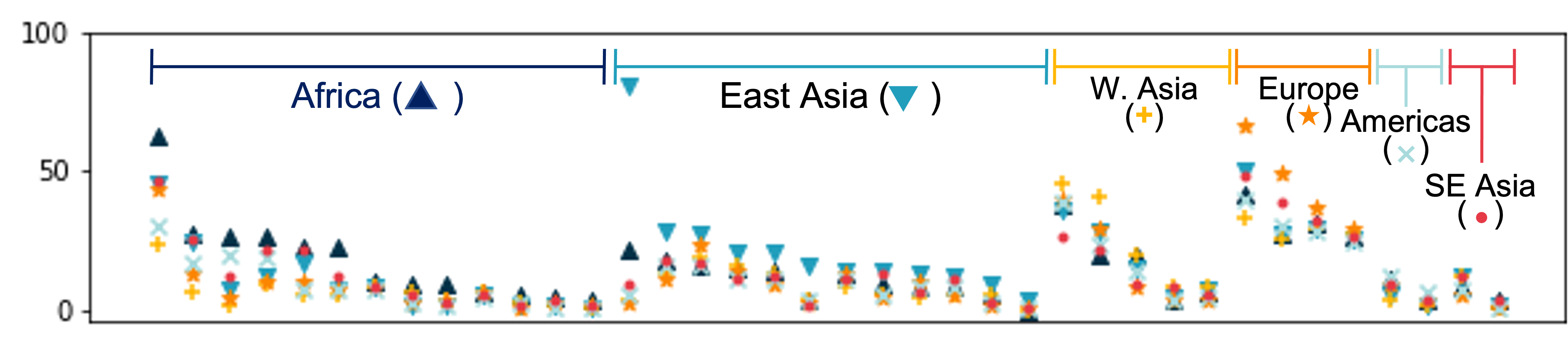
Figure 10: We measure the relative improvement in AP per object when GeoDE images from that region are included in training. Each vertical line represents an object, and we sort them by the region where that object saw the largest improvement. We see that Africa and East Asia see the largest improvement for the most classes.

Region	Classes with largest percent increase in AP
Africa	waste cont., spices, dustbin, clean. equip., hand soap
Americas	dustbin, spices, clean. equip., medicine, waste cont.
E. Asia	relig. blg., spices, dustbin, waste cont., clean. equip.
SE. Asia	waste cont., spices, medicine, clean. equip., dustbin
W. Asia	dustbin, hand soap, clean. equip., spices, jug

Table 8: We highlight the classes with the largest increases in the AP when adding in training images from GeoDE.

7 Conclusions

We have introduced a new dataset, GeoDE , which uses crowd-sourcing for image collection, a significant departure from the popular computer vision dataset collection paradigm of web-scraping for image collection. Through this collection method, we ensured that this dataset does not contain personally identifiable information, that we own the rights to the images, that the image creators were compensated for their work, and we are able to control for geographic diversity and object distribution in the dataset. We show that GeoDE is a useful dataset for evaluating and highlighting shortcomings in common models (e.g. CLIP) and can also improve performance when added to the training dataset. Additionally, the GeoDE dataset shows that crowd-sourcing is a viable image collection technique for creating diverse and responsible image datasets.

Acknowledgements. This material is based upon work partially supported by the National Science Foundation under Grant No. 2145198. Any opinions, findings, and conclusions or recommendations expressed in this material are those of the author(s) and do not necessarily reflect the views of the National Science Foundation. We also acknowledge support from Meta AI and the Princeton SEAS Howard B. Wentz, Jr. Junior Faculty Award to OR. We thank Dhruv Mahajan for his valuable insights during the project development phase. We also thank Jihoon Chung, Nicole Meister, Angelina Wang and the Princeton Visual AI Lab for their helpful comments and feedback during the writing process.

Here, we provide some more details about our experiments.

• In Sec A, we describe our heuristic to select object categories in more detail.

• In Sec B, we compare the GeoDE feature space to that of ImageNet [8]

• In Sec. D, we provide results when finetuning pre-trained models rather than just training the final layer of a ResNet.

• In Sec. E, we give more details about GeoDE , including the counts of images of different regions and categories, as well as more sample images from this dataset.

Appendix A Selecting object categories for GeoDE

In this section, we provide more details about the object selection heuristic we employed. We mainly used the GeoYFCC [9] dataset that was constructed to be geodiverse.

Implementation details. Features for GeoYFCC were extracted using a ResNet50 [15] pretrained on ImageNet [8]. We used Logistic regression, Linear SVM and KMeans clustering implementations from the sklearn library [19]. We used continents as regions. GeoYFCC [9] contains over 1200 tags, we ignored all tags with counts in the bottom 20th percentile, giving us a total of 745 tags.

First, we apply each of these methods to GeoYFCC to identify candidate tags.

• For each region $R$, we train a linear model using a feature extractor and images from all regions except $R$ and a linear model trained on all images from all regions, to predict the presence or absence of each tag. We then applied both models to images from $R$. The difference in performance between these models allows us to measure the difference in appearance of the tag. We selected tags where in the weighted average precision on the region was less than 0.8* the performance on other regions. This gave us a set of 277 tags such as “footstool”, “chili”, “case”, etc.

• For each tag $T$, we train a linear SVM to predict the region given the features of images containing tag $T$. If this model has high accuracy, this suggests that this tag is visually different across regions. We selected tags that had an accuracy of over 50%. 223 tags were identified in this manner. “Cork”, “bowler_hat” and “mountain_bike” are examples of tags found in this way.

• We clustered features of images containing tag $T$. We then computed the Gini impurity of each world region, and selected tags that had a median Gini value of at least 0.5. This gave us 75 tags in total. Examples of tags found in this way were “chili”, “footstool” and “stove”.

Leave one out training
curler, fan, footstool, chili, coconut, toilet, canoe, motorboat, mountain-bike, stupa, villa, backpack, baseball-glove, basin, basket, bat, bathtub, battery, beer-mug, belt, blade, bowl, bowl, broom, bucket, carryall, case, cash-machine, cassette, cleaver, cologne, cooler, counter, dinner-dress, dinner-jacket, dish, gown, grille, hammer, jacket, kettle, microphone, parka, porch, rack, remote-control, sandal, scale, shelf, shot-glass, stereo, stocking, stool, sweater, tape, teddy, timer, tripod, trouser, turntable, wardrobe, weight, wok, woodcarving, hot-pot, chewing-gum, cucumber, lime, fig, pineapple, jackfruit, kiwi, mango, basil, garlic, sage, lager, ale, porter, stout, champagne, rum, tequila, vodka, whiskey, mocha
Linear SVM for region
mountain-bike, bicycle, raft, ferry, ship, kayak, streetcar, bus, impala, car, footstool, bench, chair, mushroom, breakfast, vegetable, dessert, dinner, door, bowler-hat, house, building, chandelier, lamp, light, castle, acropolis, fortress, tower, palace, dome, architecture, memorial, statue, sculpture, gravestone, arch, temple, stupa, monastery, church, cathedral, chapel, mosque, signboard, grocery-store, shop, kitchen, lantern, doll, coati, cork, primate, alp, shore, curler, cologne, seashore, gnu, hog, giraffe, arctic, ice-rink, ski, elephant, guinness, makeup, circuit, geyser, skyscraper, hippopotamus, basketball, paintball, sword, hijab, fortification, craft, clock, stage, tractor, dagger, defile, bikini, swing, windmill, motor, brick, snowboard, course, volleyball, display, opera, railing, playground, veranda, wind-instrument, city-hall, ruin, portfolio, newspaper, airbus, bridge, airfield, global-positioning-system, brake-drum, kid, mangrove, motor-scooter, crane, intersection, plain, column, wardrobe, interface, guitar, costume, grand-piano, aircraft, factory, seaside, ball, sweet, gravy-boat, spotlight, american-bison, sail, beer, pier, road, tulip, grass, miniskirt, willow, flood, street, roof, slide, cliff, track, train, vehicle, boot, world, patio, window, rainbow, beacon, sidewalk, organ-pipe, tank, cable-car, grey, hall, map, cattle, airport, school, mountain, promontory, monkey, motorcycle, bubble, black, mirror, golf-club, skateboard, computer, university, denim, sky, rock, earphone, descent, garden, hill, library, tea, blush-wine, radio, bill, sunglass, ballpark, apparel, web, field-glass, reef, fountain, downhill, pen, cable, step, graffito, conveyance, fabric, hovel, umbrella, iron, cloud, strand, toilet, walker, valley, airplane, cup, base, wire, camel, pizza, bathroom, lounge, dock, van, circuit-board, bell, sheep, book, fish, canyon, fire, array, rangefinder, coca-cola
Clustering
acropolis, cork, coati, footstool, stupa, impala, chili, primate, cologne, gnu, guinness, alp, hog, shore, boater, walker, plain, hippopotamus, raft, chandelier, curler, giraffe, arctic, bowler-hat, castle, geyser, boot, streetcar, rum, hijab, ski, temple, windmill, dagger, fortification, snowboard, coffee, ice-rink, display, cathedral, bench, bikini, lantern, slope, elephant, strand, sword, paintball, gravestone, tulip, golf-club, downhill, swing, volleyball, mushroom, monastery, american-bison, stage, cup, church, wardrobe, wind-instrument, skyscraper, sweet, course, tower, opera, sketch, circuit, chapel, col, motor, clock, railing, mangrove

Table 9: Prospective tags identified from GeoYFCC [9]. Tags in red seemed hard to picture. Tags in blue are of animals that might be hard to crowdsource

.

After identifying these tags, we first pruned them by removing tags that did not appear to correspond to an object. Examples of this include “arctic”, “descent”, etc. Second, we removed tags corresponding to wild animals, since these would not be found in all regions. Examples of tags removed in this manner were “gnu”, “camel”, etc. This gave us a list of 265 tags. Third, these tags were sometimes variants of objects, for example, we had tags like “stupa”, “temple”, “church”, “mosque” and “chapel”. Thus we grouped tags based on meaning. Other examples included “breakfast”, “dinner” and “dessert” as “plate of food”, “stool”, “footstool” and “bench” as “chair”, etc. This gave us a list of objects we could collect, e.g. “religious buildings”, “plate of food”, “toy”.

Appendix B Comparison with ImageNet

We note that the comparison to GeoYFCC [9] in Sec. 5 in the main text required us to use tags which are noisy. Here, we compare GeoDE to ImageNet, checking how much the feature spaces differ.

We find a subset of ImageNet21k as outlined in Sec. 6, and extract features using a PASS [2] trained ResNet50 [15] model. Other implementation details remain the same as in Sec 5 in the main paper.

We first use a Logistic regression model to predict the dataset that the features are taken from and this has an accuracy of 96.0%, showing that the feature space is very different. We also visualize TSNE plots of different objects in figure 11.

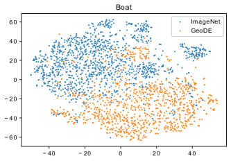
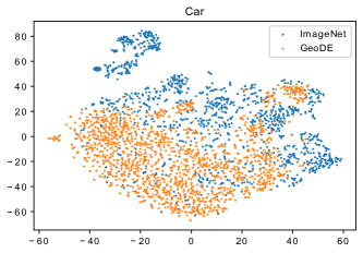
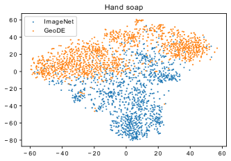
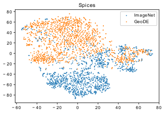
Figure 11: We visualize the TSNE plots for several of object classes using ImageNet and GeoDE . While the features do overlap slightly, on the whole, they are very different for dataset distributions, even within each category.

Appendix C More results using GeoDE as an evaluation dataset

Here, we provide more more analysis performed on using GeoDE as an evaluation dataset. As shown in sec. 5 of the main text, CLIP models perform worse on certain objects (e.g “house”, “spices”, “medicine”, etc.). Visualizing the probabilities assigned to different images from the same class as a box plot, we see different scenarios emerge: the variance of scores is large for all regions, as in the case of spices; the variance is large for certain regions, as in the case of stoves from Africa and East and Southeast Asia, or the scores are much lower for a specific region, as in the case of religious buildings in East Asia (12).

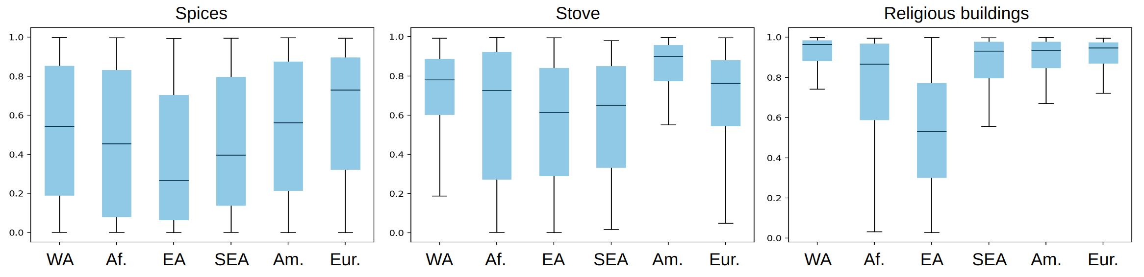
Figure 12: We visualize the probabilities assigned by CLIP to different images from the same class as a box plot. We see that the images across different regions have scores that vary in different ways: for “spices”, we see a large variance for all regions; for “stoves”, the variance is large for stoves from Africa, and Southeast and East Asia, but much smaller for other regions. For “religious buildings”, we see that the scores are just much lower for buildings in East Asia.

Appendix D More results when training with GeoDE

In this section, we provide results for the incremental training with GeoDE for different regions that were not presented in Sec 7, and provide results when fine-tuning a ResNet50 model, rather than freezing the layer weights.

D.1 Results from incrementally adding additional regions

We visualize the improvement in the accuracy as we incrementally add in images from different regions (Sec. 6.2 in the main text). We can see that the performance both within the specific region and in Europe (compared to Americas when considering Europe) increase with the additional GeoDE data. We see that the increase within the region is larger than that of the control, showing that these images are from different domains. (Fig. 13)

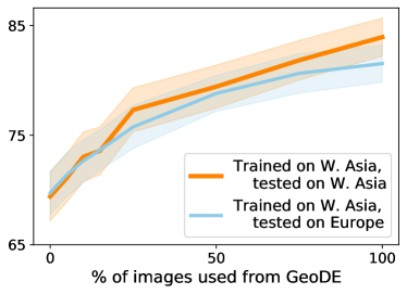
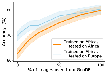
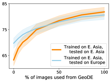
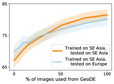
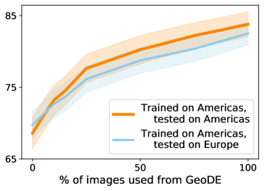
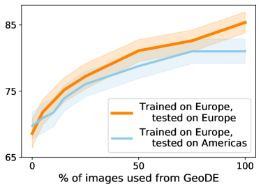
Figure 13: We visualize the increase in accuracy as images are incrementally added in from a region. We find that while adding any GeoDE regional images increases the performance of the model on European images, it has a larger effect on the region the images were drawn from.

D.2 Results from finetuning a ResNet50 model

Implementation details. We use a ResNet50 [15] model pretrained on Imagenet and fine tune the weights using different fractions of the ImageNet and GeoDE datasets as mentioned in Sec. 7 in the main paper. We train the model with an SGD optimizer, learning rate = 0.1, and momentum=0.9. Other implementation details remain the same as before.

Results. While the overall trend of the results are the same, we see that these results are slightly noisier, potentially because the model overfits to the small training set (Fig. 14).

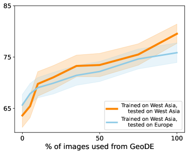
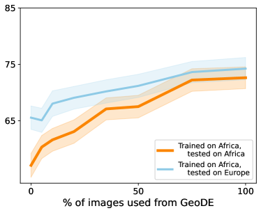
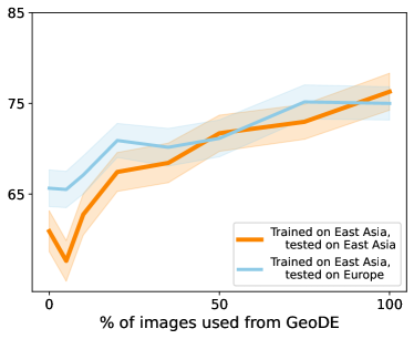
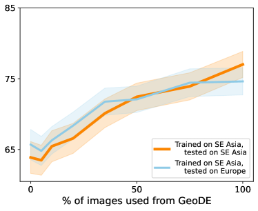
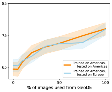
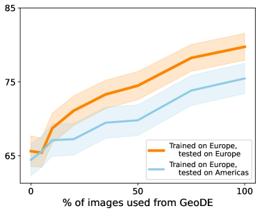
Figure 14: We visualize the increase in accuracy as images are incrementally added in from a region when finetuning a ResNet50 model. Similar to Fig. 10 in the main text, we see that adding in GeoDE images increases performance more in the region than a control.

Appendix E More details about the dataset

In this supplementary section, we provide counts of the objects per region in GeoDE as well as more examples of images from this dataset. .

As mentioned before, GeoDE is mostly balanced across both region and object: for most part, we were able to get atleast 150 images per region per object, with a few exceptions (“wheelbarrow” in 2 regions; “monument”, “boat” and “flag” in 1 region). See Tab. 10 for full counts.

	West Asia	Africa	East Asia	Southeast Asia	Americas	Europe
backyard	216	670	192	218	217	226
bag	267	397	370	593	298	437
bicycle	237	257	298	235	228	241
boat	162	227	174	237	84	222
bus	203	240	223	214	217	226
candle	232	244	220	239	188	270
car	242	331	276	235	273	363
chair	279	365	326	512	344	349
cleaning equipment	259	284	307	305	270	361
cooking pot	216	270	228	202	213	304
dog	219	194	185	244	206	193
dustbin	220	423	266	203	271	294
fence	259	322	244	302	226	282
flag	206	265	139	223	206	272
front_door	210	254	216	224	200	235
hairbrush/comb	269	255	307	300	290	431
hand soap	222	208	277	191	245	362
hat	209	297	337	316	294	336
house	199	437	208	195	277	194
jug	217	211	186	249	236	194
light fixture	234	344	248	209	191	300
light switch	215	240	246	273	273	234
lighter	221	312	225	237	217	268
medicine	242	286	310	330	328	300
monument	161	191	186	183	254	245
plate of food	211	480	294	364	241	304
religious building	222	230	204	226	197	229
road sign	226	416	258	270	235	284
spices	243	250	331	216	290	300
stall	143	215	203	227	197	221
storefront	209	306	191	240	243	204
stove	199	553	191	262	206	282
streetlight / lantern	202	346	211	196	208	227
toothbrush	264	258	330	361	337	270
toothpaste / toothpowder	209	288	269	230	245	315
toy	224	221	280	292	323	287
tree	226	308	245	357	300	328
truck	205	246	207	231	212	225
waste container	231	213	209	213	211	253
wheelbarrow	122	267	130	197	152	243

Table 10: We show the counts of objects per region in GeoDE. Bolded are the ones categories for which we were not able to get 175 images per region.

We also provide more examples of the images from GeoDE in the Figures Figs. 15, 16, 17, 18, 19, 20, 21, 22, 23, 24, 25, 26, 27 and 28.

Backyard
West Asia
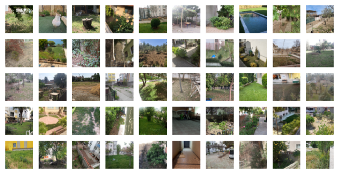
Africa
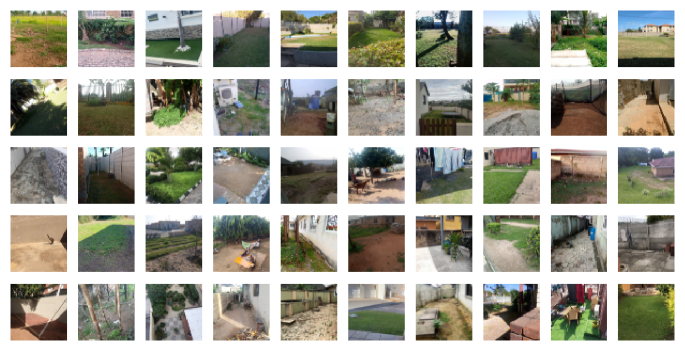
East Asia

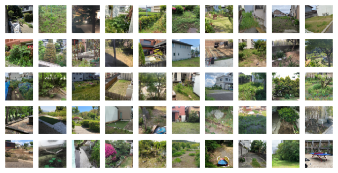
Figure 15: Randomly chosen images for “backyard” for 3 regions. We notice that some of these are backyards made of concrete (West Asia: r2c1, r3c4, etc., Africa: r3c1 ,r4c9, r5c3, etc.,) or do not contain lawns (West Asia: r3c1, r2c5, etc., Africa:r5c1-5, etc., East Asia: r2c4, r5c1, r5c4-6, etc.)

Backyard
Southeast Asia
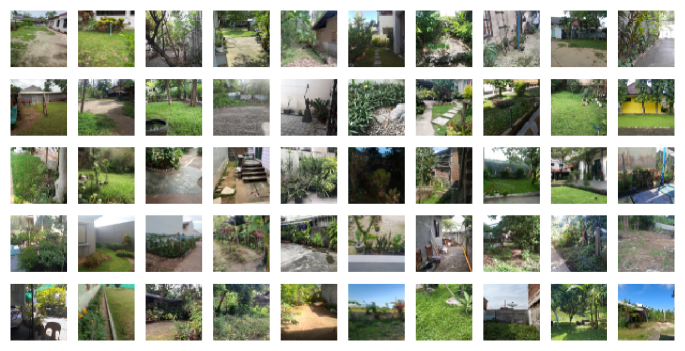
Americas
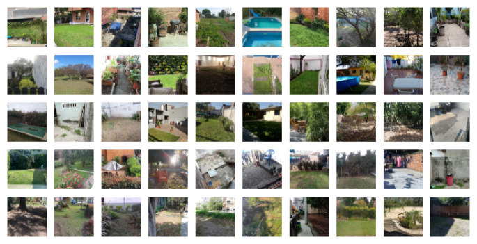
Europe

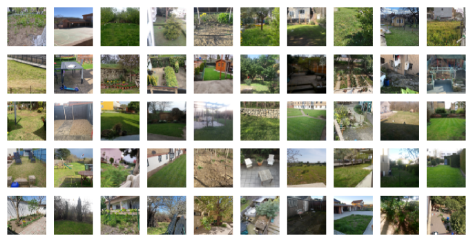
Figure 16: Randomly chosen images for “backyard” for the 3 other regions. Again, we see that regions tend to have backyards made of concrete or paved (Southeast Asia: r1c8, r2c5, r3c3 as examples, Americas: r1c9, r1c10, r2c10, etc., Europe: r3c2, r4c5, etc ), or do not contain lawns (Southeast Asia: r1c1, r1c9, etc., Americas:r3c2, r3c3, etc., Europe: r3c2, r5c9, etc.)

Bicycle
West Asia
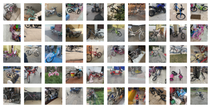
Africa
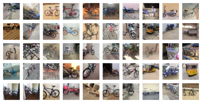
East Asia

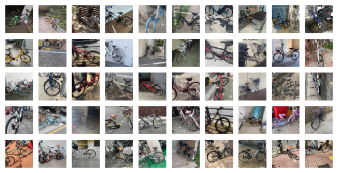
Figure 17: Randomly chosen images for “bicycle” for 3 regions. While most images are of standard bicycles, we notice a couple of interesting images: tricycle (West Asia: r4c9), rickshaws (Africa: r2c8, r2c10, r4c8, r4c10), and motorized cycles (West Asia: r1c8). There are also a lot of children’s bicycles.

Bicycle
Southeast Asia
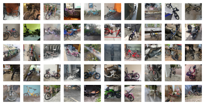
Americas
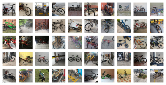
Europe

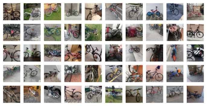
Figure 18: Randomly chosen images for “bicycle” for the 3 other regions. We see more motorized cycles (Southeast Asia: r5c6) as well as several children’s bicycles.

Boat
West Asia
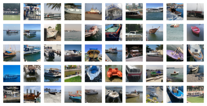
Africa
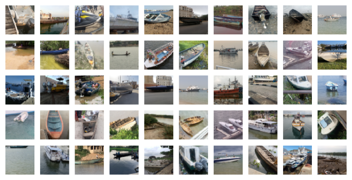
East Asia

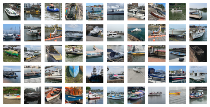
Figure 19: Randomly chosen images for “boat” for 3 regions. We see a variety of boats including larger ships in West Asia (r1c1, r1c2, r1c5, r4c1,r5c1), smaller kayaks and canoes in Africa (r1c8-9, r2c1-4, r4c2 , etc ), and a mix in East Asia.

Boat
Southeast Asia
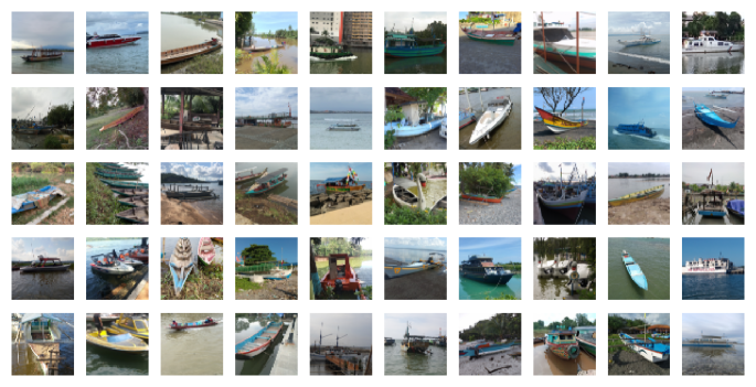
Americas
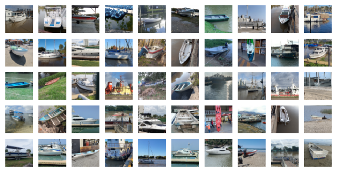
Europe

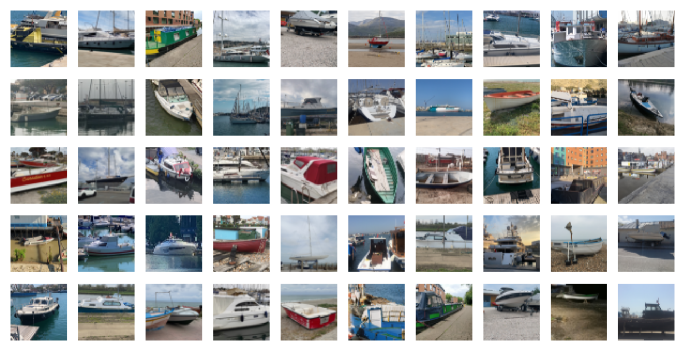
Figure 20: Randomly chosen images for “boat” for the 3 other regions. We again see a variety of boats ranging from motor boats in Europe and the Americas to smaller boats in Southeast Asia.

Cleaning equipment
West Asia
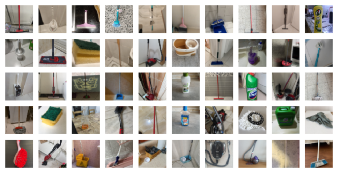
Africa
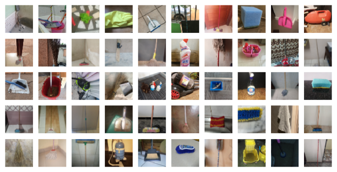
East Asia

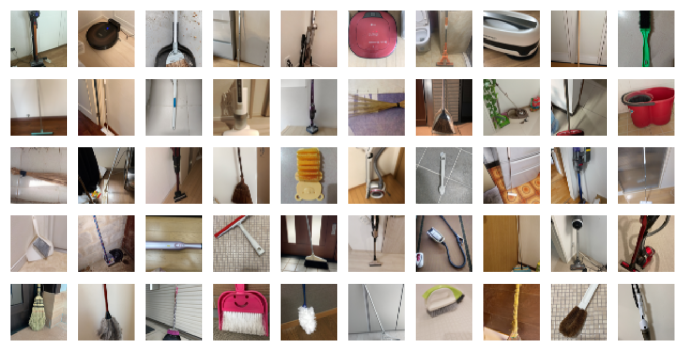
Figure 21: Randomly chosen images for “cleaning equipment” for 3 regions. This appears to be a diverse category within all regions containing images of mops, buckets, products, brooms, etc.

Cleaning equipment
Southeast Asia
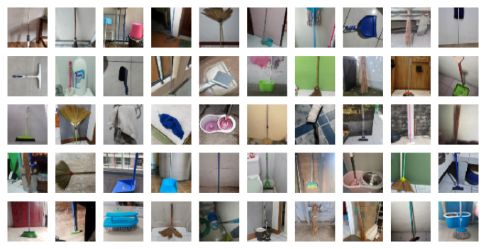
Americas
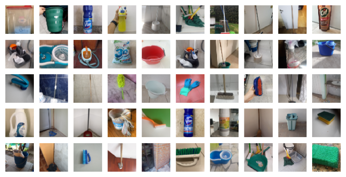
Europe

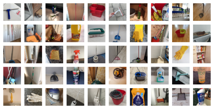
Figure 22: Randomly chosen images for “cleaning equipment” for the 3 other regions. This appears to be a diverse category within all regions containing images of mops, buckets, products, brooms, etc.

Spices
West Asia
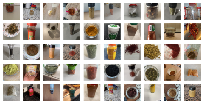
Africa
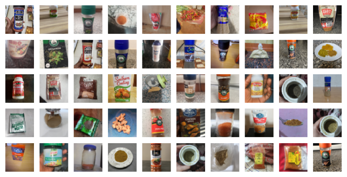
East Asia

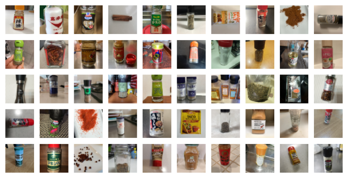
Figure 23: Randomly chosen images for “spices” for 3 regions. We see a wide range of containers, ranging from packets (mostly in Africa), glass jars (in West Asia) to some bottles (all regions).

Spices
Southeast Asia
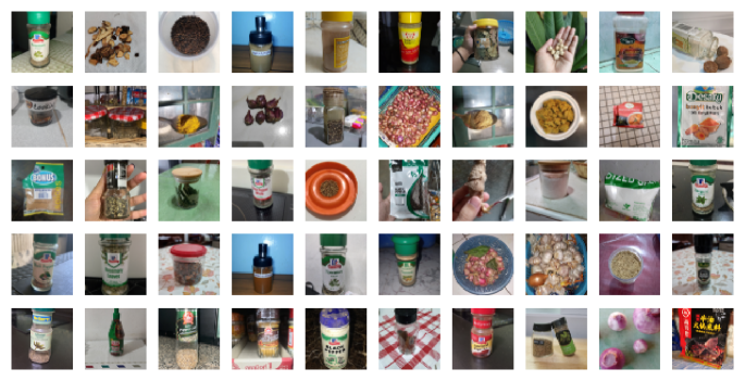
Americas
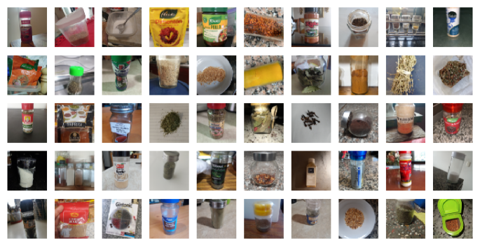
Europe

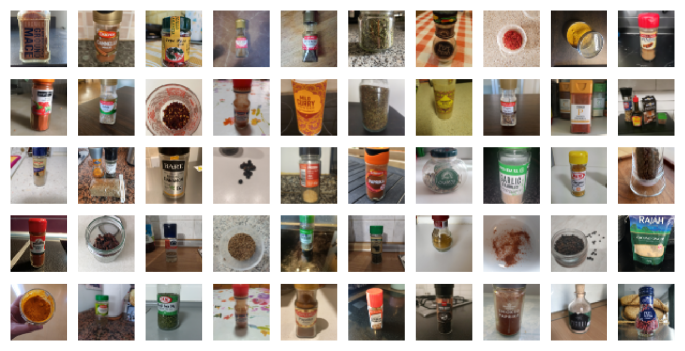
Figure 24: Randomly chosen images for “spices” for 3 regions. We see a wide range of containers, ranging from packets (some in Southeast Asia and Americas) to bottles (some in Southeast Asia)

Stove
West Asia
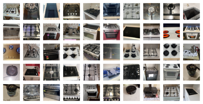
Africa
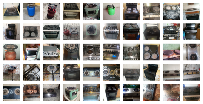
East Asia

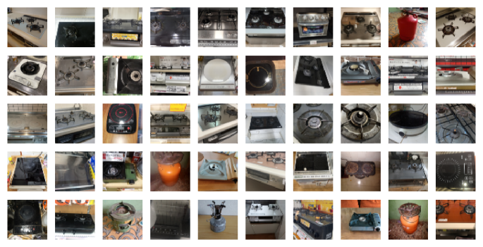
Figure 25: Randomly chosen images for “stove” for 3 regions. We see that Africa and East Asia contain one-burner and two burner stoves (along with 4 burner stoves). We also see a variety of stoves in terms of induction, gas, ovens, etc.

Stove
Southeast Asia
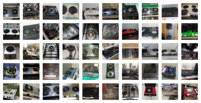
Americas
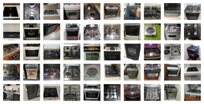
Europe

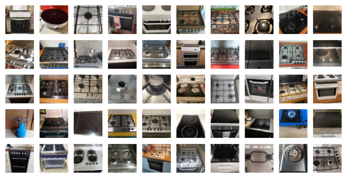
Figure 26: Randomly chosen images for “stove” for 3 regions. We see that Southeast Asia contains one-burner and two burner stoves (along with 4 burner stoves). We also see a variety of stoves in terms of induction, coils, gas, ovens, etc.

Waste container
West Asia
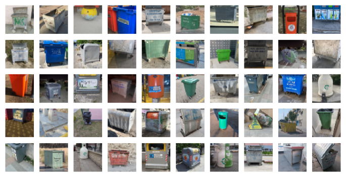
Africa
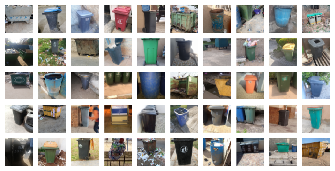
East Asia

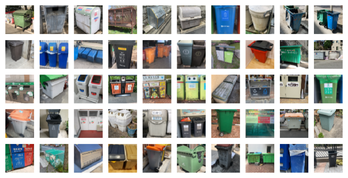
Figure 27: Randomly chosen images for “waste container” for 3 regions. We see that different regions have containers of varying sizes (Africa seems to be smaller than West Asia or East Asia), and have different closing mechanisms (see West Asia r5c6 as an interesting example.) East Asia also tends to have segregated waste containers.

Waste containers
Southeast Asia
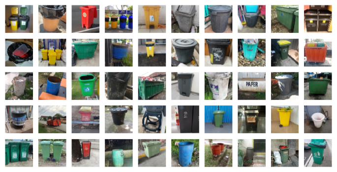
Americas
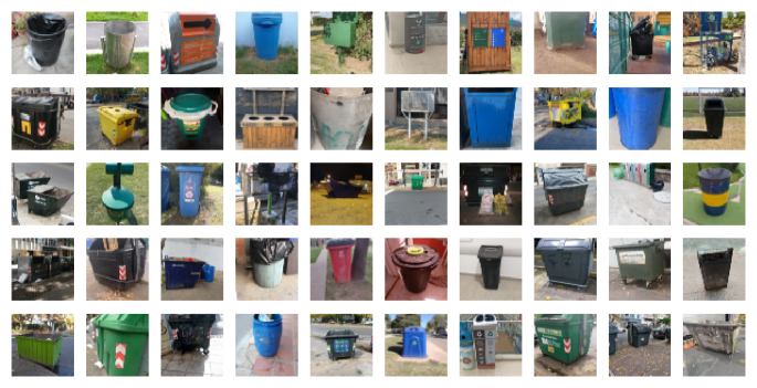
Europe

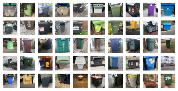
Figure 28: Randomly chosen images for “waste container” for 3 regions. We see that different regions have containers of varying sizes (Europe seems to have containers of very different sizes) and have different closing mechanisms (see Southeast Asia r2c6 as an interesting example.)

References

- [1] Open images extended. https://research.google/tools/datasets/open-images-extended-crowdsourced/. Accessed: 2022-10-16.
- [2] Yuki M. Asano, Christian Rupprecht, Andrew Zisserman, and Andrea Vedaldi. Pass: An imagenet replacement for self-supervised pretraining without humans. NeurIPS Track on Datasets and Benchmarks, 2021.
- [3] Abeba Birhane and Vinay Uday Prabhu. Large image datasets: A pyrrhic win for computer vision? In WACV, 2021.
- [4] Joy Buolamwini and Timnit Gebru. Gender shades: Intersectional accuracy disparities in commercial gender classification. In FAT, 2018.
- [5] Mathilde Caron, Ishan Misra, Julien Mairal, Priya Goyal, Piotr Bojanowski, and Armand Joulin. Unsupervised learning of visual features by contrasting cluster assignments. NeurIPS, 2020.
- [6] Dima Damen, Hazel Doughty, Giovanni Maria Farinella, Sanja Fidler, Antonino Furnari, Evangelos Kazakos, Davide Moltisanti, Jonathan Munro, Toby Perrett, Will Price, et al. Scaling egocentric vision: The epic-kitchens dataset. In ECCV, 2018.
- [7] Terrance De Vries, Ishan Misra, Changhan Wang, and Laurens Van der Maaten. Does object recognition work for everyone? In CVPR Workshops, 2019.
- [8] J. Deng, W. Dong, R. Socher, L.-J. Li, K. Li, and L. Fei-Fei. ImageNet: A Large-Scale Hierarchical Image Database. In CVPR, 2009.
- [9] Abhimanyu Dubey, Vignesh Ramanathan, Alex Pentland, and Dhruv Mahajan. Adaptive methods for real-world domain generalization. In CVPR, 2021.
- [10] Chris Dulhanty and Alexander Wong. Auditing ImageNet: Towards a model-driven framework for annotating demographic attributes of large-scale image datasets. arXiv preprint arXiv:1905.01347, 2019.
- [11] M. Everingham, L. Van Gool, C. K. I. Williams, J. Winn, and A. Zisserman. The pascal visual object classes (voc) challenge. IJCV, 2010.
- [12] Li Fei-Fei, R. Fergus, and P. Perona. Learning generative visual models from few training examples: An incremental bayesian approach tested on 101 object categories. In CVPR, 2004.
- [13] Kristen Grauman, Andrew Westbury, Eugene Byrne, Zachary Chavis, Antonino Furnari, Rohit Girdhar, Jackson Hamburger, Hao Jiang, Miao Liu, Xingyu Liu, Miguel Martin, Tushar Nagarajan, Ilija Radosavovic, Santhosh Kumar Ramakrishnan, Fiona Ryan, Jayant Sharma, Michael Wray, Mengmeng Xu, Eric Zhongcong Xu, Chen Zhao, Siddhant Bansal, Dhruv Batra, Vincent Cartillier, Sean Crane, Tien Do, Morrie Doulaty, Akshay Erapalli, Christoph Feichtenhofer, Adriano Fragomeni, Qichen Fu, Christian Fuegen, Abrham Gebreselasie, Cristina González, James Hillis, Xuhua Huang, Yifei Huang, Wenqi Jia, Weslie Khoo, Jáchym Kolár, Satwik Kottur, Anurag Kumar, Federico Landini, Chao Li, Yanghao Li, Zhenqiang Li, Karttikeya Mangalam, Raghava Modhugu, Jonathan Munro, Tullie Murrell, Takumi Nishiyasu, Will Price, Paola Ruiz Puentes, Merey Ramazanova, Leda Sari, Kiran Somasundaram, Audrey Southerland, Yusuke Sugano, Ruijie Tao, Minh Vo, Yuchen Wang, Xindi Wu, Takuma Yagi, Yunyi Zhu, Pablo Arbelaez, David Crandall, Dima Damen, Giovanni Maria Farinella, Bernard Ghanem, Vamsi Krishna Ithapu, C. V. Jawahar, Hanbyul Joo, Kris Kitani, Haizhou Li, Richard A. Newcombe, Aude Oliva, Hyun Soo Park, James M. Rehg, Yoichi Sato, Jianbo Shi, Mike Zheng Shou, Antonio Torralba, Lorenzo Torresani, Mingfei Yan, and Jitendra Malik. Ego4d: Around the world in 3, 000 hours of egocentric video. arXiv, 2021.
- [14] Gregory Griffin, Alex Holub, and Pietro Perona. Caltech-256 object category dataset. 2007.
- [15] Kaiming He, Xiangyu Zhang, Shaoqing Ren, and Jian Sun. Deep residual learning for image recognition. In CVPR, 2016.
- [16] Kaiming He, Xiangyu Zhang, Shaoqing Ren, and Jian Sun. Identity mappings in deep residual networks. In ECCV, 2016.
- [17] Alina Kuznetsova, Hassan Rom, Neil Alldrin, Jasper Uijlings, Ivan Krasin, Jordi Pont-Tuset, Shahab Kamali, Stefan Popov, Matteo Malloci, Alexander Kolesnikov, Tom Duerig, and Vittorio Ferrari. The open images dataset v4: Unified image classification, object detection, and visual relationship detection at scale. IJCV, 2020.
- [18] George A Miller. Wordnet: a lexical database for english. Comm. ACM, 1995.
- [19] F. Pedregosa, G. Varoquaux, A. Gramfort, V. Michel, B. Thirion, O. Grisel, M. Blondel, P. Prettenhofer, R. Weiss, V. Dubourg, J. Vanderplas, A. Passos, D. Cournapeau, M. Brucher, M. Perrot, and E. Duchesnay. Scikit-learn: Machine learning in Python. JMLR, 2011.
- [20] Alec Radford, Jong Wook Kim, Chris Hallacy, Aditya Ramesh, Gabriel Goh, Sandhini Agarwal, Girish Sastry, Amanda Askell, Pamela Mishkin, Jack Clark, Gretchen Krueger, and Ilya Sutskever. Learning transferable visual models from natural language supervision. In ICML, 2021.
- [21] William A Gaviria Rojas, Sudnya Diamos, Keertan Ranjan Kini, David Kanter, Vijay Janapa Reddi, and Cody Coleman. The dollar street dataset: Images representing the geographic and socioeconomic diversity of the world. In NeurIPS Datasets&Benchmarks Track, 2022.
- [22] Olga Russakovsky, Jia Deng, Hao Su, Jonathan Krause, Sanjeev Satheesh, Sean Ma, Zhiheng Huang, Andrej Karpathy, Aditya Khosla, Michael Bernstein, Alexander C. Berg, and Li Fei-Fei. Imagenet large scale visual recognition challenge. IJCV, 2015.
- [23] Shreya Shankar, Yoni Halpern, Eric Breck, James Atwood, Jimbo Wilson, and D Sculley. No classification without representation: Assessing geodiversity issues in open data sets for the developing world. NeurIPS Workshop on Machine Learning for the Developing World , 2017.
- [24] Gunnar A. Sigurdsson, Gül Varol, X. Wang, Ali Farhadi, Ivan Laptev, and Abhinav Kumar Gupta. Hollywood in homes: Crowdsourcing data collection for activity understanding. ECCV, 2016.
- [25] Pierre Stock and Moustapha Cisse. Convnets and imagenet beyond accuracy: Understanding mistakes and uncovering biases. In ECCV, 2018.
- [26] Bart Thomee, David A. Shamma, Gerald Friedland, Benjamin Elizalde, Karl Ni, Douglas Poland, Damian Borth, and Li-Jia Li. Yfcc100m: The new data in multimedia research. 2016.
- [27] Antonio Torralba and Alexei A Efros. Unbiased look at dataset bias. In CVPR, 2011.
- [28] Laurens van der Maaten and Geoffrey Hinton. Visualizing data using t-sne. JMLR, 2008.
- [29] Angelina Wang, Alexander Liu, Ryan Zhang, Anat Kleiman, Leslie Kim, Dora Zhao, Iroha Shirai, Arvind Narayanan, and Olga Russakovsky. REVISE: A tool for measuring and mitigating bias in visual datasets. IJCV, 2022.
- [30] Angelina Wang, Arvind Narayanan, and Olga Russakovsky. REVISE: A tool for measuring and mitigating bias in visual datasets. In ECCV, 2020.
- [31] Kaiyu Yang, Klint Qinami, Li Fei-Fei, Jia Deng, and Olga Russakovsky. Towards fairer datasets: Filtering and balancing the distribution of the people subtree in the imagenet hierarchy. In FAT, 2020.
- [32] Kaiyu Yang, Jacqueline Yau, Li Fei-Fei, Jia Deng, and Olga Russakovsky. A study of face obfuscation in imagenet. CoRR, abs/2103.06191, 2021.
- [33] Jieyu Zhao, Tianlu Wang, Mark Yatskar, Vicente Ordonez, and Kai-Wei Chang. Men also like shopping: Reducing gender bias amplification using corpus-level constraints. In EMNLP, 2017.