The Ulam-Hammersley problem for multiset permutations

Abstract

We obtain the asymptotic behaviour of the longest increasing/non-decreasing subsequences in a random uniform multiset permutation in which each element in $\{1,\dots,n\}$ occurs $k$ times, where $k$ may depend on $n$. This generalizes the famous Ulam-Hammersley problem of the case $k=1$. The proof relies on poissonization and a connection with variants of the Hammersley-Aldous-Diaconis particle system.

1 Introduction

A $k$-multiset permutation of size $n$ is a word with letters in $\{1,2,\dots,n\}$ such that each letter appears exactly $k$ times. When this is convenient we identify a multiset permutation $s=\left(s(1),\dots,s(kn)\right)$ and the set of points $\{(i,s(i)),\ 1\leq i\leq kn\}$. For example we say that there is a point at height $j$ in $s$ is $s(i)=j$ for some $i$.

We introduce two partial orders over the quarter-plane $[0,\infty)^{2}$:

$$(x,y)\prec(x^{\prime},y^{\prime}) \text{ if }x<x^{\prime}\text{ and }y<y^{\prime},$$

$$(x,y)\preccurlyeq(x^{\prime},y^{\prime}) \text{ if }x<x^{\prime}\text{ and }y\leq y^{\prime}.$$

(Note that the roles of $x,y$ are not identical in the definition of $\preccurlyeq$.) For a finite set $\mathcal{P}$ of points in the quarter-plane we put

$$\mathcal{L}_{<}(\mathcal{P}) =\max\left\{L;\hbox{ there exists }P_{1}\prec P_{2}\prec\dots\prec P_{L},\text{ where each }P_{i}\in\mathcal{P}\right\},$$

$$\mathcal{L}_{\leq}(\mathcal{P}) =\max\left\{L;\hbox{ there exists }P_{1}\preccurlyeq P_{2}\preccurlyeq\dots\preccurlyeq P_{L},\text{ where each }P_{i}\in\mathcal{P}\right\}.$$

The integer $\mathcal{L}_{<}(\mathcal{P})$ (resp. $\mathcal{L}_{\leq}(\mathcal{P})$) is the length of the longest increasing (resp. non-decreasing) subsequence of $\mathcal{P}$.

Let $S_{k;n}$ be a $k$-multiset permutation of size $n$ taken uniformly among the $\binom{kn}{k\ k\ \dots\ k}$ possibilities. In the case $k=1$ the word $S_{1;n}$ is just a uniform permutation and estimating $\mathcal{L}_{<}(S_{1;n})$ is known as the Hammersley or Ulam-Hammersley problem. The first order was solved by Veršik and Kerov [VK77] (see [Rom15] for a review of the problem):

$$\mathbb{E}[\mathcal{L}_{<}(S_{1;n})]=\mathbb{E}[\mathcal{L}_{\leq}(S_{1;n})]\stackrel{{\scriptstyle n\to+\infty}}{{\sim}}2\sqrt{n}.$$

Note that the above limit also holds in probability, in the sense that $\mathbb{P}\left(|\tfrac{1}{2\sqrt{n}}\mathcal{L}_{<}(S_{1;n})-1|>\varepsilon\right)\to 0$ for every $\varepsilon>0$, that we shorten into: $\mathcal{L}_{<}(S_{1;n})=2\sqrt{n}+\mathrm{o}_{\mathbb{P}}(\sqrt{n})$.

In the context of card guessing games it is asked in [CDH⁺22, Question 4.3] the behaviour of $\mathcal{L}_{<}(S_{k;n})$ for a fixed $k$. Using known results regarding longest increasing subsequences through independent points we can make an educated guess. Indeed, let $\mathrm{Ber}^{(p)}$ be a field of i.i.d. Bernoulli random variables with mean $p$ over the square lattice. Seppäläinen [Sep97, Th.1.] proved that for fixed $p$ and $k$,

$$\mathcal{L}_{<}\left(\mathrm{Ber}^{(p)}\cap[0,kn]\times[0,n]\right)\stackrel{{\scriptstyle n\to\infty}}{{\sim}}n\times\frac{\sqrt{p}}{1-p}\left(2\sqrt{k}-(k+1)\sqrt{p}\right).$$

For $p=1/n$ there are in average $k$ points of $\mathrm{Ber}^{(p)}$ on each line of $[0,kn]\times[0,n]$. Pretending that we can safely let $p$ depend on $n$ in the above approximation we obtain

$$\mathcal{L}_{<}(S_{k;n})\approx\mathcal{L}_{<}\left(\mathrm{Ber}^{(1/n)}\cap[0,kn]\times[0,n]\right)\approx 2\sqrt{kn}.$$

The goal of the present paper is to make this approximation rigorous (however we are not going to use Seppäläinen’s result but rather poissonize the problem). We actually adress this question in the case where $k$ depends on $n$.

Theorem 1 (Longest increasing subsequences).

Let $(k_{n})$ be a sequence of integers such that $k_{n}\leq n$ for all $n$. Then

$$\mathbb{E}[\mathcal{L}_{<}(S_{k_{n};n})]=2\sqrt{nk_{n}}-k_{n}+o(\sqrt{nk_{n}}).$$ (1)

(Of course if $k_{n}=o(n)$ then the RHS of (1) reduces to $2\sqrt{nk_{n}}+\mathrm{o}(\sqrt{nk_{n}})$.) If $k_{n}\geq n$ for some $n$ then the naive greedy strategy shows very easily that $\mathbb{E}[\mathcal{L}_{<}(S_{k_{n};n})]\geq n-\mathrm{o}(n)$.

Theorem 2 (Longest non-decreasing subsequences).

Let $(k_{n})$ be an arbitrary sequence of integers. Then

$$\mathbb{E}[\mathcal{L}_{\leq}(S_{k_{n};n})]=2\sqrt{nk_{n}}+k_{n}+o(\sqrt{nk_{n}}).$$ (2)

We are not aware of previous results for multiset permutations. However Theorems 1 and 2 in the linear regime $k_{n}\sim\mathrm{constant}\times n$ should be compared to a result by Biane ([Bia01, Theorem 3]). Indeed he obtains the exact limiting shape of the random Young Tableau induced through the RSK correspondence by a random word $\mathcal{W}_{q;N}$ of $q$ i.i.d. uniform letters in $\{1,2,\dots,N\}$ in the regime where $\sqrt{q}/N\to c$ for some constant $c>0$. (The regime $\sqrt{q}/N\to c$ corresponds to $k_{n}\sim c^{2}n$ with our notation.) Regarding longest increasing subsequences we expect the asymptotics of the word $\mathcal{W}_{q;N}$ to be close to that of the multiset permutation $S_{c^{2}N;N}$ and Theorems 1 and 2 respectively suggest:

$$L_{<}(\mathcal{W}_{q;N})\approx L_{<}(S_{c^{2}N;N})\sim 2Nc-c^{2}N\sim(2-c)\sqrt{q},$$

$$L_{\leq}(\mathcal{W}_{q;N})\approx L_{\leq}(S_{c^{2}N;N})\sim 2Nc+c^{2}N\sim(2+c)\sqrt{q}.$$

As the length of the first row (resp. the number of rows) in the Young Tableau corresponds to the length of the longest non-decreasing subsequence in $\mathcal{W}_{k;n}$ (resp. the length of the longest decreasing sequence) a weak consequence of ([Bia01, Theorem 3]) is that, in probability,

$$\liminf\frac{1}{\sqrt{q}}L_{<}(\mathcal{W}_{q;N})\geq(2-c),\qquad\limsup\frac{1}{\sqrt{q}}L_{\leq}(\mathcal{W}_{q;N})\leq(2+c),$$

which is indeed consistent with the above heuristic.

Strategy of proof and organization of the paper.

In Section 2 we first provide the proof of Theorems 1 and 2 in the case of a constant or slowly growing sequence $(k_{n})$. The proof is elementary (assuming known the Veršik-Kerov Theorem).

For the general case we first borrow a few tools in the literature. In particular we introduce and analyze poissonized versions of $\mathcal{L}_{<}(S_{k_{n};n}),\mathcal{L}_{\leq}(S_{k_{n};n})$. As already suggested by Hammersley ([Ham72], Sec.9) and achieved by Aldous-Diaconis [AD95] the case $k=1$ can be tackled by considering an interacting particle system which is now known as the Hammersley or Hammersley-Aldous-Diaconis (HAD) process.

In Section 3 we introduce and analyze the two variants of the Hammersley process adapted to multiset permutations.. The first one is the discrete-time HAD process [Fer96, FM06], the second one had recently appeared in [Boy22] with a connection to the O’Connell-Yor Brownian polymer. The standard path to analyze Hammersley-like processes consists in using subadditivity to prove the existence of a limiting shape and then proving that this limiting shape satisfies a variational problem. Typically this variational problem is solved either using convex duality [Sep97, CG19] or through the analysis of second class particles [CG06, CG19]. The issue here is that since we allow $k_{n}$ to have different scales we cannot use this approach and we need to derive non-asymptotic bounds for both processes. This is the purpose of Theorem 9 whose proof is the most technical part of the paper. In Section 4 we detail the multivariate de-poissonization procedure in order to conclude the proof of Theorem 1. De-poissonization is more convoluted for non-decreasing subsequences: see Section 5.

Beyond expectation.

In the course of the proof we actually obtain results beyond the estimation of the expectation. We obtain concentration inequalities for the poissonized version of $\mathcal{L}_{<}(S_{k_{n};n}),\mathcal{L}_{\leq}(S_{k_{n};n})$: see Theorem 9 and also the discussion in Section 5.3. We also obtain the convergence in probability for most regimes of $(k_{n})$.

Proposition 3.

Let $(k_{n})$ be either a small or a large sequence. (See (4),(29) for the definitions of small/large sequences.) Then

$$\frac{\mathcal{L}_{<}(S_{k_{n};n})}{2\sqrt{nk_{n}}-k_{n}}\stackrel{{\scriptstyle\text{prob.}}}{{\to}}1,\qquad\frac{\mathcal{L}_{\leq}(S_{k_{n};n})}{2\sqrt{nk_{n}}+k_{n}}\stackrel{{\scriptstyle\text{prob.}}}{{\to}}1.$$ (3)

Regarding fluctuations a famous result by Baik, Deift and Johansson [BDJ99, Th.1.1] states that

$$\frac{\mathcal{L}_{\leq}(S_{1;n})-2\sqrt{n}}{n^{1/6}}\stackrel{{\scriptstyle(d)}}{{\to}}\mathrm{TW}$$

where $\mathrm{TW}$ is the Tracy-Widom distribution. The intuition given by the comparison with the Hammersley process would suggest that the fluctuations of $\mathcal{L}_{<}(S_{k_{n};n})$, $\mathcal{L}_{\leq}(S_{k_{n};n})$ might be of order $(k_{n}n)^{1/6}$ as long as $(k_{n})$ does not grow too fast. Yet we have no evidence for this.

2 Preliminaries: the case of small $k_{n}$

We first prove Theorems 1 and 2 in the case of a small sequence $(k_{n})$. We say that a sequence $(k_{n})$ of integers is small if

$$k_{n}^{2}(k_{n})!=\mathrm{o}(\sqrt{n}).$$ (4)

Note that a sequence of the form $k_{n}=(\log n)^{1-\varepsilon}$ is small while $k_{n}=\log n$ is not small.

Proof of Theorems 1 and 2 in the case of a small sequence $(k_{n})$.

(In order to lighten notation we skip the dependence in $n$ and write $k=k_{n}$.)
Let $\sigma_{kn}$ be a random uniform permutation of size $kn$. We can associate to $\sigma_{kn}$ a $k$-multiset permutation $S_{k;n}$ in the following way. For every $1\leq i\leq kn$ we put

$$S_{k;n}(i)=\lceil\sigma(i)/k\rceil.$$

It is clear that $S_{k;n}$ is uniform and we have

$$\mathcal{L}_{<}(S_{k;n})\leq\mathcal{L}_{\leq}(\sigma_{kn})\leq\mathcal{L}_{\leq}(S_{k;n}).$$

The Veršik-Kerov Theorem says that the middle term in the above inequality grows like $2\sqrt{kn}$. Hence we need to show that if $(k_{n})$ is small then

$$\mathcal{L}_{\leq}(S_{k;n})=\mathcal{L}_{<}(S_{k;n})+o_{\mathbb{P}}(\sqrt{kn}),$$

which proves the small case of Proposition 3 and Theorems 1 and 2. For this purpose we introduce for every $\delta>0$ the event

$$\mathcal{E}_{\delta}:=\left\{\mathcal{L}_{\leq}(S_{k;n})\geq\mathcal{L}_{<}(S_{k;n})+\delta\sqrt{n}\right\}.$$ (5)

If $\mathcal{E}_{\delta}$ occurs then in particular there exists a non-decreasing subsequence with $\delta\sqrt{n}$ ties, i.e. points of $S_{k;n}$ which are at the same height as their predecessor in the subsequence. These ties have distinct heights $1\leq i_{1}<\dots<i_{\ell}\leq n$ for some $\delta\sqrt{n}/k\leq\ell\leq\delta\sqrt{n}$. Fix

• Integers $m_{1},\dots,m_{\ell}\geq 2$ such that $(m_{1}-1)+\dots+(m_{\ell}-1)=\delta\sqrt{n}$ ;

• Column indices $r_{1,1}<\dots<r_{1,m_{1}}<r_{2,1}<r_{2,m_{1}}<\dots<r_{\ell,1}<\dots<r_{1,m_{\ell}}$.

We then introduce the event

$$F=F\left((i_{\ell})_{\ell},(r_{i,j})_{i\leq\ell,j\leq m_{i}}\right)\\ =\left\{S(r_{1,1})=\dots=S(r_{1,m_{1}})=i_{1},S(r_{2,1})=\dots=S(r_{2,m_{1}})=i_{2},\dots,S(r_{\ell,1})=\dots=S(r_{1,m_{\ell}})=i_{\ell}\right\}.$$

By the union bound (we skip the integer parts)

$$\mathbb{P}(\mathcal{E}_{\delta})\leq\sum_{\delta\sqrt{n}/k\leq\ell\leq\delta\sqrt{n}}\ \ \sum_{1\leq i_{1}<\dots\leq i_{\ell}\leq n}\ \ \sum_{(r_{i,j})_{i\leq\ell,j\leq m_{i}}}\mathbb{P}\left(F\left((i_{\ell})_{\ell},(r_{i,j})_{i\leq\ell,j\leq m_{i}}\right)\right).$$

Using

$$\mathrm{card}\left\{\sum m_{i}=\delta\sqrt{n}+\ell;\text{ each }m_{i}\geq 2\right\}=\mathrm{card}\left\{\sum p_{i}=\delta\sqrt{n};\text{ each }p_{i}\geq 1\right\}=\binom{\delta\sqrt{n}-1}{\ell-1}$$

we obtain the upper bound

$$\sum_{(r_{i,j})_{i\leq\ell,j\leq m_{i}}}\mathbb{P}(F) =\frac{1}{\binom{kn}{k\ k\ \dots\ k}}\underbrace{\binom{nk}{\sum m_{i}}}_{\text{choices of $r$'s}}\ \underbrace{\binom{\delta\sqrt{n}-1}{\ell-1}}_{\text{choices of }m_{i}^{\prime}s}\ \underbrace{\binom{kn-\sum m_{i}}{(k-m_{1})\ (k-m_{2})\ \dots(k-m_{\ell})k\dots k}}_{\text{choices of $kn-\sum m_{i}$ remaining points}}$$

$$=\frac{(k!)^{\ell}(\delta\sqrt{n}-1)!}{(\delta\sqrt{n}+\ell)!(\delta\sqrt{n}-\ell)!(\ell-1)!(k-m_{1})!(k-m_{2})!\times\dots\times(k-m_{\ell})!}$$

$$\leq\frac{(k!)^{\ell}}{(\delta\sqrt{n})^{\ell+1}(\delta\sqrt{n}-\ell)!(\ell-1)!}.$$

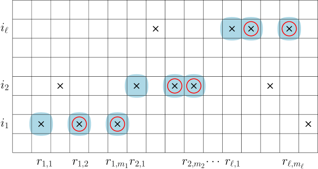
Figure 1: The event $F$. (Ties are surrounded in red. Points with blue background represent the subsequence with $\delta\sqrt{n}$ ties.)

We now sum over $1\leq i_{1}<\dots\leq i_{\ell}\leq n$ and then sum over $\ell$:

$$\mathbb{P}(\mathcal{E}_{\delta}) \leq\sum_{\ell=\delta\sqrt{n}/k}^{\delta\sqrt{n}}\binom{n}{\ell}\frac{(k!)^{\ell}}{(\delta\sqrt{n})^{\ell+1}(\delta\sqrt{n}-\ell)!(\ell-1)!}$$

$$\leq\sum_{\ell=\delta\sqrt{n}/k}^{\delta\sqrt{n}-3}\binom{n}{\ell}\frac{(k!)^{\ell}}{(\delta\sqrt{n})^{\ell+1}(\delta\sqrt{n}-\ell)!(\ell-1)!}+3\binom{n}{\delta\sqrt{n}}\frac{(k!)^{\delta\sqrt{n}}}{(\delta\sqrt{n})^{\delta\sqrt{n}-2}(\delta\sqrt{n}-3)!}$$ (6)

Using the two following inequalities valid for every $j\leq m$ (see e.g. [CLRS09, eq.(C.5)])

$$\binom{m}{j}\leq\left(\frac{me}{j}\right)^{j},\qquad m!\geq m^{m}\exp(-m)$$

we first obtain that if $k_{n}!=\mathrm{o}(\sqrt{n})$ (which is the case if $(k_{n})$ is small) then the last term of (6) tends to zero. Regarding the sum we write

$$\mathbb{P}(\mathcal{E}_{\delta}) \leq\sum_{\ell=\delta\sqrt{n}/k}^{\delta\sqrt{n}-3}\left(\frac{ne}{\ell}\right)^{\ell}\frac{(k!)^{\ell}}{(\delta\sqrt{n})^{\ell+1}(\delta\sqrt{n}-\ell)^{\delta\sqrt{n}-\ell}e^{-\delta\sqrt{n}+\ell}(\ell-1)^{\ell-1}e^{-\ell+1}}+\mathrm{o}(1)$$

$$\leq\sum_{\ell=\delta\sqrt{n}/k}^{\delta\sqrt{n}-3}\left(\frac{nek!(\delta\sqrt{n}-\ell)}{\delta\sqrt{n}\ell(\ell-1)}\right)^{\ell}\frac{(\ell-1)e^{-1}}{\delta\sqrt{n}}\big{(}\underbrace{\frac{e}{\delta\sqrt{n}-\ell}}_{\leq e/3<1}\big{)}^{\delta\sqrt{n}}+\mathrm{o}(1)$$

$$\leq\sum_{\ell=\delta\sqrt{n}/k}^{\delta\sqrt{n}-3}\left(\frac{\sqrt{n}ek!(\delta\sqrt{n}-\ell)}{\delta\ell(\ell-1)}\right)^{\ell}\frac{(\ell-1)e^{-1}}{\delta\sqrt{n}}\big{(}\frac{e}{\delta\sqrt{n}-\ell}\big{)}^{\ell}+\mathrm{o}(1)$$

$$\leq\sum_{\ell=\delta\sqrt{n}/k}^{\delta\sqrt{n}-3}\left(\frac{\sqrt{n}e^{2}k!}{\delta\ell(\ell-1)}\right)^{\ell}\frac{(\ell-1)e^{-1}}{\delta\sqrt{n}}+\mathrm{o}(1),$$ (7)

which tends to zero for every $\delta>0$, as long as $(k_{n})$ satisfies (4). This proves that $\mathcal{L}_{\leq}(S_{k;n})=\mathcal{L}_{<}(S_{k;n})+o_{\mathbb{P}}(\sqrt{kn})$. Using the crude bounds $\mathcal{L}_{<}(S_{k;n})\leq n$ and $\mathcal{L}_{\leq}(S_{k;n})\leq kn$, eq.(7) also implies that

$$\mathbb{E}[\mathcal{L}_{\leq}(S_{k;n})]=\mathbb{E}[\mathcal{L}_{<}(S_{k;n})]+o(\sqrt{kn}),$$

which proves the small cases of Theorems 1 and 2 and Proposition 3.∎

3 Poissonization: variants of the Hammersley process

Remark.

In the sequel, $\mathrm{Poisson}(\mu)$ (resp. $\mathrm{Binomial}(n,q)$) stand for generic random variables with Poisson distribution with mean $\mu$ (resp. Binomial distribution with parameters $n,q$).
Notation $\mathrm{Geometric}_{\geq 0}(1-\beta)$ stands for a geometric random variable with the convention $\mathbb{P}(\mathrm{Geometric}_{\geq 0}(1-\beta)=k)=(1-\beta)\beta^{k}$ for $k\geq 0$. In particular $\mathbb{E}[\mathrm{Geometric}_{\geq 0}(1-\beta)]=\frac{\beta}{1-\beta}$.

3.1 Definitions of the processes $L_{<}(t)$ and $L_{\leq}(t)$

In this Section we define formally and analyze two semi-discrete variants of the Hammersley process.

For a parameter $\lambda>0$ let $\Pi^{(\lambda)}$ be the random set $\Pi^{(\lambda)}=\cup_{i}\Pi_{i}^{(\lambda)}$ where $\Pi^{(\lambda)}_{i}$’s are independent and each $\Pi^{(\lambda)}_{i}$ is a homogeneous Poisson Point Process (PPP) with intensity $\lambda$ on $(0,\infty)\times\{i\}$. For simplicity set

$$\Pi^{(\lambda)}_{x,t}=\Pi^{(\lambda)}\cap\left([0,x]\times\{1,\dots,t\}\right).$$

The goal of the present section is to obtain non-asymptotic bounds for $\mathcal{L}_{<}\left(\Pi^{(\lambda)}_{x,t}\right)$ and $\mathcal{L}_{\leq}\left(\Pi^{(\lambda)}_{x,t}\right)$.

Fix $x>0$ throughout the section. For every $t\in\{0,1,2,\dots\}$ the function $y\in[0,x]\mapsto\mathcal{L}_{<}(y,t)$ (resp. $\mathcal{L}_{\leq}(y,t)$) is a non-decreasing integer-valued function whose all steps are equal to $+1$. Therefore this function is completely determined by the finite set

$$L_{<}(t):=\left\{y\leq x,\mathcal{L}_{<}(y,t)=\mathcal{L}_{<}(y,t^{-})+1\right\}.$$

(Respectively:

$$L_{\leq}(t):=\left\{y\leq x,\mathcal{L}_{\leq}(y,t)=\mathcal{L}_{\leq}(y,t^{-})+1\right\}.)$$

Sets $L_{<}(t)$ and $L_{\leq}(t)$ are finite subsets of $[0,x]$ whose elements are considered as particles. It is easy to see that for fixed $x>0$ both processes $(L_{<}(t))_{t}$ and $(L_{\leq}(t))_{t}$ are Markov processes taking their values in the family of point processes of $[0,x]$.

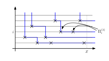
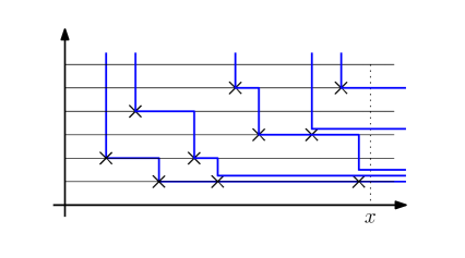
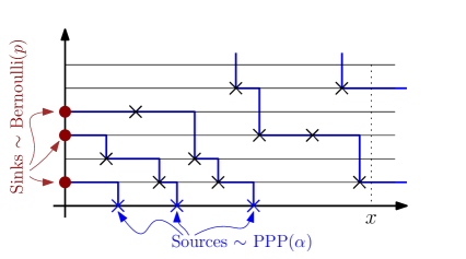
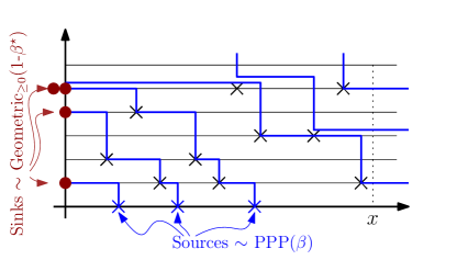
Figure 2: Our four variants of the Hammersley process (time goes from bottom to top, trajectories of particules are indicated in blue). Top left: The process $L_{<}(t)$. Top right: The process $L_{\leq}(t)$. Bottom left: The process $L^{(\alpha,p)}_{<}(t)$. Bottom right: The process $L^{(\beta,\beta^{\star})}_{\leq}(t)$.

Exactly the same way as for the classical Hammersley process ([Ham72, Sec.9], [AD95]) the individual dynamic of particles is very easy to describe:

• The process $L_{<}$ . We put $L_{<}(0)=\emptyset$. In order to define $L_{<}(t+1)$ from $L_{<}(t)$ we consider particles from left to right. A particle at $y$ in $L_{<}(t)$ moves at time $t+1$ at the location of the leftmost available point $z$ in $\Pi_{t+1}^{(\lambda)}\cap(0,y)$ (if any, otherwise it stays at $y$). This point $z$ is not available anymore for subsequent particles, as well as every other point of $\Pi_{t}^{(\lambda)}\cap(0,y)$.
  

  

  If there is a point in $\Pi_{t+1}^{(\lambda)}$ which is on the right of $y^{\prime}:=\max\{L_{<}(t)\}$ then a new particle is created in $L_{<}(t+1)$, located at the leftmost point in $\Pi_{t+1}^{(\lambda)}\cap(y^{\prime},x)$. (In pictures this new particle comes from the right.)
  A realization of $L_{<}$ is shown on top-left of Fig.2.

• The process $L_{\leq}$ . We put $L_{\leq}(0)=\emptyset$. In order to define $L_{\leq}(t+1)$ from $L_{\leq}(t)$ we also consider particles from left to right. A particle at $y$ in $L_{\leq}(t)$ moves at time $t+1$ at the location of the leftmost available point $z$ in $\Pi_{t}^{(\lambda)}\cap(0,y)$. This point $z$ is not available anymore for subsequent particles, other points in $(z,y)$ remain available.
  

  

  If there is a point in $\Pi_{t+1}^{(\lambda)}$ which is on the right of $y^{\prime}:=\max\{L_{<}(t)\}$ then new particles are created in $L_{<}(t+1)$, one for each point in $\Pi_{t+1}^{(\lambda)}\cap(y^{\prime},x)$.
  A realization of $L_{\leq}$ is shown on top-right of Fig.2.

Processes $L_{<}(t)$ and $L_{\leq}(t)$ are designed in such a way that they record the length of longest increasing/non-decreasing paths in $\Pi$. In fact particles trajectories correspond to the level sets of the functions $(x,t)\mapsto\mathcal{L}_{<}\left(\Pi^{(\lambda)}_{x,t}\right)$, $(x,t)\mapsto\mathcal{L}_{\leq}\left(\Pi^{(\lambda)}_{x,t}\right)$.

Proposition 4.

For every $x$,

$$\mathcal{L}_{<}\left(\Pi^{(\lambda)}_{x,t}\right)=\mathrm{card}(L_{<}(t)),\qquad\mathcal{L}_{\leq}\left(\Pi^{(\lambda)}_{x,t}\right)=\mathrm{card}(L_{\leq}(t)),$$

where on each right-hand side we consider the particle system on $[0,x]$.

Proof.

We are merely restating the original construction from Hammersley ([Ham72], Sec.9). We only do the case of $L_{<}(t)$.

Let us call each particle trajectory a Hammersley line. By construction each Hammersley line is a broken line starting from the right of the box $[0,x]\times[0,t]$ and is formed by a succession of north/west line segments. Because of this, two distinct points in a given longest increasing subsequence of $\Pi^{(\lambda)}_{x,t}$ cannot belong to the same Hammersley line. Since there are $L_{<}(t)$ Hammersley’s lines this gives $\mathcal{L}_{<}\left(\Pi^{(\lambda)}_{x,t}\right)\leq\mathrm{card}(L_{<}(t))$.

In order to prove the converse inequality we build from this graphical construction a longest increcreasing subsequence of $\Pi^{(\lambda)}_{x,t}$ with exactly one point on each Hammersley line. To do so, we order Hammersley’s lines from bottom-left to top-right, and we build our path starting from the top-right corner. We first choose any point of $\Pi^{(\lambda)}_{x,t}$ belonging to the last Hammersley line. We then proceed by induction: we choose the next point among the points of of $\Pi^{(\lambda)}_{x,t}$ lying on the previous Hammersley line such that the subsequence remains increasing. (This is possible since Hammersley’s lines only have North/West line segments.) This proves $\mathcal{L}_{<}\left(\Pi^{(\lambda)}_{x,t}\right)\geq\mathrm{card}(L_{<}(t))$. ∎

3.2 Sources and sinks: stationarity

Proposition 4 tells us that in on our way to prove Theorem 1 and Theorem 2 we need to understand the asymptotic behaviour of processes $L_{<},L_{\leq}$. It is proved in [FM06] that the homogeneous PPP with intensity $\alpha$ on $\mathbb{R}$ is stationary for $(L_{<}(t))_{t}$.

However we need non-asymptotic estimates for $(L_{<}(t))_{t}$ (and $(L_{\leq}(t))_{t}$) on a given interval $(0,x)$. To solve this issue we use the trick of sources/sinks introduced formally and exploited by Cator and Groeneboom [CG05] for the continuous HAD process:

• Sources form a finite subset of $[0,x]\times\{0\}$ which plays the role of the initial configuration $L_{<}(0),L_{\leq}(0)$.

• Sinks are points of $\{0\}\times[1,t]$ which add up to $\Pi^{(\lambda)}$ when one defines the dynamics of $L_{<}(t),L_{\leq}(t)$. For $L_{\leq}(t)$ it makes sense to add several sinks at the same location $(0,i)$ so sinks may have a multiplicity.

Examples of dynamics of $L_{<},L_{\leq}$ under the influence of sources/sinks is illustrated at the bottom of Fig.2.

Here is the discrete-time analogous of [CG05, Th.3.1.]:

Lemma 5.

For every $\lambda,\alpha>0$ let $L^{(\alpha,p)}_{<}(t)$ be the Hammersley process defined as $L_{<}(t)$ with:

• sources distributed according to a homogeneous PPP with intensity $\alpha$ on $[0,x]\times\{0\}$ ;

• sinks distributed according to i.i.d. $\mathrm{Bernoulli}(p)$ with

  $$\frac{\lambda}{\lambda+\alpha}=p.$$ (8)

If sources, sinks, and $\Pi^{(\lambda)}$ are independent then the process $\left(L^{(\alpha,p)}_{<}(t)\right)_{t\geq 0}$ is stationary.

Lemma 6.

For every $\beta>\lambda>0$ let $L^{(\beta,\beta^{\star})}_{\leq}(t)$ be the Hammersley process defined as $L_{\leq}(t)$ with:

• sources distributed according to a homogeneous PPP with intensity $\beta$ on $[0,x]\times\{0\}$ ;

• sinks distributed according to i.i.d. $\mathrm{Geometric}_{\geq 0}(1-\beta^{\star})$ with

  $$\beta^{\star}\beta=\lambda.$$ (9)

If sources, sinks, and $\Pi^{(\lambda)}$ are independent then the process $\left(L^{(\beta,\beta^{\star})}_{\leq}(t)\right)_{t\geq 0}$ is stationary.

Proof of Lemmas 5 and 6.

Lemma 6 could be obtain from minor adjustments of [Boy22, Chap.3, Lemma 3.2]. (Be aware that we have to switch $x\leftrightarrow t$ and sources $\leftrightarrow$ sinks in [Boy22] in order to fit our setup.) For the sake of the reader we however propose the following alternative proof which explains where (9) come from.

Consider for some fixed $t\geq 1$ the process $(H_{y})_{0\leq y\leq x}$ given by the number of Hammersley lines passing through the point $(y,t)$.

The initial value $H_{0}$ is the number of sinks at $(0,t)$, which is distributed as a $\mathrm{Geometric}_{\geq 0}(1-\beta^{\star})$. The process $(H_{y})$ is a random walk (reflected at zero) with ’$+1$ rate’ equal to $\lambda$ and ’$-1$ rate’ equal to $\beta$. (Jumps of $(H_{y})$ are independent from sinks as sinks are independent from $\Pi^{(\lambda)}$.) The $\mathrm{Geometric}_{\geq 0}(1-\beta^{\star})$ distribution is stationary for this random walk exactly when (9) holds. The set of points of $L^{(\beta,\beta^{\star})}_{\leq}(t)$ is given by the union of $\Pi_{t}^{(\lambda)}$ and the points of $L^{(\beta,\beta^{\star})}_{\leq}(t)$ that do not correspond to a ’$-1$’ jump. Computations given in Appendix B show that this is distributed as a homogeneous PPP with intensity $\beta$.

Lemma 5 is proved exactly in the same way, calculations are even easier. In this case the corresponding process $(H_{y})_{0\leq y\leq x}$ takes its values in $\{0,1\}$ and its stationary distribution is the Bernoulli distribution with mean $\lambda/(\alpha+\lambda)$, hence (8). ∎

3.3 Processes $L_{<}(t)$ and $L_{\leq}(t)$: non-asymptotic bounds

From Lemmas 5 and 6 it is straightforward to derive non-asymptotic upper bounds for $L_{<}(t),L_{\leq}(t)$.

For $y\leq x$ let ${\sf So}^{(\alpha)}_{x}$ be the random set of sources with intensity $\alpha$ and for $s\leq t$ let ${\sf Si}^{(p)}_{t}$ the random set of sinks with intensity $p$. It is convenient to use the notation $\mathcal{L}_{=<}(\mathcal{P})$ which is, as before, the length of the longest increasing path taking points in $\mathcal{P}$ but when the path is also allowed to go through several sources (which have however the same $y$-coordinate) or several sinks (which have the same $x$-coordinate). Formally,

$$\mathcal{L}_{=<}(\mathcal{P})=\max\left\{L;\hbox{ there exists }P_{1}=\prec P_{2}=\prec\dots=\prec P_{L},\text{ where each }P_{i}\in\mathcal{P}\right\},\\$$

where

$$(x,y)=\prec(x^{\prime},y^{\prime})\text{ if }\begin{cases}&x<x^{\prime}\text{ and }y<y^{\prime},\\ \text{ or }&x=x^{\prime}=0\text{ and }y<y^{\prime},\\ \text{ or }&x<x^{\prime}\text{ and }y=y^{\prime}=0.\end{cases}$$

Proposition 4 can be generalized in

$$\mathcal{L}_{=<}\left(\Pi^{(\lambda)}_{x,t}\cup{\sf So}^{(\alpha)}_{x}\cup{\sf Si}^{(p)}_{t}\right)=L^{(\alpha,p)}_{<}(t)+\mathrm{card}({\sf Si}^{(p)}_{t}).$$ (10)

Lemma 7 (Domination for $\mathcal{L}_{<}$).

For every $\alpha,p\in(0,1)$ such that (8) holds, there is a stochastic domination of the form:

$$\mathcal{L}_{<}\left(\Pi^{(\lambda)}_{x,t}\right)\preccurlyeq\mathrm{Poisson}(x\alpha)+\mathrm{Binomial}(t,p).$$ (11)

(The $\mathrm{Poisson}$ and $\mathrm{Binomial}$ random variables involved in (11) are not independent.)

Proof.

Adding sources and sinks may not decrease longest increasing paths. Thus,

$$\mathcal{L}_{<}\left(\Pi^{(\lambda)}_{x,t}\right) \preccurlyeq\mathcal{L}_{=<}\left(\Pi^{(\lambda)}_{x,t}\cup{\sf So}^{(\alpha)}_{x}\cup{\sf Si}^{(p)}_{t}\right)$$

$$=L^{(\alpha,p)}_{<}(t)+\mathrm{card}({\sf Si}^{(p)})\text{ (using \eqref{prop:NombreLignes_bis})}$$

$$\stackrel{{\scriptstyle\text{(d)}}}{{=}}L^{(\alpha,p)}_{<}(0)+\mathrm{card}({\sf Si}^{(p)})\text{ (using stationarity: Lemma \ref{lem:Stationnaire<})}$$

$$\stackrel{{\scriptstyle\text{(d)}}}{{=}}\mathrm{Poisson}(x\alpha)+\mathrm{Binomial}(t,p).\qed$$

Taking expectations in (11) we obtain

$$\mathbb{E}\left[\mathcal{L}_{<}\left(\Pi^{(\lambda)}_{x,t}\right)\right]\leq x\alpha+tp.$$

As the LHS in the above equation does not depend on $\alpha,p$ (provided that $\alpha,p$ satisfies (8)) we will apply (11) with the minimizing choice

$$\bar{\alpha},\bar{p}:=\mathrm{argmin}_{\alpha,p\text{ satisfying \eqref{eq:alpha_p}}}\left\{x\alpha+tp\right\},$$

i.e.

$$\bar{\alpha}=\sqrt{\frac{t\lambda}{x}}-\lambda,\qquad\bar{p}=\sqrt{\frac{x\lambda}{t}},\qquad x\bar{\alpha}+t\bar{p}=2\sqrt{xt\lambda}-x\lambda.$$ (12)

We have proved

$$\mathbb{E}\left[\mathcal{L}_{<}\left(\Pi^{(\lambda)}_{x,t}\right)\right]\leq 2\sqrt{xt\lambda}-x\lambda.$$

(Compare with (1).) We have a similar statement for non-decreasing subsequences:

Lemma 8 (Domination for $\mathcal{L}_{\leq}$).

For every $\beta,\beta^{\star}\in(0,1)$ such that (9) holds, there is a stochastic domination of the form:

$$\mathcal{L}_{\leq}\left(\Pi^{(\lambda)}_{x,t}\right)\preccurlyeq\mathrm{Poisson}(x\beta)+\mathcal{G}_{1}^{(\beta^{\star})}+\dots+\mathcal{G}_{t}^{(\beta^{\star})},$$ (13)

where $\mathcal{G}_{i}^{(\beta^{\star})}$’s are i.i.d. $\mathrm{Geometric}_{\geq 0}(1-\beta^{\star})$.

We put

$$\bar{\beta},\bar{\beta}^{\star}:=\mathrm{argmin}_{\beta,\beta^{\star}\text{ satisfying \eqref{eq:alpha}}}\left\{x\beta+t\left(\frac{\beta^{\star}}{1-\beta^{\star}}\right)\right\},$$ (14)

i.e.

$$\bar{\beta}=\sqrt{\frac{t\lambda}{x}}+\lambda,\qquad\bar{\beta}^{\star}=\frac{1}{1+\sqrt{t/x\lambda}},\qquad x\bar{\beta}+t\left(\frac{\bar{\beta}}{1-\bar{\beta}}\right)=2\sqrt{xt\lambda}+x\lambda.$$ (15)

(In particular $\bar{\beta}>\lambda$, as required in Lemma 6.) Eq.(13) yields

$$\mathbb{E}\left[\mathcal{L}_{\leq}\left(\Pi^{(\lambda)}_{x,t}\right)\right]\leq 2\sqrt{xt\lambda}+x\lambda.$$ (16)

(Compare with (2).)

Theorem 9 (Concentration for $\mathcal{L}_{<}$, $\mathcal{L}_{\leq}$).

There exist strictly positive functions $g,h$ such that for all $\varepsilon>0$ and for every $x,t,\lambda$ such that $t\geq x\lambda$

$$\mathbb{P}(\mathcal{L}_{<}(\Pi^{(\lambda)}_{x,t}) >(1+\varepsilon)(2\sqrt{xt\lambda}-x\lambda))\leq\exp(-g(\varepsilon)(\sqrt{xt\lambda}-x\lambda)),$$ (17)

$$\mathbb{P}(\mathcal{L}_{<}(\Pi^{(\lambda)}_{x,t}) <(1-\varepsilon)(2\sqrt{xt\lambda}-x\lambda))\leq\exp(-h(\varepsilon)(\sqrt{xt\lambda}-x\lambda)).$$ (18)

Similarly:

$$\mathbb{P}(\mathcal{L}_{\leq}(\Pi^{(\lambda)}_{x,t}) >(1+\varepsilon)(2\sqrt{xt\lambda}+x\lambda))\leq\exp(-g(\varepsilon)\sqrt{xt\lambda}),$$ (19)

$$\mathbb{P}(\mathcal{L}_{\leq}(\Pi^{(\lambda)}_{x,t}) <(1-\varepsilon)(2\sqrt{xt\lambda}+x\lambda))\leq\exp(-h(\varepsilon)\sqrt{xt\lambda}).$$ (20)

For the proof of Theorem 9 we will focus on the case of $\mathcal{L}_{<}$, i.e. eq.(17), (18). When necessary we will give the slight modification needed to prove eq.(19) and (20). The beginning of the proof mimics Lemmas 4.1 and 4.2 in [BEGG16].

We first prove similar bounds for the stationary processes with minimizing sources and sinks.

Lemma 10 (Concentration for $\mathcal{L}_{<}$ with sources and sinks).

Let $\bar{\alpha},\bar{p}$ be defined by (12). There exists a strictly positive function $g_{1}$ such that for all $\varepsilon>0$ and for every $x,t,\lambda$ such that $t\geq x\lambda$

$$\mathbb{P}(\mathcal{L}_{=<}(\Pi^{(\lambda)}_{x,t}\cup{\sf So}^{(\bar{\alpha})}_{x}\cup{\sf Si}^{(\bar{p})}_{t}) >(1+\varepsilon)(2\sqrt{xt\lambda}-x\lambda))\leq 2\exp(-g_{1}(\varepsilon)(\sqrt{xt\lambda}-x\lambda))$$ (21)

$$\mathbb{P}(\mathcal{L}_{=<}(\Pi^{(\lambda)}_{x,t}\cup{\sf So}^{(\bar{\alpha})}_{x}\cup{\sf Si}^{(\bar{p})}_{t}) <(1-\varepsilon)(2\sqrt{xt\lambda}-x\lambda))\leq 2\exp(-g_{1}(\varepsilon)(\sqrt{xt\lambda}-x\lambda)).$$ (22)

Proof of Lemma 10.

By stationarity (Lemma 5) we have

$$\mathcal{L}_{=<}(\Pi^{(\lambda)}_{x,t}\cup{\sf So}^{(\bar{\alpha})}_{x}\cup{\sf Si}^{(\bar{p})}_{t})\overset{(d)}{=}\mathrm{Poisson}(x\bar{\alpha})+\mathrm{Binomial}(t,\bar{p}).$$

Then

$$\mathbb{P}(\mathcal{L}_{=<}(\Pi^{(\lambda)}_{x,t}\cup{\sf So}^{(\bar{\alpha})}_{x}\cup{\sf Si}^{(\bar{p})}_{t}>(1+\varepsilon)(2\sqrt{xt\lambda}-x\lambda))\leq \ \mathbb{P}\left(\mathrm{Poisson}(x\bar{\alpha})>(1+\frac{\varepsilon}{2})(\sqrt{xt\lambda}-x\lambda)\right)$$

$$+ \ \mathbb{P}\left(\mathrm{Binomial}(t,\bar{p})>(1+\frac{\varepsilon}{2})\sqrt{xt\lambda}\right).$$

Recall that $x\bar{\alpha}=\sqrt{xt\lambda}-x\lambda$, $t\bar{p}=\sqrt{xt\lambda}$. Using the tail inequality for the Poisson distribution (Lemma 15):

$$\mathbb{P}\left(\mathrm{Poisson}(x\bar{\alpha})>(1+\frac{\varepsilon}{2})(\sqrt{xt\lambda}-x\lambda)\right) \leq\exp\left(-(\sqrt{xt\lambda}-x\lambda)\varepsilon^{2}/4\right)$$

Using the tail inequality for the binomial (Lemma 16) we get

$$\mathbb{P}\left(\mathrm{Binomial}(t,\bar{p})>(1+\frac{\varepsilon}{2})\sqrt{xt\lambda}\right)\leq\exp(-\tfrac{1}{12}\varepsilon^{2}\sqrt{xt\lambda})\leq\exp(-\tfrac{1}{12}\varepsilon^{2}(\sqrt{xt\lambda}-x\lambda))$$

The proof of (22) is identical. This shows Lemma 10 with $g_{1}(\varepsilon)=\varepsilon^{2}/12$. ∎

For longest non-decreasing subsequences we have a statement similar to Lemma 10. The only modification in the proof is that in order to estimate the number of sinks one has to replace Lemma 16 (tail inequality for the Binomial) by Lemma 17 (tail inequality for a sum of geometric random variables). During the proof we need to bound $\sqrt{xt\lambda}+x\lambda$ by $\sqrt{xt\lambda}$, this explains the form of the right-hand side in eq.(19) and (20).

Proof of Theorem 9.

Adding sources/sinks may not decrease $\mathcal{L}_{<}$ so

$$\mathcal{L}_{=<}(\Pi^{(\lambda)}_{x,t}\cup{\sf So}^{(\bar{\alpha})}_{x}\cup{\sf Si}^{(\bar{p})}_{t})\succcurlyeq\mathcal{L}_{<}(\Pi^{(\lambda)}_{x,t}),$$

thus the upper bound (17) is a direct consequence of Lemma 10.

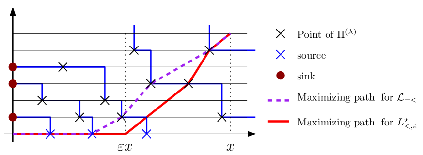
Figure 3: A sample of $\Pi^{(\lambda)}_{x,t}$, sources, sinks, and the corresponding trajectories of particles (in blue). Here $\mathcal{L}_{=<}(\Pi^{(\lambda)}_{x,t}\cup{\sf So}^{(\alpha)}_{x}\cup{\sf Si}^{(p)}_{t})=5$ (pink path) and $L^{(\alpha,p)}_{<}(t)=2$ (two remaining particles at the top of the box).

Let us now prove the lower bound. We consider the length of a maximizing path among those using sources from $0$ to $\varepsilon x$ and then only increasing points of $\Pi^{(\lambda)}_{x,t}\cap\left([\varepsilon x,x]\times[0,t]\right)$ (see Fig.3). Formally we set

$$L_{=<,\varepsilon}^{\star}:=\mathrm{card}\left({\sf So}^{(\bar{\alpha})}_{\varepsilon x}\right)+\mathcal{L}_{<}\left((\Pi^{(\lambda)}_{x,t}\cap\left([\varepsilon x,x]\times[0,t]\right)\right)\stackrel{{\scriptstyle\text{(d)}}}{{=}}\mathrm{Poisson}(\varepsilon x\bar{\alpha})+\mathcal{L}_{<}\left((\Pi^{(\lambda)}_{x,t}\cap\left([\varepsilon x,x]\times[0,t]\right)\right)$$ (23)

The idea is that for any fixed $\varepsilon$ the paths contributing to $L_{=<,\varepsilon}^{\star}$ will typically not contribute to $\mathcal{L}_{=<}\left(\Pi^{(\lambda)}_{x,t}\cup{\sf So}^{(\bar{\alpha})}_{x}\cup{\sf Si}^{(\bar{p})}_{t}\right)=L^{(\bar{\alpha},p)}_{<}(t)+\mathrm{card}({\sf Si}^{(\bar{p})}_{t})$. Indeed eq.(23) suggests that for large $x,t$

$$L_{=<,\varepsilon}^{\star} \approx\mathbb{E}[\mathrm{Poisson}(\varepsilon x\bar{\alpha})]+\mathbb{E}\left[\mathcal{L}_{<}\left(\Pi^{(\lambda)}_{x,t}\cap\left([\varepsilon x,x]\times[0,t]\right)\right)\right]$$

$$\approx x\varepsilon\bar{\alpha}+2\sqrt{x(1-\varepsilon)\lambda t}-x(1-\varepsilon)\lambda$$

$$=2\sqrt{x\lambda t}-x\lambda-\sqrt{xt\lambda}\delta(\varepsilon),$$

where $\delta(\varepsilon)=2-\varepsilon-2\sqrt{1-\varepsilon}$ is positive and increasing. In order to make the above approximation rigorous we first write

$$2\sqrt{x\lambda t}-x\lambda-\tfrac{1}{2}\sqrt{xt\lambda}\delta(\varepsilon)=x\varepsilon\bar{\alpha}+\tfrac{1}{4}\sqrt{xt\lambda}\delta(\varepsilon)+2\sqrt{x(1-\varepsilon)\lambda t}-x(1-\varepsilon)\lambda+\tfrac{1}{4}\sqrt{xt\lambda}\delta(\varepsilon).$$ (24)

Combining (23) and (24) gives

$$\mathbb{P}\left(L_{<,\varepsilon}^{\star}\geq 2\sqrt{x\lambda t}-x\lambda-\tfrac{1}{2}\sqrt{xt\lambda}\delta(\varepsilon)\right)$$

$$\leq \ \mathbb{P}\left(\mathrm{Poisson}(x\varepsilon\bar{\alpha})\geq x\varepsilon\bar{\alpha}+\tfrac{1}{4}\sqrt{xt\lambda}\delta(\varepsilon)\right)$$

$$+ \ \mathbb{P}\left(\mathcal{L}_{<}(\Pi^{(\lambda)}_{x,t}\cap\left([\varepsilon x,x]\times[0,t]\right)\geq 2\sqrt{x(1-\varepsilon)\lambda t}-x(1-\varepsilon)\lambda+\tfrac{1}{4}\sqrt{xt\lambda}\delta(\varepsilon)\right)$$

$$\leq \ \exp\left(-\frac{xt\lambda\delta(\varepsilon)^{2}}{16\times 4\varepsilon^{2}(\sqrt{xt\lambda}-x\lambda)}\right)\qquad\text{(using Lemma \ref{lem:Chernov})}$$

$$+ \ \mathbb{P}\left(\mathcal{L}_{<}(\Pi^{(\lambda)}_{x,t}\cap\left([\varepsilon x,x]\times[0,t]\right)\geq 2\sqrt{x(1-\varepsilon)\lambda t}-x(1-\varepsilon)\lambda+\tfrac{1}{8}(2\sqrt{x(1-\varepsilon)\lambda t}-x(1-\varepsilon)\lambda)\delta(\varepsilon)\right)$$

$$\leq \ \exp\left(-\sqrt{xt\lambda}\delta(\varepsilon)^{2}/(64\varepsilon^{2})\right)$$

$$+ \ \mathbb{P}\left(\mathcal{L}_{<}(\Pi^{(\lambda)}_{x,t}\cap\left([\varepsilon x,x]\times[0,t]\right)\geq\left(2\sqrt{x(1-\varepsilon)\lambda t}-x(1-\varepsilon)\lambda\right)\times(1+\tfrac{1}{8}\delta(\varepsilon))\right)$$

$$\leq \ \exp\left(-\sqrt{xt\lambda}\delta(\varepsilon)^{2}/(64\varepsilon^{2})\right)$$

$$\ +\exp\left(-g(\delta(\varepsilon)/8)(\sqrt{x(1-\varepsilon)t\lambda}-x(1-\varepsilon)\lambda)\right)\text{(using the upper bound \eqref{eq:upper})}$$

and thus we can find some positive $h$ such that

$$\mathbb{P}\left(L_{<,\varepsilon}^{\star}\geq 2\sqrt{x\lambda t}-x\lambda-\tfrac{1}{2}\sqrt{xt\lambda}\delta(\varepsilon)\right)\leq\exp\left(-h(\varepsilon)(\sqrt{xt\lambda}-x\lambda)\right).$$ (25)

One proves exactly in the same way a similar bound for the length of a maximizing path among those using sinks in $\{0\}\times[0,\varepsilon t]$ and then only increasing points of $\Pi^{(\lambda)}_{x,t}\cap\left([0,x]\times[\varepsilon t,t]\right)$.

Choose now one of the maximizing paths $\mathcal{P}$ for $\mathcal{L}_{=<}\left(\Pi^{(\lambda)}_{x,t}\cup{\sf So}^{(\bar{\alpha})}_{x}\cup{\sf Si}^{(\bar{p})}_{t}\right)$ (if there are many of them, choose one arbitrarily in a deterministic way: the lowest, say). Denote by ${\sf sources}(\mathcal{P})$ and ${\sf sinks}(\mathcal{P})$ the number of sources and sinks in the path $\mathcal{P}$:

$${\sf sources}(\mathcal{P})=\mathrm{card}\left\{0\leq y\leq x\text{ such that }(y,0)\in\mathcal{P}\right\}.$$

In Fig.3 the path $\mathcal{P}$ is sketched in pink and ${\sf sources}(\mathcal{P})=2$, ${\sf sinks}(\mathcal{P})=0$.

Lemma 11.

There exists a positive function $\psi$ such that for all real $\eta>0$

$$\mathbb{P}\left({\sf sources}(\mathcal{P})+{\sf sinks}(\mathcal{P})\geq\eta\sqrt{x\lambda t}\right)\leq 2\exp(-\psi(\eta)(\sqrt{x\lambda t}-x\lambda)).$$

Proof of Lemma 11.

If the event $\left\{{\sf sources}(\mathcal{P})\geq\eta\sqrt{x\lambda t}\right\}$ holds then there exists a (random) $\varepsilon$ such that the two following events hold:

• ${\sf So}_{\varepsilon x}\geq\eta\sqrt{x\lambda t}$ ;

• $L_{=<,\varepsilon}^{\star}=\mathcal{L}_{=<}\left(\Pi^{(\lambda)}_{x,t}\cup{\sf So}^{(\bar{\alpha})}_{x}\cup{\sf Si}^{(\bar{p})}_{t}\right)=L^{(\bar{\alpha},\bar{p})}_{<}(t)+\mathrm{card}({\sf Si}^{(\bar{p})}_{t})$.

This implies that this random $\varepsilon$ is larger than $\eta/2>0$ unless the number of sources in $[0,x\eta/2]$ is improbably high:

$$\mathbb{P}({\sf sources}(\mathcal{P})\geq\eta\sqrt{x\lambda t})\leq \ \mathbb{P}({\sf So}_{\eta x/2}\geq\eta\sqrt{x\lambda t})+\mathbb{P}({\sf sources}(\mathcal{P})\geq\eta\sqrt{x\lambda t};\ {\sf So}_{\eta x/2}<\eta\sqrt{x\lambda t})$$

$$\leq \ \mathbb{P}({\sf So}_{\eta x/2}\geq\eta\sqrt{x\lambda t})$$

$$+ \ \mathbb{P}(L^{(\bar{\alpha},\bar{p})}_{<}(t)\leq\sqrt{x\lambda t}-x\lambda-\tfrac{1}{4}\delta(\eta/3)\sqrt{x\lambda t})$$

$$+ \ \mathbb{P}(\mathrm{card}({\sf Si}^{(\bar{p})}_{t})\leq\sqrt{x\lambda t}-\tfrac{1}{4}\delta(\eta/3)\sqrt{x\lambda t})$$

$$+ \ \mathbb{P}(L_{=<,\varepsilon}^{\star}\geq 2\sqrt{x\lambda t}-x\lambda-\tfrac{1}{2}\delta(\eta/3)\sqrt{x\lambda t}\text{ for some }\eta/2\leq\varepsilon\leq 1).$$

From previous calculations, the three first terms in the above display are less than $\exp(-\phi(\eta)(\sqrt{x\lambda t}-x\lambda))$ for some positive function $\phi$. To conclude the proof it remains to bound the fourth term. Let $K$ be an integer larger than $6/\eta^{3}$, by definition of $L_{=<,\varepsilon}^{\star}$ we have for every $\varepsilon\in[\tfrac{k}{K},\tfrac{k+1}{K})$

$$L_{=<,\varepsilon}^{\star}\leq L_{=<,k/K}^{\star}+\mathrm{card}({\sf So}^{(\bar{\alpha})}_{x}\cap[\tfrac{k}{K},\tfrac{k+1}{K}]).$$

Thus

$$\mathbb{P}(\bigcup_{\eta/2\leq\varepsilon\leq 1} L_{=<,\varepsilon}^{\star}>2\sqrt{x\lambda t}-x\lambda-\tfrac{1}{2}\delta(\eta/3)\sqrt{x\lambda t})$$

$$\leq \sum_{k\geq\lfloor\eta K/2\rfloor}\mathbb{P}\left(L_{=<,k/K}^{\star}>2\sqrt{x\lambda t}-x\lambda-\delta(\eta/3)\sqrt{x\lambda t}\right)$$

$$+ \sum_{k\geq\lfloor\eta K/2\rfloor}\mathbb{P}\left(\mathrm{card}({\sf So}^{(\bar{\alpha})}_{x}\cap[\tfrac{k}{K},\tfrac{k+1}{K}])>\tfrac{1}{2}\delta(\eta/3)\sqrt{x\lambda t}\right)$$

$$\leq \sum_{k\geq\lfloor\eta K/2\rfloor}\mathbb{P}\left(L_{=<,k/K}^{\star}>2\sqrt{x\lambda t}-x\lambda-\delta(k/K)\sqrt{x\lambda t}\right)\quad\text{ (since $K>6/\eta^{3}>6/\eta$ and $\delta$ is increasing)}$$

$$+ \sum_{k\geq\lfloor\eta K/2\rfloor}\mathbb{P}\left(\mathrm{card}({\sf So}^{(\bar{\alpha})}_{x}\cap[\tfrac{k}{K},\tfrac{k+1}{K}])>\tfrac{1}{2}\delta(\eta/3)\sqrt{x\lambda t}\right)$$

$$\leq \sum_{k\geq\lfloor\eta K/2\rfloor}\exp(-h(k/K)(\sqrt{xt\lambda}-x\lambda))\qquad\text{ (using \eqref{eq:Majo_Leps})}$$

$$+ K\times\mathbb{P}\left(\mathrm{Poisson}(\bar{\alpha}/K)>\tfrac{1}{2}\delta(\eta/3)\sqrt{x\lambda t}\right)$$

$$\leq \ K\exp(-h(\eta/3)(\sqrt{xt\lambda}-x\lambda))+K\times\mathbb{P}\left(\mathrm{Poisson}(\bar{\alpha}/K)>\tfrac{1}{2}\delta(\eta/3)\sqrt{x\lambda t}\right),$$

$$\leq \ K\exp(-h(\eta/3)(\sqrt{xt\lambda}-x\lambda))+K\times\mathbb{P}\left(\mathrm{Poisson}(\bar{\alpha}/K)>\bar{\alpha}/K+\frac{\eta^{2}}{32}\sqrt{x\lambda t}\right),\quad\text{ (using $K>6/\eta^{3}$)}$$

$$\leq \frac{12}{\eta}\exp(-\varphi(\eta)(\sqrt{xt\lambda}-x\lambda)),$$

for some positive function $\varphi(\eta)$. We can find $\psi$ such that

$$\min\left\{1,\frac{12}{\eta}e^{-\varphi(\eta)(\sqrt{xt\lambda}-x\lambda)}+3\exp(-\phi(\eta))\right\}\leq e^{-\psi(\eta)(\sqrt{xt\lambda}-x\lambda)}$$

and thus $\mathbb{P}({\sf sources}(\mathcal{P})\geq\eta\sqrt{x\lambda t})\leq\exp(-\psi(\eta)(\sqrt{xt\lambda}-x\lambda))$. With minor modifications one proves the same bound for sinks (possibly by changing $\psi$): $\mathbb{P}({\sf sinks}(\mathcal{P})\geq\eta\sqrt{x\lambda t})\leq\exp(-\psi(\eta)(\sqrt{xt\lambda}-x\lambda))$ and Lemma 11 is proved. ∎

We can conclude the proof of the lower bound in Theorem 9. Let us write

$$L_{<}(t)\geq\mathcal{L}_{=<}(\Pi^{(\lambda)}_{x,t}\cup{\sf So}^{(\bar{\alpha})}_{x}\cup{\sf Si}^{(\bar{p})}_{t})-{\sf sources}(\mathcal{P})-{\sf sinks}(\mathcal{P}),$$

we bound the right-hand side using Lemmas 10 and 11. ∎

4 Proof of Theorem 1 when $k_{n}\to+\infty$: de-Poissonization

In order to conclude the proof of Theorem 1 it remains to de-Poissonize Theorem 9. We need a few notation. For any integers $i_{1},\dots,i_{n}$ let $\mathcal{S}_{i_{1},\dots,i_{n}}$ be the random set of points given by $i_{\ell}$ uniform points on each horizontal line:

$$\mathcal{S}_{i_{1},\dots,i_{n}}=\cup_{\ell=1}^{n}\cup_{r=1}^{i_{\ell}}\left\{U_{\ell,r}\right\}\times\left\{\ell\right\},$$

where $(U_{\ell,r})_{\ell,r}$ is an array of i.i.d. uniform random variables in $[0,1]$. Set also $e_{i_{1},\dots,i_{n}}=\mathbb{E}[\mathcal{L}_{<}(\mathcal{S}_{i_{1},\dots,i_{n}})].$ By uniformity of $U$’s we have the identity $\mathbb{E}[\mathcal{L}_{<}(S_{k;n})]=e_{k,\dots,k}$ and therefore our problem reduces to estimating $e_{k,\dots,k}$. On the other hand if $X_{1},\dots,X_{n}$ are i.i.d. Poisson random variables with mean $k$ then

$$\mathbb{E}[e_{X_{1},\dots,X_{n}}]=\mathbb{E}\left[\mathcal{L}_{<}(\mathcal{P}_{nk_{n},n}^{(1/n)})\right]=2\sqrt{nk_{n}}-k_{n}+o(\sqrt{nk_{n}}).$$ (26)

The last equality is obtained by combining Theorem 9 for

$$x=nk_{n},\qquad t=n,\qquad\lambda_{n}=\frac{1}{n}$$

with the trivial bound $\mathcal{L}_{<}(\mathcal{P}_{nk_{n},n}^{(1/n)})\leq n$. In order to exploit (26) we need the following smoothness estimate.

Lemma 12.

For every $i_{1},\dots,i_{n}$ and $j_{1},\dots,j_{n}$

$$\left|e_{i_{1},\dots,i_{n}}-e_{j_{1},\dots,j_{n}}\right|\leq 6\sqrt{\sum_{\ell=1}^{n}|i_{\ell}-j_{\ell}|}.$$

Proof.

Let $\mathcal{S}=\mathcal{S}_{i_{1},\dots,i_{n}}$ be as above. If we replace in $\mathcal{S}$ the $y$-coordinate of each point of the form $(x,\ell)$ by a new $y$-coordinate uniform in the interval $(\ell,\ell+1)$ (independent from anything else) then this defines a uniform permutation $\sigma_{i_{1}+\dots+i_{n}}$ of size $i_{1}+\dots+i_{n}$. The longest increasing subsequence in $\mathcal{S}$ is mapped onto an increasing subsequence in $\sigma_{i_{1}+\dots+i_{n}}$ and thus this construction shows the stochastic domination $\mathcal{L}_{<}(\mathcal{S}_{i_{1},\dots,i_{n}})\preccurlyeq\mathcal{L}_{<}(\sigma_{i_{1}+\dots+i_{n}}).$ Thus for every $i_{1},\dots,i_{n}$,

$$e_{i_{1},\dots,i_{n}}\leq\mathbb{E}[\mathcal{L}_{<}(\sigma_{i_{1}+\dots+i_{n}})]\leq 6\sqrt{i_{1}+\dots+i_{n}}.$$ (27)

(The last inequality follows from [Ste97, Lemma 1.4.1].) Besides, consider for two $n$-tuples $i_{1},\dots,i_{n}$ and $j_{1},\dots,j_{n}$ two independent set of points $\mathcal{S}_{i_{1},\dots,i_{n}}$, $\widetilde{\mathcal{S}}_{j_{1},\dots,j_{n}}$ then

$$\mathcal{L}_{<}(\mathcal{S}_{i_{1},\dots,i_{n}})\leq\mathcal{L}_{<}(\mathcal{S}_{i_{1},\dots,i_{n}}\cup\widetilde{\mathcal{S}}_{j_{1},\dots,j_{n}})\leq\mathcal{L}_{<}(\mathcal{S}_{i_{1},\dots,i_{n}})+\mathcal{L}_{<}(\widetilde{\mathcal{S}}_{j_{1},\dots,j_{n}}).$$

This proves that

$$e_{i_{1},\dots,i_{n}}\leq e_{i_{1}+j_{1},\dots,i_{n}+j_{n}}\leq e_{i_{1},\dots,i_{n}}+e_{j_{1},\dots,j_{n}}.$$

(In particular $(i_{1},\dots,i_{n})\mapsto e_{i_{1},\dots,i_{n}}$ is non-decreasing with respect to any of its coordinate.) Therefore

$$e_{i_{1},\dots,i_{n}} \leq e_{(i_{1}-j_{1})^{+},\dots,(i_{n}-j_{n})^{+}}+e_{j_{1}-(i_{1}-j_{1})^{-},\dots,j_{n}-(i_{n}-j_{n})^{-}}$$

$$\leq e_{|i_{1}-j_{1}|,\dots,|i_{n}-j_{n}|}+e_{j_{1},\dots,j_{n}}.$$

By switching the role of $i$’s and $j$’s:

$$|e_{i_{1},\dots,i_{n}}-e_{j_{1},\dots,j_{n}}|\leq e_{|i_{1}-j_{1}|,\dots,|i_{n}-j_{n}|}\leq 6\sqrt{\sum_{\ell=1}^{n}|i_{\ell}-j_{\ell}|},$$

using (27). ∎

Proof of Theorem 1 for any sequence $(k_{n})\to+\infty$.

Using smoothness we write

$$|e_{k,\dots,k}-\mathbb{E}[e_{X_{1},\dots,X_{n}}]|\leq\mathbb{E}\left[|e_{k,\dots,k}-e_{X_{1},\dots,X_{n}}|\right]\leq 6\times\mathbb{E}\left[\left(\sum_{\ell=1}^{n}|X_{\ell}-k|\right)^{1/2}\right].$$ (28)

Using twice the Cauchy-Schwarz inequality:

$$\mathbb{E}\left[\left(\sum_{\ell=1}^{n}|X_{\ell}-k|\right)^{1/2}\right] \leq\sqrt{\mathbb{E}\left[\sum_{\ell=1}^{n}|X_{\ell}-k|\right]}$$

$$\leq\sqrt{n\mathbb{E}\left[|X_{1}-k|\right]}$$

$$\leq\sqrt{n\mathbb{E}\left[|X_{1}-k|^{2}\right]^{1/2}}=\sqrt{n\sqrt{\mathrm{Var}(X_{1})}}=\sqrt{n\sqrt{k}}.$$

If $k=k_{n}\to\infty$ then the last display is a $o(\sqrt{nk_{n}})$ and eq.(28) and (26) show that

$$e_{k,\dots,k}=\mathbb{E}[\mathcal{L}_{<}(S_{k;n})]=2\sqrt{nk_{n}}-k_{n}+o(\sqrt{nk_{n}}).$$

∎

5 Proof of Theorem 2

5.1 Proof for large $(k_{n})$

We now prove Theorem 2 for a large sequence $(k_{n})$. We say that $(k_{n})$ is large if

$$n^{2}k_{n}\exp(-(k_{n})^{\alpha})=\mathrm{o}(\sqrt{nk_{n}})$$ (29)

for some $\alpha\in(0,1)$. Note that $k_{n}=\log n$ is not large while $k_{n}=(\log n)^{1+\varepsilon}$ is large.

We first observe that de-Poissonization cannot be applied as in the previous section. We lack smoothness as, for instance, $\mathbb{E}[\mathcal{L}_{\leq}(\mathcal{S}_{i_{1},0,0,\dots,0})]=i_{1}\neq\mathcal{O}(\sqrt{\sum i_{\ell}})$. The strategy is to apply Theorem 9 with

$$x=nk_{n},\qquad t=n,\qquad\lambda_{n}\approx\frac{1}{n}.$$

(The exact value of $\lambda_{n}$ will be different for the proofs of the lower and upper bounds.)

Proof of the upper bound of (2) for large $(k_{n})$.

Choose $\alpha$ such that $n^{2}k_{n}\exp(-k_{n}^{\alpha})=\mathrm{o}(\sqrt{nk_{n}})$. Put

$$\lambda_{n}=\frac{1}{n}+\frac{\delta_{n}}{n},\qquad\text{ with }\delta_{n}=k_{n}^{-(1-\alpha)/2}.$$

Let $E_{n}^{\lambda_{n}}$ be the event

$$E_{n}^{\lambda_{n}}=\left\{\text{ at least $k_{n}$ points in each row of }\mathcal{P}_{nk_{n},n}^{(\lambda_{n})}\right\}.$$

The event $E_{n}$ occurs with large probability. Indeed,

$$1-\mathbb{P}(E_{n}^{\lambda_{n}}) \leq n\mathbb{P}\left(\mathrm{Poisson}(nk_{n}\lambda_{n})\leq k_{n}\right)$$

$$\leq n\mathbb{P}\left(\mathrm{Poisson}(nk_{n}\lambda_{n})\leq nk_{n}\lambda_{n}+k_{n}-nk_{n}\lambda_{n}\right)$$

$$\leq n\mathbb{P}\left(\mathrm{Poisson}(nk_{n}\lambda_{n})\leq nk_{n}\lambda_{n}-k_{n}\delta_{n}\right)$$

$$\leq n\exp\left(-\frac{k_{n}^{2}\delta_{n}^{2}}{4nk_{n}\lambda_{n}}\right)\leq n\exp\left(-\tfrac{1}{8}k_{n}\delta_{n}^{2}\right)=n\exp\left(-\tfrac{1}{8}k_{n}^{\alpha}\right).$$ (30)

At the last line we used Lemma 15. The latter probability tends to $0$ as $(k_{n})$ is large.

Lemma 13.

Random sets $S_{k_{n};n}$ and $\Pi_{nk_{n},n}^{(\lambda_{n})}$ can be defined on the same probability space in such a way that

$$\mathcal{L}_{\leq}(S_{k_{n};n}) \leq\mathcal{L}_{\leq}(\Pi_{nk_{n},n}^{(\lambda_{n})})+nk_{n}(1-\mathbf{1}_{E_{n}^{\lambda_{n}}}).$$ (31)

Proof of Lemma 13.

Draw a sample of $\Pi_{nk_{n},n}^{(\lambda_{n})}$ and let $\tilde{\Pi}_{nk_{n},n}^{(\lambda_{n})}$ be the subset of $\Pi_{nk_{n},n}^{(\lambda_{n})}$ obtained by keeping only the $k_{n}$ leftmost points in each row. If $E_{n}^{\lambda_{n}}$ occurs then the relative orders of points in $\tilde{\Pi}_{nk_{n},n}^{(\lambda_{n})}$ corresponds to a uniform $k_{n}$-multiset permutation. If $E_{n}^{\lambda_{n}}$ does not hold we bound $\mathcal{L}_{\leq}(S_{k_{n};n})$ by the worst case $nk_{n}$. ∎

Taking expectations in (31) and using the upper bound (16) yields

$$\mathbb{E}[\mathcal{L}_{\leq}(S_{k_{n};n})] \leq 2\sqrt{nk_{n}(1+\delta_{n})}+k_{n}(1+\delta_{n})+n^{2}k_{n}\exp\left(-k_{n}^{\alpha}\right),$$

hence the upper bound in (2).

Proof of the lower bound of (2) for large $(k_{n})$. Choose now $\lambda_{n}=\frac{1}{n}(1-\delta_{n})$ with $\delta_{n}=k_{n}^{-(1-\alpha)/2}$. Let $F_{n}$ be the event

$$F_{n}^{\lambda_{n}}=\left\{\text{ at most $k_{n}$ points in each row of }\mathcal{P}_{nk_{n},n}^{(\lambda_{n})}\right\}.$$

The event $F_{n}^{\lambda_{n}}$ occurs with large probability:

$$1-\mathbb{P}(F_{n}^{\lambda_{n}})\leq n\mathbb{P}\left(\mathrm{Poisson}(nk_{n}\lambda_{n})\geq k_{n}\right)\leq n\exp\left(-\tfrac{1}{8}k_{n}^{\alpha}\right),$$

which tends to zero. Random sets $S_{k_{n};n}$ and $\mathcal{P}_{nk_{n},n}^{(\lambda_{n})}$ can be defined on the same probability space in such a way that

$$\mathcal{L}_{\leq}(S_{k_{n};n}) \geq\mathcal{L}_{\leq}(\mathcal{P}_{nk_{n},n}^{(\lambda_{n})})\mathbf{1}_{F_{n}^{\lambda_{n}}}.$$

Therefore

$$\mathbb{P}\left(\mathcal{L}_{\leq}(S_{k_{n};n})<(2\sqrt{nk_{n}(1-\delta_{n})}+k_{n}(1-\delta_{n}))(1-\varepsilon)\right)\leq\\ \mathbb{P}\left(\mathcal{L}_{\leq}(\mathcal{P}_{nk_{n},n}^{(\lambda_{n})})<(2\sqrt{nk_{n}(1-\delta_{n})}+k_{n}(1-\delta_{n}))(1-\varepsilon)\right)+\mathbb{P}\left(\text{not }F_{n}^{\lambda_{n}}\right).$$ (32)

and we conclude with (20).

5.2 The gap between small and large $(k_{n})$: Conclusion of the proof of Theorem 2

After I circulated a preliminary version of this article, Valentin Féray came up with a simple argument for bridging the gap between small and large $(k_{n})$. This allows to prove Theorem 2 for an arbitrary sequence $(k_{n})$, I reproduce his argument here with his permission.

Lemma 14.

Let $n,k,A$ be positive integers. Two random uniform multiset permutations $\widetilde{S}_{kA;\lfloor n/A\rfloor}$ and $S_{k;n}$ can be built on the same probability space in such a way that

$$\mathcal{L}_{\leq}\left(S_{k;n}\right)\leq\mathcal{L}_{\leq}\left(\widetilde{S}_{kA;\lfloor n/A\rfloor}\right)+kA.$$

Proof of Lemma 14 .

Draw $S_{k;n}$ uniformly at random, the idea is to group all points of $S_{k;n}$ whose height is between $1$ and $A$, to group all points whose height is between $A+1$ and $2A$, and so on.

Formally, denote by $1\leq i_{1}<i_{2}<\dots<i_{kA\lfloor n/A\rfloor}$ the indices such that $1\leq i_{\ell}\leq\lfloor n/A\rfloor$ for every $\ell$ (see Fig.4). For $1\leq\ell\leq kA\lfloor n/A\rfloor$ put

$$\widetilde{S}(\ell)=\lceil S(i_{\ell})/k\rceil.$$

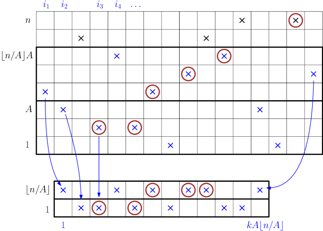
Figure 4: Illustration of the notation of Lemma 14. Top: the multiset permutation $S_{k;n}$. Bottom: the corresponding $\widetilde{S}$. The longest non-decreasing subsequence in $S_{k;n}$ (circled points) is mapped onto a non-decreasing subsequence in $\widetilde{S}$, except one point with height $>A\lfloor n/A\rfloor$.

The word $\widetilde{S}$ is a uniform $kA$-multiset permutation of size $\lfloor n/A\rfloor$. A longest non-decreasing subsequence in $S$ is mapped onto a non-decreasing subsequence in $\widetilde{S}$, except maybe some points with height $>A\lfloor n/A\rfloor$ (there are no more than $kA$ such points). This shows the Lemma. ∎

We conclude the proof of Theorem 2 by an estimation of $\mathbb{E}[\mathcal{L}_{\leq}\left(S_{k_{n};n}\right)]$ in the case where there are infinitely many $k_{n}$’s such that, say, $(\log n)^{3/4}\leq k_{n}\leq(\log n)^{5/4}$. For the lower bound the job is already done by Theorem 1 since

$$\mathbb{E}[\mathcal{L}_{\leq}\left(S_{k_{n};n}\right)]\geq\mathbb{E}[\mathcal{L}_{<}\left(S_{k_{n};n}\right)]=2\sqrt{nk_{n}}-k_{n}+\mathrm{o}(\sqrt{nk_{n}}),$$

which is of course also $2\sqrt{nk_{n}}+\mathrm{o}(nk_{n})$ for this range of $(k_{n})$. For the upper bound take $A=\lfloor\log n\rfloor$ in Lemma 14:

$$\mathbb{E}[\mathcal{L}_{\leq}\left(S_{k_{n};n}\right)]\leq\mathbb{E}[\mathcal{L}_{\leq}\left(S_{k_{n}\log n;\lfloor n/\lfloor\log n\rfloor\rfloor}\right)]+k_{n}\log n$$ (33)

and we can apply the large case since

$$(n/\log n)^{2}k_{n}\log n\exp(-(k_{n}\log n)^{\alpha})=\mathrm{o}(k_{n}\log n\times\lfloor n/\lfloor\log n\rfloor\rfloor).$$

Thus the right-hand side of (33) is also $2\sqrt{nk_{n}}+\mathrm{o}(\sqrt{nk_{n}})$.

5.3 Deviation inequalities and proof of Proposition 3

We briefly explain here how to deduce from previous calculations deviation inequalities for $\mathcal{L}_{<}(S_{k_{n};n})$ and $\mathcal{L}_{\leq}(S_{k_{n};n})$ in the case where $(k_{n})$ is large. We only write the case of an upper bound for $L_{<}\left(S_{k_{n};n}\right)$ and do not aim at optimality. As in Section 5.1 choose $\lambda_{n}=\frac{1}{n}+\frac{\delta_{n}}{n}$ where $\delta_{n}=k_{n}^{-(1-\alpha)/2}$.

$$\mathbb{P}\left(L_{<}\left(S_{k_{n};n}\right)>(2\sqrt{nk_{n}}-k_{n})(1+\varepsilon)\right)\leq \ \mathbb{P}\left(E_{n}^{\lambda_{n}}\text{ does not occur}\right)$$

$$+ \ \mathbb{P}\left(\mathcal{L}_{<}\left(\Pi^{(\lambda_{n})}_{nk_{n},n}\right)>(2\sqrt{nk_{n}}-k_{n})(1+\varepsilon)\right)$$

$$\leq \ n\exp\left(-\tfrac{1}{8}k_{n}^{\alpha}\right)\qquad\text{(using \eqref{eq:E})}$$

$$+ \ \mathbb{P}\left(\mathcal{L}_{<}\left(\Pi^{(\lambda_{n})}_{nk_{n},n}\right)>(1+\delta_{n})(2\sqrt{nk_{n}}-k_{n})\frac{1+\varepsilon}{1+\delta_{n}}\right)$$

$$\leq \ n\exp\left(-\tfrac{1}{8}k_{n}^{\alpha}\right)$$

$$+ \ \mathbb{P}\left(\mathcal{L}_{<}\left(\Pi^{(\lambda_{n})}_{nk_{n},n}\right)>(2\sqrt{nk_{n}(1+\delta_{n})}-k_{n}(1+\delta_{n}))\frac{1+\varepsilon}{1+\delta_{n}}\right)$$

$$\leq \ n\exp\left(-\tfrac{1}{8}k_{n}^{\alpha}\right)+\exp(-\tilde{g}(\varepsilon/2)(\sqrt{nk_{n}}-k_{n})),$$

for large enough $n$ and for some positive $\tilde{g}$, using (17). We obtain in a very similar way lower and upper bounds for $L_{<}(S_{k_{n};n})$ and $L_{\leq}(S_{k_{n};n})$. This proves Proposition 3 for large $(k_{n})$.

Appendix A Useful tail inequalities

We collect here for convenience some (non-optimal) tail inequalities.

Lemma 15 ((See Chap.2 in [JŁR00])).

Let $\mathrm{Poisson}(\lambda)$ be a Poisson random variable with mean $\lambda$. For every $A>0$

$$\mathbb{P}\left(\mathrm{Poisson}(\lambda)\leq\lambda-A\right) \leq\exp(-A^{2}/4\lambda),$$

$$\mathbb{P}\left(\mathrm{Poisson}(\lambda)\geq\lambda+A\right) \leq\exp(-A^{2}/4\lambda).$$

Lemma 16 (Th.2.1 in [JŁR00]).

Let $\mathrm{Binomial}(n,p)$ be a Binomial random variable with parameters $(n,p)$. For $0<\varepsilon<1$,

$$\mathbb{P}(\mathrm{Binomial}(n,p)\leq np+\varepsilon np) \leq\exp\left(-\varepsilon^{2}np/2\right),$$

$$\mathbb{P}(\mathrm{Binomial}(n,p)\geq np-\varepsilon np) \leq\exp\left(-\varepsilon^{2}np/3\right).$$

Lemma 17.

Let $\mathcal{G}_{1}^{(\alpha)},\dots,\mathcal{G}_{k}^{(\alpha)}$ be i.i.d. random variables with distribution $\mathrm{Geometric}_{\geq 0}(1-\alpha)$. For $0<\varepsilon<1$,

$$\mathbb{P}\left(\mathcal{G}_{1}^{(\alpha)}+\dots+\mathcal{G}_{k}^{(\alpha)}\geq(1+\varepsilon)k\frac{\alpha}{1-\alpha}\right) \leq\exp\left(-\tfrac{1}{4}\varepsilon^{2}k\frac{\alpha}{1-\alpha}\right),$$

$$\mathbb{P}\left(\mathcal{G}_{1}^{(\alpha)}+\dots+\mathcal{G}_{k}^{(\alpha)}\leq(1-\varepsilon)k\frac{\alpha}{1-\alpha}\right) \leq\exp\left(-\tfrac{1}{4}\varepsilon^{2}k\frac{\alpha}{1-\alpha}\right).$$

Proof of Lemma 17.

Using $e^{\lambda}\leq 1+\lambda+\lambda^{2}$ for $|\lambda|<1$ we have

$$\mathbb{E}[e^{\lambda(\mathcal{G}_{1}^{(\alpha)}-\frac{\alpha}{1-\alpha})}]=\frac{(1-\alpha)e^{-\lambda\frac{\alpha}{1-\alpha}}}{1-\alpha e^{\lambda}}\leq\exp\left(-\lambda^{2}\frac{\alpha}{1-\alpha}\right).$$

This says that $\mathcal{G}_{1}^{(\alpha)}$ is subexponential and the Chernov method (see e.g. [Wai19, Prop.2.2] for the case of subexponential random variables) implies that

$$\mathbb{P}\left(\mathcal{G}_{1}^{(\alpha)}+\dots+\mathcal{G}_{k}^{(\alpha)}\geq(1+\varepsilon)k\frac{\alpha}{1-\alpha}\right) \leq\max\left\{\exp\left(-\tfrac{1}{4}\varepsilon^{2}k^{2}\frac{\alpha}{1-\alpha}\right),\exp\left(-\tfrac{1}{2}\varepsilon k\frac{\alpha}{1-\alpha}\right)\right\}$$

$$\leq\exp\left(-\tfrac{1}{4}\varepsilon^{2}k\frac{\alpha}{1-\alpha}\right).$$

∎

Appendix B An invariance property for the M/M/1 queue

To conclude we state and prove the very simple property of the recurrent M/M/1 queue which allows to prove stationarity in Lemma 6. It is very close to Burke’s property of the discrete HAD process [FM06].

Let $\beta>\lambda>0$ be fixed parameters. Consider two independent homogeneous Poisson Point Process (PPP) $\Pi_{\nearrow},\Pi_{\searrow}$ over $(0,+\infty)$ with respective intensity $\lambda,\beta$. Let $(H_{y})_{y\geq 0}$ be the queue whose ’+1’ steps (customer arrivals) are given by $\Pi_{\nearrow}$ and ’-1’ steps (service times) are given by $\Pi_{\searrow}$ and whose initial distribution $H_{0}$ is drawn (independently from $\Pi_{\nearrow},\Pi_{\searrow}$ ) according to a $\mathrm{Geometric}_{\geq 0}(1-\beta^{\star})$ with $\beta^{\star}=\lambda/\beta$.

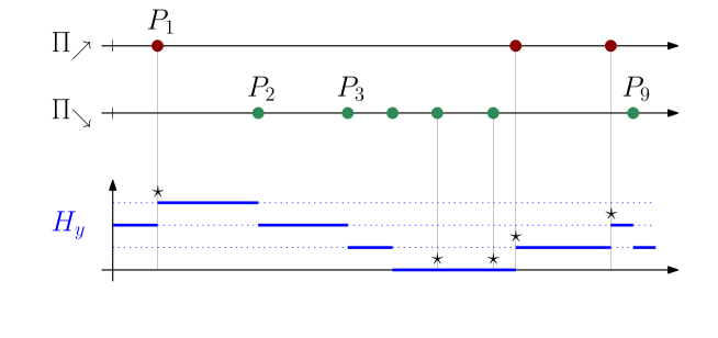
Figure 5: Notation of Lemma 18. Points of $\overline{\Pi}$ are depicted with $\star$’s.

Let $\Pi_{0}$ be the point process given by unused service times:

$$\Pi_{0}=\left\{y\in\Pi_{\searrow}\text{ such that }H_{y}=0\right\}.$$

Lemma 18.

The process $\overline{\Pi}:=\Pi_{\nearrow}\cup\Pi_{0}$ is a homogeneous PPP with intensity $\beta$.

Proof.

The point process $\Pi_{\nearrow}\cup\Pi_{\searrow}$ is a homogeneous PPP with intensity $\lambda+\beta$, independent from $H_{0}$. We claim that $\overline{\Pi}$ is a subset of $\Pi_{\nearrow}\cup\Pi_{\searrow}$ where each point in $\Pi_{\nearrow}\cup\Pi_{\searrow}$ is taken independently with probability $\beta/(\lambda+\beta)$, it is therefore a homogeneous PPP with intensity $\beta$.

We need a few notation in order to prove the claim. Set $P_{0}=0$ and for $i\geq 1$ let $P_{i}$ be the $i$-th point of $\Pi_{\nearrow}\cup\Pi_{\searrow}$ and let $(\tilde{H}_{i})_{i\geq 0}$ be the discrete-time embedded chain associated to $H$, i.e. $\tilde{H}_{i}=H_{P_{i}}$ for every $i$.

We will prove by induction that for every $i\geq 1$:

• the points $P_{i}$ belongs to $\tilde{\Pi}$ with probability $\beta/(\lambda+\beta)$ independently from the events $\{P_{1}\in\tilde{\Pi}\},\dots,\{P_{i-1}\in\tilde{\Pi}\}$;

• $\tilde{H}_{i}$ is independent from $\{P_{1}\in\tilde{\Pi}\},\dots,\{P_{i}\in\tilde{\Pi}\}$ and is a $\mathrm{Geometric}_{\geq 0}(1-\beta^{\star})$.

This implies the claim and proves the Lemma. For the base case:

$$\mathbb{P}(P_{1}\in\tilde{\Pi},\tilde{H}_{1}=k) =\mathbb{P}(P_{1}\in\Pi_{\nearrow},\tilde{H}_{0}=k-1)\mathbf{1}_{k\geq 1}+\mathbb{P}(P_{1}\in\Pi_{\searrow},\tilde{H}_{0}=0)\mathbf{1}_{k=0},$$

$$=\frac{\lambda}{\lambda+\beta}\times(1-\beta^{\star})(\beta^{\star})^{k-1}\mathbf{1}_{k\geq 1}+\frac{\beta}{\lambda+\beta}\times(1-\beta^{\star})\mathbf{1}_{k=0},$$

$$=\frac{\beta}{\lambda+\beta}\times(1-\beta^{\star})(\beta^{\star})^{k}\qquad\text{(recall $\beta\beta^{\star}=\lambda$).}$$

More generally let $E_{j}$ be one of the two events $P_{j}\in\tilde{\Pi}/P_{j}\notin\tilde{\Pi}$.

$$\mathbb{P}(P_{i}\in\tilde{\Pi},\tilde{H}_{i}=k\ |\ E_{1},\dots,E_{i-1})= \ \mathbb{P}(P_{i}\in\Pi_{\nearrow},\tilde{H}_{i-1}=k-1\ |\ E_{1},\dots,E_{i-1})\mathbf{1}_{k\geq 1}$$

$$+ \ \mathbb{P}(P_{i}\in\Pi_{\searrow},\tilde{H}_{i-1}=0\ |\ E_{1},\dots,E_{i-1})\mathbf{1}_{k=0},$$

$$= \ \mathbb{P}(P_{i}\in\Pi_{\nearrow},\tilde{H}_{i-1}=k-1)\mathbf{1}_{k\geq 1}$$

$$+ \ \mathbb{P}(P_{i}\in\Pi_{\searrow},\tilde{H}_{i-1}=0)\mathbf{1}_{k=0},\qquad\text{(by induction hypothesis).}$$

$$= \ \frac{\beta}{\lambda+\beta}\times(1-\beta^{\star})(\beta^{\star})^{k}.$$

∎

Acknowledgements.

This work started as a collaboration with Anne-Laure Basdevant, I would like to thank her very warmly. I am also extremely indebted to Valentin Féray for Lemma 14 and for having enlightened me on the links with [Bia01]. Finally, thanks to Sam Spiro for stimulating exchanges.

Lucas Gerin gerin@cmap.polytechnique.fr
Cmap, Cnrs, École Polytechnique,
Institut Polytechnique de Paris,
Route de Saclay,
91120 Palaiseau Cedex (France).

References

- [AD95] David Aldous and Persi Diaconis. Hammersley’s interacting particle process and longest increasing subsequences. Probability Theory and Related Fields, 103(2):199–213, 1995.
- [BDJ99] Jinho Baik, Percy Deift, and Kurt Johansson. On the distribution of the length of the longest increasing subsequence of random permutations. J. Amer. Math. Soc., 12(4):1119–1178, 1999.
- [BEGG16] Anne-Laure Basdevant, Nathanaël Enriquez, Lucas Gerin, and Jean-Baptiste Gouéré. Discrete Hammersley’s lines with sources and sinks. ALEA Lat. Am. J. Probab. Math. Stat., 13:33–52, 2016.
- [Bia01] Philippe Biane. Approximate factorization and concentration for characters of symmetric groups. Internat. Math. Res. Notices, (4):179–192, 2001.
- [Boy22] Alexandre Boyer. Chapter 3 (in English) of Stationnarité bidimensionnelle de modèles aléatoires du plan, 2022. PhD Thesis, available at https://tel.archives-ouvertes.fr/tel-03783603/.
- [CDH+22] Alexander Clifton, Bishal Deb, Yifeng Huang, Sam Spiro, and Semin Yoo. Continuously increasing subsequences of random multiset permutations. Sém. Lothar. Combin., 86B:Art. 4, 11, 2022. (Proceedings of FPSAC’22.).
- [CG05] Eric Cator and Piet Groeneboom. Hammersley’s process with sources and sinks. Annals of Probability, 33(3):879–903, 2005.
- [CG06] Eric Cator and Piet Groeneboom. Second class particles and cube root asymptotics for Hammersley’s process. Annals of Probability, 34(4):1273–1295, 2006.
- [CG19] Federico Ciech and Nicos Georgiou. Order of the variance in the discrete Hammersley process with boundaries. Journal of Statistical Physics, 176(3):591–638, 2019.
- [CLRS09] Thomas H. Cormen, Charles E. Leiserson, Ronald L. Rivest, and Clifford Stein. Introduction to algorithms. MIT Press, Cambridge, MA, third edition, 2009.
- [Fer96] Pablo A. Ferrari. Limit theorems for tagged particles. volume 2, pages 17–40. 1996. Disordered systems and statistical physics: rigorous results (Budapest, 1995).
- [FM06] Pablo A. Ferrari and J. B. Martin. Multi-class processes, dual points and queues. Markov Process. Related Fields, 12(2):175–201, 2006.
- [Ham72] John M. Hammersley. A few seedlings of research. In Proceedings of the 6th Berkeley Symp. Math. Statist. and Probability, volume 1, pages 345–394, 1972.
- [JŁR00] Svante Janson, Tomasz Łuczak, and Andrzej Rucinski. Random graphs. Wiley-Interscience Series in Discrete Mathematics and Optimization. Wiley-Interscience, New York, 2000.
- [Rom15] Dan Romik. The surprising mathematics of longest increasing subsequences, volume 4 of Institute of Mathematical Statistics Textbooks. Cambridge University Press, New York, 2015.
- [Sep97] Timo Seppäläinen. Increasing sequences of independent points on the planar lattice. Annals of Applied Probability, 7(4):886–898, 1997.
- [Ste97] John Michael Steele. Probability theory and combinatorial optimization. Society for Industrial and Applied Mathematics (SIAM), 1997.
- [VK77] Anatoly M. Veršik and Sergei V. Kerov. Asymptotics of Plancherel measure of symmetrical group and limit form of Young tables. Doklady Akademii Nauk SSSR, 233.6:1024–1027, 1977.
- [Wai19] Martin J. Wainwright. High-dimensional statistics, volume 48 of Cambridge Series in Statistical and Probabilistic Mathematics. Cambridge University Press, Cambridge, 2019.