The one step fixed-lag particle smoother
as a strategy to improve
the prediction step of particle filtering

Abstract

Sequential Monte Carlo methods have been a major advance in the field of numerical filtering for stochastic dynamical state-space systems with partial and noisy observations. However, these methods still have some weaknesses. One of its main weaknesses concerns the degeneracy of these particle filters due to the impoverishment of the particles. Indeed, during the prediction step of these filters, the particles explore the state space, and if this exploration phase is not done correctly, a large part of the particles will end up in areas that are weakly weighted by the new measurement and will be mostly eliminated. Only a few particles will remain, leading to a degeneracy of the filter. In order to improve this last step within the framework of the classic bootstrap particle filter, we propose a simple approximation of the one step fixed-lag smoother. At each time iteration, we propose to perform additional simulations during the prediction step in order to improve the likelihood of the selected particles. Note that we aim to propose an algorithm that is almost as fast and of the same order of complexity as the bootstrap particle filter, and which is robust in poorly conditioned filtering situations. We also investigate a robust version of this smoother.

1 Introduction

Since the 1980s sequential Monte Carlo (SMC) methods, also called particle filter (PF) methods [11, 6, 2, 7, 4], have met with vast success and broad usage in the context of nonlinear filtering for state-space models with partial and noisy observations, also known as hidden Markov models (HMM) for state-space models. The success of these methods is due to their ability to take into account, in a numerically realistic and efficient way, the non-linearity of the dynamics and the non-Gaussianity of the underlying conditional distributions.

The exact (i.e., non approximated) dynamics of these HMMs takes the form of a sequential Bayes formula represented in Eqs. (3)-(4) also called Bayesian filter. In the case of linear models with additive Gaussian noise, the Kalman filter gives an exact solution of this problem as well as an efficient algorithm to compute it. There are a few cases where this filter can be computed explicitly in a finite-dimensional way, but in the majority of cases it is necessary to use numerical approximation methods. Historically, the first method proposed is the extended Kalman filter (EKF) [1] and its variants, which consist in linearizing the model around the current estimate and applying the Kalman filter. But in the case of strongly nonlinear models, the EKF often diverges. Since the 1980s, Monte Carlo methods have become very effective alternatives, they are now recognized as a powerful tool in the estimation with Bayesian filters in nonlinear/non-Gaussian hidden Markov models.

Among Monte Carlo methods, the PF techniques rely on an online importance sampling approximation of the sequential Bayes formula (3)-(4). At each time iteration, the PF builds a set of particles i.e. an independently and identically distributed sample from an approximation of the theoretical solution of the Bayesian filter.

A PF time iteration classically includes two steps: a prediction step consisting in exploring the state space by moving the particles according to the state equation, followed by a correction step consisting in first weighting the particles according to their correspondence with the new observation, i.e. according to their likelihood, then resampling these particles according to their weight. These two steps can be understood respectively as the mutation and selection steps of genetic algorithms.

The first really efficient PF algorithm, namely the bootstrap particle filter (BPF) or sampling-importance-resampling filter proposed in 1993 [11], follows exactly these two steps.

The resampling step is essential, without it we notice after a few time iterations an impoverishment of the particles: very few particles, even one, will concentrate all the likelihood; the other particles then become useless, the filter then loses track of the current state.

This resampling step is therefore essential, but still it does not prevent another type of particle degeneracy [2, 21, 7, 27, 17]. The latter appears when the particles explore areas of the state space that are not in agreement with the new observation. This is due to the fact that in its classical version, especially in the case of BPF, the prediction step propagates the particles in the state space without taking into account the next observation. Thus, when we associate weights with particles using their value via the likelihood function, a large proportion of the particles may have almost zero weight, this phenomenon is aggravated by the machine epsilon. In the worst case, all the particles can have a zero weight, the filter has then completely lost track of the state evolution.

To overcome this problem it is relevant to take into account the observations in the prediction step consisting in exploring the state space. The auxiliary particle filter (APF) [23, 22] is one of the first attempts to take into account the observation in the prediction step. One can consult the review articles [9, 10] concerning the possibilities of improvement of particle filters.

Another possibility to overcome this difficulty, without using the observation following the current one, is to use robust versions of particle filters, such as the regime switching method [15] or the averaging-model approach [19, 25], which allow model uncertainties to be taken into account.

The present paper aims to propose a new PF algorithm, called predictive bootstrap particle smoother (PBPS), to further improve the prediction step but keeping the simplicity of the BPF. The principle of the PBPS is to take into account the current and the next observations for the prediction and correction steps. At each prediction step, we make additional explorations in order to better determine the likelihood according to the next observation. It can be seen as a simple approximation of the one step fixed-lag smoother. The additional explorations contribute to the correction step in order to improve the likelihood of the selected particles with the current and next observation.

We propose an algorithm that is only a little more complex than the BPF, which is why we do not consider more complex algorithms, like the smoother with a deeper time-lag. We also want to propose an efficient algorithm in case of unfavorable filtering situations such as when observability is poorly conditioned.

In Section 2 state-space models and the (exact) formulas for nonlinear filters and smoothers are presented. In Section 3, we first present the classical bootstrap particle filter (BPF), then the predictive bootstrap particle smoother (PBPS) and its “robustfied” version called regime switching predictive bootstrap particle smoother (RS-PBPS).

In Section 4 we present simulations in two test cases where observability is weakly conditioned. The first test case is a classical example in state space dimension 1 for which we compare the PBPS to the extended Kalman filter (EKF) [1], the unscented Kalman filter (UKF) [26, 13], the bootstrap particle filter (BPF) [11], and the the auxiliary particle filter (APF) [22]. The second is more realistic, it is a classical problem of bearing-only 2D tracking with a state space of dimension 4. In this case we first compare the PBPS to the BPF and the APF filters. In this example there are often model uncertainties, so it is relevant to use robust filters, and we compare the RS-PBPS to “robustified” versions of the particle filters.

2 Nonlinear filtering and smoothing

In order to simplify the presentation, we will make the abuse of notation, customary in this field, of representing probability distributions, e.g. $\mu({\textup{d}}x)$, by densities, e.g. $\mu(x)\,{\textup{d}}x$; we also represent the Dirac measure $\delta_{x_{0}}({\textup{d}}x)$ as $\delta_{x_{0}}(x)\,{\textup{d}}x$ where $\delta_{x_{0}}(x)$ is the Dirac function (with $\delta_{x_{0}}(x)=0$ if $x\neq x_{0}$, $\delta_{x_{0}}(x)=+\infty$ if $x=x_{0}$, and $\int\delta_{x_{0}}(x)\,{\textup{d}}x=1$).

2.1 The state space model

We consider a Markovian state-space model with state process $(X_{k})_{k\geq 0}$ taking values in $\mathbb{R}^{n}$ and observation process $(Y_{k})_{k\geq 1}$ taking values in $\mathbb{R}^{d}$. We suppose that conditionally on $(X_{k})_{k\geq 0}$, the observations $Y_{k}$ are independent.

The ingredients of the state-space model are:

$$q_{k}(x|x^{\prime}) \stackrel{{\scriptstyle\textup{\tiny def}}}{{=}}p_{X_{k}|X_{k-1}=x^{\prime}}(x)\,,$$ (state transition kernel)

$$\psi_{k,y}(x) \stackrel{{\scriptstyle\textup{\tiny def}}}{{=}}p_{Y_{k}|X_{k}=x}(y)\,,$$ (local likelihood function)

$$\rho_{0}(x) \stackrel{{\scriptstyle\textup{\tiny def}}}{{=}}p_{X_{0}}(x)\,,$$ (initial distribution)

for any $x,x^{\prime}\in\mathbb{R}^{n}$, $y\in\mathbb{R}^{d}$.

These ingredients can be made more explicit in the case of the following state space model:

$$X_{k} =f_{k-1}(X_{k-1})+g_{k-1}(X_{k-1})\,W_{k-1}\,,$$ (1)

$$Y_{k} =h_{k}(X_{k})+V_{k}\,,$$ (2)

for $k\geq 1$, where $X_{k}$ (resp. $Y_{k}$, $W_{k}$, $V_{k}$) takes values in $\mathbb{R}^{n}$ (resp. $\mathbb{R}^{d}$, $\mathbb{R}^{m}$, $\mathbb{R}^{d}$), $f_{k}$ (resp. $g_{k}$, $h_{k}$) is a differentiable and at most linear growth, uniformly in $k$, from $\mathbb{R}^{n}$ to $\mathbb{R}^{n}$ (resp. $\mathbb{R}^{d}$, $\mathbb{R}^{n\times m}$, $\mathbb{R}^{d}$), $g_{k}$ being also bounded. Random sequences $W_{k}$ and $V_{k}$ are independent centered white Gaussian noises with respective variances $R^{W}_{k}$ and $R^{V}_{k}$; $W_{k}$, $V_{k}$, $X_{0}$ being independent. In this case:

$$q_{k}(x|x^{\prime})=\frac{1}{\sqrt{(2\,\pi)^{n}\,\det R^{W}_{k-1}}}\times\\ \times\exp\Bigl{(}-\frac{1}{2}\bigl{[}x-f_{k-1}(x^{\prime})\bigr{]}^{*}\,\bigl{[}g_{k}(x^{\prime})\,R^{W}_{k-1}\,g_{k}(x^{\prime})^{*}\bigr{]}^{-1}\,\bigl{[}x-f_{k-1}(x^{\prime})\bigr{]}\Bigr{)}$$

and

$$\psi_{k,y}(x)\propto\exp\Bigl{(}-\frac{1}{2}\bigl{[}y-h_{k}(x)\bigr{]}^{*}\,[R^{V}_{k}]^{-1}\,\bigl{[}y-h_{k}(x)\bigr{]}\Bigr{)}$$

($\psi_{k,y}$ has to be known up to a multiplicative constant).

2.2 Nonlinear filtering

Nonlinear filtering aims at determining the conditional distribution $\eta_{k}$ of the current state $X_{k}$ given the past observations $Y_{1},\dots,Y_{k}$, namely:

$$\eta_{k}(x)\stackrel{{\scriptstyle\textup{\tiny def}}}{{=}}p_{X_{k}|Y_{1:k}=y_{1:k}}(x)\,,\ x\in\mathbb{R}^{n}$$

for any $k\geq 1$ and $y_{1:k}\in(\mathbb{R}^{d})^{k}$, here we use the notation:

“$$Y_{1:k} (Y_{1},\dots,Y_{k})$$” for

(e.g. $Y_{1:k}=y_{1:k}$ means $Y_{\ell}=y_{\ell}$ for all $\ell=1,\dots,k$).

The nonlinear filter allows us to determine $\eta_{k}$ from $\eta_{k-1}$ using the classical two-step recursive Bayes formula:

Prediction step. The predicted distribution $\eta_{k^{-}}(x)\stackrel{{\scriptstyle\textup{\tiny def}}}{{=}}p_{X_{k}|Y_{1:k-1}=y_{1:k-1}}(x)$ of $X_{k}$ given $Y_{1:k-1}=y_{1:k-1}$ is given by:

$$\eta_{k^{-}}(x)=\int_{\mathbb{R}^{n}}\ q_{k}(x|x^{\prime})\ \eta_{k-1}(x^{\prime})\ {\textup{d}}x^{\prime}\,,$$ (3)

for $x\in\mathbb{R}^{n}$.

Correction step. The new observation $Y_{k}=y_{k}$ allows the predicted distribution to be updated in order to obtain $\eta_{k}$ according to the Bayes formula:

$$\eta_{k}(x) =\frac{\psi_{k}(x)\,\eta_{k^{-}}(x)}{\int_{\mathbb{R}^{n}}\psi_{k}(x^{\prime})\,\eta_{k^{-}}(x^{\prime})\,{\textup{d}}x^{\prime}}\,,$$ (4)

for $x\in\mathbb{R}^{n}$; here and in order to simplify the notations, $\psi_{k}(x)$ represents $\psi_{k,y_{k}}(x)$.

Note that in the correction step (4) , $\eta_{k}$ is proportional to the product of $\eta_{k-1}$ and the local likelihood function, that is:

$$\eta_{k}(x)\propto\psi_{k}(x)\,\eta_{k^{-}}(x)\,.$$

2.3 Nonlinear smoothing

Define $\bar{\eta}_{k}(x)$ the conditional distribution of $X_{k}$ given $Y_{1:k+1}=y_{1:k+1}$, that is:

$$\bar{\eta}_{k}(x)\stackrel{{\scriptstyle\textup{\tiny def}}}{{=}}p_{X_{k}|Y_{1:k+1}=y_{1:k+1}}(x)\,,\ x\in\mathbb{R}^{n}$$

for any $k\geq 1$ and $y_{1:k+1}\in(\mathbb{R}^{d})^{k+1}$.

To get the recurrence equation for $\bar{\eta}_{k}(x)$, we consider the extended state vector $\mathbf{X}_{k}=(X_{k},X_{k-1})$, it’s a Markov with transition:

$$Q_{k}(x^{\prime},x^{\prime\prime}|x_{k-1},x_{k-2})=$$

$$\qquad=p_{X_{k},X_{k-1}|X_{k-1}=x_{k-1},X_{k-2}=x_{k-2}}(x^{\prime},x^{\prime\prime})$$

$$\qquad=p_{X_{k}|X_{k-1}=x^{\prime\prime},X_{k-1}=x_{k-1},X_{k-2}=x_{k-2}}(x^{\prime})\;p_{X_{k-1}|X_{k-1}=x_{k-1},X_{k-2}=x_{k-2}}(x^{\prime\prime})$$

$$\qquad=p_{X_{k}|X_{k-1}=x_{k-1},X_{k-2}=x_{k-2}}(x^{\prime})\;\delta_{x_{k-1}}(x^{\prime\prime})$$

$$\qquad=p_{X_{k}|X_{k-1}=x_{k-1}}(x^{\prime})\;\delta_{x_{k-1}}(x^{\prime\prime})$$

$$\qquad=q_{k}(x^{\prime}|x_{k-1})\;\delta_{x_{k-1}}(x^{\prime\prime})\,,$$

where $x^{\prime\prime}\to\delta_{x_{k-1}}(x^{\prime\prime})$ is the Dirac delta function in $x_{k-1}$ (here, we adopt the usual abuse of notation, which consists in representing the Dirac measure by the Dirac delta function: $\delta_{x}(x^{\prime})=0$ if $x^{\prime}\neq x$, $\delta_{x}(x^{\prime})=+\infty$ if $x^{\prime}=x$, and $\int\delta_{x}(x^{\prime})\,{\textup{d}}x^{\prime}=1$.)

The conditional distribution $\boldsymbol{\eta}_{k}(x^{\prime},x^{\prime\prime})$ of $\mathbf{X}_{k}=(X_{k},X_{k-1})$ given $Y_{1:k}=y_{1:k}$, we apply the previous filter formula:

$$\boldsymbol{\eta}_{k^{-}}(x^{\prime},x^{\prime\prime}) =\iint Q_{k}(x^{\prime},x^{\prime\prime}|x_{k-1},x_{k-2})\,\boldsymbol{\eta}_{k-1}(x_{k-1},x_{k-2})\,{\textup{d}}x_{k-1}\,{\textup{d}}x_{k-2}$$

$$=\iint q_{k}(x^{\prime}|x_{k-1})\,\delta_{x_{k-1}}(x^{\prime\prime})\,\boldsymbol{\eta}_{k-1}(x_{k-1},x_{k-2})\,{\textup{d}}x_{k-1}\,{\textup{d}}x_{k-2}$$

$$=\iint q_{k}(x^{\prime}|x_{k-1})\,\delta_{x_{k-1}}(x^{\prime\prime})\,\boldsymbol{\eta}_{k-1}(x^{\prime\prime},x_{k-2})\,{\textup{d}}x_{k-1}\,{\textup{d}}x_{k-2}\,,$$

and the distribution of $Y_{k}$ given $(X_{k}=x_{k},X_{k-1}=x_{k-1})$ is the distribution of $Y_{k}$ given $X_{k}=x_{k}$, hence:

$$\boldsymbol{\eta}_{k}(x^{\prime},x^{\prime\prime}) \propto\psi_{k}(x^{\prime})\,\boldsymbol{\eta}_{k^{-}}(x^{\prime},x^{\prime\prime})\,,$$ (5)

and the $x^{\prime\prime}$-marginal distribution of this last expression gives $\bar{\eta}_{k-1}(x^{\prime\prime})$, the conditional distribution of $X_{k-1}$ given $Y_{1:k}=y_{1:k}$.

2.4 Approximations

The main difficulty encountered by the nonlinear filter (3)-(4) lies in the two integrations. These integrations can be solved explicitly only in the linear/Gaussian case, leading to the Kalman filter, and in a very few other specific nonlinear/non-Gaussian cases. In the latter cases, the optimal filter can be solved explicitly in the form of a finite dimensional filter; hence in the vast majority of cases, it is necessary to use approximation techniques [4]. Among the approximation techniques, we will consider the extended Kalman filter (EKF) [1], the unscented Kalman filter (UKF) [26, 13] and particle filter techniques, also called sequential Monte Carlo techniques [11, 6], see [8] for a recent overview.

Concerning the particle filters, as we will see in the next section, it is important to notice that on the one hand we do not need to know the analytical expressions of the state transition kernel and of the initial distribution, we just need to be able to sample (efficiently) from them; on the other hand, we do need the analytical expression of the local likelihood function (up to a multiplicative constant), indeed, for a given $y$, we need to compute $\psi_{k,y}(x)$ for a very large number of $x$ values.

3 Particle approximations

Particle filtering, also known as sequential Monte Carlo (SMC) methods, is a set of computational techniques used for the approximation of nonlinear filters [6]. According to this approach, the nonlinear filter $\eta_{k}$ is approximated by $\eta_{k}^{N}$ of the form:

$$\eta_{k}^{N}(x) =\sum_{i=1}^{N}\omega^{i}_{k}\,\delta_{\xi_{k}^{i}}(x)\,,\ x\in\mathbb{R}^{n}\,.$$

composed of $N$ particles located in $\xi_{k}^{i}$ in $\mathbb{R}^{n}$ and associated weights $\omega^{i}_{k}$, the weights are positive and sum to one [6]. Ideally the particles are sampled from $\eta_{k}$ and the importance weight are all equal to $1/N$ (meaning that all the particles have the same “importance”).

Particle filters offer two essential advantages in numerical approximation:

• they are finite-dimensional filters in the sense that they are represented using a finite number of parameters, in this case the position of the particles (after selection), which can therefore be integrated into computer memory;

• the representation of particle filters, as weighted sums of Dirac measurements, greatly facilitates the calculation of integrals according to these filters; moreover, many operations can be parallelized as a function of the particle index (or vectorized with interpreted languages like Python).

In the 3 particle filters presented, at each time increment between two observations, in a first so-called “mutation” step, the particles explore the state space. A weight is then associated with each of these particles according to a fitness function (here a local likelihood function), these weights will be noted $\omega^{1:N}_{k}$ in the 3 cases, then in a second “selection” step, particules are selected based on the fact that particles with a high weight will have a greater probability of reproduction than particles with low weights (at constant number of particles $N$), leading to a family of particles noted $\xi^{1:N}_{k}$ in the 3 cases.

3.1 The bootstrap particle filter

The bootstrap particle filter (BPF) filter is a classical sequential importance resampling method: suppose we have a good approximation $\eta_{k-1}^{N}=\frac{1}{N}\sum_{i=1}^{N}\delta_{\xi_{k-1}^{i}}$ of $\eta_{k-1}$. We can apply the prediction step (3) to $\eta_{k-1}^{N}$ and get the following approximation of $\eta_{k^{-}}$:

$$\tilde{\eta}_{k^{-}}(x)\stackrel{{\scriptstyle\textup{\tiny def}}}{{=}}\int_{\mathbb{R}^{n}}\ q_{k}(x|x^{\prime})\ \eta_{k-1}^{N}(x^{\prime})\,{\textup{d}}x^{\prime}=\sum_{i=1}^{N}\omega_{k-1}^{i}\ q_{k}(x|\xi_{k-1}^{i})\,,$$

and then apply the correction step (4) and get the following approximation of $\eta_{k}$:

$$\tilde{\eta}_{k}(x)\stackrel{{\scriptstyle\textup{\tiny def}}}{{=}}\frac{\sum_{i=1}^{N}\omega_{k-1}^{i}\,\psi_{k}(x)\,q_{k}(x|\xi_{k-1}^{i})}{\int_{\mathbb{R}^{n}}\sum_{i=1}^{N}\omega_{k-1}^{i}\,\psi_{k}(x^{\prime})\,q_{k}(x^{\prime}|\xi_{k-1}^{i})\,{\textup{d}}x^{\prime}}\,,$$

but the two last approximations $\tilde{\eta}_{k^{-}}$ and $\tilde{\eta}_{k}$ are mixtures of the continuous densities $q_{k}(\,\cdot\,|\xi_{k-1}^{i})$ and therefore not of the particle type. The bootstrap particle filter (BPF) proposed by [11] is the simplest method to propose a particle approximation. For the prediction step we use the sampling technique:

$$\xi^{i}_{k^{-}}\sim q_{k}(\,\cdot\,|\xi^{i}_{k-1})\,,\ i=1:N\quad\,\textrm{(independently)}\,,$$

which is:

$$\xi^{i}_{k^{-}}=f_{k-1}(\xi^{i}_{k-1})+g_{k-1}(\xi^{i}_{k-1})\,\textrm{w}^{i}\,,$$

where $\textrm{w}^{i}$ are i.i.d. $N(0,R^{W}_{k-1})$ samples. Then we let

$$\eta_{k^{-}}^{N}(x)\stackrel{{\scriptstyle\textup{\tiny def}}}{{=}}\sum_{i=1}^{N}\omega_{k-1}^{i}\,\delta_{\xi_{k^{-}}^{i}}(x)\,.$$

Through the correction step (4), this approximation $\eta_{k^{-}}^{N}$ gives $\sum_{i=1}^{N}\omega_{k}^{i}\,\delta_{\xi_{k^{-}}^{i}}$ where:

$$\omega^{i}_{k}\stackrel{{\scriptstyle\textup{\tiny def}}}{{=}}\frac{\psi_{k}(\xi_{k^{-}}^{i})\,\omega_{k^{-}}^{i}}{\sum_{j=1}^{N}\psi_{k}(\xi_{k^{-}}^{j})\,\omega_{k^{-}}^{j}}$$ (6)

are the updated weights taking account of the new observation $y_{k}$ through the likelihood function $\psi_{k,y_{k}}$. This correction step must be completed by a resampling of the particles $\xi_{k^{-}}^{i}$ according to the importance weights $\omega^{i}_{k}$:

$$\xi_{k}^{i}\sim\sum_{j=1}^{N}\omega_{k}^{j}\,\delta_{\xi_{k^{-}}^{j}}\,,\ i=1:N\quad\textrm{(independently)}\,,$$ (7)

leading the to the particle approximation:

$$\eta_{k}^{N}(x)\stackrel{{\scriptstyle\textup{\tiny def}}}{{=}}\sum_{i=1}^{N}\omega_{k}^{i}\,\delta_{\xi_{k}^{i}}(x)\,,\ \textrm{with }\omega_{k}^{i}=\frac{1}{N}\,.$$

Algorithm 3.1 gives a summary of the BPF, in this version a resampling is performed at each time interval. The multinomial resampling step (7), whose basic idea is proposed in [11], could be greatly improved, there are several resampling techniques, see [5, 16] for more details.

1:  $\xi^{1:N}_{0}\mathrel{\mathop{\sim}\limits^{\vbox to0.27126pt{\kern-2.3pt\hbox{$\scriptstyle\textrm{\tiny iid}$}\vss}}}\rho_{0}$ # initialization

2:  return  $\xi_{0}^{1:N}$

3:  for $k=1,2,\dots$ do

4:     $\xi^{i}_{k^{-}}\sim q_{k}(\,\cdot\,|\xi^{i}_{k-1})\,,\ i=1:N$ # particles evolution

5:     $\omega^{i}_{k}\leftarrow\psi_{k}(\xi^{i}_{k^{-}})\,,\ i=1:N$ # likelihood

6:     $\omega^{i}_{k}\leftarrow{\omega^{i}_{k}}/{\sum_{j=1}^{N}\omega^{j}_{k}}\,,\ i=1:N$ # renormalization

7:     $\xi_{k}^{1:N}\mathrel{\mathop{\sim}\limits^{\vbox to0.27126pt{\kern-2.3pt\hbox{$\scriptstyle\textrm{\tiny iid}$}\vss}}}\sum_{j=1}^{N}\omega^{j}_{k}\,\delta_{\xi^{j}_{k^{-}}}$ # resampling

8:     return  $\xi_{k}^{1:N}$

9:  end for

Bootstrap particle filter (BPF).

It is not necessary to resample the particles systematically at each time iteration as in Algorithm 3.1. However, this resampling step should be done regularly in terms of time iterations to avoid degeneracy of the weights [6].

We will consider another degeneracy problem. Suppose that in step (6), the local likelihood values $\psi_{k}(\xi_{k^{-}}^{i})$ associated with the predicted particles $\xi_{k^{-}}^{i}$ are all very small, or even equal to zero due to rounding in floating point arithmetic. This normalization step (6) is then impossible. This problem occurs when the filter loses track of the true state $X_{k}$, i.e. the likelihood of the predicted particles $\xi_{k^{-}}^{i}$ w.r.t. the observation $y_{k}$ are all negligible, in this case the observation $y_{k}$ appears as an outlier. This occurs especially when the period of time between two successive instants of observation is very large compared to the dynamics of the state process. Strategies to overcome this weakness encompass the iterated extended Kalman particle filter [18] or the iterated unscented Kalman particle filter [12]; see [10] and [17] for reviews of the subject.

3.2 The predictive bootstrap particle smoother

The purpose of the predictive bootstrap filter (PBPS) is to improve the correction step (6) of the BPF by using both observations $Y_{k}=y_{k}$ and $Y_{k+1}=y_{k+1}$ at each iteration $k$. In a way, the PBPS can be seen as an approximation of the distribution of $X_{k}$ given $Y_{1:k+1}=y_{1:k+1}$, the one step fixed-lag smoother presented in Section 2.3.

In the proposed algorithm, the prediction step consists in a first step to propagate at time $k$ the $\eta_{k-1}^{N}$ particles by simulating the transition kernel sampler, then in a second step to extend these particles according to a one-step-ahead sampler. Then the correction step consists in updating the weights of the $N$ particles of $\eta_{k^{-}}^{N}$ according to their likelihood with $y_{k}$ and the likelihood of their one-step ahead offspring particles with $y_{k+1}$.

The iteration $k-1\to k$ of the filter is more precisely:

Prediction step.

As for the BPF we sample $N$ particles and compute $N$ normalized likelihood weights:

$$\tilde{\xi}^{i}_{k}\sim q_{k}(\,\cdot\,|\xi^{i}_{k-1})\,,\ \tilde{\omega}^{i}_{k}\propto\psi_{k}(\xi_{k^{-}}^{i})\,\omega_{k^{-}}^{i}\,,\ i=1:N\,.$$

Again we will resample the particles $\tilde{\xi}^{1:N}_{k}$, but instead of doing so according to the weights $\tilde{\omega}^{1:N}_{k}$, we will first modify the latter ones. For each index $i$, we generate a one-step-ahead offspring particles and compute its weight:

$$\tilde{\xi}^{i}_{k+1} \sim\tilde{q}_{k+1}(\,\cdot\,|\tilde{\xi}^{i}_{k})\,, \tilde{\omega}^{i}_{k+1} \stackrel{{\scriptstyle\textup{\tiny def}}}{{=}}\psi_{k+1}(\tilde{\xi}^{i}_{k+1}).$$

Note that the likelihood weights $\tilde{\omega}^{i}_{k+1}$ depend on the next observation $y_{k+1}$. The choice of the one-step-ahead sampler $\tilde{q}_{k+1}$ will be detailed at the end of this sub-section.

Correction step.

We compute the weights at time $k$ according to Eq. (5):

$$\omega^{i}_{k} \stackrel{{\scriptstyle\textup{\tiny def}}}{{=}}\tilde{\omega}^{i}_{k}\;\tilde{\omega}^{i}_{k+1}\qquad\textrm{for }i=1:N.$$

Then, $N$ particles $\tilde{\xi}^{1:N}_{k}$ are resampled according to the weights $\omega^{1:N}_{k}$.

The PBPS is depicted in Algorithm 3.2.

Choice of one-step-ahead sampler $\tilde{q}_{k+1}$

For the special case of the system (1)-(2) we can choose a simpler “deterministic sampler”:

$$\tilde{\xi}^{i}_{k+1}=f_{k}(\tilde{\xi}^{i}_{k})$$

which corresponds to the one-step-ahead mean:

$$\tilde{\xi}^{i}_{k+1} =\mathbb{E}\bigl{(}X_{k+1}\big{|}X_{k}=\tilde{\xi}^{i}_{k}\bigr{)}$$

$$=\mathbb{E}\bigl{(}f_{k}(X_{k})+g_{k}(X_{k})\,W_{k}\big{|}X_{k}=\tilde{\xi}^{i}_{k}\bigr{)}$$

$$=f_{k}(\tilde{\xi}^{i}_{k})+g_{k}(\tilde{\xi}^{i}_{k})\,\underbrace{\mathbb{E}(W_{k}|X_{k}=\tilde{\xi}^{i}_{k})}_{=0}=f_{k}(\tilde{\xi}^{i}_{k})\,.$$

This choice greatly reduces the computation burden and it is sufficient, as we will see, for a linear state equation. For a highly nonlinear state equation, we can choose $\tilde{q}_{k+1}=q_{k+1}$, which corresponds to a simulation of the state dynamic.

[t]

1:  $\xi^{1:N}_{0}\mathrel{\mathop{\sim}\limits^{\vbox to0.27126pt{\kern-2.3pt\hbox{$\scriptstyle\textrm{\tiny iid}$}\vss}}}\rho_{0}$ # initialization

2:  for $k=1,2,\dots$ do

3:     for $i=1:N$ do

4:        $\tilde{\xi}^{i}_{k}\sim q_{k}(\,\cdot\,|\xi^{i}_{k-1})$ # particles propagation

5:        $\tilde{\omega}^{i}_{k}\leftarrow\psi_{k}(\tilde{\xi}^{i}_{k})$

6:        $\tilde{\xi}^{i}_{k+1}=f_{k}(\tilde{\xi}^{i}_{k})$ # offspring

7:        $\tilde{\omega}^{i}_{k+1}\leftarrow\psi_{k+1}(\tilde{\xi}^{i}_{k+1})$ # offspring weighting

8:        $\omega^{i}_{k}\leftarrow\tilde{\omega}^{i}_{k}\,\tilde{\omega}^{i}_{k+1}$# particles weighting

9:     end for

10:     $\omega^{i}_{k}\leftarrow{\omega^{i}_{k}}/{\sum_{i^{\prime}=1}^{N}\omega^{i^{\prime}}_{k}}\,,\ i=1:N$ # weights normalization

11:     $\xi_{k}^{1:N}\mathrel{\mathop{\sim}\limits^{\vbox to0.27126pt{\kern-2.3pt\hbox{$\scriptstyle\textrm{\tiny iid}$}\vss}}}\sum_{i^{\prime}=1}^{N}\omega^{i^{\prime}}_{k}\,\delta_{\tilde{\xi}^{i^{\prime}}_{k}}$ # particles resampling

12:     return  $\xi_{k}^{1:N}$

13:  end for

predictive bootstrap particle smoother (PBPS).

3.3 The regime switching predictive bootstrap particle smoother

1:  $\xi^{1:N}_{0}\mathrel{\mathop{\sim}\limits^{\vbox to0.27126pt{\kern-2.3pt\hbox{$\scriptstyle\textrm{\tiny iid}$}\vss}}}\rho_{0}$ # initialization

2:  return  $\xi_{0}^{1:N}$

3:  for $k=1,2,\dots$ do

4:     $\mu^{1:N}_{k-1}\mathrel{\mathop{\sim}\limits^{\vbox to0.27126pt{\kern-2.3pt\hbox{$\scriptstyle\textrm{\tiny iid}$}\vss}}}U(\mathcal{M})$

5:     $\tilde{\xi}^{i}_{k}\sim q_{k}(\,\cdot\,|\xi^{i}_{k-1},\mu^{i}_{k-1})\,,\ i=1:N$ # particles propagation

6:     $\tilde{\omega}^{i}_{k}\leftarrow\psi_{k}(\tilde{\xi}^{i}_{k})\,,\ i=1:N$

7:     $\tilde{\xi}^{i}_{k+1}=f_{k}(\tilde{\xi}^{i}_{k})\,,\ i=1:N$ # offspring

8:     $\tilde{\omega}^{i}_{k+1}\leftarrow\psi_{k+1}(\tilde{\xi}^{i}_{k+1})\,,\ i=1:N$ # offspring weighting

9:     $\omega^{i}_{k}\leftarrow\tilde{\omega}^{i}_{k}\,\tilde{\omega}^{i}_{k+1}\,,\ i=1:N$ # particles weighting

10:     $\omega^{i}_{k}\leftarrow{\omega^{i}_{k}}/{\sum_{j=1}^{N}\omega^{j}_{k}}\,,\ i=1:N$ # renormalization

11:     $\xi_{k}^{1:N}\mathrel{\mathop{\sim}\limits^{\vbox to0.27126pt{\kern-2.3pt\hbox{$\scriptstyle\textrm{\tiny iid}$}\vss}}}\sum_{j=1}^{N}\omega^{j}_{k}\,\delta_{\tilde{\xi}^{j}_{k}}$ # resampling

12:     return  $\xi_{k}^{1:N}$

13:  end for

Regime Switching predictive bootstrap particle smoother (RS-PBPS)

In most applications, both the state model and the observation model are only partially known. As we will see in Section 4.2, applying a filter without care in such situations can be delicate. There are several techniques to make these filters more robust to model mismatch such as the dynamic model averaging (DMA) [19, 25] or the regime switching (RS) [15]. We will use both DMA and RS techniques in the simulations of Section 4.2, but we introduce only the RS technique in the present section by proposing a “robustified” version of PBPS, called regime switching PBPS (RS-PBPS).

The partial knowledge on the state-space model introduced in Section 2.1 can be related to the state model, i.e. to the the transition kernel $q_{k}$, or the observation model, i.e. the likelihood function $\psi_{k}$.

In the great majority of applications, the uncertainty relates to the state model, so we will restrict ourselves to this case. In order to model this uncertainty, we assume that the state dynamics corresponds to a transition kernel of the form:

$$q_{k}(x|x^{\prime},m)\,,$$

where $m$ is a parameter that evolves dynamically in the finite set:

$$\mathcal{M}=\{m_{1},\dots,m_{L}\}\,.$$

Thus $\mathcal{M}$ represents the different possible regimes of the state model over time.

The principle of these robust filters consists in making the particles and the weights evolve according to a mixture of the parameters $\mathcal{M}$. The dynamic model averaging particle filter (DMA-BPF) proposed in [25] is detailed in Algorithm Appendix: Algorithms, we will not describe it here.

We now present one of the algorithms proposed by [15]. We use the simplest of them which gives good results according to [15]. In the BPF, we replace the prediction step (Algorithm 3.1 line 4) by:

$$\mu^{1:N}_{k-1}\mathrel{\mathop{\sim}\limits^{\vbox to0.3014pt{\kern-2.3pt\hbox{$\scriptstyle\textrm{\tiny iid}$}\vss}}}U(\mathcal{M})\,,\quad\xi^{i}_{k}\sim q_{k}(\,\cdot\,|\xi^{i}_{k-1},\mu^{i}_{k-1})\,,\quad i=1:N\,,$$

where $U(\mathcal{M})$ is the uniform distribution on $\mathcal{M}$; the only difference lies in the fact that the particles are sampled at random according to the various models represented by $\mathcal{M}$. The resulting method called RS-BPF is described in Algorithm Appendix: Algorithms. The adaptation to PBPS and APF is also immediate, leading to the RS-PBPS and the RS-APF; the RS-PBPS is detailed in Algorithm 3.3.

4 Simulation studies

We compare numerically the PBPS to other filters on two space-state models where observability is weakly conditioned. The performance of the filters is compared using an empirical evaluation of the root-mean-square error (RMSE). We simulate $S$ independent trajectories $(X_{0:K}^{(s)},Y_{1:K}^{(s)})_{s=1:S}$ of the state-space models, where $K$ is the length of the chronological sequence of observations. For each simulation $s$, we ran $R$ times each filter $\mathcal{F}\in\{$BPF, PBPS, APF, DMA-BPF, RS-BPF, RS-APF, RS-PBPS$\}$ and we compute the root mean squared error at time $k$:

$$\textrm{RMSE}_{k}(\mathcal{F}) \stackrel{{\scriptstyle\textup{\tiny def}}}{{=}}\sqrt{\frac{1}{S}\sum_{s=1}^{S}\frac{1}{R}\sum_{r=1}^{R}\Bigl{|}\hat{X}^{\mathcal{F}(s,r)}_{k}-X^{(s)}_{k}\Bigr{|}^{2}}\,,$$ (8)

where:

$$\hat{X}_{k}^{\mathcal{F}(s,r)} \stackrel{{\scriptstyle\textup{\tiny def}}}{{=}}\int_{\mathbb{R}^{n}}x\,\eta_{k}^{N,\mathcal{F}(s,r)}(x)\,{\textup{d}}x=\frac{1}{N}\sum_{i=1}^{N}\xi_{k}^{\mathcal{F}(s,r),i}$$

is the numerical approximation of $\hat{X}^{(s)}_{k}=\mathbb{E}(X^{(s)}_{k}|Y^{(s)}_{1:k})$ by the filter $\mathcal{F}$. We also compute the global root mean squared error:

$$\textrm{RMSE}(\mathcal{F}) \stackrel{{\scriptstyle\textup{\tiny def}}}{{=}}\frac{1}{K}\sum_{k=1}^{K}\textrm{RMSE}_{k}(\mathcal{F})\,.$$

Note that for the EKF and UKF filters the summation over $r$ in (8) is useless.

All implementations are done in R language [24] using a 2.11 GHz core i7-8650U intel running Windows 10 64bits with a 16 Go RAM.

4.1 First case study: a one-dimensional model

We consider the following one-dimensional nonlinear model [11, 14, 6]:

$$\begin{split}X_{k}&=\frac{X_{k-1}}{2}+\frac{25\,X_{k-1}}{1+X_{k-1}^{2}}+8\cos\bigl{(}1.2\,(k-1)\bigr{)}+W_{k-1}\,,\\ Y_{k}&=\frac{X_{k}^{2}}{20}+V_{k}\,,\end{split}$$ (9)

with $1\leq k\leq K$ ($K=50$), $X_{0}\sim\mathcal{N}(0,1)$; $W_{k}\mathrel{\mathop{\sim}\limits^{\vbox to0.3014pt{\kern-2.3pt\hbox{$\scriptstyle\textrm{\tiny iid}$}\vss}}}\mathcal{N}(0,3^{2})$, $V_{k}\mathrel{\mathop{\sim}\limits^{\vbox to0.3014pt{\kern-2.3pt\hbox{$\scriptstyle\textrm{\tiny iid}$}\vss}}}\mathcal{N}(0,1)$; $X_{0}$, $(W_{k})_{k\geq 1}$ and $(V_{k})_{k\geq 1}$ mutually independent. Note that the state process $X_{k}$ is observed only through $X_{k}^{2}$ so the filters have difficulties in determining whether $X_{k}$ is positive or negative, especially since the state process $X_{k}$ regularly changes it’s sign. Thus this model is regularly used as benchmark for testing filters, as filters may easily lose track of $X_{k}$.

For this example we compare the filters PBPS, BPF, APF, EKF and UKF.

In Figure 1 we plot, as a function of different values of $N$ (50, 100, 500, 1000, 3000, 5000), on the left the average computation time for the filtering a trajectory, and on the right the RMSE (with $S=100$, $R=40$).

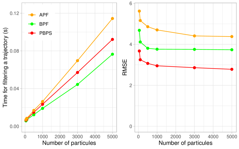
Figure 1: One-dimensional case study (9) — We plot the average computation time for filtering a trajectory (left) and the RMSE (right) of the filters PBPS, BPF and APF as a function of different values of $N$ (50, 100, 500, 1000, 3000, 5000) (with $S=100$ and $R=40$). In comparison, the EKF and UKF have a respective RMSE of 16.83 and 6.88 (and a negligible computation time compared to the particle approximations).

The computation times of EKF and UKF are negligible compared to those of the particle approximations. On the other hand, the RMSE of EKF (16.83) are much higher than those of the particle approximations; UKF with an RMSE of 6.88 behaves much better than EKF but is still less accurate than the particle approximations.

The computation time of PBPS is naturally higher than that of BPF, but the latter is much less accurate. For example, PBPS with $N=50$ particles is 15 times faster than BPF with $N=5000$ particles while being 30% more accurate.

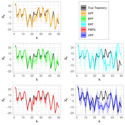
Figure 2: One-dimensional case study (9) — On a single simulation, for each filter, we plot the true state trajectory $k\to X_{k}$ and the approximation $k\to\hat{X}_{k}$ with the associated $95\%$ confidence region ($N=5000$).

In Figure 2, for each filter $\mathcal{F}\in\{\textrm{PBPS, BPF, APF, EKF, UKF}\}$ (with $N=5000$), we plot the true state trajectory $k\to X_{k}$, the approximation $k\to\hat{X}^{\mathcal{F}}_{k}$, and the associated 95% confidence regions. For the particle approximations the confidence interval is given empirically by the particles, for the EKF and UKF it is given as an approximated Gaussian confidence interval. The PBPS approximation has a smaller error $k\to|\hat{X}^{\mathcal{F}}_{k}-X_{k}|$ and a smaller confidence region than the other filters.

In Figure 3, we compare $k\to\textrm{RMSE}_{k}(\mathcal{F})$ for $\mathcal{F}\in\{$PBPS, BPF, APF, EKF, UKF$\}$ (with $N=5000$). Again, we see that the PBPS behaves better than the other filters and that the EKF has a very erratic behavior.

The poor behavior of the EKF can be explained by the very nonlinear nature of this example and by the observability problem around 0. Note the relatively good behavior of the UKF. However, because of the observability problem at 0, both the UKF and the EKF cannot find the track of $X_{k}$ once in the wrong half-plane (Figure 2 around time $k=30$).

In Figure 4, in the case of a single simulation of the state-space system and of the BPF and PBPS filters (with $N=5000$), we plot the true trajectory $k\to X_{k}$ as well as the set of particles $k\to\xi_{k}^{\mathcal{F},1:N}$ for $\mathcal{F}\in\{$BPF, PBPS$\}$. Not surprisingly, we find that the PBPS particles are more concentrated around the true value $X_{k}$ and that BPF more often “loads” the symmetric part of the state space. Indeed, the smoothing allows us to reduce the variance but also to compensate the observability ambiguities; it is for this purpose that it was designed, and we reiterate that this gain is obtained with a great improvement in the computation time (provided that less particles are used).

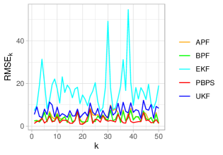
Figure 3: One-dimensional case study (9) — We compare $k\to\textrm{RMSE}_{k}$ for each filter ($S=100$, $R=40$, $N=5000$).

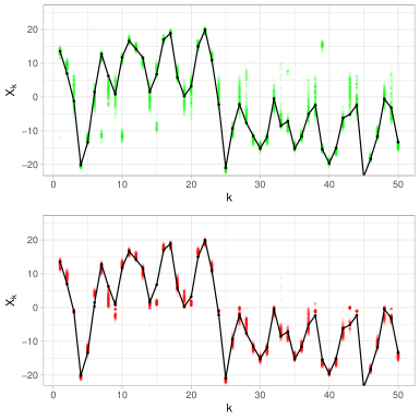
Figure 4: One-dimensional case study (9) — On a single simulation, we plot the true value $k\to X_{k}$ with the evolution of the set of $N=500$ particles $k\to\xi^{1:N}_{k}$ for the BPF (top) and the PBPS (bottom); the particles are represented in transparency to better reflect their density.

4.2 Second case study: a four-dimensional bearings-only tracking model

We consider the following four-dimensional model [11, 23, 3]:

$$\begin{split}X_{k}&=\left(\begin{smallmatrix}1&0&1&0\\ 0&1&0&1\\ 0&0&1&0\\ 0&0&0&1\end{smallmatrix}\right)\,X_{k-1}+\sigma_{W}\,\left(\begin{smallmatrix}0.5&0\\ 0&0.5\\ 1&0\\ 0&1\\ \end{smallmatrix}\right)\,W_{k-1}\,,\\ Y_{k}&\sim\textrm{wrapped Cauchy}\Bigl{(}\arctan\Bigl{(}\frac{X_{k}[1]}{X_{k}[2]}\Bigr{)},\rho\Bigr{)},\end{split}$$ (10)

with $1\leq k\leq K=20$, $X_{0}\sim\mathcal{N}(\bar{X}_{0},P_{0})$ with:

$$\bar{X}_{0}=\bigl{(}-0.05,0.2,0.001,-0.055\bigr{)}^{*}\,,$$

$$P_{0}=0.01\,\textrm{diag}\bigl{(}0.5^{2},0.3^{2},0.005^{2},0.01^{2}\bigr{)}\,,$$

$\sigma_{W}=0.001$, $W_{k}\mathrel{\mathop{\sim}\limits^{\vbox to0.3014pt{\kern-2.3pt\hbox{$\scriptstyle\textrm{\tiny iid}$}\vss}}}\mathcal{N}(0,I_{2\times 2})$, $\rho=1-0.005^{2}$, $X_{0}$ and $(W_{k})_{k\geq 1}$ mutually independent; conditionally on $(X_{k})_{k\geq 0}$, $(Y_{k})_{k\geq 1}$ and $(W_{k})_{k\geq 1}$ are independent.

The state equation corresponds to a target moving on a plane. The state vector is:

$$X_{k}=(X_{k}[1],X_{k}[2],X_{k}[3],X_{k}[4])^{*}=(x_{1},x_{2},\dot{x}_{1},\dot{x}_{2})^{*}\,,$$

where $(x_{1},x_{2})$ are the Cartesian coordinates of the target in the plane and $(\dot{x}_{1},\dot{x}_{2})$ are the corresponding velocities. The observer is located at the origin of the plane and accessed only to the azimuth angle $\beta=\arctan(x_{1}/x_{2})\in[-\pi,\pi]$ corrupted by noise.

It is known that in the situation where the observer follows a rectilinear trajectory at constant speed, or zero speed as here, the filtering problem is poorly conditioned [20]. This is a situation where it is known for example that the EKF diverges very strongly.

The conditional probability density function of the measured angle $Y_{k}$ given the state $X_{k}$ is assumed to be a wrapped Cauchy distribution with concentration parameter $\rho$ [23]:

$$p_{Y_{k}|X_{k}=x}(y)=\frac{(2\,\pi)^{-1}\,(1-\rho^{2})}{1+\rho^{2}-2\,\rho\,\cos\Bigl{(}y-\arctan(\frac{x[1]}{x[2]}))\Bigr{)}}$$ (11)

for $-\pi\leq y<\pi$, where $\rho\in[0,1]$ is the mean resultant length. Note that the state dynamics is linear and Gaussian, but the observation dynamics is nonlinear and non-Gaussian.

Classically, in tracking studies, the trajectory model (the state equation) does not correspond to reality. In reality, the target follows a uniform straight trajectory sometimes interrupted by changes in heading and/or speed. The variance $\sigma_{W}$ of the state equation (10) appears then as a parameter of the filter: if it is too small, the filter will have trouble tracking the target, if it is too large, the particles will spread out too much, the filter will then lose accuracy, and even lose track of the target.

For bearings-only tracking applications, the EKF and UKF filters have poor performances and will therefore not be considered in this example. On the other hand, the robust filters introduced in Section 3.3 are relevant here because there is a mismatch model.

We compare the filters in two scenarios (with $K=40$ time steps):

• the target follows a uniform rectilinear motion;

• the target follows a uniform rectilinear motion with a change of heading at the middle of the simulation.

As we will see, the first scenario is simpler than the second. For the filter we consider two different values for $\sigma_{W}$: a small value $\sigma_{W}=0.001$ and a large $\sigma_{W}=0.003$. $\sigma_{W}=0.001$ is in fact too small to be consistent with the simulated trajectory, the second value $\sigma_{W}=0.003$ is more consistent with the simulated trajectory. For the robust filter we consider:

$$\mathcal{M}=\{0.0005,\,0.001,\,0.003,\,0.005\}$$

as the set of possible models.

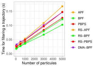
Figure 5: Four-dimensional case study (11) — We plot the average computation time for filtering a trajectory of the filters PBPS, BPF, APF, RS-PBPS, RS-BPF, RS-APF and DMA-BPF as a function of different values of $N$ (50, 100, 500, 1000, 3000, 5000) (with $S=20$ and $R=50$).

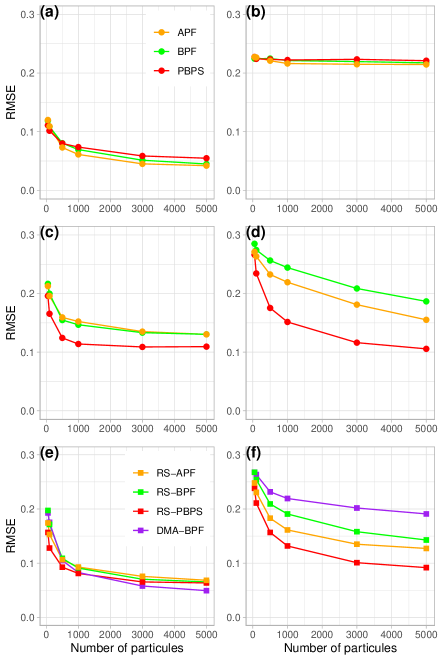
Figure 6: Four-dimensional case study (11) — Evolution of the RMSE as a function of the number $N$ of particles: the left column corresponds to the case without a turn, the right column to the case with a turn. For PBPS, BPF and APF, the first row (top) presents the RMSE for with $\sigma_{W}=0.001$, the second (middle) with $\sigma_{W}=0.003$. The third row (bottom) shows the RMSE for the RS-PBPS, RS-BPF, RS-APF, and DMA-BPF filters.

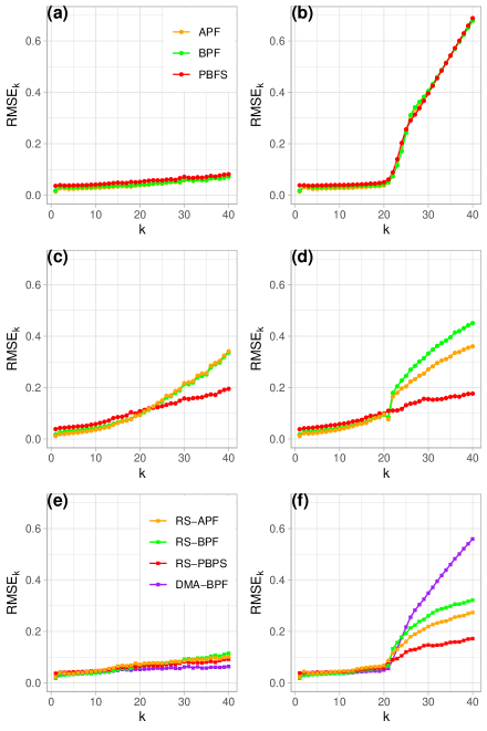
Figure 7: Four-dimensional case study (11) — $k\to$RMSE_k (for $N=5000$, $R=50$, $S=20$) for the different filters: the left column corresponds to the case without a turn, the right column to the case with a turn; PBPS, BPF and APF for with $\sigma_{W}=0.001$, on the first row; PBPS, BPF and APF for with $\sigma_{W}=0.003$, on the middle row; RS-PBPS, RS-BPF, RS-APF, and DMA-BPF, on the bottom row.

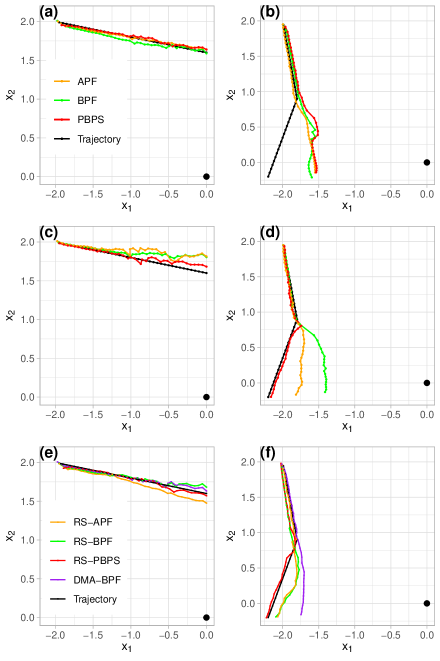
Figure 8: Four-dimensional case study (11) — On a single simulation and for each filter, we plot the true trajectory of the target with the estimates of each filter: without turn in the left column, with 1 turn in the right column; PBPS, BPS and APF filters with small $\sigma_{W}=0.001$ in the top row, PBPS, BPS and APF filters with large $\sigma_{W}=0.003$ in the middle row, RS-PBPS, RS-BPS, RS-APF, and DMA-BPF filters in the bottom row. The observer is in position $(0,0)$.

In Figure 5 we present the average computation times for filtering a trajectory as a function of different values of $N$ (50, 100, 500, 1000, 3000, 5000) (with $S=20$ and $R=50$).

In Figure 6, in agreement with Figure 5, we present the evolution of the RMSE as a function of the number $N$ of particles: the left column corresponds to the case without a turn, the right column to the case with a turn. For PBPS, BPF and APF, the first row (top) presents the RMSE for with $\sigma_{W}=0.001$, the second (middle) with $\sigma_{W}=0.003$. The third row (bottom) shows the RMSE for the RS-PBPS, RS-BPF, RS-APF, and DMA-BPF filters.

In Figure 7 we plot $k\to\$RMSE_k (for $N=5000$, $R=50$, $S=20$) for the different filters: the left column corresponds to the case without a turn, the right column to the case with a turn; PBPS, BPF and APF for with $\sigma_{W}=0.001$, on the first row; PBPS, BPF and APF for with $\sigma_{W}=0.003$, on the middle row; RS-PBPS, RS-BPF, RS-APF, and DMA-BPF, on the bottom row.

In Figure 8, on a single simulation and for each filter, we plot the true trajectory of the target with the estimates of each filter: without turn in the left column, with 1 turn in the right column; PBPS, BPS and APF filters with small $\sigma_{W}=0.001$ in the top row, PBPS, BPS and APF filters with large $\sigma_{W}=0.003$ in the middle row, RS-PBPS, RS-BPS, RS-APF, and DMA-BPF filters in the bottom row.

According to Figure 5, at the same number of particles, BPF is slightly faster than PBPS, both being faster than APF. The overheads for the robust version (RS) are also reasonable. In terms of complexity, the computation time is linear with the number of particles.

In order to better understand the situation, we will first comment on Figures 7 and 8: with a too small $\sigma_{W}$, the filters are able to track the target when it stays in a straight line (a) but they are not able to adapt when a turn occurs and continue the tracking more or less in a straight line (b). With a larger $\sigma_{W}$, the filters are still able to track the target when it remains in a straight line (c) with a small and increasing inaccuracy; in contrast only PBPS behaves reasonably well when a turn occurs (d). Except DMA-BPF which has a bad behavior, the RS robust filters behave better and RS-PBPS remains better than all the others (e) and (f).

From Figures 5 and 6, in the case of a turn, which is the most complex situation, we see that in order to reach PBPS/RS-PBPS accuracy with $N=1000$ the other filters must use $N=5000$ particles, and even in this case PBPS/RS-PBPS is at least twice as fast as the others.

5 Discussion and conclusion

In this paper, our aim was to propose a particle approximation method, not much more complex than the boostrap particle filter, which reduces the error variance, while being more robust in weakly conditioned situations, especially when observability conditions are poor.

We have therefore proposed an new particle filter algorithm, called predictive bootstrap particle smoother (PBPS), that deviates slightly from the strict filtering method in the sense that it takes into account the next observation in addition to the current one. We can thus consider PBPS as an approximation of the smoother with a fixed-lag interval of one step. However, the proposed algorithm is considerably simpler than the smoothing algorithms.

Furthermore, a way of making a filter more robust is to extend it to a “regime switching” strategy framework as proposed in [15]; which is what we have done by proposing a robustified version of PBPS.

In the considered examples, EKF shows very poor performance, which is perfectly understandable due to the very nonlinear nature and the poor observability conditions of the examples. It should be noted that UKF performs much better than EKF while remaining far from the performance of particle filters. Among the particle filters, APF performs slightly less well than than PBF and PBPS. Finally, even if for a given number of particles, BPF is faster than PBPS, the latter presents both a lower error variance and a much better behavior regarding observability problems. In terms of accuracy, PBPS with 1000 particles is still better than BPF with 5000 particles while being much faster. This is also the case when comparing RS-PBPS with RS-BPF

These performances are due to the fact that PBPS is a very simplified approximation of the one time step fixed-lag smoother. A strategy using a deeper fixed-lag interval of 2 or more time steps would be too costly and would not allow us to recover such performances.

In view of the performance of PBPS it would be interesting to develop strategies where the number $N$ of particles adapts dynamically to the problem conditions. It would also be interesting to test the PBPS strategy in other cases, such as when the time between two consecutive observations is important and requires several successive prediction steps.

Appendix: Algorithms

[H]

1:  $\xi^{1:N}_{0}\mathrel{\mathop{\sim}\limits^{\vbox to0.24112pt{\kern-2.3pt\hbox{$\scriptstyle\textrm{\tiny iid}$}\vss}}}\rho_{0}$ # initialization

2:  return  $\xi_{0}^{1:N}$

3:  for $k=1:K$ do

4:     $\bar{\xi}^{i}_{k}=\mathbb{E}(X_{k}|X_{k-1}=\xi^{i}_{k-1})\,,\ i=1:N$ # mean particle evolution

5:     $\bar{\omega}_{k}^{i}\leftarrow\psi_{k}(\bar{\xi}^{i}_{k})\,,\ i=1:N$ # ... and weighting

6:     $\tilde{\xi}_{k-1}^{1:N}\mathrel{\mathop{\sim}\limits^{\vbox to0.24112pt{\kern-2.3pt\hbox{$\scriptstyle\textrm{\tiny iid}$}\vss}}}\sum_{j=1}^{N}\bar{\omega}_{k}^{i}\,\delta_{\xi^{j}_{k-1}}$ # initial particles resampling

7:     $\xi^{i}_{k^{-}}\sim q_{k}(\,\cdot\,|\tilde{\xi}^{i}_{k-1})\,,\ i=1:N$ # particles propagation

8:     $\omega^{i}_{k}\leftarrow\psi_{k}(\xi^{i}_{k^{-}})/\bar{\omega}_{k}^{i}\,,\ i=1:N$ # likelihood

9:     $\omega^{i}_{k}\leftarrow{\omega^{i}_{k}}/{\sum_{j=1}^{N}\omega^{j}_{k}}\,,\ i=1:N$ # renormalization

10:     $\xi_{k}^{1:N}\mathrel{\mathop{\sim}\limits^{\vbox to0.24112pt{\kern-2.3pt\hbox{$\scriptstyle\textrm{\tiny iid}$}\vss}}}\sum_{j=1}^{N}\omega^{j}_{k}\,\delta_{\xi^{j}_{k^{-}}}$ # resampling

11:     return  $\xi_{k}^{1:N}$

12:  end for

Auxiliary particle filter (APF). Note that in the case of the (1)-(2), the first step, line 4, is reduced to $\bar{\xi}^{i}_{k}=\mathbb{E}(X_{k}|X_{k-1}=\xi^{i}_{k-1})=f_{k-1}(\xi^{i}_{k-1})$

[H]

1:  $\xi^{1:N}_{0}\mathrel{\mathop{\sim}\limits^{\vbox to0.24112pt{\kern-2.3pt\hbox{$\scriptstyle\textrm{\tiny iid}$}\vss}}}\rho_{0}$, $\mu^{1:N}_{0}\mathrel{\mathop{\sim}\limits^{\vbox to0.24112pt{\kern-2.3pt\hbox{$\scriptstyle\textrm{\tiny iid}$}\vss}}}U(\mathcal{M})$ # initialization

2:  return  $\xi_{0}^{1:N}$

3:  for $k=1:K$ do

4:     $\xi^{i}_{k^{*}}\sim q_{k}(\,\cdot\,|\xi^{i}_{k-1},\mu^{i}_{k-1})$, $i=1:N$

5:     $\omega^{l}_{k}=\sum_{i=1}^{N}\psi_{k}(\xi^{i}_{k^{*}}){\mathrm{\mathbf{missing}}1}_{\mu^{i}_{k-1}=m_{l}}$, $l=1:L$ # likelihood of candidate models

6:     $N_{k}^{1:L}\mathrel{\mathop{\sim}\limits^{\vbox to0.24112pt{\kern-2.3pt\hbox{$\scriptstyle\textrm{\tiny iid}$}\vss}}}\textrm{Multinomial}(N;m_{1},\dots,m_{L};\omega^{1}_{k},\cdots,\omega^{L}_{k})$with $N_{k}^{1}+\dots+N_{k}^{L}=N$ # number of particles per candidate model

7:     $\hat{\xi}^{1,1:L}_{k-1}\mathrel{\mathop{\sim}\limits^{\vbox to0.24112pt{\kern-2.3pt\hbox{$\scriptstyle\textrm{\tiny iid}$}\vss}}}\sum_{j=1}^{N}\delta_{\xi^{j}_{k-1}}\,\delta_{\mu^{j}_{k-1}=m_{l}}$ # initial particles resampling dgg # per candidate model

8:     $(\tilde{\xi}_{k-1}^{1:N},\mu_{k}^{1:N})\leftarrow(\hat{\xi}^{1:N_{k}^{1},1}_{k-1},m_{1}),(\hat{\xi}^{1:N_{k}^{2},2}_{k-1},m_{2}),\dots,(\hat{\xi}^{1:N_{k}^{L},L}_{k-1},m_{L})$

9:     $\xi^{i}_{k}\sim q_{k}(\,\cdot\,|\tilde{\xi}^{i}_{k-1},\mu^{i}_{k})\,,\ i=1:N$ # particles propagation

10:     return  $\xi_{k}^{1:N}$

11:  end for

Dynamic model averaging bootstrap particle filter (DMA-BPF) [25].

[H]

1:  $\xi^{1:N}_{0}\mathrel{\mathop{\sim}\limits^{\vbox to0.24112pt{\kern-2.3pt\hbox{$\scriptstyle\textrm{\tiny iid}$}\vss}}}\rho_{0}$ # initialization

2:  return  $\xi_{0}^{1:N}$

3:  for $k=1:K$ do

4:     $\mu^{1:N}_{k-1}\mathrel{\mathop{\sim}\limits^{\vbox to0.24112pt{\kern-2.3pt\hbox{$\scriptstyle\textrm{\tiny iid}$}\vss}}}U(\mathcal{M})$

5:     $\xi^{i}_{k^{-}}\sim q_{k}(\,\cdot\,|\xi^{i}_{k-1},\mu^{i}_{k-1})$, $i=1:N$ # particles propagation

6:     $\omega^{i}_{k}\leftarrow\psi_{k}(\xi^{i}_{k^{-}})\,,\ i=1:N$ # likelihood

7:     $\omega^{i}_{k}\leftarrow{\omega^{i}_{k}}/{\sum_{j=1}^{N}\omega^{j}_{k}}$, $i=1:N$ # renormalization

8:     $\xi_{k}^{1:N}\mathrel{\mathop{\sim}\limits^{\vbox to0.24112pt{\kern-2.3pt\hbox{$\scriptstyle\textrm{\tiny iid}$}\vss}}}\sum_{j=1}^{N}\omega^{j}_{k}\,\delta_{\xi^{j}_{k^{-}}}$ # resampling

9:     return  $\xi_{k}^{1:N}$

10:  end for

Regime Switching Bootstrap Particle Filter (RS-BPF) [15].

References

- [1] B.. Anderson and J.. Moore “Optimal Filtering” Prentice-Hall, 1979
- [2] M.. Arulampalam, S. Maskell, N. Gordon and T. Clapp “A tutorial on particle filters for online nonlinear/non-Gaussian Bayesian tracking” In IEEE Transactions on Signal Processing 50.2 Institute of ElectricalElectronics Engineers (IEEE), 2002, pp. 174–188 DOI: 10.1109/78.978374
- [3] F. Campillo and V. Rossi “Convolution particle filter for parameter estimation in general state-space models” In IEEE Transactions on Aerospace and Electronic Systems 45.3 Institute of ElectricalElectronics Engineers (IEEE), 2009, pp. 1063–1072 DOI: 10.1109/taes.2009.5259183
- [4] “The Oxford Handbook of Nonlinear Filtering” Oxford University Press, 2011 URL: https://global.oup.com/academic/product/the-oxford-handbook-of-nonlinear-filtering-9780199532902?cc=fr&lang=en&
- [5] R. Douc and O. Cappé “Comparison of resampling schemes for particle filtering” In Proceedings of the 4th International Symposium on Image and Signal Processing and Analysis, ISPA, 2005
- [6] “Sequential Monte Carlo Methods in Practice” Springer New York, 2001 DOI: https://doi.org/10.1007/978-1-4757-3437-9
- [7] A. Doucet and A.. Johansen “A Tutorial on Particle Filtering and Smoothing: Fifteen years later” In [4], 2011
- [8] A. Doucet and A. Lee “Sequential Monte Carlo Methods” In Handbook of Graphical Models Chapman & Hall/CRC, 2018
- [9] S. Godsill “Particle Filtering: the First 25 Years and beyond” In ICASSP 2019 - 2019 IEEE International Conference on Acoustics, Speech and Signal Processing (ICASSP) IEEE, 2019, pp. 7760–7764 DOI: 10.1109/icassp.2019.8683411
- [10] S.. Godsill and T. Clapp “Improvement strategies for Monte Carlo particle filters” In [6], 2001, pp. 139–158
- [11] N.. Gordon, D.. Salmond and A… Smith “Novel approach to nonlinear/non–Gaussian Bayesian state estimation” In IEEE Proceedings F Radar and Signal Processing 140.2, 1993, pp. 107–113 DOI: 10.1049/IP-F-2.1993.0015
- [12] W. Guo, C. Han and M. Lei “Improved unscented particle filter for nonlinear Bayesian estimation” In 10th International Conference on Information Fusion, 2007 DOI: 10.1109/ICIF.2007.4407986
- [13] S.. Julier and J.. Uhlmann “Unscented Filtering and Nonlinear Estimation” In IEEE Review 92.3 Institute of ElectricalElectronics Engineers (IEEE), 2004, pp. 401–422 DOI: 10.1109/jproc.2003.823141
- [14] G. Kitagawa “Monte Carlo filter and smoother for non-Gaussian nonlinear state space models” In Journal of Computational and Graphical Statistics 5.1 Informa UK Limited, 1996, pp. 1–25 DOI: https://doi.org/10.2307/1390750
- [15] Y. El-Laham, L. Yang, P.. Djurić and M.. Bugallo “Particle Filtering Under General Regime Switching” In 2020 28th European Signal Processing Conference (EUSIPCO), 2021, pp. 2378–2382 DOI: 10.23919/Eusipco47968.2020.9287507
- [16] T. Li, M. Bolic and P.. Djuric “Resampling Methods for Particle Filtering: Classification, implementation, and strategies” In IEEE Signal Processing Magazine 32.3, 2015, pp. 70–86 DOI: 10.1109/MSP.2014.2330626
- [17] T. Li, S. Sun, T.. Sattar and J.. Corchado “Fight sample degeneracy and impoverishment in particle filters: A review of intelligent approaches” In Expert Systems with Applications 41.8, 2014, pp. 3944–3954 DOI: https://doi.org/10.1016/j.eswa.2013.12.031
- [18] L. Liang-Qun, J. Hong-Bing and L. Jun-Hui “The iterated extended Kalman particle filter” In IEEE International Symposium on Communications and Information Technology 2, 2005, pp. 1213–1216 DOI: 10.1109/ISCIT.2005.1567087
- [19] B. Liu “Robust particle filter by dynamic averaging of multiple noise models” In 2017 IEEE International Conference on Acoustics, Speech and Signal Processing (ICASSP), 2017, pp. 4034–4038 DOI: 10.1109/ICASSP.2017.7952914
- [20] Steven C. Nardone and Vincent J. Aidala “Observability Criteria for Bearings-Only Target Motion Analysis” In IEEE Transactions on Aerospace and Electronic Systems AES-17.2, 1981, pp. 162–166 DOI: 10.1109/TAES.1981.309141
- [21] S. Park, J.. Hwang, E. Kim and H.-J. Kang “A New Evolutionary Particle Filter for the Prevention of Sample Impoverishment” In IEEE Transactions on Evolutionary Computation 13.4, 2009, pp. 801–809 DOI: 10.1109/TEVC.2008.2011729
- [22] M.. Pitt and N. Shephard “Auxiliary Variable Based Particle Filters” In [6], 2001, pp. 273–293
- [23] M.. Pitt and N. Shephard “Filtering via simulation: Auxiliary particle filters” In Journal of the American Statistical Association 94.446, 1999, pp. 590–599 DOI: 10.1080/01621459.1999.10474153
- [24] R Core Team “R: A Language and Environment for Statistical Computing”, 2021 R Foundation for Statistical Computing URL: https://www.R-project.org/
- [25] I. Urteaga, M.. Bugallo and P.. Djurić “Sequential Monte Carlo methods under model uncertainty” In 2016 IEEE Statistical Signal Processing Workshop (SSP), 2016, pp. 1–5 DOI: 10.1109/SSP.2016.7551747
- [26] E.. Wan and R. van der Merwe “The unscented Kalman filter for nonlinear estimation” In Proceedings of the IEEE 2000 Adaptive Systems for Signal Processing, Communications, and Control Symposium, 2000, pp. 153–158 DOI: 10.1109/ASSPCC.2000.882463
- [27] J. Zuo “Dynamic resampling for alleviating sample impoverishment of particle filter” In IET Radar, Sonar Navigation 7.9, 2013, pp. 968–977 DOI: 10.1049/iet-rsn.2013.0009