Exact asymptotics of the stationary tail probabilities in an arbitrary direction in a two-dimensional discrete-time QBD process

Abstract

We deal with a discrete-time two-dimensional quasi-birth-and-death process (2d-QBD process for short) on $\mathbb{Z}_{+}^{2}\times S_{0}$, where $S_{0}$ is a finite set, and give a complete expression for the asymptotic decay function of the stationary tail probabilities in an arbitrary direction. The 2d-QBD process is a kind of random walk in the quarter plane with a background process. In our previous paper (Queueing Systems, vol. 102, pp. 227–267, 2022), we have obtained the asymptotic decay rate of the stationary tail probabilities in an arbitrary direction and clarified that if the asymptotic decay rate $\xi_{\boldsymbol{c}}$, where $\boldsymbol{c}$ is a direction vector in $\mathbb{N}^{2}$, is less than a certain value $\theta_{\boldsymbol{c}}^{max}$, the sequence of the stationary tail probabilities in the direction $\boldsymbol{c}$ geometrically decays without power terms, asymptotically. In this paper, we give the function according to which the sequence asymptotically decays, including the case where $\xi_{\boldsymbol{c}}=\theta_{\boldsymbol{c}}^{max}$. When $\xi_{\boldsymbol{c}}=\theta_{\boldsymbol{c}}^{max}$, the function is given by an exponential function with power term $k^{-\frac{1}{2}}$ except for two boundary cases, where it is given by just an exponential function without power terms. This result coincides with the existing result for a random walk in the quarter plane without background processes, obtained by Malyshev (Siberian Math. J., vol. 12, ,pp. 109–118, 1973).

Note. In this version of the paper, the complete expression of the asymptotic decay function in the direction $\boldsymbol{c}$ is given. In the previous version, it contained an unknown parameter $l$. We have clarified that $l=1$.

Keywards: quasi-birth-and-death process, Markov modulated reflecting random walk, Markov additive process, asymptotic decay rate, asymptotic decay function, stationary distribution, matrix analytic method

Mathematics Subject Classification: 60J10, 60K25

1 Introduction

We deal with a discrete-time two-dimensional quasi-birth-and-death process (2d-QBD process for short) $\{\boldsymbol{Y}_{n}\}=\{(\boldsymbol{X}_{n},J_{n})\}$ on $\mathbb{Z}_{+}^{2}\times S_{0}$, where $S_{0}$ is a finite set. This model is a Markov modulated reflecting random walk (MMRRW for short) whose transitions are skip free, and the MMRRW is a kind of reflecting random walk (RRW for short) with a background process, where the transition probabilities of the RRW vary depending on the state of the background process. One-dimensional QBD processes have been introduced by Macel Neuts and studied in the literature as one of the essential stochastic models in the queueing theory (see, for example, [1, 6, 8, 9]). The 2d-QBD process is a two-dimensional version of one-dimensional QBD process, and it enable us to analyze, for example, two-node queueing networks and two-node polling models.

Assume the 2d-QBD process $\{\boldsymbol{Y}_{n}\}$ is positive recurrent and denote by $\boldsymbol{\nu}=(\boldsymbol{\nu}_{\boldsymbol{x}},\boldsymbol{x}\in\mathbb{Z}_{+}^{2})$ the stationary distribution, where $\boldsymbol{\nu}_{\boldsymbol{x}}=(\nu_{(\boldsymbol{x},j)},j\in S_{0})$ and $\nu_{(\boldsymbol{x},j)}$ is the stationary probability that the process is in the state $(\boldsymbol{x},j)$. Our interest is asymptotics of the stationary distribution $\boldsymbol{\nu}$, especially, tail asymptotics in an arbitrary direction. Let an integer vector $\boldsymbol{c}=(c_{1},c_{2})$ be nonzero and nonnegative. Two typical objects of our study are the asymptotic decay rate $\xi_{\boldsymbol{c}}$ and asymptotic decay function $h_{\boldsymbol{c}}(k)$ defined as, for $j\in S_{0}$,

$$\xi_{\boldsymbol{c}}=-\lim_{k\to\infty}\frac{1}{k}\log\nu_{(k\boldsymbol{c},j)},$$

$$\lim_{k\to\infty}\frac{\nu_{(k\boldsymbol{c},j)}}{h_{\boldsymbol{c}}(k)}=g_{\boldsymbol{c},j},$$

where $g_{\boldsymbol{c},j}$ is a positive constant. Under a certain condition, the asymptotic decay rate of the probability sequence $\{\nu_{(k\boldsymbol{c}+\boldsymbol{x},j)}:k\geq 0\}$ does not depend on $\boldsymbol{x}$ and $j$ if it exists, see Proposition 2.3 of Ozawa [16]. In the case where $\boldsymbol{c}=(1,0)$ or $\boldsymbol{c}=(0,1)$, the asymptotic decay rate $\xi_{\boldsymbol{c}}$ has been obtained in Ozawa [11], see Corollary 4.3 therein, and the asymptotic decay function $h_{\boldsymbol{c}}(k)$ in Ozawa and Kobayashi [12], see Theorem 2.1 therein. The results in the case where $\boldsymbol{c}=(c,0)$ or $\boldsymbol{c}=(0,c)$ for $c\geq 2$ can automatically be obtained from those in [11, 12]. In the case where $\boldsymbol{c}=(c_{1},c_{2})\geq(1,1)$, the asymptotic decay rate $\xi_{\boldsymbol{c}}$ has been obtained in [16], see Theorem 3.2 therein. We state that result of [16] in Theorem 2.1 of this paper. In [16], it has also been clarified that the asymptotic decay function is given by $h_{\boldsymbol{c}}(k)=e^{-\xi_{\boldsymbol{c}}k}$ if $\xi_{\boldsymbol{c}}$ is less than a certain value $\theta_{\boldsymbol{c}}^{max}$. For other related works on asymptotics of the stationary distributions in 2d-RRWs with and without background processes, see Section 1 of [16] and references therein.

In this paper, we give a complete expression for the asymptotic decay function $h_{\boldsymbol{c}}(k)$ when $\boldsymbol{c}=(c_{1},c_{2})\geq(1,1)$, including the case where $\xi_{\boldsymbol{c}}=\theta_{\boldsymbol{c}}^{max}$. To this end, we clarify the analytic properties of the vector generating function of the stationary probabilities along the direction $\boldsymbol{c}$, given by $\boldsymbol{\varphi}^{\boldsymbol{c}}(z)=\sum_{k=0}^{\infty}z^{k}\boldsymbol{\nu}_{k\boldsymbol{c}}$. The point $z=e^{\xi_{\boldsymbol{c}}}$ is a singular point of the vector function $\boldsymbol{\varphi}^{\boldsymbol{c}}(z)$, and if $\xi_{\boldsymbol{c}}=\theta_{\boldsymbol{c}}^{max}$, the point $z=e^{\theta_{\boldsymbol{c}}^{max}}$ is a branch point of $\boldsymbol{\varphi}^{\boldsymbol{c}}(z)$ with order one. From this result, we obtain the expression of $h_{\boldsymbol{c}}(k)$ when $\xi_{\boldsymbol{c}}=\theta_{\boldsymbol{c}}^{max}$, which is given by an exponential function with power term $k^{-\frac{1}{2}}$, i.e., $h_{\boldsymbol{c}}(k)=k^{-\frac{1}{2}}e^{-\xi_{\boldsymbol{c}}k}$, except for two boundary cases, see Proposition 2.1 of Section 2. In the boundary cases, it is given as $h_{\boldsymbol{c}}(k)=e^{-\xi_{\boldsymbol{c}}k}$. We state the whole expression of the asymptotic decay function in Theorem 2.2 of Section 2. This result coincides with that for a 2d-RRW without background processes, obtained by Malyshev [7]. The asymptotic decay function of the probability sequence $\{\nu_{(k\boldsymbol{c}+\boldsymbol{x},j)}:k\geq 0\}$ does not depend on $\boldsymbol{x}$ and $j$, see Corollary 2.1 of Section 2. We also generalize a part of the existing our results. One crucial point in analyzing the asymptotic decay function is how to analytically extend the G-matrix function appeared in the vector generating function of the stationary probabilities. The G-matrix function is a solution to a matrix quadratic equation each entry of whose coefficient matrices is a Laurent polynomial. In [12], analytic extension of the G-matrix function has been done under the assumption that all the eigenvalues of the G-matrix function are distinct, see Assumption 4.1 and Lemma 4.5 of [12]. This assumption is not easy to verify in general. We, therefore, remove the assumption and give a general formula of the Jordan decomposition of the G-matrix function, see Section 3.1. The G-matrix function can analytically be extended through the Jordan decomposition.

The rest of the paper is organized as follows. In Section 2, we describe the 2d-QBD process in detail and state assumptions and main results. In Section 3, an analytic extension of the G-matrix function is given in a general setting. The definition of G-matrix in the reverse direction and its property are also given in the same section. The proof of the main results is given in Section 4, where we demonstrate that the vector function $\boldsymbol{\varphi}^{\boldsymbol{c}}(z)$ is element-wise analytic in the open disk with radius $e^{\xi_{\boldsymbol{c}}}+\varepsilon$ for some $\varepsilon>0$, except for the point $z=e^{\xi_{\boldsymbol{c}}}$, and clarify its singularity at the point $z=e^{\xi_{\boldsymbol{c}}}$. The asymptotic decay function is obtained from those results. The paper concludes with a remark in Section 5.

2 Model description and main results

2.1 Model description

We consider the same model as that described in [16] and use the same notation.

Denote by $\mathscr{I}_{2}$ the set of all the subsets of $\{1,2\}$, i.e., $\mathscr{I}_{2}=\{\emptyset,\{1\},\{2\},\{1,2\}\}$, and we use it as an index set. Divide $\mathbb{Z}_{+}^{2}$ into $2^{2}=4$ exclusive subsets defined as

$$\mathbb{B}^{\alpha}=\{\boldsymbol{x}=(x_{1},x_{2})\in\mathbb{Z}_{+}^{2}:\mbox{$x_{i}>0$ for $i\in\alpha$, $x_{i}=0$ for $i\in\{1,2\}\setminus\alpha$}\},\ \alpha\in\mathscr{I}_{2}.$$

Let $\{\boldsymbol{Y}_{n}\}=\{(\boldsymbol{X}_{n},J_{n})\}$ be a 2d-QBD process on $\mathbb{Z}_{+}^{2}\times S_{0}$, where $S_{0}=\{1,2,...,s_{0}\}$. Let $P$ be the transition probability matrix of $\{\boldsymbol{Y}_{n}\}$ and represent it in block form as $P=\left(P_{\boldsymbol{x},\boldsymbol{x}^{\prime}};\boldsymbol{x},\boldsymbol{x}^{\prime}\in\mathbb{Z}_{+}^{2}\right)$, where $P_{\boldsymbol{x},\boldsymbol{x}^{\prime}}=(p_{(\boldsymbol{x},j),(\boldsymbol{x}^{\prime},j^{\prime})};j,j^{\prime}\in S_{0})$ and $p_{(\boldsymbol{x},j),(\boldsymbol{x}^{\prime},j^{\prime})}=\mathbb{P}(\boldsymbol{Y}_{1}=(\boldsymbol{x}^{\prime},j^{\prime})\,|\,\boldsymbol{Y}_{0}=(\boldsymbol{x},j))$. For $\alpha\in\mathscr{I}_{2}$ and $i_{1},i_{2}\in\{-1,0,1\}$, let $A^{\alpha}_{i_{1},i_{2}}$ be a one-step transition probability block from a state in $\mathbb{B}^{\alpha}$, where we assume the blocks corresponding to impossible transitions are zero (see Fig. 1).

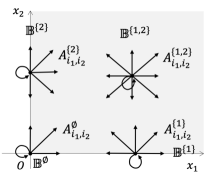
Figure 1: Transition probability blocks

Since the level process is skip free, for every $\boldsymbol{x},\boldsymbol{x}^{\prime}\in\mathbb{Z}_{+}^{2}$, $P_{\boldsymbol{x},\boldsymbol{x}^{\prime}}$ is given by

$$P_{\boldsymbol{x},\boldsymbol{x}^{\prime}}=\left\{\begin{array}[]{ll}A^{\alpha}_{\boldsymbol{x}^{\prime}-\boldsymbol{x}},&\mbox{if $\boldsymbol{x}\in\mathbb{B}^{\alpha}$ for some $\alpha\in\mathscr{I}_{2}$ and $\boldsymbol{x}^{\prime}-\boldsymbol{x}\in\{-1,0,1\}^{2}$},\cr O,&\mbox{otherwise}.\end{array}\right.$$ (2.1)

We assume the following condition throughout the paper.

Assumption 2.1.

The 2d-QBD process $\{\boldsymbol{Y}_{n}\}$ is irreducible and aperiodic.

Next, we define several Markov chains derived from the 2d-QBD process. For a nonempty set $\alpha\in\mathscr{I}_{2}$, let $\{\boldsymbol{Y}^{\alpha}_{n}\}=\{(\boldsymbol{X}^{\alpha}_{n},J^{\alpha}_{n})\}$ be a process derived from the 2d-QBD process $\{\boldsymbol{Y}_{n}\}$ by removing the boundaries that are orthogonal to the $x_{i}$-axis for each $i\in\alpha$. The process $\{\boldsymbol{Y}^{\{1\}}_{n}\}$ is a Markov chain on $\mathbb{Z}\times\mathbb{Z}_{+}\times S_{0}$ whose transition probability matrix $P^{\{1\}}=(P^{\{1\}}_{\boldsymbol{x},\boldsymbol{x}^{\prime}};\boldsymbol{x},\boldsymbol{x}^{\prime}\in\mathbb{Z}\times\mathbb{Z}_{+})$ is given as

$$P^{\{1\}}_{\boldsymbol{x},\boldsymbol{x}^{\prime}}=\left\{\begin{array}[]{ll}A^{\{1\}}_{\boldsymbol{x}^{\prime}-\boldsymbol{x}},&\mbox{if $\boldsymbol{x}\in\mathbb{Z}\times\{0\}$ and $\boldsymbol{x}^{\prime}-\boldsymbol{x}\in\{-1,0,1\}\times\{0,1\}$},\cr A^{\{1,2\}}_{\boldsymbol{x}^{\prime}-\boldsymbol{x}},&\mbox{if $\boldsymbol{x}\in\mathbb{Z}\times\mathbb{N}$ and $\boldsymbol{x}^{\prime}-\boldsymbol{x}\in\{-1,0,1\}^{2}$},\cr O,&\mbox{otherwise},\end{array}\right.$$ (2.2)

where $\mathbb{N}$ is the set of all positive integers. The process $\{\boldsymbol{Y}^{\{2\}}_{n}\}$ on $\mathbb{Z}_{+}\times\mathbb{Z}\times S_{0}$ and its transition probability matrix $P^{\{2\}}=(P^{\{2\}}_{\boldsymbol{x},\boldsymbol{x}^{\prime}};\boldsymbol{x},\boldsymbol{x}^{\prime}\in\mathbb{Z}_{+}\times\mathbb{Z})$ are analogously defined. The process $\{\boldsymbol{Y}^{\{1,2\}}_{n}\}$ is a Markov chain on $\mathbb{Z}^{2}\times S_{0}$, whose transition probability matrix $P^{\{1,2\}}=(P^{\{1,2\}}_{\boldsymbol{x},\boldsymbol{x}^{\prime}};\boldsymbol{x},\boldsymbol{x}^{\prime}\in\mathbb{Z}^{2})$ is given as

$$P^{\{1,2\}}_{\boldsymbol{x},\boldsymbol{x}^{\prime}}=\left\{\begin{array}[]{ll}A^{\{1,2\}}_{\boldsymbol{x}^{\prime}-\boldsymbol{x}},&\mbox{if $\boldsymbol{x}^{\prime}-\boldsymbol{x}\in\{-1,0,1\}^{2}$},\cr O,&\mbox{otherwise}.\end{array}\right.$$ (2.3)

Regarding $X^{\{1\}}_{1,n}$ as the additive part, we see that the process $\{\boldsymbol{Y}^{\{1\}}_{n}\}=\{(X^{\{1\}}_{1,n},(X^{\{1\}}_{2,n},J^{\{1\}}_{n}))\}$ is a Markov additive process (MA-process for short) with the background state $(X^{\{1\}}_{2,n},J^{\{1\}}_{n})$ (with respect to MA-processes, see, for example, Ney and Nummelin [10]). The process $\{\boldsymbol{Y}^{\{2\}}_{n}\}=\{(X^{\{2\}}_{2,n},(X^{\{2\}}_{1,n},J^{\{2\}}_{n}))\}$ is also an MA-process, where $X^{\{2\}}_{2,n}$ is the additive part and $(X^{\{2\}}_{1,n},J^{\{2\}}_{n})$ the background state, and $\{\boldsymbol{Y}^{\{1,2\}}_{n}\}=\{(X^{\{1,2\}}_{1,n},X^{\{1,2\}}_{2,n}),J^{\{1,2\}}_{n})\}$ an MA-process, where $(X^{\{1,2\}}_{1,n},X^{\{1,2\}}_{2,n})$ the additive part and $J^{\{1,2\}}_{n}$ the background state. We call them the induced MA-processes derived from the original 2d-QBD process. Let $\{\bar{A}^{\{1\}}_{i}:i\in\{-1,0,1\}\}$ be the Markov additive kernel (MA-kernel for short) of the induced MA-process $\{\boldsymbol{Y}^{\{1\}}_{n}\}$, which is the set of transition probability blocks and defined as, for $i\in\{-1,0,1\}$,

$$\bar{A}^{\{1\}}_{i}=\left(\bar{A}^{\{1\}}_{i,(x_{2},x_{2}^{\prime})};x_{2},x_{2}^{\prime}\in\mathbb{Z}_{+}\right),$$

$$\bar{A}^{\{1\}}_{i,(x_{2},x_{2}^{\prime})}=\left\{\begin{array}[]{ll}A^{\{1\}}_{i,x_{2}^{\prime}-x_{2}},&\mbox{if $x_{2}=0$ and $x_{2}^{\prime}-x_{2}\in\{0,1\}$},\cr A^{\{1,2\}}_{i,x_{2}^{\prime}-x_{2}},&\mbox{if $x_{2}\geq 1$ and $x_{2}^{\prime}-x_{2}\in\{-1,0,1\}$},\cr O,&\mbox{otherwise}.\end{array}\right.$$

Let $\{\bar{A}^{\{2\}}_{i}:i\in\{-1,0,1\}\}$ be the MA-kernel of $\{\boldsymbol{Y}^{\{2\}}_{n}\}$, defined in the same way. With respect to $\{\boldsymbol{Y}^{\{1,2\}}_{n}\}$, the MA-kernel is given by $\{A^{\{1,2\}}_{i_{1},i_{2}}:i_{1},i_{2}\in\{-1,0,1\}\}$. We assume the following condition throughout the paper.

Assumption 2.2.

The induced MA-processes $\{\boldsymbol{Y}^{\{1\}}_{n}\}$, $\{\boldsymbol{Y}^{\{2\}}_{n}\}$ and $\{\boldsymbol{Y}^{\{1,2\}}_{n}\}$ are irreducible and aperiodic.

According to [16], we assume several other technical conditions for the induced MA-process $\{\boldsymbol{Y}_{n}^{\{1,2\}}\}$, concerning irreducibility and aperiodicity on subspaces. Let $\{\boldsymbol{Y}^{+}_{n}\}=\{(\boldsymbol{X}^{+}_{n},J^{+}_{n})\}$ be a lossy Markov chain derived from the induced MA-process $\{\boldsymbol{Y}^{\{1,2\}}_{n}\}$ by restricting the state space of the additive part to $\mathbb{N}^{2}$. The process $\{\boldsymbol{Y}^{+}_{n}\}$ is a Markov chain on the state space $\mathbb{N}^{2}\times S_{0}$ whose transition probability matrix $P^{+}$ is given as $P^{+}=(P^{\{1,2\}}_{\boldsymbol{x},\boldsymbol{x}^{\prime}};\boldsymbol{x},\boldsymbol{x}^{\prime}\in\mathbb{N}^{2})$, where $P^{+}$ is strictly substochastic. We assume the following condition throughout the paper.

Assumption 2.3.

$\{\boldsymbol{Y}^{+}_{n}\}$ is irreducible and aperiodic.

For $k\in\mathbb{Z}$, let $\mathbb{Z}_{\leq k}$ and $\mathbb{Z}_{\geq k}$ be the set of integers less than or equal to $k$ and that of integers greater than or equal to $k$, respectively. We assume the following condition throughout the paper. For what this assumption implies, see Remark 3.1 of [16].

Assumption 2.4.

• The lossy Markov chain derived from the induced MA-process $\{\boldsymbol{Y}^{\{1,2\}}_{n}\}$ by restricting the state space to $\mathbb{Z}_{\leq 0}\times\mathbb{Z}_{\geq 0}\times S_{0}$ is irreducible and aperiodic.

• The lossy Markov chain derived from $\{\boldsymbol{Y}^{\{1,2\}}_{n}\}$ by restricting the state space to $\mathbb{Z}_{\geq 0}\times\mathbb{Z}_{\leq 0}\times S_{0}$ is irreducible and aperiodic.

The stability condition of the 2d-QBD process has already been obtained in [13]. Let $a^{\{1\}}$, $a^{\{2\}}$ and $\boldsymbol{a}^{\{1,2\}}=(a^{\{1,2\}}_{1},a^{\{1,2\}}_{2})$ be the mean drifts of the additive part in the induced MA-processes $\{\boldsymbol{Y}^{\{1\}}_{n}\}$, $\{\boldsymbol{Y}^{\{2\}}_{n}\}$ and $\{\boldsymbol{Y}^{\{1,2\}}_{n}\}$, respectively. By Corollary 3.1 of [13], the stability condition of the 2d-QBD process $\{\boldsymbol{Y}_{n}\}$ is given as follows:

Lemma 2.1.

• In the case where $a^{\{1,2\}}_{1}<0$ and $a^{\{1,2\}}_{2}<0$, the 2d-QBD process $\{\boldsymbol{Y}_{n}\}$ is positive recurrent if $a^{\{1\}}<0$ and $a^{\{2\}}<0$, and it is transient if either $a^{\{1\}}>0$ or $a^{\{2\}}>0$.

• In the case where $a^{\{1,2\}}_{1}\geq 0$ and $a^{\{1,2\}}_{2}<0$, $\{\boldsymbol{Y}_{n}\}$ is positive recurrent if $a^{\{1\}}<0$, and it is transient if $a^{\{1\}}>0$.

• In the case where $a^{\{1,2\}}_{1}<0$ and $a^{\{1,2\}}_{2}\geq 0$, $\{\boldsymbol{Y}_{n}\}$ is positive recurrent if $a^{\{2\}}<0$, and it is transient if $a^{\{2\}}>0$.

• If one of $a^{\{1,2\}}_{1}$ and $a^{\{1,2\}}_{2}$ is positive and the other is non-negative, then $\{\boldsymbol{Y}_{n}\}$ is transient.

For the explicit expression of the mean drifts, see Section 3.1 of [13] and its related parts. We assume the following condition throughout the paper.

Assumption 2.5.

The condition in Lemma 2.1 that ensures the 2d-QBD process $\{\boldsymbol{Y}_{n}\}$ is positive recurrent holds.

Denote by $\boldsymbol{\nu}$ the stationary distribution of $\{\boldsymbol{Y}_{n}\}$, where $\boldsymbol{\nu}=(\boldsymbol{\nu}_{\boldsymbol{x}},\boldsymbol{x}\in\mathbb{Z}_{+}^{2})$, $\boldsymbol{\nu}_{\boldsymbol{x}}=(\nu_{(\boldsymbol{x},j)},j\in S_{0})$ and $\nu_{(\boldsymbol{x},j)}$ is the stationary probability that the 2d-QBD process is in the state $(\boldsymbol{x},j)$.

2.2 Main results

Let $\bar{A}^{\{1\}}_{*}(z)$ and $\bar{A}^{\{2\}}_{*}(z)$ be the matrix generating functions of the MA-kernels of $\{\boldsymbol{Y}^{\{1\}}_{n}\}$ and $\{\boldsymbol{Y}^{\{2\}}_{n}\}$, respectively, defined as

$$\bar{A}^{\{1\}}_{*}(z)=\sum_{i\in\{-1,0,1\}}z^{i}\bar{A}^{\{1\}}_{i},\quad\bar{A}^{\{2\}}_{*}(z)=\sum_{i\in\{-1,0,1\}}z^{i}\bar{A}^{\{2\}}_{i}.$$

The matrix generating function of the MA-kernel of $\{\boldsymbol{Y}^{\{1,2\}}_{n}\}$ is given by $A^{\{1,2\}}_{*,*}(z_{1},z_{2})$, defined as

$$A^{\{1,2\}}_{*,*}(z_{1},z_{2})=\sum_{i_{1},i_{2}\in\{-1,0,1\}}z_{1}^{i_{1}}z_{2}^{i_{2}}A^{\{1,2\}}_{i_{1},i_{2}}.$$

Let $\Gamma^{\{1\}}$, $\Gamma^{\{2\}}$ and $\Gamma^{\{1,2\}}$ be domains in which the convergence parameters of $\bar{A}^{\{1\}}_{*}(e^{\theta_{1}})$, $\bar{A}^{\{2\}}_{*}(e^{\theta_{2}})$ and $A^{\{1,2\}}_{*,*}(e^{\theta_{1}},e^{\theta_{2}})$ are greater than $1$, respectively, i.e.,

$$\Gamma^{\{1\}}=\{(\theta_{1},\theta_{2})\in\mathbb{R}^{2}:\mbox{\rm cp}(\bar{A}^{\{1\}}_{*}(e^{\theta_{1}}))>1\},\quad\Gamma^{\{2\}}=\{(\theta_{1},\theta_{2})\in\mathbb{R}^{2}:\mbox{\rm cp}(\bar{A}^{\{2\}}_{*}(e^{\theta_{2}}))>1\},$$

$$\Gamma^{\{1,2\}}=\{(\theta_{1},\theta_{2})\in\mathbb{R}^{2}:\mbox{\rm cp}(A^{\{1,2\}}_{*,*}(e^{\theta_{1}},e^{\theta_{2}}))>1\},$$

where, for a nonnegative square matrix $A$ with a finite or countable dimension, $\mbox{\rm cp}(A)$ denote the convergence parameter of $A$, i.e., $\mbox{\rm cp}(A)=\sup\{r\in\mathbb{R}_{+}:\sum_{n=0}^{\infty}r^{n}A^{n}<\infty,\ \mbox{entry-wise}\}$. We have $\mbox{\rm cp}(A^{\{1,2\}}_{*,*}(e^{\theta_{1}},e^{\theta_{2}}))=\mbox{\rm spr}(A^{\{1,2\}}_{*,*}(e^{\theta_{1}},e^{\theta_{2}}))^{-1}$, where for a square complex matrix $A$, $\mbox{\rm spr}(A)$ is the spectral radius of $A$. By Lemma A.1 of Ozawa [15], $\mbox{\rm cp}(\bar{A}^{\{1\}}_{*}(e^{\theta}))^{-1}$ and $\mbox{\rm cp}(\bar{A}^{\{2\}}_{*}(e^{\theta}))^{-1}$ are log-convex in $\theta$, and the closures of $\Gamma^{\{1\}}$ and $\Gamma^{\{2\}}$ are convex sets; $\mbox{\rm spr}(A^{\{1,2\}}_{*}(e^{\theta_{1}},e^{\theta_{2}}))$ is also log-convex in $(\theta_{1},\theta_{2})$, and the closure of $\Gamma^{\{1,2\}}$ is a convex set. Furthermore, by Proposition B.1 of Ozawa [15], $\Gamma^{\{1,2\}}$ is bounded under Assumption 2.2. We depict an example of the domains $\Gamma^{\{1,2\}}$, $\Gamma^{\{1\}}$ and $\Gamma^{\{2\}}$ in Fig. 2.

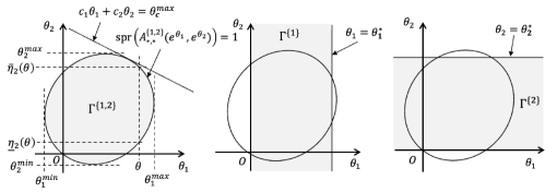
Figure 2: Domains $\Gamma^{\{1,2\}}$, $\Gamma^{\{1\}}$ and $\Gamma^{\{2\}}$

We define several extreme values and functions with respect to the domains. For $i\in\{1,2\}$, define $\theta_{i}^{min}$ and $\theta_{i}^{max}$ as

$$\theta_{i}^{min}=\inf\{\theta_{i}\in\mathbb{R}:(\theta_{1},\theta_{2})\in\Gamma^{\{1,2\}}\},\quad\theta_{i}^{max}=\sup\{\theta_{i}\in\mathbb{R}:(\theta_{1},\theta_{2})\in\Gamma^{\{1,2\}}\},$$

and for a direction vector $\boldsymbol{c}=(c_{1},c_{2})\in\mathbb{N}^{2}$, $\theta_{\boldsymbol{c}}^{max}$ as

$$\theta_{\boldsymbol{c}}^{max}=\sup\{c_{1}\theta_{1}+c_{2}\theta_{2}:(\theta_{1},\theta_{2})\in\Gamma^{\{1,2\}}\}.$$

By Lemma 2.3 of [12], under Assumption 2.5, the domain $\Gamma^{\{1,2\}}$ includes positive points, i.e., $\{(\theta_{1},\theta_{2})\in\Gamma^{\{1,2\}}:\theta_{1}>0,\,\theta_{2}>0\}\neq\emptyset$, and this implies $\theta_{\boldsymbol{c}}^{max}>0$ for every direction vector $\boldsymbol{c}\in\mathbb{N}^{2}$. For $\theta_{1}\in[\theta_{1}^{min},\theta_{1}^{max}]$, there exist two real solutions to equation $\mbox{\rm spr}(A^{\{1,2\}}_{*,*}(e^{\theta_{1}},e^{\theta_{2}}))=1$, counting multiplicity. Denote them by $\theta_{2}=\underline{\eta}_{2}(\theta_{1})$ and $\theta_{2}=\bar{\eta}_{2}(\theta_{1})$, respectively, where $\underline{\eta}_{2}(\theta_{1})\leq\bar{\eta}_{2}(\theta_{1})$. For $\theta_{2}\in[\theta_{2}^{min},\theta_{2}^{max}]$, also denote by $\theta_{1}=\underline{\eta}_{1}(\theta_{2})$ and $\theta_{1}=\bar{\eta}_{1}(\theta_{2})$ the two real solutions to the equation $\mbox{\rm spr}(A^{\{1,2\}}_{*,*}(e^{\theta_{1}},e^{\theta_{2}}))=1$, where $\underline{\eta}_{1}(\theta_{2})\leq\bar{\eta}_{1}(\theta_{2})$. For $i\in\{1,2\}$, define $\theta_{i}^{*}$ as

$$\theta_{i}^{*}=\sup\{\theta_{i}\in\mathbb{R}:(\theta_{1},\theta_{2})\in\Gamma^{\{i\}}\}.$$

For another characterization of $\theta_{i}^{*}$, see Proposition 3.7 of Ozawa [11], where $\theta_{i}^{*}$ is denoted by $z_{0}$. By Lemma 2.5 of [12] and its related parts, under Assumption 2.5, we have $\theta_{i}^{*}>0$ for $i\in\{1,2\}$.

In terms of these points and functions, we geometrically classify the model into four types according to Section 4.1 of [16]. Define two points $\mathrm{Q}_{1}$ and $\mathrm{Q}_{2}$ as $\mathrm{Q}_{1}=(\theta_{1}^{*},\bar{\eta}_{2}(\theta_{1}^{*}))$ and $\mathrm{Q}_{2}=(\bar{\eta}_{1}(\theta_{2}^{*}),\theta_{2}^{*})$, respectively. Using these points, we define the following classification (see Fig. 3).

• Type 1: $\theta_{1}^{*}\geq\bar{\eta}_{1}(\theta_{2}^{*})$ and $\bar{\eta}_{2}(\theta_{1}^{*})\leq\theta_{2}^{*}$,
  Type 2: $\theta_{1}^{*}<\bar{\eta}_{1}(\theta_{2}^{*})$ and $\bar{\eta}_{2}(\theta_{1}^{*})>\theta_{2}^{*}$,
  Type 3: $\theta_{1}^{*}\geq\bar{\eta}_{1}(\theta_{2}^{*})$ and $\bar{\eta}_{2}(\theta_{1}^{*})>\theta_{2}^{*}$,
  Type 4: $\theta_{1}^{*}<\bar{\eta}_{1}(\theta_{2}^{*})$ and $\bar{\eta}_{2}(\theta_{1}^{*})\leq\theta_{2}^{*}$.

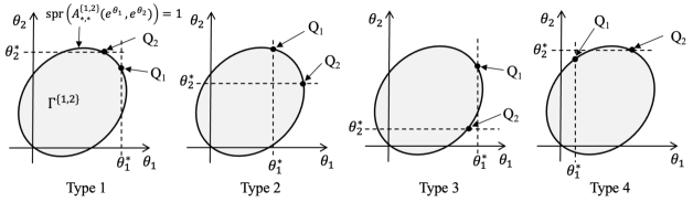
Figure 3: Classification

By Proposition 2.3 of [16], for any direction vector $\boldsymbol{c}=(c_{1},c_{2})\in\mathbb{N}^{2}$, the asymptotic decay rate in the direction $\boldsymbol{c}$ is space homogeneous. Hence, we denote it by $\xi_{\boldsymbol{c}}$, which satisfies, for any $(\boldsymbol{x},j)\in\mathbb{Z}_{+}^{2}\times S_{0}$,

$$\xi_{\boldsymbol{c}}=-\lim_{k\to\infty}\frac{1}{k}\log\nu_{(k\boldsymbol{c}+\boldsymbol{x},j)}.$$ (2.4)

The asymptotic decay rate $\xi_{\boldsymbol{c}}$ has already been obtained in [16], and as described in Section 4.1 of [16], it is given as follows.

Theorem 2.1.

Let $\boldsymbol{c}=(c_{1},c_{2})$ be an arbitrary direction vector in $\mathbb{N}^{2}$.

• Type 1:

  $$\xi_{\boldsymbol{c}}=\left\{\begin{array}[]{ll}c_{1}\theta_{1}^{*}+c_{2}\bar{\eta}_{2}(\theta_{1}^{*})&\mbox{if $-\frac{c_{1}}{c_{2}}<\bar{\eta}^{\prime}_{2}(\theta_{1}^{*})$},\cr\theta_{\boldsymbol{c}}^{max}&\mbox{if $\bar{\eta}^{\prime}_{2}(\theta_{1}^{*})\leq-\frac{c_{1}}{c_{2}}\leq\bar{\eta}^{\prime}_{1}(\theta_{2}^{*})^{-1}$},\cr c_{1}\bar{\eta}_{1}(\theta_{2}^{*})+c_{2}\theta_{2}^{*}&\mbox{if $-\frac{c_{1}}{c_{2}}>\bar{\eta}^{\prime}_{1}(\theta_{2}^{*})^{-1}$},\end{array}\right.$$

  where $\bar{\eta}^{\prime}_{2}(x)=\frac{d}{dx}\bar{\eta}_{2}(x)$ and $\bar{\eta}^{\prime}_{1}(x)=\frac{d}{dx}\bar{\eta}_{1}(x)$.

• Type 2:

  $$\xi_{\boldsymbol{c}}=\left\{\begin{array}[]{ll}c_{1}\theta_{1}^{*}+c_{2}\bar{\eta}_{2}(\theta_{1}^{*})&\mbox{if $-\frac{c_{1}}{c_{2}}\leq\frac{\theta_{2}^{*}-\bar{\eta}_{2}(\theta_{1}^{*})}{\bar{\eta}_{1}(\theta_{2}^{*})-\theta_{1}^{*}}$},\cr c_{1}\bar{\eta}_{1}(\theta_{2}^{*})+c_{2}\theta_{2}^{*}&\mbox{if $-\frac{c_{1}}{c_{2}}>\frac{\theta_{2}^{*}-\bar{\eta}_{2}(\theta_{1}^{*})}{\bar{\eta}_{1}(\theta_{2}^{*})-\theta_{1}^{*}}$}.\end{array}\right.$$

• Type 3: $\xi_{\boldsymbol{c}}=c_{1}\bar{\eta}_{1}(\theta_{2}^{*})+c_{2}\theta_{2}^{*}$.

• Type 4: $\xi_{\boldsymbol{c}}=c_{1}\theta_{1}^{*}+c_{2}\bar{\eta}_{2}(\theta_{1}^{*})$.

Under Assumption 2.5, since $\Gamma^{\{1,2\}}\cap\Gamma^{\{1\}}\cap\Gamma^{\{2\}}$ includes positive points, we have $\xi_{\boldsymbol{c}}>0$ for every $\boldsymbol{c}\in\mathbb{N}^{2}$. The asymptotic decay function $h_{\boldsymbol{c}}(k)$ in the direction $\boldsymbol{c}$ is defined as the function that satisfies, for some positive vector $\boldsymbol{g}_{\boldsymbol{c}}$,

$$\lim_{k\to\infty}\frac{\boldsymbol{\nu}_{k\boldsymbol{c}}}{h_{\boldsymbol{c}}(k)}=\boldsymbol{g}_{\boldsymbol{c}}.$$ (2.5)

It is given as follows.

Theorem 2.2.

Let $\boldsymbol{c}$ be an arbitrary direction vector in $\mathbb{N}^{2}$. Then, the asymptotic decay function $h_{\boldsymbol{c}}(k)$ is given as

$$h_{\boldsymbol{c}}(k)=\left\{\begin{array}[]{ll}k^{-\frac{1}{2}}e^{-\xi_{\boldsymbol{c}}k}&\mbox{if $\bar{\eta}^{\prime}_{2}(\theta_{1}^{*})<-\frac{c_{1}}{c_{2}}<\bar{\eta}^{\prime}_{1}(\theta_{2}^{*})^{-1}$ in Type 1},\cr e^{-\xi_{\boldsymbol{c}}k}&\mbox{otherwise}.\end{array}\right.$$ (2.6)

Except for the case where $\bar{\eta}^{\prime}_{2}(\theta_{1}^{*})\leq-\frac{c_{1}}{c_{2}}\leq\bar{\eta}^{\prime}_{1}(\theta_{2}^{*})^{-1}$ in Type 1, Theorem 2.2 has already been proved in [16], see Theorem 3.2 therein. Hence, to this end, it suffices to prove the following proposition.

Proposition 2.1.

Assume Type 1 and set $\boldsymbol{c}=(c_{1},c_{2})=(1,1)$. Then, the asymptotic decay function $h_{\boldsymbol{c}}(k)$ is given as

$$h_{\boldsymbol{c}}(k)=\left\{\begin{array}[]{ll}k^{-\frac{1}{2}}e^{-\theta_{\boldsymbol{c}}^{max}k}&\mbox{if $\bar{\eta}^{\prime}_{2}(\theta_{1}^{*})<-\frac{c_{1}}{c_{2}}=-1<\bar{\eta}^{\prime}_{1}(\theta_{2}^{*})^{-1}$},\cr e^{-\theta_{\boldsymbol{c}}^{max}k}&\mbox{if $\bar{\eta}^{\prime}_{2}(\theta_{1}^{*})=-1$ or $\bar{\eta}^{\prime}_{1}(\theta_{2}^{*})=-1$}.\end{array}\right.$$ (2.7)

From this proposition, we can obtain the same result for a general direction vector $\boldsymbol{c}\in\mathbb{N}^{2}$, by using the block state process derived from the original 2d-QBD process; See Section 3.3 of [16]. We, therefore, prove the proposition in Section 4. The asymptotic decay function is space-homogeneous with respect to the level of the 2d-QBD process, as follows. We prove this corollary in Section 4.4.

Corollary 2.1.

Let $\boldsymbol{c}$ be an arbitrary direction vector in $\mathbb{N}^{2}$. For every $\boldsymbol{x}\in\mathbb{Z}_{+}^{2}$, the asymptotic function $h_{\boldsymbol{c}}(k)$ in Theorem 2.2 satisfies, for some positive vector $\boldsymbol{g}_{\boldsymbol{c},\boldsymbol{x}}$,

$$\lim_{k\to\infty}\frac{\boldsymbol{\nu}_{k\boldsymbol{c}+\boldsymbol{x}}}{h_{\boldsymbol{c}}(k)}=\boldsymbol{g}_{\boldsymbol{c},\boldsymbol{x}}.$$ (2.8)

Remark 2.1.

When the model is a 2d-RRW without a background process, the result of Theorem 2.2 coincides with that of Theorem 1 of Malyshev [7] (also see Theorem 7.1 of [2] ). For the correspondence between them, see Section 4.1 of [16].

3 Preliminaries

Let $z$ and $w$ be complex valuables unless otherwise stated. For a positive number $r$, denote by $\Delta_{r}$ the open disk of center $0$ and radius $r$ on the complex plain, and $\partial\Delta_{r}$ the circle of the same center and radius. For $a,b\in\mathbb{R}_{+}$ such that $a<b$, let $\Delta_{a,b}$ be an open annular domain on $\mathbb{C}$ defined as $\Delta_{a,b}=\{z\in\mathbb{C}:a<|z|<b\}$. We denote by $\bar{\Delta}_{a,b}$ the closure of $\Delta_{a,b}$. For $r>0$, $\varepsilon>0$ and $\theta\in[0,\pi/2)$, define

$$\tilde{\Delta}_{r}(\varepsilon,\theta)=\{z\in\mathbb{C}:|z|<r+\varepsilon,\ z\neq r,\ |\arg(z-r)|>\theta\}.$$

For $r>0$, we denote by “$\tilde{\Delta}_{r}\ni z\to r$” that $\tilde{\Delta}_{r}(\varepsilon,\theta)\ni z\to r$ for some $\varepsilon>0$ and some $\theta\in[0,\pi/2)$. In the rest of the paper, instead of proving that a function $f(z)$ is analytic in $\tilde{\Delta}_{r}(\varepsilon,\theta)$ for some $\varepsilon>0$ and $\theta\in[0,\pi/2)$, we often demonstrate that the function $f(z)$ is analytic in ${\Delta}_{r}$ and on $\partial\Delta_{r}\setminus\{r\}$.

In order to give general results, this section is described independently from other parts of the paper.

3.1 Analytic extension of a G-matrix function

First, we define a G-matrix function according to [12]. For $i,j\in\{-1,0,1\}$, let $A_{i,j}$ be a substochastic matrix with a finite dimension $s_{0}$, and define the following matrix functions:

$$A_{*,j}(z)=\sum_{i\in\{-1,0,1\}}z^{i}A_{i,j},\ j=-1,0,1,\quad A_{*,*}(z,w)=\sum_{i,j\in\{-1,0,1\}}z^{i}w^{j}A_{i,j}.$$

We assume the following condition.

Assumption 3.1.

$A_{*,*}(1,1)$ is stochastic.

Let $\chi(z,w)$ be the spectral radius of $A_{*.*}(z,w)$, i.e., $\chi(z,w)=\mbox{\rm spr}(A_{*,*}(z,w))$, and $\Gamma$ be a domain on $\mathbb{R}^{2}$ defined as

$$\Gamma=\{(\theta_{1},\theta_{2})\in\mathbb{R}^{2}:\chi(e^{\theta_{1}},e^{\theta_{2}})<1\}.$$

We assume the following condition.

Assumption 3.2.

The Markov modulated random walk on $\mathbb{Z}^{2}\times\{1,2,...,s_{0}\}$ governed by $\{A_{i,j}:i,j\in\{-1,0,1\}\}$ is irreducible and aperiodic.

Under this assumption, $A_{*,*}(1,1)$ is also irreducible and aperiodic. Furthermore, by Lemma 2.2 of [12], $\Gamma$ is bounded. Since $\chi(e^{\theta_{1}},e^{\theta_{2}})$ is convex in $(\theta_{1},\theta_{2})\in\mathbb{R}^{2}$, the closure of $\Gamma$ is a convex set. Define extreme points $\theta_{1}^{min}$ and $\theta_{1}^{max}$ as follows:

$$\theta_{1}^{min}=\inf_{(\theta_{1},\theta_{2})\in\Gamma}\theta_{1},\quad\theta_{1}^{max}=\sup_{(\theta_{1},\theta_{2})\in\Gamma}\theta_{1}.$$

For $\theta_{1}\in[\theta_{1}^{min},\theta_{1}^{max}]$, let $\underline{\theta}_{2}(\theta_{1})$ and $\bar{\theta}_{2}(\theta_{1})$ be the two real solutions to equation $\chi(e^{\theta_{1}},e^{\theta_{2}})=1$, counting multiplicity, where $\underline{\theta}_{2}(\theta_{1})\leq\bar{\theta}_{2}(\theta_{1})$. For $n\geq 1$, define the following set of index sequences:

$$\mathscr{I}_{n}=\biggl{\{}\boldsymbol{i}_{(n)}\in\{-1,0,1\}^{n}:\ \sum_{l=1}^{k}i_{l}\geq 0\ \mbox{for $k\in\{1,2,...,n-1\}$}\ \mbox{and}\sum_{l=1}^{n}i_{l}=-1\biggr{\}},$$

where $\boldsymbol{i}_{(n)}=(i_{1},i_{2},...,i_{n})$, and define the following matrix function:

$$D_{n}(z)=\sum_{\boldsymbol{i}_{(n)}\in\mathscr{I}_{n}}A_{*,i_{1}}(z)A_{*,i_{2}}(z)\cdots A_{*,i_{n}}(z).$$

Define a matrix function $G(z)$ as

$$G(z)=\sum_{n=1}^{\infty}D_{n}(z).$$

By Lemma 4.1 of [12], this matrix series absolutely converges entry-wise in $z\in\bar{\Delta}_{e^{\theta_{1}^{min}},e^{\theta_{1}^{max}}}$. We call this $G(z)$ the G-matrix function generated from $\{A_{i,j}:i,j\in\{-1,0,1\}\}$. For $z\in\bar{\Delta}_{e^{\theta_{1}^{min}},e^{\theta_{1}^{max}}}$, $G(z)$ satisfies the inequality $|G(z)|\leq G(|z|)$ and the following matrix quadratic equation:

$$A_{*,-1}(z)+A_{*,0}(z)G(z)+A_{*,1}(z)G(z)^{2}=G(z).$$ (3.1)

Furthermore, for $x\in[e^{\theta_{1}^{min}},e^{\theta_{1}^{max}}]$, $G(x)$ is the minimum nonnegative solution to equation (3.1). Hence, $G(z)$ is an extension of a usual G-matrix in the queueing theory, see, for example, [8]. By Proposition 2.5 of [12], we see that, for $x\in[e^{\theta_{1}^{min}},e^{\theta_{1}^{max}}]$, the Perron-Frobenius eigenvalue of $G(x)$ is given by $e^{\underline{\theta}_{2}(\log x)}$, i.e., $\mbox{\rm spr}(G(x))=e^{\underline{\theta}_{2}(\log x)}$. By Lemma 4.1 of [12], $G(z)$ satisfies

$$I-A_{*,*}(z,w) =w^{-1}\left(I-A_{*,0}(z)-wA_{*,1}(z)+A_{*,1}(z)G(z)\right)(wI-G(z)).$$ (3.2)

By Lemma 4.2 of [12], the following property holds true for $G(z)$.

Lemma 3.1.

$G(z)$ is entry-wise analytic in the open annular domain $\Delta_{e^{\theta_{1}^{min}},e^{\theta_{1}^{max}}}$.

We give the eigenvalues of $G(z)$ according to [12]. Note that our final aim in this subsection is to give an analytic extension of $G(z)$ through its Jordan canonical form without assuming all the eigenvalues of $G(z)$ are distinct. In [12], the eigenvalues were assumed to be distinct. Define a matrix function $L(z,w)$ as

$$L(z,w)=zw(I-A_{*,*}(z,w)).$$

Each entry of $L(z,w)$ is a polynomial in $z$ and $w$ with at most degree $2$ for each variable. We use a notation $\Xi$, defined as follows. Let $f(z,w)$ be an irreducible polynomial in $z$ and $w$ and assume its degree with respect to $w$ is $m\geq 1$. Let $a(z)$ be the coefficient of $w^{m}$ in $f(z,w)$. Define a point set $\Xi(f)$ as

$$\Xi(f) =\{z\in\mathbb{C}:\mbox{$a(z)=0$ or ($f(z,w)=0$ and $f_{w}(z,w)=0$ for some $w\in\mathbb{C}$)}\},$$

where $f_{w}(z,w)=(\partial/\partial w)f(z,w)$. Each point in $\Xi(f)$ is an algebraic singularity of the algebraic function $w=\alpha(z)$ defined by polynomial equation $f(z,w)=0$. For each point $z\in\mathbb{C}\setminus\Xi(f)$, $f(z,w)=0$ has just $m$ distinct solutions, which correspond to the $m$ branches of the algebraic function. Let $\phi(z,w)$ be a polynomial in $z$ and $w$ defined as

$$\phi(z,w)=\det L(z,w)$$

and $m_{\phi}$ its degree with respect to $w$, where $s_{0}\leq m_{\phi}\leq 2s_{0}$. Let $\alpha_{1}(z)$, $\alpha_{2}(z)$, …, $\alpha_{m_{\phi}}(z)$ be the $m_{\phi}$ branches of the algebraic function $w=\alpha(z)$ defined by the polynomial equation $\phi(z,w)=0$, counting multiplicity. We number the brunches so that they satisfy the following:

• For every $z\in\bar{\Delta}_{e^{\theta_{1}^{min}},e^{\theta_{1}^{max}}}$ and for every $k\in\{1,2,...,s_{0}\}$, $|\alpha_{k}(z)|\leq e^{\underline{\theta}_{2}(\log|z|)}$.

• For every $z\in\bar{\Delta}_{e^{\theta_{1}^{min}},e^{\theta_{1}^{max}}}$ and for every $k\in\{s_{0}+1,s_{0}+2,...,m_{\phi}\}$, $|\alpha_{k}(z)|\geq e^{\bar{\theta}_{2}(\log|z|)}$.

• For every $x\in[e^{\theta_{1}^{min}},e^{\theta_{1}^{max}}]$, $\alpha_{s_{0}}(x)=e^{\underline{\theta}_{2}(\log x)}$ and $\alpha_{s_{0}+1}(x)=e^{\bar{\theta}_{2}(\log x)}$.

This is possible by Lemma 4.3 of [12]. By Lemmas 4.3 and 4.4 of [12], the G-matrix function $G(z)$ satisfies the following property.

Lemma 3.2.

For every $z\in\bar{\Delta}_{e^{\theta_{1}^{min}},e^{\theta_{1}^{max}}}$, the eigenvalues of $G(z)$ are given by $\alpha_{1}(z)$, $\alpha_{2}(z)$, …, $\alpha_{s_{0}}(z)$.

Without loss of generality, we assume that, for some $n_{\phi}\in\mathbb{N}$ and $l_{1},l_{2},...,l_{n_{\phi}}\in\mathbb{N}$, the polynomial $\phi(z,w)$ is factorized as

$$\phi(z,w)=f_{1}(z,w)^{l_{1}}f_{2}(z,w)^{l_{2}}\cdots f_{n_{\phi}}(z,w)^{l_{n_{\phi}}},$$ (3.3)

where $f_{k}(z,w),\,k=1,2,...,n_{\phi}$, are irreducible polynomials in $z$ and $w$ and they are relatively prime. Since the field of coefficients of polynomials is $\mathbb{C}$, this factorization is unique. For every $k\in\{1,2,...,m_{\phi}\}$, $\alpha_{k}(z)$ is a branch of the algebraic function $w=\alpha(z)$ defined by the polynomial equation $f_{n}(z,w)=0$ for some $n\in\{1,2,...,n_{\phi}\}$. We denote such $n$ by $q(k)$, i.e., $f_{q(k)}(z,\alpha_{k}(z))=0$. Since $\alpha_{s_{0}}(z)$ is the Perron-Frobenius eigenvalue of $G(z)$ when $z\in[e^{\theta_{1}^{min}},e^{\theta_{1}^{max}}]$, the multiplicity of $\alpha_{s_{0}}(z)$ is one and we have $l_{q(s_{0})}=1$. Define a point set $\mathcal{E}_{1}$ as

$$\mathcal{E}_{1}=\bigcup_{n=1}^{n_{\phi}}\Xi(f_{n}).$$

Since, for every $n$, the polynomial $f_{n}(z,w)$ is irreducible and not identically zero, the point set $\mathcal{E}_{1}$ is finite. Every branch $\alpha_{k}(z)$ is analytic in $\mathbb{C}\setminus\mathcal{E}_{1}$. Define a point set $\mathcal{E}_{2}$ as

$$\mathcal{E}_{2} =\{z\in\mathbb{C}\setminus\mathcal{E}_{1}:\mbox{$f_{n}(z,w)=f_{n^{\prime}}(z,w)=0$ }$$

$$\qquad\qquad\mbox{for some $n,n^{\prime}\in\{1,2,...,n_{\phi}\}$ such that $n\neq n^{\prime}$ and for some $w\in\mathbb{C}$}\}.$$

Since, for any $n,n^{\prime}$ such that $n\neq n^{\prime}$, $f_{n}(z,w)$ and $f_{n^{\prime}}(z,w)$ are relatively prime, the point set $\mathcal{E}_{2}$ is finite. Note that every branch $\alpha_{k}(z)$ is analytic in a neighborhood of any $z_{0}\in\mathcal{E}_{2}$. For every $k\in\{1,2,...,m_{\phi}\}$ and for every $z\in\mathbb{C}\setminus(\mathcal{E}_{1}\cup\mathcal{E}_{2})$, the multiplicity of $\alpha_{k}(z)$ as a zero of $\det L(z,w)$ is equal to $l_{q(k)}$. This means that, for every $z\in\bar{\Delta}_{e^{\theta_{1}^{min}},e^{\theta_{1}^{max}}}\setminus(\mathcal{E}_{1}\cup\mathcal{E}_{2})$, the multiplicity of the eigenvalue $\alpha_{k}(z)$ of $G(z)$ is $l_{q(k)}$, which does not depend on $z$. Define a positive integer $m_{0}$ as

$$m_{0}=\sum_{k=1}^{s_{0}}\frac{1}{l_{q(k)}}.$$

This $m_{0}$ is the number of different branches in $\{\alpha_{i}(z):i=1,2,...,s_{0}\}$ when $z\in\mathbb{C}\setminus(\mathcal{E}_{1}\cup\mathcal{E}_{2})$. Denote the different branches by $\check{\alpha}_{k}(z),\,k=1,2,...,m_{0},$ so that $\check{\alpha}_{m_{0}}(z)=\alpha_{s_{0}}(z)$. Instead of using $q(k)$, we define a function $\check{q}(k)$ so that $l_{\check{q}(k)}$ indicates the multiplicity of $\check{\alpha}_{k}(z)$ when $z\in\mathbb{C}\setminus(\mathcal{E}_{1}\cup\mathcal{E}_{2})$. We always have $l_{\check{q}(m_{0})}=1$.

We give the Jordan normal form of $G(z)$. Define a domain $\Omega$ as $\Omega=\Delta_{e^{\theta_{1}^{min}},e^{\theta_{1}^{max}}}\setminus(\mathcal{E}_{1}\cup\mathcal{E}_{2})$. For $k\in\{1,2,...,m_{0}\}$ and for $i\in\{1,2,...,l_{\check{q}(k)}\}$, define a positive integer $t_{k,i}$ as

$$t_{k,i}=\min_{z\in\Omega}\dim\mbox{\rm Ker}\,(\check{\alpha}_{k}(z)I-G(z))^{i}$$

and a point set $\mathcal{G}_{k,i}$ as

$$\mathcal{G}_{k,i}=\{z\in\Omega:\dim\mbox{\rm Ker}\,(\check{\alpha}_{k}(z)I-G(z))^{i}>t_{k,i}\}.$$

Since $\check{\alpha}_{k}(z)$ and $G(z)$ are analytic in $\Omega$, we see from the proof of Theorem S6.1 of [4] that each $\mathcal{G}_{k,i}$ is an empty set or a set of discrete complex numbers. For $k\in\{1,2,...,m_{0}\}$ and $i\in\{1,2,...,l_{\check{q}(k)}\}$, define a nonnegative integer $s_{k,i}$ as

$$s_{k,i}=2t_{k,i}-t_{k,i+1}-t_{k,i-1},$$

where $t_{k,0}=0$ and $t_{k,l_{\check{q}(k)}+1}=l_{\check{q}(k)}$. For $k\in\{1,2,...,m_{0}\}$, define a positive integer $m_{k,0}$ and point set $\mathcal{E}^{G}_{k}$ as

$$m_{k,0}=t_{k,1},\qquad\mathcal{E}^{G}_{k}=\bigcup_{i=1}^{l_{\check{q}(k)}}\mathcal{G}_{k,i}.$$

When $z\in\Omega\setminus\mathcal{E}^{G}_{k}$, this $m_{k,0}$ is the number of Jordan blocks of $G(z)$ with respect to the eigenvalue $\check{\alpha}_{k}(z)$ and, for $i\in\{1,2,...,l_{\check{q}(k)}\}$, $s_{k,i}$ is the number of Jordan blocks whose dimension is $i$. Hence, the Jordan normal form of $G(z)$ takes a common form in $z\in\Omega\setminus\bigcup_{k=1}^{m_{0}}\mathcal{E}^{G}_{k}$. For $k\in\{1,2,...,m_{0}\}$ and for $i\in\{1,2,...,m_{k,0}\}$, denote by $m_{k,i}$ the dimension of the $i$-th Jordan block of $G(z)$ with respect to the eigenvalue $\check{\alpha}_{k}(z)$, where we number the Jordan blocks so that if $i\leq i^{\prime}$, $m_{k,i}\geq m_{k,i^{\prime}}$. For each $k\in\{1,2,...,m_{0}\}$, they satisfy $\sum_{i=1}^{m_{k,0}}m_{k,i}=l_{\check{q}(k)}$. Denote by $J_{n}(\lambda)$ the $n$-dimensional Jordan block of eigenvalue $\lambda$. For $z\in\Omega\setminus\bigcup_{k=1}^{m_{0}}\mathcal{E}^{G}_{k}$, the Jordan normal form of $G(z)$, $J^{G}(z)$, is given by

$$J^{G}(z)=\mbox{\rm diag}(J_{m_{k,i}}(\check{\alpha}_{k}(z)),\,k=1,2,...,m_{0},\,i=1,2,...,m_{k,0}),$$ (3.4)

where $m_{m_{0},0}=1$ and $J_{m_{m_{0},1}}(\check{\alpha}_{m_{0}}(z))=\alpha_{s_{0}}(z)$. Note that the matrix function $J^{G}(z)$ is well defined on $\mathbb{C}$ and analytic in $\mathbb{C}\setminus\mathcal{E}_{1}$. An analytic extension of $G(z)$ is given by the following theorem.

Theorem 3.1.

There exist vector functions:

$$\check{\boldsymbol{v}}_{k,i,j}^{L}(z),\,k=1,2,...,m_{0},\,i=1,2,...,m_{k,0},\,j=1,2,...,m_{k,i},$$

such that they are analytic in $\mathbb{C}\setminus\mathcal{E}_{1}$ and satisfy, for every $z\in\Delta_{e^{\theta_{1}^{min}},e^{\theta_{1}^{max}}}\setminus(\mathcal{E}_{1}\cup\mathcal{E}_{0})$,

$$G(z)=T^{L}(z)J^{G}(z)(T^{L}(z))^{-1},$$ (3.5)

where $\mathcal{E}_{0}$ is a set of discrete complex numbers and matrix function $T^{L}(z)$ is defined as

$$T^{L}(z)=\begin{pmatrix}\check{\boldsymbol{v}}_{k,i,j}^{L}(z),\,k=1,2,...,m_{0},\,i=1,2,...,m_{k,0},\,j=1,2,...,m_{k,i}\end{pmatrix}.$$

Since the proof of Theorem 3.1 is elementary and very lengthy, we give it in Appendix A. In Theorem 3.1, $\{\check{\boldsymbol{v}}_{k,i,j}^{L}(z)\}$ is the set of the generalized eigenvectors of $G(z)$, but we denote them with superscript $L$ since they are generated from the matrix function $L(z,w)$; see Appendix A. Define a point set $\mathcal{E}_{T}^{L}$ as

$$\mathcal{E}_{T}^{L}=\{z\in\mathbb{C}\setminus\mathcal{E}_{1}:\det\,T^{L}(z)=0\},$$

which is an empty set or a set of discrete complex numbers since $\det\,T^{L}(z)$ is not identically zero. Define a matrix function $\check{G}(z)$ as

$$\check{G}(z)=T^{L}(z)J^{G}(z)(T^{L}(z))^{-1}=\frac{T^{L}(z)J^{G}(z)\,\mbox{\rm adj}(T^{L}(z))}{\det(T^{L}(z))}.$$ (3.6)

Then, it is entry-wise analytic in $\mathbb{C}\setminus(\mathcal{E}_{1}\cup\mathcal{E}_{T}^{L})$. By Theorem 3.1 and the identity theorem for analytic functions, this $\check{G}(z)$ is an analytic extension of the matrix function $G(z)$. Hence, we denote $\check{G}(z)$ by $G(z)$. By Lemma 3.1, $G(z)$ is entry-wise analytic in $\Delta_{e^{\theta_{1}^{min}},e^{\theta_{1}^{max}}}$. The following corollary asserts that $G(z)$ is also analytic on the outside boundary of $\Delta_{e^{\theta_{1}^{min}},e^{\theta_{1}^{max}}}$ except for the point $z=e^{\theta_{1}^{max}}$.

Corollary 3.1.

The extended G-matrix function $G(z)$ is entry-wise analytic on $\partial\Delta_{e^{\theta_{1}^{max}}}\setminus\{e^{\theta_{1}^{max}}\}$.

Since this corollary can be proved in a manner similar to that used in the proof of Lemma 4.7 of [12], we omit it.

Denote by $\check{\boldsymbol{u}}^{L}_{m_{0},1,1}(z)$ the last row of the matrix function $(T^{L}(z))^{-1}$, and define a diagonal matrix function $J_{s_{0}}(z)$ as $J_{s_{0}}(z)=\mbox{\rm diag}\!\begin{pmatrix}0&\cdots&0&\alpha_{s_{0}}(z)\end{pmatrix}$, where $\alpha_{s_{0}}(z)=\check{\alpha}_{m_{0}}(z)$. Then, since $m_{m_{0},0}=1$ and $m_{m_{0},1}=1$, we obtain the following decomposition of $G(z)$ from (3.6):

$$G(z)=G^{\dagger}(z)+\alpha_{s_{0}}(z)\check{\boldsymbol{v}}^{L}_{m_{0},1,1}(z)\check{\boldsymbol{u}}^{L}_{m_{0},1,1}(z),$$ (3.7)

where

$$G^{\dagger}(z)=T^{L}(z)(J^{G}(z)-J_{s_{0}}(z))(T^{L}(z))^{-1}.$$

By the definition, $G(z)$ satisfies, for $n\geq 1$,

$$G(z)^{n}=G^{\dagger}(z)^{n}+\alpha_{s_{0}}(z)^{n}\check{\boldsymbol{v}}^{L}_{m_{0},1,1}(z)\check{\boldsymbol{u}}^{L}_{m_{0},1,1}(z),$$ (3.8)

and $G^{\dagger}(z)$ satisfies, for $z\in\bar{\Delta}_{e^{\theta_{1}^{min}},e^{\theta_{1}^{max}}}$, $\mbox{\rm spr}(G^{\dagger}(z))\leq\mbox{\rm spr}(G^{\dagger}(|z|))<\mbox{\rm spr}(G(|z|))=\alpha_{s_{0}}(|z|)$. Furthermore, in a neighborhood of $z=e^{\theta_{1}^{max}}$, we have $\mbox{\rm spr}(G^{\dagger}(z))<\alpha_{s_{0}}(e^{\theta_{1}^{max}})$. Since the point $z=e^{\theta_{1}^{max}}$ is a branch point of $\check{\alpha}_{m_{0}}(z)$ ($=\alpha_{s_{0}}(z)$), there exists a function $\tilde{\alpha}_{s_{0}}(\zeta)$ being analytic in a neighborhood of $\zeta=0$ and satisfying

$$\check{\alpha}_{m_{0}}(z)=\alpha_{s_{0}}(z)=\tilde{\alpha}_{s_{0}}((e^{\theta_{1}^{max}}-z)^{\frac{1}{2}}).$$

Let $\tilde{\boldsymbol{v}}_{s_{0}}(\zeta)$ be a vector function satisfying

$$L(e^{\theta_{1}^{max}}-\zeta^{2},\tilde{\alpha}_{s_{0}}(\zeta))\tilde{\boldsymbol{v}}_{s_{0}}(\zeta)=\mathbf{0},$$

where $\tilde{\boldsymbol{v}}_{s_{0}}(\zeta)$ is element-wise analytic in a neighborhood of $\zeta=0$. Denote by $\tilde{T}(\zeta)$ the matrix function given by replacing the last column of $T^{L}(e^{\theta_{1}^{max}}-\zeta^{2})$ with $\tilde{\boldsymbol{v}}_{s_{0}}(\zeta)$, and denote by $\tilde{\boldsymbol{u}}_{s_{0}}(\zeta)$ the last row of $\tilde{T}(\zeta)^{-1}$. By the definition, $\tilde{T}(\zeta)$ as well as $\tilde{\boldsymbol{u}}_{s_{0}}(\zeta)$ is entry-wise analytic in a neighborhood of $\zeta=0$. Define a diagonal matrix function $\tilde{J}_{s_{0}}(\zeta)$ as $\tilde{J}_{s_{0}}(\zeta)=\mbox{\rm diag}\!\begin{pmatrix}0&\cdots&0&\tilde{\alpha}_{s_{0}}(\zeta)\end{pmatrix}$. For later use, we give the following lemma.

Lemma 3.3.

There exists a matrix function $\tilde{G}(\zeta)$ being entry-wise analytic in a neighborhood of $\zeta=0$ and satisfying $G(z)=\tilde{G}((e^{\theta_{1}^{max}}-z)^{\frac{1}{2}})$ in a neighborhood of $z=e^{\theta_{1}^{max}}$. This $\tilde{G}(\zeta)$ is represented as

$$\tilde{G}(\zeta)=\tilde{G}^{\dagger}(\zeta)+\tilde{\alpha}_{s_{0}}(\zeta)\tilde{\boldsymbol{v}}_{s_{0}}(\zeta)\tilde{\boldsymbol{u}}_{s_{0}}(\zeta),$$ (3.9)

where $\tilde{G}^{\dagger}(\zeta)$ is a matrix function being entry-wise analytic in a neighborhood of $\zeta=0$ and satisfying $G^{\dagger}(z)=\tilde{G}^{\dagger}((e^{\theta_{1}^{max}}-z)^{\frac{1}{2}})$ in a neighborhood of $z=e^{\theta_{1}^{max}}$. In a neighborhood of $\zeta=0$, $\mbox{\rm spr}(\tilde{G}^{\dagger}(\zeta))<\tilde{\alpha}_{s_{0}}(0)=\alpha_{s_{0}}(e^{\theta_{1}^{max}})$.

Proof.

Give $\tilde{G}^{\dagger}(\zeta)$ as

$$\tilde{G}^{\dagger}(\zeta)=\tilde{T}(\zeta)(J^{G}(e^{\theta_{1}^{max}}-\zeta^{2})-J_{s_{0}}(e^{\theta_{1}^{max}}-\zeta^{2}))\tilde{T}(\zeta)^{-1}.$$

Then, by (3.7), we obtain the results of the lemma. ∎

The following limit with respect to $\alpha_{s_{0}}(z)$ is given by Proposition 5.5 of [12] (also see Lemma 10 of [5]).

Lemma 3.4.

$$\lim_{\tilde{\Delta}_{e^{\theta_{1}^{max}}}\ni z\to e^{\theta_{1}^{max}}}\frac{\alpha_{s_{0}}(e^{\theta_{1}^{max}})-\alpha_{s_{0}}(z)}{(e^{\theta_{1}^{max}}-z)^{\frac{1}{2}}} =-\alpha_{s_{0},1}=\frac{\sqrt{2}}{\sqrt{-\bar{\zeta}_{1,w^{2}}(\underline{\zeta}_{2}(e^{\theta_{1}^{max}}))}}>0,$$ (3.10)

where $z=\bar{\zeta}_{1}(w)$ is the larger one of the two real solutions to equation $\chi(z,w)=1$ and $\bar{\zeta}_{1,w^{2}}(w)=(d^{2}/dw^{2})\,\bar{\zeta}_{1}(w)$.

Let $R(z)$ be the rate matrix function generated from $\{A_{i,j}:i,j=-1,0,1\}$; for the definition of $R(z)$, see Section 4.1 of [12]. Define a matrix function $N(z)$ as

$$N(z)=(I-A_{*,0}(z)-A_{*,1}(z)G(z))^{-1}.$$

$N(z)$ is well defined for every $z\in\bar{\Delta}_{e^{\theta_{1}^{min}},e^{\theta_{1}^{max}}}$. The extended $G(z)$ satisfies the following property.

Lemma 3.5.

$$\lim_{\tilde{\Delta}_{e^{\theta_{1}^{max}}}\ni z\to e^{\theta_{1}^{max}}}\frac{G(e^{\theta_{1}^{max}})-G(z)}{(e^{\theta_{1}^{max}}-z)^{\frac{1}{2}}} =-G_{1}$$ (3.11)

$$=-\alpha_{s_{0},1}N(e^{\theta_{1}^{max}})\boldsymbol{v}^{R}(e^{\theta_{1}^{max}})\boldsymbol{u}^{G}_{s_{0}}(e^{\theta_{1}^{max}})\geq O,\ \neq O,$$ (3.12)

where $\boldsymbol{u}^{G}_{s_{0}}(e^{\theta_{1}^{max}})$ is the left eigenvector of $G(e^{\theta_{1}^{max}})$ with respect to the eigenvalue $e^{\underline{\theta}_{2}(\theta_{1}^{max})}=\alpha_{s_{0}}(e^{\theta_{1}^{max}})$, $\boldsymbol{v}^{R}(e^{\theta_{1}^{max}})$ the right eigenvector of $R(e^{\theta_{1}^{max}})$ with respect to the eigenvalue $e^{-\bar{\theta}_{2}(\theta_{1}^{max})}=e^{-\underline{\theta}_{2}(\theta_{1}^{max})}$ and they satisfy $\boldsymbol{u}^{G}_{s_{0}}(e^{\theta_{1}^{max}})N(e^{\theta_{1}^{max}})\boldsymbol{v}^{R}(e^{\theta_{1}^{max}})=1$.

Since this lemma can be proved in a manner similar to that used in the proof of Proposition 5.6 of [12], we omit it.

3.2 G-matrix in the reverse direction

Let $A_{-1}$, $A_{0}$ and $A_{1}$ be square nonnegative matrices with a finite dimension. Define a matrix function $A_{*}(z)$ and matrix $Q$ as

$$A_{*}(z)=z^{-1}A_{-1}+A_{0}+zA_{1},$$ (3.13)

$$Q=\begin{pmatrix}A_{0}&A_{1}&&&\cr A_{-1}&A_{0}&A_{1}&&\cr&A_{-1}&A_{0}&A_{1}&\cr&&\ddots&\ddots&\ddots\end{pmatrix}.$$ (3.14)

We assume:

• $Q$ is irreducible.

• The infimum of the maximum eigenvalue of $A_{*}(e^{\theta})$ in $\theta\in\mathbb{R}$ is less than or equal to $1$, i.e., $\inf_{\theta\in\mathbb{R}}\mbox{\rm spr}(A_{*}(e^{\theta}))\leq 1$.

Then, there exist two real solutions to equation $\mbox{\rm spr}(A_{*}(e^{\theta}))=1$, counting multiplicity, see comments to Condition 2.6 of [15]. We denote the solutions by $\underline{\theta}$ and $\bar{\theta}$, where $\underline{\theta}\leq\bar{\theta}$. The rate matrix and G-matrix generated from the triplet $\{A_{-1},A_{0},A_{1}\}$ also exist; we denote them by $R$ and $G$, respectively. $R$ and $G$ are the minimal nonnegative solutions to the following matrix quadratic equations:

$$R=R^{2}A_{-1}+RA_{0}+A_{1},$$ (3.15)

$$G=A_{-1}+A_{0}G+A_{1}G^{2}.$$ (3.16)

We have

$$I-A_{*}(z)=(I-zR)(I-H)(I-z^{-1}G),$$ (3.17)

$$\mbox{\rm spr}(R)=e^{-\bar{\theta}},\quad\mbox{\rm spr}(G)=e^{\underline{\theta}},$$ (3.18)

where $H=A_{0}+A_{1}G$; see, for example, Lemma 2.2 of [15]. We define a rate matrix and G-matrix in the reverse direction generated from the triplet $\{A_{-1},A_{0},A_{1}\}$, denoted by $R^{r}$ and $G^{r}$, as the minimal nonnegative solutions to the following matrix quadratic equations:

$$R^{r}=(R^{r})^{2}A_{1}+R^{r}A_{0}+A_{-1},$$ (3.19)

$$G^{r}=A_{1}+A_{0}G^{r}+A_{-1}(G^{r})^{2}.$$ (3.20)

In other words, $R^{r}$ and $G^{r}$ are, respectively, the rate matrix and G-matrix generated from the triplet by exchanging $A_{-1}$ and $A_{1}$. Since $z^{-1}A_{1}+A_{0}+zA_{-1}=A_{*}(z^{-1})$, we obtain, by (3.17) and (3.18),

$$I-A_{*}(z^{-1})=(I-zR^{r})(I-H^{r})(I-z^{-1}G^{r}),$$ (3.21)

$$\mbox{\rm spr}(R^{r})=e^{\underline{\theta}},\quad\mbox{\rm spr}(G^{r})=e^{-\bar{\theta}},$$ (3.22)

where $H^{r}=A_{0}+A_{-1}G^{r}$. We use the following property in the proof of Proposition 4.6.

Lemma 3.6.

Let $\boldsymbol{v}$ be the right eigenvector of $G$ with respect to the eigenvalue $e^{\underline{\theta}}$ and $\boldsymbol{v}^{r}$ that of $G^{r}$ with respect to the eigenvalue $e^{-\bar{\theta}}$, i.e., $G\boldsymbol{v}=e^{\underline{\theta}}\boldsymbol{v}$ and $G^{r}\boldsymbol{v}^{r}=e^{-\bar{\theta}}\boldsymbol{v}^{r}$. If $\underline{\theta}=\bar{\theta}$, we have $\boldsymbol{v}=\boldsymbol{v}^{r}$, up to multiplication by a positive constant.

Proof.

By (3.17) and (3.21), we have

$$A_{*}(e^{\underline{\theta}})\boldsymbol{v}=\boldsymbol{v},\quad A_{*}(e^{\bar{\theta}})\boldsymbol{v}^{r}=A_{*}(e^{\underline{\theta}})\boldsymbol{v}^{r}=\boldsymbol{v}^{r}.$$

Since $\mbox{\rm spr}(A_{*}(e^{\underline{\theta}}))=1$ and $A_{*}(e^{\underline{\theta}})$ is irreducible, the right eigenvector of $A_{*}(e^{\underline{\theta}})$ with respect to the eigenvalue of $1$ is unique, up to multiplication by a positive constant. This implies $\boldsymbol{v}=\boldsymbol{v}^{r}$. ∎

4 Proof of Proposition 2.1 and Corollary 2.1

4.1 Methodology and outline of the proof

Define the vector generating function of the stationary probabilities in direction $\boldsymbol{c}\in\mathbb{N}^{2}$, $\boldsymbol{\varphi}^{\boldsymbol{c}}(z)$, as

$$\boldsymbol{\varphi}^{\boldsymbol{c}}(z)=\sum_{k=0}^{\infty}z^{k}\boldsymbol{\nu}_{k\boldsymbol{c}}.$$

Hereafter, we set $\boldsymbol{c}=(1,1)$. In order to obtain the asymptotic function of the stationary tail probabilities in the direction $\boldsymbol{c}$, we apply the following lemma to $\boldsymbol{\varphi}^{\boldsymbol{c}}(z)$.

Lemma 4.1 (Theorem VI.4 of Flajolet and Sedgewick [3]).

Let $f$ be a generating function of a sequence of real numbers $\{a_{n},\,n\in\mathbb{Z}_{+}\}$, i.e., $f(z)=\sum_{n=0}^{\infty}a_{n}z^{n}$. If $f(z)$ is singular at $z=z_{0}>0$ and analytic in $\tilde{\Delta}_{z_{0}}(\varepsilon,\theta)$ for some $\varepsilon>0$ and some $\theta\in[0,\pi/2)$ and if it satisfies

$$\lim_{\tilde{\Delta}_{z_{0}}\ni z\to z_{0}}(z_{0}-z)^{\alpha}f(z)=c_{0}$$ (4.1)

for $\alpha\in\mathbb{R}\setminus\{0,-1,-2,...\}$ and some nonzero constant $c_{0}\in\mathbb{R}$, then

$$\lim_{n\to\infty}\left(\frac{n^{\alpha-1}}{\Gamma(\alpha)}z_{0}^{-n}\right)^{-1}a_{n}=c$$ (4.2)

for some real number $c$, where $\Gamma(z)$ is the gamma function. This means that the asymptotic function of the sequence $\{a_{n}\}$ is given by $n^{\alpha-1}z_{0}^{-n}$.

For the purpose, we prove the following propositions in Section 4.2.

Proposition 4.1.

Assume Type 1. If $\bar{\eta}_{1}^{\prime}(\theta_{2}^{*})\leq-c_{1}/c_{2}=-1\leq 1/\bar{\eta}_{2}^{\prime}(\theta_{1}^{*})$, the vector function $\boldsymbol{\varphi}^{\boldsymbol{c}}(z)$ is element-wise analytic in $\tilde{\Delta}_{e^{\theta_{\boldsymbol{c}}^{max}}}(\varepsilon,\theta)$ for some $\varepsilon>0$ and some $\theta\in[0,\pi/2)$.

Proposition 4.2.

Assume Type 1. If $\bar{\eta}_{1}^{\prime}(\theta_{2}^{*})\leq-c_{1}/c_{2}=-1\leq 1/\bar{\eta}_{2}^{\prime}(\theta_{1}^{*})$, there exists a vector function $\tilde{\boldsymbol{\varphi}}^{\boldsymbol{c}}(\zeta)$ being meromorphic in a neighborhood of $\zeta=0$ and satisfying $\boldsymbol{\varphi}^{\boldsymbol{c}}(z)=\tilde{\boldsymbol{\varphi}}^{\boldsymbol{c}}((e^{\theta_{\boldsymbol{c}}^{max}}-z)^{\frac{1}{2}})$ in a neighborhood of $z=e^{\theta_{\boldsymbol{c}}^{max}}$. If $\bar{\eta}_{1}^{\prime}(\theta_{2}^{*})<-1<1/\bar{\eta}_{2}^{\prime}(\theta_{1}^{*})$, the point $\zeta=0$ is a pole of $\tilde{\boldsymbol{\varphi}}^{\boldsymbol{c}}(\zeta)$ with at most order one; if $\bar{\eta}_{1}^{\prime}(\theta_{2}^{*})=-1$ or $\bar{\eta}_{2}^{\prime}(\theta_{1}^{*})=-1$, it is a pole of $\tilde{\boldsymbol{\varphi}}^{\boldsymbol{c}}(\zeta)$ with at most order two.

By Proposition 4.2, if $\bar{\eta}_{1}^{\prime}(\theta_{2}^{*})<-1<1/\bar{\eta}_{2}^{\prime}(\theta_{1}^{*})$, the Puiseux series of $\boldsymbol{\varphi}^{\boldsymbol{c}}(z)$ is represented as

$$\boldsymbol{\varphi}^{\boldsymbol{c}}(z)=\sum_{k=-1}^{\infty}\boldsymbol{\varphi}^{\boldsymbol{c}}_{1,k}(e^{\theta_{\boldsymbol{c}}^{max}}-z)^{\frac{k}{2}},$$ (4.3)

where $\{\boldsymbol{\varphi}^{\boldsymbol{c}}_{1,k}\}$ is the sequence of coefficient vectors; if $\bar{\eta}_{1}^{\prime}(\theta_{2}^{*})=-1$ or $\bar{\eta}_{2}^{\prime}(\theta_{1}^{*})=-1$, it is represented as

$$\boldsymbol{\varphi}^{\boldsymbol{c}}(z)=\sum_{k=-2}^{\infty}\boldsymbol{\varphi}^{\boldsymbol{c}}_{2,k}(e^{\theta_{\boldsymbol{c}}^{max}}-z)^{\frac{k}{2}},$$ (4.4)

where $\{\boldsymbol{\varphi}^{\boldsymbol{c}}_{2,k}\}$ is the sequence of coefficient vectors. The coefficient vector $\boldsymbol{\varphi}^{\boldsymbol{c}}_{1,-1}$ in (4.3) satisfies the following.

Proposition 4.3.

Assume Type 1 and $\bar{\eta}_{1}^{\prime}(\theta_{2}^{*})<-1<1/\bar{\eta}_{2}^{\prime}(\theta_{1}^{*})$. Then, we have, for a positive vector $\boldsymbol{u}_{0}^{\boldsymbol{c}}$,

$$\boldsymbol{\varphi}^{\boldsymbol{c}}_{1,-1}=\lim_{\tilde{\Delta}_{e^{\theta_{\boldsymbol{c}}^{max}}}\ni z\to e^{\theta_{\boldsymbol{c}}^{max}}}(e^{\theta_{\boldsymbol{c}}^{max}}-z)^{\frac{1}{2}}\boldsymbol{\varphi}^{\boldsymbol{c}}(z)=\boldsymbol{u}_{0}^{\boldsymbol{c}}.$$ (4.5)

This proposition will be proved in Section 4.3, where $\boldsymbol{u}_{0}^{\boldsymbol{c}}$ is specified. Since $\boldsymbol{\varphi}^{\boldsymbol{c}}_{1,-1}$ is positive, we obtain, by Lemma 4.1,

$$h_{\boldsymbol{c}}(k)=k^{-\frac{1}{2}}e^{-\theta_{\boldsymbol{c}}^{max}k}.$$

This completes the former half of the proof of Proposition 2.1. The coefficient vector $\boldsymbol{\varphi}^{\boldsymbol{c}}_{2,-2}$ in (4.4) satisfies the following.

Proposition 4.4.

Assume Type 1. Then, we have, for some positive vectors $\boldsymbol{u}_{1}^{\boldsymbol{c}}$ and $\boldsymbol{u}_{2}^{\boldsymbol{c}}$,

$$\boldsymbol{\varphi}^{\boldsymbol{c}}_{2,-2}=\lim_{\tilde{\Delta}_{e^{\theta_{\boldsymbol{c}}^{max}}}\ni z\to e^{\theta_{\boldsymbol{c}}^{max}}}(e^{\theta_{\boldsymbol{c}}^{max}}-z)\boldsymbol{\varphi}^{\boldsymbol{c}}(z)=\left\{\begin{array}[]{ll}\boldsymbol{u}_{1}^{\boldsymbol{c}}&\mbox{if $\bar{\eta}_{1}^{\prime}(\theta_{2}^{*})=-1$ and $\bar{\eta}_{2}^{\prime}(\theta_{1}^{*})<-1$},\cr\boldsymbol{u}_{2}^{\boldsymbol{c}}&\mbox{if $\bar{\eta}_{1}^{\prime}(\theta_{2}^{*})<-1$ and $\bar{\eta}_{2}^{\prime}(\theta_{1}^{*})=-1$},\cr\boldsymbol{u}_{1}^{\boldsymbol{c}}+\boldsymbol{u}_{2}^{\boldsymbol{c}}&\mbox{if $\bar{\eta}_{1}^{\prime}(\theta_{2}^{*})=\bar{\eta}_{2}^{\prime}(\theta_{1}^{*})=-1$}.\end{array}\right.$$ (4.6)

This proposition will be proved in Section 4.2. Since $\boldsymbol{\varphi}^{\boldsymbol{c}}_{2,-2}$ is positive, we obtain, by Lemma 4.1,

$$h_{\boldsymbol{c}}(k)=e^{-\theta_{\boldsymbol{c}}^{max}k}.$$

This completes the latter half of the proof of Proposition 2.1.

Remark 4.1.

By Propositions 4.3 and 4.4, the order of the pole of the vector function $\tilde{\boldsymbol{\varphi}}^{\boldsymbol{c}}(\zeta)$ in Proposition 4.2 at the point $\zeta=0$ is just one if $\bar{\eta}_{1}^{\prime}(\theta_{2}^{*})<-1<1/\bar{\eta}_{2}^{\prime}(\theta_{1}^{*})$; it is just two if $\bar{\eta}_{1}^{\prime}(\theta_{2}^{*})=-1$ or $\bar{\eta}_{2}^{\prime}(\theta_{1}^{*})=-1$.

4.2 Proof of Propositions 4.1, 4.2 and 4.4

The direction vector $\boldsymbol{c}$ is set as $\boldsymbol{c}=(1,1)$. Notation follows [16].

Denote by $\Phi^{\{1,2\}}=(\Phi^{\{1,2\}}_{\boldsymbol{x},\boldsymbol{x}^{\prime}};\boldsymbol{x},\boldsymbol{x}^{\prime}\in\mathbb{Z}^{2})$ the fundamental matrix of $P^{\{1,2\}}$, i.e., $\Phi^{\{1,2\}}=\sum_{n=0}^{\infty}(P^{\{1,2\}})^{n}$, where $P^{\{1,2\}}=(P^{\{1,2\}}_{\boldsymbol{x},\boldsymbol{x}^{\prime}};\boldsymbol{x},\boldsymbol{x}^{\prime}\in\mathbb{Z}^{2})$ is the transition probability matrix of the induced MA-process $\{\boldsymbol{Y}^{\{1,2\}}_{n}\}$. For $\boldsymbol{x}\in\mathbb{Z}^{2}$, define the matrix generating function of the blocks of $\Phi^{\{1,2\}}$ in direction $\boldsymbol{c}$, $\Phi^{\boldsymbol{c}}_{\boldsymbol{x},*}(z)$, as

$$\Phi^{\boldsymbol{c}}_{\boldsymbol{x},*}(z)=\sum_{k=-\infty}^{\infty}z^{k}\Phi^{\{1,2\}}_{\boldsymbol{x},k\boldsymbol{c}}.$$

According to equation (3.3) of [16], we divide $\boldsymbol{\varphi}^{\boldsymbol{c}}(z)$ into three parts as follows:

$$\boldsymbol{\varphi}^{\boldsymbol{c}}(z)=\boldsymbol{\varphi}^{\boldsymbol{c}}_{0}(z)+\boldsymbol{\varphi}^{\boldsymbol{c}}_{1}(z)+\boldsymbol{\varphi}^{\boldsymbol{c}}_{2}(z),$$ (4.7)

where

$$\boldsymbol{\varphi}^{\boldsymbol{c}}_{0}(z)=\sum_{i_{1},i_{2}\in\{-1,0,1\}}\boldsymbol{\nu}_{(0,0)}(A^{\emptyset}_{i_{1},i_{2}}-A^{\{1,2\}}_{i_{1},i_{2}})\Phi^{\boldsymbol{c}}_{(i_{1},i_{2}),*}(z),$$ (4.8)

$$\boldsymbol{\varphi}^{\boldsymbol{c}}_{1}(z)=\sum_{k=1}^{\infty}\ \sum_{i_{1},i_{2}\in\{-1,0,1\}}\boldsymbol{\nu}_{(k,0)}(A^{\{1\}}_{i_{1},i_{2}}-A^{\{1,2\}}_{i_{1},i_{2}})\Phi^{\boldsymbol{c}}_{(k+i_{1},i_{2}),*}(z),$$ (4.9)

$$\boldsymbol{\varphi}^{\boldsymbol{c}}_{2}(z)=\sum_{k=1}^{\infty}\ \sum_{i_{1},i_{2}\in\{-1,0,1\}}\boldsymbol{\nu}_{(0,k)}(A^{\{2\}}_{i_{1},i_{2}}-A^{\{1,2\}}_{i_{1},i_{2}})\Phi^{\boldsymbol{c}}_{(i_{1},k+i_{2}),*}(z).$$ (4.10)

According to [16], we focus on $\boldsymbol{\varphi}^{\boldsymbol{c}}_{2}(z)$ and consider another skip-free MA-process generated from $\{\boldsymbol{Y}^{\{1,2\}}_{n}\}$. The MA-process is $\{\hat{\boldsymbol{Y}}_{n}\}=\{(\hat{\boldsymbol{X}}_{n},\hat{\boldsymbol{J}}_{n})\}=\{(\hat{X}_{1,n},\hat{X}_{2,n}),(\hat{R}_{n},\hat{J}_{n})\}$, where $\hat{X}_{1,n}=X^{\{1,2\}}_{1,n}$, $\hat{X}_{2,n}$ and $\hat{R}_{n}$ are the quotient and remainder of $X^{\{1,2\}}_{2,n}-X^{\{1,2\}}_{1,n}$ divided by $2$, respectively, and $\hat{J}_{n}=J^{\{1,2\}}_{n}$. The state space of $\{\hat{\boldsymbol{Y}}_{n}\}$ is $\mathbb{Z}^{2}\times\{0,1\}\times S_{0}$ and the additive part $\{\hat{\boldsymbol{X}}_{n}\}$ is skip free. From the definition, if $\hat{\boldsymbol{X}}_{n}=(x_{1},x_{2})$ and $\hat{R}_{n}=r$ in the new MA-process, it follows that $X^{\{1,2\}}_{1,n}=x_{1}$, $X^{\{1,2\}}_{2,n}=x_{1}+2x_{2}+r$ in the original MA-process. Hence, $\hat{\boldsymbol{Y}}_{n}=(k,0,0,j)$ means $\boldsymbol{Y}^{\{1,2\}}_{n}=(k,k,j)$. Denote by $\hat{P}=(\hat{P}_{\boldsymbol{x},\boldsymbol{x}^{\prime}};\boldsymbol{x},\boldsymbol{x}^{\prime}\in\mathbb{Z}^{2})$ the transition probability matrix of $\{\hat{\boldsymbol{Y}}_{n}\}$, which is given as

$$\hat{P}_{\boldsymbol{x},\boldsymbol{x}^{\prime}}=\left\{\begin{array}[]{ll}\hat{A}^{\{1,2\}}_{\boldsymbol{x}^{\prime}-\boldsymbol{x}},&\mbox{if $\boldsymbol{x}^{\prime}-\boldsymbol{x}\in\{-1,0,1\}^{2}$},\cr O,&\mbox{otherwise},\end{array}\right.$$

where

$$\hat{A}^{\{1,2\}}_{-1,1}=\begin{pmatrix}A^{\{1,2\}}_{-1,1}&O\cr A^{\{1,2\}}_{-1,0}&A^{\{1,2\}}_{-1,1}\end{pmatrix},\quad\hat{A}^{\{1,2\}}_{0,1}=\begin{pmatrix}O&O\cr A^{\{1,2\}}_{0,1}&O\end{pmatrix},\quad\hat{A}^{\{1,2\}}_{1,1}=\begin{pmatrix}O&O\cr O&O\end{pmatrix},$$

$$\hat{A}^{\{1,2\}}_{-1,0}=\begin{pmatrix}A^{\{1,2\}}_{-1,-1}&A^{\{1,2\}}_{-1,0}\cr O&A^{\{1,2\}}_{-1,-1}\end{pmatrix},\quad\hat{A}^{\{1,2\}}_{0,0}=\begin{pmatrix}A^{\{1,2\}}_{0,0}&A^{\{1,2\}}_{0,1}\cr A^{\{1,2\}}_{0,-1}&A^{\{1,2\}}_{0,0}\end{pmatrix},\quad\hat{A}^{\{1,2\}}_{1,0}=\begin{pmatrix}A^{\{1,2\}}_{1,1}&O\cr A^{\{1,2\}}_{1,0}&A^{\{1,2\}}_{1,1}\end{pmatrix},$$

$$\hat{A}^{\{1,2\}}_{-1,-1}=\begin{pmatrix}O&O\cr O&O\end{pmatrix},\quad\hat{A}^{\{1,2\}}_{0,-1}=\begin{pmatrix}O&A^{\{1,2\}}_{0,-1}\cr O&O\end{pmatrix},\quad\hat{A}^{\{1,2\}}_{1,-1}=\begin{pmatrix}A^{\{1,2\}}_{1,-1}&A^{\{1,2\}}_{1,0}\cr O&A^{\{1,2\}}_{1,-1}\end{pmatrix}.$$

Denote by $\hat{\Phi}=(\hat{\Phi}_{\boldsymbol{x},\boldsymbol{x}^{\prime}};\boldsymbol{x},\boldsymbol{x}^{\prime}\in\mathbb{Z}^{2})$ the fundamental matrix of $\hat{P}$, i.e., $\hat{\Phi}=\sum_{n=0}^{\infty}(\hat{P})^{n}$, and for $\boldsymbol{x}=(x_{1},x_{2})\in\mathbb{Z}^{2}$, define a matrix generating function $\hat{\Phi}_{\boldsymbol{x},*}(z)$ as

$$\hat{\Phi}_{\boldsymbol{x},*}(z)=\sum_{k=-\infty}^{\infty}z^{k}\hat{\Phi}_{\boldsymbol{x},(k,0)}=\begin{pmatrix}\Phi^{\boldsymbol{c}}_{(x_{1},x_{1}+2x_{2}),*}(z)&\Phi^{\boldsymbol{c}}_{(x_{1},x_{1}+2x_{2}-1),*}(z)\cr\Phi^{\boldsymbol{c}}_{(x_{1},x_{1}+2x_{2}+1),*}(z)&\Phi^{\boldsymbol{c}}_{(x_{1},x_{1}+2x_{2}),*}(z)\end{pmatrix}.$$ (4.11)

Define blocks $\hat{A}^{\{2\}}_{i_{1},i_{2}},\,i_{1},i_{2}\in\{-1,0,1\},$ as $\hat{A}^{\{2\}}_{-1,1}=\hat{A}^{\{2\}}_{-1,0}=\hat{A}^{\{2\}}_{-1,-1}=O$ and

$$\hat{A}^{\{2\}}_{0,1}=\begin{pmatrix}O&O\cr A^{\{2\}}_{0,1}&O\end{pmatrix},\quad\hat{A}^{\{2\}}_{0,0}=\begin{pmatrix}A^{\{2\}}_{0,0}&A^{\{2\}}_{0,1}\cr A^{\{2\}}_{0,-1}&A^{\{2\}}_{0,0}\end{pmatrix},\quad\hat{A}^{\{2\}}_{0,-1}=\begin{pmatrix}O&A^{\{2\}}_{0,-1}\cr O&O\end{pmatrix},$$

$$\hat{A}^{\{2\}}_{1,1}=\begin{pmatrix}O&O\cr O&O\end{pmatrix},\quad\hat{A}^{\{2\}}_{1,0}=\begin{pmatrix}A^{\{2\}}_{1,1}&O\cr A^{\{2\}}_{1,0}&A^{\{2\}}_{1,1}\end{pmatrix},\quad\hat{A}^{\{2\}}_{1,-1}=\begin{pmatrix}A^{\{2\}}_{1,-1}&A^{\{2\}}_{1,0}\cr O&A^{\{2\}}_{1,-1}\end{pmatrix}.$$

For $i_{1},i_{2}\in\{-1,0,1\}$, define the following matrix generating functions:

$$\hat{A}^{\{1,2\}}_{*,i_{2}}(z)=\sum_{i\in\{-1,0,1\}}z^{i}\hat{A}^{\{1,2\}}_{i,i_{2}},\quad\hat{A}^{\{1,2\}}_{i_{1},*}(z)=\sum_{i\in\{-1,0,1\}}z^{i}\hat{A}^{\{1,2\}}_{i_{1},i},$$

$$\hat{A}^{\{2\}}_{*,i_{2}}(z)=\sum_{i\in\{0,1\}}z^{i}\hat{A}^{\{2\}}_{i,i_{2}},\quad\hat{A}^{\{2\}}_{i_{1},*}(z)=\sum_{i\in\{-1,0,1\}}z^{i}\hat{A}^{\{2\}}_{i_{1},i}.$$

Define a vector function $\hat{\boldsymbol{\varphi}}_{2}(z)$ as

$$\hat{\boldsymbol{\varphi}}_{2}(z) =\begin{pmatrix}\hat{\boldsymbol{\varphi}}_{2,1}(z)&\hat{\boldsymbol{\varphi}}_{2,2}(z)\end{pmatrix}=\sum_{k=1}^{\infty}\ \sum_{i_{1},i_{2}\in\{-1,0,1\}}\hat{\boldsymbol{\nu}}_{(0,k)}(\hat{A}^{\{2\}}_{i_{1},i_{2}}-\hat{A}^{\{1,2\}}_{i_{1},i_{2}})\hat{\Phi}_{(i_{1},k+i_{2}),*}(z),$$ (4.12)

where, for $\boldsymbol{x}=(x_{1},x_{2})\in\mathbb{Z}_{+}^{2}$, $\hat{\boldsymbol{\nu}}_{\boldsymbol{x}}=\begin{pmatrix}\boldsymbol{\nu}_{(x_{1},x_{1}+2x_{2})}&\boldsymbol{\nu}_{(x_{1},x_{1}+2x_{2}+1)}\end{pmatrix}$ and hence, for $k\geq 0$,

$$\hat{\boldsymbol{\nu}}_{(0,k)}=\begin{pmatrix}\boldsymbol{\nu}_{(0,2k)}&\boldsymbol{\nu}_{(0,2k+1)}\end{pmatrix}.$$

By equation (3.9) of [16], $\boldsymbol{\varphi}^{\boldsymbol{c}}_{2}(z)$ is represented as

$$\boldsymbol{\varphi}^{\boldsymbol{c}}_{2}(z)=\hat{\boldsymbol{\varphi}}_{2,1}(z)+\sum_{i_{1},i_{2}\in\{-1,0,1\}}\boldsymbol{\nu}_{(0,1)}(A^{\{2\}}_{i_{1},i_{2}}-A^{\{1,2\}}_{i_{1},i_{2}})\Phi^{\boldsymbol{c}}_{(i_{1},i_{2}+1),*}(z).$$ (4.13)

We, therefore, consider analytic properties of the vector function $\boldsymbol{\varphi}^{\boldsymbol{c}}_{2}(z)$ through $\hat{\boldsymbol{\varphi}}_{2}(z)$ and $\hat{\Phi}_{\boldsymbol{x},*}(z)$.

Let $\hat{G}_{0,*}(z)$ be the G-matrix function generated from the triplet $\{\hat{A}^{\{1,2\}}_{*,-1}(z),\hat{A}^{\{1,2\}}_{*,0}(z),\hat{A}^{\{1,2\}}_{*,1}(z)\}$. By equations (3.11) and (3.13) of [16], we have, for $x_{2}\geq 0$,

$$\hat{\Phi}_{(x_{1},x_{2}),*}(z)=z^{x_{1}}\hat{G}_{0,*}(z)^{x_{2}}\hat{\Phi}_{(0,0),*}(z),$$ (4.14)

and this leads us to

$$\hat{\boldsymbol{\varphi}}_{2}(z)=\sum_{k=1}^{\infty}\ \sum_{i_{2}\in\{-1,0,1\}}\hat{\boldsymbol{\nu}}_{(0,k)}(\hat{A}^{\{2\}}_{*,i_{2}}(z)-\hat{A}^{\{1,2\}}_{*,i_{2}}(z))\,\hat{G}_{0,*}(z)^{k+i_{2}}\hat{\Phi}_{(0,0),*}(z).$$ (4.15)

Hence, analytic properties of the vector function $\hat{\boldsymbol{\varphi}}_{2}(z)$ as well as the matrix function $\hat{\Phi}_{\boldsymbol{x},*}(z)$ can be clarified through $\hat{G}_{0,*}(z)$ and $\hat{\Phi}_{(0,0),*}(z)$.

By (4.15), $\hat{\boldsymbol{\varphi}}_{2}(z)$ is represented as

$$\hat{\boldsymbol{\varphi}}_{2}(z)=\hat{\boldsymbol{a}}(z,\hat{G}_{0,*}(z))\hat{\Phi}_{(0,0),*}(z),$$ (4.16)

where

$$\hat{\boldsymbol{a}}(z,w)=\sum_{k=1}^{\infty}\ \hat{\boldsymbol{\nu}}_{(0,k)}\hat{D}(z,\hat{G}_{0,*}(z))w^{k-1},$$

$$\hat{D}(z,w)=\hat{A}^{\{2\}}_{*,-1}(z)+\hat{A}^{\{2\}}_{*,0}(z)w+\hat{A}^{\{2\}}_{*,1}(z)w^{2}-Iw.$$

First, we consider $\hat{\Phi}_{(0,0),*}(z)$. Let $\hat{G}^{r}_{0,*}(z)$ be the G-matrix function in the reverse direction generated from the triplet $\{\hat{A}^{\{1,2\}}_{*,-1}(z),\hat{A}^{\{1,2\}}_{*,0}(z),\hat{A}^{\{1,2\}}_{*,1}(z)\}$, which means that $\hat{G}^{r}_{0,*}(z)$ is the G-matrix function generated from the triplet by exchanging $\hat{A}^{\{1,2\}}_{*,-1}(z)$ and $\hat{A}^{\{1,2\}}_{*,1}(z)$; see Section 3.2. Define a matrix function $\hat{U}(z)$ as

$$\hat{U}(z)=\hat{A}^{\{1,2\}}_{*,-1}(z)\hat{G}^{r}_{0,*}(z)+\hat{A}^{\{1,2\}}_{*,0}(z)+\hat{A}^{\{1,2\}}_{*,1}(z)\hat{G}_{0,*}(z).$$ (4.17)

Then, $\hat{\Phi}_{(0,0),*}(z)$ is given as

$$\hat{\Phi}_{(0,0),*}(z)=\sum_{n=0}^{\infty}\hat{U}(z)^{n}=(I-\hat{U}(z))^{-1}=\frac{\mbox{\rm adj}(I-\hat{U}(z))}{\det(I-\hat{U}(z))}.$$ (4.18)

For $\theta\in[\theta_{\boldsymbol{c}}^{min},\theta_{\boldsymbol{c}}^{max}]$, let $(\eta^{R}_{\boldsymbol{c},1}(\theta),\eta^{R}_{\boldsymbol{c},2}(\theta))$ and $(\eta^{L}_{\boldsymbol{c},1}(\theta),\eta^{L}_{\boldsymbol{c},2}(\theta))$ be the two real roots of the simultaneous equations:

$$\mbox{\rm spr}(A^{\{1,2\}}_{*,*}(e^{\theta_{1}},e^{\theta_{2}}))=1,\quad\theta_{1}+\theta_{2}=\theta,$$ (4.19)

counting multiplicity, where $\eta^{L}_{\boldsymbol{c},1}(\theta)\leq\eta^{R}_{\boldsymbol{c},1}(\theta)$ and $\eta^{L}_{\boldsymbol{c},2}(\theta)\geq\eta^{R}_{\boldsymbol{c},2}(\theta)$. Note that $\eta^{L}_{\boldsymbol{c},1}(\theta^{max}_{\boldsymbol{c}})=\eta^{R}_{\boldsymbol{c},1}(\theta^{max}_{\boldsymbol{c}})$ and $\eta^{L}_{\boldsymbol{c},2}(\theta^{max}_{\boldsymbol{c}})=\eta^{R}_{\boldsymbol{c},2}(\theta^{max}_{\boldsymbol{c}})$. By equations (3.18) and (3.32) of [16], we have

$$\mbox{\rm spr}(\hat{G}_{0,*}(e^{\theta}))=e^{2\eta^{R}_{\boldsymbol{c},2}(\theta)}.$$ (4.20)

Since the eigenvalues of $\hat{G}^{r}_{0,*}(z)$ are coincide with those of the rate matrix function generated from the same triplet $\{\hat{A}^{\{1,2\}}_{*,-1}(z),\hat{A}^{\{1,2\}}_{*,0}(z),\hat{A}^{\{1,2\}}_{*,1}(z)\}$, we have

$$\mbox{\rm spr}(\hat{G}^{r}_{0,*}(e^{\theta}))=e^{-2\eta_{\boldsymbol{c},2}^{L}(\theta)}.$$ (4.21)

By Lemmas 3.1 and 3.3 and Corollary 3.1, $\hat{G}_{0,*}(z)$ and $\hat{G}^{r}_{0,*}(z)$ satisfy the following properties.

Proposition 4.5.

• The extended G-matrix functions $\hat{G}_{0,*}(z)$ and $\hat{G}^{r}_{0,*}(z)$ are entry-wise analytic in $\Delta_{e^{\theta_{\boldsymbol{c}}^{min}},e^{\theta_{\boldsymbol{c}}^{max}}}\cup\partial\Delta_{e^{\theta_{\boldsymbol{c}}^{max}}}\setminus\{e^{\theta_{\boldsymbol{c}}^{max}}\}$. The point $z=e^{\theta_{\boldsymbol{c}}^{max}}$ is a common branch point of $\hat{G}_{0,*}(z)$ and $\hat{G}^{r}_{0,*}(z)$ with order one.

• There exist matrix functions $\tilde{G}_{0,*}(\zeta)$ and $\tilde{G}^{r}_{0,*}(\zeta)$ being analytic in a neighborhood of $\zeta=0$ and satisfying $\hat{G}_{0,*}(z)=\tilde{G}_{0,*}((e^{\theta_{\boldsymbol{c}}^{max}}-z)^{\frac{1}{2}})$ and $\hat{G}^{r}_{0,*}(z)=\tilde{G}^{r}_{0,*}((e^{\theta_{\boldsymbol{c}}^{max}}-z)^{\frac{1}{2}})$, respectively, in a neighborhood of $z=e^{\theta_{\boldsymbol{c}}^{max}}$.

In order to investigate singularity of $\hat{\Phi}_{(0,0),*}(z)$ at $z=e^{\theta_{\boldsymbol{c}}^{max}}$, we give the following proposition.

Proposition 4.6.

The maximum eigenvalue of $\hat{U}(e^{\theta_{\boldsymbol{c}}^{max}})$ is 1, and it is simple.

Proof.

By equation (3.30) of [16], we have $\mbox{\rm spr}(\hat{A}^{\{1,2\}}_{*,*}(e^{\theta_{\boldsymbol{c}}^{max}},e^{2\eta_{\boldsymbol{c},2}^{R}(\theta_{\boldsymbol{c}}^{max})}))=1$. Let $\boldsymbol{v}$ be the right eigenvector of $\hat{A}^{\{1,2\}}_{*,*}(e^{\theta_{\boldsymbol{c}}^{max}},e^{2\eta_{\boldsymbol{c},2}^{R}(\theta_{\boldsymbol{c}}^{max})})$ with respect to eigenvalue 1. Since $\mbox{\rm spr}(\hat{G}_{0,*}(e^{\theta_{\boldsymbol{c}}^{max}}))=e^{2\eta_{\boldsymbol{c},2}^{R}(\theta_{\boldsymbol{c}}^{max})}$ and $\mbox{\rm spr}(\hat{G}^{r}_{0,*}(e^{\theta_{\boldsymbol{c}}^{max}}))=e^{-2\eta_{\boldsymbol{c},2}^{L}(\theta_{\boldsymbol{c}}^{max})}=e^{-2\eta_{\boldsymbol{c},2}^{R}(\theta_{\boldsymbol{c}}^{max})}$, we have, by Lemma 3.6,

$$\hat{G}_{0,*}(e^{\theta_{\boldsymbol{c}}^{max}})\boldsymbol{v}=e^{2\eta_{\boldsymbol{c},2}^{R}(\theta_{\boldsymbol{c}}^{max})}\boldsymbol{v},\quad\hat{G}^{r}_{0,*}(e^{\theta_{\boldsymbol{c}}^{max}})\boldsymbol{v}=e^{-2\eta_{\boldsymbol{c},2}^{R}(\theta_{\boldsymbol{c}}^{max})}\boldsymbol{v}.$$

Hence,

$$\hat{U}(e^{\theta_{\boldsymbol{c}}^{max}})\boldsymbol{v}=\hat{A}^{\{1,2\}}_{*,*}(e^{\theta_{\boldsymbol{c}}^{max}},e^{2\eta_{\boldsymbol{c},2}^{R}(\theta_{\boldsymbol{c}}^{max})})\boldsymbol{v}=1.$$

This means that the value of $1$ is an eigenvalue of $\hat{U}(e^{\theta_{\boldsymbol{c}}^{max}})$, and we obtain $\mbox{\rm spr}(\hat{U}(e^{\theta_{\boldsymbol{c}}^{max}}))\geq 1$.

Suppose $\mbox{\rm spr}(\hat{U}(e^{\theta_{\boldsymbol{c}}^{max}}))>1$. In a manner similar to that used in the proof of Proposition 3.6 of [11], we see that every entry of $\hat{G}_{0,*}(e^{\theta})$ and $\hat{G}^{r}_{0,*}(e^{\theta})$ is log-convex in $\theta\in\mathbb{R}$. Hence, by (4.17), every entry of $\hat{U}(e^{\theta})$ is also log-convex, and $\mbox{\rm spr}(\hat{U}(e^{\theta}))$ is convex in $\theta\in\mathbb{R}$. By this, there exists a positive number $\theta_{0}<\theta^{max}_{\boldsymbol{c}}$ such that $\mbox{\rm spr}(\hat{U}(e^{\theta_{0}}))=1$, and $\hat{\Phi}_{(0,0),*}(z)$ diverges at $z=e^{\theta_{0}}<e^{\theta_{\boldsymbol{c}}^{max}}$. This contradicts Proposition 3.1 of [16], which asserts that $\hat{\Phi}_{(0,0),*}(z)$ absolutely converges in $z\in\Delta_{e^{\theta_{\boldsymbol{c}}^{min}},e^{\theta_{\boldsymbol{c}}^{max}}}$. Hence, $\mbox{\rm spr}(\hat{U}(e^{\theta_{\boldsymbol{c}}^{max}}))\leq 1$, and this implies that the maximum eigenvalue of $\hat{U}(e^{\theta_{\boldsymbol{c}}^{max}})$ is $1$. Since $\hat{U}(e^{\theta_{\boldsymbol{c}}^{max}})$ is irreducible, the eigenvalue of $1$ is simple. ∎

Let $\hat{\lambda}^{U}(z)$ be the eigenvalue of $\hat{U}(z)$ satisfying $\hat{\lambda}^{U}(x)=\mbox{\rm spr}(\hat{U}(x))$ for $x\in[e^{\theta_{\boldsymbol{c}}^{min}},e^{\theta_{\boldsymbol{c}}^{max}}]$. Let $\hat{\boldsymbol{u}}^{U}(z)$ and $\hat{\boldsymbol{v}}^{U}(z)$ be the left and right eigenvectors of $\hat{U}(z)$ with respect to the eigenvalue $\hat{\lambda}^{U}(z)$, respectively, satisfying $\hat{\boldsymbol{u}}^{U}(z)\hat{\boldsymbol{v}}^{U}(z)=1$. Define a matrix function $\tilde{U}(\zeta)$ as

$$\tilde{U}(\zeta)=\hat{A}^{\{1,2\}}_{*,-1}(e^{\theta_{\boldsymbol{c}}^{max}}-\zeta^{2})\tilde{G}^{r}_{0,*}(\zeta)+\hat{A}^{\{1,2\}}_{*,0}(e^{\theta_{\boldsymbol{c}}^{max}}-\zeta^{2})+\hat{A}^{\{1,2\}}_{*,1}(e^{\theta_{\boldsymbol{c}}^{max}}-\zeta^{2})\tilde{G}_{0,*}(\zeta).$$

By Proposition 4.5, $\tilde{U}(\zeta)$ is entry-wise analytic in a neighborhood of $\zeta=0$ and satisfies $\hat{U}(z)=\tilde{U}((e^{\theta_{\boldsymbol{c}}^{max}}-z)^{\frac{1}{2}})$ in a neighborhood of $z=e^{\theta_{\boldsymbol{c}}^{max}}$. Define a matrix function $\tilde{\Phi}_{(0,0),*}(\zeta)$ as

$$\tilde{\Phi}_{(0,0),*}(\zeta)=(I-\tilde{U}(\zeta))^{-1}=\frac{\mbox{\rm adj}(I-\tilde{U}(\zeta))}{\det(I-\tilde{U}(\zeta))}.$$ (4.22)

$\hat{\Phi}_{(0,0),*}(z)$ and $\tilde{\Phi}_{(0,0),*}(\zeta)$ satisfy the following properties.

Proposition 4.7.

• The matrix function $\hat{\Phi}_{(0,0),*}(z)$ is entry-wise analytic in $\Delta_{e^{\theta_{\boldsymbol{c}}^{min}},e^{\theta_{\boldsymbol{c}}^{max}}}\cup\partial\Delta_{e^{\theta_{\boldsymbol{c}}^{max}}}\setminus\{e^{\theta_{\boldsymbol{c}}^{max}}\}$.

• $\tilde{\Phi}_{(0,0),*}(\zeta)$ is entry-wise meromorphic in a neighborhood of $\zeta=0$, and the point $\zeta=0$ is a pole of $\tilde{\Phi}_{(0,0),*}(\zeta)$ with order one. $\hat{\Phi}_{(0,0),*}(z)$ is represented as $\hat{\Phi}_{(0,0),*}(z)=\tilde{\Phi}_{(0,0),*}((e^{\theta_{\boldsymbol{c}}^{max}}-z)^{\frac{1}{2}})$ in a neighborhood of $z=e^{\theta_{\boldsymbol{c}}^{max}}$.

• $\hat{\Phi}_{(0,0),*}(z)$ satisfies

  $$\lim_{\tilde{\Delta}_{e^{\theta_{\boldsymbol{c}}^{max}}}\ni z\to e^{\theta_{\boldsymbol{c}}^{max}}}(e^{\theta_{\boldsymbol{c}}^{max}}-z)^{\frac{1}{2}}\hat{\Phi}_{(0,0),*}(z)=\hat{g}^{\Phi}\hat{\boldsymbol{v}}^{U}(e^{\theta_{\boldsymbol{c}}^{max}})\hat{\boldsymbol{u}}^{U}(e^{\theta_{\boldsymbol{c}}^{max}})>O,$$ (4.23)

  where both $\hat{\boldsymbol{v}}^{U}(e^{\theta_{\boldsymbol{c}}^{max}})$ and $\hat{\boldsymbol{u}}^{U}(e^{\theta_{\boldsymbol{c}}^{max}})$ are positive,

  $$\hat{g}^{\Phi}=-\left(\hat{\boldsymbol{u}}^{U}(e^{\theta_{\boldsymbol{c}}^{max}})\bigl{(}\hat{A}^{\{1,2\}}_{*,-1}(e^{\theta_{\boldsymbol{c}}^{max}})\hat{G}^{r}_{0,*,1}+\hat{A}^{\{1,2\}}_{*,1}(e^{\theta_{\boldsymbol{c}}^{max}})\hat{G}_{0,*,1}\bigr{)}\hat{\boldsymbol{v}}^{U}(e^{\theta_{\boldsymbol{c}}^{max}})\right)^{-1}>0,$$ (4.24)

  and $\hat{G}^{r}_{0,*,1}$ and $\hat{G}_{0,*,1}$ are the limits of $\hat{G}^{r}_{0,*}(z)$ and $\hat{G}_{0,*}(z)$, respectively, given by Lemma 3.5.

Proof.

By (4.17) and Proposition 4.5, $\hat{U}(z)$ is entry-wise analytic in $\Delta_{e^{\theta_{\boldsymbol{c}}^{min}},e^{\theta_{\boldsymbol{c}}^{max}}}\cup\partial\Delta_{e^{\theta_{\boldsymbol{c}}^{max}}}\setminus\{e^{\theta_{\boldsymbol{c}}^{max}}\}$. Hence, by (4.18), $\hat{\Phi}_{(0,0),*}(z)$ is entry-wise meromorphic in the same region. Recall that, under Assumption 2.2, the induced MA-process $\{\boldsymbol{Y}^{\{1,2\}}_{n}\}$ is irreducible and aperiodic. Hence, in a manner similar to that used in the proof of Proposition 5.2 of [12], we obtain by Proposition 4.6 that, for every $z\in\Delta_{e^{\theta_{\boldsymbol{c}}^{min}},e^{\theta_{\boldsymbol{c}}^{max}}}\cup\partial\Delta_{e^{\theta_{\boldsymbol{c}}^{max}}}\setminus\{e^{\theta_{\boldsymbol{c}}^{max}}\}$,

$$\mbox{\rm spr}(\hat{U}(z))<\mbox{\rm spr}(\hat{U}(|z|))<\mbox{\rm spr}(\hat{U}(e^{\theta_{\boldsymbol{c}}^{max}}))=1,$$

and this leads us to $\det(I-\hat{U}(z))\neq 0$. This completes the proof of statement (1).

By (4.22), $\tilde{\Phi}_{(0,0),*}(\zeta)$ is entry-wise meromorphic in a neighborhood of $\zeta=0$. Since $\tilde{U}(0)=\hat{U}(e^{\theta_{\boldsymbol{c}}^{max}})$, we see by Proposition 4.6 that $\det(I-\tilde{U}(0))=0$ and the multiplicity of zero of $\det(I-\tilde{U}(\zeta))$ at $\zeta=0$ is one. Hence, the point $\zeta=0$ is a pole of $\tilde{\Phi}_{(0,0),*}(\zeta)$ with order one. This completes the proof of statement (2).

Define a function $\hat{f}(\lambda,z)$ as

$$\hat{f}(\lambda,z)=\det(\lambda I-\hat{U}(z)).$$

By Corollary 2 of Seneta [17] and Proposition 4.6 (also see Proposition 5.11 of [12]),

$$\mbox{\rm adj}(I-\hat{U}(e^{\theta_{\boldsymbol{c}}^{max}}))=\hat{f}_{\lambda}(1,e^{\theta_{\boldsymbol{c}}^{max}})\hat{\boldsymbol{v}}^{U}(e^{\theta_{\boldsymbol{c}}^{max}})\hat{\boldsymbol{u}}^{U}(e^{\theta_{\boldsymbol{c}}^{max}}),$$ (4.25)

where $\hat{f}_{\lambda}(\lambda,z)=\frac{\partial}{\partial\lambda}\hat{f}(\lambda,z)$ and both $\hat{\boldsymbol{v}}^{U}(e^{\theta_{\boldsymbol{c}}^{max}})$ and $\hat{\boldsymbol{u}}^{U}(e^{\theta_{\boldsymbol{c}}^{max}})$ are positive since $\hat{U}(e^{\theta_{\boldsymbol{c}}^{max}})$ is irreducible. Furthermore, in a manner similar to that used in the proof of Proposition 5.9 of [12], we obtain

$$\lim_{\tilde{\Delta}_{e^{\theta_{\boldsymbol{c}}^{max}}}\ni z\to e^{\theta_{\boldsymbol{c}}^{max}}}(e^{\theta_{\boldsymbol{c}}^{max}}-z)^{-\frac{1}{2}}\hat{f}(1,z)=-c_{0}\hat{f}_{\lambda}(1,e^{\theta_{\boldsymbol{c}}^{max}}),$$ (4.26)

where $c_{0}=\hat{\boldsymbol{u}}^{U}(e^{\theta_{\boldsymbol{c}}^{max}})\bigl{(}\hat{A}^{\{1,2\}}_{*,-1}(e^{\theta_{\boldsymbol{c}}^{max}})\hat{G}^{r}_{0,*,1}+\hat{A}^{\{1,2\}}_{*,1}(e^{\theta_{\boldsymbol{c}}^{max}})\hat{G}_{0,*,1}\bigr{)}\hat{\boldsymbol{v}}^{U}(e^{\theta_{\boldsymbol{c}}^{max}})<0$ and, by Lemma 3.5, both $\hat{G}_{0,*,1}$ and $\hat{G}^{r}_{0,*,1}$ are nonzero and nonpositive. By (4.22), this completes the proof of statement (3). ∎

By Proposition 4.7, the analytic properties of $\Phi^{\boldsymbol{c}}_{\boldsymbol{x},*}(z)$ are obtained as follows. We will give the result corresponding to statement (3) of Proposition 4.7 in Proposition 4.12 of Section 4.3.

Corollary 4.1.

Let $\boldsymbol{x}=(x_{1},x_{2})$ be an arbitrary point in $\mathbb{Z}_{+}^{2}$.

• The matrix function $\Phi^{\boldsymbol{c}}_{\boldsymbol{x},*}(z)$ is entry-wise analytic in $\Delta_{e^{\theta_{\boldsymbol{c}}^{min}},e^{\theta_{\boldsymbol{c}}^{max}}}\cup\partial\Delta_{e^{\theta_{\boldsymbol{c}}^{max}}}\setminus\{e^{\theta_{\boldsymbol{c}}^{max}}\}$.

• There exists a matrix function $\tilde{\Phi}^{\boldsymbol{c}}_{\boldsymbol{x},*}(\zeta)$ entry-wise meromorphic in a neighborhood of $\zeta=0$ such that the point $\zeta=0$ is a pole of $\tilde{\Phi}^{\boldsymbol{c}}_{\boldsymbol{x},*}(\zeta)$ with order one. $\Phi^{\boldsymbol{c}}_{\boldsymbol{x},*}(z)$ is represented as $\Phi^{\boldsymbol{c}}_{\boldsymbol{x},*}(z)=\tilde{\Phi}^{\boldsymbol{c}}_{\boldsymbol{x},*}((e^{\theta_{\boldsymbol{c}}^{max}}-z)^{\frac{1}{2}})$ in a neighborhood of $z=e^{\theta_{\boldsymbol{c}}^{max}}$.

Proof.

Applying Propositions 4.5 and 4.7 to (4.14), we see that, for every $\boldsymbol{x}\in\mathbb{Z}_{+}^{2}$, $\hat{\Phi}_{\boldsymbol{x},*}(z)$ is entry-wise analytic in $\Delta_{e^{\theta_{\boldsymbol{c}}^{min}},e^{\theta_{\boldsymbol{c}}^{max}}}\cup\partial\Delta_{e^{\theta_{\boldsymbol{c}}^{max}}}\setminus\{e^{\theta_{\boldsymbol{c}}^{max}}\}$. Hence, by (4.11), for every $\boldsymbol{x}\in\mathbb{Z}_{+}^{2}$, $\Phi^{\boldsymbol{c}}_{\boldsymbol{x},*}(z)$ is entry-wise analytic in the same region. This completes the proof of statement (1).

Let $\tilde{G}_{0,*}(\zeta)$ and $\tilde{\Phi}_{(0,0),*}(\zeta)$ be the matrix functions given in Propositions 4.5 and 4.7, respectively. Define $\tilde{\Phi}_{(x_{1},x_{2}),*}(\zeta)$ as

$$\tilde{\Phi}_{(x_{1},x_{2}),*}(\zeta)=(e^{\theta_{\boldsymbol{c}}^{max}}-\zeta^{2})^{x_{1}}\tilde{G}_{0,*}(\zeta)^{x_{2}}\tilde{\Phi}_{(0,0),*}(\zeta).$$

As mentioned in the proof of Proposition 4.2, for every $\boldsymbol{x}\in\mathbb{Z}_{+}^{2}$, $\tilde{\Phi}_{\boldsymbol{x},*}(\zeta)$ is entry-wise meromorphic in a neighborhood of $\zeta=0$. The point $\zeta=0$ is a pole of $\tilde{\Phi}_{\boldsymbol{x},*}(\zeta)$ with order one, and $\tilde{\Phi}_{\boldsymbol{x},*}(\zeta)$ satisfies $\hat{\Phi}_{\boldsymbol{x},*}(z)=\tilde{\Phi}_{\boldsymbol{x},*}((e^{\theta_{\boldsymbol{c}}^{max}}-z)^{\frac{1}{2}})$ in a neighborhood of $z=e^{\theta_{\boldsymbol{c}}^{max}}$. Hence, by (4.11), for every $\boldsymbol{x}\in\mathbb{Z}_{+}^{2}$, there exists a matrix function $\tilde{\Phi}^{\boldsymbol{c}}_{\boldsymbol{x},*}(\zeta)$ satisfying statement (2). ∎

Let $\alpha_{s_{0}}(z)$ be the eigenvalue of $\hat{G}_{0,*}(z)$ that satisfies, for $\theta\in[\theta_{\boldsymbol{c}}^{min},\theta_{\boldsymbol{c}}^{max}]$, $\alpha_{s_{0}}(e^{\theta})=\mbox{\rm spr}(\hat{G}_{0,*}(e^{\theta}))=e^{2\eta_{\boldsymbol{c},2}^{R}(\theta)}$. Let $\hat{\boldsymbol{u}}^{G}(z)$ and $\hat{\boldsymbol{v}}^{G}(z)$ be the left and right eigenvectors of $\hat{G}_{0,*}(z)$ with respect to the eigenvalue $\alpha_{s_{0}}(z)$, satisfying $\hat{\boldsymbol{u}}^{G}(z)\hat{\boldsymbol{v}}^{G}(z)=1$. By Lemma 3.3, $\tilde{G}_{0,*}(\zeta)$ in Proposition 4.5 satisfies the following property.

Proposition 4.8.

There exists a matrix function $\tilde{G}_{0,*}^{\dagger}(\zeta)$ entry-wise analytic in a neighborhood of $\zeta=0$ such that $\tilde{G}_{0,*}(\zeta)$ is represented as

$$\tilde{G}_{0,*}(\zeta)=\tilde{G}^{\dagger}_{0,*}(\zeta)+\tilde{\alpha}_{s_{0}}(\zeta)\tilde{\boldsymbol{v}}^{G}(\zeta)\tilde{\boldsymbol{u}}^{G}(\zeta),$$ (4.27)

where function $\tilde{\alpha}_{s_{0}}(\zeta)$, row vector function $\tilde{\boldsymbol{u}}^{G}(\zeta)$ and column vector $\tilde{\boldsymbol{v}}^{G}(\zeta)$ are element-wise analytic in a neighborhood of $\zeta=0$ and satisfying $\alpha_{s_{0}}(z)=\tilde{\alpha}_{s_{0}}((e^{\theta_{\boldsymbol{c}}^{max}}-z)^{\frac{1}{2}})$, $\hat{\boldsymbol{u}}^{G}(z)=\tilde{\boldsymbol{u}}^{G}((e^{\theta_{\boldsymbol{c}}^{max}}-z)^{\frac{1}{2}})$ and $\hat{\boldsymbol{v}}^{G}(z)=\tilde{\boldsymbol{v}}^{G}((e^{\theta_{\boldsymbol{c}}^{max}}-z)^{\frac{1}{2}})$, respectively, in a neighborhood of $z=e^{\theta_{\boldsymbol{c}}^{max}}$. In a neighborhood of $\zeta=0$, $\tilde{G}^{\dagger}_{0,*}(\zeta)$ satisfies $\mbox{\rm spr}(\tilde{G}^{\dagger}_{0,*}(\zeta))<\alpha_{s_{0}}(e^{\theta_{\boldsymbol{c}}^{max}})=e^{2\eta^{R}_{\boldsymbol{c},2}(\theta_{\boldsymbol{c}}^{max})}$. Furthermore, $\tilde{G}_{0,*}(\zeta)$ satisfies, for $n\geq 1$,

$$\tilde{G}_{0,*}(\zeta)^{n}=\tilde{G}^{\dagger}_{0,*}(\zeta)^{n}+\tilde{\alpha}_{s_{0}}(\zeta)^{n}\tilde{\boldsymbol{v}}^{G}(\zeta)\tilde{\boldsymbol{u}}^{G}(\zeta).$$ (4.28)

Let $\hat{\boldsymbol{\nu}}_{(0,*)}(z)$ be the vector generating function of $\{\hat{\boldsymbol{\nu}}_{(0,k)}\}$ defined as $\hat{\boldsymbol{\nu}}_{(0,*)}(z)=\sum_{k=1}^{\infty}z^{k}\hat{\boldsymbol{\nu}}_{(0,k)}$. Define a matrix function $\hat{U}_{2}(z)$ as

$$\hat{U}_{2}(z)=\hat{A}^{\{2\}}_{0,*}(z)+\hat{A}^{\{2\}}_{1,*}(z)\hat{G}_{*,0}(z),$$

and let $\hat{\boldsymbol{u}}_{2}^{U}(z)$ and $\hat{\boldsymbol{v}}_{2}^{U}(z)$ be the left and right eigenvectors of $\hat{U}_{2}(z)$ with respect to the maximum eigenvalue of $\hat{U}_{2}(z)$, satisfying $\hat{\boldsymbol{u}}_{2}^{U}(z)\hat{\boldsymbol{v}}_{2}^{U}(z)=1$. By Lemma 5.3 of [12] (also see Proposition 3.5 of [16]), $\hat{\boldsymbol{\nu}}_{(0,*)}(z)$ satisfies the following properties.

Proposition 4.9.

• The vector function $\hat{\boldsymbol{\nu}}_{(0,*)}(z)$ is element-wise analytic in $\Delta_{e^{2\theta_{2}^{*}}}\cup\partial\Delta_{e^{2\theta_{2}^{*}}}\setminus\{e^{2\theta_{2}^{*}}\}$.

• If $\theta_{2}^{*}<\theta_{2}^{max}$, $\hat{\boldsymbol{\nu}}_{(0,*)}(z)$ is element-wise meromorphic in a neighborhood of $z=e^{2\theta_{2}^{*}}$ and the point $z=e^{2\theta_{2}^{*}}$ is a pole of $\hat{\boldsymbol{\nu}}_{(0,*)}(z)$ with order one. It satisfies, for some positive constant $\hat{g}_{2}$,

  $$\lim_{\tilde{\Delta}_{e^{2\theta_{2}^{*}}}\ni z\to e^{2\theta_{2}^{*}}}(e^{2\theta_{2}^{*}}-z)\hat{\boldsymbol{\varphi}}_{2}(z)=\hat{g}_{2}\hat{\boldsymbol{u}}_{2}^{U}(e^{2\theta_{2}^{*}}),$$ (4.29)

  where $\hat{\boldsymbol{u}}_{2}^{U}(e^{2\theta_{2}^{*}})$ is positive.

Define a vector function $\tilde{\boldsymbol{a}}(\zeta,w)$ as

$$\tilde{\boldsymbol{a}}(\zeta,w)=\sum_{k=1}^{\infty}\ \hat{\boldsymbol{\nu}}_{(0,k)}\hat{D}(e^{\theta_{\boldsymbol{c}}^{max}}-\zeta^{2},\tilde{G}_{0,*}(\zeta))w^{k-1}.$$ (4.30)

Then, the vector functions $\hat{\boldsymbol{a}}(z,\hat{G}_{0,*}(z))$ in (4.16) and $\tilde{\boldsymbol{a}}(\zeta,\tilde{G}_{0,*}(\zeta))$ satisfy the following properties.

Proposition 4.10.

Assume Type 1.

• If $\bar{\eta}_{1}^{\prime}(\theta_{2}^{*})\leq-c_{1}/c_{2}=-1$, the vector function $\hat{\boldsymbol{a}}(z,\hat{G}_{0,*}(z))$ is element-wise analytic in $\Delta_{e^{\theta_{\boldsymbol{c}}^{min}},e^{\theta_{\boldsymbol{c}}^{max}}}\cup\partial\Delta_{e^{\theta_{\boldsymbol{c}}^{max}}}\setminus\{e^{\theta_{\boldsymbol{c}}^{max}}\}$.

• If $\bar{\eta}_{1}^{\prime}(\theta_{2}^{*})<-1$, $\tilde{\boldsymbol{a}}(\zeta,\tilde{G}_{0,*}(\zeta))$ is element-wise analytic in a neighborhood of $\zeta=0$; if $\bar{\eta}_{1}^{\prime}(\theta_{2}^{*})=-1$, it is element-wise meromorphic in a neighborhood of $\zeta=0$ and the point $\zeta=0$ is a pole of it with order one. The vector function $\hat{\boldsymbol{a}}(z,\hat{G}_{0,*}(z))$ is represented as $\hat{\boldsymbol{a}}(z,\tilde{G}_{0,*}(z))=\tilde{\boldsymbol{a}}((e^{\theta_{\boldsymbol{c}}^{max}}-z)^{\frac{1}{2}},\tilde{G}_{0,*}((e^{\theta_{\boldsymbol{c}}^{max}}-z)^{\frac{1}{2}}))$ in a neighborhood of $z=e^{\theta_{\boldsymbol{c}}^{max}}$.

• If $\bar{\eta}_{1}^{\prime}(\theta_{2}^{*})=-1$, $\hat{\boldsymbol{a}}(z,\hat{G}_{0,*}(z))$ satisfies, for a positive constant $\hat{g}_{2}^{a}$,

  $$\lim_{\tilde{\Delta}_{e^{\theta_{\boldsymbol{c}}^{max}}}\ni z\to e^{\theta_{\boldsymbol{c}}^{max}}}(e^{\theta_{\boldsymbol{c}}^{max}}-z)^{\frac{1}{2}}\hat{\boldsymbol{a}}(z,\hat{G}_{0,*}(z))=\hat{g}_{2}^{a}\hat{\boldsymbol{u}}^{G}(e^{\theta_{\boldsymbol{c}}^{max}})\geq\mathbf{0}^{\top},\neq\mathbf{0}^{\top}.$$ (4.31)

Proof.

By Proposition 4.2 of [12], if $\bar{\eta}_{1}^{\prime}(\theta_{2}^{*})\leq-1$, we have for $z\in\Delta_{e^{\theta_{\boldsymbol{c}}^{min}},e^{\theta_{\boldsymbol{c}}^{max}}}\cup\partial\Delta_{e^{\theta_{\boldsymbol{c}}^{max}}}\setminus\{e^{\theta_{\boldsymbol{c}}^{max}}\}$ that $|\alpha_{s_{0}}(z)|<\alpha_{s_{0}}(e^{\theta_{\boldsymbol{c}}^{max}})=e^{2\eta^{R}_{\boldsymbol{c},2}(\theta_{\boldsymbol{c}}^{max})}\leq e^{2\theta_{2}^{*}}$, and this implies $\mbox{\rm spr}(\hat{G}_{0,*}(z))<e^{2\theta_{2}^{*}}$. Hence, by Lemma 3.2 of [12] and Proposition 4.9, the vector function $\hat{\boldsymbol{a}}(z,\hat{G}_{0,*}(z))$ is element-wise analytic in $\Delta_{e^{\theta_{\boldsymbol{c}}^{min}},e^{\theta_{\boldsymbol{c}}^{max}}}\cup\partial\Delta_{e^{\theta_{\boldsymbol{c}}^{max}}}\setminus\{e^{\theta_{\boldsymbol{c}}^{max}}\}$. This completes the proof of statement (1).

By Proposition 4.8, we have

$$\tilde{\boldsymbol{a}}(\zeta,\tilde{G}_{0,*}(\zeta)) =\tilde{\boldsymbol{a}}(\zeta,\tilde{G}^{\dagger}_{0,*}(\zeta))$$ (4.32)

$$\qquad+(\tilde{\alpha}_{s_{0}}(\zeta)^{-1}\hat{\boldsymbol{\nu}}_{(0,*)}(\tilde{\alpha}_{s_{0}}(\zeta))-\hat{\boldsymbol{\nu}}_{(0,1)})\hat{D}(e^{\theta_{\boldsymbol{c}}^{max}}-\zeta^{2},\tilde{\alpha}_{s_{0}}(\zeta))\tilde{\boldsymbol{v}}^{G}(\zeta)\tilde{\boldsymbol{u}}^{G}(\zeta).$$ (4.33)

If $\bar{\eta}_{1}^{\prime}(\theta_{2}^{*})\leq-1$, $\mbox{\rm spr}(\tilde{G}^{\dagger}_{0,*}(\zeta))<e^{2\eta^{R}_{\boldsymbol{c},2}(\theta_{\boldsymbol{c}}^{max})}\leq e^{2\theta_{2}^{*}}$ in a neighborhood of $\zeta=0$. Hence, the vector function $\tilde{\boldsymbol{a}}(\zeta,\tilde{G}^{\dagger}_{0,*}(\zeta))$ is element-wise analytic in a neighborhood of $\zeta=0$. If $\bar{\eta}_{1}^{\prime}(\theta_{2}^{*})<-1$, $\tilde{\alpha}_{s_{0}}(0)=\alpha_{s_{0}}(e^{\theta_{\boldsymbol{c}}^{max}})=e^{2\eta^{R}_{\boldsymbol{c},2}(\theta_{\boldsymbol{c}}^{max})}<e^{2\theta_{2}^{*}}$, and this implies $|\tilde{\alpha}_{s_{0}}(\zeta)|<e^{2\theta_{2}^{*}}$ in a neighborhood of $\zeta=0$. Hence, by Proposition 4.9, the vector function $\tilde{\boldsymbol{a}}(\zeta,\tilde{G}_{0,*}(\zeta))$ as well as $\hat{\boldsymbol{\nu}}_{(0,*)}(\tilde{\alpha}_{s_{0}}(\zeta))$ is element-wise analytic in a neighborhood of $\zeta=0$. If $\bar{\eta}_{1}^{\prime}(\theta_{2}^{*})=-1$, $\tilde{\alpha}_{s_{0}}(0)=e^{2\eta^{R}_{\boldsymbol{c},2}(\theta_{\boldsymbol{c}}^{max})}=e^{2\theta_{2}^{*}}$. Hence, by Proposition 4.9, the vector function $\tilde{\boldsymbol{a}}(\zeta,\tilde{G}_{0,*}(\zeta))$ as well as $\hat{\boldsymbol{\nu}}_{(0,*)}(\tilde{\alpha}_{s_{0}}(\zeta))$ is meromorphic in a neighborhood of $\zeta=0$ and the point $\zeta=0$ is a pole of it with order one, where we use the fact that the limit given by statement (3) is nonzero. This completes the proof of statement (2).

If $\bar{\eta}_{1}^{\prime}(\theta_{2}^{*})=-1$, $\alpha_{s_{0}}(e^{\theta_{\boldsymbol{c}}^{max}})=e^{2\eta^{R}_{\boldsymbol{c},2}(\theta_{\boldsymbol{c}}^{max})}=e^{2\theta_{2}^{*}}$. Hence, by Lemma 3.4 and Proposition 4.9, we have

$$\lim_{\tilde{\Delta}_{e^{\theta_{\boldsymbol{c}}^{max}}}\ni z\to e^{\theta_{\boldsymbol{c}}^{max}}}(e^{\theta_{\boldsymbol{c}}^{max}}-z)^{\frac{1}{2}}\hat{\boldsymbol{\nu}}_{(0,*)}(\alpha_{s_{0}}(z))$$

$$\qquad\qquad=\lim_{\tilde{\Delta}_{e^{\theta_{\boldsymbol{c}}^{max}}}\ni z\to e^{\theta_{\boldsymbol{c}}^{max}}}\frac{(e^{\theta_{\boldsymbol{c}}^{max}}-z)^{\frac{1}{2}}}{\alpha_{s_{0}}(e^{\theta_{\boldsymbol{c}}^{max}})-\alpha_{s_{0}}(z)}(\alpha_{s_{0}}(e^{\theta_{\boldsymbol{c}}^{max}})-\alpha_{s_{0}}(z))\hat{\boldsymbol{\nu}}_{(0,*)}(\alpha_{s_{0}}(z))$$

$$\qquad\qquad=(-\alpha_{s_{0},1})^{-1}\hat{g}_{2}\hat{\boldsymbol{u}}_{2}^{U}(e^{2\theta_{2}^{*}}),$$

where $\alpha_{s_{0},1}$ is the limit of $\alpha_{s_{0}}(z)$ given by (3.10) and it is negative. By (4.33), this leads us to

$$\lim_{\tilde{\Delta}_{e^{\theta_{\boldsymbol{c}}^{max}}}\ni z\to e^{\theta_{\boldsymbol{c}}^{max}}}(e^{\theta_{\boldsymbol{c}}^{max}}-z)^{\frac{1}{2}}\hat{\boldsymbol{a}}(z,\hat{G}_{0,*}(z))$$ (4.34)

$$\qquad\qquad=(-\alpha_{s_{0},1})^{-1}\hat{g}_{2}e^{-2\theta_{2}^{*}}\hat{\boldsymbol{u}}_{2}^{U}(e^{2\theta_{2}^{*}})D(e^{\theta_{\boldsymbol{c}}^{max}},e^{2\theta_{2}^{*}})\hat{\boldsymbol{v}}^{G}(e^{\theta_{\boldsymbol{c}}^{max}})\hat{\boldsymbol{u}}^{G}(e^{\theta_{\boldsymbol{c}}^{max}}).$$ (4.35)

From this, we see that $\hat{g}_{2}^{a}\hat{\boldsymbol{u}}^{G}(e^{\theta_{\boldsymbol{c}}^{max}})$ in (4.31) is given by the right-hand side of (4.35). In a manner similar to that used in the proof of Lemma 5.5 (part (1)) of [12], we see that

$$\hat{\boldsymbol{u}}_{2}^{U}(e^{2\theta_{2}^{*}})D(e^{\theta_{\boldsymbol{c}}^{max}},e^{2\theta_{2}^{*}})\hat{\boldsymbol{v}}^{G}(e^{\theta_{\boldsymbol{c}}^{max}})>0,$$

and hence, $\hat{g}_{2}^{a}$ is also positive. This completes the proof of statement (3). ∎

Finally, we give the proof of Propositions 4.1, 4.2 and 4.4.

Proof of Proposition 4.1.

Assume Type 1 and $\bar{\eta}_{1}^{\prime}(\theta_{2}^{*})\leq-c_{1}/c_{2}=-1\leq 1/\bar{\eta}_{2}^{\prime}(\theta_{1}^{*})$. Since $\boldsymbol{\varphi}^{\boldsymbol{c}}(z)$ is a probability vector generating function, it is automatically analytic element-wise in $\Delta_{e^{\theta_{\boldsymbol{c}}^{max}}}$. Hence, we prove $\boldsymbol{\varphi}^{\boldsymbol{c}}(z)$ is element-wise analytic on $\partial\Delta_{e^{\theta_{\boldsymbol{c}}^{max}}}\setminus\{e^{\theta_{\boldsymbol{c}}^{max}}\}$. For the purpose, we use equations (4.7), (4.8), (4.13), (4.14) and (4.16).

By Propositions 4.5, 4.7 and 4.10, $\hat{G}_{0,*}(z)$, $\hat{\boldsymbol{a}}(z,\hat{G}_{0,*}(z))$ and $\hat{\Phi}_{(0,0),*}(z)$ are element-wise analytic on $\partial\Delta_{e^{\theta_{\boldsymbol{c}}^{max}}}\setminus\{e^{\theta_{\boldsymbol{c}}^{max}}\}$. Hence, by (4.14) and (4.16), $\hat{\Phi}_{\boldsymbol{x},*}(z)$ and $\hat{\boldsymbol{\varphi}}_{2}(z)$ are also analytic element-wise on $\partial\Delta_{e^{\theta_{\boldsymbol{c}}^{max}}}\setminus\{e^{\theta_{\boldsymbol{c}}^{max}}\}$. By Corollary 4.1, $\Phi^{\boldsymbol{c}}_{\boldsymbol{x},*}(z)$ is entry-wise analytic on $\partial\Delta_{e^{\theta_{\boldsymbol{c}}^{max}}}\setminus\{e^{\theta_{\boldsymbol{c}}^{max}}\}$, and by (4.13), $\boldsymbol{\varphi}^{\boldsymbol{c}}_{2}(z)$ is element-wise analytic on $\partial\Delta_{e^{\theta_{\boldsymbol{c}}^{max}}}\setminus\{e^{\theta_{\boldsymbol{c}}^{max}}\}$. In the same way, we can see that if $\bar{\eta}_{2}^{\prime}(\theta_{1}^{*})\leq-1$, $\boldsymbol{\varphi}^{\boldsymbol{c}}_{1}(z)$ is element-wise analytic on $\partial\Delta_{e^{\theta_{\boldsymbol{c}}^{max}}}\setminus\{e^{\theta_{\boldsymbol{c}}^{max}}\}$. By (4.8), the analytic property of $\Phi^{\boldsymbol{c}}_{\boldsymbol{x},*}(z)$ implies that $\boldsymbol{\varphi}^{\boldsymbol{c}}_{0}(z)$ is element-wise analytic on $\partial\Delta_{e^{\theta_{\boldsymbol{c}}^{max}}}\setminus\{e^{\theta_{\boldsymbol{c}}^{max}}\}$. As a result, we see by (4.7) that $\boldsymbol{\varphi}^{\boldsymbol{c}}(z)$ is element-wise analytic on $\partial\Delta_{e^{\theta_{\boldsymbol{c}}^{max}}}\setminus\{e^{\theta_{\boldsymbol{c}}^{max}}\}$. This completes the proof. ∎

Proof of Proposition 4.2.

Assuming Type 1 and $\bar{\eta}_{1}^{\prime}(\theta_{2}^{*})\leq-c_{1}/c_{2}=-1\leq 1/\bar{\eta}_{2}^{\prime}(\theta_{1}^{*})$, we also use equations (4.7), (4.8), (4.13), (4.14) and (4.16).

First, we consider about $\boldsymbol{\varphi}^{\boldsymbol{c}}_{0}(z)$. By Corollary 4.1, for $\boldsymbol{x}=(x_{1},x_{2})\in\mathbb{Z}_{+}^{2}$, there exists a matrix function $\tilde{\Phi}^{\boldsymbol{c}}_{\boldsymbol{x},*}(\zeta)$ being entry-wise meromorphic in a neighborhood of $\zeta=0$ and satisfying $\Phi^{\boldsymbol{c}}_{\boldsymbol{x},*}(z)=\tilde{\Phi}^{\boldsymbol{c}}_{\boldsymbol{x},*}((e^{\theta_{\boldsymbol{c}}^{max}}-z)^{\frac{1}{2}})$ in a neighborhood of $z=e^{\theta_{\boldsymbol{c}}^{max}}$. The point $\zeta=0$ is a pole of $\tilde{\Phi}^{\boldsymbol{c}}_{\boldsymbol{x},*}(\zeta)$ with order one. Define $\tilde{\boldsymbol{\varphi}}^{\boldsymbol{c}}_{0}(\zeta)$ as

$$\tilde{\boldsymbol{\varphi}}^{\boldsymbol{c}}_{0}(\zeta)=\sum_{i_{1},i_{2}\in\{-1,0,1\}}\boldsymbol{\nu}_{(0,0)}(A^{\emptyset}_{i_{1},i_{2}}-A^{\{1,2\}}_{i_{1},i_{2}})\tilde{\Phi}^{\boldsymbol{c}}_{(i_{1},i_{2}),*}(\zeta),$$

which satisfies the same analytic properties as $\tilde{\Phi}^{\boldsymbol{c}}_{\boldsymbol{x},*}(\zeta)$. It also satisfies $\boldsymbol{\varphi}^{\boldsymbol{c}}_{0}(z)=\tilde{\boldsymbol{\varphi}}^{\boldsymbol{c}}_{0}((e^{\theta_{\boldsymbol{c}}^{max}}-z)^{\frac{1}{2}})$ in a neighborhood of $z=e^{\theta_{\boldsymbol{c}}^{max}}$.

Next, we consider about $\boldsymbol{\varphi}^{\boldsymbol{c}}_{2}(z)$. Define $\tilde{\boldsymbol{\varphi}}_{2}(\zeta)$ as

$$\tilde{\boldsymbol{\varphi}}_{2}(\zeta)=\tilde{\boldsymbol{a}}(\zeta,\tilde{G}_{0,*}(\zeta))\tilde{\Phi}_{(0,0),*}(\zeta).$$

By Propositions 4.7 and 4.10 and (4.16), $\tilde{\boldsymbol{\varphi}}_{2}(\zeta)$ is entry-wise meromorphic in a neighborhood of $\zeta=0$ and satisfying $\hat{\boldsymbol{\varphi}}_{2}(z)=\tilde{\boldsymbol{\varphi}}_{2}((e^{\theta_{\boldsymbol{c}}^{max}}-z)^{\frac{1}{2}})$ in a neighborhood of $z=e^{\theta_{\boldsymbol{c}}^{max}}$. If $\bar{\eta}_{1}^{\prime}(\theta_{2}^{*})<-1$, the point $\zeta=0$ is a pole of $\tilde{\boldsymbol{\varphi}}_{2}(\zeta)$ with at most order one; if $\bar{\eta}_{1}^{\prime}(\theta_{2}^{*})=-1$, it is a pole of $\tilde{\boldsymbol{\varphi}}_{2}(\zeta)$ with at most order two. Represent $\tilde{\boldsymbol{\varphi}}_{2}(\zeta)$ in block form as $\tilde{\boldsymbol{\varphi}}_{2}(\zeta)=\begin{pmatrix}\tilde{\boldsymbol{\varphi}}_{2,1}(\zeta)&\tilde{\boldsymbol{\varphi}}_{2,2}(\zeta)\end{pmatrix}$ and define $\tilde{\boldsymbol{\varphi}}^{\boldsymbol{c}}_{2}(\zeta)$ as

$$\tilde{\boldsymbol{\varphi}}^{\boldsymbol{c}}_{2}(\zeta)=\tilde{\boldsymbol{\varphi}}_{2,1}(\zeta)+\sum_{i_{1},i_{2}\in\{-1,0,1\}}\boldsymbol{\nu}_{(0,1)}(A^{\{2\}}_{i_{1},i_{2}}-A^{\{1,2\}}_{i_{1},i_{2}})\tilde{\Phi}^{\boldsymbol{c}}_{(i_{1},i_{2}+1),*}(\zeta).$$

Then, the vector function $\tilde{\boldsymbol{\varphi}}^{\boldsymbol{c}}_{2}(\zeta)$ is element-wise meromorphic in a neighborhood of $\zeta=0$, and by (4.13), it satisfies $\boldsymbol{\varphi}^{\boldsymbol{c}}_{2}(z)=\tilde{\boldsymbol{\varphi}}^{\boldsymbol{c}}_{2}((e^{\theta_{\boldsymbol{c}}^{max}}-z)^{\frac{1}{2}})$ in a neighborhood of $z=e^{\theta_{\boldsymbol{c}}^{max}}$. If $\bar{\eta}_{1}^{\prime}(\theta_{2}^{*})<-1$, the point $\zeta=0$ is a pole of $\tilde{\boldsymbol{\varphi}}^{\boldsymbol{c}}_{2}(\zeta)$ with at most order one; if $\bar{\eta}_{1}^{\prime}(\theta_{2}^{*})=-1$, it is a pole of $\tilde{\boldsymbol{\varphi}}^{\boldsymbol{c}}_{2}(\zeta)$ with at most order two.

Finally, we consider about $\boldsymbol{\varphi}^{\boldsymbol{c}}(z)$. In the same way as that used for $\boldsymbol{\varphi}^{\boldsymbol{c}}_{2}(z)$, we can see that there exists a vector function $\tilde{\boldsymbol{\varphi}}^{\boldsymbol{c}}_{1}(\zeta)$ being element-wise meromorphic in a neighborhood of $\zeta=0$ and satisfying $\boldsymbol{\varphi}^{\boldsymbol{c}}_{1}(z)=\tilde{\boldsymbol{\varphi}}^{\boldsymbol{c}}_{1}((e^{\theta_{\boldsymbol{c}}^{max}}-z)^{\frac{1}{2}})$ in a neighborhood of $z=e^{\theta_{\boldsymbol{c}}^{max}}$. If $\bar{\eta}_{2}^{\prime}(\theta_{1}^{*})<-1$, the point $\zeta=0$ is a pole of $\tilde{\boldsymbol{\varphi}}^{\boldsymbol{c}}_{1}(\zeta)$ with at most order one; if $\bar{\eta}_{2}^{\prime}(\theta_{1}^{*})=-1$, it is a pole of $\tilde{\boldsymbol{\varphi}}^{\boldsymbol{c}}_{1}(\zeta)$ with at most order two. Define $\tilde{\boldsymbol{\varphi}}^{\boldsymbol{c}}(\zeta)$ as

$$\tilde{\boldsymbol{\varphi}}^{\boldsymbol{c}}(\zeta)=\tilde{\boldsymbol{\varphi}}^{\boldsymbol{c}}_{0}(\zeta)+\tilde{\boldsymbol{\varphi}}^{\boldsymbol{c}}_{1}(\zeta)+\tilde{\boldsymbol{\varphi}}^{\boldsymbol{c}}_{2}(\zeta).$$

Then, the vector function $\tilde{\boldsymbol{\varphi}}^{\boldsymbol{c}}(\zeta)$ is element-wise meromorphic in a neighborhood of $\zeta=0$, and by (4.7), it satisfies $\boldsymbol{\varphi}^{\boldsymbol{c}}(z)=\tilde{\boldsymbol{\varphi}}^{\boldsymbol{c}}((e^{\theta_{\boldsymbol{c}}^{max}}-z)^{\frac{1}{2}})$ in a neighborhood of $z=e^{\theta_{\boldsymbol{c}}^{max}}$. If $\bar{\eta}_{1}^{\prime}(\theta_{2}^{*})<-c_{1}/c_{2}=-1<1/\bar{\eta}_{2}^{\prime}(\theta_{1}^{*})$, the point $\zeta=0$ is a pole of $\tilde{\boldsymbol{\varphi}}^{\boldsymbol{c}}(\zeta)$ with at most order one; if $\bar{\eta}_{1}^{\prime}(\theta_{2}^{*})=-1$ or $\bar{\eta}_{2}^{\prime}(\theta_{1}^{*})=-1$, it is a pole of $\tilde{\boldsymbol{\varphi}}^{\boldsymbol{c}}(\zeta)$ with at most order two. This completes the proof. ∎

Proof of Proposition 4.4.

Assume Type 1. By Corollary 4.1 and (4.8),

$$\lim_{\tilde{\Delta}_{e^{\theta_{\boldsymbol{c}}^{max}}}\ni z\to e^{\theta_{\boldsymbol{c}}^{max}}}(e^{\theta_{\boldsymbol{c}}^{max}}-z)\varphi_{0}^{\boldsymbol{c}}(z)=\mathbf{0}^{\top}.$$ (4.36)

If $\bar{\eta}_{1}^{\prime}(\theta_{2}^{*})=-1$, by Propositions 4.7 and 4.10 and equations (4.13) and (4.36), representing $\hat{\boldsymbol{u}}^{U}(e^{\theta_{\boldsymbol{c}}^{max}})$ in block form as $\hat{\boldsymbol{u}}^{U}(e^{\theta_{\boldsymbol{c}}^{max}})=\begin{pmatrix}\hat{\boldsymbol{u}}^{U}_{1}(e^{\theta_{\boldsymbol{c}}^{max}})&\hat{\boldsymbol{u}}^{U}_{2}(e^{\theta_{\boldsymbol{c}}^{max}})\end{pmatrix}$, we obtain

$$\lim_{\tilde{\Delta}_{e^{\theta_{\boldsymbol{c}}^{max}}}\ni z\to e^{\theta_{\boldsymbol{c}}^{max}}}(e^{\theta_{\boldsymbol{c}}^{max}}-z)\boldsymbol{\varphi}^{\boldsymbol{c}}_{2}(z)=\boldsymbol{u}_{2}^{\boldsymbol{c}}=\hat{g}_{2}^{a}\hat{g}^{\Phi}\hat{\boldsymbol{u}}^{G}(e^{\theta_{\boldsymbol{c}}^{max}})\hat{\boldsymbol{v}}^{U}(e^{\theta_{\boldsymbol{c}}^{max}})\hat{\boldsymbol{u}}^{U}_{1}(e^{\theta_{\boldsymbol{c}}^{max}})>\mathbf{0}^{\top},$$ (4.37)

where $\hat{\boldsymbol{u}}^{G}(e^{\theta_{\boldsymbol{c}}^{max}})$ is nonzero and nonnegative and other terms on the right-hand side of the equation are positive; if $\bar{\eta}_{1}^{\prime}(\theta_{2}^{*})<-1$, we have

$$\lim_{\tilde{\Delta}_{e^{\theta_{\boldsymbol{c}}^{max}}}\ni z\to e^{\theta_{\boldsymbol{c}}^{max}}}(e^{\theta_{\boldsymbol{c}}^{max}}-z)\boldsymbol{\varphi}^{\boldsymbol{c}}_{2}(z)=\mathbf{0}^{\top}.$$ (4.38)

In a manner similar to that used for $\boldsymbol{\varphi}^{\boldsymbol{c}}_{2}(z)$, we see that if $\bar{\eta}_{2}^{\prime}(\theta_{1}^{*})=-1$, then for some positive vector $\boldsymbol{u}_{1}^{\boldsymbol{c}}$,

$$\lim_{\tilde{\Delta}_{e^{\theta_{\boldsymbol{c}}^{max}}}\ni z\to e^{\theta_{\boldsymbol{c}}^{max}}}(e^{\theta_{\boldsymbol{c}}^{max}}-z)\boldsymbol{\varphi}^{\boldsymbol{c}}_{1}(z)=\boldsymbol{u}_{1}^{\boldsymbol{c}},$$ (4.39)

and if $\bar{\eta}_{1}^{\prime}(\theta_{2}^{*})<-1$,

$$\lim_{\tilde{\Delta}_{e^{\theta_{\boldsymbol{c}}^{max}}}\ni z\to e^{\theta_{\boldsymbol{c}}^{max}}}(e^{\theta_{\boldsymbol{c}}^{max}}-z)\boldsymbol{\varphi}^{\boldsymbol{c}}_{1}(z)=\mathbf{0}^{\top}.$$ (4.40)

As a result, by (4.7), (4.37), (4.38), (4.39) and (4.40), we obtain (4.6) in Proposition 4.4. ∎

4.3 Proof of Proposition 4.3

In this subsection, we also set the direction vector $\boldsymbol{c}=(1,1)$.

Recall that $P=(P_{\boldsymbol{x},\boldsymbol{x}^{\prime}};\boldsymbol{x},\boldsymbol{x}^{\prime}\in\mathbb{N}_{+}^{2})$ and $\boldsymbol{\nu}=(\boldsymbol{\nu}_{\boldsymbol{x}},\boldsymbol{x}\in\mathbb{N}_{+}^{2})$ are the transition probability matrix and stationary distribution of the original 2d-QBD process $\{\boldsymbol{Y}_{n}\}$, respectively. Define vector generating functions of the stationary provabilities:

$$\boldsymbol{\varphi}(z,w)=\sum_{i=0}^{\infty}\sum_{j=0}^{\infty}\boldsymbol{\nu}_{(i,j)}z^{i}w^{j},\quad\boldsymbol{\varphi}_{+}(z,w)=\sum_{i=1}^{\infty}\sum_{j=1}^{\infty}\boldsymbol{\nu}_{(i,j)}z^{i}w^{j},$$

$$\boldsymbol{\varphi}_{1}(z)=\sum_{i=1}^{\infty}\boldsymbol{\nu}_{(i,0)}z^{i},\quad\boldsymbol{\varphi}_{2}(w)=\sum_{j=1}^{\infty}\boldsymbol{\nu}_{(0,j)}w^{j},$$

where

$$\boldsymbol{\varphi}(z,w)=\boldsymbol{\varphi}_{+}(z,w)+\boldsymbol{\varphi}_{1}(z)+\boldsymbol{\varphi}_{2}(w)+\boldsymbol{\nu}_{(0,0)}.$$ (4.41)

For $\alpha\in\mathscr{I}_{2}=\{\emptyset,\{1\},\{2\},\{1,2\}\}$, define the matrix generating functions of the transition probability blocks $A^{\alpha}_{i,j}$ as

$$A^{\alpha}_{*,*}(z,w)=\sum_{i,j\in\{-1,0,1\}}A^{\alpha}_{i,j}z^{i}w^{j},$$

where $A^{\{1,2\}}_{*,*}(z,w)$ has already been defined in Section 2.

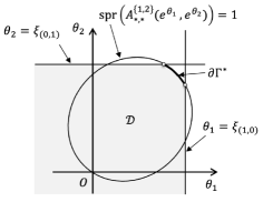
Figure 4: Domain $\mathcal{D}$ of Type 1

Define the following domains (see Fig. 4):

$$\mathcal{D}_{\boldsymbol{\varphi}}=\mbox{the interior of $\{(\theta_{1},\theta_{2})\in\mathbb{R}^{2}:\boldsymbol{\varphi}(e^{\theta_{1}},e^{\theta_{2}})<\infty$, element-wise\}},$$

$$\mathcal{D}_{0}=\{(\theta_{1},\theta_{2})\in\mathbb{R}^{2}:\theta_{1}<\xi_{(1,0)},\ \theta_{2}<\xi_{(0,1)}\},$$

$$\mathcal{D}^{\{1,2\}}=\{(\theta_{1},\theta_{2})\in\mathbb{R}^{2}:\mbox{$(\theta_{1},\theta_{2})<(\theta_{1}^{\prime},\theta_{2}^{\prime})$ for some $(\theta_{1}^{\prime},\theta_{2}^{\prime})\in\Gamma^{\{1,2\}}$}\},$$

$$\Gamma=\Gamma^{\{1,2\}}\cap\Gamma^{\{1\}}\cap\Gamma^{\{2\}}=\{(\theta_{1},\theta_{2})\in\Gamma^{\{1,2\}}:\theta_{1}<\theta_{1}^{*},\ \theta_{2}<\theta_{2}^{*}\},$$

$$\mathcal{D}=\{(\theta_{1},\theta_{2})\in\mathbb{R}^{2}:\mbox{$(\theta_{1},\theta_{2})<(\theta_{1}^{\prime},\theta_{2}^{\prime})$ for some $(\theta_{1}^{\prime},\theta_{2}^{\prime})\in\Gamma$}\},$$

where $\mathcal{D}_{0}$ is the intersection of the convergence domains of $\boldsymbol{\varphi}_{1}(e^{\theta_{1}})$ and $\boldsymbol{\varphi}_{2}(e^{\theta_{2}})$ and satisfies $\mathcal{D}\subset\mathcal{D}_{0}$. For a point set $S$, we denote by $\partial S$ the boundary of $S$. For example, $\partial\Gamma^{\{1,2\}}=\{(\theta_{1},\theta_{2})\in\mathbb{R}^{2}:A^{\{1,2\}}_{*,*}(e^{\theta_{1}},e^{\theta_{2}})=1\}$. Define a partial boundary of $\Gamma^{\{1,2\}}$, $\partial\Gamma^{*}$, as

$$\partial\Gamma^{*}=\partial\mathcal{D}^{\{1,2\}}\cap\mathcal{D}_{0}=\partial\mathcal{D}\cap\mathcal{D}_{0},$$

which is empty if the 2d-QBD process is not of Type 1 (see Fig. 4). The convergence domain $\mathcal{D}_{\boldsymbol{\varphi}}$ is given as follows.

Lemma 4.2.

$\mathcal{D}_{\boldsymbol{\varphi}}=\mathcal{D}$.

Proof.

By the definition, we have $\mathcal{D}=\mathcal{D}^{\{1,2\}}\cap\mathcal{D}_{0}$ and $\mathcal{D}_{\boldsymbol{\varphi}}\subset\mathcal{D}_{0}$. Furthermore, by Lemma 3.1 of [12], we have $\mathcal{D}\subset\mathcal{D}_{\boldsymbol{\varphi}}$. Hence, in order to prove the lemma, it suffices to prove $\mathcal{D}_{\boldsymbol{\varphi}}\subset\mathcal{D}^{\{1,2\}}$, which implies $\mathcal{D}_{\boldsymbol{\varphi}}\subset\mathcal{D}$. For every $\boldsymbol{c}^{\prime}=(c_{1}^{\prime},c_{2}^{\prime})\in\mathbb{N}^{2}$, if $(\theta_{1},\theta_{2})\in\mathcal{D}_{\boldsymbol{\varphi}}$, then we have

$$\infty>\boldsymbol{\varphi}(e^{\theta_{1}},e^{\theta_{2}})\geq\boldsymbol{\varphi}^{\boldsymbol{c}^{\prime}}(e^{c_{1}^{\prime}\theta_{1}+c_{2}^{\prime}\theta_{2}})$$

and this implies

$$c_{1}^{\prime}\theta_{1}+c_{2}^{\prime}\theta_{2}\leq\theta_{\boldsymbol{c}^{\prime}}^{max}=\sup\{c_{1}^{\prime}\theta_{1}^{\prime}+c_{2}^{\prime}\theta_{2}^{\prime}:(\theta_{1}^{\prime},\theta_{2}^{\prime})\in\Gamma^{\{1,2\}}\}.$$

Hence, in a manner similar to that used in the proof of Theorem 5.2 of [15], since $\boldsymbol{c}^{\prime}$ is arbitrary, we obtain $\mathcal{D}_{\boldsymbol{\varphi}}\subset\mathcal{D}^{\{1,2\}}$. This completes the proof. ∎

Note that the convergence domain of $\boldsymbol{\varphi}_{+}(e^{\theta_{1}},e^{\theta_{2}})$ coincides with that of $\boldsymbol{\varphi}(e^{\theta_{1}},e^{\theta_{2}})$ and it is given by $\mathcal{D}$. We define complex domains $\Omega$ and $\Omega_{0}$ as

$$\Omega=\{(z,w)\in\mathbb{C}^{2}:(\log|z|,\log|w|)\in\mathcal{D}\},$$

$$\Omega_{0}=\{(z,w)\in\mathbb{C}^{2}:(\log|z|,\log|w|)\in\mathcal{D}_{0}\},$$

where $\Omega\subset\Omega_{0}$. Define a vector function $\boldsymbol{g}(z,w)$ as

$$\boldsymbol{g}(z,w)=\boldsymbol{\varphi}_{1}(z)(A^{\{1\}}_{*,*}(z,w)-I)+\boldsymbol{\varphi}_{2}(w)(A^{\{2\}}_{*,*}(z,w)-I)+\boldsymbol{\nu}_{(0.0)}(A^{\emptyset}_{*,*}(z,w)-I).$$ (4.42)

Then, if $(z,w)\in\Omega$, series $\boldsymbol{\varphi}(z,w)$ absolutely converges element-wise and we have, by the stationary equation $\boldsymbol{\nu}P=\boldsymbol{\nu}$ (see Sectin 3.1 of [12]),

$$\boldsymbol{\varphi}_{+}(z,w)(I-A^{\{1,2\}}_{*,*}(z,w))=\boldsymbol{g}(z,w).$$ (4.43)

Using this equation, we analytically extend $\boldsymbol{\varphi}_{+}(z,w)$ outer $\Omega$. From (4.43), we obtain

$$\boldsymbol{\varphi}_{+}(z,w)=\frac{\boldsymbol{g}(z,w)\,\mbox{\rm adj}(I-A^{\{1,2\}}_{*,*}(z,w))}{\det(I-A^{\{1,2\}}_{*,*}(z,w))}.$$ (4.44)

Both the numerator and denominator of the right hand side of (4.44) are analytic in $\Omega_{0}$. Hence, by the identity theorem, $\boldsymbol{\varphi}_{+}(z,w)$ can analytically be extended over $\Omega_{0}$ and the extended $\boldsymbol{\varphi}_{+}(z,w)$ is meromorphic in $\Omega_{0}$, where zeros of $\det(I-A^{\{1,2\}}_{*,*}(z,w))$ may be poles of $\boldsymbol{\varphi}_{+}(z,w)$.

For positive real numbers $x$ and $y$, denote by $\chi^{A}(x,y)$ the maximum eigenvalue (Perron-Frobenius eigenvalue) of $A^{\{1,2\}}_{*,*}(x,y)$ and by $\boldsymbol{u}^{A}(x,y)$ and $\boldsymbol{v}^{A}(x,y)$ the left and right eigenvectors with respect to the eigenvalue, respectively, satisfying $\boldsymbol{u}^{A}(x,y)\boldsymbol{v}^{A}(x,y)=1$. Since $A^{\{1,2\}}_{*,*}(x,y)$ is irreducible, the eigenvalue $\chi^{A}(x,y)$ is simple and the eigenvectors $\boldsymbol{u}^{A}(x,y)$ and $\boldsymbol{v}^{A}(x,y)$ are positive. The vector function $\boldsymbol{g}(z,w)$ satisfies the following property.

Proposition 4.11.

For every $(\theta_{1},\theta_{2})\in\partial\Gamma^{*}$, $\boldsymbol{g}(e^{\theta_{1}},e^{\theta_{2}})\boldsymbol{v}^{A}(e^{\theta_{1}},e^{\theta_{2}})>0$.

Proof.

Assume Type 1 and let $(\theta_{1},\theta_{2})$ be an arbitrary point on $\partial\Gamma^{*}$. Set $w=e^{\theta_{2}}$. Then, each element of $\boldsymbol{\varphi}_{+}(z,e^{\theta_{2}})$ is a function of one variable, and it is meromorphic in $\Delta_{e^{\xi_{(1,0)}}}\setminus\{0\}$. Furthermore, the point $z=e^{\theta_{1}}$ is a pole of it since the convergence domain of $\boldsymbol{\varphi}_{+}(e^{\theta_{1}^{\prime}},e^{\theta_{2}^{\prime}})$ is $\mathcal{D}$ and $\partial\Gamma^{*}\subset\partial\mathcal{D}$. Define a function $f(\lambda,z,w)$ as $f(\lambda,z,w)=\det(\lambda I-A^{\{1,2\}}_{*,*}(z,w))$, and $f_{\lambda}(\lambda,z,w)$ and $f_{z}(\lambda,z,w)$ as $f_{\lambda}(\lambda,z,w)=\frac{\partial}{\partial\lambda}f(\lambda,z,w)$ and $f_{z}(\lambda,z,w)=\frac{\partial}{\partial z}f(\lambda,z,w)$, respectively. For positive numbers $x$ and $y$, since $A^{\{1,2\}}_{*,*}(x,y)$ is irreducible, the eigenvalue $\chi^{A}(x,y)$ is simple and differentiable in $x$ and $y$. Define $\chi^{A}_{x}(x,y)$ as $\chi^{A}_{x}(x,y)=\frac{\partial}{\partial x}\chi^{A}(x,y)$. By Corollary 2 of [17], we have

$$\mbox{\rm adj}(I-A^{\{1,2\}}_{*,*}(e^{\theta_{1}},e^{\theta_{2}}))=f_{\lambda}(1,e^{\theta_{1}},e^{\theta_{2}})\boldsymbol{v}^{A}(e^{\theta_{1}},e^{\theta_{2}})\boldsymbol{u}^{A}(e^{\theta_{1}},e^{\theta_{2}}).$$ (4.45)

In a manner similar to that used in the proof of Proposition 5.3 of [12], we obtain

$$\lim_{x\uparrow e^{\theta_{1}}}(e^{\theta_{1}}-x)^{-1}f(1,x,e^{\theta_{2}})=\chi^{A}_{x}(e^{\theta_{1}},e^{\theta_{2}})f_{\lambda}(1,e^{\theta_{1}},e^{\theta_{2}}),$$ (4.46)

where $\chi^{A}_{x}(e^{\theta_{1}},e^{\theta_{2}})$ is positive since $\chi^{A}(e^{\theta_{1}^{\prime}},e^{\theta_{2}^{\prime}})$ is convex in $(\theta_{1}^{\prime},\theta_{2}^{\prime})$ and, under Assumption 2.5,

$$\chi^{A}(e^{\theta_{1}},e^{\theta_{2}})=1>\min_{(\theta_{1}^{\prime},\theta_{2}^{\prime})\in\Gamma^{\{1,2\}}}\chi^{A}(e^{\theta_{1}^{\prime}},e^{\theta_{2}^{\prime}}).$$

Hence, by (4.44), we obtain,

$$\lim_{x\uparrow e^{\theta_{1}}}(e^{\theta_{1}}-x)\boldsymbol{\varphi}_{+}(x,e^{\theta_{2}})=\chi^{A}_{x}(e^{\theta_{1}},e^{\theta_{2}})^{-1}\boldsymbol{g}(e^{\theta_{1}},e^{\theta_{2}})\boldsymbol{v}^{A}(e^{\theta_{1}},e^{\theta_{2}})\boldsymbol{u}^{A}(e^{\theta_{1}},e^{\theta_{2}}),$$ (4.47)

where $\chi^{A}_{x}(e^{\theta_{1}},e^{\theta_{2}})$ and $\boldsymbol{u}^{A}(e^{\theta_{1}},e^{\theta_{2}})$ are positive. Since the point $z=e^{\theta_{1}}$ is a zero of $f(1,z,e^{\theta_{2}})$ with order one, if $\boldsymbol{g}(e^{\theta_{1}},e^{\theta_{2}})\boldsymbol{v}^{A}(e^{\theta_{1}},e^{\theta_{2}})=0$, the point $z=e^{\theta_{1}}$ becomes a removable singularity of each element of $\boldsymbol{\varphi}_{+}(z,e^{\theta_{2}})$, and this contradicts that the point $z=e^{\theta_{1}}$ is a pole of each element of $\boldsymbol{\varphi}_{+}(z,e^{\theta_{2}})$. Hence, we have $\boldsymbol{g}(e^{\theta_{1}},e^{\theta_{2}})\boldsymbol{v}^{A}(e^{\theta_{1}},e^{\theta_{2}})>0$. ∎

Denote $\eta_{\boldsymbol{c},1}^{max}=\eta^{R}_{\boldsymbol{c},1}(\theta_{\boldsymbol{c}}^{max})$ and $\eta_{\boldsymbol{c},2}^{max}=\eta^{R}_{\boldsymbol{c},2}(\theta_{\boldsymbol{c}}^{max})$. Since $\boldsymbol{c}=(1,1)$, they satisfy $\theta_{\boldsymbol{c}}^{max}=\eta_{\boldsymbol{c},1}^{max}+\eta_{\boldsymbol{c},2}^{max}$. The limit of $\Phi^{\boldsymbol{c}}_{\boldsymbol{x},*}(z)$ is given as follows.

Proposition 4.12.

Let $\boldsymbol{x}=(x_{1},x_{2})$ be an arbitrary point in $\mathbb{Z}_{+}^{2}$. Then, the matrix function $\Phi^{\boldsymbol{c}}_{\boldsymbol{x},*}(z)$ satisfies, for a positive row vector $\boldsymbol{u}_{\boldsymbol{c}}$,

$$\lim_{\tilde{\Delta}_{e^{\theta_{\boldsymbol{c}}^{max}}}\ni z\to e^{\theta_{\boldsymbol{c}}^{max}}}(e^{\theta_{\boldsymbol{c}}^{max}}-z)^{\frac{1}{2}}\Phi^{\boldsymbol{c}}_{(x_{1},x_{2}),*}(z)$$ (4.48)

$$\qquad\qquad\qquad=\hat{g}^{\Phi}e^{x_{1}\eta_{\boldsymbol{c},1}^{max}+x_{2}\eta_{\boldsymbol{c},2}^{max}}\boldsymbol{v}^{A}(e^{\eta_{\boldsymbol{c},1}^{max}},e^{\eta_{\boldsymbol{c},2}^{max}})\boldsymbol{u}_{\boldsymbol{c}}>O,$$ (4.49)

where the positive constant $\hat{g}^{\Phi}$ is given by (4.24).

Proof.

By (4.14) and (4.23), we obtain that, for every $\boldsymbol{x}=(x_{1},x_{2})\in\mathbb{Z}_{+}^{2}$,

$$\lim_{\tilde{\Delta}_{e^{\theta_{\boldsymbol{c}}^{max}}}\ni z\to e^{\theta_{\boldsymbol{c}}^{max}}}(e^{\theta_{\boldsymbol{c}}^{max}}-z)^{\frac{1}{2}}\hat{\Phi}_{(x_{1},x_{2}),*}(z)=\hat{g}^{\Phi}(e^{\theta_{\boldsymbol{c}}^{max}})^{x_{1}}\hat{G}_{0,*}(e^{\theta_{\boldsymbol{c}}^{max}})^{x_{2}}\hat{\boldsymbol{v}}^{U}(e^{\theta_{\boldsymbol{c}}^{max}})\hat{\boldsymbol{u}}^{U}(e^{\theta_{\boldsymbol{c}}^{max}}).$$ (4.50)

By the proof of Proposition 4.6, $\hat{\boldsymbol{v}}^{U}(e^{\theta_{\boldsymbol{c}}^{max}})$ is also the left eigenvector of $\hat{G}_{0,*}(e^{\theta_{\boldsymbol{c}}^{max}})$, satisfying $\hat{G}_{0,*}(e^{\theta_{\boldsymbol{c}}^{max}})\hat{\boldsymbol{v}}^{U}(e^{\theta_{\boldsymbol{c}}^{max}})=e^{2\eta_{\boldsymbol{c},2}^{max}}\hat{\boldsymbol{v}}^{U}(e^{\theta_{\boldsymbol{c}}^{max}})$. Since $e^{\theta_{\boldsymbol{c}}^{max}}=e^{\eta_{\boldsymbol{c},1}^{max}+\eta_{\boldsymbol{c},2}^{max}}$, we have

$$\lim_{\tilde{\Delta}_{e^{\theta_{\boldsymbol{c}}^{max}}}\ni z\to e^{\theta_{\boldsymbol{c}}^{max}}}(e^{\theta_{\boldsymbol{c}}^{max}}-z)^{\frac{1}{2}}\hat{\Phi}_{(x_{1},x_{2}),*}(z)=\hat{g}^{\Phi}e^{\eta_{\boldsymbol{c},1}^{max}x_{1}+\eta_{\boldsymbol{c},2}^{max}(x_{1}+2x_{2})}\hat{\boldsymbol{v}}^{U}(e^{\theta_{\boldsymbol{c}}^{max}})\hat{\boldsymbol{u}}^{U}(e^{\theta_{\boldsymbol{c}}^{max}}).$$ (4.51)

Denote $\hat{\boldsymbol{u}}^{U}(e^{\theta_{\boldsymbol{c}}^{max}})=\begin{pmatrix}\boldsymbol{u}_{1}&\boldsymbol{u}_{2}\end{pmatrix}$ and $\hat{\boldsymbol{v}}^{U}(e^{\theta_{\boldsymbol{c}}^{max}})=\begin{pmatrix}\boldsymbol{v}_{1}\cr\boldsymbol{v}_{2}\end{pmatrix}$, respectively. By (4.11) and (4.51), setting $\boldsymbol{x}=(0,0)$, we obtain

$$\lim_{\tilde{\Delta}_{e^{\theta_{\boldsymbol{c}}^{max}}}\ni z\to e^{\theta_{\boldsymbol{c}}^{max}}}(e^{\theta_{\boldsymbol{c}}^{max}}-z)^{\frac{1}{2}}\begin{pmatrix}\Phi^{\boldsymbol{c}}_{(0,0),*}(z)&\Phi^{\boldsymbol{c}}_{(0,-1),*}(z)\cr\Phi^{\boldsymbol{c}}_{(0,1),*}(z)&\Phi^{\boldsymbol{c}}_{(0,0),*}(z)\end{pmatrix}=\hat{g}^{\Phi}\begin{pmatrix}\boldsymbol{v}_{1}\boldsymbol{u}_{1}&\boldsymbol{v}_{1}\boldsymbol{u}_{2}\cr\boldsymbol{v}_{2}\boldsymbol{u}_{1}&\boldsymbol{v}_{2}\boldsymbol{u}_{2}\end{pmatrix}.$$ (4.52)

Hence, we have $\boldsymbol{v}_{1}\boldsymbol{u}_{1}=\boldsymbol{v}_{2}\boldsymbol{u}_{2}$, and this leads us to $\boldsymbol{v}_{2}=c\boldsymbol{v}_{1}$ and $\boldsymbol{u}_{2}=c^{-1}\boldsymbol{u}_{1}$, where $c=\boldsymbol{u}_{1}\boldsymbol{v}_{2}/(\boldsymbol{u}_{2}\boldsymbol{v}_{2})$. Analogously, by (4.11) and (4.51), setting $\boldsymbol{x}=(0,1)$, we obtain $e^{2\eta_{\boldsymbol{c},2}^{max}}\boldsymbol{v}_{1}\boldsymbol{u}_{2}=\boldsymbol{v}_{2}\boldsymbol{u}_{1}$, and this leads us to $c=e^{\eta_{\boldsymbol{c},2}^{max}}$. As a result, by (4.11) and (4.51), we have, for every $\boldsymbol{x}=(x_{1},x_{2})\in\mathbb{Z}_{+}^{2}$,

$$\lim_{\tilde{\Delta}_{e^{\theta_{\boldsymbol{c}}^{max}}}\ni z\to e^{\theta_{\boldsymbol{c}}^{max}}}(e^{\theta_{\boldsymbol{c}}^{max}}-z)^{\frac{1}{2}}\Phi^{\boldsymbol{c}}_{(x_{1},x_{1}+2x_{2}),*}(z)=\hat{g}^{\Phi}e^{\eta_{\boldsymbol{c},1}^{max}x_{1}+\eta_{\boldsymbol{c},2}^{max}(x_{1}+2x_{2})}\boldsymbol{v}_{1}\boldsymbol{u}_{1},$$ (4.53)

$$\lim_{\tilde{\Delta}_{e^{\theta_{\boldsymbol{c}}^{max}}}\ni z\to e^{\theta_{\boldsymbol{c}}^{max}}}(e^{\theta_{\boldsymbol{c}}^{max}}-z)^{\frac{1}{2}}\Phi^{\boldsymbol{c}}_{(x_{1},x_{1}+2x_{2}+1),*}(z)=\hat{g}^{\Phi}e^{\eta_{\boldsymbol{c},1}^{max}x_{1}+\eta_{\boldsymbol{c},2}^{max}(x_{1}+2x_{2}+1)}\boldsymbol{v}_{1}\boldsymbol{u}_{1}.$$ (4.54)

Since, in (4.53) and (4.54), $x_{1}$ and $x_{2}$ are arbitrary, the same result holds for $\Phi^{\boldsymbol{c}}_{(x_{1}^{\prime},x_{2}^{\prime}),*}(z)$, where $x_{1}^{\prime}$ and $x_{2}^{\prime}$ are nonnegative integers. Furthermore, we see that $\boldsymbol{u}_{\boldsymbol{c}}$ in (4.49) is given by $\boldsymbol{u}_{1}$.

We identify $\boldsymbol{v}_{1}$. Define matrix functions:

$$B_{-2}(z)=A_{1,-1}z,\quad B_{-1}(z)=A_{0,-1}+A_{1,0}z,\quad B_{0}(z)=A_{-1,-1}z^{-1}+A_{0,0}+A_{1,1}z,$$

$$B_{1}(z)=A_{-1,0}z^{-1}+A_{0,1},\quad B_{2}(z)=A_{-1,1}z^{-1},$$

and

$$B_{*}(z,w)=\sum_{j=-2}^{2}B_{j}(z)w^{j},$$

where we have the following (see Section 3 of [14]):

$$B_{*}(e^{\theta_{1}},e^{\theta_{2}})=A^{\{1,2\}}_{*,*}(e^{\theta_{1}-\theta_{2}},e^{\theta_{2}}).$$ (4.55)

By Remark 2.4 of [15], if $\hat{\boldsymbol{v}}=\begin{pmatrix}\hat{\boldsymbol{v}}_{1}\cr\hat{\boldsymbol{v}}_{2}\end{pmatrix}$ is the right eigenvector of $\hat{A}^{\{1,2\}}_{*,*}(e^{\theta_{1}},e^{\theta_{2}})$ with respect to eigenvalue $\lambda$, then $\hat{\boldsymbol{v}}_{2}=e^{\theta_{2}/2}\hat{\boldsymbol{v}}_{1}$ and $\hat{\boldsymbol{v}}_{1}$ is the right eigenvector of $B_{*}(e^{\theta_{1}},e^{\theta_{2}/2})$ with respect to the eigenvalue $\lambda$, and vice versa. By the proof of Proposition 4.6, we already know that $\hat{\boldsymbol{v}}^{U}(e^{\theta_{\boldsymbol{c}}^{max}})$ is the right eigenvector of $\hat{A}^{\{1,2\}}_{*,*}(e^{\theta_{\boldsymbol{c}}^{max}},e^{2\eta_{\boldsymbol{c},2}^{max}})$ with respect to the eigenvalue $1$. Hence, we have

$$\boldsymbol{v}_{1}=B_{*}(e^{\theta_{\boldsymbol{c}}^{max}},e^{\eta_{\boldsymbol{c},2}^{max}})\boldsymbol{v}_{1}=A^{\{1,2\}}_{*,*}(e^{\eta_{\boldsymbol{c},1}^{max}},e^{\eta_{\boldsymbol{c},2}^{max}})\boldsymbol{v}_{1}.$$ (4.56)

This implies $\boldsymbol{v}_{1}=\boldsymbol{v}^{A}(e^{\eta_{\boldsymbol{c},1}^{max}},e^{\eta_{\boldsymbol{c},2}^{max}})$. ∎

The coefficient vector $\boldsymbol{\varphi}^{\boldsymbol{c}}_{1,-1}$ in the Puiseux series of $\boldsymbol{\varphi}^{\boldsymbol{c}}(z)$ is given as follows.

Proof of Proposition 4.3.

Assume Type 1. If $\bar{\eta}_{1}^{\prime}(\theta_{2}^{*})<-c_{1}/c_{2}=-1<1/\bar{\eta}_{2}^{\prime}(\theta_{1}^{*})$, $\boldsymbol{\varphi}_{1}(z)$ element-wise converges at $z=e^{\eta_{\boldsymbol{c},1}^{max}}<e^{\xi_{(1,0)}}$ and $\boldsymbol{\varphi}_{2}(w)$ at $w=e^{\eta_{\boldsymbol{c},2}^{max}}<e^{\xi_{(0,1)}}$. Hence, applying (4.49) to expression (4.7) of $\boldsymbol{\varphi}^{\boldsymbol{c}}(z)$, we obtain, for a positive row vector $\boldsymbol{u}_{\boldsymbol{c}}$,

$$\boldsymbol{\varphi}^{\boldsymbol{c}}_{1,-1}=\lim_{\tilde{\Delta}_{e^{\theta_{\boldsymbol{c}}^{max}}}\ni z\to e^{\theta_{\boldsymbol{c}}^{max}}}(e^{\theta_{\boldsymbol{c}}^{max}}-z)^{\frac{1}{2}}\boldsymbol{\varphi}^{\boldsymbol{c}}(z)=\hat{g}^{\Phi}\boldsymbol{g}(e^{\eta_{\boldsymbol{c},1}^{max}},e^{\eta_{\boldsymbol{c},2}^{max}})\boldsymbol{v}^{A}(e^{\eta_{\boldsymbol{c},1}^{max}},e^{\eta_{\boldsymbol{c},2}^{max}})\boldsymbol{u}_{\boldsymbol{c}},$$ (4.57)

where $\boldsymbol{u}_{\boldsymbol{c}}$ is given by $\boldsymbol{u}_{1}$ in the proof of Proposition 4.12. The row vector $\boldsymbol{u}_{0}^{\boldsymbol{c}}$ in Proposition 4.3 is given by the right hand side of (4.57), which is positive since $\boldsymbol{g}(e^{\eta_{\boldsymbol{c},1}^{max}},e^{\eta_{\boldsymbol{c},2}^{max}})\boldsymbol{v}^{A}(e^{\eta_{\boldsymbol{c},1}^{max}},e^{\eta_{\boldsymbol{c},2}^{max}})>0$ by Proposition 4.11. ∎

4.4 Proof of Corollary 2.1

Define a probability distribution $\tilde{\boldsymbol{\nu}}=(\tilde{\boldsymbol{\nu}}_{\boldsymbol{x}},\boldsymbol{x}\in\mathbb{Z}^{2})$ on $\mathbb{Z}^{2}\times S_{0}$ as

$$\tilde{\boldsymbol{\nu}}_{\boldsymbol{x}}=\left\{\begin{array}[]{ll}\boldsymbol{\nu}_{\boldsymbol{x}},&\boldsymbol{x}\in\mathbb{Z}_{+}^{2},\cr\mathbf{0}^{\top},&\mbox{otherwise}.\end{array}\right.$$

This $\tilde{\boldsymbol{\nu}}$ is the stationary distribution of a certain Markov chain on the state space $\mathbb{Z}^{2}\times S_{0}$, see Section 2.2 of [16]. For $\boldsymbol{x}\in\mathbb{Z}^{2}$, the expression of $\tilde{\boldsymbol{\nu}}_{\boldsymbol{x}}$ is given by (2.8) of [16]. For $\boldsymbol{c}\in\mathbb{N}^{2}$ and $\boldsymbol{x},\boldsymbol{x}^{\prime}\in\mathbb{Z}^{2}$, define a vector generating function $\bar{\boldsymbol{\varphi}}^{\boldsymbol{c}}_{\boldsymbol{x}}$ and matrix generating function $\Phi^{\boldsymbol{c}}_{\boldsymbol{x}^{\prime},*+\boldsymbol{x}}(z)$ as

$$\bar{\boldsymbol{\varphi}}^{\boldsymbol{c}}_{\boldsymbol{x}}(z)=\sum_{k=-\infty}^{\infty}z^{k}\tilde{\boldsymbol{\nu}}_{k\boldsymbol{c}+\boldsymbol{x}},\quad\Phi^{\boldsymbol{c}}_{\boldsymbol{x}^{\prime},*+\boldsymbol{x}}(z)=\sum_{k=-\infty}^{\infty}z^{k}\Phi^{\{1,2\}}_{\boldsymbol{x}^{\prime},k\boldsymbol{c}+\boldsymbol{x}}.$$

Since $\Phi^{\{1,2\}}_{\boldsymbol{x}^{\prime},k\boldsymbol{c}+\boldsymbol{x}}=\Phi^{\{1,2\}}_{\boldsymbol{x}^{\prime}-\boldsymbol{x},k\boldsymbol{c}}$, we have $\Phi^{\boldsymbol{c}}_{\boldsymbol{x}^{\prime},*+\boldsymbol{x}}(z)=\Phi^{\boldsymbol{c}}_{\boldsymbol{x}^{\prime}-\boldsymbol{x},*}(z)$. Hence, by (2.8) of [16], we have

$$\bar{\boldsymbol{\varphi}}^{\boldsymbol{c}}_{\boldsymbol{x}}(z)=\bar{\boldsymbol{\varphi}}^{\boldsymbol{c}}_{0,\boldsymbol{x}}(z)+\bar{\boldsymbol{\varphi}}^{\boldsymbol{c}}_{1,\boldsymbol{x}}(z)+\bar{\boldsymbol{\varphi}}^{\boldsymbol{c}}_{2,\boldsymbol{x}}(z),$$ (4.58)

where

$$\bar{\boldsymbol{\varphi}}^{\boldsymbol{c}}_{0,\boldsymbol{x}}(z)=\sum_{i_{1},i_{2}\in\{-1,0,1\}}\boldsymbol{\nu}_{(0,0)}(A^{\emptyset}_{i_{1},i_{2}}-A^{\{1,2\}}_{i_{1},i_{2}})\Phi^{\boldsymbol{c}}_{(i_{1},i_{2})-\boldsymbol{x},*}(z),$$ (4.59)

$$\bar{\boldsymbol{\varphi}}^{\boldsymbol{c}}_{1,\boldsymbol{x}}(z)=\sum_{k=1}^{\infty}\ \sum_{i_{1},i_{2}\in\{-1,0,1\}}\boldsymbol{\nu}_{(k,0)}(A^{\{1\}}_{i_{1},i_{2}}-A^{\{1,2\}}_{i_{1},i_{2}})\Phi^{\boldsymbol{c}}_{(k+i_{1},i_{2})-\boldsymbol{x},*}(z),$$ (4.60)

$$\bar{\boldsymbol{\varphi}}^{\boldsymbol{c}}_{2,\boldsymbol{x}}(z)=\sum_{k=1}^{\infty}\ \sum_{i_{1},i_{2}\in\{-1,0,1\}}\boldsymbol{\nu}_{(0,k)}(A^{\{2\}}_{i_{1},i_{2}}-A^{\{1,2\}}_{i_{1},i_{2}})\Phi^{\boldsymbol{c}}_{(i_{1},k+i_{2})-\boldsymbol{x},*}(z).$$ (4.61)

For $\boldsymbol{c}\in\mathbb{N}^{2}$ and $\boldsymbol{x}\in\mathbb{Z}_{+}^{2}$, define the vector generating function $\boldsymbol{\varphi}^{\boldsymbol{c}}_{\boldsymbol{x}}(z)$ of vector sequence $\{\boldsymbol{\nu}_{k\boldsymbol{c}+\boldsymbol{x}}:k\in\mathbb{Z}_{+}\}$ as

$$\boldsymbol{\varphi}^{\boldsymbol{c}}_{\boldsymbol{x}}(z)=\sum_{k=0}^{\infty}z^{k}\boldsymbol{\nu}_{k\boldsymbol{c}+\boldsymbol{x}}.$$

The asymptotic decay function of the sequence $\{\boldsymbol{\nu}_{k\boldsymbol{c}+\boldsymbol{x}}:k\in\mathbb{Z}_{+}\}$ is obtained through the analytic property of the vector function $\boldsymbol{\varphi}^{\boldsymbol{c}}_{\boldsymbol{x}}(z)$.

Proof of Corollary 2.1.

Assume $\boldsymbol{c}=(1,1)$. Let $\boldsymbol{x}=(x_{1},x_{2})$ be a point in $\mathbb{Z}_{+}^{2}$ and set $k_{0}=\max\{x_{1},x_{2}\}$, then $\boldsymbol{x}-k_{0}\boldsymbol{c}\leq\mathbf{0}$. We have

$$\bar{\boldsymbol{\varphi}}^{\boldsymbol{c}}_{\boldsymbol{x}-k_{0}\boldsymbol{c}}(z)=\sum_{k=-\infty}^{\infty}z^{k}\tilde{\boldsymbol{\nu}}_{k\boldsymbol{c}+\boldsymbol{x}-k_{0}\boldsymbol{c}}=\sum_{k=-\min\{x_{1},x_{2}\}}^{-1}z^{k+k_{0}}\boldsymbol{\nu}_{k\boldsymbol{c}+\boldsymbol{x}}+z^{k_{0}}\boldsymbol{\varphi}^{\boldsymbol{c}}_{\boldsymbol{x}}(z).$$ (4.62)

Since the first term and function $z^{k_{0}}$ on the right hand side of (4.62) are analytic in $\mathbb{C}$, the analytic property of the vector function $\boldsymbol{\varphi}^{\boldsymbol{c}}_{\boldsymbol{x}}(z)$ coincides with that of $\bar{\boldsymbol{\varphi}}^{\boldsymbol{c}}_{\boldsymbol{x}-k_{0}\boldsymbol{c}}(z)$. Furthermore, $\bar{\boldsymbol{\varphi}}^{\boldsymbol{c}}_{\boldsymbol{x}-k_{0}\boldsymbol{c}}(z)$ is given by (4.62) and we have

$$\hat{\Phi}^{\boldsymbol{c}}_{(i_{1},k+i_{2})-(\boldsymbol{x}-k_{0}\boldsymbol{c}),*}(z)=(z^{i_{1}}\hat{G}_{0,*}(z)^{k+i_{2}})(z^{k_{0}-x_{1}}\hat{G}_{0,*}(z)^{k_{0}-x_{2}})\hat{\Phi}_{(0,0),*}(z),$$

where $k_{0}-x_{1}\geq 0$ and $k_{0}-x_{2}\geq 0$. Hence, in a manner similar to that used for the vector function $\boldsymbol{\varphi}^{\boldsymbol{c}}(z)$, we see that the vector function $\bar{\boldsymbol{\varphi}}^{\boldsymbol{c}}_{\boldsymbol{x}-k_{0}\boldsymbol{c}}(z)$ is analytic in $\Delta_{e^{\xi_{\boldsymbol{c}}}}\cup\partial\Delta_{e^{\xi_{\boldsymbol{c}}}}\setminus\{e^{\xi_{\boldsymbol{c}}}\}$ and its singularity at the point $e^{\xi_{\boldsymbol{c}}}$ coincides with that of $\boldsymbol{\varphi}^{\boldsymbol{c}}(z)$. For a general direction vector $\boldsymbol{c}\in\mathbb{N}^{2}$, we can also see that the same results hold true for $\bar{\boldsymbol{\varphi}}^{\boldsymbol{c}}_{\boldsymbol{x}-k_{0}\boldsymbol{c}}(z)$ by using the block state process derived from the original 2d-QBD process; See Section 3.3 of [16]. This completes the proof. ∎

5 Concluding remark

Here we consider a topic with respect to an occupation measure. Recall that $P^{\{1,2\}}=(P^{\{1,2\}}_{\boldsymbol{x},\boldsymbol{x}^{\prime}};\boldsymbol{x},\boldsymbol{x}^{\prime}\in\mathbb{Z}^{2})$ is the transition probability matrix of the induced MA-process $\{\boldsymbol{Y}^{\{1,2\}}_{n}\}$ and $\Phi^{\{1,2\}}=(\Phi^{\{1,2\}}_{\boldsymbol{x},\boldsymbol{x}^{\prime}};\boldsymbol{x},\boldsymbol{x}^{\prime}\in\mathbb{Z}^{2})$ the fundamental matrix of $P^{\{1,2\}}$. Let $h_{\boldsymbol{c}}^{\Phi}(k)$ be the asymptotic decay function of the matrix sequence $\{\Phi^{\{1,2\}}_{\boldsymbol{x},k\boldsymbol{c}};k\in\mathbb{N}\}$, i.e., for some positive matrix $C_{\boldsymbol{x}}$,

$$\lim_{k\to\infty}\Phi^{\{1,2\}}_{\boldsymbol{x},k\boldsymbol{c}}/h_{\boldsymbol{c}}^{\Phi}(k)=C_{\boldsymbol{x}}.$$ (5.1)

By using the block state process derived from the original 2d-QBD process, we can see that Proposition 4.1 also holds for every direction vector $\boldsymbol{c}$ in $\mathbb{N}^{2}$. Hence, we obtain

$$h_{\boldsymbol{c}}^{\Phi}(k)=k^{-\frac{1}{2}}e^{-\theta_{\boldsymbol{c}}^{max}k}.$$ (5.2)

Furthermore, recall that $P^{+}$ is a partial matrix of $P^{\{1,2\}}$ given by restricting the state space of the additive part to the positive quadrant, i.e., $P^{+}=(P^{\{1,2\}}_{\boldsymbol{x},\boldsymbol{x}^{\prime}};\boldsymbol{x},\boldsymbol{x}^{\prime}\in\mathbb{N}^{2})$. $P^{+}$ is also a partial matrix of the transition probability matrix of the original 2d-QBD process, $P=(P_{\boldsymbol{x},\boldsymbol{x}^{\prime}};\boldsymbol{x},\boldsymbol{x}^{\prime}\in\mathbb{Z}_{+}^{2})$, i.e., $P^{+}=(P_{\boldsymbol{x},\boldsymbol{x}^{\prime}};\boldsymbol{x},\boldsymbol{x}^{\prime}\in\mathbb{N}^{2})$. Let $\tilde{Q}=(\tilde{Q}_{\boldsymbol{x},\boldsymbol{x}^{\prime}};\boldsymbol{x},\boldsymbol{x}^{\prime}\in\mathbb{N}^{2})$ be the fundamental matrix of $P^{+}$, i.e., $\tilde{Q}=\sum_{n=0}^{\infty}(P^{+})^{n}$. For $j,j^{\prime}\in S_{0}$, denote by $\tilde{q}_{(\boldsymbol{x},j),(\boldsymbol{x}^{\prime},j^{\prime})}$ the $(j,j^{\prime})$-entry of $\tilde{Q}_{\boldsymbol{x},\boldsymbol{x}^{\prime}}$. The entries of $\tilde{Q}$ are called an occupation measure in [15]. By Theorem 5.1 of [15], the asymptotic decay rate of the matrix sequence $\{\tilde{Q}_{\boldsymbol{x},k\boldsymbol{c}};k\in\mathbb{N}\}$ is given by $e^{\theta_{\boldsymbol{c}}^{max}}$, i.e.,

$$-\lim_{k\to\infty}\frac{1}{k}\log\tilde{q}_{(\boldsymbol{x},j),(k\boldsymbol{c},j^{\prime})}=\theta_{\boldsymbol{c}}^{max},$$ (5.3)

which coincides with that of the matrix sequence $\{\Phi^{\{1,2\}}_{\boldsymbol{x},k\boldsymbol{c}};k\in\mathbb{N}\}$. One question, therefore, arises: Does the asymptotic decay function of the matrix sequence $\{\tilde{Q}_{\boldsymbol{x},k\boldsymbol{c}};k\in\mathbb{N}\}$ coincide with that of the matrix sequence $\{\Phi^{\{1,2\}}_{\boldsymbol{x},k\boldsymbol{c}};k\in\mathbb{N}\}$? The answer to the question seems not to be so obvious.

Appendix A Proof of Theorem 3.1

First, we give the generalized eigenvectors of $G(z)$ for $z\in\Delta_{e^{\theta_{1}^{min}},e^{\theta_{1}^{max}}}\setminus\mathcal{E}_{1}$, then analytically extend them to $z\in\mathbb{C}\setminus\mathcal{E}_{1}$. Set $\Omega=\Delta_{e^{\theta_{1}^{min}},e^{\theta_{1}^{max}}}\setminus(\mathcal{E}_{1}\cup\mathcal{E}_{2})$.

For each $k\in\{1,2,...,m_{0}\}$ and for each $z\in\Omega\setminus\bigcup_{k=1}^{m_{0}}\mathcal{E}^{G}_{k}$, since the Jordan normal form of $G(z)$ is given by (3.4), there exist linearly independent vectors called the generalized eigenvectors of $G(z)$ with respect to the eigenvalue $\check{\alpha}_{k}(z)$, $\check{\boldsymbol{v}}_{k,i,j}(z),\,i=1,2,...,m_{k,0},\,j=1,2,...,m_{k,i},$ satisfying

$$(\check{\alpha}_{k}(z)I-G(z))\check{\boldsymbol{v}}_{k,i,j}(z)=\check{\boldsymbol{v}}_{k,i,j+1}(z),$$ (A.1)

where $\check{\boldsymbol{v}}_{k,i,m_{k,i}+1}(z)=\mathbf{0}$. For each $i$, $\check{\boldsymbol{v}}_{k,i,j}(z),\,j=1,2,...,m_{k,i},$ are called a Jordan sequence of the generalized eigenvectors. Using the Jordan sequences, we define $l_{\check{q}(k)}\times 1$ block vectors, $\boldsymbol{v}_{k,i,j}(z),\,i=1,2,...,m_{k,0},\,j=1,2,...,m_{k,i},$ as

$$\boldsymbol{v}_{k,i,j}(z)=\mbox{\rm vec}\!\begin{pmatrix}\check{\boldsymbol{v}}_{k,i,j}(z)&\check{\boldsymbol{v}}_{k,i,j+1}(z)&\cdots&\check{\boldsymbol{v}}_{k,i,m_{k,i}}(z)&\mathbf{0}&\cdots&\mathbf{0}\end{pmatrix},$$

where, for a matrix $A=\begin{pmatrix}\boldsymbol{a}_{1}&\boldsymbol{a}_{2}&\cdots&\boldsymbol{a}_{n}\end{pmatrix}$, $\mbox{\rm vec}(A)$ is the column vector given by

$$\mbox{\rm vec}(A)=\begin{pmatrix}\boldsymbol{a}_{1}\cr\boldsymbol{a}_{2}\cr\vdots\cr\boldsymbol{a}_{n}\end{pmatrix}.$$

We also define a vector space $\mathbb{V}^{G}_{k}(z)$ as

$$\mathbb{V}^{G}_{k}(z)=\mathrm{span}\,\{\boldsymbol{v}_{k,i,j}(z):i=1,2,...,m_{k,0},\,j=1,2,...,m_{k,i}\}.$$

Note that the generalized eigenvectors $\check{\boldsymbol{v}}_{k,i,j}(z)$ are not unique but $\mathbb{V}^{G}_{k}(z)$ is. Since the generalized eigenvectors are linearly independent, $\boldsymbol{v}_{k,i,j}(z)$ are also linearly independent and we have

$$\dim\mathbb{V}^{G}_{k}(z)=\sum_{i=1}^{m_{k,0}}m_{k,i}=l_{\check{q}(k)}.$$

For $k\in\{1,2,...,m_{0}\}$, define an $l_{\check{q}(k)}\times l_{\check{q}(k)}$ block matrix function $\Lambda^{G}_{k}(z)$ as

$$\Lambda^{G}_{k}(z)=\begin{pmatrix}\check{\alpha}_{k}(z)I-G(z)&-I&\cr&\check{\alpha}_{k}(z)I-G(z)&-I&\cr&\qquad\qquad\quad\ddots&\qquad\qquad\quad\ddots&\cr&&\check{\alpha}_{k}(z)I-G(z)&-I\cr&&&\check{\alpha}_{k}(z)I-G(z)\end{pmatrix}.$$

We give the following proposition.

Proposition A.1.

For each $k\in\{1,2,...,m_{0}\}$ and for each $z\in\Omega\setminus\bigcup_{k=1}^{m_{0}}\mathcal{E}^{G}_{k}$,

$$\mathrm{Ker}\,\Lambda^{G}_{k}(z)=\mathbb{V}^{G}_{k}(z).$$ (A.2)

Proof.

Assume $\boldsymbol{v}\in\mathbb{V}^{G}_{k}(z)$. Then, by the definition of $\mathbb{V}^{G}_{k}(z)$, we have $\Lambda^{G}_{k}(z)\boldsymbol{v}=\mathbf{0}$ and $\boldsymbol{v}\in\mathrm{Ker}\,\Lambda^{G}_{k}(z)$. For $\boldsymbol{v}=\mbox{\rm vec}\begin{pmatrix}\boldsymbol{v}_{1}&\boldsymbol{v}_{2}&\cdots&\boldsymbol{v}_{l_{\check{q}(k)}}\end{pmatrix}$, assume $\Lambda^{G}_{k}(z)\boldsymbol{v}=\mathbf{0}$. If there exists an index $i$ such that $\boldsymbol{v}_{i}=\mathbf{0}$, then by the assumption, for every $j$ such that $i\leq j\leq l_{\check{q}(k)}$, we have $\boldsymbol{v}_{j}=\mathbf{0}$, and this implies $\boldsymbol{v}\in\mathbb{V}^{G}_{k}(z)$. ∎

By Theorem S6.1 of [4], since the matrix function $\Lambda^{G}_{k}(z)$ is entry-wise analytic in $\Delta_{e^{\theta_{1}^{min}},e^{\theta_{1}^{max}}}\setminus\mathcal{E}_{1}$, there exist $l_{\check{q}(k)}$ vector functions $\boldsymbol{v}^{G}_{k,i}(z)$, $i=1,2,...,l_{\check{q}(k)}$, that are element-wise analytic and linearly independent in $\Delta_{e^{\theta_{1}^{min}},e^{\theta_{1}^{max}}}\setminus\mathcal{E}_{1}$ and satisfy

$$\Lambda^{G}_{k}(z)\boldsymbol{v}^{G}_{k,i}(z)=\mathbf{0},\ i=1,2,...,l_{\check{q}(k)}.$$

Hence, for each $z\in\Omega\setminus\bigcup_{k=1}^{m_{0}}\mathcal{E}^{G}_{k}$, $\boldsymbol{v}^{G}_{k,i}(z)\in\mathbb{V}^{G}_{k}(z)$. We select vectors composing the Jordan sequences with respect to the eigenvalue $\check{\alpha}_{k}(z)$ from $\{\boldsymbol{v}^{G}_{k,i}(z),\,i=1,2,...,l_{\check{q}(k)}\}$. Represent each $\boldsymbol{v}^{G}_{k,i}(z)$ in block form as

$$\boldsymbol{v}^{G}_{k,i}(z)=\mbox{\rm vec}\!\begin{pmatrix}\boldsymbol{v}^{G}_{k,i,1}(z)&\boldsymbol{v}^{G}_{k,i,2}(z)&\cdots&\boldsymbol{v}^{G}_{k,i,l_{\check{q}(k)}}(z)\end{pmatrix}.$$

From the proof of Proposition A.1, we see that, for every $i\in\{1,2,...,l_{\check{q}(k)}\}$, there exists a positive integer $\mu_{k,i}$ such that $\boldsymbol{v}^{G}_{k,i,j}(z)\neq\mathbf{0}$ for every $j\in\{1,2,...,\mu_{k,i}\}$ and $\boldsymbol{v}^{G}_{k,i,j}(z)=\mathbf{0}$ for every $j\in\{\mu_{k,i}+1,\mu_{k,i}+2,...,l_{\check{q}(k)}\}$. Renumber the elements of $\{\boldsymbol{v}^{G}_{k,i}(z)\}$ so that if $i\leq i^{\prime}$, then $\mu_{k,i}\geq\mu_{k,i^{\prime}}$. Define a set of vector functions, $\check{\mathbb{V}}_{k}$, according to the following procedure.

• Set $\check{\mathbb{V}}_{k}=\emptyset$ and $i=1$.

• If $\boldsymbol{v}^{G}_{k,i,\mu_{k,i}}(z)$ is linearly independent of $\{\boldsymbol{v}^{G}_{k,i^{\prime},\mu_{k,i^{\prime}}}(z):\boldsymbol{v}^{G}_{k,i^{\prime}}(z)\in\check{\mathbb{V}}_{k}\}$, append $\boldsymbol{v}^{G}_{k,i}(z)$ to $\check{\mathbb{V}}_{k}$.

• If $i=l_{\check{q}(k)}$, stop the procedure; otherwise add $1$ to $i$ and go to (S2).

Proposition A.2.

For $k\in\{1,2,...,m_{0}\}$, the number of elements of $\check{\mathbb{V}}_{k}$ is $m_{k,0}$.

Proof.

Since, for every $i\in\{1,2,...,l_{\check{q}(k)}\}$, $(\check{\alpha}_{k}(z)I-G(z))\boldsymbol{v}^{G}_{k,i,\mu_{k,i}}=\mathbf{0}$ and $\mathrm{dim}\,\mathrm{Ker}\,(\check{\alpha}_{k}(z)I-G(z))=m_{k,0}$, the number of elements of $\check{\mathbb{V}}_{k}$ is less than or equal to $m_{k,0}$. If it is strictly less than $m_{k,0}$, we have

$$\mathrm{dim}\,\mathrm{Ker}\,\Lambda^{G}_{k}(z)=\mathrm{dim}\,\mathrm{span}\,\{\boldsymbol{v}^{G}_{k,i}(z),\,i=1,2,...,l_{\check{q}(k)}\}<\mathrm{dim}\,\mathbb{V}^{G}_{k}(z).$$

This contradicts (A.2), and we see that the number of elements of $\check{\mathbb{V}}_{k}$ is just $m_{k,0}$. ∎

Denote by $\check{\boldsymbol{v}}^{G}_{k,1}(z),\check{\boldsymbol{v}}^{G}_{k,2}(z),...,\check{\boldsymbol{v}}^{G}_{k,m_{k,0}}(z)$ the elements of $\check{\mathbb{V}}_{k}$. For each $\check{\boldsymbol{v}}^{G}_{k,i}(z)$, define $\check{\mu}_{k,i}$ in a manner similar to that used for defining $\mu_{k,i}$. We assume $\check{\boldsymbol{v}}^{G}_{k,i}(z),\,i=1,2,...,m_{k,0},$ are numbered so that if $i\leq i^{\prime}$, then $\check{\mu}_{k,i}\geq\check{\mu}_{k,i^{\prime}}$.

Proposition A.3.

For $k\in\{1,2,...,m_{0}\}$ and for $i\in\{1,2,...,m_{k,0}\}$, $\check{\mu}_{k,i}=m_{k,i}$

Proof.

For each $i\in\{1,2,...,m_{k,0}\}$, $\{\check{\boldsymbol{v}}^{G}_{k,i,1}(z),\check{\boldsymbol{v}}^{G}_{k,i,2}(z),...,\check{\boldsymbol{v}}^{G}_{k,i,\check{\mu}_{k,i}}(z)\}$ is a Jordan sequence of the generalized eigenvectors of $G(z)$ with respect to the eigenvalue $\check{\alpha}_{k}(z)$. Hence, considering the procedure defining $\check{\boldsymbol{v}}^{G}_{k,i}(z)$, we see that, for every $i\in\{1,2,...,m_{k,0}\}$, $\check{\mu}_{k,i}\leq m_{k,i}$. Suppose there exists some $i_{0}\in\{1,2,...,m_{k,0}\}$ such that $\check{\mu}_{k,i}=m_{k,i}$ for every $i\in\{1,2,...,i_{0}-1\}$ and $\check{\mu}_{k,i_{0}}<m_{k,i_{0}}$. Then, there exists a vector $\boldsymbol{v}=\mbox{\rm vec}\begin{pmatrix}\boldsymbol{v}_{1}&\boldsymbol{v}_{2}&\cdots&\boldsymbol{v}_{m_{k,i_{0}}}&\mathbf{0}&\cdots&\mathbf{0}\end{pmatrix}$ in $\mathbb{V}^{G}_{k}(z)$ such that $\boldsymbol{v}_{i}\neq\mathbf{0}$ for every $i\in\{1,2,...,m_{k,i_{0}}\}$ and $\boldsymbol{v}$ is linearly independent of $\{\boldsymbol{v}^{G}_{k,i}(z),\,i=1,2,...,l_{\check{q}(k)}\}$. By the same reason as that used in the proof of Proposition A.2, this contradicts (A.2) and, for every $i\in\{1,2,...,m_{k,0}\}$, $\check{\mu}_{k,i}$ must be $m_{k,i}$. ∎

From this proposition, we see that, for $z\in\Omega\setminus\bigcup_{k=1}^{m_{0}}\mathcal{E}^{G}_{k}$, $\{\check{\boldsymbol{v}}^{G}_{k,i,j}(z):k=1,2,...,m_{0},i=1,2,...,m_{k,0},j=1,2,...,m_{k,i}\}$ is the set of generalized eigenvectors corresponding to the Jordan normal form (3.4). Define a matrix function $T^{G}(z)$ as

$$T^{G}(z)=\begin{pmatrix}\check{\boldsymbol{v}}^{G}_{k,i,j}(z),\,k=1,2,...,m_{0},\,i=1,2,...,m_{k,0},\,j=1,2,...,m_{k,i}\end{pmatrix},$$

which is entry-wise analytic in $\Delta_{e^{\theta_{1}^{min}},e^{\theta_{1}^{max}}}\setminus\mathcal{E}_{1}$. Define a point set $\mathcal{E}_{T}^{G}$ as

$$\mathcal{E}_{T}^{G}=\{z\in\Delta_{e^{\theta_{1}^{min}},e^{\theta_{1}^{max}}}\setminus\mathcal{E}_{1}:\det\,T^{G}(z)=0\},$$

which is an empty set or a set of discrete complex numbers. Then, for $z\in\Omega\setminus(\bigcup_{k=1}^{m_{0}}\mathcal{E}^{G}_{k}\cup\mathcal{E}_{T}^{G})$, we obtain the Jordan decomposition of $G(z)$ as

$$G(z)=T^{G}(z)J^{G}(z)(T^{G}(z))^{-1}.$$ (A.3)

Since $G(z)$ is entry-wise analytic in $\Delta_{e^{\theta_{1}^{min}},e^{\theta_{1}^{max}}}$, we see by the identity theorem for analytic functions that the right hand side of (A.3) is also entry-wise analytic in the same domain.

Next, we analytically extend $\check{\boldsymbol{v}}^{G}_{k,i,j}(z),\,k=1,2,...,m_{0},\,i=1,2,...,m_{k,0},\,j=1,2,...,m_{k,i}$. Define matrix functions $F_{1}(z,w)$ and $F_{2}(z)$ as

$$F_{1}(z,w)=z(I-A_{*,0}(z)-2wA_{*,1}(z)),\quad F_{2}(z)=zA_{*,1}(z),$$

where $F_{1}(z,w)$ is entry-wise analytic on $\mathbb{C}^{2}$ and $F_{2}(z)$ on $\mathbb{C}$. By (3.2), we have

$$L(z,w)=F_{1}(z,w)(wI-G(z))+F_{2}(z)(wI-G(z))^{2}.$$ (A.4)

For $k\in\{1,2,...,m_{0}\}$, define an $l_{\check{q}(k)}\times l_{\check{q}(k)}$ block matrix function $\Lambda^{L}_{k}(z)$ as

$$\Lambda^{L}_{k}(z)=\begin{pmatrix}L(z,\check{\alpha}_{k}(z))&-F_{1}(z,\check{\alpha}_{k}(z))&-F_{2}(z)\cr&L(z,\check{\alpha}_{k}(z))&-F_{1}(z,\check{\alpha}_{k}(z))&-F_{2}(z)\cr&\qquad\qquad\quad\ddots&\qquad\qquad\quad\ddots&\qquad\qquad\quad\ddots\cr&&L(z,\check{\alpha}_{k}(z))&-F_{1}(z,\check{\alpha}_{k}(z))&-F_{2}(z)\cr&&&L(z,\check{\alpha}_{k}(z))&-F_{1}(z,\check{\alpha}_{k}(z))\cr&&&&L(z,\check{\alpha}_{k}(z))\end{pmatrix},$$

which is entry-wise analytic in $\mathbb{C}\setminus\mathcal{E}_{1}$.

Proposition A.4.

For every $k\in\{1,2,...,m_{0}\}$ and for every $z\in\\ Delta_{e^{\theta_{1}^{min}},e^{\theta_{1}^{max}}}$,

$$\mathrm{Ker}\,\Lambda^{L}_{k}(z)=\mathrm{Ker}\,\Lambda^{G}_{k}(z).$$ (A.5)

Before proving this proposition, we give another one.

Proposition A.5.

For every $k\in\{1,2,...,s_{0}\}$ and $z\in\Delta_{e^{\theta_{1}^{min}},e^{\theta_{1}^{max}}}$,

$$F_{1}(z,\alpha_{k}(z))+F_{2}(z)(\alpha_{k}(z)I-G(z))=z\left(I-A_{*,0}(z)-\alpha_{k}(z)A_{*,1}(z)+A_{*,1}(z)G(z)\right)$$

is regular (invertible).

Proof.

Let $R(z)$ be the rate matrix function generated from $\{A_{i,j}:i,j=-1,0,1\}$; for the definition of $R(z)$, see Section 4.1 of [12]. By Lemma 4.3 of [12], nonzero eigenvalues of $R(z)$ are given by $\alpha_{k}(z)^{-1},\,k=s_{0}+1,s_{0}+2,...,m_{\phi}$. Since, for every $k\in\{1,2,...,s_{0}\}$, $k^{\prime}\in\{s_{0}+1,s_{0}+2,...,m_{\phi}\}$ and $z\in\Delta_{e^{\theta_{1}^{min}},e^{\theta_{1}^{max}}}$, $|\alpha_{k}(z)|\leq\alpha_{s_{0}}(|z|)<|\alpha_{k^{\prime}}(z)|$, $I-\alpha_{k}(z)R(z)$ is regular. Define a matrix function $H(z)$ as $H(z)=A_{*,0}(z)+A_{*,1}(z)G(z)$, then by Corollary 4.1 of [12], $I-H(z)$ is regular in $\Delta_{e^{\theta_{1}^{min}},e^{\theta_{1}^{max}}}$. By Lemma 4.1 of [12], we have

$$I-A_{*,0}(z)-\alpha_{k}(z)A_{*,1}(z)-A_{*,1}(z)G(z) =(I-\alpha_{k}(z)R(z))(I-H(z)),$$ (A.6)

where the right hand side of the equation is regular. This completes the proof. ∎

Proof of Proposition A.4.

Assume a vector $\boldsymbol{v}=\mbox{\rm vec}\begin{pmatrix}\boldsymbol{v}_{1}&\boldsymbol{v}_{2}&\cdots&\boldsymbol{v}_{l_{\check{q}(k)}}\end{pmatrix}$ satisfies $\Lambda^{L}_{k}(z)\boldsymbol{v}=0$. Then, we have, for $i\in\{1,2,...,l_{\check{q}(k)}\}$,

$$L(z,\check{\alpha}_{k}(z))\boldsymbol{v}_{i}=F_{1}(z,\check{\alpha}_{k}(z))\boldsymbol{v}_{i+1}+F_{2}(z)\boldsymbol{v}_{i+2},$$ (A.7)

where $\boldsymbol{v}_{l_{\check{q}(k)}+1}=\boldsymbol{v}_{l_{\check{q}(k)}+2}=\mathbf{0}$. We prove by induction that this $\boldsymbol{v}$ satisfies, for every $i\in\{1,2,...,l_{\check{q}(k)}\}$, $(\check{\alpha}_{k}(z)I-G(z))\boldsymbol{v}_{i}=\boldsymbol{v}_{i+1}$. Let $i_{0}$ be the maximum integer less than or equal to $l_{\check{q}(k)}$ that satisfies, for every $i\in\{i_{0}+1,i_{0}+2,...,l_{\check{q}(k)}\},\boldsymbol{v}_{i}=\mathbf{0}$. Then, we have $L(z,\check{\alpha}_{k}(z))\boldsymbol{v}_{i_{0}}=\mathbf{0}$. By (A.4), we have

$$L(z,\check{\alpha}_{k}(z))=(F_{1}(z,\check{\alpha}_{k}(z))+F_{2}(z)(\check{\alpha}_{k}(z)I-G(z)))(\check{\alpha}_{k}(z)I-G(z)).$$ (A.8)

Hence, by Proposition A.5, we obtain $(\check{\alpha}_{k}(z)I-G(z))\boldsymbol{v}_{i_{0}}=\mathbf{0}=\boldsymbol{v}_{i_{0}+1}$. Assume the assumption of induction holds for a positive integer $i$ less than or equal to $i_{0}$. Then,

$$L(z,\check{\alpha}_{k}(z))\boldsymbol{v}_{i-1} =F_{1}(z,\check{\alpha}_{k}(z))\boldsymbol{v}_{i}+F_{2}(z)\boldsymbol{v}_{i+1}$$ (A.9)

$$=(F_{1}(z,\check{\alpha}_{k}(z))+F_{2}(z)(\check{\alpha}_{k}(z)I-G(z)))\boldsymbol{v}_{i},$$ (A.10)

and by (A.8), (A.10) and Proposition A.5, we obtain $(\check{\alpha}_{k}(z)I-G(z))\boldsymbol{v}_{i-1}=\boldsymbol{v}_{i}$. Hence, $\boldsymbol{v}$ satisfies, for every $i\in\{1,2,...,l_{\check{q}(k)}\}$, $(\check{\alpha}_{k}(z)I-G(z))\boldsymbol{v}_{i}=\boldsymbol{v}_{i+1}$, and this leads us to $\Lambda^{G}_{k}(z)\boldsymbol{v}=\mathbf{0}$.

Next, assume a vector $\boldsymbol{v}=\mbox{\rm vec}\begin{pmatrix}\boldsymbol{v}_{1}&\boldsymbol{v}_{2}&\cdots&\boldsymbol{v}_{l_{\check{q}(k)}}\end{pmatrix}$ satisfies $\Lambda^{G}_{k}(z)\boldsymbol{v}=0$. Then, we have, for $i\in\{1,2,...,l_{\check{q}(k)}\}$, $(\check{\alpha}_{k}(z)I-G(z))\boldsymbol{v}_{i}=\boldsymbol{v}_{i+1}$, where $\boldsymbol{v}_{l_{\check{q}(k)}+1}=\mathbf{0}$. By (A.8), this $\boldsymbol{v}$ satisfies, for every $i\in\{1,2,...,l_{\check{q}(k)}\}$,

$$L(z,\check{\alpha}_{k}(z))\boldsymbol{v}_{i} =F_{1}(z,\check{\alpha}_{k}(z))\boldsymbol{v}_{i+1}+F_{2}(z)(\check{\alpha}_{k}(z)I-G(z))\boldsymbol{v}_{i+1}$$ (A.11)

$$=F_{1}(z,\check{\alpha}_{k}(z))\boldsymbol{v}_{i+1}+F_{2}(z)\boldsymbol{v}_{i+2},$$ (A.12)

and this implies $\Lambda^{L}_{k}(z)\boldsymbol{v}=0$. ∎

Proof of Theorem 3.1.

Let $k$ be an arbitrary integer in $\{1,2,...,m_{0}\}$. By Propositions A.1 and A.4, we have

$$\mathrm{dim}\,\mathrm{Ker}\,\Lambda^{L}_{k}(z)=l_{\check{q}(k)},$$

except for some discrete points in $\mathbb{C}$. Hence, by Theorem S6.1 of [4], since the matrix function $\Lambda^{L}_{k}(z)$ is entry-wise analytic in $\mathbb{C}\setminus\mathcal{E}_{1}$, there exist $l_{\check{q}(k)}$ vector functions $\boldsymbol{v}^{L}_{k,i}(z)$, $i=1,2,...,l_{\check{q}(k)}$, that are element-wise analytic and linearly independent in $\mathbb{C}\setminus\mathcal{E}_{1}$ and satisfy

$$\Lambda^{L}_{k}(z)\boldsymbol{v}^{L}_{k,i}(z)=\mathbf{0},\,i=1,2,...,l_{\check{q}(k)}.$$

By Proposition A.4, for each $i$, $\boldsymbol{v}^{L}_{k,i}(z)$ also satisfies $\Lambda^{G}_{k}(z)\boldsymbol{v}^{L}_{k,i}(z)=\mathbf{0}$ for every $z\in\Delta_{e^{\theta_{1}^{min}},e^{\theta_{1}^{max}}}\setminus\mathcal{E}_{1}$. Hence, by the identity theorem, we see that $\boldsymbol{v}^{L}_{k,i}(z)$ is an analytic extension of $\boldsymbol{v}^{G}_{k,i}(z)$. According to the same procedure as that used for selecting $\{\check{\boldsymbol{v}}^{G}_{k,i}(z),\,i=1,2,...,m_{k,0}\}$ from $\{\boldsymbol{v}^{G}_{k,i}(z),\,i=1,2,...,l_{\check{q}(k)}\}$, we select $m_{k,0}$ vectors from $\{\boldsymbol{v}^{L}_{k,i}(z),\,i=1,2,...,l_{\check{q}(k)}\}$ and denote them by $\{\check{\boldsymbol{v}}^{L}_{k,i}(z),\,i=1,2,...,m_{k,0}\}$. For each $i$, $\check{\boldsymbol{v}}^{L}_{k,i}(z)$ is represented in block form as

$$\check{\boldsymbol{v}}^{L}_{k,i}(z)=\mbox{\rm vec}\!\begin{pmatrix}\check{\boldsymbol{v}}^{L}_{k,i,1}(z)&\check{\boldsymbol{v}}^{L}_{k,i,2}(z)&\cdots&\check{\boldsymbol{v}}^{L}_{k,i,m_{k,i}}(z)&\mathbf{0}&\cdots&\mathbf{0}\end{pmatrix}.$$

Define a matrix function $T^{L}(z)$ as

$$T^{L}(z)=\begin{pmatrix}\check{\boldsymbol{v}}_{k,i,j}^{L}(z),\,k=1,2,...,m_{0},\,i=1,2,...,m_{k,0},\,j=1,2,...,m_{k,i}\end{pmatrix},$$

which is entry-wise analytic in $\mathbb{C}\setminus\mathcal{E}_{1}$. Since each $\check{\boldsymbol{v}}_{k,i,j}^{L}(z)$ is an analytic extension of $\check{\boldsymbol{v}}_{k,i,j}^{G}(z)$, we have, for $z\in\Omega\setminus(\bigcup_{k=1}^{m_{0}}\mathcal{E}^{G}_{k}\cup\mathcal{E}_{T}^{G})$,

$$G(z)=T^{L}(z)J^{G}(z)(T^{L}(z))^{-1},$$

which is (3.5). Set $\mathcal{E}_{0}=\mathcal{E}_{2}\cup(\bigcup_{k=1}^{m_{0}}\mathcal{E}^{G}_{k})\cup\mathcal{E}_{T}^{G}$, then $\mathcal{E}_{0}$ is a set of discrete complex numbers and we have $\Omega\setminus(\bigcup_{k=1}^{m_{0}}\mathcal{E}^{G}_{k}\cup\mathcal{E}_{T}^{G})=\Delta_{e^{\theta_{1}^{min}},e^{\theta_{1}^{max}}}\setminus(\mathcal{E}_{1}\cup\mathcal{E}_{0})$. This completes the proof of Theorem 3.1. ∎

References

- [1] Bini, D.A., Latouche, G. and Meini, B., Oxford University Press, Oxford (2005).
- [2] Fayolle, G, Iasnogorodski, R. and Malyshev, V., Random Walks in the Quarter-Plane: Algebraic Methods, Boundary Value Problems and Applications, Springer-Verlag, Berlin (1999).
- [3] Flajolet, P. and Sedgewick, R., Analytic Combinatorics, Cambridge University Press, Cambridge (2009).
- [4] Gohberg, I., Lancaster, P. and Rodman, L., Matrix Polynomials, SIAM, Philadelphia (2009).
- [5] Kobayashi, M. and Miyazawa, M., Revisit to the tail asymptotics of the double QBD process: Refinement and complete solutions for the coordinate and diagonal directions, Matrix-Analytic Methods in Stochastic Models (2013), 145-185.
- [6] Latouche, G. and Ramaswami, V., Introduction to Matrix Analytic Methods in Stochastic Modeling, SIAM, Philadelphia (1999).
- [7] Malyshev, V.A., Asymptotic behavior of the stationary probabilities for two-dimensional positive random walks, Siberian Mathematical Journal 14(1) (1973), 109–118.
- [8] Neuts, M.F., Matrix-Geometric Solutions in Stochastic Models, Dover Publications, New York (1994).
- [9] Neuts, M.F., Structured stochastic matrices of M/G/1 type and their applications, Marcel Dekker, New York (1989).
- [10] Ney, P. and Nummelin, E., Markov additive processes I. Eigenvalue properties and limit theorems, The Annals of Probability 15(2) (1987), 561–592.
- [11] Ozawa, T., Asymptotics for the stationary distribution in a discrete-time two-dimensional quasi-birth-and-death process, Queueing Systems 74 (2013), 109–149.
- [12] Ozawa, T. and Kobayashi, M., Exact asymptotic formulae of the stationary distribution of a discrete-time two-dimensional QBD process, Queueing Systems 90 (2018), 351-403.
- [13] Ozawa, T., Stability condition of a two-dimensional QBD process and its application to estimation of efficiency for two-queue models, Performance Evaluation 130 (2019), 101–118.
- [14] Ozawa, T., Asymptotic property of the occupation measures in a two-dimensional skip-free Markov modulated random walk (2020). arXiv:2001.00700
- [15] Ozawa, T., Asymptotic properties of the occupation measure in a multidimensional skip-free Markov modulated random walk, Queueing Systems 97 (2021), 125–161.
- [16] Ozawa, T., Tail Asymptotics in any direction of the stationary distribution in a two-dimensional discrete-time QBD process, Queueing Systems 102 (2022), 227–267.
- [17] E. Seneta: Non-negative Matrices and Markov Chains, revised printing. Springer-Verlag, New York (2006).