A Stochastic ADMM Algorithm for Large-Scale Ptychography with Weighted Difference of Anisotropic and Isotropic Total Variation
Abstract
Ptychography, a prevalent imaging technique in fields such as biology and optics, poses substantial challenges in its reconstruction process, characterized by nonconvexity and large-scale requirements. This paper presents a novel approach by introducing a class of variational models that incorporate the weighted difference of anisotropic–isotropic total variation. This formulation enables the handling of measurements corrupted by Gaussian or Poisson noise, effectively addressing the nonconvex challenge. To tackle the large-scale nature of the problem, we propose an efficient stochastic alternating direction method of multipliers, which guarantees convergence under mild conditions. Numerical experiments validate the superiority of our approach by demonstrating its capability to successfully reconstruct complex-valued images, especially in recovering the phase components even in the presence of highly corrupted measurements.
Keywords: phase retrieval, ADMM, nonconvex optimization, stochastic optimization
1 Introduction
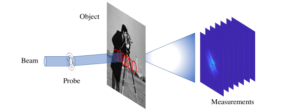
Ptychography is a popular imaging technique that combines both coherent diffractive imaging and scanning transmission microscopy. It is used in various industrial and scientific applications, including biology [49, 62, 79], crystallography [17], and optics [61, 66]. To perform a ptychographic experiment (see Figure 1), a coherent beam is scanned across the object of interest, where each scan may have overlapping positions with another. The scanning procedure provides a set of phaseless measurements that can be used to reconstruct an image of the object of interest.
Algorithms have been developed to solve the nonblind ptychography problem, where the probe is known, or more generally the phase retrieval problem. One of the most popular methods is the ptychographical iterative engine (PIE) [59], which applies gradient descent to the object using each measurement sequentially. Convergence analysis of PIE is provided in [50]. Other gradient-based methods for phase retrieval include Wirtinger flow [7] and its variants [15, 76, 78], which use adaptive step sizes and careful initialization based on spectral method. PIE is also one class of projection algorithms for phase retrieval, where the object update is projected onto a nonconvex modulus constraint set. Other projection-based algorithms are hybrid projection-reflection [1], Douglas-Rachford splitting [63], and the relaxed averaged alternating reflections [45]. For Douglas-Rachford splitting, fixed-point analysis and local, linear convergence were studied extensively [13, 14, 22]. The phase retrieval problem can be formulated as variational models [12, 71] that are solved by alternating direction method of multipliers (ADMM) [5] or proximal alternating linearized minimization [3]. Incorporating total variation regularization [10, 11, 12] improves the performance and robustness of these models, especially when the magnitude measurements are corrupted by noise.
Some algorithms for the nonblind ptychography problems were extended to jointly solve for the probe and object in the more challenging, blind ptychography problem, where the probe is unknown. Later refinements to PIE led to ePIE [47] and rPIE [46], which apply gradient descent updates with adaptive, stable step sizes to both the object and the probe. A convergence analysis of ePIE is provided in [51]. A Wirtinger flow algorithm was extended to blind polychromatic ptychography via alternating minimization and was proven to sublinearly converge to a stationary point [23]. A semi-implicit relaxed version of DR [56] was proposed as a robust algorithm to solve for both probe and object, especially with sparse data. Based on Kurdyka-Łojasiewicz assumptions [3], globally convergent algorithms, such as ADMM [8] and proximal alternating linearized minimization [27], were proposed for blind ptychography.
Large-scale ptychography, characterized by a substantial number of scans, presents challenges in terms of memory usage and computational cost for existing algorithms. Parallel algorithms have been developed to address these challenges. For example, an asynchronous, parallel version of ePIE was implemented on GPUs, where sub-images from partitioned measurement sets are fused together [52]. Additionally, a parallel version of relaxed averaged alternating reflections was adapted for GPU implementation [18]. However, these parallel algorithms often rely on GPUs, which may not be universally available. Alternatively, some algorithms designed for large-scale ptychography without high-performance computing resources have been proposed. For instance, a multigrid optimization framework accelerates gradient-based methods for phase retrieval [72], while an overlapping domain decomposition method combined with ADMM enables a highly parallel algorithm with good load balance [9]. A batch-based ADMM algorithm [74] was proposed to iteratively process a subset of measurement data instead of all for image reconstruction. Overall, these algorithms require careful tailoring specific to ptychography to demonstrate their benefits. Notably, to the best of our knowledge, a batch-based, stochastic ADMM algorithm for large-scale ptychography has yet to be developed. By incorporating stochastic gradient descent (SGD) [57], stochastic ADMM may be able to find better solutions [34] than the deterministic ADMM algorithms [8, 10, 11, 74] for the ptychography problem that is formulated as a nonconvex optimization problem. Moreover, being batch based, it would be computationally practical for practitioners without access to multiple cores for parallel computing.
To improve the image reconstruction quality in phase retrieval, total variation (TV) [60] has been incorporated for the cases when the measurements are corrupted with Gaussian noise [11] or with Poisson noise [10]. Both cases consider the isotropic TV approximation
| (1) |
where is an image, and are the horizontal and vertical difference operators, respectively, and and are the th entries in lexicographic ordering of and , respectively. However, it has been known that isotropic TV tends to blur oblique edges. An alternative approximation that preserves sharper edges is the anisotropic TV [19]:
| (2) |
Overall, TV is meant to approximate the “norm” of the image gradient, i.e., , because TV is based on the norm, a convex relaxation of . A nonconvex alternative to is , which performs well in recovering sparse solutions in various compressed sensing problems [41, 42, 43, 75]. The superior performance of in sparse recovery has motivated the development of the weighted difference of anisotropic and isotropic total variation (AITV) [44], which applies on each gradient vector of an image. Mathematically, AITV is formulated by
| (3) |
AITV has demonstrated better performance than TV in image denoising, image deconvolution, image segmentation, and MRI reconstruction [6, 44, 55], especially in preserving sharper edges.
In this work, we focus on addressing the large-scale ptychography problem with measurements corrupted by Gaussian or Poisson noise. To enhance image reconstruction quality, we incorporate AITV regularization within a general variational framework. The problem is then solved using an ADMM algorithm, where some subproblems are approximated by SGD [57]. However, direct application of SGD to the ptychography subproblem is not straightforward. Therefore, we demonstrate the appropriate adaptation of SGD to develop our specialized stochastic ADMM algorithm. Furthermore, we leverage the inherent structure embedded in the experiment such as per-pixel illumination strength and automate the selection of optimal step sizes within the minibatch regime. Unlike traditional methods using all measurements per iteration, our stochastic ADMM algorithm iteratively processes a random batch of measurements, resulting in accurate and efficient ptychographic reconstruction.
The paper is organized as follows. In Section 2, we describe the AITV-regularized variational models to solve the image ptychography problem. Within this section, we design the stochastic ADMM algorithms to solve these models. Convergence analysis of the stochastic ADMM algorithm follows in Section 3. In Section 4, we illustrate the performance of our proposed stochastic ADMM algorithms and compare them with other competing algorithms. Lastly, in Section 5, we conclude the paper with summary and future works.
2 Mathematical Model
We first describe basic notations used throughout the paper. Let be an vector that represents an image in lexicographical order, where the rows of an image matrix are transposed and stacked consecutively into one vector. The vector is a vector whose entries are all ones. Superscripts ⊤ and ∗ denote the real and conjugate transpose of a matrix, respectively. The sign of a complex value is given by
The sign of a vector is denoted by and is defined elementwise by The vector has 1 as the th component while all other entries are zeros. For , its th entry is . We define the following norms on :
The discrete gradient operator when specifically applied to the image is given by , where and are the forward horizontal and vertical difference operators. More specifically, the th entry of is defined by
| (4) |
where
and
We also define the proximal operator of a function as
Lastly, considering complex functions, we compute their gradient according to Wirtinger calculus [35].
We now describe the 2D ptychography in the discrete setting based on the notations in [8]. Let be the object of interest with pixels and be the localized 2D probe with pixels, where . Both the object and the probe are expressed as vectors in lexicographical order. We denote the set of masks by for total scanning positions, where each is a binary matrix that corresponds to the th scanning window of the probe on the object . As result, represents a different subwindow of the object . The set of phaseless measurements is obtained by , where is the normalized 2D discrete Fourier operator, is the elementwise multiplication, and is the elementwise absolute value of a vector. We note that the Fourier operator is unitary, i.e., and for any . For each , the measurement and the mask matrix form together the th scan information . Throughout the paper, we assume that for each , there exists such that . This assumption ensures that each pixel of an image is scanned at least once.
The blind ptychographic phase retrieval problem is expressed as follows:
| (5) |
When the probe is known, (5) reduces to the non-blind case where we only find . Suppose that the measurements are corrupted by independent and identically distributed (iid) noise. The blind variational model [8] is formulated by
| (6) |
where
| (7) |
Note that is elementwise square root. The AGM metric is suitable when the magnitude measurements , are corrupted by Gaussian noise, while the IPM metric is appropriate when the measurements are corrupted by Poisson noise. Nevertheless, AGM can also be used for the Poisson noise case because it is a variance-stablizing transform [48] and an approximation for IPM [64].
2.1 AITV model
To improve image recovery in blind ptychography, we propose a class of AITV-regularized variants of (6):
| (8) |
The non-smoothness of the objective function (8) with respect to and motivates the development of an ADMM algorithm for solving it. Specifically, we introduce auxiliary variables to represent , and to represent . These auxiliary variables play a crucial role in handling the non-smoothness of the objective function and enable the effective utilization of the ADMM framework for optimization. As a result, we obtain an equivalent constrained optimization problem
| (9) |
The augmented Lagrangian of (9) is
| (10) |
where denotes the real component of a complex number; denotes the complex inner product between two vectors; and are Lagrange multipliers; and are penalty parameters. The ADMM algorithm iterates as follows:
| (11a) | ||||
| (11b) | ||||
| (11c) | ||||
| (11d) | ||||
| (11e) | ||||
| (11f) | ||||
We explain how to solve each subproblem and adapt it in the stochastic, batch-based setting, where at each iteration we only have a randomly sampled mini-batch of scan information available such that . As a result, (11e) reduces to
| (11e′) |
2.1.1 -subproblem
Solving (11a) simplifies to solving independently, so we only need to update ’s whose corresponding scan information is available. Let be a diagonal matrix whose diagonal is . Then for each , we have
| (12) |
where since . Because the proximal operator for each fidelity term in (7) has a closed-form solution provided in [10, 11], the overall update is
| (13) |
2.1.2 -subproblem
The -subproblem (11b) can be rewritten as
| (14) |
Instead of using all scan information, we develop an alternative update scheme that uses only of them. Instead of solving (11b) exactly, we linearize it as done in [40, 54] to obtain
| (15) |
for some constant at iteration . Let so that we have
Then (15) is equivalent to performing gradient descent with step size :
| (16) |
Because we only have scan information available, we replace the update term in (16) with its stochastic estimate as:
| (17) |
For simplicity, we choose the SGD estimator [4, 57] as :
| (18) |
Similar to the PIE family algorithm [46, 47, 59], we further extend (18) by incorporating spatially varying illumination strength modeled as
| (19) |
where and division is elementwise. Incorporating into (18), we have another class of stochastic estimators
| (20) |
2.1.3 -subproblem
Expanding (11c) gives
| (21) |
which means that the solution can be solved elementwise. As a result, the subproblem simplifies to
| (22) |
A closed-form solution for the proximal operator of is provided in [41] but only for real-valued vectors. We generalize it to the complex case in Lemma 2.1, whose proof is delayed to Appendix A.
Lemma 2.1.
Given , , and , we have the following cases:
-
1.
When , we have
-
2.
When , we have as a 1-sparse vector such that one chooses an index and have
-
3.
When , we have .
Then is an optimal solution to
| (23) |
2.1.4 -subproblem
(11d) can be rewritten as
| (24) |
which implies that must satisfy the first-order optimality condition
| (25) |
where the Laplacian . Since the coefficient matrix of is invertible, solving (25) can be performed exactly, but it could be computationally expensive if the matrix system is extremely large because of the size of . Since the coefficient matrix tends to be sparse, conjugate gradient [28] can be used to solve (25) like in [10, 11], but it needs access to all scan information and requires at most iterations to attain an exact solution, assuming exact arithmetic. Moreover, it is sensitive to roundoff error [25].
Alternatively, we linearize (24) to obtain the gradient descent step with step size :
| (26) |
Approximating by its stochastic estimator that only has access to scans, we have the SGD step:
| (27) |
To design candidates for , we will use the following lemma:
Lemma 2.2.
Let . If for some index , then for any , we have .
Proof.
We have ∎
For brevity, we denote the vectors
| (28) |
At each pixel , (26) becomes
| (29) |
By Lemma 2.2, since , we have if , which means that pixel is not scanned by the mask matrix . For each , we define to be the set of indices corresponding to the mask matrices that scan pixel . As a result, (29) reduces to and can be rewritten as
| (30) |
Let be the set of indices corresponding to the mask matrices available at iteration that scan pixel . Since the SGD estimator [4, 57] of is , one candidate stochastic estimator (up to a constant multiple at each pixel) for is , where
| (31) |
for . Similar to the -subproblem, we further extend (31) to incorporate spatially varying illumination strength. Let
| (32) |
where . Then we have the following stochastic estimator as
| (33) |
for .
Input: set of scan information ; model parameters , ; penalty parameters ; sequence of step sizes ; batch size ; PIE factors .
Output: ,
3 Convergence Analysis
We discuss the convergence of Algorithm 1. Although global convergence for ADMM can be established using Kurdyka-Łojasiewicz assumptions [69], the result does not apply for our models because they contain the gradient operator, which does not satisfy the necessary surjectivity assumption. Hence, we will prove up to subsequential convergence. The convergence analysis is based on the analyses done in [10, 11, 71], where under certain assumptions, they showed that the iterate subsequences of the ADMM algorithms converge to Karush-Kuhn-Tucker (KKT) points. To simplify notation, let and . A KKT point of the Lagrangian (10) satisfies the KKT conditions given by
| (34a) | ||||
| (34b) | ||||
| (34c) | ||||
| (34d) | ||||
| (34e) | ||||
| (34f) | ||||
Let denote the expectation conditioned on the past sequence of iterates . More specifically, if is the sigma algebra generated by the mini-batches , then . We impose the following assumption:
Assumption 3.1.
Let be a sequence of iterates generated by Algorithm 1. For brevity, define and at each iteration .
Suppose that at each iteration , the stochastic gradient estimators
and satisfy the following:
-
(a)
Unbiased estimation:
(35) (36) -
(b)
Expected smoothness: there exist constants such that
(37) (38)
Remark 1.
Assumption 3.1(a)is standard in the analysis of many stochastic optimization algorithms [4, 36]. Assumption 3.1(b) was first proposed in [33] as a more general, weaker assumption on the second moment of the stochastic gradient than the other standard assumptions, such as bounded variance [36] and relaxed growth condition [4].
To prove the convergence of Algorithm 1, we require the following preliminary results. Under some conditions, Lemma 3.2 bounds the iterates generated by Algorithm 1 and the gradients . Moreover, it shows that the stochastic gradients have bounded variance. Lemma 3.3 provides useful inequalities while Proposition 3.4 establishes that the gradients subsequentially converge to zero. The convergence of Algorithm 1 is finally established in Theorem 3.5. All proofs are delayed to Appendix B.
Lemma 3.2.
Lemma 3.3.
Proposition 3.4.
Theorem 3.5.
Remark 2.
Similar to [10, 71], we impose the assumption that is bounded to assist with the convergence analysis. This assumption can be removed by imposing box constraints onto the primal variables as done in [8, 11, 27], but we leave it as a future direction to develop a globally convergent algorithm to solve (8) with these box constraints. We note that the requirement is rather strong, but similar assumption was made in other nonconvex ADMM algorithms [32, 39, 65, 73] that do not satisfy the necessary assumptions for global convergence [69]. Lastly, the step size condition (LABEL:eq:step_size_condition) is a standard assumption in proving convergence of stochastic algorithms [4, 57].
4 Numerical Results
In this section, we evaluate the performance of Algorithm 1 on two complex images presented in Figure LABEL:fig:test_image. The chip image (Figures LABEL:fig:chip_mag-LABEL:fig:chip_phase) has image size , while the cameraman/baboon image (Figures LABEL:fig:cameraman_mag-LABEL:fig:cameraman_phase) has image size . The probe size used for both images is , and the scanning patterns of the probes are shown in Figures LABEL:fig:chip_scan_pattern,LABEL:fig:cameraman_scan_pattern. In total, we have measurements per image. The measurements are either corrupted by Gaussian noise or Poisson noise as follows:
| (46) |
where is a multivariate Gaussian distribution with zero mean and covariance matrix and for some constant . Note that Poisson noise is stronger when is smaller.
For numerical evaluation, we compute the Structure Similarity Index Measure (SSIM) [70] between the reconstructed image and the ground-truth image for the magnitude and phase, separately, where is adjusted for scaling by and translation by and We compare the proposed stochastic ADMM algorithms with its deterministic, full-batch counterparts (i.e., (14) and (25) are solved exactly) and its isotropic TV (isoTV) counterparts based on [10, 11]. The results are also compared with Douglas-Rachford splitting [8, 63], rPIE [47], and PHeBIE [27].
We initialize when using AGM for Gaussian-corrupted measurements and when using IPM for Poisson-corrupted measurements. When performing the blind experiments using Algorithm 1, is initialized as the perturbation of the ground-truth probe. The magnitude differences between the initial and ground-truth probes are shown in Figures LABEL:fig:chip_diff_probe,LABEL:fig:cameraman_diff_probe. The selected parameters, except for , are summarized in Table LABEL:tab:alg_param. The initial step sizes for and are determined empirically, and motivated by (LABEL:eq:step_size_condition), we decrease them by a factor of 10 at the and of the total epochs. Decreasing the step size in this way is a popular technique, especially in the deep learning community [24, 26]. Inspired from [24], the step sizes are multiplied by a factor of so that they scale by the batch size. For AITV regularization, we examine and determine that yields the best results across all of our numerical examples. The batch sizes we examine are for Gaussian noise and for Poisson noise. For each parameter setting and image, we run three trials to obtain the mean SSIM values.
All experiments are performed in MATLAB R2022b on a Dell laptop with a 1.80 GHz Intel Core i7-8565U processor and 16.0 GB RAM. The code for the experiments is available at https://github.com/kbui1993/Stochastic_ADMM_Ptycho.
4.1 Gaussian noise
The SNR of the noisy measurements [10] is given by
so determined by the SNR, the noise level in (46) is calculated by
For both the non-blind and blind cases, we examine the case when the noisy measurements have , so we set the regularization parameter . Table LABEL:tab:gaussian_result records the SSIMs of the magnitude and phase components of the test images for the non-blind and blind cases. For all cases, DR, rPIE, and PHeBIE yield the worst magnitude SSIMs, and AITV attains better magnitude and phase SSIMs than its corresponding isoTV counterpart. The stochastic AITV () has slightly lower magnitude SSIMs by at most than the best results obtained from the deterministic, full-batch AITV. In fact, stochastic AITV attains the second best magnitude SSIMs in three out of the four cases considered. On the other hand, stochastic AITV () has the best phase SSIMs, such as outperforming their deterministic counterparts by up to 0.19 for the the blind case of the cameraman/baboon image. In general, the stochastic algorithm does best in recovering the phase components while recovering the magnitude components with comparable quality as the deterministic algorithm.
The reconstructed images for the non-blind experiments are presented in Figure LABEL:fig:agm_nonblind. DR, rPIE, PHeBIE, and the stochastic algorithms have artifacts in all four corners of the magnitude images because the corners are scanned significantly less than in the middle of the image. However, the deterministic AITV has no artifacts because (25) is solved exactly for the image solution . As a result, it has higher magnitude SSIMs than their stochastic counterparts. Nevertheless, the stochastic algorithms yield better phase images with less noise artifacts than any other algorithms. For example, the phase images of Figure LABEL:fig:cameraman_phase reconstructed from stochastic isoTV and AITV have the least amount of artifacts from the cameraman in the magnitude component.
Figure LABEL:fig:blind_agm shows the results of the blind algorithms. The phase images reconstructed by the deterministic AITV, DR, rPIE and PHeBIE are significantly worse than the stochastic algorithms. For example in Figure LABEL:fig:chip_phase, the contrasts of the reconstructed images by the deterministic AITV, DR, and PHeBIE are inconsistent as they become darker from left to right while the contrasts are more consistent with the stochastic algorithms. For Figure LABEL:fig:cameraman_phase, the stochastic algorithms perform the best in recovering the phase image while deterministic AITV is unable to recover the left half of the image and DR, rPIE, and PHeBIE have strong remnants of the cameraman present. Like in the non-blind case, stochastic AITV reconstructs the phase image the best. Overall, recovering the phase component in the blind case is more difficult than the nonblind case because of the artifacts created by the inherent ambiguities encountered when recovering both the probe and the object [2, 20, 21].
In Figure LABEL:fig:agm_convergence, we examine the convergence of the blind algorithms applied to the cameraman/baboon image by recording their AGM values for each epoch. We omit the convergence curves of isoTV since they are similar to their AITV counterparts. Overall, the curves for our proposed stochastic algorithms are decreasing, validating the numerical convergence of Algorithm 1 with AGM fidelity. However, their curves are slightly above the deterministic ADMM algorithm and rPIE. The reason why rPIE outperforms the AITV algorithms is because it seeks to only minimize AGM while the AITV algorithms minimize a larger objective function given by (10). Overall, after several hundred epochs, our proposed stochastic algorithms can give comparable AGM values as the deterministic AITV and rPIE algorithms.
Figure LABEL:fig:agm_compute shows the magnitude/phase SSIMs of the cameraman/baboon image with respect to computational time in seconds when running each blind algorithm for 600 epochs. Although DR, rPIE, and PHeBIE finish running 600 epochs faster than the AITV algorithms, the stochastic AITV algorithms can attain magnitude SSIM higher than 0.90 and phase SSIM higher than 0.70 in about 500 seconds, thereby outperforming DR, rPIE, and PHeBIE in faster time. Moreover, because the stochastic AITV algorithms solve (14) and (25) inexactly by SGD, they finish running 600 epoches faster than the deterministic AITV by at least 2000 seconds or 33.33 minutes. Apparently, larger batch size allows the stochastic algorithm to finish faster.
We examine the effect of the AITV regularization parameter in (8) on the image reconstruction quality. The value of is adjusted depending on the amount of noise corrupting the measurements. If is chosen to be small, AITV regularization will have a minimal impact on the image reconstruction, resulting in a potentially noisy image. However, if is chosen to be large, AITV will oversmooth the reconstructed image. Therefore, a moderate value of is recommended. For the AITV algorithms, we test for the blind case on the complex image given by Figures LABEL:fig:cameraman_mag-LABEL:fig:cameraman_phase, whose measurements are corrupted by Gaussian noise of SNR = 40. According to Figure LABEL:fig:agm_lambda, the magnitude/phase SSIMs have a concave relationship with the AITV regularization parameter , where the SSIMs appear to peak at for most AITV algorithms.
Lastly, we analyze the robustness of the blind algorithms applied to the cameraman/baboon image whose measurements are corrupted by different levels of Gaussian noise, from SNR 25 to 65. The regularization parameter is adjusted for different noise level of the measurements: for SNR = 25; for SNR = 30, 35; for SNR =40, 45; for SNR = 50, 55, 60; and for SNR = 65. The algorithms ran for 600 epochs and the magnitude and phase SSIMs across different SNRs are plotted in Figure LABEL:fig:robust_agm. For , the deterministic isoTV and AITV algorithms have the best magnitude SSIMs than the other algorithms while their stochastic counterparts have slightly lower SSIMs. When , the stochastic algorithms perform the best. In fact, stochastic AITV has magnitude SSIM at least 0.90 across all noise levels considered. For the phase image, the stochastic algorithms have the highest SSIMs up to SNR = 55. For , the rPIE algorithm has the best phase SSIM while stochastic AITV has the second best. Overall, stochastic AITV is the most stable across different levels of Gaussian noise.
4.2 Poisson noise
| Non-blind | Blind | |||||||
| Chip | Cameraman/Baboon | Chip | Cameraman/Baboon | |||||
| mag. SSIM | phase SSIM | mag. SSIM | phase SSIM | mag. SSIM | phase SSIM | mag. SSIM | phase SSIM | |
| DR | 0.8523 | 0.8455 | 0.8704 | 0.5043 | 0.8431 | 0.7387 | 0.7630 | 0.2529 |
| rPIE | 0.0206 | 0.1400 | 0.0701 | 0.2136 | 0.0213 | 0.1416 | 0.0700 | 0.2137 |
| PHeBIE | 0.9404 | 0.9398 | 0.9271 | 0.6791 | 0.9280 | 0.9082 | 0.8678 | 0.5470 |
| isoTV | 0.9491 | 0.9130 | 0.9364 | 0.7063 | 0.9402 | 0.8964 | 0.9256 | 0.7075 |
| isoTV | 0.9411 | 0.9164 | 0.9338 | 0.6892 | 0.9343 | 0.9029 | 0.9221 | 0.6911 |
| isoTV | 0.9377 | 0.9319 | 0.9321 | 0.6788 | 0.9339 | 0.9236 | 0.9186 | 0.6810 |
| isoTV | 0.9379 | 0.9382 | 0.9313 | 0.6768 | 0.9355 | 0.9306 | 0.9175 | 0.6788 |
| isoTV (full batch) | 0.9767 | 0.9590 | 0.9773 | 0.7093 | 0.9655 | 0.9192 | 0.9588 | 0.4920 |
| AITV | 0.9594 | 0.9598 | 0.9384 | 0.7237 | 0.9484 | 0.9551 | 0.9298 | 0.7384 |
| AITV | 0.9655 | 0.9634 | 0.9447 | 0.7168 | 0.9551 | 0.9548 | 0.9381 | 0.7303 |
| AITV | 0.9645 | 0.9641 | 0.9473 | 0.7012 | 0.9559 | 0.9543 | 0.9373 | 0.7082 |
| AITV | 0.9629 | 0.9634 | 0.9462 | 0.6957 | 0.9549 | 0.9535 | 0.9347 | 0.7012 |
| AITV (full batch) | 0.9803 | 0.9644 | 0.9782 | 0.7084 | 0.9741 | 0.9354 | 0.9671 | 0.4975 |
.
For both the non-blind and blind case, we examine the measurements corrupted with Poisson noise with (SNR for Figures LABEL:fig:chip_mag-LABEL:fig:chip_phase; SNR for Figures LABEL:fig:cameraman_mag-LABEL:fig:cameraman_phase) according to (46). We set the regularization parameter . The numerical results are recorded in Table 1.
Across all cases, deterministic AITV attains the highest magnitude SSIMs and stochastic AITV attains the highest phase SSIMs while rPIE performs the worst in reconstructing images from Poisson-corrupted measurements. Using AITV over isoTV, we observe improvement in both magnitude and phase SSIMs. Although the stochastic algorithms have lower magnitude SSIMs than their deterministic counterparts, the difference is at most 0.04 for AITV and at most 0.05 for isoTV. Moreover, the magnitude SSIMs from the stochastic algorithms remain above 0.91. Similar to the Gaussian noise case, stochastic AITV reconstructs the phase image well while recovering the magnitude image with satisfactory quality.
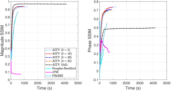
Figure 2 shows the magnitude/phase SSIMs of the cameraman/baboon image with respect to computational time in seconds when running each blind algorithm for 300 epochs. Like for the Gaussian case, the stochastic AITV algorithms can recover faster the complex image with better quality in both the magnitude and phase components than DR, rPIE, and PHeBIE. Moreover, the stochastic AITV algorithms finish running 300 epochs significantly faster than the deterministic AITV algorithm. In fact, with stochastic AITV, one can recover within 1000 seconds the complex image with magnitude SSIM higher than 0.90 and phase SSIM higher than 0.70. Overall, the stochastic algorithms are computationally efficient in recovering complex images with satisfactory quality.
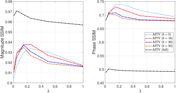
We perform sensitivity analysis of the AITV regularization parameter on the magnitude/phase SSIMs, where we test . The AITV algorithms ran for 300 epochs in the blind case on the complex image given by Figures LABEL:fig:cameraman_mag-LABEL:fig:cameraman_phase. The measurements are corrupted by Poisson noise with (SNR ). Figure 3 shows the impact of the AITV regularization parameter on the magnitude/phase SSIMs. Like for the AGM case, the SSIMs are concave with respect to , where they peak at .
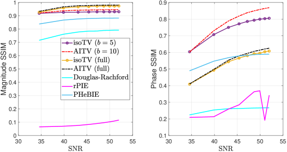
We examine the robustness of the blind algorithms on Figures LABEL:fig:cameraman_mag-LABEL:fig:cameraman_phase with different level of Poisson noise. The noise levels we examine are (SNR , respectively). We set the regularization parameter to be . The magnitude and phase SSIMs across different Poisson noise levels are plotted in Figure 4. We observe that the deterministic algorithms yield the best magnitude SSIMs while the stochastic algorithms yield the best phase SSIMs. Both DR and rPIE yield the worst results for both magnitude and phase components. Although stochastic AITV yields the third best SSIMs for the magnitude image, its SSIMs are at least 0.90. Moreover, it has the best phase SSIMs, significantly more than its deterministic counterpart by about 0.20. In summary, stochastic AITV is a robust method across different levels of Poisson noise.
5 Conclusion
In this study, we present a novel approach for image ptychography utilizing AITV-regularized variational models. These models effectively handle measurements corrupted by Gaussian or Poisson noise. To address the challenges posed by a large number of measurements, we develop a stochastic ADMM algorithm with adaptive step sizes inspired by the inherent structure of ptychography (e.g., per-pixel illumination strength). Our proposed method demonstrates the ability to reconstruct high-quality images from severely corrupted measurements, with particular emphasis on accurately recovering the phase component. Theoretical convergence of the stochastic ADMM algorithm is established under certain conditions, and our numerical experiments confirm both convergence and computational efficiency.
For future research, we aim to design a globally convergent algorithm for the AITV-regularized ptychography model with box constraints and provide convergence analysis with weaker assumptions than in Theorem 3.5. Additionally, we plan to explore the incorporation of variance-reduced stochastic gradient estimators such as SVRG [31] and SARAH [53]. These techniques have the potential to further enhance computational efficiency and improve the quality of image reconstruction. Lastly, we plan to develop a library of ptychography models regularized with other nonconvex variants of total variation, such as TV regularization [29, 37], log total variation [77], on the gradient [67, 68] and transformed total variation [30].
Acknowledgments
This material is based upon work supported by the U.S. Department of Energy, Office of Science, under contract number DE-AC02-06CH11357. We thank the two reviewers for their valuable feedback in improving the manuscript.
A Proof of Lemma 2.1
Proof.
If , then it is trivial, so for the rest of the proof, we assume that .
Suppose is the optimal solution to (23). Because is rotation invariant, we only need to examine and expand the quadratic term in (23). We see that
where is the angle between the components and . This term is minimized when for all . This means that for all such that , or otherwise would not be an optimal solution to (23). When or , we choose such that . Overall, we have .
Since , we can simplify (23) to an optimization problem with respect to given by
Next, we show that nonnegativity constraint is redundant, i.e.,
| (47) |
Let be the optimal solution to the right-hand optimization problem in (47) and . Comparing the optimal values between and , we have
which reduces to
| (48) |
However, if , then (48) is invalid because the left-hand side is negative. As a result, , implying that for all , so the nonnegativity constraint of the right-hand optimization problem in (47) is redundant. This follows that we have
Hence, by applying [41, Lemma 1] to the optimization problem, we establish the following:
-
(1)
When ,
-
(2)
When , is an optimal solution if and only if it satisfies if , and .
-
(3)
When , is an optimal solution if and only if it is a 1-sparse vector satisfying if , and .
-
(4)
When , .
When , we show that for a selected index we have
as an optimal solution. By construction, is a 1-sparse vector satisfying when . Since , we have
By satisfying the conditions in (2) and (3) above, is an optimal solution. Lastly, by multiplying by , we obtain the desired results. ∎
B Proofs of Section 3
Before proving our main results, we present preliminary tools necessary for the convergence analysis.
Definition B.1 ([38, 58]).
Let be a proper and lower semicontinuouous function and .
-
(a)
The Fréchet subdifferential of at the point is the set
-
(b)
The limiting subdifferential of at the point is the set
We note that the limiting subdifferential is closed [58]:
Lemma B.2 ([16], pg.129, Exercise 7).
Let be a sequence of random variables. If , then converges absolutely a.s.
Lemma B.3.
Let be an index set chosen uniformly at random from all subsets of with cardinality at iteration . For any , we have for infinitely many a.s.
Proof.
Since sampling from for each is independent and , we apply Second Borel-Cantelli Lemma to obtain the desired result. ∎
B.1 Proof of Lemma 3.2
Proof.
Because , we have and . From (11f), we have
| (49) |
so is bounded since is bounded. Because , it follows that is bounded. Combining the first case of (11e′) with the second case of (13), we have
| (50) |
If , then we have
If , we have two cases. For one case, if we have for all , then by (50), we have . For the other case, there exists . Then by (50), we have
Altogether, is bounded because is bounded. By (13), when is AGM, if , we have
or equivalently,
| (51) |
Similarly, when is IPM, we have the same inequality as (51). If , then as before, we have two cases. For the first case, if for all , then by (11e′), we have . Otherwise, there exists , so
Hence, we conclude that is bounded. Finally, we show that is bounded by examining (22). For each , we have two cases. For the first case, if there exists some such that
then by reverse triangle inequality, we have
Let
For the other case, if there exists such that
then by Lemma 2.1(i) and reverse triangle inequality, we have
which follows that
Altogether, we have
so is bounded because is bounded. Therefore, we establish that is bounded.
B.2 Proof of Lemma 3.3
Proof.
If is bounded, then there exists a constant such that for all . We establish that has a Lipschitz continuous gradient with respect to . At each iteration , we have
so for any , we estimate
Hence, we observe that has a Lipschitz continuous gradient with Lipschitz constant . By the descent property [8, Definition 1], at iteration we have
where the last equality is due to (17). Because we assume that is bounded and , (39)-(40) hold by Lemma 3.2. Taking the expectation conditioned on the iterations and , we obtain
The last inequality is due to Assumption 3.1(a) and (39). Taking total expectation gives us (41).
Similarly, we can estimate (42) because we can compute that has a Lipschitz continuous gradient with Lipschitz constant and follow the same steps as above by taking expectation conditioned on the first iterations and . ∎
B.3 Proof of Proposition 3.4
Proof.
By Lemma 3.2, is bounded. We see that
Because is bounded below according to (7) and is bounded, is bounded below by some constant . At iteration , we denote the following for the sake of brevity:
By (LABEL:eq:u_min), we have
for each , and by (13), we have
for each . Summing over all and adding the term to both sides of the inequality, we obtain . By (11c), we have , so taking expectation, we obtain
| (52) | ||||
| (53) |
In addition, we have
due to (11e′). Taking expectation gives
| (54) |
Similarly, we obtain
| (55) |
Summing up (41)-(42), (52)-(55), we have
| (56) |
Summing up , we obtain
where . Note that since serves as initialization. By (LABEL:eq:step_size_condition), we have and for all , which follows that . Rearranging the inequality and letting give us
By the summability assumption, the right-hand side is bounded. As a result, there exists a positive constant such that
By (LABEL:eq:step_size_condition), we have
which implies that for any ,
For any , we have
As , we obtain for any . Therefore, taking the limit as , we obtain
(45) is proven similarly by following the same steps. ∎
B.4 Proof of Theorem 3.5
Proof.
By Lemma 3.2, and are bounded and (39)-(40) hold. So, there exists such that for all . Recall that the SGD steps for are
Applying total expectation, summing over all , and using (LABEL:eq:step_size_condition) establish
| (57) | |||
| (58) |
By Lemma B.2, we have
| (59) | ||||
| (60) |
For the sake of brevity, we will omit “a.s.” in the rest of the proof. Earlier, in the proof of Lemma 3.2, we obtained
| (61) |
By (44)-(45) in Proposition 3.4, there exists a subsequence such that
| (62) | ||||
| (63) |
Because is bounded, there exists a subsequence such that . In addition, (59)-(63) hold for this subsequence.
Now we show that is a KKT point. From (61), we have
| (64) |
Since by the assumption, it follows that . For each , there exists for such that implies the following:
| (65) | ||||
| (66) | ||||
| (67) |
Note that (65) is due to ; (66) is due to ; and (67) is due to . Then, by Lemma B.3, there exists such that , so we have
after applying (50) and (65)-(67). Because is chosen arbitrarily, it follows that
| (68) |
Before proving the rest of the conditions, we need to show that and for each . By (60), (61), and (64), we have
| (69) |
Since is bounded, then for all for some constant . For , there exists such that implies the following:
| (70) | ||||
| (71) | ||||
| (72) |
Note that (70)-(71) are due to (59)-(60) and (72) is due to . By definition of , we have for all . For each , when , we establish that if , then
| (73) |
by (50) and (65), and if , then
by (50), (67), (68), and (70)-(72). Because is chosen arbitrarily, we have
| (74) |
Next we prove (34c). At iteration for each , the first-order optimality condition of (11a) is
For the IPM case, because for any , it follows that for all , so we do need to worry about for any iteration . By (68) and (74), we see that
and
By closedness of subdifferential, we establish that
References
References
- [1] H. H. Bauschke, P. L. Combettes, and D. R. Luke, Hybrid projection–reflection method for phase retrieval, Journal of the Optical Society of America A, 20 (2003), pp. 1025–1034.
- [2] T. Bendory, D. Edidin, and Y. C. Eldar, Blind phaseless short-time fourier transform recovery, IEEE Transactions on Information Theory, 66 (2019), pp. 3232–3241.
- [3] J. Bolte, S. Sabach, and M. Teboulle, Proximal alternating linearized minimization for nonconvex and nonsmooth problems, Mathematical Programming, 146 (2014), pp. 459–494.
- [4] L. Bottou, F. E. Curtis, and J. Nocedal, Optimization methods for large-scale machine learning, SIAM Review, 60 (2018), pp. 223–311.
- [5] S. Boyd, N. Parikh, and E. Chu, Distributed optimization and statistical learning via the alternating direction method of multipliers, Now Publishers Inc, 2011.
- [6] K. Bui, F. Park, Y. Lou, and J. Xin, A weighted difference of anisotropic and isotropic total variation for relaxed Mumford–Shah color and multiphase image segmentation, SIAM Journal on Imaging Sciences, 14 (2021), pp. 1078–1113.
- [7] E. J. Candes, X. Li, and M. Soltanolkotabi, Phase retrieval via Wirtinger flow: Theory and algorithms, IEEE Transactions on Information Theory, 61 (2015), pp. 1985–2007.
- [8] H. Chang, P. Enfedaque, and S. Marchesini, Blind ptychographic phase retrieval via convergent alternating direction method of multipliers, SIAM Journal on Imaging Sciences, 12 (2019), pp. 153–185.
- [9] H. Chang, R. Glowinski, S. Marchesini, X.-C. Tai, Y. Wang, and T. Zeng, Overlapping domain decomposition methods for ptychographic imaging, SIAM Journal on Scientific Computing, 43 (2021), pp. B570–B597.
- [10] H. Chang, Y. Lou, Y. Duan, and S. Marchesini, Total variation–based phase retrieval for Poisson noise removal, SIAM Journal on Imaging Sciences, 11 (2018), pp. 24–55.
- [11] H. Chang, Y. Lou, M. K. Ng, and T. Zeng, Phase retrieval from incomplete magnitude information via total variation regularization, SIAM Journal on Scientific Computing, 38 (2016), pp. A3672–A3695.
- [12] H. Chang, S. Marchesini, Y. Lou, and T. Zeng, Variational phase retrieval with globally convergent preconditioned proximal algorithm, SIAM Journal on Imaging Sciences, 11 (2018), pp. 56–93.
- [13] P. Chen and A. Fannjiang, Coded aperture ptychography: uniqueness and reconstruction, Inverse Problems, 34 (2018), p. 025003.
- [14] , Fourier phase retrieval with a single mask by douglas–rachford algorithms, Applied and computational harmonic analysis, 44 (2018), pp. 665–699.
- [15] Y. Chen and E. J. Candès, Solving random quadratic systems of equations is nearly as easy as solving linear systems, Communications on Pure and Applied Mathematics, 70 (2017), pp. 822–883.
- [16] K. L. Chung, A course in probability theory, Academic Press, 2001.
- [17] L. De Caro, D. Altamura, M. Arciniegas, D. Siliqi, M. R. Kim, T. Sibillano, L. Manna, and C. Giannini, Ptychographic imaging of branched colloidal nanocrystals embedded in free-standing thick polystyrene films, Scientific Reports, 6 (2016), pp. 1–8.
- [18] P. Enfedaque, H. Chang, B. Enders, D. Shapiro, and S. Marchesini, High performance partial coherent X-ray ptychography, in International Conference on Computational Science, Springer, 2019, pp. 46–59.
- [19] S. Esedoḡlu and S. J. Osher, Decomposition of images by the anisotropic Rudin-Osher-Fatemi model, Communications on Pure and Applied Mathematics, 57 (2004), pp. 1609–1626.
- [20] A. Fannjiang, Raster grid pathology and the cure, Multiscale Modeling & Simulation, 17 (2019), pp. 973–995.
- [21] A. Fannjiang and P. Chen, Blind ptychography: uniqueness and ambiguities, Inverse Problems, 36 (2020), p. 045005.
- [22] A. Fannjiang and Z. Zhang, Fixed point analysis of douglas–rachford splitting for ptychography and phase retrieval, SIAM Journal on Imaging Sciences, 13 (2020), pp. 609–650.
- [23] F. Filbir and O. Melnyk, Image recovery for blind polychromatic ptychography, SIAM Journal on Imaging Sciences, 16 (2023), pp. 1308–1337.
- [24] P. Goyal, P. Dollár, R. Girshick, P. Noordhuis, L. Wesolowski, A. Kyrola, A. Tulloch, Y. Jia, and K. He, Accurate, large minibatch SGD: Training Imagenet in 1 hour, arXiv preprint arXiv:1706.02677, (2017).
- [25] A. Greenbaum, Behavior of slightly perturbed Lanczos and conjugate-gradient recurrences, Linear Algebra and its Applications, 113 (1989), pp. 7–63.
- [26] K. He, X. Zhang, S. Ren, and J. Sun, Deep residual learning for image recognition, in Proceedings of the IEEE Conference on Computer Vision and Pattern Recognition, 2016, pp. 770–778.
- [27] R. Hesse, D. R. Luke, S. Sabach, and M. K. Tam, Proximal heterogeneous block implicit-explicit method and application to blind ptychographic diffraction imaging, SIAM Journal on Imaging Sciences, 8 (2015), pp. 426–457.
- [28] M. R. Hestenes and E. Stiefel, Methods of conjugate gradients for solving linear systems, Journal of Research of the National Bureau of Standards, 49 (1952), p. 409.
- [29] M. Hintermüller and T. Wu, Nonconvex TVq-models in image restoration: Analysis and a trust-region regularization–based superlinearly convergent solver, SIAM Journal on Imaging Sciences, 6 (2013), pp. 1385–1415.
- [30] L. Huo, W. Chen, H. Ge, and M. K. Ng, Stable image reconstruction using transformed total variation minimization, SIAM Journal on Imaging Sciences, 15 (2022), pp. 1104–1139.
- [31] R. Johnson and T. Zhang, Accelerating stochastic gradient descent using predictive variance reduction, Advances in Neural Information Processing Systems, 26 (2013), pp. 315–323.
- [32] Y.-F. Ke and C.-F. Ma, Alternating direction methods for solving a class of Sylvester-like matrix equations, Linear and Multilinear Algebra, 65 (2017), pp. 2268–2292.
- [33] A. Khaled and P. Richtárik, Better theory for SGD in the nonconvex world, Transactions on Machine Learning Research, (2023).
- [34] B. Kleinberg, Y. Li, and Y. Yuan, An alternative view: When does SGD escape local minima?, in International conference on machine learning, PMLR, 2018, pp. 2698–2707.
- [35] K. Kreutz-Delgado, The complex gradient operator and the CR-calculus, arXiv preprint arXiv:0906.4835, (2009).
- [36] G. Lan, First-order and stochastic optimization methods for machine learning, vol. 1, Springer, 2020.
- [37] A. Lanza, S. Morigi, and F. Sgallari, Constrained tv model for image restoration, Journal of Scientific Computing, 68 (2016), pp. 64–91.
- [38] J. Li, Solving blind ptychography effectively via linearized alternating direction method of multipliers, Journal of Scientific Computing, 94 (2023), p. 19.
- [39] H. Liu, K. Deng, H. Liu, and Z. Wen, An entropy-regularized ADMM for binary quadratic programming, Journal of Global Optimization, (2022), pp. 1–33.
- [40] Q. Liu, X. Shen, and Y. Gu, Linearized ADMM for nonconvex nonsmooth optimization with convergence analysis, IEEE Access, 7 (2019), pp. 76131–76144.
- [41] Y. Lou and M. Yan, Fast L1–L2 minimization via a proximal operator, Journal of Scientific Computing, 74 (2018), pp. 767–785.
- [42] Y. Lou, P. Yin, Q. He, and J. Xin, Computing sparse representation in a highly coherent dictionary based on difference of and , Journal of Scientific Computing, 64 (2015), pp. 178–196.
- [43] Y. Lou, P. Yin, and J. Xin, Point source super-resolution via non-convex based methods, Journal of Scientific Computing, 68 (2016), pp. 1082–1100.
- [44] Y. Lou, T. Zeng, S. Osher, and J. Xin, A weighted difference of anisotropic and isotropic total variation model for image processing, SIAM Journal on Imaging Sciences, 8 (2015), pp. 1798–1823.
- [45] D. R. Luke, Relaxed averaged alternating reflections for diffraction imaging, Inverse Problems, 21 (2004), p. 37.
- [46] A. Maiden, D. Johnson, and P. Li, Further improvements to the ptychographical iterative engine, Optica, 4 (2017), pp. 736–745.
- [47] A. M. Maiden and J. M. Rodenburg, An improved ptychographical phase retrieval algorithm for diffractive imaging, Ultramicroscopy, 109 (2009), pp. 1256–1262.
- [48] S. Marchesini, H. Krishnan, B. J. Daurer, D. A. Shapiro, T. Perciano, J. A. Sethian, and F. R. Maia, Sharp: a distributed gpu-based ptychographic solver, Journal of applied crystallography, 49 (2016), pp. 1245–1252.
- [49] J. Marrison, L. Räty, P. Marriott, and P. O’Toole, Ptychography–a label free, high-contrast imaging technique for live cells using quantitative phase information, Scientific Reports, 3 (2013), pp. 1–7.
- [50] O. Melnyk, Stochastic amplitude flow for phase retrieval, its convergence and doppelgängers, arXiv preprint arXiv:2212.04916, (2022).
- [51] , Convergence properties of gradient methods for blind ptychography, arXiv preprint arXiv:2306.08750, (2023).
- [52] Y. S. Nashed, D. J. Vine, T. Peterka, J. Deng, R. Ross, and C. Jacobsen, Parallel ptychographic reconstruction, Optics Express, 22 (2014), pp. 32082–32097.
- [53] L. M. Nguyen, J. Liu, K. Scheinberg, and M. Takáč, SARAH: A novel method for machine learning problems using stochastic recursive gradient, in International Conference on Machine Learning, PMLR, 2017, pp. 2613–2621.
- [54] Y. Ouyang, Y. Chen, G. Lan, and E. Pasiliao Jr, An accelerated linearized alternating direction method of multipliers, SIAM Journal on Imaging Sciences, 8 (2015), pp. 644–681.
- [55] F. Park, Y. Lou, and J. Xin, A weighted difference of anisotropic and isotropic total variation for relaxed mumford-shah image segmentation, in 2016 IEEE International Conference on Image Processing (ICIP), IEEE, 2016, pp. 4314–4318.
- [56] M. Pham, A. Rana, J. Miao, and S. Osher, Semi-implicit relaxed Douglas-Rachford algorithm (sDR) for ptychography, Optics Express, 27 (2019), pp. 31246–31260.
- [57] H. Robbins and S. Monro, A stochastic approximation method, The Annals of Mathematical Statistics, (1951), pp. 400–407.
- [58] R. T. Rockafellar and R. J.-B. Wets, Variational analysis, vol. 317, Springer Science & Business Media, 2009.
- [59] J. M. Rodenburg and H. M. Faulkner, A phase retrieval algorithm for shifting illumination, Applied Physics Letters, 85 (2004), pp. 4795–4797.
- [60] L. I. Rudin, S. Osher, and E. Fatemi, Nonlinear total variation based noise removal algorithms, Physica D: nonlinear phenomena, 60 (1992), pp. 259–268.
- [61] Y. Shechtman, Y. C. Eldar, O. Cohen, H. N. Chapman, J. Miao, and M. Segev, Phase retrieval with application to optical imaging: a contemporary overview, IEEE Signal Processing Magazine, 32 (2015), pp. 87–109.
- [62] A. Suzuki, K. Shimomura, M. Hirose, N. Burdet, and Y. Takahashi, Dark-field X-ray ptychography: Towards high-resolution imaging of thick and unstained biological specimens, Scientific Reports, 6 (2016), pp. 1–9.
- [63] P. Thibault, M. Dierolf, O. Bunk, A. Menzel, and F. Pfeiffer, Probe retrieval in ptychographic coherent diffractive imaging, Ultramicroscopy, 109 (2009), pp. 338–343.
- [64] P. Thibault and M. Guizar-Sicairos, Maximum-likelihood refinement for coherent diffractive imaging, New Journal of Physics, 14 (2012), p. 063004.
- [65] Z. Tu, J. Lu, H. Zhu, H. Pan, W. Hu, Q. Jiang, and Z. Lu, A new nonconvex low-rank tensor approximation method with applications to hyperspectral images denoising, Inverse Problems, 39 (2023), p. 065003.
- [66] A. Walther, The question of phase retrieval in optics, Optica Acta: International Journal of Optics, 10 (1963), pp. 41–49.
- [67] C. Wang, M. Tao, C.-N. Chuah, J. Nagy, and Y. Lou, Minimizing l 1 over l 2 norms on the gradient, Inverse Problems, 38 (2022), p. 065011.
- [68] C. Wang, M. Tao, J. G. Nagy, and Y. Lou, Limited-angle ct reconstruction via the l_1/l_2 minimization, SIAM Journal on Imaging Sciences, 14 (2021), pp. 749–777.
- [69] Y. Wang, W. Yin, and J. Zeng, Global convergence of ADMM in nonconvex nonsmooth optimization, Journal of Scientific Computing, 78 (2019), pp. 29–63.
- [70] Z. Wang, A. C. Bovik, H. R. Sheikh, and E. P. Simoncelli, Image quality assessment: from error visibility to structural similarity, IEEE Transactions on Image Processing, 13 (2004), pp. 600–612.
- [71] Z. Wen, C. Yang, X. Liu, and S. Marchesini, Alternating direction methods for classical and ptychographic phase retrieval, Inverse Problems, 28 (2012), p. 115010.
- [72] S. Wu Fung and Z. Di, Multigrid optimization for large-scale ptychographic phase retrieval, SIAM Journal on Imaging Sciences, 13 (2020), pp. 214–233.
- [73] Y. Xu, W. Yin, Z. Wen, and Y. Zhang, An alternating direction algorithm for matrix completion with nonnegative factors, Frontiers of Mathematics in China, 7 (2012), pp. 365–384.
- [74] L. Yang, Z. Liu, G. Zheng, and H. Chang, Batch-based alternating direction methods of multipliers for Fourier ptychography, Optics Express, 30 (2022), pp. 34750–34764.
- [75] P. Yin, Y. Lou, Q. He, and J. Xin, Minimization of for compressed sensing, SIAM Journal on Scientific Computing, 37 (2015), pp. A536–A563.
- [76] Z. Yuan, H. Wang, and Q. Wang, Phase retrieval via sparse Wirtinger flow, Journal of Computational and Applied Mathematics, 355 (2019), pp. 162–173.
- [77] B. Zhang, G. Zhu, and Z. Zhu, A TV-log nonconvex approach for image deblurring with impulsive noise, Signal Processing, 174 (2020), p. 107631.
- [78] H. Zhang, Y. Zhou, Y. Liang, and Y. Chi, A nonconvex approach for phase retrieval: Reshaped Wirtinger flow and incremental algorithms, Journal of Machine Learning Research, 18 (2017).
- [79] L. Zhou, J. Song, J. S. Kim, X. Pei, C. Huang, M. Boyce, L. Mendonça, D. Clare, A. Siebert, C. S. Allen, et al., Low-dose phase retrieval of biological specimens using cryo-electron ptychography, Nature Communications, 11 (2020), pp. 1–9.