Deep Biological Pathway Informed Pathology-Genomic Multimodal Survival Prediction

Abstract

The integration of multi-modal data, such as pathological images and genomic data, is essential for understanding cancer heterogeneity and complexity for personalized treatments, as well as for enhancing survival predictions. Despite the progress made in integrating pathology and genomic data, most existing methods cannot mine the complex inter-modality relations thoroughly. Additionally, identifying explainable features from these models that govern preclinical discovery and clinical prediction is crucial for cancer diagnosis, prognosis, and therapeutic response studies. We propose PONET- a novel biological pathway informed pathology-genomic deep model that integrates pathological images and genomic data not only to improve survival prediction but also to identify genes and pathways that cause different survival rates in patients. Empirical results on six of The Cancer Genome Atlas (TCGA) datasets show that our proposed method achieves superior predictive performance and reveals meaningful biological interpretations. The proposed method establishes insight into how to train biologically informed deep networks on multimodal biomedical data which will have general applicability for understanding diseases and predicting response and resistance to treatment.

1 Introduction

Manual examination of hematoxylin and eosin (H$\&$E)-stained slides of tumor tissue by pathologists is currently the state-of-the-art for cancer diagnosis (Chan, 2014). The recent advancements in deep learning for digital pathology have enabled the use of whole-slide images (WSIs) for computational image analysis tasks, such as cellular segmentation (Pan et al., 2017; Hou et al., 2020), tissue classification and characterization (Hou et al., 2016; Hekler et al., 2019; Iizuka et al., 2020). While H$\&$E slides are important and sufficient to establish a profound diagnosis, genomics data can provide a deep molecular characterization of the tumor, potentially offering the chance for prognostic and predictive biomarker discovery.

Cancer prognosis via survival outcome prediction is a standard method used for biomarker discovery, stratification of patients into distinct treatment groups, and therapeutic response prediction (Cheng et al., 2017; Ning et al., 2020). WSIs exhibit enormous heterogeneity and most approaches adopt a two-stage multiple instance learning-based (MIL) approach for the representation learning of WSIs. Firstly, instance-level feature representations are extracted from image patches in the WSI, and then global aggregation schemes are applied to the bag of instances to obtain a WSI-level representation for subsequent modeling purpose (Hou et al., 2016; Courtiol et al., 2019; Wulczyn et al., 2020; Lu et al., 2021). Therefore, multimodal survival prediction faces an additional challenge due to the large data heterogeneity gap between WSIs and genomics, and many existing approaches use simple multimodal fusion mechanisms for feature integration, which prevents mining important multimodal interactions (Mobadersany et al., 2018; Chen et al., 2022b; a).

The incorporation of biological pathway databases in a model takes advantage of leveraging prior biological knowledge so that potential prognostic factors of well-known biological functionality can be identified (Hao et al., 2018). Moreover, encoding biological pathway information into the neural networks achieved superior predictive performance compared with established models (Elmarakeby et al., 2021).

Based on the current challenges in multimodal fusion of pathology and genomics and the potential prognostic interpretation to link pathways and clinical outcomes in pathway-based analysis, we propose a novel biological pathway-informed pathology-genomic deep model, PONET, that uses H$\&$E WSIs and genomic profile features for survival prediction. The proposed method contains four major contributions: 1) PONET formulates a biological pathway-informed deep hierarchical multimodal integration framework for pathological images and genomic data; 2) PONET captures diverse and comprehensive modality-specific and cross-modality relations among different data sources based on the factorized bilinear model and graph fusion network; 3) PONET reveals meaningful model interpretations on both genes and pathways for potential biomarker and therapeutic target discovery; PONET also shows spatial visualization of the top genes/pathways which has enormous potential for novel and prognostic morphological determinants; 4) We evaluate PONET on six public TCGA datasets which showed superior survival prediction comparing to state-of-the-art methods. Fig. 1 shows our model framework.

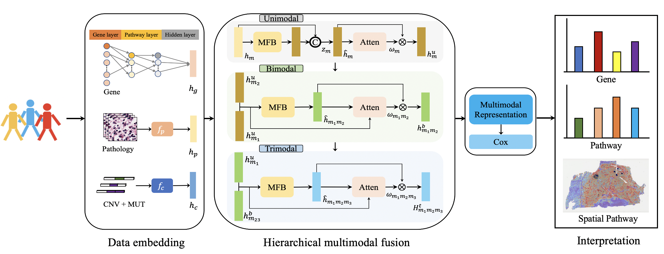
Figure 1: Overview of PONET model.

2 Related Work

Multimodal Fusion. Earlier works on multimodal fusion focus on early fusion and late fusion. Early fusion approaches fuse features by simple concatenation which cannot fully explore intra-modality dynamics (Wöllmer et al., 2013; Poria et al., 2016; Zadeh et al., 2016). In contrast, late fusion fuses different modalities by weighted averaging which fails to model cross-modal interactions (Nojavanasghari et al., 2016; Kampman et al., 2018). The exploitation of relations within each modality has been successfully introduced in cancer prognosis via bilinear model (Wang et al., 2021b) and graph-based model (Subramanian et al., 2021). Adversarial Representation Graph Fusion (ARGF) (Mai et al., 2020) interprets multimodal fusion as a hierarchical interaction learning procedure where firstly bimodal interactions are generated based on unimodal dynamics, and then trimodal dynamics are generated based on bimodal and unimodal dynamics. We propose a new hierarchical fusion framework with modality-specific and cross-modality attentional factorized bilinear modules to mine the comprehensive modality interactions. Our proposed hierarchical fusion framework is different from ARGF in the following ways: 1) We take the sum of the weighted modality-specific representation as the unimodal representation instead of calculating the weighted average of the modality-specific representation in ARGF; 2) For higher level’s fusion, ARGF takes the original embeddings of each modality as input while we use the weighted modality-specific representations; 3) We argue that ARGF takes redundant information during their trimodal dynamics.

Multimodal Survival Analysis. There have been exciting attempts on multimodal fusion of pathology and genomic data for cancer survival prediction (Mobadersany et al., 2018; Cheerla & Gevaert, 2019; Wang et al., 2020). However, these multimodal fusion based methods fail to model the interaction between each subset of multiple modalities explicitly. Kronecker product considers pairwise interactions of two input feature vectors by producing a high-dimensional feature of quadratic expansion (Zadeh et al., 2017), and showed its superiority in cancer survival prediction (Wang et al., 2021b; Chen et al., 2022b; a). Despite promising results, using Kronecker product in multimodal fusion may introduce a large number of parameters that may lead to high computational cost and risk of overfitting (Kim et al., 2017; Liu et al., 2021), thus limiting its applicability and improvement in performance. To overcome this drawback, hierarchical factorized bilinear fusion for cancer survival prediction (HFBSurv) (Li et al., 2022) uses factorized bilinear model to fuse genomic and image features, dramatically reducing computational complexity. PONET differs from HFBSurv in two ways: 1) PONET’s multimodal framework has three levels of hierarchical fusion module including unimodal, bimodal, and trimodal fusion while HFBSurv only considers within-modality and cross-modality fusion which we argue it is not adequate for mining the comprehensive interactions; 2) PONET leverages biological pathway informed network for better prediction and meaningful interpretation purposes.

Pathway-associated Sparse Neural Network. The pathway-based analysis is an approach that a number of studies have investigated to improve both predictive performance and biological interpretability (Jin et al., 2014; Cirillo et al., 2017; Hao et al., 2018; Elmarakeby et al., 2021). Moreover, pathway-based approaches have shown more reproducible analysis results than gene expression data analysis alone (Li et al., 2015; Mallavarapu et al., 2017). These pathway-based deep neural networks can only model genomic data which severely inhibits their applicability in current biomedical research. Additionally, the existing pathway-associated sparse neural network structures are limited for disease mechanism investigation: there is only one pathway layer in PASNet (Hao et al., 2018) which contains limited biological prior information to deep dive into the hierarchical pathway and biological process relationships; P-NET (Elmarakeby et al., 2021) calculates the final prediction by taking the average of all the gene and pathway layers’ outputs, and this will bias the learning process because it will put more weights for some layers’ outputs while underestimating the others.

3 Methodology

3.1 Problem formulation and notations

The model architecture of PONET is presented in Fig. 1, where three modalities are included as input: gene expression $g\in\mathbb{R}^{d_{g}}$, pathological image $p\in\mathbb{R}^{d_{p}}$, and copy number (CNV) + mutation (MUT) $CNV+MUT\in\mathbb{R}^{d_{c}}$, with $d_{p}$ being the dimensionality of $p$ and so on. We define a hierarchical factorized bilinear fusion model for PONET. We build a sparse biological pathway-informed embedding network for gene expression. A fully connected (FC) embedding layer for both preprocessed pathological image feature ($f_{p}$) and the copy number + mutation ($f_{c}$) to map feature into similar embedding space for alleviating the statistical property differences between modalities, the three network architecture details are in Appendix C.1. We label the three modality embeddings as $h_{m}$, $m\in\{g,p,c\}$, the superscript/subscript $u$, $b$, and $t$ represents unimodal fusion, biomodal fusion and trimodal fusion. After that, the embeddings of each modality are first used as input for unimodal fusion to generate the modality-specific representation $h_{m}^{u}=\omega^{m}\hat{h}_{m}$, $\omega^{m}$ represent the modality-specific importance, the feature vector of the unimodal fusion is the sum of all modality-specific representations $h_{u}=\sum_{m}h_{m}^{u}$. In the bimodal fusion, modality-specific representations from the output of unimodal fusion are fused to yield cross-modality representations $h_{m_{1}m_{2}}^{b}=\omega_{m_{1}m_{2}}\hat{h}_{m_{1}m_{2}},m_{1},m_{2}\in\{p,c,g\}$ and $m_{1}\neq m_{2}$, $\omega_{m_{1}m_{2}}$ represents the corresponding cross-modality importance. Similarly, the feature vector of bimodal fusion is calculated as $h_{b}=\sum_{m_{1},m_{2}}h_{m_{1}m_{2}}^{b}$. We propose to build a trimodal fusion to take each cross-modality representation from the output of bimodal fusion to mine the interactions. Similarly to the bimodal fusion architecture, the trimodal fusion feature vector will be $h_{t}=\sum_{m_{1},m_{2},m_{3}}\omega_{m_{1}m_{2}m_{3}}\hat{h}_{m_{1}m_{2}m_{3}},m_{1},m_{2},m_{3}\in\{p,c,g\}$ and $m_{1}\neq m_{2}\neq m_{3}$, $\omega_{m_{1}m_{2}m_{3}}$ represents the corresponding trimodal importance. Finally, PONET concatenates $h_{u}$, $h_{b}$, $h_{t}$ to obtain the final comprehensive multimodal representation and pass it to the Cox proportional hazards model (Cox, 1972; Cheerla & Gevaert, 2019) for survival prediction. In the following sections we will describe our hierarchical factorized bilinear fusion framework, $l$, $o$, $s$ represents the dimensionality of $h_{m}$, $z_{m}$, $\hat{h}_{m1m2}$.

3.2 Sparse network

We design the sparse gene-pathway network consisting of one gene layer followed by three pathway layers. A patient sample of $e$ gene expressions is formed as a column vector, which is denoted by $\mathbf{X}=[x_{1},x_{2},...,x_{e}]$, each node represents one gene. The gene layer is restricted to have connections reflecting the gene-pathway relationships curated by the Reactome pathway dataset (Fabregat et al., 2020). The connections are encoded by a binary matrix $\mathbf{M}\in\mathbb{R}^{a\times e}$, where $a$ is the number of pathways and $e$ is the number of genes, an element of $\mathbf{M}$, $m_{ij}$, is set to one if gene $j$ belongs to pathway $i$. The connections that do not exist in the Reactome pathway dataset will be zero-out. For the following pathway-pathway layers, a similar scheme is applied to control the connection between consecutive layers to reflect the parent-child hierarchical relationships that exist in the Reactome dataset. The output of each layer is calculated as

$$y=f[(\mathbf{M}*\mathbf{W})^{T}\mathbf{X}+\mathbf{\epsilon}]$$ (1)

where $f$ is the activation function, $\mathbf{M}$ represents the binary matrix, $\mathbf{W}$ is the weights matrix, $\mathbf{X}$ is the input matrix, $\mathbf{\epsilon}$ is the bias vector, and $*$ is the Hadamard product. We use tanh for the activation of each node. We allow the information flow from the biological prior informed network starting from the first gene layer to the last pathway layer, and we label the last layer output embeddings of the sparse network for gene expression as $h_{g}$.

3.3 unimodal fusion

Bilinear models (Tenenbaum & Freeman, 2000) provide richer representations than linear models. Given two feature vectors in different modalities, e.g., the visual features $x\in\mathbb{R}^{m\times 1}$ for an image and the genomic features $y\in\mathbb{R}^{n\times 1}$ for a genomic profile, the bilinear model uses a quadratic expansion of linear transformation considering every pair of features:

$$z_{i}=x^{T}W_{i}y$$ (2)

where $W_{i}\in\mathbb{R}^{m\times n}$ is a projection matrix, $z_{i}\in\mathbb{R}$ is the output of the bilinear model. Bilinear models introduce a large number of parameters which potentially lead to high computational cost and overfitting risk. To address these issues, Yu et al. (2017) develop the Multi-modal Factorized Bilinear pooling (MFB) method, which enjoys the dual benefits of compact output features and robust expressive capacity.

Inspired by the MFB (Yu et al., 2017) and its application in pathology and genomic multimodal learning (Li et al., 2022), we propose unimodal fusion to capture modality-specific representations and quantify their importance. The unimodal fusion takes the embedding of each modality $h_{m}$ as input and factorizes the projection matrix $W_{i}$ in Eq. (2) as two low-rank matrices:

$$\begin{array}[]{rcl}z_{i}&=&h_{m}^{T}W_{i}h_{m}=\sum\limits_{d=1}^{k}h_{m}^{T}u_{m,d}v_{m,d}^{T}h_{m}\\ &=&1^{T}(U_{m,i}^{T}h_{m}\circ V_{m,i}^{T}h_{m}),m\in\{p,c,g\}\end{array}$$ (3)

we get the output feature $z_{m}$:

$$z_{m}=\operatorname{SumPooling}\left(\tilde{U}_{m}^{T}h_{m}{}{\circ}\tilde{V}_{m}^{T}h_{m},k\right),m\in\{p,c,g\}$$ (4)

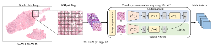
Figure 2: Overall framework of the visual representation extraction using pre-trained self-supervised vision transformer.

where $k$ is the latent dimensionality of the factorized matrices. SumPooling $(x,k)$ function performs sum pooling over $x$ by using a 1-D non-overlapped window with the size $\mathrm{k},\tilde{U}_{m}\in\mathbb{R}^{l\times ko}$ and $\tilde{V}_{m}\in\mathbb{R}^{l\times ko}$ are 2-D matrices reshaped from $U_{m}$ and $V_{m}$, $U_{m}=$$\left[U_{m,1},\ldots,U_{m,h}\right]\in\mathbb{R}^{l\times k\times o}$ and $V_{m}=\left[V_{m,1},\ldots,V_{m,h}\right]\in\mathbb{R}^{l\times k\times o}$. Each modality-specific representation $\hat{h}_{m}\in\mathbb{R}^{l+o}$ is obtained as:

$$\hat{h}_{m}=h_{m}\text{\copyright}z_{m},m\in\{p,c,g\}$$ (5)

where $\copyright$ denotes vector concatenation. We also introduce a modality attention network $Atten\in\mathbb{R}^{l+o}\rightarrow\mathbb{R}^{1}$ to determine the weight for each modality-specific representation to quantify its importance:

$$\omega_{m}=Atten(\hat{h}_{m};\Theta_{Atten}),m\in\{p,c,g\}$$ (6)

where $\omega_{m}$ is the weight of modality $m$. In practice, $Atten$ consists of a sigmoid activated dense layer parameterized by $\Theta_{Atten}$. Therefore, the output of each modality in unimodal fusion, ${h}_{m}^{u}$, is denoted as $\omega_{m}\hat{h}_{m}\in\mathbb{R}^{l+o},m\in\{p,c,g\}$. Accordingly, the output of unimodal fusion, $h_{u}$, is the sum of each weighted modality-specific representation $\omega_{m}\hat{h}_{m},m\in\{p,c,g\}$ which is different from ARGF (Mai et al., 2020) that used the weighted average of different modalities as the unimodal fusion output.

3.4 bimodal and trimodal fusion

Bimodal fusion aims to fuse diverse information of different modalities and quantify different importance for them. After receiving the modality-specific representations ${h}_{m}^{u}$ from the unimodal fusion, we can generate the cross-modality representation $\hat{h}_{m_{1}m_{2}}\in\mathbb{R}^{s}$ similar to Eq. (4) :

$$\begin{gathered}\hat{h}_{m1,m2}=\operatorname{Sum}\operatorname{Pooling}\left(\tilde{U}_{m_{1}}^{T}h_{m_{1}}^{u}{}{\circ}\tilde{V}_{m_{2}}^{T}h_{m_{2}}^{u},k\right),\\ m_{1},m_{2}\in\{p,c,g\},m_{1}\neq m_{2}\end{gathered}$$ (7)

where $\quad\tilde{U}_{m_{1}}^{T}\in\mathbb{R}^{(l+o)\times ks}$ and $\tilde{V}_{m_{2}}^{T}\in\mathbb{R}^{(l+o)\times ks}$ are 2-D matrices reshaped from $U_{m_{1}}$ and $V_{m_{2}}$ and $U_{m_{1}}=\left[U_{m_{1},1},\ldots,U_{m_{1},s}\right]\in\mathbb{R}^{(l+o)\times k\times s}$ and $V_{m_{2}}=\left[V_{m_{2},1},\ldots,V_{m_{2},s}\right]\in\mathbb{R}^{(l+o)\times k\times s}$. We leverage a bimodal attention network (Mai et al., 2020) to identify the importance of the cross-modality representation. The similarity $S_{m_{1}m_{2}}\in\mathbb{R}^{1}$ of $h_{m_{1}}^{u}$ and $h_{m_{2}}^{u}$ is first estimated as follows:

$$S_{m_{1},m_{2}}=\sum_{i=1}^{l+o}\left(\frac{e^{\omega_{m_{1}}}h_{m_{1},i}^{u}}{\sum_{j=1}^{l+o}e^{\omega_{m_{1}}h_{m_{1},j}^{u}}}\right)\left(\frac{e^{\omega_{m_{2}}h_{m_{2},i}^{u}}}{\sum_{j=1}^{l+o}e^{\omega_{m_{2}}h_{m_{2},j}^{u}}}\right)$$ (8)

where the computed similarity is in the range of 0 to 1. Then, the cross-modality importance $\omega_{m_{1}m_{2}}$ is obtained by:

$$\omega_{m_{1}m_{2}}=\frac{e^{\hat{\omega}_{m_{i}m_{j}}}}{\sum_{m_{i}\neq m_{j}}e^{\hat{\omega}_{m_{i}m_{j}}}},\hat{\omega}_{m_{1}m_{2}}=\frac{\omega_{m_{1}}+\omega_{m_{2}}}{S_{m_{1}m_{2}}+S_{0}}$$ (9)

where $S_{0}$ represents a pre-defined term controlling the relative contribution of similarity and modality-specific importance, and here is set to $0.5$. Therefore, the output of bimodal fusion, $h_{b}$, is the sum of each weighted cross-modality representation $\omega_{m_{1}m_{2}}\hat{h}_{m_{1}m_{2}},m_{1},m_{2}\in\{p,c,g\}$ and $m_{1}\neq m_{2}$.

In trimodal fusion, each bimodal fusion output is fused with the unimodal fusion output that does not contribute to the formation of the bimodal fusion. The output for each corresponding trimodal representation is $\hat{h}_{m_{1}m_{2}m_{3}}$. In addition, trimodal attention was applied to identify the importance of each trimodal representation, $\omega_{m_{1}m_{2}m_{3}}$. The output of the trimodal fusion, $h_{t}$, is the sum of each weighted trimodal representation $\omega_{m_{1}m_{2}m_{3}}\hat{h}_{m_{1}m_{2}m_{3}},m_{1},m_{2},m_{3}\in\{p,c,g\}$ and $m_{1}\neq m_{2}\neq m_{3}$.

3.5 Survival Loss Function

We train the model through the Cox partial likelihood loss (Cheerla & Gevaert, 2019) with $l_{1}$ regularization for survival prediction, which is defined as:

$$\ell(\Theta)=-\sum_{i:E_{i}=1}\left(\hat{\mathfrak{h}}_{\Theta}\left(x_{i}\right)-\log\sum_{j:T_{i}>T_{j}}\exp\left(\hat{\mathfrak{h}}_{\Theta}\left(x_{j}\right)\right)\right)+\lambda\left(\|\Theta\|_{1}\right)$$ (10)

where the values $E_{i},T_{i}$ and $x_{i}$ for each patient represent the survival status, the survival time, and the feature, respectively. $E_{i}$ = 1 means event while $E_{i}$ = 0 represents censor. $\hat{\mathfrak{h}}_{\Theta}$ is the neural network model trained for predicting the risk of survival, $\Theta$ is the neural network model parameters, and $\lambda$ is a regularization hyperparameter to avoid overfitting.

4 Experiments

4.1 Experimental Setup

Datasets. To validate our proposed method, we used six cancer datasets from The Cancer Genome Atlas (TCGA), a public cancer data consortium that contains matched diagnostic WSIs and genomic data with labeled survival times and censorship statuses. The genomic profile features (mutation status, copy number variation, RNA-Seq expression) are preprocessed by Porpoise (Chen et al., 2022b). For this study, we used the following cancer types: Bladder Urothelial Carcinoma (BLCA) (n = 437), Kidney Renal Clear Cell Carcinoma (KIRC) (n = 350), Kidney Renal Papillary Cell Carcinoma (KIRP) (n = 284), Lung Adenocarcinoma (LUAD) (n = 515), Lung Squamous Cell Carcinoma (LUSC) (n = 484), Pancreatic adenocarcinoma (PAAD) (n = 180). We downloaded the same diagnostic WSIs from the TCGA website that were used in Porpoise study to match the paired genomic features and survival times. The feature alignment table for all the cancer types is in Appendix 4. For each WSI, automated segmentation of tissue was performed. Following segmentation, image patches of size 224 $\times$ 224 were extracted without overlap at the 20 X equivalent pyramid level from all tissue regions identified while excluding the white background and selecting only patches with at least 50% tissue regions. Subsequently, a visual representation of those patches is extracted with a vision transformer (Wang et al., 2021a) pre-trained on the TCGA dataset through a self-supervised constructive learning approach, such that each patch is represented as a 1 $\times$ 2048 vector. Fig. 2 shows the framework for the visual representation extraction by vision transformer (VIT). Survival outcome information is available at the patient level, we aggregated the patch-level feature into slide level feature representations based on an attention-based method (Lu et al., 2021; Ilse et al., 2018).

Baselines. Using the same 5-fold cross-validation splits for evaluating PONET, we implemented and evaluated six state-of-the-art methods for survival outcome prediction. Additionally, we included three variations of PONET: a) PONET-O represents only genomic data, and pathway architecture for the gene expression are included in the model; b) PONET-OH represents only genomic and pathological image data but without pathway architecture in the model; c) PONET is our full model. For all methods, we use the same VIT feature extraction pipeline for WSIs, as well as identical training hyperparameters and loss functions for supervision. Training details and the parameters tuning can be found in Appendix C.2.

CoxPH (Cox, 1972) represents the standard Cox proportional hazard models.
DeepSurv (Katzman et al., 2018) is the deep neural network version of the CoxPH model.
Pathomic Fusion (Chen et al., 2022a) as a pioneered deep learning-based framework for predicting survival outcomes by fusing pathology and genomic multimodal data, in which Kronecker product is taken to model pairwise feature interactions across modalities.
GPDBN (Wang et al., 2021b) adopts Kronecker product to model inter-modality and intra-modality relations between pathology and genomic data for cancer prognosis prediction.
HFBSurv (Li et al., 2022) extended GPDBN using the factorized bilinear model to fuse genomic and pathology features in a within-modality and cross-modalities hierarchical fusion.
Porpoise (Chen et al., 2022b) applied the discrete survival model and Kronecker product to fuse pathology and genomic data for survival prediction (Zadeh & Schmid, 2020).

Evaluation. For each cancer dataset, we used the cross-validated concordance index (C-Index) (Appendix B.1) (Harrell et al., 1982) to measure the predictive performance of correctly ranking the predicted patient risk scores with respect to overall survival.

4.2 Results

Comparison with Baselines. In combing pathology image, genomics, and pathway network via PONET, our approach outperforms CoxPH models, unimodal networks, and previous deep learning-based approaches on pathology-genomic-based survival outcome prediction (Table 1). The results show that deep learning-based approaches generally perform better than the CoxPH model. PONET achieves superior C-index values in all six cancer types. All versions of PONET outperform Pathomic Fusion by a big margin. Pathomic Fusion uses Kronecker product to fuse the two modalities, and that’s also the reason why other advanced fusion methods, like GPDBN and HFBSurv, achieve better performance. Also, we argue that Pathomic Fusion extracts the region of interest of pathology image for feature extraction might limit the understanding of the tumor microenvironment of the whole slide. HFBSurv shows better performance than GPDBN and Pathomic Fusion which is consistent with their findings, and these results further demonstrate that the hierarchical factorized bilinear model can better mine the rich complementary information among different modalities compared to the Kronecker product. Porpoise performs similarly with PONET on TCGA-KIRC and TCGA-KIRP and outperformed HFBSurv in these two studies, this probably is due to Porpoise partitioned the survival time into different non-overlapping bins and parameterized it as a discrete survival model (Zadeh & Schmid, 2020) which works better for these two cancer types. In other cases, Porpoise performs similarly to HFBSurv. Note: the results of Porpoise are from their paper (Chen et al., 2022b).

Additionally, we can see that PONET consistently outperforms PONET-O and PONET-OH indicating the effectiveness of the biological pathway-informed neural network and the contribution of pathological image for the overall survival prediction.

Table 1: C-Index (mean $\pm$ standard deviation) of PONET and ablation experiments in TCGA survival prediction. The top two performers are highlighted in bold.

Model	TCGA-BLCA	TCGA-KIRC	TCGA-KIRP	TCGA-LUAD	TCGA-LUSC	TCGA-PAAD
CoxPH (Age + Gender) (Cox, 1972)	0.525 $\pm$ 0.130	0.550 $\pm$ 0.070	0.544 $\pm$ 0.050	0.531 $\pm$ 0.082	0.532 $\pm$ 0.094	0.539 $\pm$ 0.092
DeepSurv (Kampman et al., 2018)	0.580 $\pm$ 0.062	0.620 $\pm$ 0.043	0.560$\pm$ 0.063	0.534 $\pm$0.077	0.541 $\pm$ 0.066	0.544 $\pm$ 0.076
GPDBN (Wang et al., 2021b)	0.612 $\pm$ 0.042	0.647 $\pm$ 0.073	0.669 $\pm$ 0.109	0.565 $\pm$ 0.057	0.545 $\pm$ 0.063	0.571 $\pm$ 0.060
HFBSurv (Li et al., 2022)	0.622 $\pm$ 0.043	0.667 $\pm$ 0.053	0.769 $\pm$ 0.109	0.581 $\pm$ 0.017	0.548 $\pm$ 0.049	0.591 $\pm$ 0.052
Pathomic Fusion (Chen et al., 2022a)	0.586 $\pm$ 0.062	0.598 $\pm$ 0.060	0.577 $\pm$ 0.032	0.543 $\pm$ 0.065	0.523 $\pm$0.045	0.545 $\pm$ 0.064
Porpoise (Chen et al., 2022b)	0.617 $\pm$ 0.048	0.711 $\pm$ 0.051	0.811 $\pm$ 0.089	0.586 $\pm$0.056	0.527 $\pm$ 0.043	0.591 $\pm$ 0.064
PONET-O (ours)	0.596 $\pm$ 0.056	0.664 $\pm$ 0.056	0.761 $\pm$ 0.093	0.623 $\pm$0.062	0.538 $\pm$ 0.037	0.598 $\pm$ 0.027
PONET-OH (ours)	0.625 $\pm$ 0.063	0.695 $\pm$ 0.043	0.776 $\pm$ 0.123	0.618 $\pm$ 0.049	0.553 $\pm$ 0.049	0.591 $\pm$ 0.050
PONET (ours)	0.643 $\pm$ 0.037	0.726 $\pm$ 0.056	0.829 $\pm$ 0.054	0.646 $\pm$0.047	0.567 $\pm$ 0.066	0.639 $\pm$ 0.080

Ablation Studies. To assess whether the impact of hierarchical factorized bilinear fusion strategy is indeed effective, we compare PONET with four single-fusion methods: 1) Simple concatenation: concatenate each modality embeddings; 2) Element-wise addition: element-wise addition from each modality embeddings; 3) Tensor fusion (Zadeh et al., 2017): Kronecker product from each modality embeddings. Table 2 shows the C-index values of different methods. We can see that PONET achieves the best performance and shows remarkable improvement over single-fusion methods on different cancer type datasets. For example, PONET outperforms the Simple concatenation by 8.4% (TCGA-BLCA), 27% (TCGA-KIRP), 15% (TCGA-LUAD), 8.0% (TCGA-LUSC), and 11.4% (TCGA-PAAD), etc.

Table 2: Evaluation of PONET on different fusion methods and pathway designs by C-index (mean $\pm$ standard deviation). The best performer is highlighted in bold.

	Methods	TCGA-BLCA	TCGA-KIRP	TCGA-LUAD	TCGA-LUSC	TCGA-PAAD
Single fusion	Simple concatenation	0.585 $\pm$ 0.045	0.652 $\pm$ 0.049	0.554 $\pm$ 0.065	0.525 $\pm$ 0.066	0.568 $\pm$ 0.075
	Element-wise addition	0.592 $\pm$ 0.047	0.655 $\pm$ 0.055	0.587 $\pm$ 0.065	0.522 $\pm$ 0.046	0.588 $\pm$ 0.055
	Tensor fusion (Zadeh et al., 2017)	0.605 $\pm$ 0.046	0.775 $\pm$ 0.053	0.595 $\pm$ 0.060	0.545 $\pm$ 0.045	0.592 $\pm$ 0.061
Hierarchical fusion	Unimodal	0.596 $\pm$ 0.035	0.783 $\pm$ 0.063	0.611 $\pm$ 0.056	0.553 $\pm$ 0.073	0.595 $\pm$ 0.053
	Bimodal	0.602 $\pm$ 0.062	0.789 $\pm$ 0.053	0.601 $\pm$ 0.056	0.552 $\pm$ 0.051	0.598 $\pm$ 0.083
	ARGF (Mai et al., 2020)	0.597 $\pm$ 0.054	0.792 $\pm$ 0.043	0.614 $\pm$ 0.051	0.556 $\pm$ 0.063	0.602 $\pm$ 0.065
	Unimodal + Bimodal	0.614 $\pm$ 0.052	0.803 $\pm$ 0.061	0.631 $\pm$ 0.044	0.578 $\pm$ 0.058	0.615 $\pm$ 0.057
Pathway design	PASNet (Hao et al., 2018)	0.606 $\pm$ 0.045	0.793 $\pm$ 0.051	0.621 $\pm$ 0.061	0.551 $\pm$ 0.069	0.625 $\pm$ 0.057
	P-NET (Elmarakeby et al., 2021)	0.622 $\pm$ 0.047	0.802 $\pm$ 0.071	0.625 $\pm$ 0.045	0.562 $\pm$ 0.054	0.627 $\pm$ 0.073
	PONET	0.643 $\pm$ 0.037	0.829 $\pm$ 0.054	0.641 $\pm$ 0.046	0.567 $\pm$ 0.066	0.639 $\pm$ 0.070

Furthermore, we adopted five different configurations of PONET to evaluate each hierarchical component of the proposed method: 1) Unimodal: unimodal fusion output as the final feature representation; 2) Bimodal: bimodal fusion output as the final feature representation; 3) Unimodal + Bimodal: hierarchical (include both unimodal and bimodal feature representation) fusion; 4) ARGF: ARGF (Mai et al., 2020) fusion strategy; 5) PONET: our proposed hierarchical strategy by incorporating unimodal, bimodal, and trimodal fusion output. As shown in Table 2, Unimodal + Bimodal performs better than Unimodal and Bimodal which demonstrates that Unimodal + Bimodal can capture the relations within each modality and across modalities. ARGF performs worse than Unimodal + Bimodal and far worse than PONET across all the cancer types. PONET outperforms Unimodal + Bimodal in 4 out of 5 cancer types indicating that three layers of hierarchical fusion can mine the comprehensive interactions among different modalities.

To evaluate our sparse gene-pathway network design, we compare PONET with PASNet (Hao et al., 2018) and P-NET (Elmarakeby et al., 2021) pathway architecture, PASNet performs the worst due to the fact that it only has one pathway layer in the network, and thus limited prior information was used to predict the outcome. PONET constantly outperforms P-NET across all the cancer types, which demonstrates that averaging all the intermediate layers’ output for the final prediction cannot fully capture the prior information flow among the hierarchical biological structures.

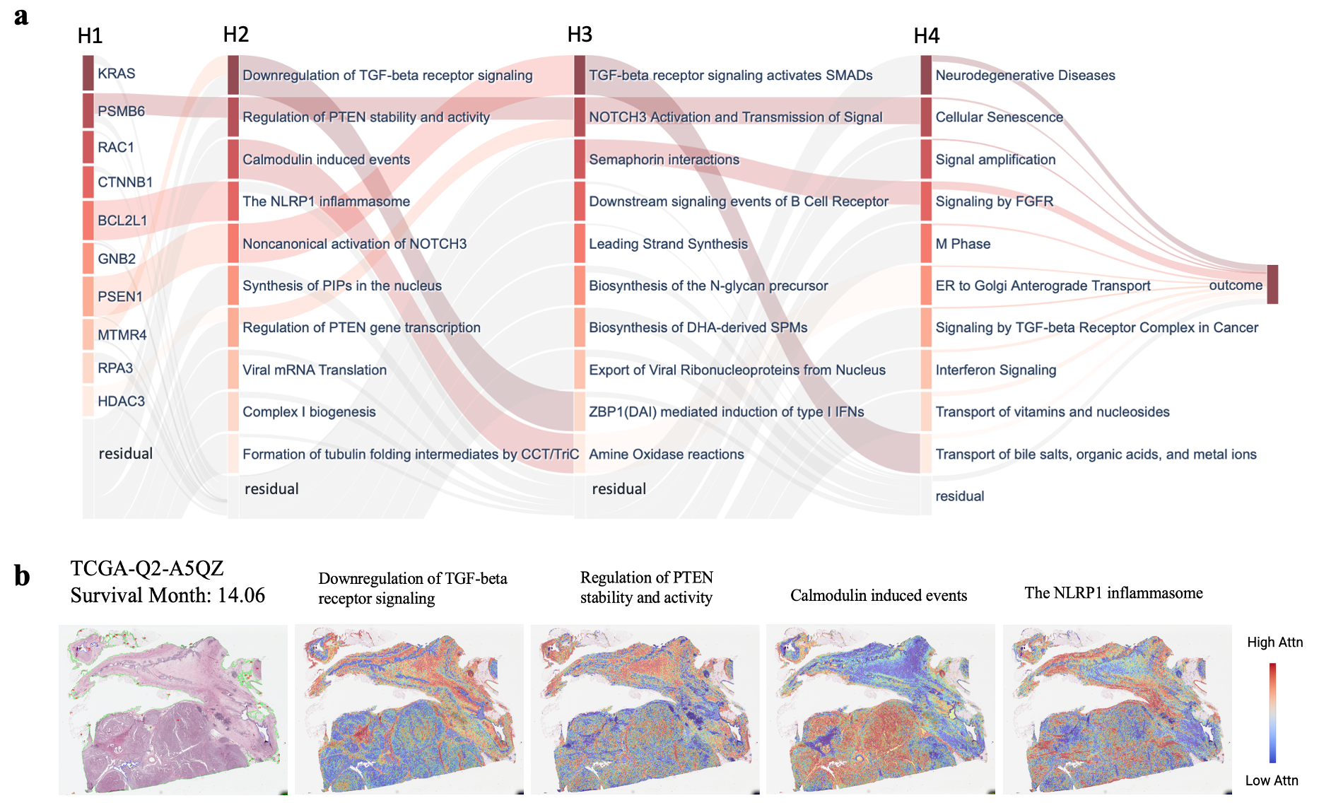
Figure 3: Inspecting and interpreting PONET on TCGA-KIRP. a: Sankey diagram visualization of inner layers of PONET shows the estimated relative importance of different nodes in each layer. Nodes in the first layer represent genes; the next layers represent pathways; and the final layer represents the model outcome. Different layers are linked by weights. Nodes with darker colors are more important, while transparent nodes represent the residual importance of undisplayed nodes in each layer, H1 presents the gene layer, and H2-H4 represent pathway layers; b: Co-attention visualization of top 4 ranked pathways in one case of TCGA-KIRP.

Model Interpretation. We discuss the model interpretation results for cancer type TCGA-KIRP here and the results for other cancer types are included in the Appendix C.3. To understand the interactions between different genes, pathways, and biological processes that contributed to the predictive performance and to study the paths of impact from the input to the outcome, we visualized the whole structure of PONET with the fully interpretable layers after training (Fig. 3 a). To evaluate the relative importance of specific genes contributing to the model prediction, we inspected the genes layer and used the Integrated Gradients attribution (Sundararajan et al., 2017) method to obtain the total importance score of genes, and the modified ranking algorithm details are included in the Appendix B.3. Highly ranked genes included KRAS, PSMB6, RAC1, and CTNNB1 which are known kidney cancer drivers previously (Yang et al., 2017; Shan et al., 2017; Al-Obaidy et al., 2020; Guo et al., 2022). GBN2, a member of the guanine nucleotide-binding proteins family, has been reported that the decrease of its expression reduced tumor cell proliferation (Zhang et al., 2019). A recent study identified a strong dependency on BCL2L1, which encodes the BCL-XL anti-apoptotic protein, in a subset of kidney cancer cells (Grubb et al., 2022). This biological interpretability revealed established and novel molecular features contributing to kidney cancer. In addition, PONET selected a hierarchy of pathways relevant to the model prediction, including downregulation of TGF-$\beta$ receptor signaling, regulation of PTEN stability and activity, the NLRP1 inflammasome, and noncanonical activation of NOTCH3 by PSEN1, PSMB6, and BCL2L1. TGF-$\beta$ signaling is increasingly recognized as a key driver in cancer, and in progressive cancer tissues TGF-$\beta$ promotes tumor formation, and its increased expression often correlates with cancer malignancy (Han et al., 2018). Noncanonical activation of NOTCH3 was reported to limit tumor angiogenesis and plays a vital role in kidney disease (Lin et al., 2017).

To further inspect the pathway spatial association with the WSI slide we adopted the co-attention survival method MCAT (Chen et al., 2021) between WSIs and genomic features on the top pathways of the second layer, visualized as a WSI-level attention heatmap for each pathway genomic embedding in Fig. 3 b (algorithm details are included in the Appendix B.4). We used the gene list from the top 4 pathways as the genomic features and trained MCAT on the TCGA-KIRP dataset for survival prediction. Overall, we observe that high attention in different pathways showed different spatial pattern associations with the slide. This heatmap can reflect genotype-phenotype relationships in cancer pathology. The high attention regions (red) of different pathways in the heatmap have positive associations with the predicted death risk while the low attention regions (blue) have negative associations with the predicted risk. By further checking the cell types in high attention patches we can gain insights of prognostic morphological determinants and have a better understanding of the complex tumor microenvironment.

Table 3: Comparison of model complexity

Methods	Number of Parameters	FLOPS
Pathomic Fusion	175M	168G
GPDBN	82M	91G
HFBSurv	0.3M	0.5G
PONET	2.8M	3.1G

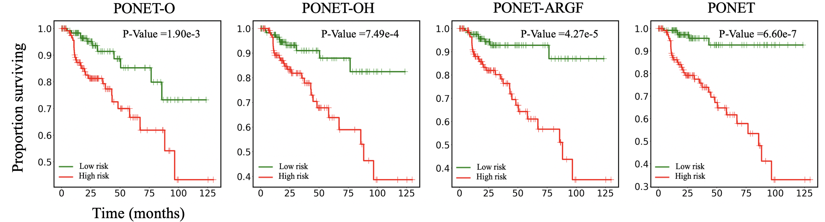
Figure 4: Kaplan-Meier analysis of patient stratification of low and high risk patients via four variations of PONET on TCGA-KIRP. Low and high risks are defined by the median 50$\%$ percentile of hazard predictions via each model prediction. Log-rank test was used to test for statistical significance in survival distributions between low and high risk patients.

Patient Stratification. In visualizing the Kaplan-Meier survival curves of predicted high risk and low risk patient populations, we plot four variations of PONET in Fig. 4. PONET-ARGF represents the model that we use the hierarchical fusion strategy of ARGF in our pathway-informed PONET model. From the results, PONET enables easy separation of patients into low and high risk groups with remarkably better stratification (P-Value = 6.60e-7) in comparison to the others.

Complexity Comparison. We compared PONET with Pathomic Fusion, GPDBN, and HFBSurv since both Pathomic Fusion and GPDBN are based on Kronecker product to fuse different modalities while GPDBN and HFBSurv modeled inter-modality and intra-modality relations which have similar consideration to our method. As illustrated in Table 3, PONET has 2.8M (M = Million) trainable parameters, which is approximately 1.6%, 3.4%, and 900% of the number of parameters of Pathomic Fusion, GPDBN, and HFBSurv. To assess the time complexity of PONET and the competitive methods, we calculate each method’s floating-point operations per second (FLOPS) in testing. The results in Table 3 show that PONET needs 3.1G during testing, compared with 168G, 91G, and 0.5G in Pathomic Fusion, GPDBN, and HFBSurv. The main reason for fewer trainable parameters and the number of FLOPS lies in that PONET and HFBSurv perform multimodal fusion using the factorized bilinear model, and can significantly reduce the computational complexity and meanwhile obtain more favorable performance. PONET has one additional trimodal fusion which explains why it has more trainable parameters than HFBSurv.

5 Conclusion

In this study, we pioneer propose a novel biological pathway-informed hierarchical multimodal fusion model that integrates pathology image and genomic profile data for cancer prognosis. In comparison to previous works, PONET deeply mines the interaction from multimodal data by conducting unimodal, bimodal and trimodal fusion step by step. Empirically, PONET demonstrates the effectiveness of the model architecture and the pathway-informed network for superior predictive performance. Specifically, PONET provides insight on how to train biologically informed deep networks on multimodal biomedical data for biological discovery in clinic genomic contexts which will be useful for other problems in medicine that seek to combine heterogeneous data streams for understanding diseases and predicting response and resistance to treatment.

Appendix A Data

Table 3 in Appendix 4 shows the number of patients with matched different data modalities: WSI (Whole slide image), CNV (Copy number), MUT (Mutation), RNA (RNA-Seq gene expression). For each TCGA dataset and each patient we have preprocessed data dimensions $\mathbf{d}_{\mathrm{g}}\in\mathbb{R}^{1\times 2000}$ (RNA), $\mathbf{d}_{\mathrm{c}}\in\mathbb{R}^{1\times 227}$ (CNV + MUT), and $\mathbf{d}_{\mathrm{p}}\in\mathbb{R}^{1\times 32}$ (WSI) which will be used for our multimodal fusion.

Table 4: TCGA Data Feature Alignment Summary

	WSI	CNV	MUT	RNA	WSI+CNV+MUT	WSI+MUT+RNA	ALL
Cancer Type
BLCA	454	443	452	450	441	448	437
KIRC	517	509	357	514	352	355	350
KIRP	294	291	286	293	284	285	284
LUAD	528	522	523	522	519	519	515
LUSC	505	502	489	503	486	487	484
PAAD	208	201	187	195	187	180	180

Appendix B Methods

B.1 C-Index

We use concordance-index (C-index) (Harrell et al., 1982) to measure the performance of survival models. It evaluates the model by measuring the concordance of the ranking of predicted harzards with the true survival time of patients. The range of the $\mathrm{C}$-index is $[0,1]$, and larger values indicate better performance with a random guess leading to a $\mathrm{C}$-index of $0.5$.

B.2 WSI representation learning

It has been shown that the WSI visual representations extracted by self-supervised learning methods on histopathological images are more accurate and transferable than the supervised baseline models on domain-irrelevant datasets such as ImageNet. In this work, a pre-trained Vision Transformer (ViT) model (Wang et al., 2021a) that is trained on a large histopathological image dataset has been utilized for tile feature extraction. The model is composed of two main neural networks that learn from each other, i.e., student and teacher networks. Parameters of the teacher model $\theta_{t}$ are updated using the student network with parameter $\theta_{s}$ using the update rule represented in Eq. (11).

$$\theta_{t}\leftarrow\tau\theta_{t}+(1-\tau)\theta_{s}$$ (11)

Two different views of a given input H&E image ${x}$, uniformly selected from the training set $\mathcal{I}$, are generated using random augmentations, i.e., ${u}$, ${v}$. Then, student and teacher models generate two different visual representations according to ${u}$ and ${v}$ as $y_{1}=f^{\theta_{s}}\left({u}\right)$ and $\hat{y}_{2}=f^{\theta_{t}}\left({v}\right)$, respectively. Finally, the generated visual representations are transformed into latent space using linear projection as $p_{1}=g^{\theta_{s}}\left(g^{\theta_{s}}\left(y_{1}\right)\right)$ and $\hat{z_{2}}=g^{\theta_{t}}\left(\hat{y}_{2}\right)$ for student and teacher networks, respectively. Similarly, feeding ${v}$ and ${u}$ to student and teacher networks leads to $y_{2}=f^{\theta_{s}}\left({v}\right),\hat{y_{1}}=f^{\theta_{t}}\left({u}\right),p_{2}=g^{\theta_{s}}\left(g^{\theta_{s}}\left(y_{2}\right)\right)$ and $\hat{z_{1}}=g^{\theta_{t}}\left(\hat{y_{1}}\right)$. Finally, the symmetric objective function $L_{loss}$ is optimized through minimizing the $\ell_{2}-\text{norm}$ distance between student and teacher as Eq. (12)

$$L_{loss}=\frac{1}{2}L\left(p_{1},\hat{z}_{2}\right)+\frac{1}{2}L\left(p_{2},\hat{z}_{1}\right)$$ (12)

where $L(p,z)=-\frac{p}{\|p\|_{2}}\cdot\frac{z}{\|z\|_{2}}$ and $\|\cdot\|_{2}$ represents $\ell_{2}-\text{norm}$.

B.3 Sparse network feature interpretation

We use the Integrated Gradients attribution algorithm to rank the features in all layers. Inspired by PNET (Elmarakeby et al., 2021), to reduce the bias introduced by over-annotation of certain nodes (nodes that are members of too many pathways), we adjusted the Integrated Gradients scores using a graph informed function $f$ that considers the connectivity of each node. The importance score of each node $i$, $C_{i}^{l}$ is divided by the node degree $d_{i}^{l}$ if the node degree is larger than the mean of node degrees plus $5\sigma$ where $\sigma$ is the standard deviation of node degrees.

$$d_{i}^{l}=fan-in_{i}^{l}+fan-out_{i}^{l}$$

adjusted $C_{i}^{l}=f(x)=\begin{cases}\frac{C_{i}^{l}}{d_{i}^{l}},&d_{i}^{l}>\mu+5\sigma\\ C_{i}^{l},&\text{ otherwise }\end{cases}$

B.4 Co-attention based pathway visualization

After we got the ranking of top genes and pathways, we adopted the co-attention survival model (MCAT) (Chen et al., 2021) to show the spatial visualization of genomic features. We trained MACT on all our TCGA datasets, and MACT learns how WSI patches attend to genes when predicting patient survival. We define each WSI patch representation and pathway genomic features as $H_{bag}$ and $G_{bag}$. The genomic features are the gene list values from the top pathways of each TCGA dataset. The model uses $G_{bag}\in\mathbb{R}^{N\times d_{g}}$ to guide the feature aggregation of $H_{bag}\in\mathbb{R}^{N\times d_{p}}$ into a clustered set of gene-guided visual concepts $\widehat{H}_{\text{bag }}\in\mathbb{R}^{N\times d_{p}}$ , $d_{g}$ and $d_{p}$ represents the dimension for the pathway (number of genes involved in the pathway) and patch. Through the following mapping:

$$\operatorname{CoAttn}_{G\rightarrow H}(G,H)=\operatorname{softmax}\left(\frac{QK^{\top}}{\sqrt{d_{p}}}\right)$$

$$=\operatorname{softmax}\left(\frac{\mathbf{W}_{q}GH^{\top}\mathbf{W}_{s}^{\top}}{\sqrt{d_{p}}}\right)\mathbf{W}_{v}H\rightarrow A_{\text{coattn }}\mathbf{W}_{v}H\rightarrow\widehat{H}$$

where $\mathbf{W}_{q},\mathbf{W}_{s},\mathbf{W}_{v}\in\mathbb{R}^{d_{p}\times d_{p}}$ are trainable weight matrices multiplied to the queries $G_{\text{bag }}$ and key-value pair ($H_{\text{bag }},H_{\text{bag }}$), and $A_{\text{coattn }}\in\mathbb{R}^{N\times M}$ is the co-attention matrix for computing the weighted average of $H_{\text{bag }}$. Here, $M$ represents the number of patches in one slide, and $N$ represents the number of pathways (We trained the top four pathways, so $N=4$ in our study).

Appendix C Experiments

C.1 Network architecture

Sparse network for gene: The final gene expression embedding is $\mathbf{h}_{\mathrm{g}}\in\mathbb{R}^{1\times 50}$.

Pathology network: The slide level image feature representation is passed through an image embedding layer and encodes the embedding as $\mathbf{h}_{\mathrm{p}}\in\mathbb{R}^{1\times 50}$.

CNV + MUT network: Similarly as the pathology network, the patient level CNV + MUT feature representation is passed through an FC embedding layer and encodes the embedding as $\mathbf{h}_{\mathrm{c}}\in\mathbb{R}^{1\times 50}$.

C.2 Experimental Details

PONET. The latent dimensionality of the factorized matrices $k$ is a very important tuning parameter. We tune $k=[3,5,10,20,30,50]$ based on the testing C-index value (Appendix Fig. 5) and the loss of training and testing plot (Appendix Fig. 6) for each dataset. We choose $k$ to maximize the C-index value and also it should have stable convergence in both training and testing loss. For example, we choose $k=10$ in TCGA-KIRP for the optimized results. We can see that in Appendix Fig. 5 the testing loss is quite volatile when $k$ is less than 10. Similarly, we choose $k=[20,10,20,20,10]$ for TCGA-BLCA, TCGA-KIRC, TCGA-LUAD, TCGA-LUSC, and TCGA-PAAD, respectively.

The learning rate and the regularization hyperparameter $\lambda$ for the Cox partial likelihood loss are also tunable parameters. The model is trained with Adam optimizer. For each training/testing pair, we first empirically preset the learning rate to 1.2e-4 as a starting point for a grid search during training, the optimal learning rate is determined through the 5-fold cross-validation on the training set, C-index was used for the performance metric. After that, the model is trained on all the training sets and evaluated on the testing set. We use 2e-3 through the experiments for $\lambda$. The batch size is set to 16, and the epoch is 100. During the training process, we carefully observe the training and testing loss for convergence (Figure 4 in Appendix 6). The server used for experiments is NVIDIA GeForce RTX 2080Ti GPU.
CoxPH. We only include the age and gender for the survival prediction. Using CoxPHFitter from lifelines .
DeepSurv . We concatenate preprocessed pathological image features, gene expression, and copy number + mutant data in a vector to train the DeepSurv model. L2 reg = 10.0, dropout = 0.4, hidden layers sizes = [25, 25], learning rate = 1e-05, learning rate decay = 0.001, momentum = 0.9.
Pathomic Fusion . We use the pathomicSurv model which takes our preprocessed image feature, gene expression, and copy number + mutation as model input. $k$ = 20, Learning rate is 2e-3, weight decay is 4e-4. The batch size is 16, and the epoch is 100. Drop out rate is 0.25.
GPDBN . The learning rate is 2e-3, the batch size is 16, the weight decay is 1e-6, the dropout rate is 0.3, and the epoch is 100.

HFBSurv . The learning rate is set to 1e-3, the batch size is 16, $\lambda$ = 3e-3, weight decay is 1e-6, and the epoch is 100.

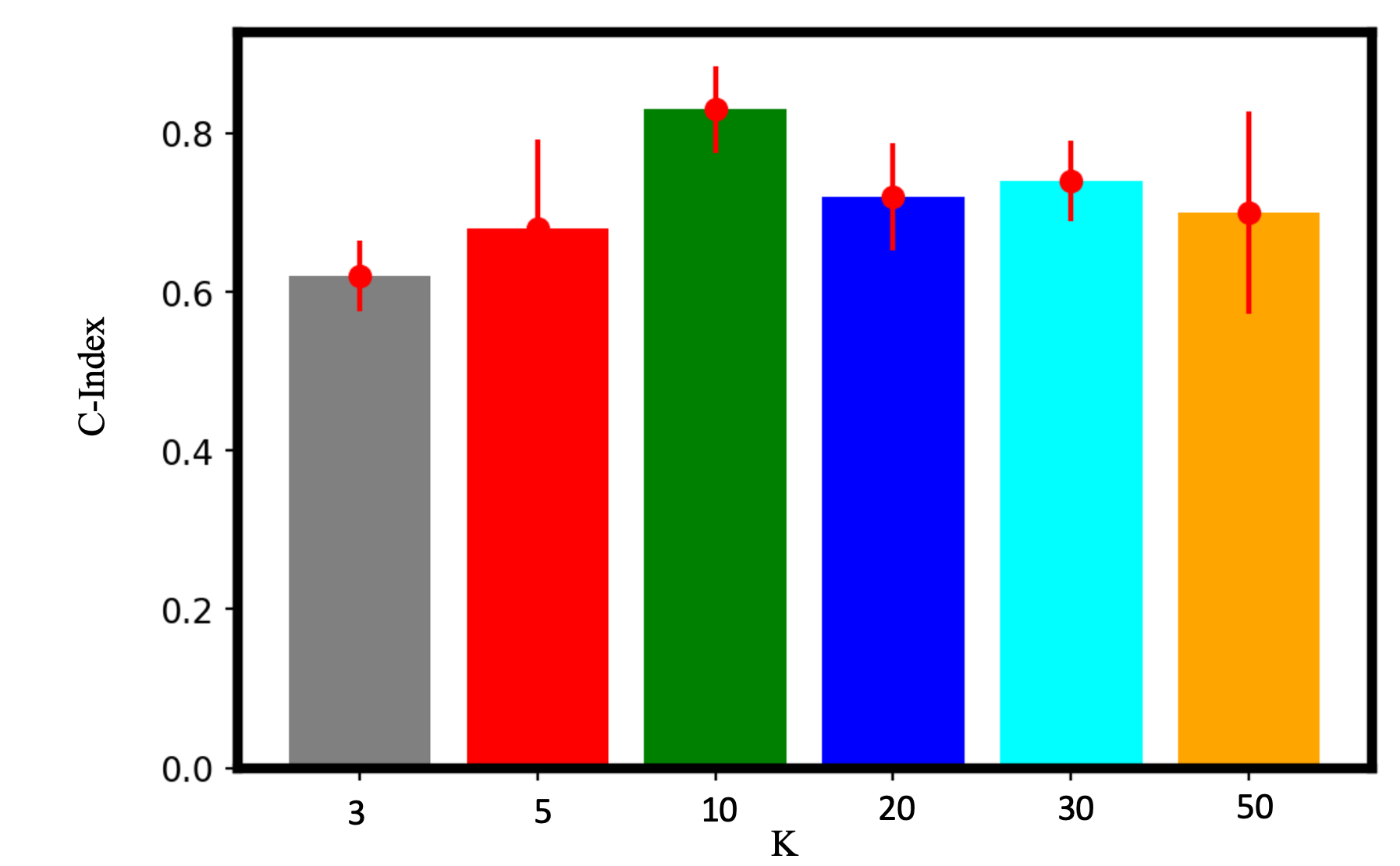
Figure 5: C-Index value under K = 3, 5, 10, 20, 30, 50 for TCGA-KIRP. The mean value and standard deviation for 5-fold cross-validation are plotted.

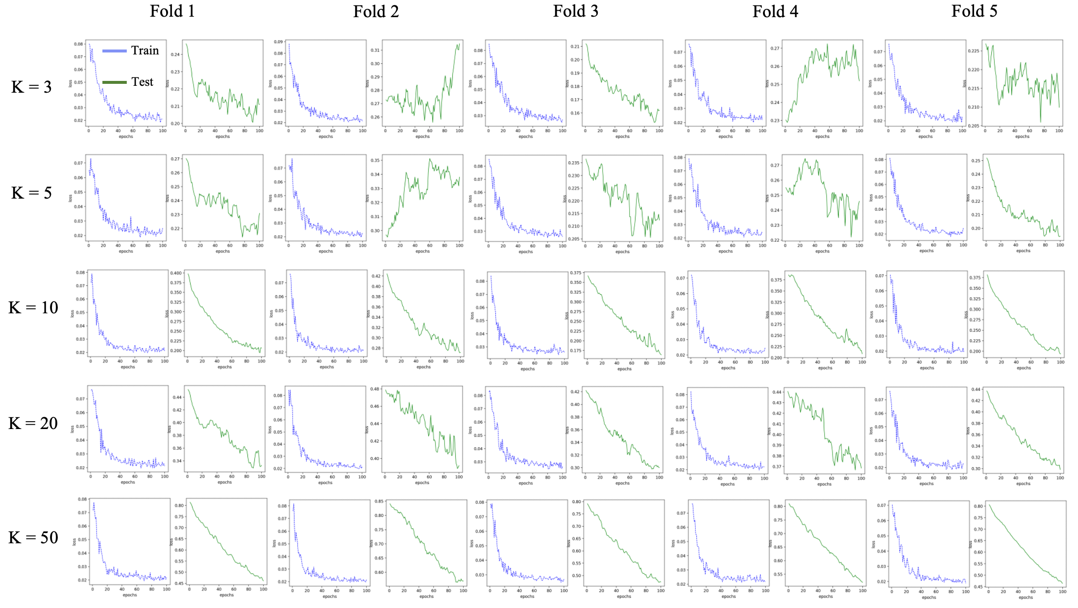
Figure 6: Train and test loss for TCGA-KIRP under K = 3, 5, 10, 20, 50 for 5-fold cross-validation.

C.3 Additional Results

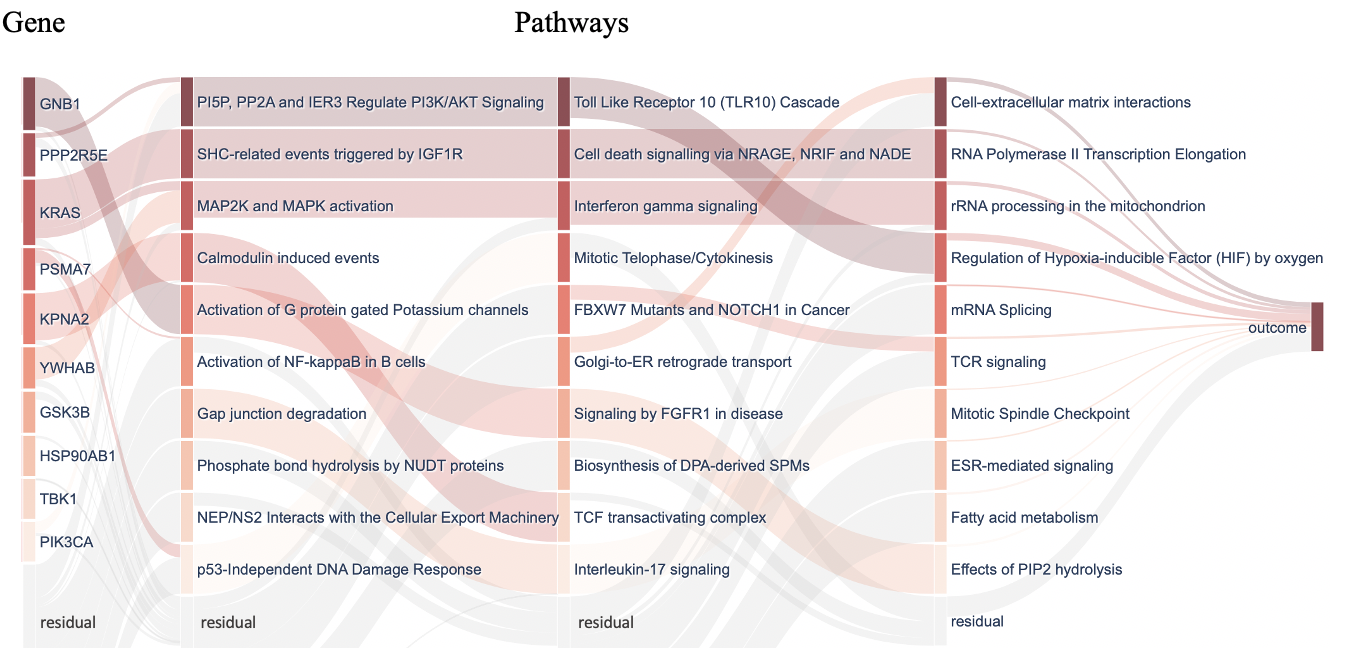
Figure 7: Inspecting and interpreting PONET on TCGA-BLCA. Sankey diagram visualization of the inner layers of PONET shows the estimated relative importance of different nodes in each layer. Nodes in the first layer represent genes; the next layers represent pathways; and the final layer represents the model outcome. Different layers are linked by weights. Nodes with darker colors are more important, while transparent nodes represent the residual importance of undisplayed nodes in each layer.

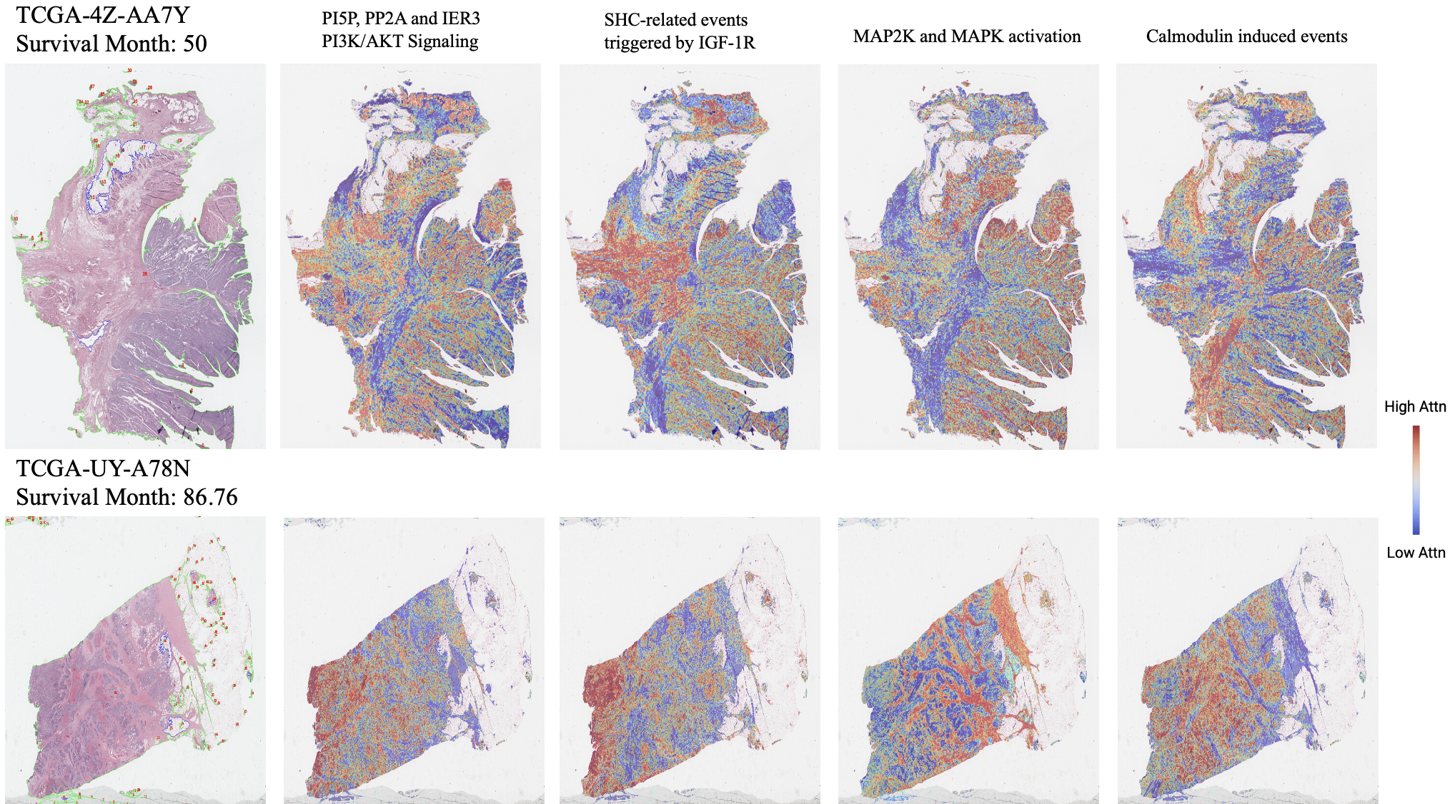
Figure 8: Co-attention visualization of top 4 ranked pathways in two cases of TCGA-BLCA.

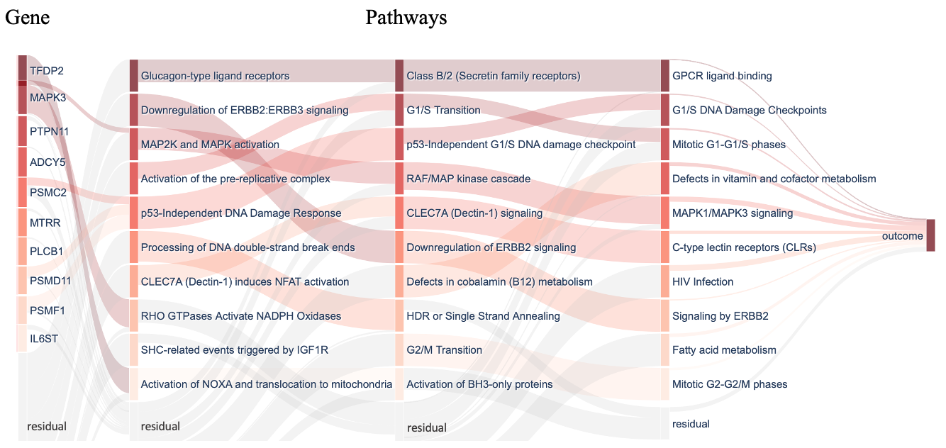
Figure 9: Inspecting and interpreting PONET on TCGA-KIRC. Sankey diagram visualization of the inner layers of PONET shows the estimated relative importance of different nodes in each layer. Nodes in the first layer represent genes; the next layers represent pathways; and the final layer represents the model outcome. Different layers are linked by weights. Nodes with darker colors are more important, while transparent nodes represent the residual importance of undisplayed nodes in each layer.

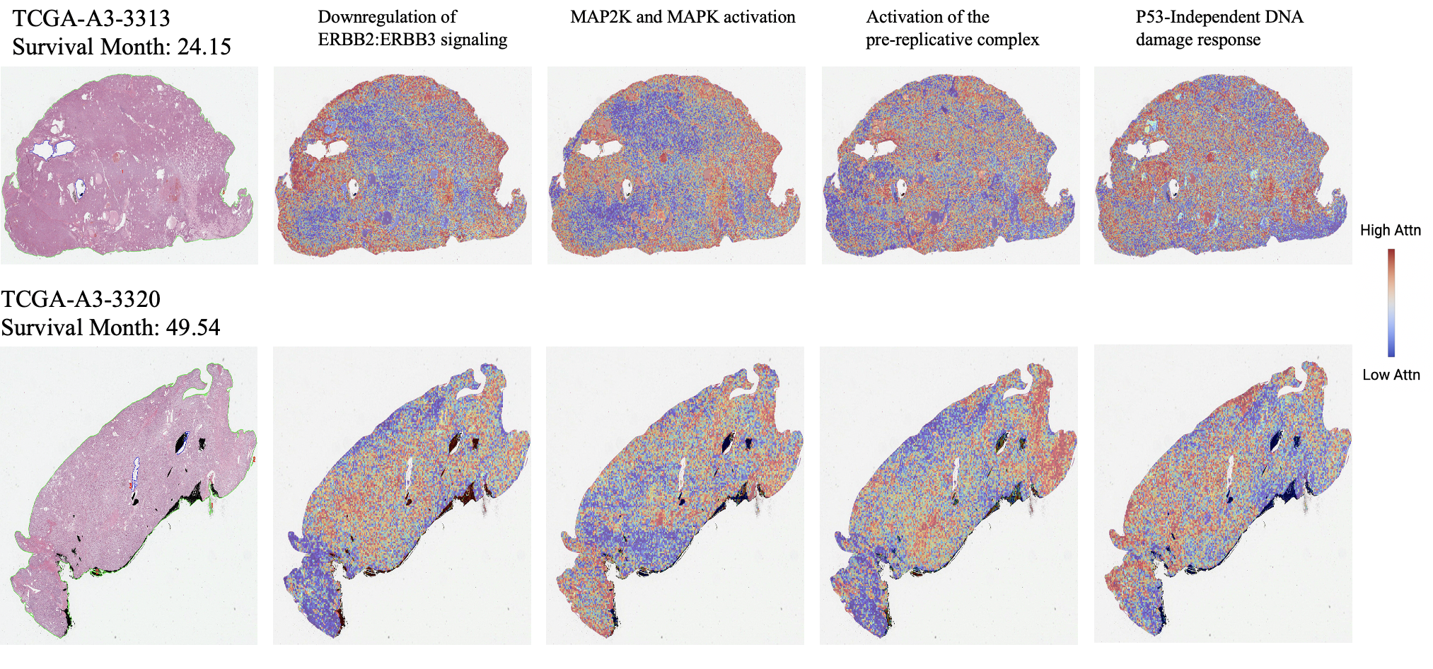
Figure 10: Co-attention visualization of top 4 ranked pathways in two cases of TCGA-KIRC.

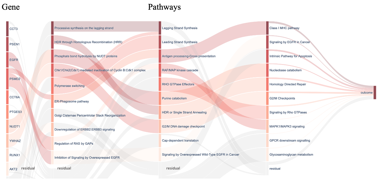
Figure 11: Inspecting and interpreting PONET on TCGA-LUAD. Sankey diagram visualization of the inner layers of PONET shows the estimated relative importance of different nodes in each layer. Nodes in the first layer represent genes; the next layers represent pathways; and the final layer represents the model outcome. Different layers are linked by weights. Nodes with darker colors are more important, while transparent nodes represent the residual importance of undisplayed nodes in each layer.

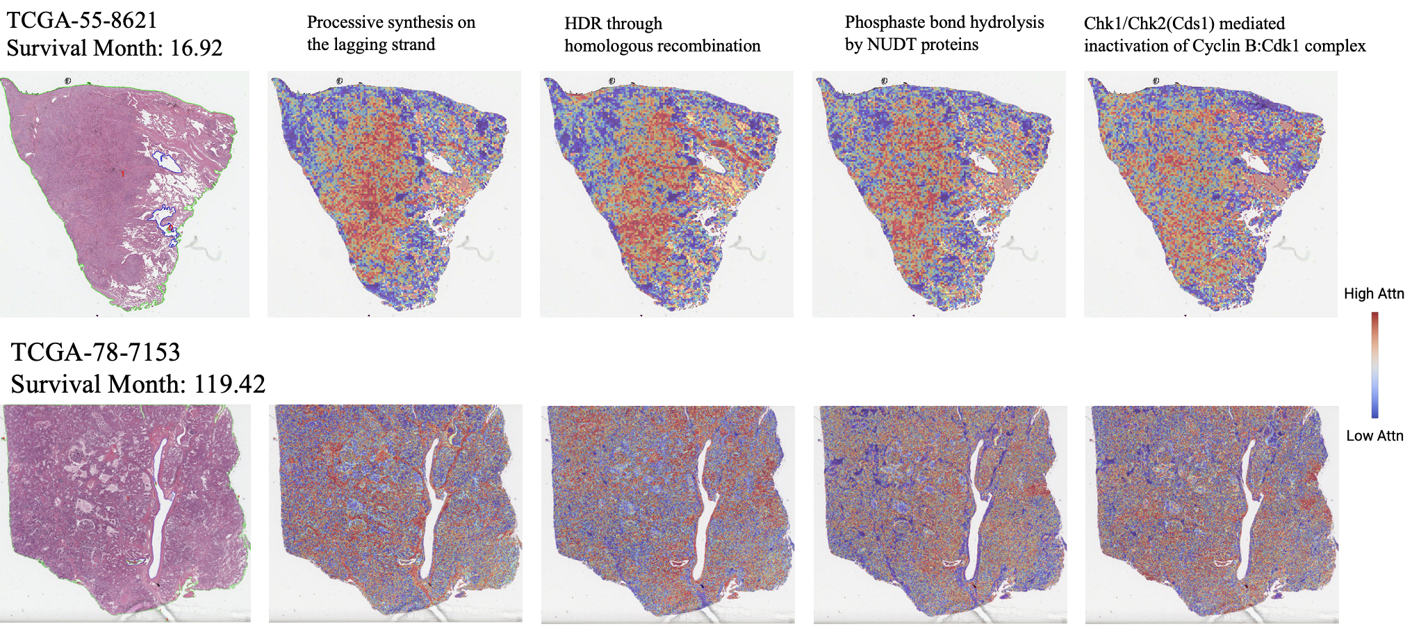
Figure 12: Co-attention visualization of top 4 ranked pathways in two cases of TCGA-LUAD.

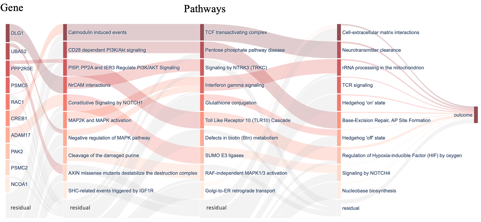
Figure 13: Inspecting and interpreting PONET on TCGA-LUSC. Sankey diagram visualization of the inner layers of PONET shows the estimated relative importance of different nodes in each layer. Nodes in the first layer represent genes; the next layers represent pathways; and the final layer represents the model outcome. Different layers are linked by weights. Nodes with darker colors are more important, while transparent nodes represent the residual importance of undisplayed nodes in each layer.

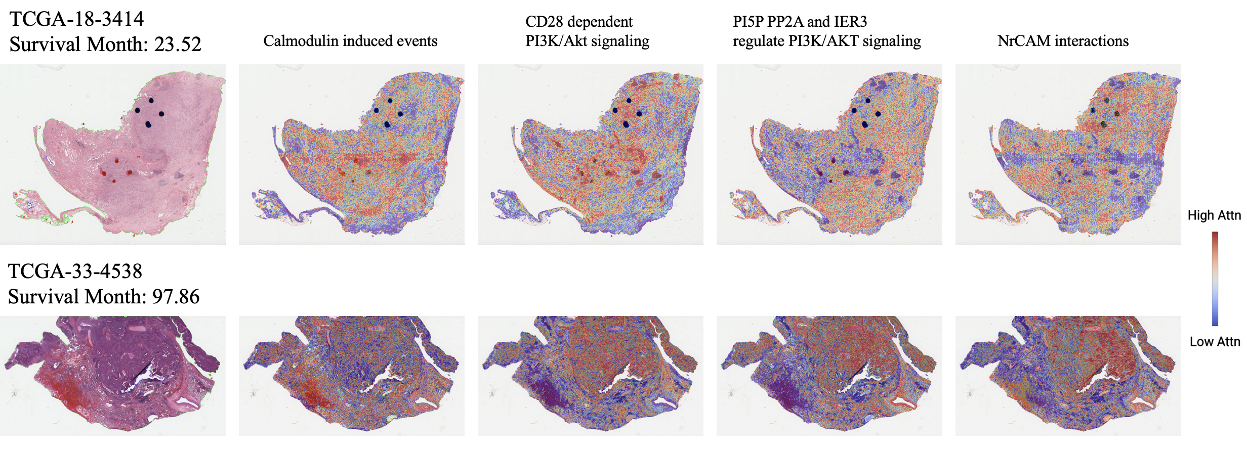
Figure 14: Co-attention visualization of top 4 ranked pathways in two cases of TCGA-LUSC.

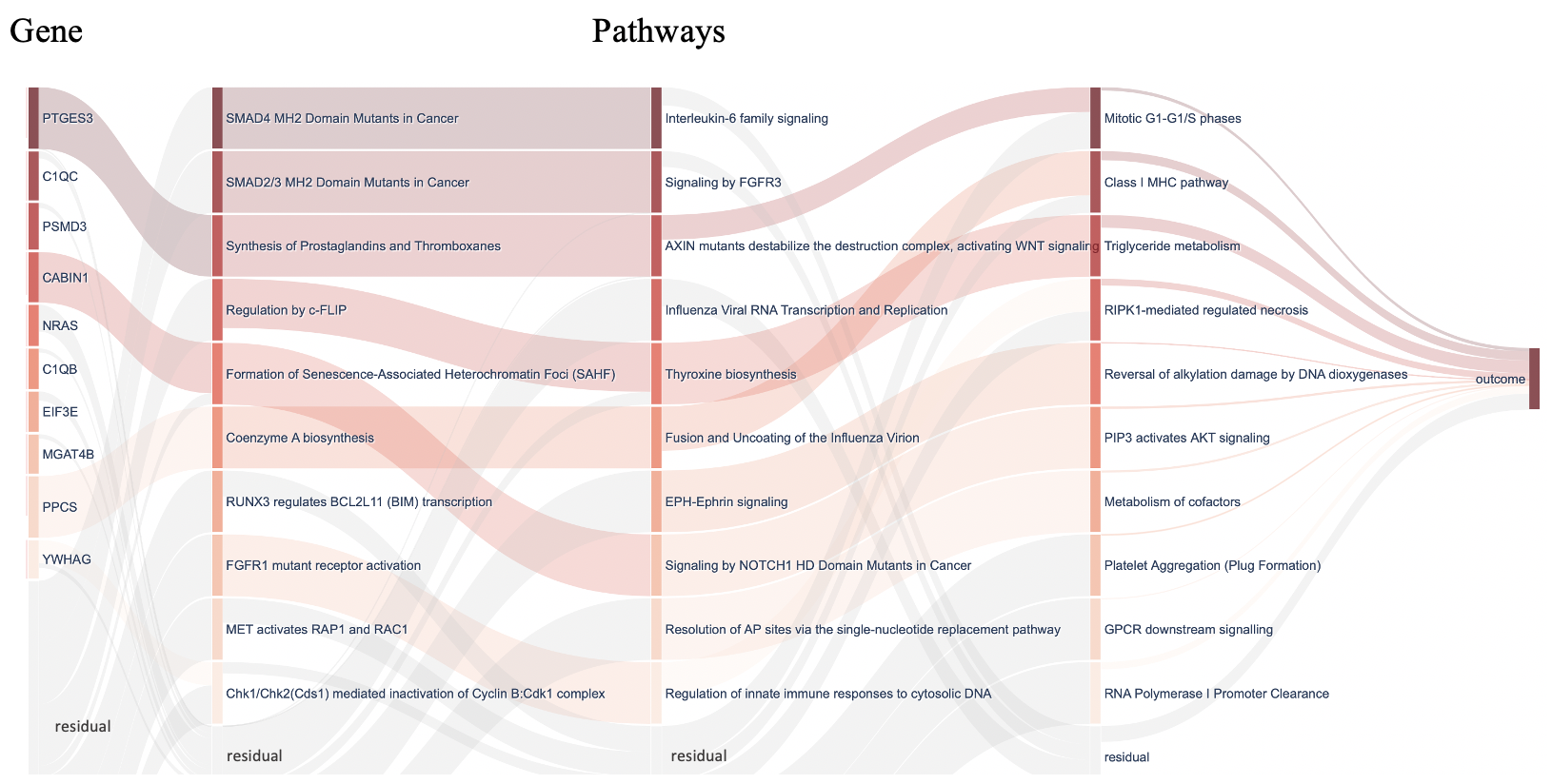
Figure 15: Inspecting and interpreting PONET on TCGA-PAAD. Sankey diagram visualization of the inner layers of PONET shows the estimated relative importance of different nodes in each layer. Nodes in the first layer represent genes; the next layers represent pathways; and the final layer represents the model outcome. Different layers are linked by weights. Nodes with darker colors are more important, while transparent nodes represent the residual importance of undisplayed nodes in each layer.

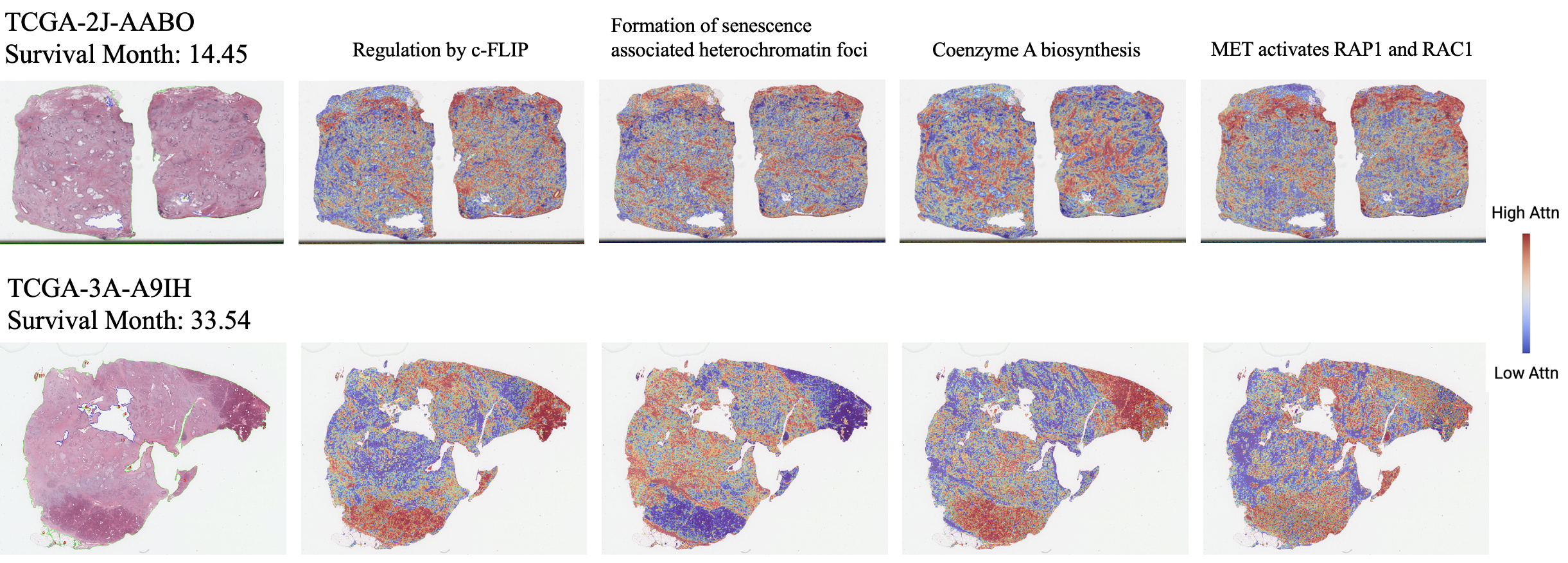
Figure 16: Co-attention visualization of top 4 ranked pathways in two cases of TCGA-PAAD.

References

- Al-Obaidy et al. (2020) Khaleel I Al-Obaidy, John N Eble, Mehdi Nassiri, Liang Cheng, Mohammad K Eldomery, Sean R Williamson, Wael A Sakr, Nilesh Gupta, Oudai Hassan, Muhammad T Idrees, et al. Recurrent kras mutations in papillary renal neoplasm with reverse polarity. Modern Pathology, 33(6):1157–1164, 2020.
- Chan (2014) John KC Chan. The wonderful colors of the hematoxylin-eosin stain in diagnostic surgical pathology. International Journal of Surgical Pathology, 22(1):12–32, 2014.
- Cheerla & Gevaert (2019) Anika Cheerla and Olivier Gevaert. Deep learning with multimodal representation for pancancer prognosis prediction. Bioinformatics, 35:i446–i454, 2019.
- Chen et al. (2021) Richard J Chen, Ming Y Lu, Wei-Hung Weng, Tiffany Y Chen, Drew FK Williamson, Trevor Manz, Maha Shady, and Faisal Mahmood. Multimodal co-attention transformer for survival prediction in gigapixel whole slide images. IEEE/CVF International Conference on Computer Vision, pp. 3995–4005, 2021.
- Chen et al. (2022a) Richard J Chen, Ming Y Lu, Jingwen Wang, Drew FK Williamson, Scott J Rodig, Neal I Lindeman, and Faisal Mahmood. Pathomic fusion: An integrated framework for fusing histopathology and genomic features for cancer diagnosis and prognosis. IEEE Transactions on Medical Imaging, 41(4):757–770, 2022a.
- Chen et al. (2022b) Richard J Chen, Ming Y Lu, Drew FK Williamson, Tiffany Y Chen, Jana Lipkova, Zahra Noor, Muhammad Shaban, Maha Shady, Mane Williams, Bumjin Joo, et al. Pan-cancer integrative histology-genomic analysis via interpretable multimodal deep learning. arXiv:2108.02278, 2022b.
- Cheng et al. (2017) Jun Cheng, Jie Zhang, Yatong Han, Xusheng Wang, Xiufen Ye, Yuebo Meng, Anil Parwani, Zhi Han, Qianjin Feng, and Kun Huang. Integrative analysis of histopathological images and genomic data predicts clear cell renal cell carcinoma prognosis. Cancer Research, 77(21):e91–e100, 2017.
- Cirillo et al. (2017) Elisa Cirillo, Laurence D Parnell, and Chris T Evelo. A review of pathway-based analysis tools that visualize genetic variants. Frontiers in Genetics, 8(174), 2017.
- Courtiol et al. (2019) Pierre Courtiol, Charles Maussion, Matahi Moarii, Elodie Pronier, Samuel Pilcer, Meriem Sefta, Pierre Manceron, Sylvain Toldo, Mikhail Zaslavskiy, Nolwenn Le Stang, et al. Deep learning-based classification of mesothelioma improves prediction of patient outcome. Nature Medicine, 25(10):1519–1525, 2019.
- Cox (1972) David R Cox. Regression models and life-tables. Journal of the Royal Statistical Society: Series B (Statistical Methodology), 34(2):187–202, 1972.
- Elmarakeby et al. (2021) Haitham A Elmarakeby, Justin Hwang, Rand Arafeh, Jett Crowdis, Sydney Gang, David Liu, Saud H AlDubayan, Keyan Salari, Steven Kregel, Camden Richter, et al. Biologically informed deep neural network for prostate cancer discovery. Nature, 598:348–352, 2021.
- Fabregat et al. (2020) Antonio Fabregat, Steven Jupe, Lisa Matthews, Konstantinos Sidiropoulos, Marc Gillespie, Phani Garapati, Robin Haw, Bijay Jassal, Florian Korninger, Bruce May, et al. The reactome pathway knowledgebase. Nucleic Acids Research, 48(D1):D498–D503, 2020.
- Grubb et al. (2022) Treg Grubb, Smruthi Maganti, John Michael Krill-Burger, Cameron Fraser, Laura Stransky, Tomas Radivoyevitch, Kristopher A. Sarosiek, Francisca Vazquez, William G. Kaelin Jr., and Abhishek A. Chakraborty. A mesenchymal tumor cell state confers increased dependency on the bcl-xl anti-apoptotic protein in kidney cancer. bioRxiv, 2022.
- Guo et al. (2022) Jing-Yi Guo, Zuo-qian Jing, Xue-jie Li, and Li-yuan Liu. Bioinformatic analysis identifying psmb 1/2/3/4/6/8/9/10 as prognostic indicators in clear cell renal cell carcinoma. International Journal of Medical Sciences, 19(5):796–812, 2022.
- Han et al. (2018) Zhezhu Han, Dongxu Kang, Yeonsoo Joo, Jihyun Lee, Geun-Hyeok Oh, Soojin Choi, Suwan Ko, Suyeon Je, Hye Jin Choi, and Jae J Song. Tgf-beta downregulation-induced cancer cell death is finely regulated by the sapk signaling cascade. Experimental and Molecular Medicine, 50(12):162, 2018.
- Hao et al. (2018) Jie Hao, Youngsoon Kim, Tae-Kyung Kim, and Mingon Kang. Pasnet: pathway-associated sparse deep neural network for prognosis prediction from high-throughput data. BMC Bioinformatics, 19:510, 2018.
- Harrell et al. (1982) Frank E Harrell, Robert M Califf, David B Pryor, Kerry L Lee, and Robert A Rosati. Evaluating the yield of medical tests. Journal of the American Medical Association, 247(18):2543–2546, 1982.
- Hekler et al. (2019) Achim Hekler, Jochen S Utikal, Alexander H Enk, Wiebke Solass, Max Schmitt, Joachim Klode, Dirk Schadendorf, Wiebke Sondermann, Cindy Franklin, Felix Bestvater, et al. Deep learning outperformed 11 pathologists in the classification of histopathological melanoma images. Europe Journal of Cancer, 118:91–6, 2019.
- Hou et al. (2016) Le Hou, Dimitris Samaras, Tahsin M Kurc, Yi Gao, James E Davis, and Joel H Saltz. Patch-based convolutional neural network for whole slide tissue image classification. In Proceedings of the IEEE/CVF Conference on Computer Vision and Pattern Recognition, pp. 2424–2433, 2016.
- Hou et al. (2020) Le Hou, Rajarsi Gupta, John S Van Arnam, Yuwei Zhang, Kaustubh Sivalenka, Dimitris Samaras, Tahsin M Kurc, and Joel H Saltz. Dataset of segmented nuclei in hematoxylin and eosin stained histopathology images of ten cancer types. Scientific Data, 7(1):185, 2020.
- Iizuka et al. (2020) Osamu Iizuka, Fahdi Kanavati, Kei Kato, Michael Rambeau, Koji Arihiro, and Masayuki Tsuneki. Deep learning models for histopathological classification of gastric and colonic epithelial tumours. Scientific Report, 10(1):1504, 2020.
- Ilse et al. (2018) Maximilian Ilse, Jakub Tomczak, and Max Welling. Attention-based deep multiple instance learning. In Proceedings of the 35th International Conference on Machine Learning, volume 80, pp. 2127–2136, 2018.
- Jin et al. (2014) Lv Jin, Xiao-Yu Zuo, Wei-Yang Su, Xiao-Lei Zhao, Man-Qiong Yuan, Li-Zhen Han, Xiang Zhao, Ye-Da Chen, and Shao-Qi Rao. Pathway-based analysis tools for complex diseases: A review. Genomics Proteomics Bioinformatics, 12(5):210–220, 2014.
- Kampman et al. (2018) Onno Kampman, Elham J Barezi, Dario Bertero, and Pascale Fung. Investigating audio, video, and text fusion methods for end-to-end automatic personality prediction. In Proceedings of the 56th Annual Meeting of the Association for Computational Linguistics (Volume 2: Short Papers), pp. 606–611, 2018.
- Katzman et al. (2018) Jared L. Katzman, Uri Shaham, Alexander Cloninger, Jonathan Bates, Tingting Jiang, and Yuval Kluger. Deepsurv: personalized treatment recommender system using a cox proportional hazards deep neural network. BMC Medical Research Methology, 18(24):187–202, 2018.
- Kim et al. (2017) Jin-Hwa Kim, Kyoung-Woon On, Woosang Lim, Jeonghee Kim, Jung-Woo Ha, and Byoung-Tak Zhang. Hadamard product for low-rank bilinear pooling. In Proceedings of International Conference on Learning Representations, pp. 1–14, 2017.
- Li et al. (2022) Ruiqing Li, Xingqi Wu, Ao Li, and Minghui Wang. Hfbsurv: hierarchical multimodal fusion with factorized bilinear models for cancer survival prediction. Bioinformatics, 38(9):2587–2594, 2022.
- Li et al. (2015) Yanming Li, Bin Nan, and Ji Zhu. Multivariate sparse group lasso for the multivariate multiple linear regression with an arbitrary group structure. Biometrics, 71(2):354–63, 2015.
- Lin et al. (2017) Shuheng Lin, Ana Negulescu, Sirisha Bulusu, Benjamin Gibert, Jean-Guy Delcros, Benjamin Ducarouge, Nicolas Rama, Nicolas Gadot, Isabelle Treilleux, Pierre Saintigny, et al. Non-canonical notch3 signalling limits tumour angiogenesis. Nature Communications, 8:16074, 2017.
- Liu et al. (2021) Zhun Liu, Ying Shen, Varun Bharadhwaj Lakshminarasimhan, Paul Pu Liang, Amir Zadeh, and Louis-Philippe Morency. Efficient low-rank multimodal fusion with modality-specific factors. In Proceedings of the 56th Annual Meeting of the Association for Computational Linguistics, pp. 2247–2256, 2021.
- Lu et al. (2021) Ming Y Lu, Drew FK Williamson, Tiffany Y Chen, Richard J Chen, Matteo Barbieri, and Faisal Mahmood. Data-efficient and weakly supervised computational pathology on whole-slide images. Nature Biomedical Engineering, 5:555–570, 2021.
- Mai et al. (2020) Sijie Mai, Haifeng Hu, and Songlong Xing. Modality to modality translation: An adversarial representation learning and graph fusion network for multimodal fusion. In Proceedings of the AAAI Conference on Artificial Intelligence, pp. 164–172, 2020.
- Mallavarapu et al. (2017) Tejaswini Mallavarapu, Youngsoon Kim, Jung Hun Oh, and Mingon Kang. R-pathcluster: Identifying cancer subtype of glioblastoma multiforme using pathway-based restricted boltzmann machine. In 2017 IEEE International Conference on Bioinformatics and Biomedicine, pp. 1183–8, 2017.
- Mobadersany et al. (2018) Pooya Mobadersany, Safoora Yousefi, Mohamed Amgad, David A Gutman, Jill S Barnholtz-Sloan, José E Velázquez Vega, Daniel J Brat, and Lee AD Cooper. Predicting cancer outcomes from histology and genomics using convolutional networks. Proceedings of the National Academy of Sciences, 115(13):E2970–E2979, 2018.
- Ning et al. (2020) Zhenyuan Ning, Weihao Pan, Yuting Chen, Qing Xiao, Xinsen Zhang, Jiaxiu Luo, Jian Wang, and Yu Zhang. Integrative analysis of cross-modal features for the prognosis prediction of clear cell renal cell carcinoma. Bioinformatics, 36(9):2888–2895, 2020.
- Nojavanasghari et al. (2016) Behnaz Nojavanasghari, Deepak Gopinath, Jayanth Koushik, Tadas Baltrušaitis, and Louis-Philippe Morency. Deep multimodal fusion for persuasiveness prediction. In Proceedings of the 18th ACM International Conference on Multimodal Interaction, pp. 284–288, 2016.
- Pan et al. (2017) Xipeng Pan, Lingqiao Li, Huihua Yang, Zhenbing Liu, Jinxin Yang, Lingling Zhao, and Yongxian Fan. Accurate segmentation of nuclei in pathological images via sparse reconstruction and deep convolutional networks. Neurocomputing, 15:88–99, 2017.
- Poria et al. (2016) Soujanya Poria, Iti Chaturvedi, Erik Cambria, and Amir Hussain. Convolutional mkl based multimodal emotion recognition and sentiment analysis. In Proceedings of International Conference on Data Mining, pp. 439–448, 2016.
- Shan et al. (2017) Guang Shan, Tian Tang, Huijun Qian, and Yue Xia. Expression of tiam1 and rac1 proteins in renal cell carcinoma and its clinical-pathological features. International Journal of Clinical and Experimental Pathology, 10(11):11114–11121, 2017.
- Subramanian et al. (2021) Vaishnavi Subramanian, Tanveer Syeda-Mahmood, and Minh N Do. Multimodal fusion using sparse cca for breast cancer survival prediction. In Proceedings of IEEE 18th International Symposium on Biomedical Imaging (ISBI), pp. 1429–1432, 2021.
- Sundararajan et al. (2017) Mukund Sundararajan, Ankur Taly, and Qiqi Yan. Axiomatic attribution for deep networks. In Proceedings of the 34th International Conference on Machine Learning, volume 70, pp. 3319–3328, 2017.
- Tenenbaum & Freeman (2000) Joshua B Tenenbaum and William T Freeman. Separating style and content with bilinear models. Neural Computation, 12(6):1247–1283, 2000.
- Wang et al. (2020) Chunyu Wang, Junling Guo, Ning Zhao, Yang Liu, Xiaoyan Liu, Guojun Liu, and Maozu Guo. A cancer survival prediction method based on graph convolutional network. IEEE Trans Nanobioscience, 19(1):117–126, 2020.
- Wang et al. (2021a) Xiyue Wang, Sen Yang, Jun Zhang, Minghui Wang, Jing Zhang, Junzhou Huang, Wei Yang, and Xiao Han. Transpath: Transformer-based self-supervised learning for histopathological image classification. In International Conference on Medical Image Computing and Computer-Assisted Intervention, pp. 186–195. Springer, 2021a.
- Wang et al. (2021b) Zhiqin Wang, Ruiqing Li, Minghui Wang, and Ao Li. Gpdbn: deep bilinear network integrating both genomic data and pathological images for breast cancer prognosis prediction. Bioinformatics, 27(18):2963–2970, 2021b.
- Wöllmer et al. (2013) Martin Wöllmer, Felix Weninger, Tobias Knaup, Björn Schuller, Congkai Sun, Kenji Sagae, and Louis-Philippe Morency. Youtube movie reviews: Sentiment analysis in an audio-visual context. IEEE Intelligent Systems, 28(3):46–53, 2013.
- Wulczyn et al. (2020) Ellery Wulczyn, David F Steiner, Zhaoyang Xu, Apaar Sadhwani, Hongwu Wang, Isabelle Flament-Auvigne, Craig H Mermel, Po-Hsuan Cameron Chen, Yun Liu, and Martin C Stumpe. Deep learning-based survival prediction for multiple cancer types using histopathology images. Plos One, 15(6):e0233678, 2020.
- Yang et al. (2017) Chun-ming Yang, Shan Ji, Yan Li, Li-ye Fu, Tao Jiang, and Fan-dong Meng. B-catenin promotes cell proliferation, migration, and invasion but induces apoptosis in renal cell carcinoma. OncoTargets and Therapy, 10:711–724, 2017.
- Yu et al. (2017) Zhou Yu, Jun Yu, Jianping Fan, and Dacheng Tao. Multi-modal factorized bilinear pooling with co-attention learning for visual question answering. In IEEE International Conference on Computer Vision, pp. 1839–1848, 2017.
- Zadeh et al. (2016) Amir Zadeh, Rowan Zellers, Eli Pincus, and Louis-Philippe Morency. Multimodal sentiment intensity analysis in videos: Facial gestures and verbal messages. IEEE Intelligent Systems, pp. 82–88, 2016.
- Zadeh et al. (2017) Amir Zadeh, Minghai Chen, Soujanya Poria, Erik Cambria, and Louis-Philippe Morency. Tensor fusion network for multimodal sentiment analysis. In Proceedings of the 2017 Conference on Empirical Methods in Natural Language Processing, pp. 1103–1114, 2017.
- Zadeh & Schmid (2020) Shekoufeh Gorgi Zadeh and Matthias Schmid. Bias in cross-entropy-based training of deep survival networks. IEEE Transactions on Pattern Analysis and Machine Intelligence, 43(9):3126–3137, 2020.
- Zhang et al. (2019) Qiang Zhang, Xiujuan Yin, Zhiwei Pan, Yingying Cao, Shaojie Han, Guojun Gao, Zhiqin Gao, Zhifang Pan, and Weiguo Feng. Identification of potential diagnostic and prognostic biomarkers for prostate cancer. Oncology Letters, 18(4):4237–4245, 2019.