Spatio-temporal determinantal point processes

Abstract

Determinantal point processes are models for regular spatial point patterns, with appealing probabilistic properties. We present their spatio-temporal counterparts and give examples of these models, based on spatio-temporal covariance functions which are separable and non-separable in space and time.

Keywords: Covariance function; point process; regularity; spatio-temporal; spectral density

1 Introduction

Spatio-temporal point processes are random countable subsets $X$ of $\mathbb{R}^{2}\times\mathbb{R}^{+}$, where a point $(u,t)\in X$ corresponds to an event $u\in\mathbb{R}^{2}$ occurring at time $t\in\mathbb{R}^{+}$. We assume that the points do not overlap, i.e. $(u_{1},t_{1})\neq(u_{2},t_{2})$. Examples of such events are the occurrence of epidemic diseases (such as corona or flu), sightings or births of a species, the occurrence of fires, earthquakes, tsunamis, or volcanic eruptions. We are interested here in spatio-temporal regular point processes, where neighbouring points in the process tend to repel each other.

In the context of spatial point processes, Gibbs point processes including Markov point processes and pairwise interaction point process models are generally used to model repulsiveness. Another class of regular spatial point process models are determinantal point processes (dpps), which have their origin in quantum physics. They were first identified as a class by Macchi (1975), who called them fermion processes because they reflect the distributions of fermion systems in thermal equilibrium that exhibit repulsive behaviour. dpps have been extensively studied in probability theory and have found applications in random matrix theory, quantum physics, wireless network modelling, Monte Carlo integration, and machine learning (see e.g. Lavancier et al., 2015). Recently, Lavancier et al. (2015) studied the statistical properties of dpps.

Some regular spatial point process models have already their spatio-temporal counterparts, but likelihood-based inference or simulation of these models is usually complicated and time-consuming. To circumvent these challenges, our objective here is to introduce the spatio-temporal determinantal point processes (stdpps) and study their properties, which is an open problem according to Lavancier et al. (2015, pages 875-876). We present the basic properties of these processes and give examples of them based on separable and non-separable spatio-temporal covariance functions. We derive the key summary characteristics for these examples that can be used, for example, for model fitting and evaluation.

2 Basic concepts and statistical properties

Assume that $X$ is a spatio-temporal point process with $n$th-order product density $\rho^{(n)}$, $n\geq 1$ which describes the frequency of possible configurations of $n$ points. Suppose that $B_{1},\ldots,B_{n}$ are pairwise disjoint cylindrical regions having infinitesimal volumes $dV_{1},\ldots,dV_{n}$ and containing the points $((u_{1},t_{1}),\dots,(u_{n},t_{n}))$, respectively. Then, $\rho^{(n)}\big{(}(u_{1},t_{1}),\ldots,(u_{n},t_{n})\big{)}dV_{1},\ldots dV_{n}$ is the probability that $X$ has a point in each of $B_{1},\ldots,B_{n}$.

Definition 1.

Let $C$ be a kernel function from $(\mathbb{R}^{2}\times\mathbb{R}^{+})\times(\mathbb{R}^{2}\times\mathbb{R}^{+})$ to $\mathbb{R}$. We say that a spatio-temporal point process $X$ is a determinantal point process with kernel $C$ and write $X\sim\textsc{stdpp}{}(C)$, if its $n$th-order product density function is given by

$$\rho^{(n)}((u_{1},t_{1}),\ldots,(u_{n},t_{n}))=\det\{C((u_{i},t_{i}),(u_{j},t_{j}))\}_{1\leq i,j\leq n},$$

for $(u_{i},t_{i})\in(\mathbb{R}^{2}\times\mathbb{R}^{+})$ and $n=1,2,\ldots$, where $\{C((u_{i},t_{i}),(u_{j},t_{j})\}_{1\leq i,j\leq n}$ is the $n\times n$ matrix with $C((u_{i},t_{i}),(u_{j},t_{j}))$ as its $(i,j)$-th entry and $\det\{A\}$ is the determinant of the matrix $A$.

The point process $X$ is well-defined if, for each $n$, $\rho^{(n)}((u_{1},t_{1}),\cdots,(u_{n},t_{n}))\geq 0$ for all $\{(u_{i},t_{i})\}_{i=1}^{n}$. This implies that, in Definition 1, $\mathbf{C}=\{C((u_{i},t_{i}),(u_{j},t_{j})\}_{1\leq i,j\leq n}$ should be a non-negative definite matrix. Then all eigenvalues of the matrix $\mathbf{C}$ are non-negative and thus its determinant is also non-negative (this follows from the fact that the determinant of a matrix is equal to the product of its eigenvalues) (Radhakrishna Rao and Bhaskara Rao, 1998). Therefore, covariance functions are possible choices for the kernel $C$. Denoting the eigenvalues of $\mathbf{C}$ by $\lambda_{l}$ $(l=1,2,\ldots)$, another condition for the existence of stdpp($C$) is that $\lambda_{l}\leq 1$ $(l=1,2,\ldots)$. This is a straightforward extension from the spatial setting, see details in Lavancier et al. (2015) and the references therein. The Poisson process with intensity $\rho(u,s)$ results as a special case of stdpp($C$) with setting $C((u,s),(u,s))=\rho(u,s)$ and $C((u,s),(v,t))=0\,\,\mbox{if}\,\,u\neq v\,\mbox{or}\,s\neq t$.

By Definition 1, the moment characteristics of arbitrary order $n$ $(n\geq 1)$ can be easily attained for stdpps, e.g. the intensity function is given by $\rho(u,t)=C((u,t),(u,t))$ and the second-order product density is given by

$$\rho^{(2)}((u_{1},t_{1}),(u_{2},t_{2})) =C\left((u_{1},t_{1}),(u_{1},t_{1})\right)C((u_{2},t_{2}),(u_{2},t_{2}))$$

$$-C((u_{1},t_{1}),(u_{2},t_{2}))C((u_{1},t_{1}),(u_{2},t_{2})).$$

In what follows, we assume that the kernel function is of the form

$$C((u_{1},t_{1}),(u_{2},t_{2}))=\sqrt{\rho(u_{1},t_{1})}R\Big{(}(u_{1},t_{1})/\alpha_{s},(u_{2},t_{2})/\alpha_{t}\Big{)}\sqrt{\rho(u_{2},t_{2})},$$

where $\rho$ plays the role of the intensity function of the process, $\alpha_{s}>0$ and $\alpha_{t}>0$ are the spatial and temporal correlation parameters respectively, and $R(\cdot)$ is the correlation function correspondent to $C$. Then, the (inhomogeneous space-time) pair correlation function is given by

$$g((u_{1},t_{1}),(u_{2},t_{2})) =\frac{\rho^{(2)}((u_{1},t_{1}),(u_{2},t_{2}))}{\rho(u_{1},t_{1})\rho(u_{2},t_{2})}$$ (1)

$$=1-\Big{\lvert}R\Big{(}(u_{1},t_{1})/\alpha_{s},(u_{2},t_{2})/\alpha_{t}\Big{)}\Big{\rvert}^{2}\leq 1.$$ (2)

Since $g\leq 1$, the points of $X$ repel each other, which is a characteristic of regular point patterns.

In general, a stdpp is called second-order intensity reweighted stationary (soirs) if its space-time pair correlation function is a function of the spatial difference $u=u_{2}-u_{1}$ and the temporal difference $t=t_{2}-t_{1}$ (see, e.g. Ghorbani, 2013, and the references therein). Thus, a stdpp with kernel function $C$ is soirs if the correlation function $R$ is a function of $u$ and $r$ only, i.e. if $R$ takes the form $R((u_{1},t_{1}),(u_{2},t_{2}))=R_{0}(u,t)$ for some function $R_{0}$. For a soirs stdpp(C), $R_{0}(0,0)=1$, and hence $\rho(u,t)=C(0,0)$. If in addition, the correlation function $R_{0}$ is invariant under rotation, i.e. isotropic, then it as well as the pair correlation function (1) depend only on the spatial distance $\lVert u\rVert$ and the temporal lag $\lvert t\rvert$. The pair correlation function is then given by

$$g(u,t)=1-\Big{\lvert}R_{0}(\|u\|/\alpha_{s},\lvert t\rvert/\alpha_{t})\Big{\rvert}^{2}.$$ (3)

Further, the space-time $K$-function (see e.g. Gabriel and Diggle, 2009; Møller and Ghorbani, 2012) is given by

$$K(u,t) =2\pi\int_{0}^{t}\int_{0}^{u}g(u^{\prime},t^{\prime})u^{\prime}\mathrm{d}u^{\prime}\mathrm{d}t^{\prime}$$ (4)

$$=\pi u^{2}t-\int_{0}^{u}\int_{0}^{t}\lvert R_{0}(\|u^{\prime}\|/\alpha_{s},\lvert t^{\prime}\rvert/\alpha_{t})\rvert^{2}u^{\prime}\mathrm{d}u^{\prime}\mathrm{d}t^{\prime}.$$ (5)

If the intensity $\rho$ is constant, i.e. $\rho(u,t)=\rho$, then the process is stationary and the corresponding stationary space-time $g$- and $K$-functions obtain the same formulas (3) and (4) under the isotropy assumption.

3 Examples of spatio-temporal determinantal point processes

Section 3.1 recalls the relationship between the covariance function and its spectral density. Then, in Sections 3.2 and 3.3, the Fourier transform of positive finite measures, i.e. spectral measures, are used to construct stationary spatio-temporal covariance functions, and characteristics of stdpps with these kernels are derived.

3.1 The covariance function and its spectral density

The covariance function of a stationary process can be represented as a Fourier transform of a positive finite measure. According to the Wiener-Khintchine theorem (see, e.g. Rasmussen and Williams, 2006), if the spectral density function $\varphi(\cdot,\cdot)$ exists, the covariance function $C(\cdot,\cdot)$ and the spectral density $\varphi(\cdot,\cdot)$ are Fourier duals of each other given by

$$C(u,t) =\int_{\mathbb{R}^{d+1}}e^{2\pi i(\omega^{T}u+\tau t)}\varphi(\omega,\tau)\mathrm{d}\omega\mathrm{d}\tau,$$ (6)

$$\varphi(\omega,\tau) =\int_{\mathbb{R}^{d+1}}e^{-2\pi i(\omega^{T}u+\tau t)}C(u,t)\mathrm{d}u\mathrm{d}t,$$ (7)

where $T$ stands for transpose, $\omega$ is the $d$-dimensional spatial component and $\tau$ is the temporal component.

A straightforward generalization of Proposition 3.1 in Lavancier et al. (2015) to the spatio-temporal setting, under continuity and stationarity of $C(u,t)$, when $C(u,t)\in\mathbb{L}^{2}(\mathbb{R}^{d}\times\mathbb{R}^{+})$, implies that a stdpp with kernel $C$ exists if the corresponding spectral density satisfies

$$\varphi(\omega,\tau)\leq 1.$$ (8)

3.2 Separable spatio-temporal covariance functions

A class of separable spatio-temporal covariance functions is usually given by

$$C_{0}(u,t)\propto C_{0}^{s}(u)C_{0}^{t}(t),$$ (9)

which is valid (i.e. a positive definite function) if both the spatial covariance function, $C_{0}^{s}(u)$, and the temporal covariance function, $C_{0}^{t}(t)$, are valid covariance functions. For a separable class of covariance functions, the spectral density $\varphi(\omega,\tau)$ has also a separable form, namely

$$\varphi(\omega,\tau)\propto\Big{[}\int_{\mathbb{R}^{d}}e^{-2\pi i\omega^{T}u}C_{0}^{s}(u)\mathrm{d}u\Big{]}\times\Big{[}\int_{\mathbb{R}}e^{-2\pi i\tau t}C_{0}^{t}(t)\mathrm{d}t\Big{]}=\varphi_{0}^{s}(\omega)\varphi_{0}^{t}(\tau),$$

where $\varphi_{0}^{s}(\omega)$ and $\varphi_{0}^{t}(\tau)$ are the spatial and temporal spectral densities, respectively. According to (8), the condition $\varphi_{0}^{s}(\omega)\varphi_{0}^{t}(\tau)<1$ must be satisfied for a stdpp with kernel (9) to exist. Further, for this class, the pair correlation function takes the following simple form

$$g(u,t)=1-\lvert R_{0}^{s}(\|u\|/\alpha_{s})\rvert^{2}\lvert R_{0}^{t}(\lvert t\rvert/\alpha_{t})\rvert^{2},$$

where $R_{0}^{s}$ and $R_{0}^{t}$ are the correlation functions in space and time corresponding to $C_{0}^{s}$ and $C_{0}^{t}$, respectively. Therefore, by (4) the corresponding $K$-function is given by

$$K(u,t)=\pi u^{2}t-\int_{0}^{u}u^{\prime}\lvert R_{0}^{s}(u^{\prime}/\alpha_{s})\rvert^{2}\mathrm{d}u^{\prime}\int_{0}^{t}\lvert R_{0}^{t}(t^{\prime}/\alpha_{t})\rvert^{2}\mathrm{d}t^{\prime}.$$

There are a large number of classes of valid spatial and valid temporal covariance functions in the literature, for example the Matérn, power exponential and Gaussian classes, to name a few (see, e.g. Cressie and Wikle, 2011). As an example, we consider the Gaussian covariance function $C_{0}^{s}(u)=\sqrt{\rho}\sigma^{2}_{s}\exp(-\|u\|^{2}/\alpha_{s})$, $u\in\mathbb{R}^{2}$, with spectral density $\varphi_{0}^{s}(\omega)=\sqrt{\rho}\pi\sigma^{2}_{s}\alpha_{s}^{2}\exp(-\pi^{2}\alpha_{s}^{2}\|\omega\|^{2})$, and the exponential covariance function $C_{0}^{t}(t)=\sqrt{\rho}\sigma^{2}_{t}\exp(-\lvert t\rvert/\alpha_{t})$, $t\in\mathbb{R}^{+},$ with spectral density $\varphi_{0}^{t}(\tau)=(2\sqrt{\rho}\sigma^{2}_{t}\alpha_{t})/(1+4\pi^{2}\alpha_{t}^{2}\lvert\tau\rvert^{2})$. Here $\sigma^{2}_{s}$ and $\sigma^{2}_{t}$ are the variance parameters of the spatial and time components, respectively, and $\alpha_{s}>0$ and $\alpha_{t}>0$ are the corresponding range parameters. A stationary stdpp with intensity $\rho$ and the separable covariance function (9) with these components, i.e

$$C_{0}(u,t)=\rho\sigma^{2}_{s}\sigma^{2}_{t}\exp\Big{(}-\frac{\|u\|^{2}}{\alpha_{s}}-\frac{\lvert t\rvert}{\alpha_{t}}\Big{)}$$ (10)

will exist if

$$\varphi_{sep}(\omega,\tau)=\frac{2\pi\rho\alpha_{s}^{2}\alpha_{t}\sigma^{2}_{s}\sigma^{2}_{t}}{(1+4\pi^{2}\alpha_{t}^{2}\tau^{2})}\exp{\left(-\pi^{2}\alpha_{s}^{2}\|\omega\|^{2}\right)}<1.$$

Since the maximum of the spectral density occurs at $(0,0)$, so a stdpp($C_{0}$) exists if $\varphi_{sep}(0,0)<1$, which implies that $\rho<(2\pi\alpha_{s}^{2}\alpha_{t}\sigma^{2}_{s}\sigma^{2}_{t})^{-1}$, and hence the maximal intensity is $\rho_{\max}=(2\pi\alpha_{s}^{2}\alpha_{t}\sigma^{2}_{s}\sigma^{2}_{t})^{-1}.$ For this process the pair correlation function is simply given by

$$g(u,t)=1-\exp\Big{(}-\frac{2\|u\|^{2}}{\alpha_{s}}-\frac{2\lvert t\rvert}{\alpha_{t}}\Big{)}.$$ (11)

The corresponding $K$-function also has a closed-form expression, which is given in A.

Figure 1 (top row) shows that the values of the pair correlation function (11) decrease by the increase of the spatial range $\alpha_{s}$ and the temporal delay $\alpha_{t}$. Thus, these parameters determine the degree of repulsion for the above separable model.

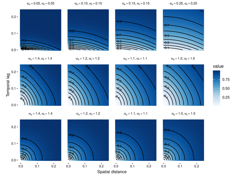
Figure 1: Theoretical pair correlation functions (11) (top row), (15) (middle row) and (18) (bottom row) for different values of the parameters given on top of the plots.

3.3 Non-separable spatio-temporal covariance function

Following Fuentes et al. (2007), we consider the spatio-temporal spectral density

$$\varphi_{\epsilon}(\omega,\tau)=\gamma(\alpha_{s}^{2}\alpha_{t}^{2}+\alpha_{t}^{2}\lvert\omega\rvert^{2}+\alpha_{s}^{2}\tau^{2}+\epsilon\lvert\omega\rvert^{2}\tau^{2})^{-\nu},$$ (12)

which is an extension of the commonly used Matérn spectral density (Cressie and Wikle, 2011). Here, the non-negative parameter $\alpha_{s}^{-1}$ (spatial range) explains the rate of decay of the spatial correlation, the non-negative parameter $\alpha_{t}^{-1}$ (temporal delay) explains the rate of decay for the temporal correlation. Further, $\gamma>0$ is a scale parameter. The parameter $\nu$ measures the degree of smoothness of the process and it should be larger than $(d+1)/2$ to have a well-defined spectral density. The parameter $\epsilon$ controls the interaction between the spatial and temporal components. For $0\leq\epsilon<1$ the spectral density is non-separable while it is separable when $\epsilon=1$. The maximum of the spectral density is $\gamma(\alpha_{s}^{2}\alpha_{t}^{2})^{-\nu}$ and accordingly a stdpp with spectral density (12) exists if $\gamma<(\alpha_{s}^{2}\alpha_{t}^{2})^{\nu}$.

In the separable case, i.e. when $\epsilon=1$, the spectral density is given by

$$\varphi_{\epsilon=1}(\omega,\tau)=\gamma(\alpha_{s}^{2}+\|\omega\|^{2})^{-\nu}(\alpha_{t}^{2}+\tau^{2})^{-\nu}=\varphi_{0}^{s}(\omega)\varphi_{0}^{t}(\tau).$$ (13)

In this case, $\varphi_{0}^{s}(\omega)$ and $\varphi_{0}^{t}(\tau)$ are Matérn-type spectral densities in space and time, respectively. Consequently, the corresponding separable spatio-temporal covariance function, combining (6), and (13) and using the equations 6.726.4 and 8.432.5 in Gradshteyn and Ryzhik (2007) and setting $d=2$, is given by

$$C_{0}(u,t) =\frac{4\gamma\pi\sqrt{\pi}}{2^{2\nu-1/2}(\Gamma(\nu))^{2}}\Big{(}\frac{2\pi\lvert t\rvert}{\alpha_{t}}\Big{)}^{\nu-1/2}\Big{(}\frac{2\pi\|u\|}{\alpha_{s}}\Big{)}^{\nu-1}$$

$$\times\mathcal{K}_{\nu-\frac{1}{2}}\Big{(}2\pi\alpha_{t}\lvert t\rvert\Big{)}\mathcal{K}_{\nu-1}\Big{(}2\pi\alpha_{s}\|u\|\Big{)},$$

where $\mathcal{K}_{\nu}(\cdot)$ is the modified Bessel function of the second kind of order $\nu$. $C_{0}(u,t)$ is proportional to the product of Matérn covariance functions in space and time. Using the special cases, $\mathcal{K}_{\frac{1}{2}}(r)=e^{-r}(2r/\pi)^{-1/2}$ and $\mathcal{K}_{\frac{3}{2}}(r)=e^{-r}(1+r^{-1})(2r/\pi)^{-1/2}$ (Abramowitz and Stegun, 1992), the above covariance function for $\nu=2$ can be presented as

$$C_{0}(u,t)=\frac{\gamma\pi^{2}}{4\alpha_{s}^{2}\alpha_{t}^{3}}(2\pi\alpha_{t}\lvert t\rvert+1)\exp(-2\pi\alpha_{t}\lvert t\rvert)(2\pi\alpha_{s}\|u\|)\mathcal{K}_{1}(2\pi\alpha_{s}\|u\|).$$ (14)

For this case, considering the fact that $\lim_{x\rightarrow 0}x\mathcal{K}_{1}(x)=1$ (Yang and Chu, 2017), the intensity of the process is $\rho=C_{0}(0,0)=(\gamma\pi^{2})/(4\alpha_{s}^{2}\alpha_{t}^{3})$. Hence, taking into account that $\gamma<\alpha_{s}^{4}\alpha_{t}^{4}$, a stdpp with kernel (14) exists if $4\rho\leq\pi^{2}\alpha_{s}^{2}\alpha_{t}$. For this separable case with $\epsilon=1$, considering (3), the pair correlation function is

$$g(u,t)=1-(2\pi\alpha_{t}\lvert t\rvert+1)^{2}\exp(-4\pi\alpha_{t}\lvert t\rvert)\Big{[}(2\pi\alpha_{s}\|u\|)\mathcal{K}_{1}(2\pi\alpha_{s}\|u\|)\Big{]}^{2}.$$ (15)

For $\epsilon\in(0,1)$ the spatio-temporal covariance function corresponding to (12) should be computed numerically as there is no exact closed-form expression. For the case $\epsilon=0$, the stationary non-separable spatial-temporal spectral density is given by

$$\varphi_{\epsilon=0}(\omega,\tau)=\gamma(\alpha_{s}^{2}\alpha_{t}^{2}+\alpha_{t}^{2}\lvert\omega\rvert^{2}+\alpha_{s}^{2}\tau^{2})^{-\nu}.$$ (16)

Combining (6) and (16), and using the equations 6.726.4 and 8.432.5 in Gradshteyn and Ryzhik (2007), the covariance function when $\epsilon=0$ is

$$C_{0}(u,t) =\frac{\gamma\pi^{\frac{d+1}{2}}}{2^{\nu-\frac{d+1}{2}}\Gamma(\nu)\alpha_{s}^{(2\nu-d)}\alpha_{t}^{(2\nu-1)}}\left\{2\pi\alpha_{s}\Big{(}(\frac{\alpha_{t}}{\alpha_{s}}t)^{2}+\|u\|^{2}\Big{)}^{1/2}\right\}^{\nu-\frac{d+1}{2}}$$

$$\times\mathcal{K}_{\nu-\frac{d+1}{2}}\left(2\pi\alpha_{s}\Big{(}(\frac{\alpha_{t}}{\alpha_{s}}t)^{2}+\|u\|^{2}\Big{)}^{1/2}\right).$$

According to (8), for $d=2$ and $\nu=2$, there exists a stdpp with kernel

$$C_{0}(u,t)=\frac{\gamma\pi^{2}}{2\alpha_{s}^{2}\alpha_{t}^{3}}\exp\left(-2\pi\Big{(}\alpha_{t}^{2}\lvert t\rvert^{2}+\alpha_{s}^{2}\|u\|^{2}\Big{)}^{1/2}\right)$$ (17)

if and only if $\gamma<\alpha_{s}^{4}\alpha_{t}^{4}$. Further, it holds that $\rho=C_{0}(0,0)=(\gamma\pi^{2})/(2\alpha_{s}^{2}\alpha_{t}^{3})$ for the covariance functions (17). Thus, under the condition $\gamma<\alpha_{s}^{4}\alpha_{t}^{4}$, it holds that $2\rho\leq\pi^{2}\alpha_{s}^{2}\alpha_{t}$. Therefore, for a stdpp with the above covariance function, the intensity should be at most $\rho_{max}=\pi^{2}\alpha_{s}^{2}\alpha_{t}/2$. Further, for this process the pair correlation function is simply given by

$$g(u,t)=1-\exp\left(-4\pi\Big{(}\alpha_{t}^{2}\lvert t\rvert^{2}+\alpha_{s}^{2}\|u\|^{2}\Big{)}^{1/2}\right).$$ (18)

The expression for the corresponding $K$-function can be found in A.

Figure 1 (middle and bottom rows) shows that the values of the theoretical pair correlations (15) and (18) decrease as $\alpha_{s}^{-1}$ and $\alpha_{t}^{-1}$ increase. Thus, for these models, the parameters $\alpha_{s}^{-1}$ and $\alpha_{t}^{-1}$ play the role of spatial range and time delay that determine the degree of repulsion. Moreover, for fixed range parameters, the separable covariance model with (15) leads to smaller values of the pair correlation function and thus more repulsive patterns than the non-separable model with (18). While the separable covariance function controls to repulsiveness of points in space and time separately, in the non-separable case the points repel each other in the 3D space. This leads to the different small scale interactions.

4 Discussion and conclusion

The different forms of covariance functions presented here allow for stdpps with different types of repulsion. While empirical experiments in the spatio-temporal setting are to be conducted in future work, model fitting for dpps is available through the maximum likelihood or minimum contrast methods (Lavancier et al., 2015) based on the summary functions such as the pair correlation function presented here for the given examples, and for model assessment, e.g. the global envelope test (Myllymäki et al., 2017) can be employed.

Appendix A $K$-functions of the proposed models

Here we give the $K$-functions for two covariance models discussed in Section 3. The $K$-function of the model with the separable covariance function model (10), and correspondent to the pair correlation function (11), has the following closed-form expression:

$$K(u,t) =\pi u^{2}t-\int_{0}^{u}\int_{0}^{t}\exp\Big{(}\frac{-2u^{\prime 2}}{\alpha_{s}}-\frac{2t^{\prime}}{\alpha_{t}}\Big{)}u^{\prime}\mathrm{d}u^{\prime}\mathrm{d}t^{\prime}$$ (19)

$$=\pi u^{2}t-\alpha_{s}\alpha_{t}/\Big{[}8\Big{(}1-e^{(-2u^{2}/\alpha_{s})}\Big{)}\Big{(}1-e^{(-2t/\alpha_{t})}\Big{)}\Big{]}.$$ (20)

Employing the general formula of the $K$-function (4) for the covariance model (17), the space-time $K$-function correspondent to the pair correlation function (18) is given by

$$K(u,t) =2\pi\int_{0}^{u}\int_{0}^{t}\Big{(}1-|R(u^{\prime}/\alpha_{s},t^{\prime}/\alpha_{t})|^{2}\Big{)}u^{\prime}\mathrm{d}u^{\prime}\mathrm{d}t^{\prime}$$ (21)

$$=\pi u^{2}t-\frac{2\pi}{\rho^{2}}\int_{0}^{u}\int_{0}^{t}|C_{0}(u^{\prime},t^{\prime})|^{2}u^{\prime}\mathrm{d}u^{\prime}\mathrm{d}t^{\prime}$$ (22)

$$=\pi u^{2}t-\frac{\gamma^{2}\pi^{3}}{8\rho^{2}\alpha_{s}^{6}\alpha_{t}^{6}}\Big{[}e^{-4\pi\alpha_{t}t}\Big{(}\frac{-2\pi\alpha_{t}t+e^{4\pi\alpha_{t}t}-1}{2\pi\alpha_{t}}\Big{)}$$ (23)

$$-\Big{(}\frac{\alpha_{s}u}{\alpha_{t}}+\frac{4\pi\alpha_{s}^{2}u^{2}}{\alpha_{t}}\frac{\sinh nt}{2nn!(n+1-(n+1)!)!}\Big{)}J_{1}(4\pi,t)\Big{]},$$ (24)

where $J_{1}(4\pi,t)=\sum_{n=0}^{\infty}(-2\pi)^{n}\sum_{m=0}^{n}\frac{\sinh(1+n-2m)t}{m!(n-m!)!(1+n-2m)}$ is an incomplete Bessel function (see more details in Jones (2007)).

References

• (1)
• Abramowitz and Stegun (1992) Abramowitz, M. and Stegun, I. A. (1992). Handbook of mathematical functions with formulas, graphs, and mathematical tables, Dover Publications Inc., New York.
• Cressie and Wikle (2011) Cressie, N. and Wikle, C. K. (2011). Statistics for spatio-temporal data, John Wiley and Sons.
• Fuentes et al. (2007) Fuentes, M., Chen, L. and Davis, J. (2007). A class of nonseparable and nonstationary spatial temporal covariance functions, Environmetrics 9: 487–507.
• Gabriel and Diggle (2009) Gabriel, E. and Diggle, P. J. (2009). Second-order analysis of inhomogeneous spatio-temporal point process data, Statistica Neerlandica 63: 43–51.
• Ghorbani (2013) Ghorbani, M. (2013). Testing the weak stationarity of a spatio-temporal point process, Stochastic Environonmental Research and Risk Assessesment 27: 517–524.
• Gradshteyn and Ryzhik (2007) Gradshteyn, I. S. and Ryzhik, I. M. (2007). Table of Integrals, Series, and Products., 7th edn, Academic Press.
• Jones (2007) Jones, D. S. (2007). Incomplete Bessel functions. I, Proceedings of the Edinburgh Mathematical Society 50: 173–183.
• Lavancier et al. (2015) Lavancier, F., Møller, J. and Rubak, E. (2015). Determinantal point process models and statistical inference, Journal of the Royal Statistical Society: Series B (Statistical Methodology) 77(4): 853–877.
• Macchi (1975) Macchi, O. (1975). The coincidence approach to stochastic point processes, Advances in Applied Probability 7: 83–122.
• Møller and Ghorbani (2012) Møller, J. and Ghorbani, M. (2012). Aspects of second-order analysis of structured inhomogeneous spatio-temporal point processes, Statistica Neerlandica 66(4): 472–491.
• Myllymäki et al. (2017) Myllymäki, M., Mrkvička, T., Grabarnik, P., Seijo, H. and Hahn, U. (2017). Global envelope tests for spatial processes, Journal of the Royal Statistical Society: Series B (Statistical Methodology) 79(2): 381–404.
• Radhakrishna Rao and Bhaskara Rao (1998) Radhakrishna Rao, C. and Bhaskara Rao, M. (1998). Matrix Algebra and Its Applications to Statistics and Econometrics, World Scientific Publishing Co.
• Rasmussen and Williams (2006) Rasmussen, C. E. and Williams, C. K. I. (2006). Gaussian processes for machine learning, The MIT Press, London.
• Yang and Chu (2017) Yang, Z. H. and Chu, Y. M. (2017). On approximating the modified bessel function of the second kind, Journal of Inequalities and Applications 41.