Propagation of coupled quartic and dipole multi-solitons in optical fibers medium with higher-order dispersions

Abstract

We present the discovery of two types of multiple-hump soliton modes in a highly dispersive optical fiber with a Kerr nonlinearity. We show that multi-hump optical solitons of quartic or dipole types are possible in the fiber system in the presence of higher-order dispersion. Such nonlinear wave packets are very well described by an extended nonlinear Schrödinger equation involving both cubic and quartic dispersion terms. It is found that the third- and fourth-order dispersion effects in the fiber material may lead to the coupling of quartic or dipole solitons into double-, triple-, and multi-humped solitons. We provide the initial conditions for the formation of coupled multi-hump quartic and dipole solitons in the fiber. Numerical results illustrate that propagating multi-quartic and multi-dipole solitons in highly dispersive optical fibers councide with a high accuracy to our analytical multi-soliton solutions. It is important for applications that described multiple-hump soliton modes are stable to small noise perturbation that was confirmed by numerical simulations. These numerical results confirm that the newly found multi-soliton pulses can be potentially utilized for transmission in optical fibers medium with higher-order dispersions.

I Introduction

Nonlinear evolution of light pulses inside an optical fiber is affected by group velocity dispersion and self-phase modulation. These two physical effects can be exactly balanced in the transmitting medium leading to the formation of optical solitons applicable to picosecond regime. We should point out here that the self-phase modulation in silica glass fibers is the nonlinear process arising from the lowest dominant third-order susceptibility $\chi^{(3)}$ Porsezian . Dynamics of an envelope soliton in a single-mode fiber is described by the one-dimensional cubic nonlinear Schrödinger equation (NLSE) which contains only basic effects on waves, the linear group velocity dispersion and nonlinearily induced self-phase modulation. Such equation supports the so-called “bright” and “dark” solitons in the anomalous dispersion (negative group velocity dispersion) and normal dispersion (positive group velocity dispersion) regimes, respectively. These optical solitons were experimentally observed not only in monomode optical fibers E1 , but also in many physical systems such as bulk optical materials E2 and femtosecond lasers E3 . Nowadays, optical solitons are attracting great interest with a view to their extensive applications in long-distance communications, pulse shaping in laser sources, and optical switching devices Akhmediev . An interesting property of these localized wave packets is their remarkable robustness displayed in their propagation and interaction Stegeman .

But with injecting short pulses (to nearly $50$ fs) in optical waveguiding media, the effect of third-order dispersion becomes significant and should be incorporated in the underlying equation Palacios1 . In addition, as the pulses become extremely short (below $10$ fs), fourth-order dispersion should also be taken into consideration Palacios2 ; Palacios3 . To describe the propagation of such high-power femtosecond light pulses inside the optical system, more generalized NLSE models containing various contributions of higher-order dispersive and nonlinear terms have been developed, giving rise to subpicosecond solitons.

A very special class of optical solitons is the so-called quartic solitons which are formed by the interplay between self-phase modulation and anomalous second- and fourth-order dispersions. Studies of such shape-maintaining nonlinear wave packets constitute a very active field H1 ; H2 ; H3 ; H4 ; H5 ; H6 ; P , with a potential for practical applications to optical communications and photonics. The current availability of silicon photonics has opened a new way to generate waveguide structures exhibiting a wide range of dispersion profiles which allow possible quartic soliton creation S1 ; S2 ; S3 ; S4 ; S6 . In this regard, impressive results obtained recently indicate the possibility of observing localized quartic solitons in specially designed silicon-based slot waveguides R1 . Additionally, a detailed analysis has demonstrated the existence of a stable quartic soliton envelope taking the form of $\mathrm{sech}^{2}$ in optical fibers exhibiting all orders of dispersion up to the order four K ; Kr . It is interesting to note that quartic solitons can be generated not only in presence of higher-order dispersions but also under the influence of self-steepening process K1 .

Very recently, we reported the formation of stable dipole solitons in an optical fiber medium exhibiting all orders of dispersion up to the order four T . The obtained results showed that such dipole-mode solitons characteristically exist due to a balance among the effects of second-, third-, and fourth-order dispersions and self-phase modulation. Notice that a dipole soliton is a localized structure possessing two symmetrical humps with a zero intensity value in the middle of the pulse Chou . It is also interesting to note that dipole-mode solitons have been recently observed in a three-level cascade atomic system Yanpeng . It seems natural to ask whether there is a possibility of formation of stable multi-hump solitons in an optical Kerr medium exhibiting second-, third-, and fourth-order dispersions? Identifying this kind of solitons in a waveguide system is a challenging problem that requires extensive numerical simulations. Such multi-hump solitons are composed of several coupled solitons possessing the appropriate symmetry. It is relevant to mention that the first experimental observation of a multihumped multimode bright soliton in a dispersive nonlinear medium was presented in Matthew .

In this paper, we present the first demonstration of the existence of multi-hump quartic and dipole solitons in a highly dispersive optical fiber system. We show analytically and numerically that considering the combined influence of third- and fourth-order dispersion effects may pave the way to generate multiple soliton pulses in the form of coupled two, three and four solitons and also multi-quartic or multi-dipole N-solitons. Importantly, such wave packets are very well described by the so-called extended nonlinear Schrödinger equation (NLSE) incorporating high order of dispersion and Kerr nonlinearity. The newly found multiple-hump solitons may further expand the applicalibity of quartic and dipole solitons for transmission in optical fiber.

The paper is organized in the following way. In Sect. II, the extended NLSE model describing pulse propagation in a highly dispersive optical fiber and its general coupled multi-soliton solutions are presented. In Sect. III, multi-quartic and multi-dipole N-soliton solutions are found. In Sect. IV, the numerical simulations are performed to study the formation of multi-hump solitons involving well separated two, three and four quartic or dipole solitons in the system. In Sect. V, the stability properties of the solutions is discussed. Finally, the conclusions are presented in Sec. VI.

II Model and multi-solitons in highly dispersive optical fiber

Ultrashort light pulse transmission through a highly dispersive optical fiber with Kerr-type nonlinearity is governed by the extended NLSE model P ; K ; Kr ; T :

$$i\frac{\partial\psi}{\partial z}=\alpha\frac{\partial^{2}\psi}{\partial\tau^{2}}+i\sigma\frac{\partial^{3}\psi}{\partial\tau^{3}}-\epsilon\frac{\partial^{4}\psi}{\partial\tau^{4}}-\gamma\left|\psi\right|^{2}\psi,$$ (1)

where $\psi(z,\tau)$ is the complex field envelope, $z$ represents the distance along the direction of propagation, and $\tau=t-\beta_{1}z$ is the retarded time in the frame moving with the group velocity of wave packets. Also $\alpha=\beta_{2}/2$, $\sigma=\beta_{3}/6$, and $\epsilon=\beta_{4}/24$, with $\beta_{k}=(d^{k}\beta/d\omega^{k})_{\omega=\omega_{0}}$ denotes the k-order dispersion of the optical fiber with $\beta(\omega)$ is the propagation constant depending on the optical frequency. The parameter $\gamma$ represents the cubic nonlinearity coefficient.

In the absence of third- and fourth-order dispersion effects ($\sigma=\epsilon=0$), the propagation equation (1) reduces to the standard NLSE, which is completely integrable by the inverse scattering transform Kodama . For $\alpha=\sigma=0$, the model equation (1) becomes the biharmonic NLSE governing the propagation dynamics of pure-quartic solitons in a silicon photonic crystal waveguide Blanco . To date, no multi-hump soliton solution of the quartic and dipole kind has been provided for this physically important model. The characteristics of these types solitons will be the main objectives of the present study.

To start with, we present the first analysis of the existence of multi-soliton solutions of Eq. (1), which includes higher-order dispersion terms. So, we consider the case when $U$ and $V$ are the localized solutions of Eq. (1) and the sum $U+V$ is also the solution of NSLE. The substitution of these functions to Eq. (1) leads to three NSLE with $\psi=U$, $\psi=V$ and $\psi=U+V$. Using some transformations with these three NLSE one can find the condition that $U+V$ is the solution of Eq. (1) assuming the localized waves $U$ and $V$ are the solution of this NLSE as well. This condition is given by the following algebraic equation,

$$U^{2}V^{\star}+2VUU^{\star}+2UVV^{\star}+V^{2}U^{\star}=0,$$ (2)

where the star means complex conjugation. Let the traveling localized waves $U$ and $V$ have the form as $U=f(\xi-\xi_{1})e^{i\phi(z,\tau)}$ and $V=g(\xi-\xi_{2})e^{i\theta(z,\tau)}$ where $f(\xi-\xi_{1})$ and $g(\xi-\xi_{2})$ are real function of the variable $\xi=\tau-qz$. Here the parameter $q=1/v$ is inverse velocity given by $q=\sigma(\sigma^{2}-4\alpha\epsilon)/8\epsilon^{2}$. The condition in Eq. (2) is satisfied when the following relation $f(\xi-\xi_{1})g(\xi-\xi_{2})=0$ holds. However, for interacting solitons forming multi-soliton pulses the above condition is satisfied approximately only. Nevertheless the above consideration leads to approach for coupled multi-soliton pulses based on summation of the soliton solutions of NLSE (1) with appropriate constant phases.

The soliton solution of Eq. (1) can be written as $\psi(x,\tau)=F(\xi-\xi_{0})\exp(i\Phi(z,\tau))$ and the coupled multi-soliton waves (N-solitons) have the approximate form,

$$\psi_{N}(z,\tau)=\sum_{n=1}^{N}F(\xi-\xi_{n})\exp[i(\Phi(z,\tau)+\Phi_{n})],$$ (3)

where $\xi_{n}=\xi_{0}+(n-1)a$ and $\Phi_{n}$ are the constant phases. The parameter $a$ can be found using appropriate variational procedure. The coupled N-soliton solution given in Eq. (3) has a good precision when the following condition $\max F^{2}(\xi)\gg w_{nm}$ (with $n\neq m$) is satisfied. The numbers $w_{nm}$ in this inequality are given by

$$w_{nm}=\max|F(\xi-\xi_{n})F(\xi-\xi_{m})|.$$ (4)

Note that the condition $\max F^{2}(\xi)\gg w_{nm}$, without loss of generality, can also be written as

$$\max F^{2}(\xi)\gg w_{12}.$$ (5)

It is important that this condition is satisfied for multi-solitons propagating in optical fibers medium with higher-order dispersions described by extended NLSE model (1). The wave function of coupled multi-soliton solution can be written as $\psi_{N}(z,\tau)=U_{N}(z,\tau)\exp(i\Phi(z,\tau))$ where $U_{N}(z,\tau)$ is a real function. Moreover, this function is changing the sign at some point between two neighbouring solitons of the coupled multi-soliton. Hence, the wave function $\psi_{N}(z,\tau)$ of coupled N-soliton solution is equal to zero at such points. Thus, the coupled N-soliton solution has $N-1$ “zero points”. We emphasize that these “zero points” are connected with stability of the coupled N-soliton solutions of Eq. (1). We show below that the existence of these “zero points” allow us to find the constant phases $\Phi_{n}$ for coupled multi-quartic and multi-dipole N-solitons.

III Coupled multi-quartic and multi-dipole solitons

The approximate wave function of multi-quartic N-soliton is given in Eq. (3) where the wave function of quartic soliton K ; Kr ; T is

$$\psi(x,\tau)=A_{0}\mathrm{sech}^{2}(w\xi)\exp[i(\kappa z-\delta\tau+\theta)],$$ (6)

where $\xi=\tau-qz$, and the velocity of quartic solitons in the moving frame is $v=1/q$. The amplitude $A_{0}$ and inverse width $w$ of quartic soliton are

$$A_{0}=\pm\sqrt{\frac{-3}{10\gamma\epsilon}}\left(\frac{3\sigma^{2}-8\alpha\epsilon}{8\epsilon}\right),~{}~{}~{}~{}w=\frac{1}{4}\sqrt{\frac{8\alpha\epsilon-3\sigma^{2}}{10\epsilon^{2}}}.$$ (7)

The multi-quartic N-soliton is the coupling of quartic solitons $\psi(x,\tau)$ into N-soliton with constant phases $\Phi_{n}=(n-1)\pi$. Eq. (3) yields in this case the multi-quartic N-soliton as

$$\psi_{N}(z,\tau)=\sum_{n=1}^{N}(-1)^{n-1}A_{0}\mathrm{sech}^{2}(w(\xi-\xi_{n}))\exp[i(\kappa z-\delta\tau+\theta)],$$ (8)

where $\xi_{n}=\xi_{0}+(n-1)a$. The parameter $a=a_{0}w^{-1}$ is period of intensity ($I=|\psi_{N}|^{2}$) for quartic N-soliton where $a_{0}$ is the dimensionless constant which can be found theoretically or numerically. We have evaluated the dimensionless constant $a_{0}$ for multi-quartic soliton numerically as $a_{0}=3$. Note that the parameters $a$ and $a_{0}$ are defined by interaction of quartic solitons which constitute the coupled multi-quartic soliton given in Eq. (8). The found constant phases $\Phi_{n}=(n-1)\pi$ follow from the condition that real function $U_{N}(z,\tau)=\psi_{N}(z,\tau)\exp[-i(\kappa z-\delta\tau+\theta)]$ in Eq. (8) has $N-1$ “zero points” located between neighbouring solitons of the coupled multi-quartic N-soliton. The frequency shift in the phase $\Phi(z,\tau)=\kappa z-\delta\tau+\theta$ of multi-quartic N-soliton is $\delta=-\sigma/4\epsilon$ and the wave number $\kappa$ is given as

$$\kappa=-\frac{4}{25\epsilon^{3}}\left(\frac{3\sigma^{2}}{8}-\alpha\epsilon\right)^{2}-\frac{\sigma^{2}}{16\epsilon^{3}}\left(\frac{3\sigma^{2}}{16}-\alpha\epsilon\right).$$ (9)

The variable $\xi=\tau-qz$ of quartic N-soliton solutions depends on velocity $v=1/q$ which is

$$v=\frac{8\epsilon^{2}}{\sigma(\sigma^{2}-4\alpha\epsilon)}.$$ (10)

We note that the quartic soliton given by Eq. (6) has the same velocity $v$ as multi-quartic soliton in Eq. (8). It follows from Eq. (7) that multi-quartic N-solitons exist when the following conditions are satisfied:

$$8\alpha\epsilon-3\sigma^{2}>0,~{}~{}~{}~{}\gamma\epsilon<0.$$ (11)

The approximate wave function of multi-dipole N-soliton is presented in Eq. (3) where the wave function of dipole soliton T is

$$\psi(x,\tau)=A_{0}\mathrm{sech}(w\xi)\mathrm{th}(w\xi)\exp[i(\kappa z-\delta\tau+\theta)],$$ (12)

where $\xi=\tau-qz$, and the velocity of dipole solitons in the moving frame is $v=1/q$. The amplitude $A_{0}$ and inverse width $w$ of dipole soliton are

$$A_{0}=\pm\sqrt{\frac{6}{5\gamma\epsilon}}\left(\frac{3\sigma^{2}-8\alpha\epsilon}{8\epsilon}\right),~{}~{}~{}~{}w=\frac{1}{4}\sqrt{\frac{3\sigma^{2}-8\alpha\epsilon}{5\epsilon^{2}}}.$$ (13)

The multi-dipole N-soliton is the coupling of dipole solitons $\psi(x,\tau)$ into N-soliton with constant phases $\Phi_{n}=0$. Eq. (3) yields in this case the multi-dipole N-soliton as

$$\psi_{N}(z,\tau)=\sum_{n=1}^{N}A_{0}\mathrm{sech}(w(\xi-\xi_{n}))\mathrm{th}(w(\xi-\xi_{n}))\exp[i(\kappa z-\delta\tau+\theta)],$$ (14)

where $\xi_{n}=\xi_{0}+(n-1)a$. The parameter $a=a_{0}w^{-1}$ is period of intensity for dipole N-soliton where $a_{0}$ is the dimensionless constant. We have evaluated the dimensionless constant $a_{0}$ for multi-dipole soliton numerically as $a_{0}=3.5$. The parameters $a$ and $a_{0}$ are defined by interaction of solitons which constitute the coupled multi-dipole soliton given in Eq. (14). The constant phases $\Phi_{n}=0$ in this solution follow from the condition that real function $U_{N}(z,\tau)=\psi_{N}(z,\tau)\exp[-i(\kappa z-\delta\tau+\theta)]$ in Eq. (14) has $N-1$ “zero points” located between neighbouring solitons of the coupled multi-dipole N-soliton. The frequency shift in the phase $\Phi(z,\tau)=\kappa z-\delta\tau+\theta$ of multi-dipole N-soliton is $\delta=-\sigma/4\epsilon$ and the wave number $\kappa$ is given as

$$\kappa=\frac{11}{100\epsilon^{3}}\left(\frac{3\sigma^{2}}{8}-\alpha\epsilon\right)^{2}-\frac{\sigma^{2}}{16\epsilon^{3}}\left(\frac{3\sigma^{2}}{16}-\alpha\epsilon\right).$$ (15)

The variable $\xi=\tau-qz$ in these dipole N-soliton solutions depends on velocity $v=1/q$ which is

$$v=\frac{8\epsilon^{2}}{\sigma(\sigma^{2}-4\alpha\epsilon)}.$$ (16)

We note that the dipole soliton given by Eq. (12) has the same velocity $v$ as multi-dipole soliton in Eq. (14). It follows from Eq. (13) that multi-dipole N-solitons exist when the following conditions are satisfied:

$$8\alpha\epsilon-3\sigma^{2}<0,~{}~{}~{}~{}\gamma\epsilon>0.$$ (17)

We emphasize that the velocity $v$ of quartic solitons and multi-quartic solitons as well as dipole solitons and multi-dipole solitons given by Eqs. (10) and (16) coincide only in the form because the dispersion parameters as $\alpha,\sigma$ and $\epsilon$ in these two cases belong to different domain presented by Eqs. (11) and (17) respectively. Moreover, the velocities in Eqs. (10) and (16) are fixed by dispersion parameters $\alpha,\sigma$ and $\epsilon$ which is important for stability of coupled multi-quartic and multi-dipole solitons. Using the numerical stability analysis we show in Sec.V that the multi-quartic and multi-dipole solitons are stable. We also note that the multi-quartic and multi-dipole solitons given in Eqs. (8) and (14) coincide with a high accuracy with numerical multi-solitons presented in the Sec.IV. This result is connected with the condition given in Eq. (5) which is satisfied for the novel multi-quartic and multi-dipole solitons in Eqs. (8) and (14) respectively.

IV Numerical multi-hump solutions for extended NLSE

We now find the numerical multi-hump solutions to the extended NLSE model (1) by using the split-step Fourier method Agrawal . Here, we show that the cubic and quartic dispersions when acting in combination lead to the coupling of quartic and dipole solitons into multiple-modes. We also show that the shape of the newly found solutions depends crucially on the choice of the initial condition.

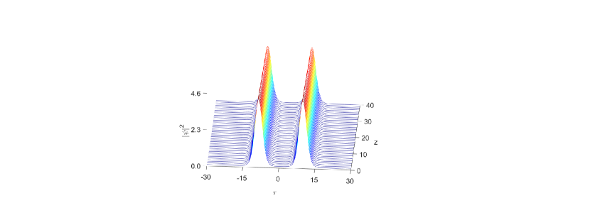
Figure 1: Propagation of the double-hump quartic soliton solution of Eq. (1) with parameters $\alpha=-2.0375,$ $\gamma=2.6,$ $\sigma=0.1,$ and $\epsilon=-0.1$.

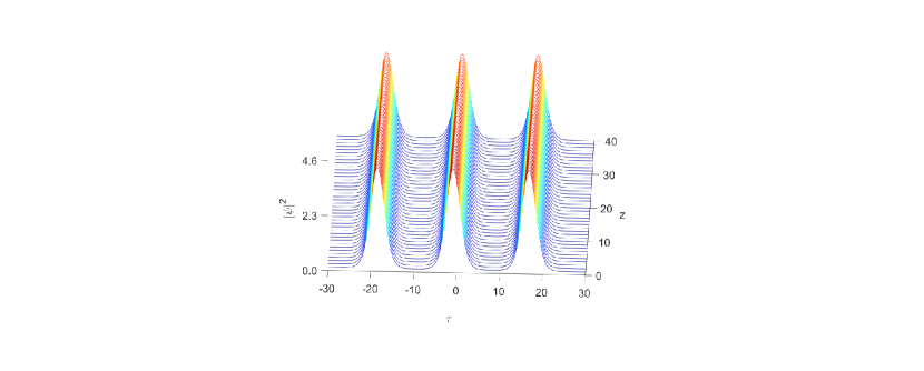
Figure 2: Propagation of the triple-hump quartic soliton solution of Eq. (1). The parameters are the same as in Fig. 1.

First, we analyze the existence of multiple-hump quartic soliton solutions of Eq. (1) and demonstrate that waveforms of double-, triple-, and quadruple-hump form can readily be generated in the fiber system. To perform a numerical study of multi-hump quartic solitons, we numerically integrated the full underlying equation (1) using the analytic soliton solution (8) with $N=2$ as an initial condition. The propagation of the double-hump quartic solitons calculated within the framework of Eq. (1) is shown in Fig. 1 for the parameter values: $\alpha=-2.0375,$ $\gamma=2.6,$ $\sigma=0.1,$ $\epsilon=-0.1,$ and $\xi_{0}=0.$ It should be noted that here, we have evaluated the dimensionless constant $a_{0}$ numerically as $a_{0}=3.$ From this figure, we see that the two humps are well separated and both of them have the same shape (width and maximum intensity). We also see that the wave profile remains unchanged after propagating a distance of forty normalized lengths. Assuming initial conditions in the form of the analytic soliton solution (8) containing three ($N=3$) or four ($N=4$) superimposed single-hump sech² solitons, we observe that both tripole and quadrupole quartic solitons are obtained, as shown in Figs. 2 and 3 respectively.

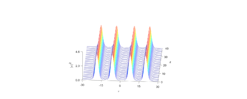
Figure 3: Propagation of the quadruple-hump quartic soliton solution of Eq. (1). The parameters are the same as in Fig. 1.

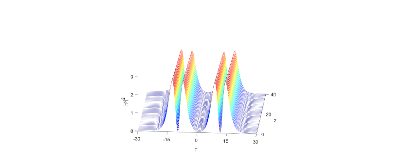
Figure 4: Propagation of the double-hump dipole soliton solution of Eq. (1) with parameters $\alpha=-1,$ $\gamma=-2.6,$ $\sigma=1.53,$ and $\epsilon=-0.25$.

This also indicates that these numerical findings agree excellently with our analytic solution (8). This physically important result implies that such multi-quartic solitons can be observed experimentally as long as the model (1) applies, thus implying that the solutions obtained here can be utilized for transmission.

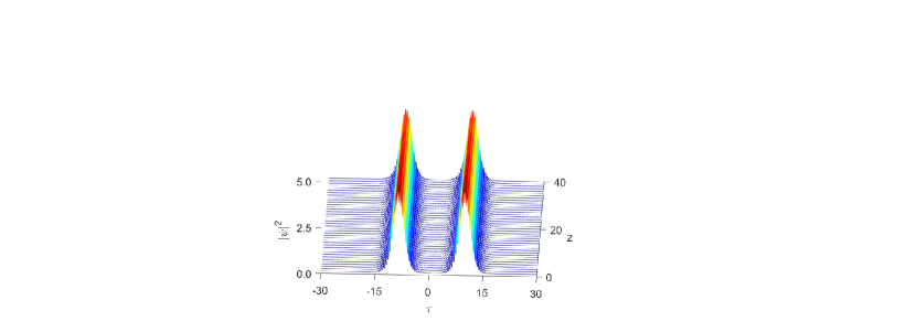
Figure 5: The numerical evolution of double-hump quartic solitons under the perturbation of white noise whose maximal value is $0.1$. The parameters are the same as those used in Fig. 1.

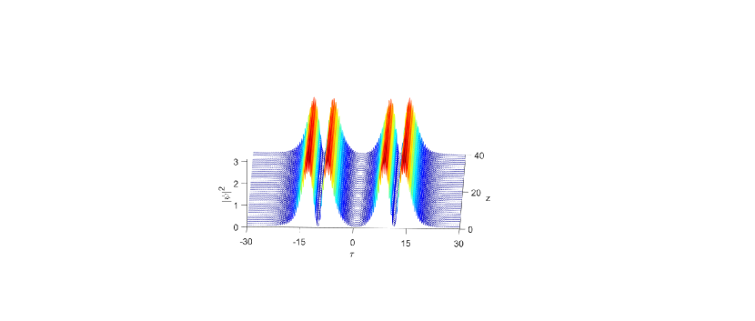
Figure 6: The numerical evolution of double dipole solitons under the perturbation of white noise whose maximal value is $0.1$. The parameters are the same as those used in Fig. 4.

Now we focus on the formation of the multiple-dipole soliton families in the fiber medium given analytically by Eq. (14). To obtain the numerical multi-hump solutions, we solved Eq. (1) by means of the split-step Fourier method for an input condition taking the form of the analytic soliton solution (14) with $N=2$. Here we have taken the following parameter values: $\alpha=-1,$ $\gamma=-2.6,$ $\sigma=1.53,$ $\epsilon=-0.25,$ and $\xi_{0}=0.$ We have also calculated the dimensionless constant $a_{0}$ numerically as $a_{0}=3.5.$ Figure 4 demonstrates that two dipole-type solitons may exist in the fiber medium. As seen, this double dipole-type soliton keeps its profile over a distance of forty normalized lengths. In addition to double dipole-type soliton modes, we have found that families of multiple-hump solutions can also be generated in the system, including coupled three, four, and N dipole-type soliton pulses.

V Numerical stability analysis

A distinguishing property of localized pulses is their stability to perturbations, as only stable solitons can be observed experimentally and utilized in physical applications. It is therefore important to analyze the stability of the obtained multiple-hump solutions with respect to small perturbations. Here, we take the numerically found double-hump quartic and dipole soliton solutions as examples to perform numerical experiments of the model (1). The numerical evolution of double-hump quartic and dipole soliton solutions under the perturbation of 10% white noise are depicted in Figs. 5 and 6, respectively. These results show that the multiple-hump soliton modes can propagate stably in the fiber system under the initial perturbation of the additive white noise. Hence we can conclude that the novel multi-soliton modes we obtained are stable.

VI Conclusions

We have presented the first analytical and numerical demonstration of the existence of multi-humped soliton pulses in a highly dispersive optical fiber exhibiting a Kerr nonlinearity. We revealed that in such nonlinear medium, the presence of cubic and quartic dispersions may lead to the coupling of quartic or dipole solitons into localized multi-hump pulses. The dynamics of the newly found solutions in the fiber material have been found to be very well modeled by the extended nonlinear Schrödinger equation incorporating the contributions of second-, third-, and fourth-order dispersions and self-phase modulation. The results demonstrate surprisingly that both quartic and dipole types of double-, triple-, and multi-humped soliton solutions can be formed in the fiber system. We have also demonstrated numerically that such soliton modes are stable with respect to small perturbations, thus implying that they can be utilized for transmission. To our knowledge, the multi-hump optical solitons obtained here for the extended NLSE are firstly reported in this work.

The discovery of such coupled multi-quartic and multi-dipole solitons represent an important advance in nonlinear optics. It should be mentioned that the newly found localized multi-solutions could find important application not only in optical fibers but also in other physical systems for which the underlying equation is applied for describing the wave dynamics. In future research problems, we shall take into consideration the absorption or amplification effects to expand the applicability of obtained multi-soliton solutions.

References

- (1) K. Porsezian and K. Nakkeeran, Phys. Rev. Lett. 76, 3955 (1996).
- (2) L. F. Mollenauer, R. H. Stolen, and J. P. Gordon, Phys. Rev. Lett. 45, 1095 (1980).
- (3) J. S. Aitchison, A. M. Weiner, Y. Silberberg, M. K. Oliver, J. L. Jackel, D. E. Leaird, E. M. Vogel, and P. W. E. Smith, Opt. Lett. 15, 471 (1990).
- (4) F. Salin, P. Grangier, G. Roger, and A. Brun, Phys. Rev. Lett. 56, 1132 (1986).
- (5) N.N. Akhmediev and S. Wabnitz, J. Opt. Soc. Am. B 9 (1992) 236-242.
- (6) G.I. Stegeman and M. Segev, Science 286, 1518 (1999).
- (7) S. L. Palacios, J. Opt. A: Pure Appl. Opt. 5, 180 (2003).
- (8) S. L. Palacios, J. M. Fernández-Díaz, Opt. Commun. 178, 457 (2000).
- (9) S. L. Palacios, J. M. Fernández-Díaz, J. Mod. Opt. 48, 1691 (2001).
- (10) A. Höök and M. Karlsson, Opt. Lett. 18, 1388 (1993).
- (11) M. Karlsson and A. Höök, Opt. Commun. 104, 303 (1994).
- (12) N. N. Akhmediev, A. V. Buryak, and M. Karlsson, Opt. Commun. 110, 540 (1994).
- (13) N. N. Akhmediev and A. V. Buryak, Opt. Commun. 121, 109 (1995).
- (14) A. V. Buryak and N. N. Akhmediev, Phys. Rev. E 51, 3572 (1995).
- (15) V. E. Zakharov and E. A. Kuznetsov, J. Exp. Theor. Phys. 86, 1035 (1998).
- (16) M. Piché, J.-F. Cormier, and X. Zhu, Opt. Lett. 21, 845 (1996).
- (17) Silicon Photonics, edited by L. Pavesi and D. J. Lockwood (Springer, New York, 2004).
- (18) B. Jalali, J. Lightwave Technol. 24, 4600 (2006).
- (19) Q. Lin, O. J. Painter, and G. P. Agrawal, Opt. Express 15, 16604 (2007).
- (20) A. D. Bristow, N. Rotenberg, and H. M. van Driel, Appl. Phys. Lett. 90, 191104 (2007).
- (21) J. Leuthold, C. Koos, and W. Freude, Nat. Photonics 4(8), 535 (2010).
- (22) S. Roy and F. Biancalana, Phys.Rev.A 87, 025801 (2013).
- (23) V. I. Kruglov and J. D. Harvey, Phys. Rev. A 98, 063811 (2018).
- (24) V. I. Kruglov, Opt. Commun. 472, 125866 (2020).
- (25) V. I. Kruglov and H. Triki, Phys. Rev. A 102, 043509 (2020).
- (26) H. Triki and V. I. Kruglov, Phys. Rev. E 101, 042220 (2020).
- (27) A. Choudhuri and K. Porsezian, Opt. Commun. 285, 364 (2012).
- (28) Y. Zhang, Z. Wang, Z. Nie, C. Li, H. Chen, K. Lu, and M. Xiao, Phys. Rev. Lett. 106, 093904 (2011).
- (29) M. Mitchell, M. Segev, and D. N. Christodoulides, Phys. Rev. Lett. 80, 4657 (1998).
- (30) A. Hasegawa and Y. Kodama, Solitons in Optical Communications (Oxford University Press, New York, 1995).
- (31) A. Blanco-Redondo, C. M. de Sterke, J. E. Sipe, T. F. Krauss, B. J. Eggleton, and C. Husko, Nat. Commun. 7, 10427 (2016).
- (32) G. P. Agrawal, Nonlinear Fiber Optics, 4th ed. (Academic, Boston, 2006).