MHVG2MTS: Multilayer Horizontal Visibility Graphs for Multivariate Time Series Analysis

?abstractname?

Understanding the properties of time-indexed multivariate data has been a predominant topic mainly to address open issues in multivariate time series analysis, such as finding appropriate measures to analyze temporal dependence and cross-dimension dependencies, as well as visualizing multidimensional data. Usually, the methodologies used to analyze multivariate time series are based on adapting approaches for univariate settings or on assumptions and parameters for specific problems. A different strategy uses complex network to obtain an additional and reduced representation of temporal and causal properties of the time series data. Recent strategies involve mapping multivariate time series into high-level network structures, specifically into multiplex networks representing interconnections between contemporary timestamps of different time series components.

In this work, we propose a new mapping method that takes advantage of the entire structure of multilayer networks. We introduce the multilayer horizontal visibility graph that is based on the new concept of cross-horizontal visibility between lagged timestamps of different components, which allows describing the cross-dimension dependencies via inter-layer edges. We use a set of existing topological measures of multilayer networks as well as a novel measure to evaluate and validate our approach, which is parameter-free, does not require data pre-processing and is applicable to any kind of multivariate time series data.

We provide an extensive experimental evaluation, where we explore the proposed topological measures, showing that the inter-layer edges based on cross-horizontal visibility preserve more information about the time series data after the mappings, information that would inevitably be lost using mapping methods that result in single-layer and multiplex structures. We also verify that the information mapped by the inter-layer edges is not enough on its own, but that it complements the data information captured by the commonly used intra-layer edges. Furthermore, we complement our analysis by performing a multivariate time series clustering task based on the proposed measure set of the proposed mapping method, demonstrating its validity.

Keywords: multivariate time series mappings, multilayer horizontal visibility graphs, multivariate time series features

1 Introduction

Recent technological developments led to the wide availability of large amounts of high dimensional time-indexed data for which appropriate methodological and computational tools are required. These multidimensional time-indexed data, usually designated as multivariate time series, have become ubiquitous in all domains from climate studies or health monitoring to financial data analysis, and are characterized by serial correlation as well as cross-sectional dependencies, in what is often designated as the curse of dimensionality.

To overcome the lack of appropriate methodological and computational tools to characterize high-dimensional time-indexed data, feature-based approaches for time series analysis have been proposed in the literature. Time series features are traditionally based on statistics and models for time series analysis and often rely on pre-processing and/or assumptions that are not usually satisfied. A particular methodology that is free of such requirements consists in mapping the time series into a complex network and then extracting topological features of the network for time series mining tasks and forecasting. In fact, network science, the research area that studies how to extract information from complex networks (Albert and Barabási,, 2002; Barabási,, 2016), provides a vast set of topological graph measurements (Costa et al.,, 2007), a well-defined set of problems such as community detection (Fortunato,, 2010) or link prediction (Lü and Zhou,, 2011), and a large track record of successful application of complex network methodologies to different fields (Vespignani,, 2018), including graph classification (Peach et al.,, 2021).

Univariate time series are mapped into single-layer networks based on the concepts of visibility, transition probability, and proximity (Zou et al.,, 2019; Silva et al.,, 2021). Multivariate time series may be mapped into single or multiple-layer networks. In the former, the nodes represent the component time series and the edges represent the relationships between the nodes (component time series) computed using statistical methods or models. These methods imply that all important information on the dynamics of each time series component, such as serial correlation, is lost in the mapping. Mapping methods that represent multivariate time series as multiplex networks were proposed with the objective of preserving both the dynamical (over time) and the cross-sectional information contained in the multivariate data (Lacasa et al.,, 2015; Eroglu et al.,, 2018; Silva et al.,, 2021). In these multiplex networks, each component univariate time series is mapped into a layer (using a univariate time series mapping in which each timestamp is represented by a node) and different layers are connected via the common nodes (time stamps). Inevitably, lagged cross-correlations, which sometimes are the most important information, are lost in the mapping process.

To overcome this limitation, we propose a new mapping to represent a multivariate time series as a multiple-layer complex network in this work. Multiple-layer networks, or multilayer networks, are complex structures capable of establishing internal connections (within the same layer) and external connections (between different layers) which allow the creation of very complete and flexible data structures (Kivelä et al.,, 2014). From a high-level view, multilayer networks have a structure compatible with that of multivariate time series. The proposed mapping is based on a new horizontal visibility concept, the cross-horizontal visibility, developed to capture the cross-dependencies between pairs of component time series. Thus, the multiplex visibility graphs (Lacasa et al.,, 2015) are extended with the incorporation of inter-layer edges established according to the cross-horizontal visibility between different nodes (time stamps). These new edges/connections can capture dependencies between different timestamps of different variables. The resulting networks are denoted as multilayer horizontal visibility graphs. Furthermore, we propose a set of global topological multilayer network features as a novel set of features for multivariate time series comprising: intra-layer topological features, inter-layer topological features, all-layer topological features, and relational features which are topological features that relate components of the network (such as layers or edges). Within relational features, we propose a new topological feature aimed at relating intra and inter-layer connections. These different subsets of topological features allow to analyze and compare the underlying properties of intra-layer and inter-layer edges, and to assess the contribution of the proposed mapping method in relation to the multiplex methods in the literature. This proposed methodology is represented in Figure 1.

?figurename? 1: Schematic diagram of the network-based features approach to time series mining tasks.

We use synthetic multivariate time series generated from a selected set of multivariate time series models to test and evaluate the framework proposed in this work.

1.1 Contributions

The main contributions of this work are as follows:

• We introduce a new method for mapping multivariate time series into a complete multilayer network structure. This mapping is based on the concept of horizontal visibility and on a multiplex visibility graph to take better advantage of the structural capacity of multilayer networks. As far as we know, the incorporation of inter-layer edges between different entities of multilayer networks has not been previously used in the literature to analyze multivariate time series data.

• We propose a new topological feature for multilayer networks and present a different set of multilayer network topological features selected for the analysis of the proposed mapping method and to reduce the dimensionality of the multivariate time series data. As far as we know, no other work presents different topological features of multilayer networks, based on their intra- and inter-layer edges, in the context of time series analysis.

• We also perform a detailed exploratory and empirical analysis of the different sets of features used in this work, showcasing its validity and usefulness.

1.2 Organization

We have organized this document as follows. Section 2 introduces the basic concepts of multivariate time series and multilayer networks, setting the notation for the remainder of the paper, and also presents the background on mapping methods useful for understanding the proposed method. Next, Section 3 presents the new concept of visibility between time series components and the new mapping multivariate time series proposed. In Section 4 we present the set of topological features that we extend to multilayer networks as well as the new proposed topological feature to multilayer networks. Section 5 presents a study of this mapping method via analysis of the corresponding feature set, in order to characterize the properties of the multivariate time series, also presents a multivariate time series clustering task as a validation of the proposed method. Finally, Section 6 presents the conclusions, some comments, and possible future work.

2 Background

This Section introduces the main concepts and notation necessary for the remainder of the paper.

2.1 Multivariate Time Series

An Univariate Time Series (UTS) is a sequence of (scalar) observations indexed by time $t,$ usually denoted by $\{{Y}_{t}\}_{t=1}^{T}.$ Unlike a random sample, such observations are ordered in time and usually present serial correlation that must be accounted for in the analysis. If at each time $t$ we obtain a vector of $m$ observations, $\boldsymbol{Y}_{t}=[Y_{1,t},Y_{2,t},\ldots,Y_{m,t}]^{\prime},$ where $\prime$ represents the transpose, then the data set $\boldsymbol{Y}=\{\boldsymbol{Y}_{t}\}_{t=1}^{T}$ is called a Multivariate Time Series (MTS). Henceforward, the UTS components of the MTS $\boldsymbol{Y}$ are denoted by $\boldsymbol{Y}^{\alpha}=[Y_{\alpha,1},Y_{\alpha,2},\ldots,Y_{\alpha,T}],$ $\alpha=1,\ldots,m$ and thus we can denote the MTS by its components, $\boldsymbol{Y}=\{Y^{\alpha}\}_{\alpha=1}^{m}.$ MTS data present not only serial correlation within each component, $\boldsymbol{Y}^{\alpha},$ but also a correlation between the different UTS’s, $\boldsymbol{Y}^{\alpha}$ and $\boldsymbol{Y}^{\beta}$ with $\alpha\neq\beta,$ both contemporaneous and lagged correlation. Thus, analyzing MTS depends on key dependence measures such as the autocorrelation function (ACF), which measures the linear predictability of a UTS,

$$\rho(s,t)=\mbox{\rm corr}(Y_{t},Y_{s})=\frac{\mbox{\rm cov}(Y_{s},Y_{t})}{\sqrt{\mbox{\rm var}(Y_{s})\mbox{\rm var}(Y_{t})}},$$ (1)

and the cross-correlation function (CCF), which measures the correlation between any two components of the MTS, $\alpha$ and $\beta,$ say, at times $s$ and $t,$

$$\rho_{\alpha,\beta}(s,t)=\mbox{\rm corr}(Y_{\alpha,s},Y_{\beta,t}).$$ (2)

Time series analysis refers to the collection of procedures developed to systematically solve the statistical problems posed by the serial correlation. There is a plethora of (linear and non-linear) statistical models in the literature adequate to describe the behavior of UTS (Shumway and Stoffer,, 2017). And although the theory of UTS extends naturally to the multivariate case, such as the mean, covariance, ACF, and CCF functions, new concepts arise. MTS analysis requires tools, methods, and models for mining information from multiple measurements which present both temporal and cross-sectional correlations.

2.2 Multilayer Networks

A graph (or network), $G$, is a mathematical structure defined by a pair $(V,E)$, where $V$ represents the set of nodes and $E$ the set of edges (connections) between pairs of nodes. Two nodes $v_{i}$ and $v_{j}$ are called neighbors if they are connected, $(v_{i},v_{j})\in E.$ If there is no direction from a source node to a target node the edges are undirected: $(v_{i},v_{j})\in E$ implies that $(v_{j},v_{i})\in E.$ A graph can be represented by an adjacency matrix, $\boldsymbol{A}$, and $A_{i,j}$ is $1$ when $(v_{i},v_{j})\in E$ and is $0$ otherwise.

A Multilayer Network (MNet) is a complete and general structure suitable for modeling multiple complex systems through their interactions, intra- and inter-systems. A MNet is generally defined as a quadruplet $M=(V_{M},E_{M},V,\boldsymbol{L})$ where $V$ and $\boldsymbol{L}$ represent the set of entities and the set of layers of $M$, respectively, and $V_{M}$ and $E_{M}$ represent the global sets of nodes and edges, respectively. The $V_{M}\subseteq V\times L_{1}\times\ldots\times L_{m}$, where $L_{\alpha}\in\boldsymbol{L}$ is an elementary layer, is a set of node-layer combinations in which a node is present in the corresponding layer $L_{\alpha}$. The $E_{M}\subseteq V_{M}\times V_{M}$ is the set of edges that contain the pairs of possible combinations of nodes and elementary layers (Kivelä et al.,, 2014). We denominate as intra-layer edges, the connections between nodes of the same layer, $(v_{i}^{\alpha},v_{j}^{\alpha}),$ and inter-layer edges the connections between nodes of different layers, $(v_{i}^{\alpha},v_{j}^{\beta})$ with $\alpha\neq\beta.$ Two particular cases of multilayer networks are the monoplex network when $m=1$ and $M$ reduces to a (single-layer) network, $G,$ and the multiplex network, when $M$ is a sequence of $m$ graphs, $\{G^{\alpha}\}_{\alpha=1}^{m}=\{(V^{\alpha},E^{\alpha})\}_{\alpha=1}^{m}$, usually with a node set common to all elementary layers, and inter-layer edges connecting only the counterpart nodes across the layers, that is connecting $(v_{i}^{\alpha},v_{i}^{\beta}),$ $\alpha\neq\beta$ (Boccaletti et al.,, 2014). Figure 2 exemplifies the representation of simple multilayer and multiplex networks.

(a) Multilayer Network

(b) Multiplex Network

?figurename? 2: An illustrative example of two toy multilayer networks with five entities, $V=\{1,2,3,4,5\},$ and two layers $\boldsymbol{L}=\{L_{1},L_{2}\}.$ (a) represents a toy multilayer network and (b) a toy multiplex network. Solid lines represent the intra-layer edges and dashed lines represent the inter-layer edges.
Source: Modified from Silva et al., (2021).

A node-aligned MNet has an associated adjacency tensor of order $4$, $\boldsymbol{\mathcal{A}},$ where the tensor element $\mathcal{A}_{i,j,\alpha,\beta}$ is 1 when $(v_{i}^{\alpha},v_{j}^{\beta})\in E_{M}$ and is $0$ otherwise (Kivelä et al.,, 2014). If the MNet is not node-aligned, we can consider empty nodes to complete the tensor structure. Another representation is obtained by flattening $\boldsymbol{\mathcal{A}}$ into a supra-adjacency matrix, $\boldsymbol{A}$, where intra-layer edges are associated with diagonal element blocks and inter-layer edges with off-diagonal element blocks. Figure 3 represents the supra-adjacency matrices of the networks illustrated in Figure 2. From these element blocks we can infer three types of subgraphs:

• intra-layer graphs, $G^{\alpha}$, represented by the square matrices of order $|V^{\alpha}|$ formed by the diagonal element blocks (intra-layer edges, $A_{i,j}^{\alpha}$), ie., $\left[\begin{smallmatrix}\boldsymbol{A}^{\alpha}&\boldsymbol{0}\\ \boldsymbol{0}&\boldsymbol{0}&\end{smallmatrix}\right]$,

• inter-layer graphs, $G^{\alpha,\beta}$, represented by the square matrices of order $|V^{\alpha}|+|V^{\beta}|$ constructed from off-diagonal element blocks (inter-layer edges, $A_{i,j}^{\alpha,\beta}$ and $A_{j,i}^{\beta,\alpha}$, and no intra-layer edges, $A_{i,j}^{\alpha}=0$ and $A_{i,j}^{\beta}=0$) , ie., $\left[\begin{smallmatrix}\boldsymbol{0}&\boldsymbol{A}^{\alpha,\beta}\\ \boldsymbol{A}^{\beta,\alpha}&\boldsymbol{0}\end{smallmatrix}\right]$, and

• all-layer graphs, $G^{\alpha,\beta}_{all}$, represented by the square matrices of size $|V^{\alpha}|+|V^{\beta}|$ constructed by both on and off-diagonal element blocks (intra-layer edges, $A_{i,j}^{\alpha}$ and $A_{i,j}^{\beta}$, and inter-layer edges, $A_{i,j}^{\alpha,\beta}$ and $A_{j,i}^{\beta,\alpha}$), ie., $\left[\begin{smallmatrix}\boldsymbol{A}^{\alpha}&\boldsymbol{A}^{\alpha,\beta}\\ \boldsymbol{A}^{\beta,\alpha}&\boldsymbol{A}^{\beta}\end{smallmatrix}\right]$.

(a) Multilayer Network

(b) Multiplex Network

?figurename? 3: An illustrative example of two supra-adjacency matrices. (a) a supra-adjacency matrix of a toy multilayer network and (b) a supra-adjacency matrix of a toy multiplex network. Colored blocks represent the intra-layer graphs and gray blocks represent the inter-layer graphs.

Network science has been a very useful tool to answer the most diverse problems in several scientific fields (Vespignani,, 2018). A large number of topological, statistical, spectral, and combinatorial properties metrics that extract information from networks are available in the literature (Albert and Barabási,, 2002; Barabási,, 2016; Costa et al.,, 2007; Peach et al.,, 2021; Silva et al.,, 2022). We can group these metrics into global, local, and ”intermediate” features. The first group quantifies properties involving all network elements, the second properties over a given node or edge, and the last properties that involve subsets of the network, such as subgraphs. These metrics used in monoplex contexts can be extended to MNets. Most of the common topological metrics can be extended straightforwardly to intra-layer metrics by just computing them over the intra-layer edges. These metrics can also be extended to the whole MNet, computing them over both intra-layer and inter-layer edges (Kivelä et al.,, 2014; Huang et al.,, 2021). Other approaches rely on measurements and properties in the tensor analysis literature (Kivelä et al.,, 2014).

2.3 Mapping Time Series into Complex Networks

In the last decade, several network-based time series analysis approaches have been proposed. These approaches are based on the mappings of univariate and multivariate time series into the network domain, either into single-layer or multiple-layer networks (Silva et al.,, 2021). The mappings proposed in the literature are essentially based on concepts of visibility, transition probability, proximity, time series models, and statistics (Silva et al.,, 2021; Zou et al.,, 2019). In this section, we review the concepts of visibility graphs that are required for the next section.

Visibility Graphs (VG) establish connections (edges) between the timestamps (nodes) using visibility lines between the observations, where nodes are associated with the natural ordering of observations. There are two native variants of this method, the Natural Visibility Graph (NVG) (Lacasa et al.,, 2008) and the Horizontal Visibility Graph (HVG) (Luque et al.,, 2009). The idea of these methods is that each UTS observation, $Y_{t}$, is seen as a vertical bar with a height equal to its numerical value and that these bars are laid in a landscape where (the top of) a bar is visible from (the tops of) other bars. Each timestamp, $t$, is mapped into a node, $v_{t},$ and the corresponding edges $(v_{i},v_{j})$, for $i,j=1\ldots T$, $i\neq j$, are established if there is a visibility line between the corresponding data bars that is not intercepted. Formally, in the NVG and HVG, two nodes $v_{i}$ and $v_{j}$ are connected if for all $t_{k},$ $t_{i}<t_{k}<t_{j},$ $(t_{k},Y_{k})$ satisfies

$$Y_{k}<Y_{j}+(Y_{i}-Y_{j})\frac{(t_{j}-t_{k})}{(t_{j}-t_{i})}$$ NVG (3)

$$Y_{k}<Y_{i}\quad\wedge\quad Y_{k}<Y_{j}$$ HVG. (4)

We give a simple illustration of these methods in Figure 4.

?figurename? 4: An illustrative example of the two visibility graph algorithms. (a) toy time series and corresponding visibility lines between data bars (observations). Solid pink lines represent the natural visibility lines corresponding to the NVG method, and dotted blue lines represent the horizontal visibility lines corresponding to the HVG method. (b) network generated by the corresponding mappings. The NVG is the graph with all edges, including the dashed pink edges, and the HVG is the subgraph that does not include these edges.
Source: Adapted from Silva et al., (2022).

VGs are always connected, each node $v_{i}$ sees at least its nearest neighbors, $v_{i-1}$ and $v_{i+1},$ are always undirected unless we consider the direction of the time axis, and are invariant under affine transformations of the data (Lacasa et al.,, 2008), each transformation $X_{t}=aY_{t}+b,$ for $a\in\mathbb{R},b\in\mathbb{R},$ and $t=1,\ldots,T,$ leads to the same VG (Silva et al.,, 2021).

Based on the definition of MNet, Lacasa and co-authors (Lacasa et al.,, 2015) proposed an extension of the visibility mapping for MTS analysis, the Multiplex Visibility Graphs (MVG). Formally, a MVG of $m$ layers, $M,$ is constructed so that layer set, $\{L_{\alpha}\}_{\alpha=1}^{m},$ corresponds to the NVGs (or HVGs), $\{G^{\alpha}\}_{\alpha=1}^{m},$ associated with the time series components, $\{Y^{\alpha}\}_{\alpha=1}^{m}.$ $M$ is represented by the adjacency matrix vector, $\boldsymbol{A}_{M},$ whose elements are the adjacency matrices of each layer, $\boldsymbol{A}_{M}=\{\boldsymbol{A}^{1},\boldsymbol{A}^{2},\ldots,\boldsymbol{A}^{m}\}$ with $A^{\alpha}_{i,j}=1$ if the nodes $v_{i}^{\alpha}$ and $v_{j}^{\alpha}$ are connected in layer $L_{\alpha}$ and is 0 otherwise. Figure 5 illustrates the method.

?figurename? 5: An illustrative example of the multiplex natural visibility graph algorithm. (a) displays a toy multivariate time series, $\boldsymbol{Y}=\{\boldsymbol{Y}^{1},\boldsymbol{Y}^{2},\boldsymbol{Y}^{3}\},$ (b) the corresponding multiplex network, with three layers generated by the multiplex natural visibility graph algorithm.

3 MHVG: a New Multivariate Time Series Mapping

Visibility methods have shown to be very promising in capturing time series characteristics reflecting local and global properties of the data, and not requiring pre-processing.

This section presents a new visibility algorithm to map an MTS into a multilayer horizontal visibility graph. This algorithm is based on a new visibility concept, cross-horizontal visibility which is an extension of the traditional horizontal visibility.

3.1 Cross-Horizontal Visibility

Consider two time series $\boldsymbol{Z}^{\alpha}=(Z_{\alpha,1},\ldots,Z_{\alpha,T})$ and $\boldsymbol{Z}^{\beta}=(Z_{\beta,1},\ldots,Z_{\beta,T})$ on the same scale. Two arbitrary data values $(t_{i},Z_{\alpha,t_{i}})$ and $(t_{j},Z_{\beta,t_{j}})$ are said to have cross-horizontal visibility, Cross-HV if

$$Z_{\alpha,t_{i}}\wedge Z_{\beta,t_{j}}>\max{\left(Z_{\alpha,t},Z_{\beta,t}\right)},\ \ \textrm{ for all }t,\ \ t_{i}<t<t_{j},\ \ i,j=1,\ldots,T,i\neq j.$$ (5)

This definition implies that all data values have Cross-HV to its neighbours and that the visibility is reciprocal, meaning that if $(t,Z_{\alpha,t})$ has Cross-HV to $(s,Z_{\beta,s}),$ then $(s,Z_{\beta,s}),$ has Cross-HV to $(t,Z_{\alpha,t}).$ The concept of cross-horizontal visibility, Cross-HV, is illustrated in Figure 6 with two toy time series and for the first four data points, with the bi-coloured lines indicating (the reciprocal) visibility between the corresponding time series.

?figurename? 6: Schematic diagram of the cross horizontal visibility concept. (a) Illustrates a toy bivariate time series $\boldsymbol{Z}^{yellow},\boldsymbol{Z}^{blue},$ (same scale) and the corresponding maximum time series; (b) represents the cross-horizontal visibility, Cross-HVG, by solid bi-color lines (yellow and blue) connecting the data bars of the time series components $\boldsymbol{Z}^{yellow}$ and $\boldsymbol{Z}^{blue},$ for the first four timestamps.

3.2 Multilayer Horizontal Visibility Graph

A Multilayer Horizontal Visibility Graph (MHVG) is obtained by mapping a MTS, $\boldsymbol{Y}=\{Y^{\alpha}\}_{\alpha=1}^{m}$, into a MNet structure, $M=(V_{M},E_{M},V,\boldsymbol{L})$, using the concepts of HV and Cross-HV, as follows. Each unique timestamp, $t$, is mapped into an unique entity in $V_{M}$ and each component time series, $\boldsymbol{Y}^{\alpha}$ is mapped into a layer, $L_{\alpha}\in\boldsymbol{L},$ $\alpha=1,\ldots,m,$ using the HVG method described in Section 2.3, thus establishing the intra-layer edges, $(v_{i}^{\alpha},v_{j}^{\alpha})\in E_{M},$ $i,j=1,\ldots,T,$ $i\neq j.$ Then inter-layer edges $(v_{i}^{\alpha},v_{j}^{\beta})\in E_{M},$ between any two layers $L_{\alpha}$ and $L_{\beta},$ $\alpha,\beta=1,\ldots,m,$ $\alpha\neq\beta$ and $i,j=1,\dots,T,$ $i\neq j$ are established using the Cross-HV described above in Section 3.1. Note that to establish Cross-HV all the time series $\boldsymbol{Y}^{\alpha},$ $\alpha=1,\ldots,m$ must be in the same scale which may require a pre-processing step of the data set $\boldsymbol{Y},$ comprising the Min-Max scaling of each time series. The mapping is illustrated in Figure 7, with toy bivariate time series, for the sake of simplicity.

?figurename? 7: Schematic diagram of the multilayer horizontal visibility graph algorithm: (a) original time series, (b) Min-Max re-scaled time series and maximum time series, (c) illustration of cross-HV with the edges between adjacent timestamps omitted for simplicity (detail for the first four timestamps), (d) cross-horizontal visibility graph: solid black lines represent the intra-layer edges (the HVGs), dashed lines the inter-layer edges (the Cross-HVGs) and the red lines highlight inter-layer edges between nodes corresponding to non-adjacent timestamps.

From the generated MHVG, we can identify the intra-layer graphs, $\{G^{\alpha}\}_{\alpha=1}^{m}$ and the inter-layer graphs, $G^{\alpha,\beta},$ for $\alpha,\beta=1,\ldots,m$ and $\alpha\neq\beta$. $\{G^{\alpha}\}_{\alpha=1}^{m}$ correspond to the HVG of each individual time series component and it is represented by the adjacency matrix $\boldsymbol{A}^{\alpha}$ with $A_{i,j}^{\alpha}=1$ if $(v_{i}^{\alpha},v_{j}^{\alpha})\in E_{M}$ and 0 otherwise. $G^{\alpha,\beta}$ corresponds to the cross-horizontal visibility graph (Cross-HVG) of each pair of different time series components and it is represented by the adjacency matrix $\boldsymbol{B}^{\alpha,\beta}=\left[\begin{smallmatrix}\boldsymbol{0}&\boldsymbol{A}^{\alpha,\beta}\\ \boldsymbol{A}^{\beta,\alpha}&\boldsymbol{0}\end{smallmatrix}\right]$ with $A_{i,j}^{\alpha,\beta}=1$ and $A_{j,i}^{\beta,\alpha}=1$ if $(v_{i}^{\alpha},v_{j}^{\beta})\in E_{M}$, and 0 otherwise.

Algorithm 1 describes the concept of Cross-HV and Algorithm 2 describes mapping a multivariate time series into a Multilayer Horizontal Visibility Graph. In the Appendix, we describe the auxiliary functions to support the implementation of the method, Algorithm 3 describes the function that creates an HVG, and Algorithm 4 describes the function that creates the inter-layer edges.

Input: Two rescaled time series, $\boldsymbol{Z}^{a}$ and $\boldsymbol{Z}^{b}$, ($\boldsymbol{tsA}$, $\boldsymbol{tsB}$), the corresponding layers, $L_{a}$ and $L_{b}$, ($\boldsymbol{layerA}$, $\boldsymbol{layerB}$), and the maximum time series, $\max{\left(\boldsymbol{Z}^{a},\boldsymbol{Z}^{b}\right)}$, ($\boldsymbol{tsMax}$)

Procedure  CHVG($tsA,tsB,tsMax,layerA,layerB$)

      

      1$T\leftarrow tsMax.size()$

        $\triangleright$ The time series lengths         

      

      for node $i$ in $layerA.\textnormal{{get\_Nodes(}}\textnormal{\emph{}}\textnormal{{)}}$ do

            

            for node $j$ from $i+1$ to $T$ in $layerB.\textnormal{{get\_Nodes(}}\textnormal{\emph{}}\textnormal{{)}}$ do

                   if node $i$ can ’see’ $j$ then

                        2 $mnet.\textnormal{{add\_Edge(}}\textnormal{\emph{i, j, layerA, layerB}}\textnormal{{)}}$

                          $\triangleright$ Add inter-layer edge $(v_{i}^{a},v_{j}^{b})$  

                        

                   end if

                  

             end for

            

            for node $j$ from $i-1$ to $0$ in $layerB.\textnormal{{get\_Nodes(}}\textnormal{\emph{}}\textnormal{{)}}$ do

                   if node $i$ can ’see’ $j$ then

                        3 $mnet.\textnormal{{add\_Edge(}}\textnormal{\emph{i, j, layerA, layerB}}\textnormal{{)}}$

                          $\triangleright$ Add inter-layer edge $(v_{i}^{a},v_{j}^{b})$  

                        

                   end if

                  

             end for

            

       end for

      

      4return

Algorithm 1 Cross-Horizontal Visibility Graph

Input: A set of time series components, $\{\boldsymbol{Y}^{a}\}_{a=1}^{m}$, ($\boldsymbol{mts}$)

Output: A multilayer network, $M$, ($\boldsymbol{mnet}$)

Procedure  MHVG($mts$)

      

      1$m\leftarrow mts.size()$

        $\triangleright$ The number of time series components

      2 $mnet\leftarrow\{\}$

        $\triangleright$ The empty MNet $M$                             

      3 $n\_mts\leftarrow\{\}$

        $\triangleright$ List to store the rescaled time        

      

        series components                             

      

      for $a\leftarrow 1$ to $m$ do

            4 $mnet.layers[a]\leftarrow\{\}$

              $\triangleright$ The empty layer $L_{a}$                           

            5 HVG(mts[a], mnet.layers[a])

              $\triangleright$ Map the time series $\boldsymbol{Y}^{a}$ on the HVG    

            

              $L_{a}$ (Eq. 4)                                       

            6 $n\_mts[a]\leftarrow\textnormal{{MinMax(}}\textnormal{\emph{mts[a]}}\textnormal{{)}}$

              $\triangleright$ Rescale time series $\boldsymbol{Z}^{a}$                    

            

       end for

      

      for $a\leftarrow 1$ to $m-1$ do

             for $b\leftarrow a+1$ to $m$ do

                  7 $tsMax\leftarrow\textnormal{{MaxTS(}}\textnormal{\emph{n\_mts[a], n\_mts[b]}}\textnormal{{)}}$

                    $\triangleright$ Get the maximum rescaled time series

                  8 CrossHVG(n_mts[a], n_mts[b], tsMax, mnet.layers[a], mnet.layers[b])

                    $\triangleright$ Map the pairwise time

                  

                    series $\boldsymbol{Z}^{a}$ and $\boldsymbol{Z}^{b}$      

                  

                    on Cross-HVG (Eq. 5)  

                  

             end for

            

       end for

      

      9return $mnet$

Algorithm 2 Multilayer Horizontal Visibility Graph

4 A Novel Set of Multivariate Time Series Features

Mapping time series into complex networks and then using network topological features as features in univariate time series mining tasks has become a popular approach due to its dimensionality reduction capabilities (Silva et al.,, 2022; Fulcher,, 2018; Wang et al.,, 2006).

In this work, we propose a set of MHVG topological features to analyze MTS data which includes: i) common topological features extended to MNets and ii) a new feature constructed for MNets.

4.1 Topological features extended to MNets

Common network topological features such as node centrality, graph distances, clustering, and community can be naturally extended to a MNet structure and all the subgraphs mentioned in Section 2.2. To illustrate, consider a local centrality measure such as the degree $k_{i}$ of a node $v_{i}$, which represents the number of its adjacent edges. In a MNet, we can compute three variants of $k_{i},$ for each layer $\alpha=1,\ldots,m$ where we use the symbol $\prec$ (and $\preceq$) to express the inter-layer edges from a ”source” layer, $\alpha$ (and including intra-layer edges of the ”source” layer) to a ”destination” layer, $\beta,$

• intra-layer degree: $k_{i}^{\alpha}=\sum_{j}{A_{ij}^{\alpha}}$

• inter-layer degree: $k_{i}^{\alpha\prec\beta}=\sum_{j}{A_{ij}^{\alpha,\beta}}$

• all-layer degree: $k_{i}^{\alpha\preceq\beta}=k_{i}^{\alpha}+k_{i}^{\alpha\prec\beta}$

with $\beta\neq\alpha.$ Note that local inter and all-layer topological measurements are asymmetric measures, that is, $k_{i}^{\alpha\prec\beta}\neq k_{i}^{\beta\prec\alpha}$ and $k_{i}^{\alpha\preceq\beta}\neq k_{i}^{\beta\preceq\alpha}$, since the measure is relative to node-layer $v_{i}^{\alpha}$ or node-layer $v_{i}^{\beta}$.

In general, any common (local) topological feature $F_{i}$ can be easily extended to intra-layer features, $F_{i}^{\alpha}$, just computing them over individual layers, to inter-layer features, $F_{i}^{\alpha\prec\beta}$, computing over inter-layer edges, and to all-layer features, $F_{i}^{\alpha\preceq\beta}$, which compute over both intra-layer and inter-layer edges.

An important feature associated with the degree is the degree distribution $P(k)$ that measures the fraction of nodes in a graph with degree $k$. In this work, we analyze the three variants of degree distributions, $P(k^{\alpha}),P(k^{\alpha\prec\beta})$ and $P(k^{\alpha\preceq\beta})$, in layer $L_{\alpha},\alpha=1,\ldots,m$, associated with its intra-layer degree, inter-layer degree and all-layer degree, respectively.

To measure the similarity between pairs of layers in an MNet, we also use the Jensen–Shannon divergence ($JSD$) which measures the distance between two distributions. As an example, the $JSD$ between intra-layer degree distributions $P(k^{\alpha})$ and $P(k^{\beta})$, ($JSD^{\alpha,\beta}_{intra}$) is defined as follows:

$$JSD(P(k^{\alpha})||P(k^{\beta}))=\frac{1}{2}KLD(P(k^{\alpha})||Q(k))+\frac{1}{2}KLD(P(k^{\beta})||Q(k))$$

where $Q(k)=\frac{1}{2}(P(k^{\alpha})+P(k^{\beta}))$ and $KLD$ is the Kullback–Leibler divergence:

$$KLD(P(k^{\alpha})||Q(k))=\sum_{k}{P(k^{\alpha})\log_{2}\left(\frac{P(k^{\alpha})}{Q(k)}\right)}.$$

Similarly, we define $JSD$ for the inter-layer degree distributions ($JSD_{inter}^{\alpha,\beta}$) and the all-layer degree distributions ($JSD_{all}^{\alpha,\beta}$). Note that $JSD$ is a symmetrical version of the asymmetrical measure $KLD$. In the remainder of this work, we will refer to similarity measures, such as $JSD$, as relational features.

In addition, we also extend global topological features to MNets. These features involve all (sub)graph elements and therefore are symmetric. As an example, consider the average degree $\bar{k}$ which calculates the arithmetic mean of the degree $k_{i}$ of all nodes in the graph. As before, we can compute three variants of $\bar{k}$ in a MHVG,

• average intra-degree: $\bar{k}^{\alpha}=\frac{1}{|V_{\alpha}|}\sum_{i}{k_{i}^{\alpha}}$

• average inter-degree: $\bar{k}^{\alpha,\beta}=\frac{1}{|V_{\alpha}|+|V_{\beta}|}\left(\sum_{i}{k_{i}^{\alpha\prec\beta}}+\sum_{j}{k_{j}^{\beta\prec\alpha}}\right)$

• average all-degree: $\bar{k}^{\alpha,\beta}_{all}=\frac{1}{|V_{\alpha}|+|V_{\beta}|}\left(\sum_{i}{k_{i}^{\alpha\preceq\beta}}+\sum_{j}{k_{j}^{\beta\preceq\alpha}}\right)$

In short, we can compute a (global) topological feature $\boldsymbol{F}$ in the subgraphs of the MNet: intra ($\boldsymbol{F}^{\alpha}$), inter ($\boldsymbol{F}^{\alpha,\beta}$), and all-layer graphs ($\boldsymbol{F}^{\alpha,\beta}_{all}$).

Motivated by the set of features proposed in Silva et al., (2022), namely based on the concepts of node centrality, graph distances, clustering, and community and the three types of MNet measurements defined above, we propose intra-layer, inter-layer, and all-layer, for each pair of layers, features as follows:

• Average Degree: the average intra-degree $\bar{k}^{\alpha}$, average inter-degree $\bar{k}^{\alpha,\beta}$ and average all-degree $\bar{k}^{\alpha,\beta}_{all}$, as formulated above.

• Average path length: geodesic distances $d_{i,j},i\neq j$ between node $v_{i}$ and $v_{j}$ corresponding to the length of the shortest paths between them, where the path length is the number of edges in the path. The average (intra-/inter-/all-)path length ($\bar{d}^{\alpha},\bar{d}^{\alpha,\beta}$ and $\bar{d}^{\alpha,\beta}_{all}$) is the arithmetic mean of the shortest paths among all pairs of nodes in (intra, inter, and all-layer) graph.

• Number of communities: The number of (intra-/inter-/all-)communities, ($S^{\alpha},S^{\alpha,\beta}$ and $S^{\alpha,\beta}_{all}$), is the amount of groups/communities of nodes that are densely connected on the subgraph. These communities are found by performing random walks on the subgraph (intra, inter, and all-layer graph), so that short random walks tend to stay in the same community until the modularity value (defined below) cannot be increased anymore.

• Modularity: (Intra-/Inter-/All-)modularity, ($Q^{\alpha},Q^{\alpha,\beta}$ and $Q^{\alpha,\beta}_{all}$), measures how good a specific division of the corresponding subgraph $G$ is into (intra-/inter-/all-)communities.

Table 1 provides the formulation details.

4.2 Ratio Degree: a new MNet topological feature

The ratio degree is a new topological feature for multilayer graphs, introduced here to relate intra-layer and inter-layer visibility.

The ratio degree of node $v_{i}^{\alpha}$ of layer $L^{\alpha}$ is defined as

$$r_{i}^{\alpha\preceq\beta}=\frac{k_{i}^{\alpha\prec\beta}}{k_{i}^{\alpha}}$$ (6)

for any layer $L^{\beta}.$ The average ratio degree, $\bar{r}^{\alpha\preceq\beta}$, is the arithmetic mean of the ratio degree of the nodes of layer $L^{\alpha}.$ Note that the ratio degree is asymmetric, and thus it is not necessarily true that $\bar{r}^{\alpha\preceq\beta}=\bar{r}^{\beta\preceq\alpha}$.

4.3 The MHVG Features Set

The set of features defined above and summarized in Table 1 forms a set of features extracted from MHVG, as depicted in Figure 8, that we propose to characterize a MTS.

?tablename? 1: Topological multilayer network features .

Feature	Formulation	Note
Average Degree	$\displaystyle\bar{k}^{\alpha}=\frac{1}{N_{\alpha}}\sum_{i}{k_{i}^{\alpha}}$
	$\displaystyle\bar{k}^{\alpha,\beta}=\frac{1}{N_{\alpha,\beta}}\left(\sum_{i}{k_{i}^{\alpha\prec\beta}}+\sum_{j}{k_{j}^{\beta\prec\alpha}}\right)$
	$\displaystyle\bar{k}^{\alpha,\beta}_{all}=\frac{1}{N_{\alpha,\beta}}\left(\sum_{i}{k_{i}^{\alpha\preceq\beta}}+\sum_{j}{k_{j}^{\beta\preceq\alpha}}\right)$
Degree Distribution	$\displaystyle P(k^{\alpha})=\frac{n_{k^{\alpha}}}{N_{\alpha}}$	$n$: number of nodes $v_{i}^{\alpha}$ with the corresponding degree $k$
	$\displaystyle P(k^{\alpha\prec\beta})=\frac{n_{k^{\alpha\prec\beta}}}{N_{\alpha}}$
	$\displaystyle P(k^{\alpha\preceq\beta})=\frac{n_{k^{\alpha\preceq\beta}}}{N_{\alpha}}$
Average Path Length	$\displaystyle\bar{d}^{\alpha}=\frac{1}{N_{\alpha}(N_{\alpha}-1)}\sum_{i\neq j}{d_{i,j}^{\alpha}}$	$d_{i,j}$: length of the shortest paths between $v_{i}$ and $v_{j}$ in the corresponding subgraph
	$\displaystyle\bar{d}^{\alpha,\beta}=\frac{1}{N_{\alpha,\beta}(N_{\alpha,\beta}-1)}\sum_{i\neq j}{d_{i,j}^{\alpha,\beta}}$
	$\displaystyle\bar{d}^{\alpha,\beta}_{all}=\frac{1}{N_{\alpha,\beta}(N_{\alpha,\beta}-1)}\sum_{i\neq j}{d_{i,j,all}^{\alpha,\beta}}$
Number of Communities	$\displaystyle S^{\alpha}=|\mathcal{C}^{\alpha}|$	$\mathcal{C}$: set of communities in corresponding subgraph
	$\displaystyle S^{\alpha,\beta}=|\mathcal{C}^{\alpha,\beta}|$
	$\displaystyle S^{\alpha,\beta}_{all}=|\mathcal{C}^{\alpha,\beta}_{all}|$
Modularity	$\displaystyle Q^{\alpha}=\frac{1}{2|E^{\alpha}|}\sum_{i,j}{\left[B_{i,j}-\frac{k_{i}k_{j}}{2|E^{\alpha}|}\right]}\delta\left(c_{i},c_{j}\right)$	$\displaystyle\boldsymbol{B}=\boldsymbol{A}^{\alpha}$
	$\displaystyle Q^{\alpha,\beta}=\frac{1}{2|E^{\alpha,\beta}|}\sum_{i,j}{\left[B_{i,j}-\frac{k_{i}k_{j}}{2|E^{\alpha,\beta}|}\right]}\delta\left(c_{i},c_{j}\right)$	$\boldsymbol{B}=\left[\begin{smallmatrix}\boldsymbol{0}&\boldsymbol{A}^{\alpha,\beta}\\ \boldsymbol{A}^{\beta,\alpha}&\boldsymbol{0}\end{smallmatrix}\right]$
	$\displaystyle Q^{\alpha,\beta}_{all}=\frac{1}{2|E^{\alpha,\beta}_{all}|}\sum_{i,j}{\left[B_{i,j}-\frac{k_{i}k_{j}}{2|E^{\alpha,\beta}_{all}|}\right]}\delta\left(c_{i},c_{j}\right)$	$\boldsymbol{B}=\left[\begin{smallmatrix}\boldsymbol{A}^{\alpha}&\boldsymbol{A}^{\alpha\beta}\\ \boldsymbol{A}^{\beta\alpha}&\boldsymbol{A}^{\beta}\end{smallmatrix}\right]$
Jensen–Shannon Divergence	$\displaystyle JSD_{intra}^{\alpha,\beta}=JSD(P(k^{\alpha})||P(k^{\beta}))$
	$\displaystyle JSD_{inter}^{\alpha,\beta}=JSD(P(k^{\alpha\prec\beta})||P(k^{\beta\prec\alpha}))$
	$\displaystyle JSD_{all}^{\alpha,\beta}=JSD(P(k^{\alpha\preceq\beta})||P(k^{\beta\preceq\alpha}))$
Average Ratio Degree	$\displaystyle\bar{r}^{\alpha\preceq\beta}=\frac{1}{|N_{\alpha}|}\sum_{i}{r_{i}^{\alpha\preceq\beta}}$

?figurename? 8: Schematic diagram of the multilayer network features set extraction process. A multivariate time series $\boldsymbol{Y}$ is mapped into a multilayer horizontal visibility graph. And for each of its subgraphs (intra-layer, inter-layer, and all-layer graphs) are computer the global topological features ($\bar{k},\bar{d},S,Q$ and $P(k)$) and relational features ($\bar{r}$ and $JSD$).

5 Empirical evaluation of MHVG

In this section, we investigate whether the mapping method and the features set introduced above are useful for characterizing MTS data and evaluate the performance of the methodology for MTS mining tasks. We use synthetic bivariate time series, generated from bivariate time series models to control for MTS correlation (serial and cross) properties. First, we make some considerations about the implementation of the methodology.

5.1 Implementation Details

The mapping and topological features proposed in this work do not, conceptually, depend on the implementation details. However, to show the practicality of the proposed method and to provide the reader with the ability to reproduce it, we describe in more detail how we computed our methodology, illustrated in Figure 8. Note that for illustrative purposes, we used $m=2$, but the method is extensible to any value of $m$.

To map a multivariate time series $\boldsymbol{Y}$ into an MHVG, we follow Algorithm 2. The intra-layer HVG’s, $\{G^{\alpha}\}_{\alpha=1}^{m}$, for each time series component, $\{Y_{\alpha,t}\},\alpha=1,\ldots,m,t=1,\ldots,T$, are created using the implemented Algorithm 3 proposed in (Luque et al.,, 2009). And the inter-layer edges are added following the mapping method based on cross-horizontal visibility criteria proposed in Section 3.1, and using the implemented Algorithm 4. Subgraphs corresponding to intra-, inter-, and all-layers, are fixed via corresponding adjacency submatrices of the MHVG (see Sections 2.2). And the corresponding topological features described above are computed using the methodologies and algorithms described below.

The average degree ($\bar{k}$) and average ratio degree ($\bar{r}$) are calculated by the arithmetic mean of the degrees $k_{i}$ and ratio degrees $r_{i}$, respectively, of all node $v_{i}$ in the respective subgraph. In this work, the average path length ($\bar{d}$) follows an algorithm that computes the average shortest path length between all pairs of nodes (of respective subgraphs) using a breadth-first search algorithm. To calculate the number of communities ($S$), the function used makes use of the known ”Louvain” algorithm that finds community structures by multi-level optimization of modularity ($Q$) feature (see Blondel et al., (2008) for more details). And the degree distributions ($P(k)$) and Jensen–Shannon divergence ($JSD$) are implemented as described above section.

We used C++ and its needed set of libraries (such as igraph and standard libraries) to implement the data structure to store an MNet and compute the functions to extract the topological features. For reproducibility purposes, the datasets and results are made available in https://github.com/vanessa-silva/MHVG2MTS.

5.2 Synthetics Datasets

We consider a set of six bivariate time series models ($m=2$), denoted by Data Generating Processes (DGPs), summarized in Table 2. These MTS models present a set of particular characteristics in terms of serial and cross-correlation (see Section2.1), namely: white noise (WN) processes simulate noise effects , one process does not present any kind of correlation, and the other presents strong contemporaneous correlation; vector autoregression (VAR) processes simulate smooth linear data, presenting both serial and cross-correlation; vector generalized autoregressive conditional heteroskedasticity (VGARCH) processes simulate nonlinear data with persistent periods of high or low volatility. The parameters of each DGP are chosen so that the data exhibits a range of serial and cross-correlation properties as described in Table 2. A detailed description of the DGP and their properties as well as computational details are presented in Appendix B.

For each DGP in Table 2, we generated 100 instances of length $T=10000$. As illustrated in Figure 8, we map each bivariate time series into an MHVG, highlight the intra-, inter-, and all-layer graphs, and extract the corresponding topological features.

?tablename? 2: Synthetic data generating processes (bivariate time series models). Parameters, the main characteristic of the data sets, and notation are also included. See Appendix B for more details.

DGP	Parameters	Characteristics	Notation
Independent White Noise	$\displaystyle\boldsymbol{\epsilon}_{t}\sim N(0,1)$	Noise effect No correlation	iBWN
Correlated White Noise	$\displaystyle\bigl{[}\begin{smallmatrix}\epsilon_{1,t}\\ \epsilon_{2,t}\end{smallmatrix}\bigr{]}\sim N\left(0,\bigl{[}\begin{smallmatrix}1.00&0.86\\ 0.86&1.50\end{smallmatrix}\bigr{]}\right)$	Noise effect No serial correlation Cross-correlation	cBWN
Weak VAR$(1)$	$\displaystyle\boldsymbol{\varphi}=\bigl{[}\begin{smallmatrix}2.50\\ 0.50\end{smallmatrix}\bigr{]},\boldsymbol{\phi}=\bigl{[}\begin{smallmatrix}0.20&0.10\\ 0.02&0.10\end{smallmatrix}\bigr{]}$	Weak correlation (serial and cross)	wVAR
	$\displaystyle\boldsymbol{\epsilon}_{t}\sim\bigl{[}\begin{smallmatrix}1.00&0.10\\ 0.10&1.50\end{smallmatrix}\bigr{]}$
Strong VAR$(1)$	$\displaystyle\boldsymbol{\varphi}=\bigl{[}\begin{smallmatrix}0\\ 0\end{smallmatrix}\bigr{]},\boldsymbol{\phi}=\bigl{[}\begin{smallmatrix}0.70&0.02\\ 0.30&0.80\end{smallmatrix}\bigr{]}$	Strong correlation (serial and cross, lagged and contemporaneous)	sVAR
	$\displaystyle\boldsymbol{\epsilon}_{t}\sim\bigl{[}\begin{smallmatrix}1.00&0.86\\ 0.86&1.50\end{smallmatrix}\bigr{]}$
Weak VGARCH$(1,1)$	$\displaystyle\boldsymbol{\omega}=\bigl{[}\begin{smallmatrix}0.05\\ 0.02\end{smallmatrix}\bigr{]}$, $\boldsymbol{\alpha}=\bigl{[}\begin{smallmatrix}0.10&0.00\\ 0.00&0.05\end{smallmatrix}\bigr{]}$	No serial correlation Weak cross-correlation	wGARCH
	$\displaystyle\boldsymbol{\beta}=\bigl{[}\begin{smallmatrix}0.85&0.00\\ 0.00&0.88\end{smallmatrix}\bigr{]},\boldsymbol{\epsilon}_{t}\sim\bigl{[}\begin{smallmatrix}1.00&0.10\\ 0.10&1.50\end{smallmatrix}\bigr{]}$
Strong VGARCH$(1,1)$	$\displaystyle\boldsymbol{\omega}=\bigl{[}\begin{smallmatrix}0.05\\ 0.02\end{smallmatrix}\bigr{]}$, $\boldsymbol{\alpha}=\bigl{[}\begin{smallmatrix}0.10&0.00\\ 0.00&0.05\end{smallmatrix}\bigr{]}$	Strong contemporaneous cross-correlation	sGARCH
	$\displaystyle\boldsymbol{\beta}=\bigl{[}\begin{smallmatrix}0.85&0.00\\ 0.00&0.88\end{smallmatrix}\bigr{]},\boldsymbol{\epsilon}_{t}\sim\bigl{[}\begin{smallmatrix}1.00&0.86\\ 0.86&1.50\end{smallmatrix}\bigr{]}$

To illustrate the procedure, we represent in Figure 9 one instance with 300 observations of each DGP and the corresponding cross-correlation (CCF) plot (first two columns of the plot), the intra-, inter-, and all-layers degree distributions on a semi-logarithmic scale (last three columns of the plot). These degree distributions are computed as the arithmetic mean of the degree distributions of the 100 simulated instances. The plots clearly show that the degree distributions are different across the DGPs. In fact, Luque et al., (2009) has shown that the intra-layer degree distribution for white noise (uncorrelated data) follows a power law $\left(P(k)=\frac{1}{3}\left(\frac{2}{3}\right)^{k-2}\right)$ and our results indicate that strong serial correlation leads to intra-layer degree distributions that are positively skewed: as illustrated in Appendix B, the sVAR is the only DGP that produces data with strong serial correlation. The degree distribution for the inter-layer subgraphs does not have an algebraic close form even in the simplest case of two uncorrelated white noises. However, extensive simulations indicate that it does not follow the power law $P(k)=\frac{1}{3}\left(\frac{2}{3}\right)^{k-2}$, as illustrated in the first line, the third column of Figure 9. The plots also indicate that inter-layer degree distribution depends both on the correlation between the two time series (CCF represented in the second column of the plot in Figure 9) and the serial correlation within each time series. Moreover, we note that inter-layer degree distributions for sVAR are positively skewed, for GARCH models, wGARCH and sGARCH, are exponentially shaped while the remaining are approximately linear. Once again, a slower decay of the lagged correlation leads to a longer tail in the degree distribution. Also, the degree distribution curves corresponding to the GARCH models stand out from the others, especially the inter- and all-layer degree distributions. The exponential shape of the inter-layer degree distributions is induced by the heteroscedasticity and volatility clusters in the data which limit cross-horizontal visibility to the nearest neighbours.

?figurename? 9: Analysis plots of DGP. The first column shows a subset of timestamps of each DGP, the second plots the cross-correlation function between their corresponding time series components, and the last three show the degree distribution of the MHVGs. The plots corresponding to the degree distributions are on a semi-logarithmic scale. Lines of different colors refer to each DGP model ($\boldsymbol{Y}$), where the darkest colors refer to their first components ($\boldsymbol{Y}^{1}$) and the lighter ones to the second ($\boldsymbol{Y}^{2}$).

5.3 MTS features via MHVG

The results for all the 21 features introduced in Section 4 and all DGPs, organized by subgraph structure, are summarized, mean (standard deviation), in Tables 3 and 4. The values have been Min-Max normalized (across models) for comparison purposes since the range of the different features varies across the different DGPs. The cells in the tables are coloured with a gradient based on the mean values: cells with a maximum value of 1 are coloured red, cells with a minimum value of 0 are coloured white, and the remainder with a hue of red colour proportional to its value.

?tablename? 3: Mean values (standard deviation) of the $100$ instances of each DGP for each topological global feature from intra-layer graphs, $G^{1}$ and $G^{2}$, and inter-layer graph, $G^{1,2}$, resulting from the corresponding MHVGs.

DGP	Average			Average			Number of			Modularity
	Degree			Path Length			Communities
	$\bar{k}^{1}$	$\bar{k}^{2}$	$\bar{k}^{1,2}$	$\bar{d}^{1}$	$\bar{d}^{2}$	$\bar{d}^{1,2}$	$S^{1}$	$S^{2}$	$S^{1,2}$	$Q^{1}$	$Q^{2}$	$Q^{1,2}$
iBWN	0.805	0.756	0.615	0.044	0.049	0.012	0.265	0.312	0.206	0.150	0.207	0.319
	(0.081)	(0.077)	(0.033)	(0.019)	(0.023)	(0.024)	(0.083)	(0.083)	(0.064)	(0.055)	(0.056)	(0.093)
cBWN	0.802	0.752	0.940	0.045	0.050	0.007	0.260	0.310	0.126	0.150	0.196	0.181
	(0.083)	(0.080)	(0.078)	(0.022)	(0.022)	(0.015)	(0.084)	(0.090)	(0.080)	(0.051)	(0.062)	(0.141)
wVAR	0.790	0.759	0.615	0.058	0.056	0.009	0.342	0.338	0.211	0.287	0.277	0.308
	(0.079)	(0.090)	(0.033)	(0.022)	(0.025)	(0.016)	(0.093)	(0.100)	(0.062)	(0.058)	(0.062)	(0.099)
sVAR	0.561	0.601	0.683	0.449	0.328	0.011	0.791	0.700	0.195	0.893	0.857	0.263
	(0.121)	(0.108)	(0.092)	(0.050)	(0.039)	(0.025)	(0.104)	(0.121)	(0.069)	(0.046)	(0.064)	(0.103)
wVGARCH	0.540	0.554	0.102	0.380	0.325	0.252	0.239	0.282	0.696	0.185	0.207	0.669
	(0.159)	(0.140)	(0.135)	(0.136)	(0.097)	(0.188)	(0.104)	(0.083)	(0.212)	(0.057)	(0.081)	(0.210)
sVGARCH	0.542	0.505	0.146	0.390	0.385	0.232	0.234	0.300	0.670	0.179	0.212	0.626
	(0.184)	(0.186)	(0.174)	(0.138)	(0.149)	(0.217)	(0.103)	(0.105)	(0.220)	(0.065)	(0.065)	(0.240)

?tablename? 4: Mean values (standard deviation) for each topological global and relational features from all-layer graphs, $G^{1,2}_{all}$, resulting from MHVGs of DGP, computed over the $100$ instances of each DGP.

DGP	Average	Average	Num. of	Modular.	Average		Jensen–Shannon
	Degree	Path L.	Comm.		Ratio Deg.		Divergence
	$\bar{k}^{1,2}_{all}$	$\bar{d}^{1,2}_{all}$	$S^{1,2}_{all}$	$Q^{1,2}_{all}$	$\bar{r}^{1\preceq 2}$	$\bar{r}^{2\preceq 1}$	$JSD^{\alpha,\beta}_{intra}$	$JSD^{\alpha,\beta}_{inter}$	$JSD^{\alpha,\beta}_{all}$
iBWN	0.617	0.042	0.237	0.338	0.586	0.582	0.170	0.034	0.090
	(0.033)	(0.018)	(0.107)	(0.052)	(0.028)	(0.037)	(0.071)	(0.0355)	(0.047)
cBWN	0.940	0.051	0.382	0.507	0.942	0.931	0.166	0.061	0.244
	(0.078)	(0.018)	(0.087)	(0.064)	(0.071)	(0.084)	(0.079)	(0.076)	(0.236)
wVAR	0.616	0.054	0.305	0.413	0.565	0.571	0.207	0.034	0.096
	(0.033)	(0.022)	(0.107)	(0.049)	(0.032)	(0.034)	(0.074)	(0.041)	(0.051)
sVAR	0.682	0.457	0.457	0.842	0.574	0.579	0.682	0.120	0.314
	(0.092)	(0.04955)	(0.127)	(0.05673)	(0.106)	(0.091)	(0.128)	(0.148)	(0.225)
wVGARCH	0.104	0.297	0.310	0.206	0.103	0.097	0.154	0.085	0.075
	(0.134)	(0.065)	(0.108)	(0.076)	(0.136)	(0.127)	(0.065)	(0.110)	(0.065)
sVGARCH	0.147	0.388	0.431	0.3954	0.149	0.145	0.149	0.114	0.137
	(0.173)	(0.120)	(0.118)	(0.088)	(0.179)	(0.170)	(0.077)	(0.161)	(0.172)

The results indicate that each set of features - intra-layer (first two columns of each feature in Table 3), inter-layer (third column of each feature in Table 3), all-layer (first four columns of Table 4) and relational (last five columns of Table 4) - distinguishes two groups of MTS depending on properties pertaining to correlation (serial and cross) and volatility clustering.

To understand which MNet topological features capture the specific properties of the MTS models, we perform PCA on the feature space. Figure 10 represents a bi-plot obtained using the intra-, inter-, all-layer, and relational features, with the two principal components (PC) explaining $83.8\%$ of the variance. The bi-plots resulting from PCA in restricted feature sets are represented in Figure 14 (Appendix B). Overall, we can say that the average degree and average ratio degree, $\bar{k}$ and $\bar{r}$, are positively and negatively correlated, respectively, with the average path length, $\bar{d}$. The community-related features of the intra- and all-layer graphs are positively correlated but less correlated with the community-related features of the inter-layer graphs. The features that most contribute to the first two PCs are the $\bar{k}^{1,2},S^{1,2}$ and $Q^{1,2}$ of the inter-layer graphs, the $\bar{k}^{1,2}_{all}$ of the all-layer graphs, the $\bar{r}^{1\preceq 2}$ and $\bar{r}^{2\preceq 1}$ of the relational layers, and $Q^{1}$ and $Q^{2}$ of the intra-layer graphs (see Figure 15 of Appendix B).

?figurename? 10: Bi-plot of the first two principal components (PC) of principal component analysis for the Data Generating Process (DGP). Each DGP is represented by a different color and the arrows represent the contributions of the MNet features to the PCs, the larger the size, sharpness, and closer to the red the greater the contribution of the feature. Features set together are positively correlated and those placed on opposite quadrants are negatively correlated.

Figure 10 clearly shows four groups of models, GARCH, sVAR, cBWN and a group constituted by the wVAR and the iBWN and identifies the topological features that characterize them.

The strong ACF and CCF of the sVAR are represented by high values for the number of communities and modularity in its intra- and all-layer graphs. Inter-layer graphs present higher values of community-related features for GARCH models. The average path length represents the GARCH models, in particular, the average path length of the all-layer graphs tries to distinguish both wGARCH and sGARCH. The strong contemporaneous CCF of the cBWN is represented by high values of average ratio degree features, such as the average degree values of its inter and all-layer graphs. The iBWN and wVAR, are represented by high values of intra-layer average degree.

The above results indicate that the topological features extracted from MHVG are adequate as a set of MTS features. To further explore this idea, we proceed with clustering analysis of the DGPs via MNet topological features.

5.4 Mining Time Series with MNetF

In this section, we illustrate the usefulness of MNet features in MTS data mining tasks with a case study regarding DGP clustering via a feature-based approach (Maharaj et al.,, 2019). Given a set of MTS, we compute the MNet feature vectors, which are then Min-Max rescaled into the $[0,1]$ range and organized in a feature data matrix. The PCs are computed, with no need for z-score normalization in PCA computation, and finally, a clustering algorithm, the k-means, is applied to all PCs. We opt for k-means since it is fast and widely used in the literature, but it requires the pre-introduction of the number of clusters, which for the purpose of this work is not a problem. We use the appropriate evaluation metrics: Average Silhouette (AS), Adjusted Rand Index (ARI), and Normalized Mutual Information (NMI). The AS does not need the ground truth, while the ARI and NMI do. The range of values for NMI is $[0,1]$ and for ARI and AS is $[-1,1]$. The results are summarized in Figure 11.

(a) ARI

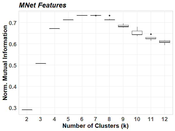
(b) NMI

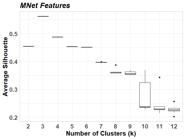
(c) AS

?figurename? 11: Results of DGP’s clustering evaluations using the three evaluation metrics, ARI, NMI, and AS, for the different number of clusters, $k$, given as input in the $k$-means algorithm. The results refer to 10 repetitions of the clustering analysis using the MNet features set.

As illustrated in Figure 11, the different metrics indicate different number of clusters for the data set: ARI indicates $k=5$ followed by $k=6$ which is the ground truth value, while the NMI indicates either $k=6$ or $k=7.$ Metric AS, using the silhouette method to assess the quality of the clusters indicates $k=3.$ It is interesting to note that the elements of the three clusters are: the sVAR models in one cluster, the GARCH models in another, and the WN and wVAR models in the third cluster, indicating that the DGPs were clustered according to correlation (serial and cross) and volatility properties.

Figure 12 represents the results from clustering the 100 instances of the 6 DGPs, using the 21 MNet features and the $k$-means algorithm with $k=6.$ It is noticeable the perfect attribution of cBWN and sVAR samples across two different clusters (clusters 1 and 3), the attribution of iBWN and wVAR samples across the same cluster (cluster 2), and a homogeneous attribution of GARCH samples (wGARCH and sGARCH) across two clusters (4 and 5), and some samples of cBWN and sGARCH across cluster 6 since $k=6$ and the GARCH samples are the most disparate in the feature space.

?figurename? 12: Attribution of the samples corresponding to instances of MTS models to the different clusters, according to intra, inter, all-layer, and relational feature set. The different models are represented on the horizontal axis and by a unique color. The bivariate time series samples are represented by the colored points according to its model process. The vertical axis represents the cluster number to which a bivariate time series is assigned.

The clustering exercise was performed considering subsets of the MNet feature set. The results summarized in Table 5 indicate that inter-layer edges contain, in fact, information about the MTS, leading to better clustering results.

Subgraphs with both intra-layer edges and inter-layer edges add information that leads to improvements in the clustering results (compare the last three rows of the Table with the first two). The results show that cross-HVG of inter-layer edges capture different properties from MTS data, that, as we expected, translate into better clustering results. Also note that the results of ARI and NMI from the set of intra-layer features are good results, because the DGP under analysis involves the same statistical process for the two time series components whose properties inherent to each process are also captured by the HVG mapping methods.

?tablename? 5: Clustering evaluation metrics for the different clustering analyses resulting from different MNet feature vectors. The values reflect the mean of 10 repetitions of the proposed method for different feature vectors and for the ground truth ($k=6$). The highest values are highlighted.

Feature Set	ARI	NMI	AS
	$[-1,1]$	$[0,1]$	$[-1,1]$
Intra-layer	0.522	0.614	0.289
Inter-layer	0.294	0.418	0.508
All-layer	0.667	0.725	0.505
Relational	0.575	0.646	0.622
MNet	0.629	0.713	0.452

6 Conclusions

In this paper, we propose a new mapping method to represent multivariate time series as multilayer networks. Our procedure relies on two main steps: first each time series component is mapped into a layer in a multilayer networks structure, following the horizontal visibility concept available in the literature, and for each pair of time series components in the multivariate time series, inter-layer edges are established based on a new concept of cross-horizontal visibility proposed in this work. We are interested in analyzing the concept of horizontal visibility as the base concept, given the promising results achieved in the previous works (Silva,, 2018; Silva et al.,, 2022), but the idea of the proposed mapping method, the Cross-(H)VG algorithm, naturally extends to the concept of natural visibility and other versions of VG’s.

To assess the proposed method, we analyzed a specific set of topological features of multilayer networks. These features are based on concepts of node centrality, graph distances, clustering, communities, and similarity measures. Each feature extracted from all the subgraphs of the resulting multilayer network structure: intra-layer graphs (only intra-layer edges), inter-layer graphs (only inter-layer edges) and all-graphs (with both intra and inter-layer edges).

We perform an empirical evaluation on a set of 600 synthetic bivariate time series, grouped in 6 different and specific statistical models, that result in a data set of 600 MHVGs. To understand the potential of our proposed mapping method, we first analyze the degree distributions of the intra, inter, and all-layer subgraphs of MHVGs. We were able to identify the specific properties of multivariate time series models, namely, we were able to relate weak and strong cross-correlation with shapes of the inter-layer degree distribution curves and weak and strong autocorrelation with shapes of the intra-layer degree distribution curves. In particular, we were also able to relate the persistence of strong correlations to distributions (that result in positively skewed shape) that have a longer right tail. Adding to the correlation properties (both auto and cross, contemporaneous and lagged), the properties of the statistical models, such as heteroscedasticity and smoothness, results in inter and all-layer degree distributions with different shape curves.

We also investigated the global features of the subgraphs (intra, inter, and all-layer). Community-related features from intra and all-layer graph highlight the strongly VAR models, with high and persistent autocorrelation and cross-correlation, as well as with smoothness, and from inter-layer graphs highlight the heteroscedasticity models, both weak and strong VGARCH models. However, the values of average path length from all-layer graphs seem to distinguish the properties of weakly and strongly correlated. The average intra-degree has higher values for independent white noise and weak VAR models, but not distinguishing them.

The new relational feature proposed in this work, average ratio degree, seems to differentiate well the highly correlated contemporary white noise models, which leads to a similarity in its inter-layer degree and intra-layer degree features. In the context of this work, based on the synthetic models chosen for analysis, the Jensen–Shannon divergence measure is only useful to characterize strong VAR models that present very strong and very persistent correlations, unlike the other models. However, this feature can be quite useful in real contexts, where the different variables of a multivariate time series can follow different dynamic models that will be captured by this feature. We intend to investigate this and other characteristics, as well as other topological features of multilayer networks in our future works.

To further showcase the validity of the proposed mapping method and feature set, we perform a clustering analysis of the synthetic bivariate time series. The results allow concluding that features that use the inter-layer edges of the MHVGs add valuable information to intra-layer features thus allowing to distinguish of the different statistical processes underlying the multivariate data models.

To conclude, this work proposes a procedure to map multivariate time series into multilayer networks as a mean to obtain a set of multivariate time series features that can be used for mining tasks. Open issues for future work are new topological features of multilayer networks and a more extensive empirical study with benchmark multivariate time series.

Availability of data and materials

The raw data are available at https://github.com/vanessa-silva/MHVG2MTS.

?appendixname? A MHVG: Algorithms

Input: A time series, $\boldsymbol{Y}^{a}$, ($\boldsymbol{ts}$), and a layer, $L_{a}$, ($\boldsymbol{layer}$)

Procedure  HVG($ts,layer$)

      

      1$T\leftarrow ts.size()$

        $\triangleright$ The time series length              

      

      for $i\leftarrow 1$ to $T$ do

            2 $mnet.\textnormal{{add\_Node(}}\textnormal{\emph{i, layer}}\textnormal{{)}}$

              $\triangleright$ Add node-layer $v_{i}^{a}$ corresponding

            

              to timestamp $t_{i}$                          

            

       end for

      

      for $i\leftarrow 1$ to $T-1$ do

            3 $mnet.\textnormal{{add\_Edge(}}\textnormal{\emph{i, i+1, layer}}\textnormal{{)}}$

              $\triangleright$ Add intra-layer edge $(v_{i}^{a},v_{i+1}^{a})$   

            4 $k\leftarrow 1$

            for $j\leftarrow 2$ to $T-i$ do

                  5 $condition\leftarrow ts[i+k]$

                  6 $p\leftarrow ts[i+j]$

                   /* Test HVG condition: Eq. 4 */

                   if $condition\geq ts[i]$ then

                        7 $break$

                        

                   else if $condition<p$ then

                        8 $mnet.\textnormal{{add\_Edge(}}\textnormal{\emph{i, i+j, layer}}\textnormal{{)}}$

                          $\triangleright$ Add intra-layer edge $(v_{i}^{a},v_{i+j}^{a})$   

                        9 $k\leftarrow j$

                        

                  

             end for

            

       end for

      

      10return

Algorithm 3 Horizontal Visibility Graph

Input: Two rescaled time series, $\boldsymbol{Z}^{a}$ and $\boldsymbol{Z}^{b}$, ($\boldsymbol{tsA}$, $\boldsymbol{tsB}$), the corresponding layers, $L_{a}$ and $L_{b}$, ($\boldsymbol{layerA}$, $\boldsymbol{layerB}$), and the maximun time series, $\texttt{max}\left(\boldsymbol{Z}^{a},\boldsymbol{Z}^{b}\right)$,($\boldsymbol{tsMax}$)

Procedure  CHVG($tsA,tsB,tsMax,layerA,layerB$)

      

      1$T\leftarrow tsMax.size()$

        $\triangleright$ The time series lengths         

      

      /* Test cross-horizontal visibility to the right of $Y_{a,i}$ */

       for $i\leftarrow 1$ to $T-1$ do

            2 $k\leftarrow i+1$

            for $j\leftarrow i+1$ to $T$ do

                   if $j=i+1$ then

                        3 $mnet.\textnormal{{add\_Edge(}}\textnormal{\emph{i, i+1, layerA, layerB}}\textnormal{{)}}$

                          $\triangleright$ Add inter-layer edge $(v_{i}^{a},v_{i+1}^{b})$

                        

                   else

                        4 $condition\leftarrow tsMax[k]$

                        5 $p\leftarrow tsB[j]$

                         /* Test Cross-HVG condition: Eq. 5 */

                         if $condition\geq tsA[i]$ then

                              6 $break$

                              

                         end if

                        if $condition<p$ then

                              7 $mnet.\textnormal{{add\_Edge(}}\textnormal{\emph{i, j, layerA, layerB}}\textnormal{{)}}$

                                $\triangleright$ Add inter-layer edge $(v_{i}^{a},v_{j}^{b})$  

                              8 $k\leftarrow j$

                              

                         else if $condition<tsMax[j]$ then

                              9 $k\leftarrow j$

                                $\triangleright$ Update index $k$ when $tsMax[j]>tsMax[k]$

                              

                         end if

                        

                   end if

                  

             end for

            

       end for

      

      /* Test cross-horizontal visibility to the left of $Y_{a,i}$ */

       for $i\leftarrow 2$ to $T$ do

            10 $k\leftarrow i-1$

            for $j\leftarrow i-1$ to $1$ do

                   if $j=i-1$ then

                        11 $mnet.\textnormal{{add\_Edge(}}\textnormal{\emph{i, i-1, layerA, layerB}}\textnormal{{)}}$

                          $\triangleright$ Add inter-layer edge $(v_{i}^{a},v_{i-1}^{b})$

                        

                   else

                        12 $condition\leftarrow tsMax[k]$

                        13 $p\leftarrow tsB[j]$

                         /* Test Cross-HVG condition: Eq. 5 */

                         if $condition\geq tsA[i]$ then

                              14 $break$

                              

                         end if

                        if $condition<p$ then

                              15 $mnet.\textnormal{{add\_Edge(}}\textnormal{\emph{i, j, layerA, layerB}}\textnormal{{)}}$

                                $\triangleright$ Add inter-layer edge $(v_{i}^{a},v_{j}^{b})$  

                              16 $k\leftarrow j$

                              

                         else if $condition<tsMax[j]$ then

                              17 $k\leftarrow j$

                                $\triangleright$ Update index $k$ when $tsMax[j]>tsMax[k]$

                              

                         end if

                        

                   end if

                  

             end for

            

       end for

      

Algorithm 4 Cross-Horizontal Visibility Graph

?appendixname? B Multivariate Time Series Models

Main references Cipra, (2020); Wei, (2019); Shumway and Stoffer, (2017); Tsay, (2013).

Linear Models

BWN

The vector white noise process, $\boldsymbol{\epsilon}_{t},$ is a vector of sequences of i.i.d. random variables with mean vector 0 and and covariance matrix function $\boldsymbol{\Sigma}$, where $\boldsymbol{\Sigma}$ is an $m\times m$ symmetric positive definite matrix. The components of the white noise process are serially uncorrelated $\mbox{\rm corr}(\epsilon_{i,t},\epsilon_{i,s})=0,$ for $t\neq s$, but may be contemporaneously correlated, $\mbox{\rm corr}(\epsilon_{i,t},\epsilon_{j,t})\neq 0$. It is the simplest multivariate time series process that reflects information that is neither directly observable nor predictable. We generate white noise processes, $\boldsymbol{\epsilon}_{t}\sim N(0,1)$, that are not correlated, that is, are independent, and we refer to theses processes as iBWN, and white noise processes contemporaneously correlated that we refer to them as cBWN, $\bigl{[}\begin{smallmatrix}\epsilon_{1,t}\\ \epsilon_{2,t}\end{smallmatrix}\bigr{]}\sim N\left(0,\bigl{[}\begin{smallmatrix}1.00&0.86\\ 0.86&1.50\end{smallmatrix}\bigr{]}\right)$.

VAR$(1)$

The vector autoregression process is a natural extension of the univariate autoregressive (AR) process that the variable values depends linearly on its own previous values and on a stochastic term. We defined a VAR$(1)$ process as a vector AR process of order 1 if it satisfies the following equation:

$$\boldsymbol{Y}_{t}=\boldsymbol{\varphi}+\boldsymbol{\phi}\boldsymbol{Y}_{t-1}+\boldsymbol{\epsilon}_{t},$$ (7)

where $\boldsymbol{\epsilon}_{t}$ is the vector white noise, $\boldsymbol{\phi}$ is the vector of autoregressive constants and $\boldsymbol{\varphi}$ is the vector of intercepts. We generate a VAR$(1)$ of 2 dimensions with the following vector of parameters:

$$\bigl{[}\begin{smallmatrix}Y_{1,t}\\ Y_{2,t}\end{smallmatrix}\bigr{]}=\bigl{[}\begin{smallmatrix}\varphi_{1,1}\\ \varphi_{2,1}\end{smallmatrix}\bigr{]}+\bigl{[}\begin{smallmatrix}\phi_{1,1}&\phi_{1,2}\\ \phi_{2,1}&\phi_{2,2}\end{smallmatrix}\bigr{]}\bigl{[}\begin{smallmatrix}Y_{1,t-1}\\ Y_{2,t-1}\end{smallmatrix}\bigr{]}+\bigl{[}\begin{smallmatrix}\epsilon_{1,t}\\ \epsilon_{2,t}\end{smallmatrix}\bigr{]},$$ (8)

where $\boldsymbol{\varphi}=\bigl{[}\begin{smallmatrix}2.50\\ 0.50\end{smallmatrix}\bigr{]}$, $\boldsymbol{\phi}=\bigl{[}\begin{smallmatrix}0.20&0.10\\ 0.02&0.10\end{smallmatrix}\bigr{]}$ and $\boldsymbol{\epsilon}_{t}\sim\bigl{[}\begin{smallmatrix}1.00&0.10\\ 0.10&1.50\end{smallmatrix}\bigr{]}$ to generate weakly correlated VAR$(1)$ processes, and $\boldsymbol{\varphi}=\bigl{[}\begin{smallmatrix}0\\ 0\end{smallmatrix}\bigr{]}$, $\boldsymbol{\phi}=\bigl{[}\begin{smallmatrix}0.70&0.02\\ 0.30&0.80\end{smallmatrix}\bigr{]}$ and $\boldsymbol{\epsilon}_{t}\sim\bigl{[}\begin{smallmatrix}1.00&0.86\\ 0.86&1.50\end{smallmatrix}\bigr{]}$ to generate strongly correlated VAR$(1)$ processes. We refer to the two models generated as wVAR and sVAR, respectively.

Non Linear Models

VGARCH$(1,1)$

Also generalized autoregressive conditional heteroskedasticity (GARCH) models can be generalized to multidimensional settings, extending the principle of univariate conditional heteroscedasticity to mutual volatility. We generate a bivariate GARCH$(1,1)$ model according to the following volatility equation:

$$\boldsymbol{\sigma}_{t}=\boldsymbol{\omega}+\boldsymbol{\alpha}\boldsymbol{\epsilon^{2}}_{t-1}+\boldsymbol{\beta}\boldsymbol{\sigma}_{t-1},$$ (9)

where $\boldsymbol{\sigma}_{t}$ denotes the volatility in the variables $\boldsymbol{Y}_{t}$. We generate a VGARCH$(1,1)$ of 2 dimensions with the following vector of parameters:

$$\bigl{[}\begin{smallmatrix}\sigma_{11,t}\\ \sigma_{22,t}\end{smallmatrix}\bigr{]}=\bigl{[}\begin{smallmatrix}\omega_{1,1}\\ \omega_{2,1}\end{smallmatrix}\bigr{]}+\bigl{[}\begin{smallmatrix}\alpha_{1,1}&\alpha_{1,2}\\ \alpha_{2,1}&\alpha_{2,2}\end{smallmatrix}\bigr{]}\bigl{[}\begin{smallmatrix}\epsilon^{2}_{1,t-1}\\ \epsilon^{2}_{2,t-1}\end{smallmatrix}\bigr{]}+\bigl{[}\begin{smallmatrix}\beta_{1,1}&\beta_{1,2}\\ \beta_{2,1}&\beta_{2,2}\end{smallmatrix}\bigr{]}\bigl{[}\begin{smallmatrix}\sigma_{11,t}\\ \sigma_{22,t}\end{smallmatrix}\bigr{]},$$ (10)

where $\boldsymbol{\epsilon}_{t}\sim\bigl{[}\begin{smallmatrix}1.00&0.10\\ 0.10&1.50\end{smallmatrix}\bigr{]}$ to generate weakly correlated VGARCH$(1,1)$ processes, and $\boldsymbol{\epsilon}_{t}\sim\bigl{[}\begin{smallmatrix}1.00&0.86\\ 0.86&1.50\end{smallmatrix}\bigr{]}$ to generate strongly correlated VGARCH$(1,1)$ processes. To both processes we use $\boldsymbol{\omega}=\bigl{[}\begin{smallmatrix}0.05\\ 0.02\end{smallmatrix}\bigr{]}$, $\boldsymbol{\alpha}=\bigl{[}\begin{smallmatrix}0.10&0.00\\ 0.00&0.05\end{smallmatrix}\bigr{]}$ and $\boldsymbol{\beta}=\bigl{[}\begin{smallmatrix}0.85&0.00\\ 0.00&0.88\end{smallmatrix}\bigr{]}$. We refer to the two models generated as wGARCH and sGARCH, respectively.

Bivariate time series are generated from the above DGP using the R packages: lgarch (Sucarrat,, 2015), mAr (Barbosa,, 2012) and ccgarch (Nakatani,, 2014).

B.1 Autocorrelation Function Plots

See Figure 13.

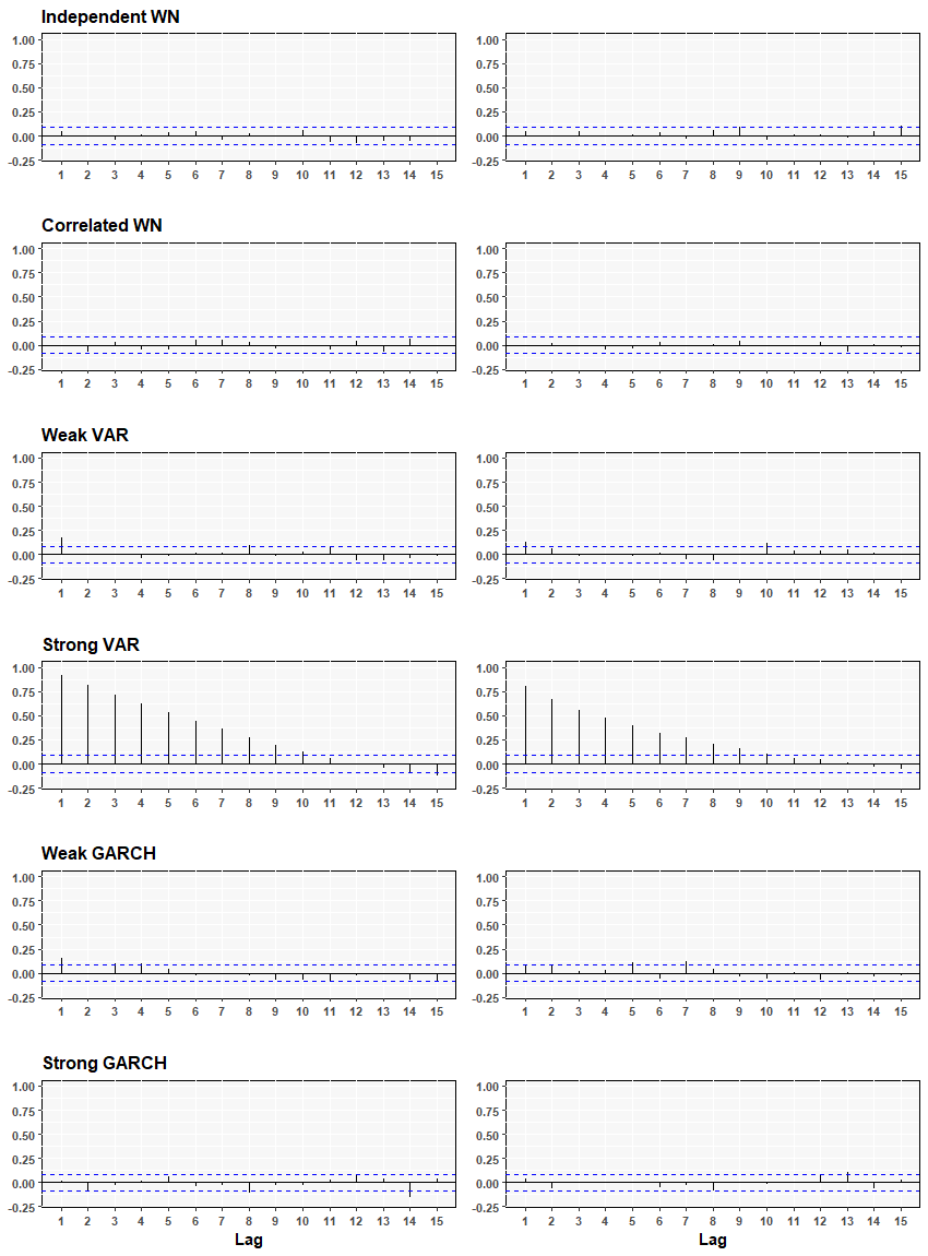
?figurename? 13: Plot of the autocorrelation function of an instance of each of the DGP models. The first column refers to the ACF’s of the first time series component ($\boldsymbol{Y}_{1}$) of each model, while the second column refers to the second component ($\boldsymbol{Y}_{2}$).

B.2 Principal Component Analysis Results

See Figure 14 and Figure 15.

(a) Intra-layer features

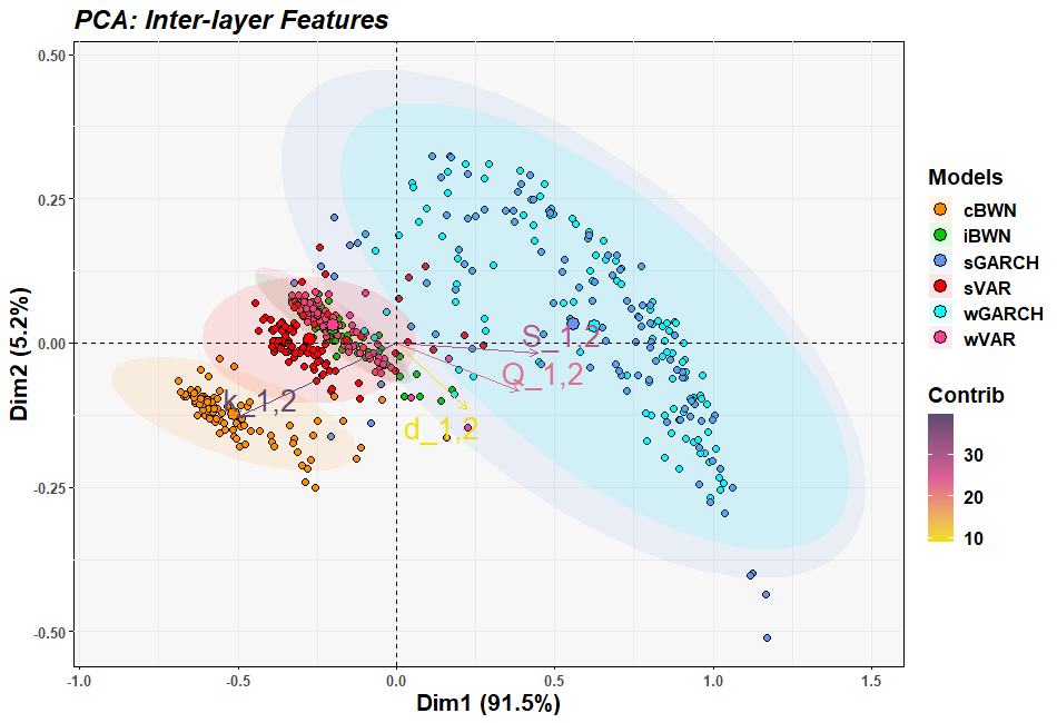
(b) Inter-layer features

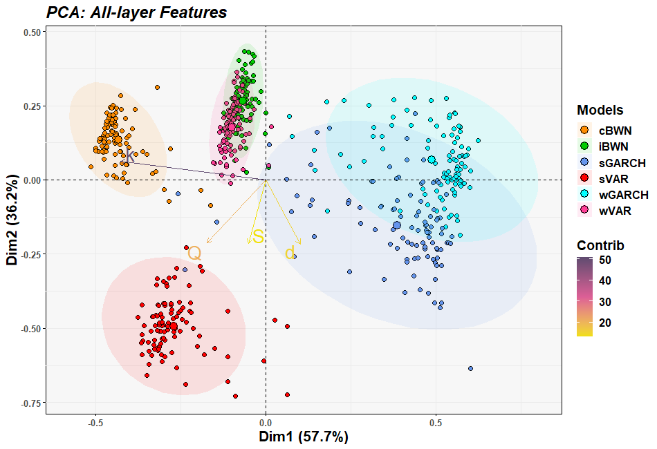
(c) All-layer features

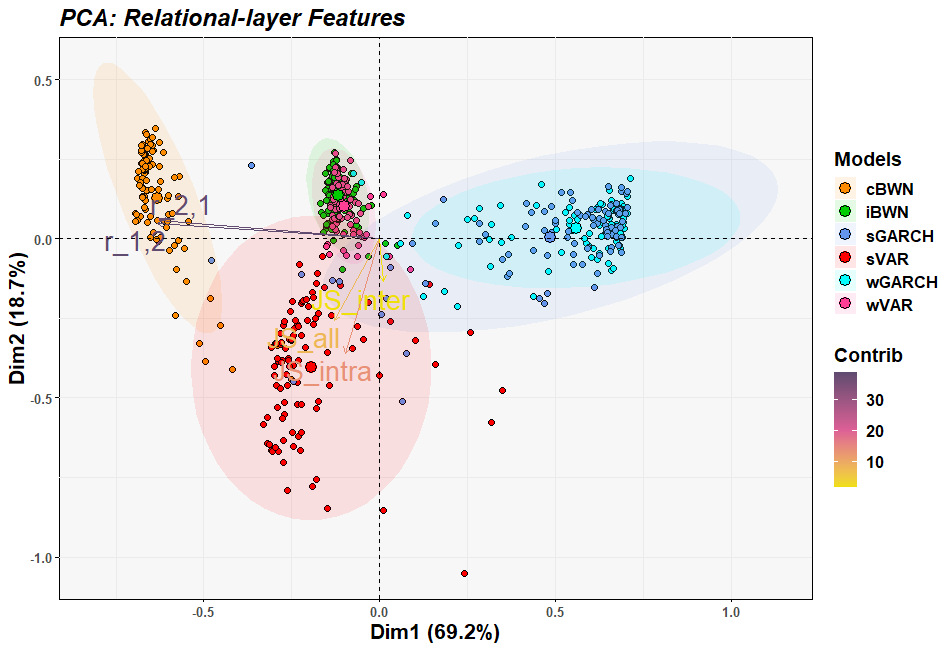
(d) Relational features

?figurename? 14: Bi-plot of the first two principal components (PC) of principal component analysis for the Data Generating Process (DGP) using the different feature vectors. Each DGP is represented by a different color and the arrows represent the contributions of the set of features to the PC’s, the larger the size, sharpness, and closer to the red the greater the contribution of the feature.

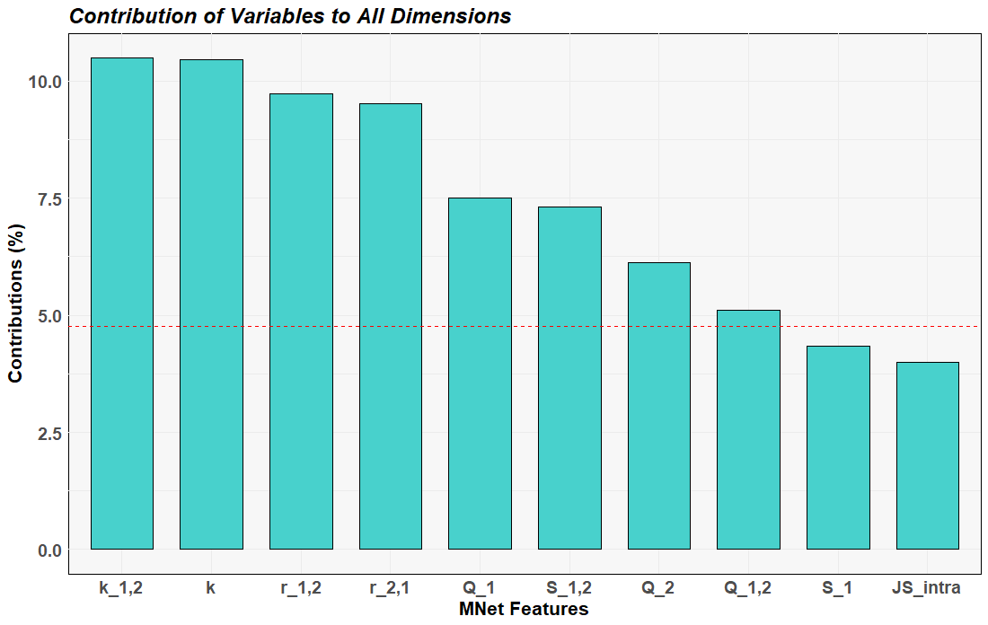
?figurename? 15: Bar plot with contributions of MNet features to the total of all 20 principal components formed by the PCA. The red dashed line on the plot indicates the expected average contribution.