Effects of Spatiotemporal Upscaling on Predictions of Reactive Transport in Porous Media

Abstract

The typical temporal resolution used in modern simulations significantly exceeds characteristic time scales at which the system is driven. This is especially so when systems are simulated overultra-long time-scales that are much longer than the typical temporal scales of forcing factors. We investigate the impact of space-time upscaling on reactive transport in porous media driven by time-dependent boundary conditions whose frequency characteristic time scale is much larger smaller than the characteristic time scale that at which transport is studied or observed at the macroscopic level. The focus is on transport of a reactive solute undergoing diffusion, advection and heterogeneous reaction on the solid grains boundaries. We first introduce a concept of spatiotemporal upscaling in the context of homogenization by multiple-scale expansions, and demonstrate the impact of time-dependent forcings and boundary conditions on macroscopic reactive transport. We then derive the macroscopic equation as well as the corresponding applicability conditions based on the order of magnitude of the Péclet and Damköhler dimensionless numbers. Finally, we demonstrate that the dynamics at the continuum scale is strongly influenced by the interplay between signal frequency at the boundary and transport processes at the pore level.

<>

Department of Energy Resources Engineering, Stanford University, Stanford, CA, USA

Farzaneh Rajabifrajabi@stanford.edu

Introduction of the concept of spatiotemporal upscaling in the context of homogenization by multiple-scale expansions.

Impact of time-dependent forcings and boundary conditions on macroscopic reactive transport in porous media.

The dynamics at the continuum scale is strongly influenced by the interplay between signal frequency at the boundary and transport processes at the pore level.

1 Introduction

Despite significant progress, accurate quantitative predictions of subsurface transport of highly reactive fluids remains a formidable challenge. Current numerical models suffer from significant predictive uncertainty, which undermines our ability to estimate future impact of, and the risks associated with, anthropogenic stressors on the environment. That is because subsurface flow and transport take place in complex highly hierarchical heterogeneous environments, and exhibit nonlinear dynamics and often lack spatiotemporal scale separation. The choice of an appropriate level of hydrogeologic model complexity continues to be a challenge. That is because subsurface flow and transport take place in complex highly hierarchical heterogeneous environments, and exhibit nonlinear dynamics and often lack spatiotemporal scale separation (Tartakovsky, 2013). The constant tension between fundamental understanding and predictive science on the one hand, and the need to provide science-informed engineering-based solutions to practitioners, on the other, is part of an ongoing debate on the role of hydrologic models (e.g. Miller et al., 2013). A physics-based model development follows a bottom-up approach which, through rigorous upscaling techniques, allows one to construct effective medium representations of fine-scale processes with different degrees of coupling and complexity (e.g. Wood and Valdes-Parada, 2013; Helming et al., 2013). Yet, current model deployment is generally based on established engineering practices and often relies on ‘simpler’ classical single-point closure local continuum descriptions with limited predictive capabilities.

The development of multiscale, multiphysics models aims at filling this scale gap and at addressing the limited applicability of classical local macroscopic models (Auriault, 1991; Auriault and Adler, 1995; Mikelic et al., 2006). Originated in the physics literature, multiscale methods were developed to couple particle to continuum solvers (Wadsworth and Erwin, 1990; Hadjiconstantinou and Patera, 1997; Abraham et al., 1998; Tiwari and Klar, 1998; Shenoy et al., 1999; Flekkoy et al., 2000; Alexander et al., 2002, 2005). Multiphysics domain-decomposition approaches (Peszyńska et al., 2002; Arbogast et al., 2007; Ganis et al., 2014), combined with multiscale concepts, led to the development of multiphysics, multiscale capabilities to address the multiscale nature of transport in the subsurface (Tartakovsky et al., 2008; Mehmani et al., 2012; Roubinet and Tartakovsky, 2013; Bogers et al., 2013; Mehmani and Balhoff, 2014; Yousefzadeh, 2020; Taverniers and Tartakovsky, 2017). The proposed methods predominantly focus on tackling partial or total lack of scale separation due to spatial heterogeneity, and are often based on spatial upscaling to construct coupling conditions between representations at different scales.

Upscaling methods enable one to formally establish a link between fine-scale (e.g. pore-scale) and observation-scale/macroscopic processes. Spatial upscaling methods include volume averaging averaging (e.g., Wood et al., 2003; Wood, 2009; Whitaker, 1999; Wood and Valdes-Parada, 2013) and its modifications and thermodynamically constrained averaging theory (Gray and Miller, 2005, 2014), the method of moments (Taylor, 1953; Brenner, 1980; Shapiro and Brenner, 1988), homogenization via multiple-scale expansions (Bensoussan et al., 1978; Hornung et al., 1994; Allaire et al., 2010; Hornung, 2012, e.g.,), and pore network models (Acharya et al., 2005). Cushman et al. (2002) provides a review of different upscaling methods. Comparative studies discuss differences and similarities of various upscaling techniques (e.g., Davit et al., 2013). Other upscaling approaches are described in (Brenner, 1987).

Yet, the need for computationally efficient ‘ultralong’ time predictions of subsurface system response to unsteady, and potentially highly fluctuating, forcing factors calls for the formulation of spatiotemporally-upscaled models. The practical need of averaging in time (as well as in space) originates from the disparity in temporal scales between the frequency at which the system is driven and the temporal horizon in which predictions are made, e.g., local micro-climate (precipitation, etc.) and the temporal scale relevant for climate studies, or local human activity and CO₂ sequestration scenarios, which, will be referred to as ‘long times’ in the following. In an attempt to curb computational burden, this problem is often tackled by adopting larger time-stepping and by temporally averaging time-dependent boundary conditions or driving forces (Beese and Wierenga, 1980; Wang et al., 2009; Yin et al., 2015).

While standard in the theory of turbulence (Taylor, 1959; Pope, 2000), time-averaging of fine-scale models of flow in porous media and geologic formations has attracted much less attention compared to its overbearing spatial-averaging sibling (He and Sykes, 1996; Pavliotis and Kramer, 2002; Rajabi and Battiato, 2015, 2017; Rajabi, 2021). Yet, the implications of temporally unresolved boundary conditions and driving forces in nonlinear subsurface systems appear to be dire: for example, Wang et al. (Wang et al., 2009) demonstrated showed that predictions of nonlinear transport in the vadose zone are greatly affected by the time resolution of forcing factors (e.g. annual versus hourly meteorological data). In partially saturated flows, Bresler and Dagan (1982) and Russo et al. (1989) found breakthrough curves under time-varying and time-averaged boundary conditions to be very different, with contaminant travelling faster and further in the former case. Similar highly dynamical conditions can be found in the subsurface interaction zone (SIZ) of riverine systems where environmental transitions often result in biogeochemical hotspots and moments that drive microbial activity and control organic carbon cycling (Stegen et al., 2016). To the best of our knowledge, with a few exceptions (Beese and Wierenga, 1980; He and Sykes, 1996; Pavliotis and Kramer, 2002; Wang et al., 2009), the effects of temporal averaging on macroscopic transport have been overlooked have not been thoroughly investigated. On the contrary, the impact of temporally fluctuating flows, boundary conditions and forcings in the context of upscaled transport in porous media has been the object of a number of studies. The seminal work by Smith (1981, 1982) investigated the impact of dispersion in oscillatory flows and derived a spatially upscaled delay-diffusion equation which accounts for memory effects. The effect of periodic oscillations leads to dynamic effective dispersion and time-dependent closure problems as analyzed by a number of authors (e.g. Moyne, 1997; Valdes-Parada and Alvarez Ramirez, 2011; Davit and Quintard, 2012; Valdes-Parada and Alvarez Ramirez, 2012; Dentz and Carrera, 2003; Pool et al., 2014, 2015, 2016; Nissan et al., 2017). Other studies primarily focused on spatial upscaling of transport in porous media with fluctuating flows and with changing pore-scale geometry due, e.g., to precipitation/dissolution processes (van Noorden et al., 2010; Kumar et al., 2011, 2014; Bringedal et al., 2016). In the context of atmospheric and oceanic pollutant transport where large-scale mean flow interacts non-linearly with small-scale fluctuations, Pavliotis et al. (Pavliotis, 2002; Pavliotis and Kramer, 2002; Pavliotis and Stuart, 2008) use higher-order homogenization to derive a rigorous homogenized equation and screen the temporal distribution of macroscopic quantities over long times by selecting appropriate spatial-temporally invariant volumes of the domain over which space-time volume averaging is applied. Fish and Chen (2004) presents a model for wave propagation in heterogeneous media by introducing multiple space-time scales with higher order homogenization theory to resolve stability and consistency issues.

Here, we are primarily interested in studying the effect of space-time averaging on the final form of the upscaled equations for long times (rather than early and/or pre-asymptotyc times (Valdes-Parada and Alvarez Ramirez, 2012)), i.e. when the influence on the initial condition has been forgotten, and their corresponding regimes of validity. This knowledge is important to assess the accuracy of, e.g., numerical models wherein the temporal numerical resolution significantly exceeds characteristic scales at which the system is driven. HereSpecifically, we focus on reactive transport in undeformable porous media driven by time-varying boundary conditions, whose frequency is much larger than the characteristic time scale at which transport is studied or observed at the macroscopic scale. A typical temporal resolution used in modern simulations significantly exceeds characteristic scales at which the system is driven. Some of the questions we are interested in addressing are: under which conditions (e.g. signal frequency) the instantaneous macroscopic response of the system can be decoupled from temporally fluctuating forcing factors (e.g. temporally dependent injection rates at the boundary)? How to properly account for time-averaged boundary conditions in upscaled models? We propose to address these questions by introducing the concept of spatiotemporal upscaling in the context of asymptotic multiple scale expansions. The main contribution of the paper is to explicitly address the question of whether or not, and how, space-time upscaling affects reactive transport modeling, and more importantly, if/what conditions of applicability of upscaled equations need to be satisfied for the macroscopic models to be accurate. This problem becomes of increasing importance as hydrologic modeling (and its relation to climate models) expands the time-window (from months to years to decades and more) used for forward predictions, while the time resolution in our simulations remains constrained by computational costs.

The manuscript is organized as follows. In Section 2, we present the pore-scale model describing advective and diffusive transport of a solute subject to time-dependent Dirichlet conditions at the macroscale boundary and undergoing a heterogenous chemical reaction with the solid matrix. In Section 3, we introduce the concept of spatiotemporal upscaling in the context of homogenization by multiple-scale expansions, and demonstrate the impact of time-dependent forcings and boundary conditions on macroscopic reactive transport. We first classify the macroscopic dynamics in three regimes (slowly, moderately and highly fluctuating regimes) and then derive a set of frequency-dependent conditions under which scales are separable. Section 4 provides a physical interpretation of the key analytical results of Section 3. In Section 5, we discuss different transport regimes in terms of relevant dimensionless numbers. Conclusions and outlook are given in Section 6.

2 Problem Formulation

2.1 Domain and governing equations

Let $\hat{\Omega}$ be a domain in $\mathcal{R}^{n}$ ($n\geq 2$), bounded by $\partial\hat{\Omega}$, of characteristic length $L$ such that $\hat{\Omega}=\hat{\Omega}_{s}\cup\hat{\Omega}_{p}$, where $\hat{\Omega}_{s}$ and $\hat{\Omega}_{p}$ are the solid and pore phases in $\hat{\Omega}$, respectively, and $\hat{\Omega}_{p}$ is fully saturated with a viscous fluid. The boundary between the solid and the pore space domains is $\hat{\Gamma}$. The domain $\hat{\Omega}$ is composed of repeating unit cells $\hat{Y}=\hat{\mathcal{B}}\cup\hat{\mathcal{G}}$ of characteristic size $l$ with $l\ll L$, where $\hat{\mathcal{G}}$ and $\hat{\mathcal{B}}$ are the solid and pore phases in $\hat{Y}$, respectively. The geometric scaling parameter

$$\varepsilon:=\dfrac{l}{L}\ll 1$$ (1)

relates the size of the pore-scale unit cell to the corresponding macroscale (or observation spatial scale).

The laminar incompressible flow of a viscous fluid through the pore space $\hat{\Omega}_{p}$ satisfies Stokes law and the continuity equation

$${\mu}{\hat{\nabla}}^{2}\hat{\mathbf{v}}_{\varepsilon}-{\hat{\nabla}}{\hat{p}_{\varepsilon}}=0,\quad\hat{\mathbf{x}}\in\hat{\Omega}^{\varepsilon}_{p},$$ (2a)

$$\hat{\nabla}\cdot\hat{\mathbf{v}}_{\varepsilon}=0,\quad\hat{\mathbf{x}}\in\hat{\Omega}^{\varepsilon}_{p},$$ (2b)

subject to

$$\hat{\mathbf{v}}_{\varepsilon}=0,\quad\mathbf{x}\in{\hat{\Gamma}}^{\varepsilon},$$ (3)

and appropriate boundary conditions on $\mathbf{v}_{\varepsilon}$ and $\hat{p}_{\varepsilon}$ on the domain boundary $\partial\hat{\Omega}$. In (2) and (3), where $\hat{\mathbf{v}}_{\varepsilon}$ [LT^-1], $\hat{p}_{\varepsilon}$ and $\mu$ are the fluid velocity, dynamic pressure and dynamic viscosity, respectively. The transport of a reactive solute $\mathcal{M}$, dissolved in the fluid, with molar concentration $\hat{c}_{\varepsilon}(\hat{\mathbf{x}},\hat{t})$ [molL^-3] at $\hat{\mathbf{x}}\in\hat{\Omega}^{\varepsilon}_{p}$ and time $\hat{t}>0$, is governed by

$$\dfrac{\partial{\hat{c}}_{\varepsilon}}{\partial{\hat{t}}}+\hat{\mathbf{v}}_{\varepsilon}\cdot{\hat{\nabla}}\hat{c}_{\varepsilon}={\hat{\nabla}}\cdot(\hat{\textbf{D}}{\hat{\nabla}}\hat{c}_{\varepsilon}),\quad\hat{\mathbf{x}}\in{\hat{\Omega}}^{\varepsilon}_{p},\quad\hat{t}>0$$ (4)

where $\hat{\mathbf{D}}$ [L²T^-1] is the molecular diffusion tensor, $[\mathbf{D}\nabla c_{\varepsilon}]_{i}=D_{ij}\partial_{x_{j}}c_{\varepsilon}$ is a matrix-vector multiplication, and ‘$\cdot$’ represents a scalar product, e.g. $\hat{\mathbf{v}}_{\varepsilon}\cdot{\hat{\nabla}}\hat{c}_{\varepsilon}=\hat{v}_{\varepsilon,i}\partial_{x_{i}}c_{\varepsilon}$, where summation is implied over a repeated index. The nonlinear heterogenous precipitation/dissolution reaction of solute $\mathcal{M}$ at the solid grains boundary can be modelled through the following boundary condition on $\Gamma$

$$-\mathbf{n}\cdot{\hat{\textbf{D}}}{\hat{\nabla}}{\hat{c}}_{\varepsilon}={\hat{k}}({\hat{c}}^{a}_{\varepsilon}-\overline{c}^{a})\qquad\hat{\mathbf{x}}\in{\Gamma}^{\varepsilon}$$ (5)

which represents a mass balance across the solid-liquid interface. Equation (4) is subject to initial conditions

$$\hat{c}_{\varepsilon}(\hat{\mathbf{x}},0)=\hat{c}_{\mbox{\tiny{in}}}(\hat{\mathbf{x}}),\quad\hat{\mathbf{x}}\in\hat{\Omega}_{p}$$ (6)

and boundary conditions on $\partial\hat{\Omega}=\partial\hat{\Omega}_{D}\cup\partial\hat{\Omega}_{N}\cup\partial\hat{\Omega}_{R}$, where $\partial\hat{\Omega}_{i}$, $i=\{D,N,R\}$ represent a portion of the boundary subject to Dirichlet, Neumann or Robin boundary conditions, respectively. Without loss of generality, we assume $\partial\hat{\Omega}_{D}$ is subject to time-varying boundary conditions, i.e.

$$\hat{c}_{\varepsilon}(\hat{\mathbf{x}}_{D},\hat{t})=\hat{c}_{D}(\hat{t}).$$ (7)

where $\hat{\tau}$ is the characteristic time scale of the boundary forcing The previous boundary condition models a spatially localized seasonal release of reacting solute (e.g. contaminant or nutrient), associated to, e.g., respiration processes of bacteria, hydrologic cycles that create local chemical hotspots (e.g. in the hyporheic corridor), etc. We emphasize that other time-dependent boundary conditions could be used in place of (15), e.g. Danckwerts’ (Danckwerts, 1953).

2.2 Dimensionless formulation

We define the following dimensionless quantities

$$c=\dfrac{{\hat{c}}_{\varepsilon}}{\hat{c}_{\mbox{\tiny{in}}}},\quad\textbf{D}=\dfrac{{\hat{\mathbf{D}}}}{D},\quad\mathbf{x}=\dfrac{{\hat{\mathbf{x}}}}{L},\quad\mathbf{v}_{\varepsilon}=\dfrac{\hat{\mathbf{v}}_{\varepsilon}}{U},\quad t=\dfrac{{\hat{t}}}{\tau_{c}},\quad p=\dfrac{{\hat{p}}l^{2}}{{\nu}UL}$$ (8)

where $U$, $D$ and $\tau_{c}$ are characteristic scales for velocity, diffusivity and time. We set $\tau_{c}$ as the diffusive time-scale, i.e.

$$\tau_{c}=\dfrac{L^{2}}{D},$$ (9)

Inserting (8) and (9) in (2)-(15), one obtains

$$\varepsilon^{2}\nabla^{2}\mathbf{v}_{\varepsilon}-\nabla p_{\varepsilon}=0\quad\mbox{and}\quad\nabla\cdot\mathbf{v}_{\varepsilon}=0,\quad\mathbf{x}\in{\Omega}^{\varepsilon}_{p}$$ (10)

subject to

$$\mathbf{v}_{\varepsilon}=0,\quad\mathbf{x}\in\Gamma^{\varepsilon},$$ (11)

and

$$\dfrac{\partial c_{\varepsilon}}{\partial t}+\nabla\cdot(-\textbf{D}\nabla c_{\varepsilon}+\mbox{Pe}\mathbf{v}_{\varepsilon}c_{\varepsilon})=0,\quad\mathbf{x}\in{\Omega}^{\varepsilon}_{p},\quad t>0$$ (12)

subject to

$$-\mathbf{n}\cdot\textbf{D}\nabla c_{\varepsilon} =\mbox{Da}(c^{a}_{\varepsilon}-1)\qquad\mathbf{x}\in\Gamma^{\varepsilon},\quad t>0$$ (13)

$$c(\mathbf{x},0) =c_{\mbox{\tiny{in}}}(\mathbf{x})\qquad\mathbf{x}\in\Omega_{p}^{\varepsilon},$$ (14)

and to time-varying Dirichlet boundary conditions on a subset of the macroscopic boundary $\partial\Omega_{D}$, i.e.

$$c_{\varepsilon}(\mathbf{x}_{D},t)=c_{D}(t).$$ (15)

In (12) and (13)

$$\mbox{Pe}:=\dfrac{\tau_{d}}{\tau_{a}}=\dfrac{UL}{D},\qquad\text{and}\qquad\mbox{Da}:=\dfrac{\tau_{d}}{\tau_{r}}=\dfrac{L\hat{k}\hat{c}^{a-1}_{0}}{D},$$ (16)

are the Péclet and Damkhöler numbers, defined as the ratio between the diffusive time $\tau_{d}$ and the advection and reaction time scales, $\tau_{a}$ and $\tau_{r}$, respectively, with $\tau_{a}=L/U$ and $\tau_{r}=L/(\hat{k}\hat{c}_{0}^{a-1})$.

3 Space-Time Homogenization via Multiple-Scale Expansions

In this section, we generalize the multiple-scale expansion method to upscale in both space and time the pore scale dimensionless equations (10) and (12) to the macroscale, and to derive effective equations for the space-time averages of the flow velocity $\langle\mathbf{v}_{\varepsilon}\rangle$ and the solute concentration $\langle c_{\varepsilon}\rangle$ while accounting for time-varying boundary conditions. We emphasize a similar approach can be employed to handle time-varying source terms and coefficients.

3.1 Preliminaries and Extensions to Time Homogenization

Within the multiple-scale expansion framework, we introduce a ‘fast’ space variable $\mathbf{y}$ defined in the unit cell $Y$, i.e. $\mathbf{y}\in Y$. Furthermore, if the system is driven by time-varying boundary conditions or forcing factors with characteristic time scale $\hat{\tau}\ll T$ where $T$ is the observation time scale, one can define a temporal scaling parameter

$$\omega:=\dfrac{\hat{\tau}}{T}\ll 1,$$ (17)

that relates the driving force/boundary condition frequency ($\sim 1/\hat{\tau}$) and the observation (macroscopic) time scale $T$. We define the exponent $\gamma$ such that

$$\varepsilon=\omega^{\gamma},$$ (18)

i.e. $\gamma$ quantifies the separation between temporal and spatial scales and is uniquely determined once the characteristic length and time scales of the problem are identified. Each variable is defined as follows,

$$\mathbf{y}=\varepsilon^{-1}\mathbf{x},\quad\mbox{and}\quad\tau=\omega^{-1}t.$$ (19)

For any pore-scale quantity $\psi_{\varepsilon}$,

$$\langle\psi_{\varepsilon}\rangle_{Y}\equiv\frac{1}{|Y|}\int\limits_{\mathcal{B}(\mathbf{x})}\psi_{\varepsilon}\mathrm{d}\mathbf{y},\quad\langle\psi_{\varepsilon}\rangle_{\mathcal{B}}\equiv\frac{1}{|\mathcal{B}|}\int\limits_{\mathcal{B}(\mathbf{x})}\psi_{\varepsilon}\mathrm{d}\mathbf{y},\,\mbox{and}\,\,\langle\psi_{\varepsilon}\rangle_{\Gamma}\equiv\frac{1}{|\Gamma|}\int\limits_{\Gamma(\mathbf{x})}\psi_{\varepsilon}\mathrm{d}\mathbf{y}$$ (20)

are three local spatial averages (function of $\mathbf{x}$) over the pore space $\mathcal{B}(\textbf{x})$ of the unit cell $Y(\textbf{x})$ centered at x. In (20), $\langle\psi_{\varepsilon}\rangle_{Y}=\phi\langle\psi_{\varepsilon}\rangle_{\mathcal{B}}$ and $\phi=|\mathcal{B}|/|Y|$ is the porosity. Similarly, one can define temporal averages (function of $t$) over a time unit cell $\mathcal{I}$ centered at $t$, i.e,

$$\langle\psi_{\varepsilon}\rangle_{\mathcal{I}}\equiv\frac{1}{|\mathcal{I}|}\int\limits_{\mathcal{I}(t)}\psi_{\varepsilon}\mathrm{d}\tau.$$ (21)

where $\mathcal{I}$ is the smallest time-scale resolved at the macroscale, e.g. the discretization time-step at the continuum scale. The space-time averages $\langle\psi_{\varepsilon}\rangle_{\mathcal{IB}}$ and $\langle\psi_{\varepsilon}\rangle$ are is defined as

$$\langle\psi_{\varepsilon}\rangle_{\mathcal{IB}}:=\langle\langle\psi_{\varepsilon}\rangle_{\mathcal{I}}\rangle_{\mathcal{B}}=\langle\langle\psi_{\varepsilon}\rangle_{\mathcal{B}}\rangle_{\mathcal{I}}.$$ (22)

and

$$\langle\psi_{\varepsilon}\rangle:=\langle\langle\psi_{\varepsilon}\rangle_{\mathcal{I}}\rangle_{Y}=\langle\langle\psi_{\varepsilon}\rangle_{Y}\rangle_{\mathcal{I}}=\phi\langle\psi_{\varepsilon}\rangle_{\mathcal{IB}}.$$ (23)

Furthermore, any pore-scale function $\psi_{\varepsilon}(\mathbf{x},t)$ can be represented as $\psi_{\omega}(\mathbf{x},t)$ through (18) and $\psi_{\omega}\left(\mathbf{x},t\right):=\psi(\mathbf{x},\mathbf{y},t,\tau)$. Replacing $\psi_{\omega}\left(\mathbf{x},t\right)$ with $\psi(\mathbf{x},\mathbf{y},t,\tau_{\mathrm{a}},\boldsymbol{\tau}_{\mathrm{r}})$ gives the following relations for the spatial and temporal derivatives,

$$\nabla\psi_{\omega}=\nabla_{\mathbf{x}}\psi+\varepsilon^{-1}\nabla_{\mathbf{y}}\psi=\nabla_{\mathbf{x}}\psi+\omega^{-\gamma}\nabla_{\mathbf{y}}\psi,\quad\mbox{and}\quad\dfrac{\partial\psi_{\omega}}{\partial t}=\dfrac{\partial\psi}{\partial t}+\omega^{-1}\dfrac{\partial\psi}{\partial\tau}$$ (24)

respectively. The function $\psi$ is represented as an asymptotic series in powers of $\omega$,

$$\psi(\mathbf{x},\mathbf{y},t,\tau)=\sum_{m=0}^{\infty}\omega^{m}\psi_{m}(\mathbf{x},\mathbf{y},t,\tau),$$ (25)

wherein $\psi_{m}(\mathbf{x},\mathbf{y},t,\tau)$, $m=0,1,\ldots$, are $Y$-periodic in $\mathbf{y}$. Finally, we set

$$\mbox{Pe}=\omega^{-\alpha},\quad\mbox{and}\quad\mbox{Da}=\omega^{\beta},$$ (26)

with the exponents $\alpha$ and $\beta$ determining the system behavior. We seek the asymptotic space-time average behavior of $\psi_{\omega}$ as $\omega\rightarrow 0$ for any arbitrary time-scale separation parameter $\gamma$.
It should be emphasized that, an important step in solving the cascade of equations for $\psi_{0},\psi_{1},\cdot\cdot\cdot$, is consistently checking whether the solvability condition is satisfied. Otherwise, the derivation leads to misleading results. More specifically, when seeking a solution for $\psi_{1}$, we have to impose the solvability condition. This condition ensures existence and uniqueness of a solution rigorously by employing the Fredholm Alternative. Critical points to consider while employing the homogenization theory to upscale the transport equation are summarized by Auriault (2019), where the author explicitly mentions that the averaging process is imposed by Fredholm Alternative, and there is no arbitrary step along the derivation process.

3.2 Upscaled Transport Equations and Homogenizability Conditions

The homogenization of the Stokes equations (2) leads to the classical result

$$\langle\mathbf{v}\rangle=-\mathbf{K}\cdot\nabla P_{0},\qquad\nabla\cdot\langle\mathbf{v}\rangle=0,\quad\mathbf{x}\in\Omega,$$ (27)

where the dimensionless permeability tensor $\mathbf{K}$ is defined as $\mathbf{K}=\langle\mathbf{k}\rangle$ and $\mathbf{k}$ is the closure variable, solution of the closure problem

$$\nabla^{2}\textbf{k}+\mathbf{I}-\nabla\textbf{a}=0,\qquad\nabla\cdot\mathbf{k}=0,\qquad\textbf{y}\in\mathcal{B}$$ (28)

subject to $\mathbf{k}(\textbf{y})=0$ for $\textbf{y}\in\Gamma$ and $\langle\textbf{a}\rangle=0$, where $\mathbf{a}$ is $Y$-periodic (Hornung, 2012, pp. 46-47, Theorem 1.1).

Here, we are interested in studying the system for long times, also referred to as ‘quasi-steady stage’ (as per definition of Valdes-Parada and Alvarez Ramirez (2012)), i.e. when both time- and length-scales can be separated. Thenas detailed in Appendix A, the space-time homogenization of the pore-scale reactive transport equations (12)-(15) up to order $\omega^{2}$, leads to (Rajabi, 2021) (details in Appendix A)

$$\phi\dfrac{\partial\langle c\rangle_{\mathcal{IB}}}{\partial t}=\nabla\cdot\left[\tilde{\tilde{\textbf{D}}}^{\star}\nabla\langle c\rangle_{\mathcal{IB}}-\mbox{Pe}\langle c\rangle_{\mathcal{IB}}\langle\mathbf{v}\rangle_{\mathcal{IB}}\right]+\phi\omega^{-\gamma}\mathcal{K}^{\star}\mbox{Da}(1-\langle c\rangle_{\mathcal{IB}}^{a}),$$

$$(\mathbf{x},t)\in\Omega\times(0,T),$$ (29)

where the effective coefficients $\mathcal{K^{\star}}$, and $\tilde{\tilde{\textbf{D}}}^{\star}$ are defined as

$$\mathcal{K^{\star}} =\dfrac{|\varGamma|}{|\mathcal{B}|},$$ (30)

$$\tilde{\tilde{\textbf{D}}}^{\star} =\langle\textbf{D}(\mathbf{I}+\omega^{1-\gamma}\nabla_{\mathbf{y}}\boldsymbol{\chi})\rangle+\omega^{1-\alpha}\langle\boldsymbol{\chi}\mathbf{k}\rangle\cdot\nabla_{\mathbf{x}}P_{0},$$ (31)

and $\boldsymbol{\chi}(\mathbf{y},\tau)$ and $\lambda(\mathbf{y},\tau)$ are is the closure variable. The effective coefficient $\tilde{\textbf{D}}^{\star}$ and $\tilde{\textbf{D}}^{\prime}$ are is computed through the solution of two the unsteady auxiliary cell problem for $\lambda(\mathbf{y},\tau)$ and $\boldsymbol{\chi}(\mathbf{y},\tau)$, i.e.

$$\dfrac{\partial\boldsymbol{\chi}}{\partial\tau}+\omega^{-\alpha}(\mathbf{v}_{0}-\langle\mathbf{v}_{0}\rangle_{\mathcal{I}\mathcal{B}})-\omega^{-\gamma}\nabla_{\mathbf{y}}\cdot\textbf{D}(\mathbf{I}+\omega^{1-\gamma}\nabla_{\mathbf{y}}\boldsymbol{\chi})+\omega^{1-\gamma-\alpha}\mathbf{v}_{0}\cdot(\nabla_{\mathbf{y}}\boldsymbol{\chi})=0,\quad\mathbf{y}\in\mathcal{B},$$

$$\mathbf{n}\cdot\textbf{D}(\mathbf{I}+\omega^{1-\gamma}\nabla_{\mathbf{y}}\boldsymbol{\chi})=0,\quad\mathbf{y}\in\mathcal{B},$$ (32)

$$\boldsymbol{\chi}(\mathbf{y},0)=\boldsymbol{\chi}_{\mbox{\tiny{in}}}(\mathbf{y}),$$

and $\langle\boldsymbol{\chi}\rangle_{\mathcal{B}}=0$, where $\mathbf{v}_{0}=-\mathbf{k}(\mathbf{y})\cdot\nabla_{\mathbf{x}}P_{0}$ is the solution of the homogenized flow equation (27), provided the following conditions are met (Rajabi, 2021)

1. $\varepsilon\ll 1$,

2. $\omega\ll 1$,

3. $\langle\boldsymbol{\chi}\rangle_{\mathcal{I}\Gamma}\approx\langle\boldsymbol{\chi}\rangle_{\mathcal{IB}}$,

4. $\langle\lambda\rangle_{\Gamma}\approx\langle\lambda\rangle_{\mathcal{B}}$,

Additional bounds on the Damköhler and Péclet numbers must be satisfied depending on the time-space scale separation parameter $\gamma$. Specifically,

1. when $\varepsilon<\omega$, i.e. $\gamma>1$, the system is referred to as slowly fluctuating and the additional conditions to guarantee that scale separation occurs are

   1. $\mbox{Pe}<\omega^{-1}$

   2. $\mbox{Da}/\mbox{Pe}<\varepsilon$

   3. $\mbox{Da}<\varepsilon$.

2. When $\omega<\varepsilon<\omega^{1/2}$ (or $\omega\approx\varepsilon$), i.e. $1/2<\gamma<1$, the system is referred to as moderately fluctuating and the additional conditions to guarantee that scale separation occurs are

   1. $\dfrac{\varepsilon}{\omega}<\mbox{Pe}<\omega^{-1}$

   2. $\mbox{Da}/\mbox{Pe}<\omega$.

3. When $\omega^{1/2}<\varepsilon<1$ (or $\varepsilon\gg\omega$), i.e. $0<\gamma<1/2$, the system is referred to as highly fluctuating and the additional conditions to guarantee that scale separation occurs are

   1. $\mbox{Pe}<\omega^{-1}$

   2. $\mbox{Da}/\mbox{Pe}<\omega$

   3. $\mbox{Da}<\omega/\varepsilon$.

These conditions can be graphically visualized in a phase diagram in the $(\mathrm{Pe},\mathrm{Da})$-space, or the $(\alpha,\beta)$-space for the three different regimes (Rajabi, 2021). The bounds for slowly fluctuating systems (i.e. $\varepsilon<\omega$, i.e. $\gamma>1$) are summarized in the $(\alpha,\beta)$-plane of Figure 1(a), where the lines $\beta=\gamma$, $\alpha+\beta=\gamma$ and $\alpha=1$ correspond to $\mbox{Da}=\varepsilon$, $\mbox{Da}/\mbox{Pe}=\varepsilon$ and $\mbox{Pe}=\omega^{-1}$, respectively. For moderately fluctuating systems where $\omega\approx\varepsilon$, the bounds are summarized in the $(\alpha,\beta)$-plane of Figure 1(b). The lines $\alpha+\beta=1$, $\alpha=1$ and $\alpha=1-\gamma$ correspond to $\mbox{Da}/\mbox{Pe}=\omega$, $\mbox{Pe}=\omega^{-1}$ and $\mbox{Pe}=\varepsilon/\omega$, respectively. Finally, in highly fluctuating systems, i.e. when $\omega^{1/2}<\varepsilon<1$ (or $\varepsilon\gg\omega$), the previous conditions are summarized in Figure 1(c), where the line $\beta=1-\gamma$ corresponds to $\mbox{Da}=\omega/\varepsilon$. Figure 1(d) overlaps the applicability conditions for the three regimes to allow direct comparison. We emphasize that, while Eq. (29) has the form of a classical advection-reaction-dispersion equation, both the (i) the form of its effective coefficients and (ii) the conditions under which both spatial and temporal scales are fully decoupled explicitly depend on $\gamma$, i.e. the scale parameter that relates spatial scales and the frequency of the boundary fluctuations. Furthermore, Eq. (29) is consistent with the results obtained through space and time volume averaging (ST-averaging) by He and Sykes (1996) where, for a homogeneous distribution of elementary (space-time averaging) domains, the ST-upscaling using volume averaging degenerates into a classical volume average.

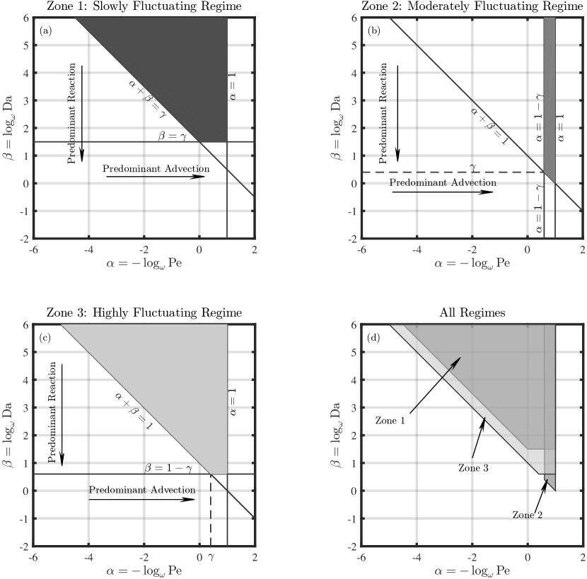
Figure 1: Applicability conditions in the $(\alpha,\beta)$-phase space for: (a) slowly fluctuating regimes (Zone 1), i.e. $\varepsilon<\omega$ or $\gamma>1$; (b) moderately fluctuating regimes (Zone 2), i.e. $\omega<\varepsilon<\omega^{1/2}$ ($\omega\approx\varepsilon$) or $1/2<\gamma<1$; (c) highly fluctuating regimes (Zone 3), i.e. $\omega^{1/2}<\varepsilon<1$ ($\varepsilon\gg\omega$) or $0<\gamma<1/2$; (d) all regimes overlapped for direct comparison. In each Figure, the shaded region identifies sufficient conditions for the validity of macroscopic equation in terms of Da and Pe numbers. In the white region, scales are not well separated and macroscopic and microscopic models should be solved simultaneously.

4 Discussion and Physical Interpretation

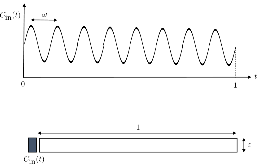
Figure 2: Time-dependent solute injection boundary condition $(C_{\mbox{in}})$ (top) at the inlet of a planar thin impermeable fracture of aperture $\varepsilon\ll 1$ (bottom). The time-varying boundary condition has a frequency of $\omega^{-1}$ (or characteristic dimensionless time scale/period $\omega\ll 1$). Figure not in scale.

In this Section, we are concerned with providing a physical interpretation of the (formally derived) thresholds on $\gamma$ and their connection with the regimes classification (slowly, moderately and highly fluctuating regimes) proposed in the previous Section. For this purpose, we consider a conceptual example, which, despite its simplicity, maintains enough complexity to provide useful physical insights on the theoretical results. Without loss of generality, let us consider a pressure-driven flow through a thin bidimensional channel of length $L$ and aperture $l$ with $l\ll L$. For a channel of width $l$, the length $L$ is to be interpreted as the “observation scale”. Steady state fully-developed incompressible flow is assumed. Reactive solute transport at the pore-scale is governed by (4) subject to (5) on the fracture walls. Time varying Dirichlet boundary conditions for solute concentration are imposed at the fracture inlet. The characteristic time scale of the fluctuating boundary conditions is $\hat{\tau}\ll T$, with $T$ the macroscale observation time. Figure 2 shows a sketch of the system. As discussed in Section 3.1, the space and time scale separation parameters are

$$\varepsilon\equiv{\dfrac{l}{L}}\ll 1,\quad\mbox{and}\quad\omega\equiv\dfrac{{\hat{\tau}}}{T}\ll 1.$$ (33)

The (dimensional) time scales for diffusive and advective transport at the macro-and micro-scale are

$$\hat{t}_{\tiny{\mbox{d,macro}}}=\dfrac{L^{2}}{D},\quad\hat{t}_{\tiny{\mbox{a,macro}}}=\dfrac{L}{U},$$ (34a)

$$\hat{t}_{\tiny{\mbox{d,micro}}}=\dfrac{l^{2}}{D},\quad\hat{t}_{\tiny{\mbox{a,micro}}}=\dfrac{l}{U},$$ (34b)

respectively, and the (macroscopic) Peclét number is defined as in (16)

$$\mbox{Pe}:=\dfrac{\hat{t}_{\tiny{\mbox{d,macro}}}}{\hat{t}_{\tiny{\mbox{a,macro}}}}=\dfrac{1}{\varepsilon}\dfrac{\hat{t}_{\tiny{\mbox{d,micro}}}}{\hat{t}_{\tiny{\mbox{a,micro}}}}=\dfrac{LU}{D}.$$ (35)

Using a diffusive scaling, i.e. $t:=\dfrac{\hat{t}}{\hat{t}_{\tiny{\mbox{d,macro}}}}$, the time scales defined in (34a) can be expressed in terms of powers of $\varepsilon$ or $\omega$

$${t}_{\tiny{\mbox{d,macro}}}=\omega^{0}=\varepsilon^{0},\qquad {t}_{\tiny{\mbox{d,micro}}}=\omega^{2\gamma}=\varepsilon^{2},$$ (36a)

$${t}_{\tiny{\mbox{a,macro}}}=\omega^{\alpha}=\varepsilon^{\alpha/\gamma},\qquad {t}_{\tiny{\mbox{a,micro}}}=\omega^{\alpha+\gamma}=\varepsilon^{1+\alpha/\gamma},$$ (36b)

Time scale	$\mathcal{O}(\omega)$	$\mathcal{O}(\varepsilon)$
BCs	$\omega^{1}$	$\varepsilon^{1}$
${t}_{\tiny{\mbox{d,macro}}}$	$\omega^{0}$	$\varepsilon^{0}$
${t}_{\tiny{\mbox{a,macro}}}$	$\omega^{\alpha}$	$\varepsilon^{\alpha/\gamma}$
${t}_{\tiny{\mbox{d,micro}}}$	$\omega^{2\gamma}$	$\varepsilon^{2}$
${t}_{\tiny{\mbox{a,micro}}}$	$\omega^{\alpha+\gamma}$	$\varepsilon^{1+\alpha/\gamma}$

Table 1: Summary of the characteristic time scales of transport processes at the micro- and macro-scale in terms of either integer powers of $\omega$ and $\varepsilon$.

(summarized in Table 1) and their relative magnitude is controlled by the exponents $\gamma$, $\alpha$ and $\beta$. Importantly, the characteristic diffusion time ${t}_{\tiny{\mbox{d,micro}}}$ scales as $\varepsilon^{2}$, i.e. the separation of scale parameter $\varepsilon$ can be related to the characteristic dimensionless time scale of the dominant mass transport mechanisms at the microscale. This observation allows us (i) to relate the dimensionless period of the oscillations $\omega$ to the dimensionless time-scale of mass transport processes at the pore scale (specifically, diffusion), and (ii) to elucidate the physical meaning of the $\gamma$-thresholds (i.e. $\gamma=1/2$ and $\gamma=1$) that identify the slowly, moderately and highly fluctuating regimes. Specifically, a slowly fluctuating regime corresponds to a system driven by time-dependent boundary conditions with a characteristic time-scale $\omega$ greater than $\varepsilon$, i.e. $\omega\gg{t}_{\tiny{\mbox{d,micro}}}$: in this regime, temporal fluctuations in the boundary conditions are very slow compared to pore-scale diffusion, and the dynamics at the microscale is exclusively controlled by local pore-scale mass transport processes. This translates in a steady state diffusive problem for the closure variables as discussed in Section 5.1. In the moderately fluctuating regime, $\omega<\varepsilon<\omega^{1/2}$ or, equivalently, $\omega^{2}<{t}_{\tiny{\mbox{d,micro}}}<\omega$, i.e. $\omega$ and ${t}_{\tiny{\mbox{d,micro}}}$ are of the same order of magnitude. While the local cell problems for the closure variables are still steady state (Section 5.2), advection and diffusion become the two mechanisms that guarantee mixing at the pore-scale. In the highly fluctuating regime, $\omega^{1/2}<\varepsilon<1$ or $\omega\ll{t}_{\tiny{\mbox{d,micro}}}$, i.e. the characteristic time scale at which the system is driven is much smaller than pore-scale diffusion time. In this regime spatial and temporal scales can still be separated, but the high frequency boundary conditions augment local mixing and the local cell problem becomes unsteady and advective and unsteady effects will control mass transport at the pore-scale (Section 5.3). It is worth noticing that the applicability domain in the (Da-Pe) space for the moderately fluctuating regimes is much smaller than those for both slowly and highly fluctuating case: contrary to intuition, a slower advection drags the system outside the homogenizability conditions in a moderately fluctuating regime. This can be explained as follows: when diffusion and advection are the dominant mechanisms controlling transport at the pore-scale, slower advection results in an increased longitudinal, rather than transversal, mixing, making the applicability conditions in terms of Pe number much more stringent. Surprisingly, the applicability conditions in the slowly fluctuating case are a subset of those for the highly fluctuating scenario, i.e. the latter has less stringent constraints in terms of both Pe and Da numbers for the same value of $\gamma$: we hypothesize that advection and unsteadiness (and their combination) may prove more effective in achieving pore-scale mixing, i.e. may contribute to an enhancement of mixing at the pore-scale. In presence of very fast fluctuations (at a time scale much smaller than diffusion), the pore-scale concentration in the fracture can be idealized as a periodic sequence of very thin strips of fixed concentration which travel downstream due to advection. As a result, while the system is very heterogeneous in the longitudinal direction (for times smaller than the characteristic diffusion time), it is well-mixed in the transverse direction, i.e. along the unit cell. This hypothesis is subject of current numerical investigations.

Importantly, according to (33), once the physical domain of interest is identified (i.e. $\varepsilon$ is fixed) and the characteristic time scale $\hat{\tau}$ of the boundary conditions determined, the macroscopic time horizon $T$ (i.e. the time at which predictions are ought to be made) uniquely defines $\omega$, and consequently, $\gamma$. This implies that, for a given pair (Pe, Da), the accuracy of the upscaled equation used for forward predictions can be greatly affected by modifying $T$: for example if $T_{2}>T_{1}$, then $\omega_{2}<\omega_{1}\ll 1$; for the same $\varepsilon$, this corresponds to $\gamma_{2}<\gamma_{1}$ since $\gamma:=\log\varepsilon/\log\omega$, i.e. the applicability conditions may change from a slowly to a moderately fluctuating regime. This observation suggests that caution should be employed when systems driven by time-varying boundary conditions/forcings are de facto, if not voluntarily, upscaled both in space and time, e.g. due to computational limitations.

In the following Section we quantitatively characterize the dominant transport mechanisms at the pore-and continuum-scale for different values of Da and Pe numbers.

Figure 3: (a) Slowly fluctuating regime: the time-varying boundary condition $C_{\tiny{\mbox{in}}}(t)$ has a characteristic time scale much larger than pore-scale diffusion, i.e. $\omega\gg{t}_{\tiny{\mbox{d,micro}}}$. (b) Moderately fluctuating regime: the characteristic time scale of the boundary condition $C_{\tiny{\mbox{in}}}(t)$ is of the same order of pore-scale diffusion, i.e. $\omega\approx{t}_{\tiny{\mbox{d,micro}}}$. (c) Highly fluctuating regime: pore-scale diffusion is much slower than the time scale imposed by $C_{\tiny{\mbox{in}}}(t)$. Figure not in scale.

5 Special Cases

In this Section, we investigate specific flow and transport regimes under which the upscaled equation (29) and the closure problem (3.2) can be simplified. Such transport regimes are identified by the order of magnitude of the Damköhler and Peclét numbers. Differently from similar analyses on the applicability conditions of diffusive-advective-reactive systems under steady boundary conditions (or forcings) (Auriault and Adler, 1995) and/or the dynamics of composite materials (Auriault, 1991), here we are specifically interested in elucidating the impact of boundary/forcing frequency on the form of the upscaled equations for the highly, moderately and slowly fluctuating regimes and any given pair of Damköhler and Peclét numbers satisfying the conditions outlined in Section 3.2. Our analysis below shows that for systems with the same Damköhler and Peclét numbers, the form of the space-time upscaled equations and of the closure problem depends on the frequency of the boundary condition, i.e. pore-scale mixing is controlled by the interplay of diffusion, advection and unsteady effects (due to boundary frequency), and not by the characteristic time scales of diffusive, advective and reactive transport processes only. In this section we examine how the conditions of well-mixing at the pore level can lead to a simplification of the upscaled equations and related closure problems. For this purpose, we would investigate how the continuum scale behaves for different ranges of $\gamma$ which shows different oscillations of boundary conditions versus the spatial scale separation. As stated in the conditions, reaction is negligible at the pore level.

5.1 Slowly Fluctuating Boundary Conditions: $\varepsilon<\omega$

5.1.1 Transport regime with $\mbox{Pe}<1$

In this case, Eq.(29) simplifies to a dispersion-reaction equation, since diffusion dominates advection at the macro-scale.

$$\phi\dfrac{\partial\langle c\rangle_{\mathcal{IB}}}{\partial t}=\nabla\cdot\left[\tilde{\tilde{\textbf{D}}}^{\star}\nabla\langle c\rangle_{I\mathcal{B}}\right]+\phi\omega^{-\gamma}\mathcal{K}^{\star}\mbox{Da}(1-\langle c\rangle_{\mathcal{IB}}^{a}),$$ (37)

where $\tilde{\tilde{\textbf{D}}}^{\star}=\langle\textbf{D}(\mathbf{I}+\omega^{1-\gamma}\nabla_{\mathbf{y}}\boldsymbol{\chi})\rangle$ and vector $\tilde{\tilde{\textbf{D}}}^{\prime}=\omega^{1-\gamma}\langle\textbf{D}\nabla_{\mathbf{y}}\lambda\rangle$ are is determined from the simplified closure problem

$$\nabla_{\mathbf{y}}\cdot\textbf{D}(\mathbf{I}+\omega^{1-\gamma}\nabla_{\mathbf{y}}\boldsymbol{\chi})=0,\quad\mathbf{y}\in\mathcal{B},$$ (38a)

$$\mathbf{n}\cdot\textbf{D}(\mathbf{I}+\omega^{1-\gamma}\nabla_{\mathbf{y}}\boldsymbol{\chi})=0,\quad\mathbf{y}\in\mathcal{B},$$ (38b)

where the advective and unsteady terms at the pore-scale can be neglected compared to the diffusive ones. In this regime, the characteristic time scale of boundary fluctuations is much larger than the diffusive time scale, and the system dynamics at the pore-scale is entirely controlled by diffusion processes, as mentioned in Section 4. This results in a steady-state purely diffusive closure problem. The magnitude of the Damköhler number Da determines the effects of chemical reactions on transport at the macroscale.

Diffusion dominates reactions

$\mbox{Da}<\omega$. In this regime, diffusion dominates advection and reactive transport processes at the macro-scale as well. As result, the macroscale equation (37) reduces to

$$\phi\dfrac{\partial\langle c\rangle_{\mathcal{IB}}}{\partial t}=\nabla\cdot\left[\tilde{\tilde{\textbf{D}}}^{\star}\nabla\langle c\rangle_{I\mathcal{B}}\right].$$ (39)

where the closure variable $\lambda$ and $\boldsymbol{\chi}$ still satisfies (38).

5.1.2 Transport regime with $1\leq\mbox{Pe}<\omega^{-1}$

In this regime, dispersion and advection are comparable at the macroscale, and the upscaled transport equation is (29) with effective coefficient $\tilde{\tilde{\textbf{D}}}^{\star}$ and $\tilde{\tilde{\textbf{D}}}^{\prime}$ defined by (31) and (LABEL:eq:dispersion_D_prime), i.e., $\tilde{\tilde{\textbf{D}}}^{\star}=\langle\textbf{D}(\mathbf{I}+\omega^{1-\gamma}\nabla_{\mathbf{y}}\boldsymbol{\chi})\rangle+\omega^{1-\alpha}\langle\boldsymbol{\chi}\mathbf{k}\rangle\cdot\nabla_{\mathbf{x}}P_{0}$ and $\tilde{\tilde{\textbf{D}}}^{\prime}=\omega^{1-\gamma}\langle\textbf{D}\nabla_{\mathbf{y}}\lambda\rangle+\omega^{1-\alpha}\langle\lambda\mathbf{k}\rangle\cdot\nabla_{\mathbf{x}}P_{0}$. Yet, at the pore-scale the dynamics is still controlled by diffusion and the closure variables $\boldsymbol{\chi}$ and $\lambda$ are the solutions is the solution of the closure problem (LABEL:eq:closure-lambda-diffusive) and (38).

Diffusion and advection dominate reaction

$\mbox{Da}<\omega$. In this regime, reaction can be neglected compared to diffusive processes at the macroscale and the upscaled equation simplifies to

$$\phi\dfrac{\partial\langle c\rangle_{\mathcal{IB}}}{\partial t}=\nabla\cdot\left[\tilde{\tilde{\textbf{D}}}^{\star}\nabla\langle c\rangle_{I\mathcal{B}}-\mbox{Pe}\langle c\rangle_{\mathcal{IB}}\langle\mathbf{v}\rangle_{\mathcal{IB}}\right],\quad(\mathbf{x},t)\in\Omega\times(0,T),$$ (40)

where $\tilde{\tilde{\textbf{D}}}^{\star}=\langle\textbf{D}(\mathbf{I}+\omega^{1-\gamma}\nabla_{\mathbf{y}}\boldsymbol{\chi})\rangle+\omega^{1-\alpha}\langle\boldsymbol{\chi}\mathbf{k}\rangle\cdot\nabla_{\mathbf{x}}P_{0}$, $\tilde{\tilde{\textbf{D}}}^{\prime}=\omega^{1-\gamma}\langle\textbf{D}\nabla_{\mathbf{y}}\lambda\rangle+\omega^{1-\alpha}\langle\lambda\mathbf{k}\rangle\cdot\nabla_{\mathbf{x}}P_{0}$ and $\lambda$ and $\boldsymbol{\chi}$ still satisfies (38).

5.2 Moderately Fluctuating Boundary Conditions: $\omega<\varepsilon<\omega^{1/2}$

For this case, $\alpha$ always lies in $0\leq\alpha<1$ range. Advection at the macroscale is non-negligible and the transport equation at the macroscale is described by Eq.(29). The closure problems for $\lambda$ and $\boldsymbol{\chi}$ reduces to

$$\omega^{-\alpha}(\mathbf{v}_{0}-\langle\mathbf{v}_{0}\rangle)-\omega^{-\gamma}\nabla_{\mathbf{y}}\cdot\textbf{D}(\mathbf{I}+\omega^{1-\gamma}\nabla_{\mathbf{y}}\boldsymbol{\chi})+\omega^{1-\gamma-\alpha}\mathbf{v}_{0}\cdot(\nabla_{\mathbf{y}}\boldsymbol{\chi})=0,\quad\mathbf{y}\in\mathcal{B},$$ (41a)

$$\mathbf{n}\cdot\textbf{D}(\mathbf{I}+\omega^{1-\gamma}\nabla_{\mathbf{y}}\boldsymbol{\chi})=0,\quad\mathbf{y}\in\mathcal{B},$$ (41b)

since the unsteady term can be neglected compared to diffusion and advection. In this regime, the characteristic time scale of boundary fluctuations is much larger than both diffusive and advective time scales. This results in a steady-state closure problem.

Diffusion and Advection Dominate Reaction

$\mbox{Da}<\omega$. In this regime reaction is negligible and the upscaled equation (29) simplifies to (40) where $\tilde{\tilde{\textbf{D}}}^{\star}=\langle\textbf{D}(\mathbf{I}+\omega^{1-\gamma}\nabla_{\mathbf{y}}\boldsymbol{\chi})\rangle+\omega^{1-\alpha}\langle\boldsymbol{\chi}\mathbf{k}\rangle\cdot\nabla_{\mathbf{x}}P_{0}$, $\tilde{\tilde{\textbf{D}}}^{\prime}=\omega^{1-\gamma}\langle\textbf{D}\nabla_{\mathbf{y}}\lambda\rangle+\omega^{1-\alpha}\langle\lambda\mathbf{k}\rangle\cdot\nabla_{\mathbf{x}}P_{0}$ and $\lambda$ and $\boldsymbol{\chi}$ satisfies (LABEL:eq:closure-lambda-steady) and (41). , respectively.

5.3 Highly Fluctuating Boundary Conditions: $\omega^{1/2}<\varepsilon<1$

5.3.1 Transport regime with $\mbox{Pe}<1$

In this regime, the advective term at the macro-scales is negligible. As a result the upscaled equation simplifies to Eq. (37),

$$\phi\dfrac{\partial\langle c\rangle_{\mathcal{IB}}}{\partial t}=\nabla\cdot\left[\tilde{\tilde{\textbf{D}}}^{\star}\nabla\langle c\rangle_{\mathcal{IB}}\right]+\phi\omega^{-\gamma}\mathcal{K}^{\star}\mbox{Da}(1-\langle c\rangle_{\mathcal{IB}}^{a}),$$

with $\tilde{\tilde{\textbf{D}}}^{\star}=\langle\textbf{D}(\mathbf{I}+\omega^{1-\gamma}\nabla_{\mathbf{y}}\boldsymbol{\chi})\rangle$. and $\tilde{\tilde{\textbf{D}}}^{\prime}=\langle\textbf{D}\omega^{1-\gamma}\nabla_{\mathbf{y}}\lambda\rangle$ The closure variable $\lambda$ and $\boldsymbol{\chi}$ satisfies instead an unsteady closure problem where unsteady effects, diffusion and advection are equally important, i.e.

$$\dfrac{\partial\boldsymbol{\chi}}{\partial\tau}-\omega^{-\gamma}\nabla_{\mathbf{y}}\cdot\textbf{D}(\mathbf{I}+\omega^{1-\gamma}\nabla_{\mathbf{y}}\boldsymbol{\chi})+\omega^{-\alpha}(\mathbf{v}_{0}-\langle\mathbf{v}_{0}\rangle)=0,\qquad\mathbf{y}\in\mathcal{B},$$ (42)

$$-\mathbf{n}\cdot\textbf{D}(\mathbf{I}+\omega^{1-\gamma}\nabla_{\mathbf{y}}\boldsymbol{\chi})=0,\qquad\mathbf{y}\in\Gamma.$$ (43)

respectively.

Diffusion and Advection Dominate Reaction

$\mbox{Da}<\omega$. In this regime ($\beta>1$) the reaction term at the macroscopic scale is negligible and the upscaled equation is described by (40) where $\tilde{\tilde{\textbf{D}}}^{\star}=\langle\textbf{D}(\mathbf{I}+\omega^{1-\gamma}\nabla_{\mathbf{y}}\boldsymbol{\chi})\rangle$and $\tilde{\tilde{\textbf{D}}}^{\prime}=\langle\textbf{D}\omega^{1-\gamma}\nabla_{\mathbf{y}}\lambda\rangle$.

5.3.2 Transport regime with $1\leq\mbox{Pe}<\omega^{-1}$

At the macroscale, dispersive and advective fluxes are of the same order of magnitude and the upscaled transport equation is given by Eq.(29) with effective coefficients defined by Eqs. (31). Yet, diffusion is now negligible in the closure problem for $\lambda$ and $\boldsymbol{\chi}$, i.e.

$$\dfrac{\partial\chi}{\partial\tau}+\omega^{-\alpha}(\mathbf{v}_{0}-\langle\mathbf{v}_{0}\rangle)+\omega^{1-\gamma-\alpha}\mathbf{v}_{0}\cdot(\nabla_{\mathbf{y}}\boldsymbol{\chi})=0,\qquad\mathbf{y}\in\mathcal{B},$$

$$-\mathbf{n}\cdot\textbf{D}(\mathbf{I}+\omega^{1-\gamma}\nabla_{\mathbf{y}}\boldsymbol{\chi})=0,\qquad\mathbf{y}\in{\Gamma},$$ (44)

Diffusion and Advection Dominate Reaction

$\mbox{Da}<\omega$. In this regime the reaction term at the macroscale is negligible, and the upscaled equation is given by  Eq.(29) where the effective parameter $\tilde{\textbf{D}}^{\star}$ and $\tilde{\textbf{D}}^{\prime}$ are is defined as follows: $\tilde{\textbf{D}}^{\star}=\langle\textbf{D}(\mathbf{I}+\omega^{1-\gamma}\nabla_{\mathbf{y}}\boldsymbol{\chi})\rangle+\omega^{1-\alpha}\langle\boldsymbol{\chi}\mathbf{k}(\mathbf{y})\rangle\cdot\nabla_{\mathbf{x}}P_{0}$ and $\tilde{\textbf{D}}^{\prime}=\langle\textbf{D}\omega^{1-\gamma}\nabla_{\mathbf{y}}\lambda\rangle+\omega^{1-\alpha}\langle\lambda\mathbf{k}(\mathbf{y})\rangle\cdot\nabla_{\mathbf{x}}P_{0}$.

6 Conclusion

Given the temporal variability of boundary conditions and forcings driving many subsurface processes, e.g. precipitation-driven transport in the vadose zone of arid and semiarid regions, or microbial activity and carbon cycling in the subsurface interaction zone (SIZ) controlled by seasonal mixing of surface water and groundwater in riverine systems, we investigate the impact of space-time averaging on nonlinear reactive transport in porous media. We are specifically concerned with understanding the impact of space-time upscaling in nonlinear systems driven by time-varying boundary conditions whose frequency is much larger than the characteristic time scale at which transport is studied or observed at the macroscopic scale. Such systems are more vulnerable to upscaling approximations since the typical temporal resolution used in modern simulations significantly exceeds characteristic scales at which the system is driven.

We start by introducing the concept of spatiotemporal upscaling in the context of multiple-scale expansions. We then homogenize the pore-scale equations in space and time, and obtain a macroscopic equation which is dependent on the boundary condition frequency $\omega^{-1}$ and the geometric separation of scale parameter $\varepsilon$. Importantly, three different dynamical regimes are identified depending on the ratio between the diffusive time at the pore-scale ($\sim\varepsilon^{2}$) and the characteristic dimensionless period of the boundary temporal oscillations ($\omega$). They are referred to as slowly, moderately and highly fluctuating regimes. In the slowly fluctuating regime (when $\varepsilon\ll\omega$) pore-scale mass transport is entirely controlled by diffusion (and advection), and the local problem is steady state. In the highly fluctuating regime (when $\omega\ll\varepsilon$), pore-scale mass transport is affected by the additional time scale imposed by the boundary conditions and the local problem becomes unsteady. We refer to the moderately fluctuating regime if the period of the boundary conditions is comparable to the pore-scale diffusion time scale. This analysis (i) supports the proposed classification in three dynamical regimes, where the ‘speed of the fluctuation’ (slow, moderate or high) is quantified relatively to the characteristic diffusion time at the pore-scale, and (ii) provides insights on the primary mechanisms controlling mixing at the pore-scale. We also identify the conditions under which scales are separable for any arbitrary $\omega$. Such conditions are expressed in terms of the Peclét, Damköhler numbers and the product between the boundary frequency $\omega^{-1}$and $\varepsilon$.

To conclude, the effects of lack of temporal resolution (i.e. temporal averaging) on nonlinear reactive transport driven by time-varying boundary conditions or forcings should be accounted for at the macroscopic scale. The upscaling errors introduced by temporal (and spatial) averaging could have important implications especially when simulating systems for long temporal scales, i.e. when the observation time is much larger than the characteristic period of the oscillations.

Appendix A Homogenization of the Transport Equation

As discussed in Rajabi (2021), we present derivation of the upscaling procedure using space-time homogenization scheme. We start the upscaling procedure with the dimensionless pore-scale equation describing the transport of the scalar function $c_{\omega}(\textbf{x},t)$ in an incompressible steady-state velocity field $\textbf{v}(\textbf{x})$,

$$\dfrac{\partial c_{\omega}}{\partial t}+\nabla\cdot(-\textbf{D}\nabla c_{\omega}+\mbox{Pe}\textbf{v}c_{\omega})=0,\quad(\textbf{x},t)\in{\Omega}^{\omega}_{p}\times(0,T),$$ (45)

subject to the following boundary and initial conditions

$$-\textbf{n}\cdot\textbf{D}\nabla c_{\omega} =\mbox{Da}(c^{a}_{\omega}-1), \textbf{x}\in\Gamma^{\omega},\quad t>0,$$ (46)

$$c_{\omega}(\textbf{x},t=0) =c_{\tiny\mbox{in}}(\textbf{x}), \textbf{x}\in\Omega_{p}^{\omega}.$$ (47)

We define

$$t=\omega\tau,\qquad\textbf{x}=\varepsilon\textbf{y},\qquad\varepsilon=\omega^{\gamma},\qquad\mbox{Pe}=\omega^{-\alpha},\qquad\mbox{Da}=\omega^{\beta},$$ (48)

where $\mathbf{y}$ and $\tau$ are the fast variables in space and time, respectively, and $\varepsilon\ll 1$ and $\omega\ll 1$ are the spatial and temporal scale separation parameters. The exponents $\alpha$, $\beta$ and $\gamma$ identify the system’s physical regimes. Particularly, $\gamma$ allows to represent the relationship between the frequency of boundary-imposed temporal fluctuations and the spatial heterogeneity. It is worth noticing that $\gamma>0$ since $\varepsilon\ll 1$ and $\omega\ll 1$. We first represent $c_{\omega}(\mathbf{x},t)$ as $c_{\omega}(\mathbf{x},t):=c(\textbf{x},\textbf{y},t,\tau)$. Given (48), the following relations hold for any space and time derivative in (45) (Rajabi, 2021),

$$\dfrac{\partial c_{\omega}}{\partial t} =\dfrac{\partial c}{\partial t}+\omega^{-1}\dfrac{\partial c}{\partial\tau},$$ (49a)

$$\nabla c_{\omega} =\nabla_{\mathbf{x}}c+\varepsilon^{-1}\nabla_{\mathbf{y}}c.$$ (49b)

Inserting (49) into (45) leads to

$$\left(\dfrac{\partial c_{\omega}}{\partial t}+\omega^{-1}\dfrac{\partial c_{\omega}}{\partial\tau}\right) +\nabla_{\mathbf{x}}\cdot[-\textbf{D}(\nabla_{\mathbf{x}}c_{\omega}+\varepsilon^{-1}\nabla_{\mathbf{y}}c_{\omega})+\mbox{Pe}\mathbf{v}c_{\omega}]$$

$$+\varepsilon^{-1}\nabla_{\mathbf{y}}\cdot[-\textbf{D}(\nabla_{\mathbf{x}}c_{\omega}+\varepsilon^{-1}\nabla_{\mathbf{y}}c_{\omega})+\mbox{Pe}\mathbf{v}c_{\omega}]=0.$$ (50)

Expanding (A) up to order $\mathcal{O}(\omega^{2})$, while using the ansatz (25) and the definitions (48) for $\varepsilon$ and Pe, one obtains Using definitions (48) for $\varepsilon$ and Pe, one obtains

$$\left(\dfrac{\partial c_{0}}{\partial t}\right. \left.+\dfrac{1}{\omega}\dfrac{\partial c_{0}}{\partial\tau}\right)+\left(\omega\dfrac{\partial c_{1}}{\partial t}+\dfrac{\partial c_{1}}{\partial\tau}\right)+\left(\omega^{2}\dfrac{\partial c_{2}}{\partial t}+\omega\dfrac{\partial c_{2}}{\partial\tau}\right)$$

$$-\nabla_{\mathbf{x}}\cdot\textbf{D}[\nabla_{\mathbf{x}}c_{0}+\omega^{-\gamma}\nabla_{\mathbf{y}}c_{0}+\omega\nabla_{\mathbf{x}}c_{1}+\omega^{1-\gamma}\nabla_{\mathbf{y}}c_{1}+\omega^{2}\nabla_{\mathbf{x}}c_{2}+\omega^{2-\gamma}\nabla_{\mathbf{y}}c_{2}]$$

$$+\nabla_{\mathbf{x}}\cdot[\omega^{-\alpha}\mathbf{v}_{0}c_{0}+\omega^{1-\alpha}(\mathbf{v}_{0}c_{1}+\mathbf{v}_{1}c_{0})+\omega^{2-\alpha}(\mathbf{v}_{0}c_{2}+c_{1}\mathbf{v}_{1}+\mathbf{v}_{2}c_{0})]$$

$$-\nabla_{\mathbf{y}}\cdot\textbf{D}[\omega^{-\gamma}\nabla_{\mathbf{x}}c_{0}+\omega^{-2\gamma}\nabla_{\mathbf{y}}c_{0}+\omega^{1-\gamma}\nabla_{\mathbf{x}}c_{1}+\omega^{1-2\gamma}\nabla_{\mathbf{y}}c_{1}+\omega^{2-\gamma}\nabla_{\mathbf{x}}c_{2}+\omega^{2-2\gamma}\nabla_{\mathbf{y}}c_{2}]$$

$$+\nabla_{\mathbf{y}}\cdot[\omega^{-\alpha-\gamma}\mathbf{v}_{0}c_{0}+\omega^{1-\alpha-\gamma}(\mathbf{v}_{0}c_{1}+\mathbf{v}_{1}c_{0})+\omega^{2-\alpha-\gamma}(\mathbf{v}_{0}c_{2}+c_{1}\mathbf{v}_{1}+\mathbf{v}_{2}c_{0})]=0.$$ (51)

We collect terms of like-powers of $\omega$ as follows

$$\omega^{-1} \left\{\dfrac{\partial c_{0}}{\partial\tau}-\omega^{1-2\gamma}\nabla_{\mathbf{y}}\cdot(\textbf{D}\nabla_{\mathbf{y}}c_{0})+\omega^{1-\gamma-\alpha}\nabla_{\mathbf{y}}\cdot(c_{0}\mathbf{v}_{0})\right\}+$$

$$\omega^{0} \left\{\left(\dfrac{\partial c_{0}}{\partial t}\right.+\dfrac{\partial c_{1}}{\partial\tau}\right)-\nabla_{\mathbf{x}}\cdot(\textbf{D}\nabla_{\mathbf{x}}c_{0})-\omega^{-\gamma}[\nabla_{\mathbf{x}}\cdot(\textbf{D}\nabla_{\mathbf{y}}c_{0})+\nabla_{\mathbf{y}}\cdot(\textbf{D}\nabla_{\mathbf{x}}c_{0})]-\omega^{1-2\gamma}\nabla_{\mathbf{y}}\cdot(\textbf{D}\nabla_{\mathbf{y}}c_{1})+$$

$$\left.+\omega^{-\alpha}\nabla_{\mathbf{x}}\cdot(c_{0}\mathbf{v}_{0})+\omega^{1-\gamma-\alpha}\nabla_{\mathbf{y}}\cdot(\mathbf{v}_{0}c_{1}+\mathbf{v}_{1}c_{0})\right\}+$$

$$\omega \left\{\left(\dfrac{\partial c_{1}}{\partial t}\right.+\dfrac{\partial c_{2}}{\partial\tau}\right)-\nabla_{\mathbf{x}}\cdot\textbf{D}(\nabla_{\mathbf{x}}c_{1})-\omega^{-\gamma}[\nabla_{\mathbf{x}}\cdot(\textbf{D}\nabla_{\mathbf{y}}c_{1})+\nabla_{\mathbf{y}}\cdot(\textbf{D}\nabla_{\mathbf{x}}c_{1})]-\omega^{1-2\gamma}\nabla_{\mathbf{y}}\cdot(\textbf{D}\nabla_{\mathbf{y}}c_{2})+$$

$$\left.+\omega^{-\alpha}\nabla_{\mathbf{x}}\cdot(\mathbf{v}_{0}c_{1}+\mathbf{v}_{1}c_{0})+\omega^{1-\gamma-\alpha}\nabla_{\mathbf{y}}\cdot(\mathbf{v}_{0}c_{2}+\mathbf{v}_{1}c_{1}+\mathbf{v}_{2}c_{0})\right\}=\mathcal{O}(\omega^{2}).$$ (52)

Similarly, boundary condition (46) can be written as

$$-\mathbf{n}\cdot\textbf{D}(\nabla_{\mathbf{x}}c_{0}+\varepsilon^{-1}\nabla_{\mathbf{y}}c_{0}+\omega\nabla_{\mathbf{x}}c_{1}+\omega\varepsilon^{-1}\nabla_{\mathbf{y}}c_{1}+\omega^{2}\nabla_{\mathbf{x}}c_{2}+\omega^{2}\varepsilon^{-1}\nabla_{\mathbf{y}}c_{2})=\omega^{\beta}(c_{0}^{a}+a\omega c_{0}^{a-1}c_{1}-1).$$ (53)

Collecting terms of like-powers of $\omega$ one obtains

$$\omega^{-1} [-\mathbf{n}\cdot(\omega^{1-\gamma}\textbf{D}\nabla_{\mathbf{y}}c_{0})]+\omega^{0}[-\mathbf{n}\cdot\mathbf{D}(\nabla_{\mathbf{x}}c_{0}+\omega^{1-\gamma}\nabla_{\mathbf{y}}c_{1})-\omega^{\beta}(c_{0}^{a}-1)]+$$

$$\omega [-\mathbf{n}\cdot\textbf{D}(\nabla_{\mathbf{x}}c_{1}+\omega^{1-\gamma}\nabla_{\mathbf{y}}c_{2})-\omega^{\beta}ac_{0}^{a-1}c_{1}]=\mathcal{O}(\omega^{2}).$$ (54)

A.1 Terms of Order $\mathcal{O}(\omega^{-1})$

At the leading order, (A) and (54) provide the following equation for $c_{0}$

$$\dfrac{\partial c_{0}}{\partial\tau}-\omega^{1-2\gamma}\nabla_{\mathbf{y}}\cdot(\textbf{D}\nabla_{\mathbf{y}}c_{0})+\omega^{1-\gamma-\alpha}\nabla_{\mathbf{y}}\cdot(c_{0}\mathbf{v}_{0})=0,\quad\mathbf{y}\in\Omega_{p},\,\tau\in\textbf{I}$$ (55)

subject to

$$-\mathbf{n}\cdot(\omega^{1-\gamma}\textbf{D}\nabla_{\mathbf{y}}c_{0})=0,\quad\mathbf{y}\in\Gamma,$$ (56)

i.e. $c_{0}=c_{0}(\mathbf{x},t,\tau)$ since (55) and (56) are homogeneous. Integrating (55) over $\Omega_{p}$ while applying the divergence theorem, one can write

$$\int_{\Omega_{p}}\dfrac{\partial c_{0}}{\partial\tau}\mathrm{d}\mathbf{y}-\omega^{1-2\gamma}\int_{\Gamma}\mathbf{n}\cdot(\textbf{D}\nabla_{\mathbf{y}}c_{0})\mathrm{d}\mathbf{y}+\omega^{1-\gamma-\alpha}\int_{\Gamma}\mathbf{n}\cdot(c_{0}\mathbf{v}_{0})\mathrm{d}\mathbf{y}=0.$$

Accounting for (56) and the no-slip condition yields to

$$\int_{\Omega_{p}}\dfrac{\partial c_{0}}{\partial\tau}\mathrm{d}\mathbf{y}=0.$$

Since $\dfrac{\partial c_{0}}{\partial\tau}\geq 0$, then $\dfrac{\partial c_{0}}{\partial\tau}=0$, i.e. $c_{0}=c_{0}(\mathbf{x},t)$.

A.2 Terms of Order $\mathcal{O}(\omega^{0})$

Rearranging (A) and (54) give

$$\left(\dfrac{\partial c_{0}}{\partial t}+\dfrac{\partial c_{1}}{\partial\tau}\right)-\nabla_{\mathbf{x}}\cdot(\textbf{D}\nabla_{\mathbf{x}}c_{0})-\omega^{-\gamma}[\nabla_{\mathbf{x}}\cdot(\textbf{D}\nabla_{\mathbf{y}}c_{0})]-\omega^{-\gamma}\nabla_{\mathbf{y}}\cdot[\textbf{D}(\nabla_{\mathbf{x}}c_{0}+\omega^{1-\gamma}\nabla_{\mathbf{y}}c_{1})]+$$

$$+\omega^{-\alpha}\nabla_{\mathbf{x}}\cdot(c_{0}\mathbf{v}_{0})+\omega^{1-\gamma-\alpha}\nabla_{\mathbf{y}}\cdot(\mathbf{v}_{0}c_{1}+\mathbf{v}_{1}c_{0})=0,$$ (57)

subject to

$$-\mathbf{n}\cdot\mathbf{D}(\nabla_{\mathbf{x}}c_{0}+\omega^{1-\gamma}\nabla_{\mathbf{y}}c_{1})-\omega^{\beta}(c_{0}^{a}-1)=0,\quad\mathbf{y}\in\Gamma.$$ (58)

Integrating (A.2) with respect to $\mathbf{y}$ and $\tau$ over $\mathcal{B}$ and $\mathcal{I}$, respectively, while noting that $\nabla_{\mathbf{y}}c_{0}\equiv 0$, and accounting for the divergence theorem and the boundary condition (58), leads to

$$\dfrac{\partial c_{0}}{\partial t}=-\left\langle\dfrac{\partial c_{1}}{\partial\tau}\right\rangle_{\mathcal{IB}}+\nabla_{\mathbf{x}}\cdot(\textbf{D}\nabla_{\mathbf{x}}\langle c_{0}\rangle_{\mathcal{IB}})-\omega^{-\alpha}\nabla_{\mathbf{x}}\cdot(c_{0}\langle\mathbf{v}_{0}\rangle_{\mathcal{IB}})-\mathcal{K}^{\star}\omega^{\beta-\gamma}(c_{0}^{a}-1),$$ (59)

where $\mathcal{K}^{\star}=|\Gamma|/|\mathcal{B}|$. Inserting (59) into (A.2) leads to

$$\dfrac{\partial c_{1}}{\partial\tau}-\left\langle\dfrac{\partial c_{1}}{\partial\tau}\right\rangle_{\mathcal{IB}}-\omega^{-\alpha}\nabla_{\mathbf{x}}\cdot(c_{0}\langle\mathbf{v}_{0}\rangle_{\mathcal{IB}})-\mathcal{K}^{\star}\omega^{\beta-\gamma}(c_{0}^{a}-1)+\omega^{-\alpha}\nabla_{\mathbf{x}}\cdot(c_{0}\mathbf{v}_{0})$$

$$-\omega^{-\gamma}\nabla_{\mathbf{y}}\cdot[\textbf{D}(\nabla_{\mathbf{x}}c_{0}+\omega^{1-\gamma}\nabla_{\mathbf{y}}c_{1})]+\omega^{1-\gamma-\alpha}\nabla_{\mathbf{y}}\cdot(\mathbf{v}_{0}c_{1}+\mathbf{v}_{1}c_{0})=0,$$ (60)

since $c_{0}=\langle c_{0}\rangle_{\mathcal{IB}}$. Equation (A.2) is subject to (58). We look for a solution for $c_{1}(\mathbf{x},t,\mathbf{y},\tau)$ in the following form

$$c_{1}(\mathbf{x},t,\mathbf{y},\tau)=\boldsymbol{\chi}(\mathbf{y},\tau)\cdot\nabla_{\mathbf{x}}c_{0}+\lambda(\mathbf{y},\tau)\dfrac{\partial c_{0}}{\partial t}+\overline{c}_{1}(\mathbf{x},t),$$ (61)

where $\boldsymbol{\chi}(\mathbf{y},\tau)$ and $\lambda(\mathbf{y},\tau)$ are two unknown vector and scalar functions, and $\overline{c}_{1}(\mathbf{x},t)$ is an integration function, respectively. We emphasize that for ‘early’ and ‘pre-asymptotic’ times, i.e. when neither time- or length-scales can be separated, or when no time-constraints are applicable but there is a separation of characteristic length scales, respectively, the postulated closure (77) should, at least, exhibit memory effects (see e.g. (Valdes-Parada and Alvarez Ramirez, 2011, 2012; Wood and Valdes-Parada, 2013)). Here, however, we are interested in long times, aka ‘quasi-steady’ state where both time- and spatial scales can be separated and local (in space and time) equations can be formulated. Inserting (77) into (A.2) and (58), while noticing that $\nabla_{\mathbf{y}}\cdot\mathbf{v}_{0}\equiv 0$ and $\nabla_{\mathbf{x}}\cdot\langle\mathbf{v}_{0}\rangle\equiv 0$ (Auriault and Adler, 1995) and $\partial_{\tau}\overline{c}_{1}=\nabla_{\mathbf{y}}\overline{c}_{1}\equiv 0$, gives

$$\left[\dfrac{\partial\lambda}{\partial\tau}-\left\langle\dfrac{\partial\lambda}{\partial\tau}\right\rangle_{\mathcal{IB}}-\omega^{1-2\gamma}\nabla_{\mathbf{y}}\cdot(\mathbf{D}\nabla_{\mathbf{y}}\lambda)+\omega^{1-\gamma-\alpha}\mathbf{v}_{0}\cdot\nabla_{\mathbf{y}}\lambda\right]\dfrac{\partial c_{0}}{\partial t}+$$

$$\left[\dfrac{\partial\boldsymbol{\chi}}{\partial\tau}-\left\langle\dfrac{\partial\boldsymbol{\chi}}{\partial\tau}\right\rangle_{\mathcal{IB}}-\omega^{-\alpha}\langle\mathbf{v}_{0}\rangle_{\mathcal{IB}}+\omega^{-\alpha}\mathbf{v}_{0}-\omega^{-\gamma}\nabla_{\mathbf{y}}\cdot[\mathbf{D}(\mathbf{I}+\omega^{1-\gamma}\nabla_{\mathbf{y}}\boldsymbol{\chi})]+\omega^{1-\gamma-\alpha}\mathbf{v}_{0}\cdot\nabla_{\mathbf{y}}\boldsymbol{\chi}\right]\cdot\nabla_{\mathbf{x}}c_{0}+$$

$$\omega^{-\alpha}(\nabla_{\mathbf{x}}\cdot\mathbf{v}_{0}+\omega^{1-\gamma}\nabla_{\mathbf{y}}\cdot\mathbf{v}_{1})c_{0}+\omega^{1-\gamma-\alpha}\mathbf{v}_{0}\cdot\nabla_{\mathbf{y}}\overline{c}_{1}-\mathcal{K}^{\star}\omega^{\beta-\gamma}(c_{0}^{a}-1)=0,$$ (62)

where $\mathbf{I}$ is the identity matrix. Collecting terms, one obtains since $\nabla_{\mathbf{y}}\cdot\mathbf{v}_{0}\equiv 0$ and $\nabla_{\mathbf{x}}\cdot\langle\mathbf{v}_{0}\rangle\equiv 0$. Equation (A.2) is subject to the boundary condition

$$-\mathbf{n}\cdot\textbf{D}\left[(\mathbf{I}+\omega^{1-\gamma}\nabla_{\mathbf{y}}\boldsymbol{\chi})\cdot\nabla_{\mathbf{x}}c_{0}+\omega^{1-\gamma}\nabla_{\mathbf{y}}\lambda\dfrac{\partial c_{0}}{\partial t}\right]=\omega^{\beta}(c_{0}^{a}-1).$$ (63)

Expanding the continuity equation $\nabla\cdot\mathbf{v}_{\omega}=\nabla_{\mathbf{x}}\cdot(\mathbf{v}_{0}+\omega\mathbf{v}_{1}+\omega^{2}\mathbf{v}_{2})+\varepsilon^{-1}\nabla_{\mathbf{y}}\cdot(\mathbf{v}_{0}+\omega\mathbf{v}_{1}+\omega^{2}\mathbf{v}_{2})=0$ leads to

$$\omega^{-1}(\omega^{1-\gamma}\nabla_{\mathbf{y}}\cdot\mathbf{v}_{0})+\omega^{0}(\nabla_{\mathbf{x}}\cdot\mathbf{v}_{0}+\omega^{1-\gamma}\nabla_{\mathbf{y}}\cdot\mathbf{v}_{1})+\omega(\nabla_{\mathbf{x}}\cdot\mathbf{v}_{1}+\omega^{1-\gamma}\nabla_{\mathbf{y}}\cdot\mathbf{v}_{2})=\mathcal{O}(\omega^{2})$$ (64)

i.e. $\nabla_{\mathbf{x}}\cdot\mathbf{v}_{0}+\omega^{1-\gamma}\nabla_{\mathbf{y}}\cdot\mathbf{v}_{1}==0$ and (A.2) reduces to

$$\left[\dfrac{\partial\boldsymbol{\chi}}{\partial\tau}-\omega^{-\alpha}\langle\mathbf{v}_{0}\rangle_{\mathcal{IB}}+\omega^{-\alpha}\mathbf{v}_{0}-\omega^{-\gamma}\nabla_{\mathbf{y}}\cdot[\mathbf{D}(\mathbf{I}+\omega^{1-\gamma}\nabla_{\mathbf{y}}\boldsymbol{\chi})]+\omega^{1-\gamma-\alpha}\mathbf{v}_{0}\cdot\nabla_{\mathbf{y}}\boldsymbol{\chi}\right]\cdot\nabla_{\mathbf{x}}c_{0}+$$

$$\left[\dfrac{\partial\lambda}{\partial\tau}-\omega^{1-2\gamma}\nabla_{\mathbf{y}}\cdot(\mathbf{D}\nabla_{\mathbf{y}}\lambda)+\omega^{1-\gamma-\alpha}\mathbf{v}_{0}\cdot\nabla_{\mathbf{y}}\lambda\right]\dfrac{\partial c_{0}}{\partial t}=\mathcal{K}^{\star}\omega^{\beta-\gamma}(c_{0}^{a}-1),$$ (65)

since $\langle\lambda\rangle_{\mathcal{B}}=\langle\boldsymbol{\chi}\rangle_{\mathcal{B}}=0$. In order to decouple the pore-scale from the continuum-scale, it is sufficient that the closure problem (A.2) is independent of macroscopic quantities, such as $\dfrac{\partial c_{0}}{\partial t}$ and $\nabla_{\mathbf{x}}c_{0}$. Therefore, one needs to impose that these terms are negligible relative to all others for all possible values of $\alpha$, $\beta$ and $\gamma$. This results on constraining the exponents in the coefficients multiplying these coupling terms. Specifically, in order to separate scales, it is sufficient that

$$\beta-\gamma>M$$ (66)

where

$$M:=\max\{0,-\gamma,1-\alpha-\gamma,-\alpha,1-2\gamma\}.$$ (67)

Additionally, $\beta>\max\{0,1-\gamma\}$, i.e.

$$\beta>0,$$ (68)

since $\gamma>0$. We emphasize that condition (68) is automatically satisfied if (66) is satisfied since both $\gamma>0$ and $M>0$. Once the conditions under which scales are decoupled have been identified, appropriate initial conditions need to be formulated. We start by expanding Eq. (47) at $t=\tau=0$, i.e. $c_{\omega}(\textbf{x},t=0)=c_{\tiny\mbox{in}}(\textbf{x})$

$$c_{\tiny\mbox{in}}(\textbf{x})=c_{0,\tiny\mbox{in}}(\textbf{x})+\omega c_{1,\tiny\mbox{in}}(\textbf{x},\mathbf{y})=c_{0,\tiny\mbox{in}}(\textbf{x})+\omega\left[\boldsymbol{\chi}_{\tiny\mbox{in}}(\mathbf{y})\cdot\left.\nabla_{\mathbf{x}}c_{0}\right|_{t=0}+\lambda_{\tiny\mbox{in}}(\mathbf{y})\left.\dfrac{\partial c_{0}}{\partial t}\right|_{t=0}+\overline{c}_{1}(\mathbf{x},t=0)\right]$$ (69)

At the leading order, $c_{\tiny\mbox{in}}(\textbf{x})=c_{0,\tiny\mbox{in}}$. At the order $\omega$,

$$\boldsymbol{\chi}_{\tiny\mbox{in}}(\mathbf{y})\cdot\left.\nabla_{\mathbf{x}}c_{0}\right|_{t=0}+\lambda_{\tiny\mbox{in}}(\mathbf{y})\left.\dfrac{\partial c_{0}}{\partial t}\right|_{t=0}=0,$$ (70)

if we set $c_{1}(\mathbf{x},t=0)=0$. Since $\left.\nabla_{\mathbf{x}}c_{0}\right|_{t=0}$ and $\left.\dfrac{\partial c_{0}}{\partial t}\right|_{t=0}$ are known functions of $\mathbf{x}$, the compatibility condition (70) requires $\chi_{\tiny\mbox{in}}(\mathbf{y})=\lambda_{\tiny\mbox{in}}(\mathbf{y})=0$. The former conditions allow one to write the following closure problems for $\boldsymbol{\chi}$ and $\lambda$,

$$\dfrac{\partial\boldsymbol{\chi}}{\partial\tau}-\omega^{-\alpha}\langle\mathbf{v}_{0}\rangle_{\mathcal{IB}}+\omega^{-\alpha}\mathbf{v}_{0}-\omega^{-\gamma}\nabla_{\mathbf{y}}\cdot[\mathbf{D}(\mathbf{I}+\omega^{1-\gamma}\nabla_{\mathbf{y}}\boldsymbol{\chi})]+\omega^{1-\gamma-\alpha}\mathbf{v}_{0}\cdot\nabla_{\mathbf{y}}\boldsymbol{\chi}=0,$$ (71)

subject to

$$-\mathbf{n}\cdot\textbf{D}(\mathbf{I}+\omega^{1-\gamma}\nabla_{\mathbf{y}}\boldsymbol{\chi})=0,$$ (72)

$$\boldsymbol{\chi}(\mathbf{y},\tau=0)=\boldsymbol{\chi}_{\tiny\mbox{in}}(\mathbf{y})=0,$$ (73)

and

$$\dfrac{\partial\lambda}{\partial\tau}-\omega^{1-2\gamma}\nabla_{\mathbf{y}}\cdot(\mathbf{D}\nabla_{\mathbf{y}}\lambda)+\omega^{1-\gamma-\alpha}\mathbf{v}_{0}\cdot\nabla_{\mathbf{y}}\lambda=0,$$ (74)

subject to

$$-\mathbf{n}\cdot\textbf{D}\nabla_{\mathbf{y}}\lambda=0,$$ (75)

$$\lambda(\mathbf{y},\tau=0)=\lambda_{\tiny\mbox{in}}(\mathbf{y})=0.$$ (76)

It is important to note that the closure problem for $\lambda$ is homogeneous, i.e. the postulation for $c_{1}$ for long times, reduces to the classical closure

$$c_{1}(\mathbf{x},t,\mathbf{y},\tau)=\boldsymbol{\chi}(\mathbf{y},\tau)\cdot\nabla_{\mathbf{x}}c_{0}+\overline{c}_{1}(\mathbf{x},t).$$ (77)

i.e. $\lambda\equiv 0$.

A.2.1 Conditions

In this section, we investigate how (66) translates into constraints on $\alpha$ and $\beta$ for different values of $\gamma$. We do so by hypothesizing the value of the maximum $M$, defined by (A.2), among the four possible scenarios: $M=0$, $M=1-\alpha-\gamma$, $M=-\alpha$ and $M=1-2\gamma$. We emphasize that once the physical system under study is identified both in terms of physical domain (i.e. $\epsilon$), boundary conditions (i.e. $\gamma$) and dynamic regimes ($\alpha$ and $\beta$), the parameters $\epsilon$, $\gamma$, $\alpha$ and $\beta$ are fixed, $M$ is a uniquely defined scalar, and (66) must be satisfied if scales are decoupled. If (66) is not satisfied, then (29) may not represent spatio-temporally averaged pore-scale processes with the accuracy prescribed by the homogenization procedure. In the following, we rewrite the applicability condition (66) in terms of Da and Pe, so that its ramification on dynamical regimes is made explicit.

When $M=0$

Conditions (66) are reformulated as

$$\begin{cases}\alpha>0\\ \gamma>1/2\\ \alpha>1-\gamma\end{cases}\Rightarrow\beta>\gamma,$$ (78)

i.e. Da$<\varepsilon$.

When $M=1-\alpha-\gamma$

Conditions (66) are reformulated as

$$\begin{cases}\alpha<\gamma\\ \gamma<1\\ \alpha<1-\gamma\end{cases}\Rightarrow\beta>1-\alpha,$$ (79)

i.e. $\mbox{Da}/\mbox{Pe}<\omega$.

When $M=-\alpha$

Conditions (66) are reformulated as

$$\begin{cases}\alpha<0\\ \gamma>1\end{cases}\Rightarrow\beta>\gamma-\alpha,$$ (80)

i.e. $\mbox{Da}/\mbox{Pe}<\varepsilon$.

When $M=1-2\gamma$

Conditions (66) are reformulated as

$$\begin{cases}\alpha>\gamma\\ \gamma<1/2\end{cases}\Rightarrow\beta>1-\gamma,$$ (81)

i.e. $\mbox{Da}<\omega/\varepsilon$.

We emphasize that the case $M=-\gamma$ requires $\gamma<0$. This violates the assumption that $\gamma>0$. As a result, this case is not self-consistent with the homogenization procedure and should be ignored.

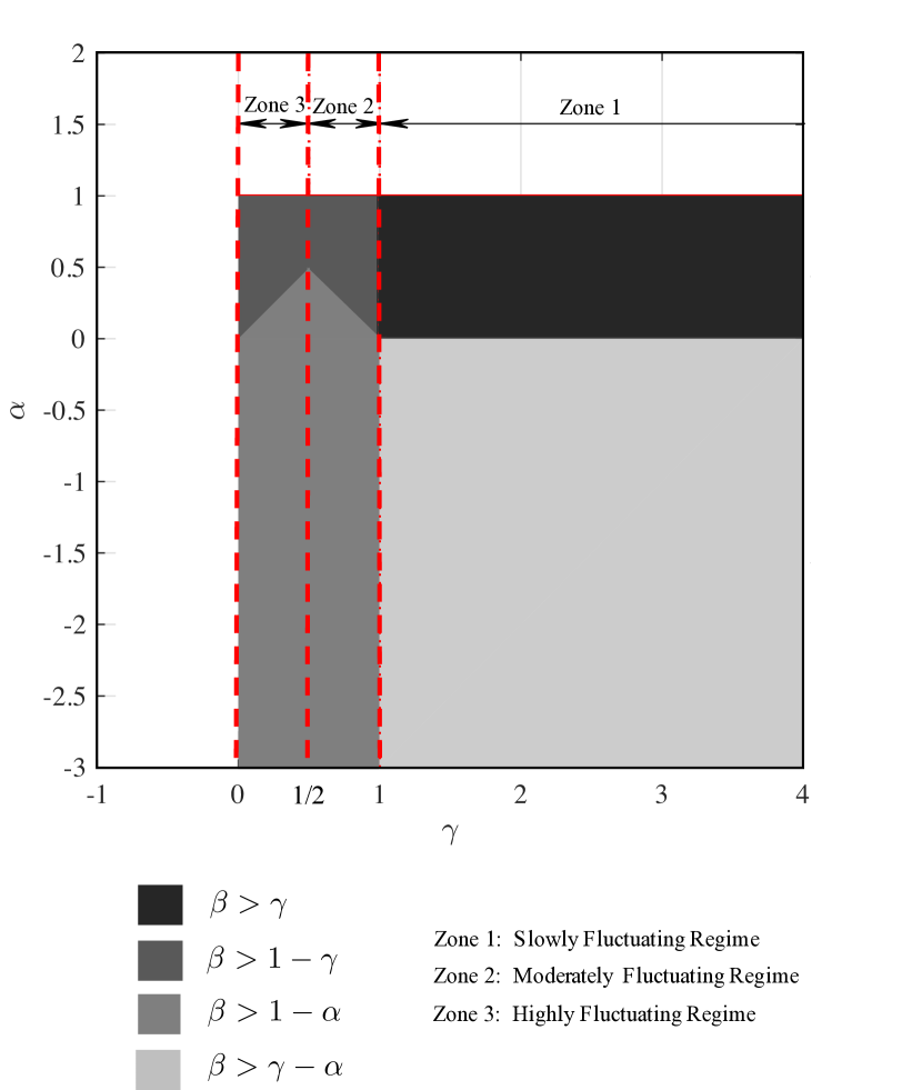
Figure 4: Diagram in the ($\alpha,\gamma$)-space summarizing the relationship between the Peclét $(=\omega^{\alpha})$, Damköhler $(=\omega^{\beta})$ and the ratio between space and time scale parameters $(\gamma=\mbox{log}\varepsilon/\mbox{log}\omega)$ in the three (slowly, moderately and highly fluctuating) regimes for a system with separation of scale parameter $\varepsilon\ll 1$ and boundary condition frequency $1/\omega\gg 1$.

The previous conditions are summarized in the $(\alpha,\gamma)$-plane of Figure 4.

The system behavior can be classified based on the magnitude of $\gamma$:

• When $\gamma>1$, i.e. $\varepsilon<\omega$, the system is referred to as slowly fluctuating; the conditions to guarantee that scale separation occur are summarized in the $(\alpha,\beta)$-plane in the Figure 1(a);

• When $1/2<\gamma<1$, i.e. $\omega<\varepsilon<\omega^{1/2}$ (or $\omega\approx\varepsilon$), the system is referred to as moderately fluctuating; the conditions to guarantee that scale separation occur are summarized in the $(\alpha,\beta)$-plane in the Figure 1(b);

• When $0<\gamma<1/2$, i.e. $\omega^{1/2}<\varepsilon<1$ (or $\varepsilon\gg\omega$), the system is referred to as highly fluctuating; the conditions to guarantee that scale separation occur are summarized in the $(\alpha,\beta)$-plane in the Figure 1(c).

A.3 Terms of Order $\mathcal{O}(\omega^{1})$

At the following order, we have Rearranging (LABEL:eq:a35) yields to

$$\left(\dfrac{\partial c_{1}}{\partial t}+\dfrac{\partial c_{2}}{\partial\tau}\right)-\nabla_{\mathbf{x}}\cdot(\textbf{D}\nabla_{\mathbf{x}}c_{1})-\omega^{-\gamma}[\nabla_{\mathbf{x}}\cdot(\textbf{D}\nabla_{\mathbf{y}}c_{1})]+$$

$$-\omega^{-\gamma}\nabla_{\mathbf{y}}\cdot\textbf{D}(\nabla_{\mathbf{x}}c_{1}+\omega^{1-\gamma}\nabla_{\mathbf{y}}c_{2})+\omega^{-\alpha}\nabla_{\mathbf{x}}\cdot(\mathbf{v}_{0}c_{1}+\mathbf{v}_{1}c_{0})+\omega^{1-\gamma-\alpha}\nabla_{\mathbf{y}}\cdot(\mathbf{v}_{0}c_{2}+\mathbf{v}_{1}c_{1}+\mathbf{v}_{2}c_{0})=0$$ (82)

subject to

$$-\mathbf{n}\cdot\mathbf{D}(\nabla_{\mathbf{x}}c_{1}+\omega^{1-\gamma}\nabla_{\mathbf{y}}c_{2})-\omega^{\beta}ac_{0}^{a-1}c_{1}=0.$$ (83)

Integrating (A.3) over $\mathcal{B}$ and $\mathcal{I}$ with respect to $\mathbf{y}$ and $\tau$, while accounting for (77), $\langle\chi\rangle=0$, we obtain,

$$\left\langle\dfrac{\partial c_{1}}{\partial t}\right\rangle_{\mathcal{IB}} +\left\langle\dfrac{\partial c_{2}}{\partial\tau}\right\rangle_{\mathcal{IB}}-\nabla_{\mathbf{x}}\cdot\left[\textbf{D}\nabla_{\mathbf{x}}\left(\left\langle\boldsymbol{\chi}(\mathbf{y},\tau)\right\rangle_{\mathcal{IB}}\cdot\nabla_{\mathbf{x}}c_{0}+\overline{c}_{1}(\mathbf{x},t)\right)\right]$$

$$-\omega^{-\gamma}\left[\nabla_{\mathbf{x}}\cdot\left\langle\textbf{D}\nabla_{\mathbf{y}}\left(\boldsymbol{\chi}(\mathbf{y},\tau)\cdot\nabla_{\mathbf{x}}c_{0}+\overline{c}_{1}(\mathbf{x},t)\right)\right\rangle_{\mathcal{IB}}\right]$$

$$-\omega^{-\gamma}\left\langle\nabla_{\mathbf{y}}\cdot\textbf{D}(\nabla_{\mathbf{x}}c_{1}+\omega^{1-\gamma}\nabla_{\mathbf{y}}c_{2})\right\rangle_{\mathcal{IB}}+\omega^{1-\gamma-\alpha}\left\langle\nabla_{\mathbf{y}}\cdot(\mathbf{v}_{0}c_{2}+\mathbf{v}_{1}c_{1}+\mathbf{v}_{2}c_{0})\right\rangle_{\mathcal{IB}}$$

$$+\omega^{-\alpha}\nabla_{\mathbf{x}}\cdot\left\langle\mathbf{v}_{0}c_{1}+\mathbf{v}_{1}c_{0}\right\rangle_{\mathcal{IB}}=0$$ (84)

The third term in (A.3) is identically equal to zero since $\langle\chi\rangle=0$ and the arbitrary integrating function $\overline{c}_{1}$ can be selected such that $\nabla_{\mathbf{x}}\cdot(\mathbf{D}\nabla_{\mathbf{x}}\overline{c}_{1})=0$, i.e. if $\overline{c}_{1}$ is linear in $\mathbf{x}$. Similarly, $\left\langle\nabla_{\mathbf{y}}\cdot(\mathbf{v}_{0}c_{2}+\mathbf{v}_{1}c_{1}+\mathbf{v}_{2}c_{0})\right\rangle_{\mathcal{IB}}=0$ because of the divergence theorem, the no-slip boundary condition on $\Gamma$ and periodicity on the unit cell boundaries. Therefore, (A.3) simplifies to

$$\left\langle\dfrac{\partial c_{1}}{\partial t}\right\rangle_{\mathcal{IB}} +\left\langle\dfrac{\partial c_{2}}{\partial\tau}\right\rangle_{\mathcal{IB}}-\omega^{-\gamma}\left[\nabla_{\mathbf{x}}\cdot\left(\left\langle\textbf{D}\nabla_{\mathbf{y}}\boldsymbol{\chi}(\mathbf{y},\tau)\right\rangle_{\mathcal{IB}}\cdot\nabla_{\mathbf{x}}c_{0}\right)\right]$$

$$+\omega^{-\alpha}\nabla_{\mathbf{x}}\cdot\left\langle\mathbf{v}_{0}c_{1}+\mathbf{v}_{1}c_{0}\right\rangle_{\mathcal{IB}}-\omega^{-\gamma}\left\langle\nabla_{\mathbf{y}}\cdot\textbf{D}(\nabla_{\mathbf{x}}c_{1}+\omega^{1-\gamma}\nabla_{\mathbf{y}}c_{2})\right\rangle_{\mathcal{IB}}=0.$$ (85)

We proceed further by analyzing the last two terms separately. We start with the fourth term in (A.3), $\nabla_{\mathbf{x}}\cdot\left\langle\mathbf{v}_{0}c_{1}+\mathbf{v}_{1}c_{0}\right\rangle_{\mathcal{IB}}$. Combining it with (77) and $\mathbf{v}_{0}=-\mathbf{k}(\mathbf{y})\cdot\nabla_{\mathbf{x}}P_{0}$ one obtains

$$\nabla_{\mathbf{x}}\cdot\left\langle\mathbf{v}_{0}c_{1}+\mathbf{v}_{1}c_{0}\right\rangle_{\mathcal{IB}}=-\nabla_{\mathbf{x}}\cdot\left\langle\mathbf{k}\nabla_{\mathbf{x}}P_{0}\left(\boldsymbol{\chi}\cdot\nabla_{\mathbf{x}}c_{0}+\overline{c}_{1}\right)\right\rangle_{\mathcal{IB}}+\nabla_{\mathbf{x}}\cdot\left\langle\mathbf{v}_{1}c_{0}\right\rangle_{\mathcal{IB}}.$$ (86)

Using Einstein notation convention and indicial notation, one can write

$$\nabla_{\mathbf{x}}\cdot\left\langle\mathbf{v}_{0}c_{1}+\mathbf{v}_{1}c_{0}\right\rangle_{\mathcal{IB}} =\frac{\partial}{\partial x_{i}}\left\langle v_{0i}c_{1}+v_{1i}c_{0}\right\rangle_{\mathcal{IB}}$$

$$=-\frac{\partial}{\partial x_{i}}\left\langle k_{ij}\frac{\partial P_{0}}{\partial x_{j}}\left(\chi_{m}\frac{\partial c_{0}}{\partial x_{m}}+\overline{c}_{1}\right)\right\rangle_{\mathcal{IB}}+\frac{\partial}{\partial x_{i}}\left\langle v_{1i}c_{0}\right\rangle_{\mathcal{IB}}$$

$$=-\left\langle k_{ij}\chi_{m}\right\rangle_{\mathcal{IB}}\left(\frac{\partial^{2}P_{0}}{\partial x_{i}\partial x_{j}}\frac{\partial c_{0}}{\partial x_{m}}+\frac{\partial P_{0}}{\partial x_{j}}\frac{\partial^{2}c_{0}}{\partial x_{i}\partial x_{m}}\right)$$

$$\quad\,-\left\langle k_{ij}\right\rangle_{\mathcal{IB}}\frac{\partial}{\partial x_{i}}\left(\frac{\partial P_{0}}{\partial x_{j}}\overline{c}_{1}\right)+\frac{\partial}{\partial x_{i}}\left\langle v_{1i}c_{0}\right\rangle_{\mathcal{IB}}.$$ (87)

Noticing that $\nabla_{\mathbf{x}}\cdot\langle\mathbf{v}_{0}\rangle_{\mathcal{IB}}\equiv 0$, this results in

$$\frac{\partial\langle v_{0i}\rangle_{\mathcal{IB}}}{\partial x_{i}}=-\frac{\partial}{\partial x_{i}}\left(\langle k_{ij}\rangle_{\mathcal{IB}}\frac{\partial P_{0}}{\partial x_{j}}\right)=-\langle k_{ij}\rangle_{\mathcal{IB}}\frac{\partial^{2}P_{0}}{\partial x_{i}\partial x_{j}}\equiv 0$$ (88)

i.e. $\partial_{x_{i}x_{j}}^{2}P_{0}\equiv 0$, since $\langle k_{ij}\rangle_{\mathcal{IB}}\neq 0$. Therefore, (A.3) can be simplified as follows

$$\nabla_{\mathbf{x}}\cdot\left\langle\mathbf{v}_{0}c_{1}+\mathbf{v}_{1}c_{0}\right\rangle_{\mathcal{IB}} =-\frac{\partial^{2}c_{0}}{\partial x_{i}\partial x_{m}}\left\langle\chi_{m}k_{ij}\right\rangle_{\mathcal{IB}}\frac{\partial P_{0}}{\partial x_{j}}-\frac{\partial}{\partial x_{i}}\left(\left\langle k_{ij}\right\rangle_{\mathcal{IB}}\frac{\partial P_{0}}{\partial x_{j}}\overline{c}_{1}\right)+\frac{\partial}{\partial x_{i}}\left\langle v_{1i}c_{0}\right\rangle_{\mathcal{IB}}$$

$$=-\left[\left\langle\boldsymbol{\chi}\mathbf{k}\right\rangle_{\mathcal{IB}}\cdot\nabla_{\mathbf{x}}P_{0}\right]_{mi}\frac{\partial}{\partial x_{i}}\left(\frac{\partial c_{0}}{\partial x_{m}}\right)$$

$$\quad-\frac{\partial}{\partial x_{i}}\left(\left[\left\langle\mathbf{k}\right\rangle_{\mathcal{IB}}\cdot\nabla_{\mathbf{x}}P_{0}\right]_{i}\overline{c}_{1}\right)+\frac{\partial}{\partial x_{i}}\left\langle v_{1i}c_{0}\right\rangle_{\mathcal{IB}}$$

$$=-\left[\left(\left\langle\boldsymbol{\chi}\mathbf{k}\right\rangle_{\mathcal{IB}}\cdot\nabla_{\mathbf{x}}P_{0}\right)\cdot\nabla_{\mathbf{x}}\right]\cdot\nabla_{\mathbf{x}}c_{0}$$

$$\quad-\nabla_{\mathbf{x}}\cdot\left(\left\langle\mathbf{k}\right\rangle_{\mathcal{IB}}\cdot\nabla_{\mathbf{x}}P_{0}\overline{c}_{1}\right)+\nabla_{\mathbf{x}}\cdot\left(\left\langle\mathbf{v}_{1}\right\rangle_{\mathcal{IB}}c_{0}\right)$$ (89)

Using the divergence theorem and the boundary condition (83), the last term in (A.3) can be written as

$$\omega^{-\gamma}\left\langle\nabla_{\mathbf{y}}\cdot\textbf{D}(\nabla_{\mathbf{x}}c_{1}+\omega^{1-\gamma}\nabla_{\mathbf{y}}c_{2})\right\rangle_{\mathcal{IB}}=-\omega^{\beta-\gamma}\mathcal{K^{\star}}ac_{0}^{a-1}\langle c_{1}\rangle_{\mathcal{I}\Gamma},$$ (90)

where $\mathcal{K^{\star}}=\dfrac{|\Gamma|}{|\mathcal{B}|}$. Inserting (A.3) and (90) in (A.3), white noting that $\langle A\rangle=\phi\langle A\rangle_{\mathcal{IB}}$ and $\overline{c}_{1}=\langle c_{1}\rangle$, we obtain

$$\left\langle\dfrac{\partial c_{1}}{\partial t}\right\rangle_{\mathcal{IB}} +\left\langle\dfrac{\partial c_{2}}{\partial\tau}\right\rangle_{\mathcal{IB}}-\phi^{-1}\omega^{-\gamma}\left[\nabla_{\mathbf{x}}\cdot\left(\left\langle\textbf{D}\nabla_{\mathbf{y}}\boldsymbol{\chi}\right\rangle\cdot\nabla_{\mathbf{x}}c_{0}\right)\right]-\phi^{-1}\omega^{-\alpha}\left[\left(\left\langle\boldsymbol{\chi}\mathbf{k}\right\rangle\cdot\nabla_{\mathbf{x}}P_{0}\right)\cdot\nabla_{\mathbf{x}}\right]\cdot\nabla_{\mathbf{x}}c_{0}$$

$$+\omega^{-\alpha}\nabla_{\mathbf{x}}\cdot\left(\left\langle\mathbf{v}_{0}\right\rangle_{\mathcal{IB}}\overline{c}_{1}\right)+\omega^{-\alpha}\nabla_{\mathbf{x}}\cdot\left(\left\langle\mathbf{v}_{1}\right\rangle_{\mathcal{IB}}c_{0}\right)+\omega^{\beta-\gamma}\mathcal{K^{\star}}ac_{0}^{a-1}\langle c_{1}\rangle_{\mathcal{I}\Gamma}=0.$$ (91)

Importantly, since $\left[\left(\left\langle\boldsymbol{\chi}\mathbf{k}\right\rangle\cdot\nabla_{\mathbf{x}}P_{0}\right)\cdot\nabla_{\mathbf{x}}\right]\cdot\nabla_{\mathbf{x}}c_{0}=\nabla_{\mathbf{x}}\cdot\left[\left(\left\langle\boldsymbol{\chi}\mathbf{k}\right\rangle\cdot\nabla_{\mathbf{x}}P_{0}\right)\cdot\nabla_{\mathbf{x}}c_{0}\right]$ because of (88), (A.3) can be rearranged as follows

$$\left\langle\dfrac{\partial c_{1}}{\partial t}\right\rangle_{\mathcal{IB}} +\left\langle\dfrac{\partial c_{2}}{\partial\tau}\right\rangle_{\mathcal{IB}}-\phi^{-1}\omega^{-1}\nabla_{\mathbf{x}}\cdot\left[\left(\omega^{1-\gamma}\left\langle\textbf{D}\nabla_{\mathbf{y}}\boldsymbol{\chi}\right\rangle+\omega^{1-\alpha}\left\langle\boldsymbol{\chi}\mathbf{k}\right\rangle\cdot\nabla_{\mathbf{x}}P_{0}\right)\cdot\nabla_{\mathbf{x}}c_{0}\right]$$

$$+\omega^{-\alpha}\nabla_{\mathbf{x}}\cdot\left(\left\langle\mathbf{v}_{0}\right\rangle_{\mathcal{IB}}\overline{c}_{1}+\left\langle\mathbf{v}_{1}\right\rangle_{\mathcal{IB}}c_{0}\right)+\omega^{\beta-\gamma}\mathcal{K^{\star}}ac_{0}^{a-1}\langle c_{1}\rangle_{\mathcal{I}\Gamma}=0.$$ (92)

Let

$$\tilde{\textbf{D}}^{\star}=\omega^{1-\gamma}\left\langle\textbf{D}\nabla_{\mathbf{y}}\boldsymbol{\chi}\right\rangle+\omega^{1-\alpha}\left\langle\boldsymbol{\chi}\mathbf{k}\right\rangle\cdot\nabla_{\mathbf{x}}P_{0}$$ (93)

$\tilde{\textbf{D}}^{\star}$ is a positive definite tensor. and $\textbf{D}^{\prime}$ is a positive dispersion vector. Accordingly, (A.3) can be written as

$$\omega\left\langle\dfrac{\partial c_{1}}{\partial t}\right\rangle_{\mathcal{IB}} +\omega\left\langle\dfrac{\partial c_{2}}{\partial\tau}\right\rangle_{\mathcal{IB}}-\phi^{-1}\nabla_{\mathbf{x}}\cdot\left(\tilde{\textbf{D}}^{\star}\cdot\nabla_{\mathbf{x}}\left\langle c_{0}\right\rangle\right)$$

$$+\omega^{1-\alpha}\nabla_{\mathbf{x}}\cdot\left(\left\langle\mathbf{v}_{0}\right\rangle_{\mathcal{IB}}\overline{c}_{1}+\left\langle\mathbf{v}_{1}\right\rangle_{\mathcal{IB}}c_{0}\right)+\omega^{\beta-\gamma}\mathcal{K^{\star}}\left(a\omega c_{0}^{a-1}\langle c_{1}\rangle_{\mathcal{I}\Gamma}\right)=0.$$ (94)

Calculating $\langle\partial c_{\omega}/\partial t\rangle_{\mathcal{IB}}$, while retaining terms up to the second order gives

$$\left\langle\dfrac{\partial c}{\partial t}\right\rangle_{\mathcal{IB}}=\dfrac{\partial c_{0}}{\partial t}+\left\langle\dfrac{\partial c_{1}}{\partial\tau}\right\rangle_{\mathcal{IB}}+\omega\left(\left\langle\dfrac{\partial c_{1}}{\partial t}\right\rangle_{\mathcal{IB}}+\left\langle\dfrac{\partial c_{2}}{\partial\tau}\right\rangle_{\mathcal{IB}}\right)+\mathcal{O}(\omega^{2}).$$ (95)

where $\left\langle\dfrac{\partial c}{\partial t}\right\rangle_{\mathcal{IB}}=\dfrac{\partial\left\langle c\right\rangle_{\mathcal{IB}}}{\partial t}$ because of the Leibniz rule. Adding (A.3) with (59) while accounting for (95), yields

$$\phi\dfrac{\partial\left\langle c\right\rangle_{\mathcal{IB}}}{\partial t} =\nabla_{\mathbf{x}}\cdot(\tilde{\textbf{D}}^{\star}\nabla_{\mathbf{x}}\left\langle c_{0}\right\rangle_{\mathcal{IB}})+\nabla_{\mathbf{x}}\cdot(\textbf{D}\nabla_{\mathbf{x}}\left\langle c_{0}\right\rangle_{\mathcal{IB}})$$

$$-\omega^{-\alpha}\nabla_{\mathbf{x}}\cdot\left(\omega\left\langle\mathbf{v}_{0}\right\rangle\overline{c}_{1}+\omega\left\langle\mathbf{v}_{1}\right\rangle c_{0}+c_{0}\langle\mathbf{v}_{0}\rangle_{\mathcal{IB}}\right)$$

$$+\phi\mathcal{K}^{\star}\omega^{\beta-\gamma}(1-c_{0}^{a}-a\omega c_{0}^{a-1}\langle c_{1}\rangle_{\mathcal{I}\Gamma}).$$ (96)

Since $\overline{c}_{1}=\langle c_{1}\rangle_{\mathcal{IB}}$ and $\langle c_{0}\rangle_{\mathcal{IB}}\langle\mathbf{v}_{0}\rangle=\langle c_{0}\rangle\langle\mathbf{v}_{0}\rangle_{\mathcal{IB}}$, then

$$\langle c\rangle_{\mathcal{IB}}\langle\mathbf{v}\rangle=\langle c_{0}\rangle\langle\mathbf{v}_{0}\rangle_{\mathcal{IB}}+\omega c_{0}\langle\mathbf{v}_{1}\rangle+\omega\overline{c}_{1}\langle\mathbf{v}_{0}\rangle+\mathcal{O}(\omega^{2}).$$ (97)

Assuming that $\quad\langle\chi\rangle_{\mathcal{I}\Gamma}\approx\langle\chi\rangle_{\mathcal{IB}}$, then $\langle c_{1}\rangle_{\mathcal{I}\Gamma}\approx\langle c_{1}\rangle_{\mathcal{IB}}$ and

$$\langle c_{0}\rangle_{\mathcal{IB}}^{a}+\omega a\langle c_{0}\rangle^{a-1}_{\mathcal{IB}}\langle c_{1}\rangle_{\mathcal{I}\Gamma}\approx\langle c_{0}\rangle_{\mathcal{IB}}^{a}+\omega a\langle c_{0}\rangle^{a-1}_{\mathcal{IB}}\langle c_{1}\rangle_{\mathcal{IB}}=\langle c\rangle^{a}_{\mathcal{IB}}+O(\omega^{2}).$$ (98)

Defining

$$\tilde{\tilde{\textbf{D}}}^{\star}=\langle\textbf{D}(\mathbf{I}+\omega^{1-\gamma}\nabla_{\mathbf{y}}\boldsymbol{\chi})\rangle+\omega^{1-\alpha}\langle\boldsymbol{\chi}\mathbf{k}\rangle\cdot\nabla_{\mathbf{x}}P_{0},$$ (99)

(A.3) becomes

$$\phi\dfrac{\partial\langle c\rangle_{\mathcal{IB}}}{\partial t}=\nabla\cdot(\tilde{\tilde{\textbf{D}}}^{\star}\nabla\langle c\rangle_{\mathcal{IB}}-\mbox{Pe}\langle c\rangle_{\mathcal{IB}}\langle\mathbf{v}\rangle)+\phi\omega^{-\gamma}\mathcal{K}^{\star}\mbox{Da}(1-\langle c\rangle_{\mathcal{IB}}^{a}),$$ (100)

which approximates the space-time average of $c_{\omega}$ up to an error of order $\omega^{2}$.

Appendix B Equations summary

B.1 Slowly Fluctuating Regimes: $\varepsilon<\omega$

B.1.1 $\mbox{Pe}<1$

$$\phi\dfrac{\partial\langle c\rangle_{\mathcal{IB}}}{\partial t}=\nabla\cdot\left[\tilde{\tilde{\textbf{D}}}^{\star}\nabla\langle c\rangle_{\mathcal{IB}}\right]+\phi\omega^{-\gamma}\mathcal{K}^{\star}\mbox{Da}(1-\langle c\rangle_{\mathcal{IB}}^{a}),$$

with

$$\tilde{\tilde{\textbf{D}}}^{\star}=\langle\textbf{D}(\mathbf{I}+\omega^{1-\gamma}\nabla_{\mathbf{y}}\boldsymbol{\chi})\rangle$$ (101)

and $\lambda$ and $\boldsymbol{\chi}$ defined as the solution of the following boundary value problem in the unit cell $\mathcal{B}$

$$\nabla_{\mathbf{y}}\cdot\textbf{D}(\mathbf{I}+\omega^{1-\gamma}\nabla_{\mathbf{y}}\boldsymbol{\chi})=0,\quad\mbox{subject to}\quad\mathbf{n}\cdot\textbf{D}(\mathbf{I}+\omega^{1-\gamma}\nabla_{\mathbf{y}}\boldsymbol{\chi})=0.$$ (102)

B.1.2 $1<\mbox{Pe}<\omega^{-1}$

$$\phi\dfrac{\partial\langle c\rangle_{\mathcal{IB}}}{\partial t}=\nabla\cdot\left[\tilde{\tilde{\textbf{D}}}^{\star}\nabla\langle c\rangle_{\mathcal{IB}}-\mbox{Pe}\langle c\rangle_{\mathcal{IB}}\langle\mathbf{v}\rangle_{\mathcal{IB}}\right]+\phi\omega^{-\gamma}\mathcal{K}^{\star}\mbox{Da}(1-\langle c\rangle_{\mathcal{IB}}^{a}),$$

with

$$\tilde{\tilde{\textbf{D}}}^{\star}=\langle\textbf{D}(\mathbf{I}+\omega^{1-\gamma}\nabla_{\mathbf{y}}\boldsymbol{\chi})\rangle+\omega^{1-\alpha}\langle\boldsymbol{\chi}\mathbf{k}\rangle\cdot\nabla_{\mathbf{x}}P_{0},$$ (103)

and $\boldsymbol{\chi}$ defined as the solution of the following boundary value problem in the unit cell $\mathcal{B}$

$$\textbf{ D}\nabla^{2}_{\mathbf{y}}\lambda=0,\quad\mbox{subject to}\quad\mathbf{n}\cdot\textbf{D}\nabla_{\mathbf{y}}\lambda=0\mbox{ on }\Gamma,$$

$$\nabla_{\mathbf{y}}\cdot\textbf{D}(\mathbf{I}+\omega^{1-\gamma}\nabla_{\mathbf{y}}\boldsymbol{\chi})=0,\quad\mbox{subject to}\quad\mathbf{n}\cdot\textbf{D}(\mathbf{I}+\omega^{1-\gamma}\nabla_{\mathbf{y}}\boldsymbol{\chi})=0\mbox{ on }\Gamma.$$ (104)

B.2 Moderately Fluctuating Regimes: $\omega^{1/2}<\varepsilon<1$

$$\phi\dfrac{\partial\langle c\rangle_{\mathcal{IB}}}{\partial t}=\nabla\cdot\left[\tilde{\tilde{\textbf{D}}}^{\star}\nabla\langle c\rangle_{\mathcal{IB}}-\mbox{Pe}\langle c\rangle_{\mathcal{IB}}\langle\mathbf{v}\rangle_{\mathcal{IB}}\right]+\phi\omega^{-\gamma}\mathcal{K}^{\star}\mbox{Da}(1-\langle c\rangle_{\mathcal{IB}}^{a}),$$

with

$$\tilde{\tilde{\textbf{D}}}^{\star}=\langle\textbf{D}(\mathbf{I}+\omega^{1-\gamma}\nabla_{\mathbf{y}}\boldsymbol{\chi})\rangle+\omega^{1-\alpha}\langle\boldsymbol{\chi}\mathbf{k}\rangle\cdot\nabla_{\mathbf{x}}P_{0}$$ (105)

and $\boldsymbol{\chi}$ defined as the solution of the following boundary value problem in the unit cell $\mathcal{B}$

$$\omega^{-\alpha}(\mathbf{v}_{0}-\langle\mathbf{v}_{0}\rangle)-\omega^{-\gamma}\nabla_{\mathbf{y}}\cdot\textbf{D}(\mathbf{I}+\omega^{1-\gamma}\nabla_{\mathbf{y}}\boldsymbol{\chi})+\omega^{1-\gamma-\alpha}\mathbf{v}_{0}\cdot(\nabla_{\mathbf{y}}\boldsymbol{\chi})=0,$$

$$\quad\mbox{subject to}\quad\mathbf{n}\cdot\textbf{D}(\mathbf{I}+\omega^{1-\gamma}\nabla_{\mathbf{y}}\boldsymbol{\chi})=0,\mbox{ on }\Gamma.$$ (106)

B.3 Higly Fluctuating Regimes: $\varepsilon\gg\omega$

B.3.1 $\mbox{Pe}<1$

$$\phi\dfrac{\partial\langle c\rangle_{\mathcal{IB}}}{\partial t}=\nabla\cdot\left[\tilde{\tilde{\textbf{D}}}^{\star}\nabla\langle c\rangle_{\mathcal{IB}}\right]+\phi\omega^{-\gamma}\mathcal{K}^{\star}\mbox{Da}(1-\langle c\rangle_{\mathcal{IB}}^{a}),$$

with

$$\tilde{\tilde{\textbf{D}}}^{\star}=\langle\textbf{D}(\mathbf{I}+\omega^{1-\gamma}\nabla_{\mathbf{y}}\boldsymbol{\chi})\rangle$$ (107)

and $\boldsymbol{\chi}$ defined as the solution of the following boundary value problem in the unit cell $\mathcal{B}$

$$\dfrac{\partial\boldsymbol{\chi}}{\partial\tau}-\omega^{-\gamma}\nabla_{\mathbf{y}}\cdot\textbf{D}(\mathbf{I}+\omega^{1-\gamma}\nabla_{\mathbf{y}}\boldsymbol{\chi})+\omega^{-\alpha}(\mathbf{v}_{0}-\langle\mathbf{v}_{0}\rangle)=0$$ (108)

subject to

$$-\mathbf{n}\cdot\textbf{D}(\mathbf{I}+\omega^{1-\gamma}\nabla_{\mathbf{y}}\boldsymbol{\chi})=0\quad\mbox{on}\quad\mathcal{\varGamma},$$

$$\boldsymbol{\chi}(\mathbf{y},\tau=0)=\boldsymbol{\chi}_{\tiny\mbox{in}}(\mathbf{y})=0.$$ (109)

B.3.2 $1<\mbox{Pe}<\omega^{-1}$

$$\phi\dfrac{\partial\langle c\rangle_{\mathcal{IB}}}{\partial t}=\nabla\cdot\left[\tilde{\tilde{\textbf{D}}}^{\star}\nabla\langle c\rangle_{\mathcal{IB}}-\mbox{Pe}\langle c\rangle_{\mathcal{IB}}\langle\mathbf{v}\rangle_{\mathcal{IB}}\right]+\phi\omega^{-\gamma}\mathcal{K}^{\star}\mbox{Da}(1-\langle c\rangle_{\mathcal{IB}}^{a}),$$

with

$$\tilde{\tilde{\textbf{D}}}^{\star}=\langle\textbf{D}(\mathbf{I}+\omega^{1-\gamma}\nabla_{\mathbf{y}}\boldsymbol{\chi})\rangle+\omega^{1-\alpha}\langle\boldsymbol{\chi}\mathbf{k}\rangle\cdot\nabla_{\mathbf{x}}P_{0}$$ (110)

and $\boldsymbol{\chi}$ defined as the solution of the following boundary value problem in the unit cell $\mathcal{B}$

$$\dfrac{\partial\chi}{\partial\tau}+\omega^{-\alpha}(\mathbf{v}_{0}-\langle\mathbf{v}_{0}\rangle)+\omega^{1-\gamma-\alpha}\mathbf{v}_{0}\cdot(\nabla_{\mathbf{y}}\boldsymbol{\chi})=0,$$

subject to

$$-\mathbf{n}\cdot\textbf{D}(\mathbf{I}+\omega^{1-\gamma}\nabla_{\mathbf{y}}\boldsymbol{\chi})=0\quad\mbox{on}\quad\mathcal{\varGamma},$$

$$\boldsymbol{\chi}(\mathbf{y},\tau=0)=\boldsymbol{\chi}_{\tiny\mbox{in}}(\mathbf{y})=0.$$ (111)

Appendix C Nomenclature

$$\mathcal{B}:\mbox{Pore-scale domain in the unit cell}\quad Y$$

$$\mathcal{I}:\mbox{Temporal unit cell}$$

$$c_{\omega}:\mbox{Dimensionless pore-scale concentration}$$

$$c_{\mbox{\tiny{in}}}(\mathbf{x}):\mbox{Dimensionless initial pore-scale concentration}$$

$$c_{D}(t):\mbox{Dimensionless time-varying concentration at a Dirichlet boundary $\partial\Omega_{D}$}$$

$$\langle c\rangle_{\mathcal{IB}}:\mbox{Average of pore-scale concentration over the pore volume $\mathcal{B}$ and the time interval $\mathcal{I}$}$$

$$\langle c\rangle:\mbox{Average of pore-scale concentration over the unit cell $Y$ and the time interval $\mathcal{I}$, such that $\langle c\rangle=\phi\langle c\rangle_{\mathcal{IB}}$}$$

$$\mathbf{D}:\mbox{Dimensionless molecular diffusion coefficient}$$

$$\mbox{Da}:\mbox{Damk\"{o}hler number}$$

$$\mbox{Pe}:\mbox{Pecl\'{e}t number}$$

$$l:\mbox{Characteristic length of periodic unit cell $Y$}$$

$$L:\mbox{Characteristic length of the macroscopic porous medium domain $\Omega$}$$

$$a:\mbox{Order of the heterogeneous reaction}$$

$$\hat{p}:\mbox{Dimensional dynamic pressure}$$

$$\mu:\mbox{Dynamic viscosity of the fluid}$$

$$\varepsilon=\dfrac{l}{L}:\mbox{Spatial scale separation parameter}$$

$$\omega=\dfrac{\hat{\tau}}{T}:\mbox{Temporal scale separation parameter}$$

$$\phi:\mbox{Unit cell porosity}$$

$$\hat{\Omega}:\mbox{Porous medium domain}$$

$$\hat{\Omega}_{p}:\mbox{Volume of the pore phase in $\hat{\Omega}$}$$

$$\hat{\Omega}_{s}:\mbox{Volume of the solid phase in $\hat{\Omega}$}$$

$$\partial\hat{\Omega}:\mbox{Outer boundary of the porous medium $\hat{\Omega}$}$$

$$\hat{\Gamma}:\mbox{Boundary between solid and pore phase}$$

$$\hat{\mathbf{v}}_{\varepsilon}:\mbox{Dimensional pore-scale velocity}$$

$$\boldsymbol{\chi}:\mbox{Closure variable in the unit cell}$$

$$\hat{Y}:\mbox{Unit cell domain}$$

$$\hat{\mathcal{B}}:\mbox{Solid phase in the unit cell domain $Y$}$$

$$\hat{\mathcal{G}}:\mbox{Pore phase in the unit cell domain $Y$}$$

$$\mathbf{x}:\mbox{Slow spatial scale}$$

$$t:\mbox{Slow time scale}$$

$$\mathbf{y}:\mbox{Fast spatial scale}$$

$$\tau:\mbox{Fast time scale}$$

$$U:\mbox{Characteristic velocity}$$

$$p:\mbox{Dimensionless pressure}$$

$$\hat{t}_{\mbox{\tiny{d,micro}}}:\mbox{Dimensional time-scale for diffusion at microscale}$$

$$\hat{t}_{\mbox{\tiny{d,macro}}}:\mbox{Dimensional time-scale for diffusion at microscale}$$

$$\hat{t}_{\mbox{\tiny{a,micro}}}:\mbox{Dimensional time-scale for advection at microscale}$$

$$\hat{t}_{\mbox{\tiny{a,macro}}}:\mbox{Dimensional time-scale for advection at macroscale}$$

$$\tau_{c}=\dfrac{L^{2}}{D}:\mbox{Characteristic time}$$

$$T:\mbox{Observation time-scale}$$

$$\hat{\tau}_{a}:\mbox{Advection time-scale}$$

$$\hat{\tau}_{d}:\mbox{Diffusion time-scale}$$

$$\hat{\tau}_{r}:\mbox{Reaction time-scale}$$

$$\hat{k}:\mbox{Dimensional pore-scale heterogeneous reaction rate}$$

$$\gamma:\mbox{The parameter connecting spatial and temporal scale separation parameters}$$

$$\psi_{\varepsilon}:\mbox{Any arbitrary pore-scale quantity}$$

$$\alpha:\mbox{Parameter defining Pecl\'{e}t, $\mbox{Pe}=\omega^{-\alpha}$}$$

$$\beta:\mbox{Parameter defining Damk\"{o}hler, $\mbox{Da}=\omega^{\beta}$}$$

$$\mathbf{K}:\mbox{Dimensionless permeability tensor}$$

$$\mathbf{k}:\mbox{Closure variable}$$

$$\mathbf{a}:\mbox{Closure variable}$$

$$\mathcal{K^{\star}}:\mbox{Effective reaction rate}$$

$$\tilde{\tilde{\textbf{D}}}^{\star}:\mbox{Effective dispersion tensor}$$

$$\nabla_{x}P_{0}:\mbox{Macroscopic pressure gradient}$$

$$\mathbf{n}:\mbox{Unit vector normal to the boundary}$$

$$c_{0},c_{1},c_{2},...:\mbox{Expansions of pore-scale concentration}$$

$$\mathbf{v}_{0},\mathbf{v}_{1},\mathbf{v}_{2},\cdots:\mbox{Expansions of pore-scale velocity}$$