Abstract

The dynamics of the gauge sector of QCD give rise to nonperturbative phenomena that are crucial for the internal consistency of the theory; most notably, they account for the generation of a gluon mass through the action of the Schwinger mechanism, the taming of the Landau pole and the ensuing stabilization of the gauge coupling, and the infrared suppression of the three-gluon vertex. In the present work, we review some key advances in the ongoing investigation of this sector within the framework of the continuum Schwinger function methods, supplemented by results obtained from lattice simulations.

1 1 0 https://doi.org/ Gauge Sector Dynamics in QCD Gauge sector dynamics in QCD Mauricio Narciso Ferreira^1,† and Joannis Papavassiliou^1,† Mauricio N. Ferreira and Joannis Papavassiliou Ferreira, M. N.; Papavassiliou, J. Correspondence: ansonar@uv.es (M. N. Ferreira); Joannis.Papavassiliou@uv.es (J. Papavassiliou) These authors contributed equally to this work.

1 Introduction

The systematic exploration of the Green’s functions ($n$-point correlation functions) of Quantum Chromodynamics (QCD) Marciano and Pagels (1978) by means of continuous Schwinger function methods Qin and Roberts (2020); Roberts (2020); Cui et al. (2020); Chang and Roberts (2021); Cui et al. (2022); Lu et al. (2022); Ding et al. (2022); Roberts (2022), such as Schwinger-Dyson equations (SDEs) Roberts and Williams (1994); Alkofer and von Smekal (2001); Fischer (2006); Roberts (2008); Binosi and Papavassiliou (2009); Bashir et al. (2012); Binosi et al. (2015); Cloet and Roberts (2014); Aguilar et al. (2016); Binosi et al. (2016, 2017); Huber (2020) and functional renormalization group Pawlowski et al. (2004); Pawlowski (2007); Fischer et al. (2009); Carrington (2013); Carrington et al. (2015); Cyrol et al. (2018); Corell et al. (2018); Huber (2020); Dupuis et al. (2021); Blaizot et al. (2021), together with a plethora of gauge-fixed lattice simulations Mandula and Ogilvie (1987); Parrinello (1994); Alles et al. (1997); Parrinello et al. (1998); Boucaud et al. (1998); Alexandrou et al. (2002); Bowman et al. (2002); Skullerud et al. (2003); Bowman et al. (2004); Cucchieri et al. (2006); Ilgenfritz et al. (2007); Sternbeck (2006); Furui and Nakajima (2006); Bowman et al. (2007); Kamleh et al. (2007); Cucchieri and Mendes (2007, 2008); Bogolubsky et al. (2007); Cucchieri et al. (2008); Cucchieri and Mendes (2008, 2010, 2009); Boucaud et al. (2009); Cucchieri et al. (2009); Bogolubsky et al. (2009); Oliveira and Silva (2009); Cucchieri et al. (2010); Oliveira and Bicudo (2011); Blossier et al. (2010); Cucchieri et al. (2010); Maas (2013); Boucaud et al. (2012); Ayala et al. (2012); Oliveira and Silva (2012); Sternbeck and Müller-Preussker (2013); Bicudo et al. (2015); Duarte et al. (2016); Athenodorou et al. (2016); Duarte et al. (2016); Oliveira et al. (2016); Boucaud et al. (2017); Sternbeck et al. (2017); Boucaud et al. (2018); Cucchieri et al. (2018a, b); Oliveira et al. (2019); Dudal et al. (2018); Vujinovic and Mendes (2019); Cui et al. (2020); Zafeiropoulos et al. (2019); Aguilar et al. (2020); Maas and Vujinović (2022); Kızılersü et al. (2021); Aguilar et al. (2021a, b); Pinto-Gómez et al. (2022); Pinto-Gomez and de Soto (2022); Pinto-Gómez et al. (2022), has afforded ample access to the dynamical mechanisms responsible for the nonperturbative properties of this remarkable theory. Particularly prominent in this quest is the notion of the emergent hadron mass (EHM) Roberts and Schmidt (2020); Roberts (2020, 2021); Roberts et al. (2021); Binosi (2022); Papavassiliou (2022); Ding et al. (2022); Roberts (2022), together with its three supporting pillars: first, the generation of a gluon mass Cornwall (1979); Parisi and Petronzio (1980); Cornwall (1982); Bernard (1982, 1983); Donoghue (1984); Mandula and Ogilvie (1987); Cornwall and Papavassiliou (1989); Lavelle (1991); Halzen et al. (1993); Wilson et al. (1994); Mihara and Natale (2000); Philipsen (2002); Kondo (2001); Aguilar et al. (2003); Aguilar and Natale (2004); Aguilar and Papavassiliou (2006); Epple et al. (2008); Aguilar and Papavassiliou (2007); Aguilar et al. (2008); Aguilar and Papavassiliou (2010); Campagnari and Reinhardt (2010); Fagundes et al. (2012); Aguilar et al. (2011, 2012a, 2012b, 2013, 2016); Glazek et al. (2017); Binosi and Papavassiliou (2018); Aguilar et al. (2019); Eichmann et al. (2021); Aguilar et al. (2022); Horak et al. (2022); Papavassiliou (2022); Aguilar et al. (2022) through the action of the Schwinger mechanism Schwinger (1962a, b); second, the construction of the process-independent effective charge Cornwall (1982); Watson (1997); Binosi and Papavassiliou (2003); Aguilar et al. (2009); Binosi et al. (2015, 2017); Cui et al. (2020); Roberts (2020), which arises as the QCD analogue of the Gell-Mann–Low charge known from Quantum Electrodynamics (QED) Gell-Mann and Low (1954); Itzykson and Zuber (1980), and has associated to it a renormalization-group invariant (RGI) scale of about half of the proton mass Binosi et al. (2017); Cui et al. (2020); and third, the dynamical breaking of chiral symmetry and the generation of constituent quark masses Nambu and Jona-Lasinio (1961); Lane (1974); Politzer (1976); Miransky and Fomin (1981); Atkinson and Johnson (1988); Brown and Pennington (1988); Williams et al. (1991); Papavassiliou and Cornwall (1991); Hawes et al. (1994); Roberts and Williams (1994); Natale and Rodrigues da Silva (1997); Fischer and Alkofer (2003); Maris and Roberts (2003); Aguilar et al. (2005); Bowman et al. (2005); Sauli et al. (2007); Cornwall (2008); Alkofer et al. (2009); Aguilar and Papavassiliou (2011); Cloet and Roberts (2014); Rojas et al. (2013); Mitter et al. (2015); Braun et al. (2016); Heupel et al. (2014); Binosi et al. (2017); Aguilar et al. (2018); Gao et al. (2021).

The dynamics of the gauge sector of QCD, which encompasses both gluonic and ghost interactions, is instrumental for the physical picture of the EHM outlined above. In fact, the basic concepts and pivotal mechanisms sustaining the first two pillars of the EHM have their original inception and most genuine realization in the realm of pure Yang-Mills theories Eichten and Feinberg (1974); Smit (1974); Cornwall (1979, 1982); Aguilar and Papavassiliou (2006); Aguilar et al. (2008); Binosi et al. (2012); Aguilar et al. (2016, 2012a); Papavassiliou (2022). Therefore, in the present review, we focus precisely on the rich dynamical content of the gauge sector, especially in relation with the generation of a gluon mass scale out of the intricate gluon self-interactions.

The formulation of the nonperturbative QCD physics in terms of the Green’s functions of the fundamental degrees of freedom, such as gluon and ghost propagators and vertices, provides an intuitive framework for unraveling a wide array of subtle mechanisms; in fact, certain distinctive features of these functions have been inextricably connected with key phenomena such as gluon mass generation, violation of reflection positivity, and confinement, to name a few. Thus, the saturation of the gluon propagator in the deep infrared Alexandrou et al. (2002); Cucchieri and Mendes (2007, 2008); Bogolubsky et al. (2007, 2009); Oliveira and Silva (2009); Oliveira and Bicudo (2011); Cucchieri and Mendes (2010); Cucchieri et al. (2009, 2010); Sternbeck and Müller-Preussker (2013); Bicudo et al. (2015); Bowman et al. (2007); Kamleh et al. (2007); Ayala et al. (2012); Duarte et al. (2016); Dudal et al. (2018); Aguilar et al. (2020) has been interpreted as the unequivocal signal of a gluon mass Smit (1974); Cornwall (1982); Bernard (1982, 1983); Donoghue (1984); Mandula and Ogilvie (1987); Cornwall and Papavassiliou (1989); Wilson et al. (1994); Philipsen (2002); Aguilar et al. (2003); Aguilar and Natale (2004); Aguilar and Papavassiliou (2006); Aguilar et al. (2008); Tissier and Wschebor (2010); Binosi et al. (2012); Serreau and Tissier (2012); Peláez et al. (2014); Siringo (2016); Aguilar et al. (2016); and the existence of an inflection point in the same function has been argued to lead to a non-positive gluon spectral density Ding et al. (2022), and the ensuing loss of reflection positivity Osterwalder and Schrader (1973, 1975); Glimm and Jaffe (1981); Krein et al. (1992); Alkofer and von Smekal (2001); Roberts (2008); Cornwall (2013); Binosi et al. (2015); Ding et al. (2022) for the dressed gluons. Similarly, the masslessness of the ghost induces Aguilar et al. (2014) a maximum in the gluon propagator, and a zero crossing in the form factors of the three-gluon vertex Cucchieri et al. (2008); Aguilar et al. (2014); Pelaez et al. (2013); Blum et al. (2014); Eichmann et al. (2014); Williams et al. (2016); Blum et al. (2015); Cyrol et al. (2016); Athenodorou et al. (2016); Duarte et al. (2016); Boucaud et al. (2017); Sternbeck et al. (2017); Corell et al. (2018); Aguilar et al. (2019, 2020, 2021a); Barrios et al. (2022), followed by an infrared divergence for vanishing momenta. The dynamical origin of these special traits will be the focal point of the analysis presented in the main body of this article.

The integral equations that govern the full momentum evolution of the Green’s functions, known as SDEs, constitute the indispensable formal and practical instrument for unraveling the special characteristics mentioned above. In their primordial form, the SDEs are rigorously derived from the generating functional of the theory Rivers (1988); Itzykson and Zuber (1980), and encode all dynamical information on the correlation functions, within the entire range of physical momenta. In practice, due to the enormous complexity of these equations, approximations and truncations need to be implemented; but, unlike perturbation theory, no expansion parameter is available in the strongly coupled regime of the theory for carrying out such a task. Despite this intrinsic shortcoming, in recent years the SDE predictions have become particularly robust, in part due to various theoretical advances, and in part thanks to the intense synergy with gauge-fixed lattice simulations, as will be evidenced in the subsequent sections.

Typically, the Green’s function of QCD are defined within the quantization scheme obtained by implementing the linear covariant ($R_{\xi}$) gauges Fujikawa et al. (1972). The corresponding SDEs are derived and solved within this same quantization scheme, and in particular in the Landau gauge ($\xi=0$), where lattice simulations are almost exclusively performed; for studies away from the Landau gauge, see e.g., Epple et al. (2008); Aguilar and Papavassiliou (2008); Cucchieri et al. (2009); Campagnari and Reinhardt (2010); Huber et al. (2010); Cucchieri et al. (2010); Siringo (2014); Bicudo et al. (2015); Aguilar et al. (2015); Huber (2015); Capri et al. (2015); Aguilar et al. (2017); Glazek et al. (2017); Cucchieri et al. (2018a, b); De Meerleer et al. (2020); Napetschnig et al. (2021). A great deal may be learned, however, by considering the Green’s functions and corresponding SDEs formulated within the “PT-BFM”scheme Aguilar and Papavassiliou (2006); Binosi and Papavassiliou (2008), namely the framework that arises from the fusion of the pinch technique (PT) Cornwall (1982); Cornwall and Papavassiliou (1989); Pilaftsis (1997); Binosi and Papavassiliou (2002, 2004, 2009) with the background field method (BFM) DeWitt (1967); ’t Hooft (1971); Honerkamp (1972); Kallosh (1974); Kluberg-Stern and Zuber (1975); Arefeva et al. (1974); Abbott (1981); Weinberg (1980); Abbott (1982); Shore (1981); Abbott et al. (1983). The main advantage of the PT-BFM originates from the fact that certain appropriately chosen Green’s functions satisfy Abelian Slavnov-Taylor identities (STIs), whose tree-level form does not get modified by quantum corrections. This situation is to be contrasted to the standard STIs Taylor (1971); Slavnov (1972) obtained in the conventional framework of the linear covariant gauges, which are deformed by non-trivial contributions stemming from the gauge sector of the theory. In the present work, we will carry out computations and develop arguments within both frameworks ($R_{\xi}$ and PT-BFM), and will elaborate on their connection by means of the so-called Background-Quantum identities (BQIs) Grassi et al. (2001a, b); Binosi and Papavassiliou (2002, 2009).

The article is organized as follows:

$\bullet$ In Section 2 we introduce some basic notation and review certain prominent features of the Green’s functions within both the linear gauges and the PT-BFM formalism Aguilar and Papavassiliou (2006); Binosi and Papavassiliou (2008). We stress, in particular, the properties of the auxiliary function $G(q)$ Aguilar et al. (2009, 2009); Binosi and Quadri (2013); Binosi et al. (2015), which relates the gluon propagators with quantum and background gluons, and is intimately connected with the definition of the process-independent and RGI interaction strength Binosi et al. (2015), to be discussed in detail in Section 6. In addition, we elucidate with a concrete example the important property of “block-wise” transversality, displayed by the background gluon self-energy Aguilar and Papavassiliou (2006); Aguilar et al. (2008, 2016).

$\bullet$ In Section 3 we review the general principles associated with the Schwinger mechanism Schwinger (1962a, b) that endows gauge bosons with an effective mass, focusing on the details associated with its realization in the context of Yang-Mills theories. We place particular emphasis on the pivotal requirement that must be satisfied by the fundamental vertices of the theory, namely the appearance of massless poles in their form factors Eichten and Feinberg (1974); Aguilar and Papavassiliou (2006, 2007); Aguilar et al. (2008); Aguilar and Papavassiliou (2010); Aguilar et al. (2012a); Ibañez and Papavassiliou (2013); Aguilar et al. (2016); Papavassiliou (2022).

$\bullet$ In Section 4 we examine the dynamical formation of colored composite excitations (bound states) of vanishing mass, which provide the required structures in the vertices, in order for the Schwinger mechanism to be activated Eichten and Feinberg (1974); Aguilar et al. (2012a); Ibañez and Papavassiliou (2013); Aguilar et al. (2016). The formation of these states out of a pair of gluons or a ghost–antighost pair is controlled by a set of coupled Bethe-Salpeter equations (BSEs) Aguilar et al. (2012a); Ibañez and Papavassiliou (2013); Aguilar et al. (2016, 2018, 2022), which are found to have nontrivial solutions for the corresponding Bethe-Salpeter (BS) amplitudes, to be denoted by ${\mathbb{C}}(r)$ and ${\mathcal{C}}(r)$, respectively.

$\bullet$ In Section 5 we explain in detail how the presence of the massless poles in the dressed vertices that enter in the SDE of the gluon propagator gives rise to a gluon mass. The demonstration is carried out separately for the $g_{\mu\nu}$ and $q_{\mu}q_{\nu}/q^{2}$ components of the gluon self-energy. The former case requires the evasion of the so-called “seagull identity” Aguilar and Papavassiliou (2010); Aguilar et al. (2016); this becomes possible by virtue of the crucial Ward identity (WI) displacement, to be further considered in Section 10.

$\bullet$ In Section 6 we go over the basic notions underpinning the PT Cornwall (1982); Cornwall and Papavassiliou (1989); Pilaftsis (1997); Binosi and Papavassiliou (2002, 2009), and show how their application leads naturally to the definition of a dimensionful process-independent RGI interaction strength Cornwall (1982); Watson (1997); Binosi and Papavassiliou (2003); Aguilar et al. (2009); Binosi et al. (2015, 2017); Cui et al. (2020); Roberts (2020), denoted by ${\widehat{d}}(q)$. The genuine process-independence of this quantity is concretely exemplified by demonstrating its appearance in two processes involving fundamentally different external fields. Next, ${\widehat{d}}(q)$ is computed by combining lattice data for the gluon propagator and SDE results for the function $G(q)$. Finally, the dimensionless quantity is derived that constitutes the physical definition of the one-gluon exchange interaction appearing in standard bound-state computations Munczek (1995); Bender et al. (1996); Maris et al. (1998); Maris and Roberts (1997); Chang and Roberts (2009); Chang et al. (2011); Bashir et al. (2012); Cloet and Roberts (2014); Binosi et al. (2015); Qin and Roberts (2021).

$\bullet$ In Section 7 we focus on the structure of the “transversely projected” three-gluon vertex Eichmann et al. (2014); Blum et al. (2014); Huber (2016); Aguilar et al. (2022), and discuss briefly the property of planar degeneracy Pinto-Gómez et al. (2022), satisfied, at a high level of accuracy Eichmann et al. (2014); Blum et al. (2014); Huber (2016); Pinto-Gómez et al. (2022); Pinto-Gomez and de Soto (2022); Pinto-Gómez et al. (2022), by the vertex form factors. This special property induces a striking simplification to the structure of this vertex, captured by a particularly compact expression Pinto-Gómez et al. (2022), which will be extensively used in some of the following sections.

$\bullet$ In Section 8 we take a close look at the ghost sector of the theory, and solve the coupled system of SDEs governing the ghost propagator and ghost-gluon vertex Schleifenbaum et al. (2005); Boucaud et al. (2008); Huber and von Smekal (2013); Aguilar et al. (2013, 2019, 2021b); as is well-known, the ghost remains massless, but its dressing function saturates at the origin Ilgenfritz et al. (2007); Cucchieri and Mendes (2007); Bogolubsky et al. (2007); Cucchieri and Mendes (2008); Aguilar et al. (2008); Dudal et al. (2008); Boucaud et al. (2008, 2008); Bogolubsky et al. (2009); Kondo (2010); Boucaud et al. (2012); Pennington and Wilson (2011); Dudal et al. (2012); Ayala et al. (2012); Aguilar et al. (2013); Cyrol et al. (2016); Huber (2020); Boucaud et al. (2018); Aguilar et al. (2019); Cui et al. (2020); Aguilar et al. (2021b), because the infrared-finite gluon propagator used in the ghost SDE provides an effective infrared cutoff. In the SDE of the ghost-gluon vertex, we employ as central input the compact expression for the three-gluon vertex presented in the previous section. The results are in excellent agreement with the available lattice data for the ghost dressing function Boucaud et al. (2018); Aguilar et al. (2021b) and the form factor of the ghost-gluon vertex evaluated in the soft-gluon limit Ilgenfritz et al. (2007); Sternbeck (2006).

$\bullet$ In Section 9 we discuss two important consequences of the masslessness of the ghost propagator, which manifest themselves at the level of both the gluon propagator and the three-gluon vertex. Specifically, the diagrams comprised by a ghost loop induce “unprotected” logarithms, i.e., of the type $\ln q^{2}$; instead, gluonic loops give rise to “protected” logarithms, of the type $\ln(q^{2}+m^{2})$, where $m$ is the effective gluon mass Aguilar et al. (2014); Papavassiliou et al. (2022). As $q^{2}\to 0$, the unprotected contributions diverge, driving the appearance of a maximum in the gluon propagator and a divergence in its first derivative, as well as a zero-crossing and a corresponding divergence in the form factors of the three-gluon vertex. As we comment in this section, of particular phenomenological importance Meyers and Swanson (2013); Sanchis-Alepuz et al. (2015); Xu et al. (2019); Souza et al. (2020); Huber et al. (2020, 2021); Papavassiliou et al. (2022) is the relative suppression that the above features induce to the dominant vertex form factors in the intermediate range of momenta.

$\bullet$ In Section 10 we discuss an outstanding feature of the WI satisfied by the pole-free part of the three-gluon vertex, namely the displacement induced by the presence of the aforementioned massless poles Aguilar et al. (2022); Papavassiliou (2022). In this context, we introduce the key quantity denominated “displacement function”, whose appearance serves as a smoking gun signal of the action of the Schwinger mechanism in QCD; quite interestingly, it coincides Aguilar et al. (2022); Papavassiliou (2022) with the BS amplitude ${\mathbb{C}}(r)$ for the formation of a massless scalar out of a pair of gluons, introduced in Section 4. In addition, we derive a crucial relation, which ultimately permits the indirect determination of ${\mathbb{C}}(r)$ from lattice QCD Aguilar et al. (2022); Papavassiliou (2022); Aguilar et al. (2022); an important ingredient in this relation is a partial derivative Aguilar et al. (2020, 2022), denoted by ${\cal W}(r)$, of the ghost-gluon kernel Aguilar et al. (2019), to be determined in the next section.

$\bullet$ In Section 11 we set up and solve the SDE that governs the evolution of ${\cal W}(r)$ Aguilar et al. (2020, 2021, 2022, 2022); the main component of this SDE is a special projection of the three-gluon vertex, which is computed by appealing to formulas established in Section 7, and allows for the accurate determination of ${\cal W}(r)$ in the entire range of relevant momenta Aguilar et al. (2022).

$\bullet$ In Section 12 we substitute into the central relation derived in Section 10 the solution for ${\cal W}(r)$ found in the previous section, together with the lattice data Aguilar et al. (2021b, a) for the gluon propagator, the ghost dressing function, and the form factor of the three-gluon vertex associated with the soft-gluon limit, in order to obtain the form of the displacement function ${\mathbb{C}}(r)$ Aguilar et al. (2022, 2022). As we discuss, the results exclude with nearly absolute certainty the null hypothesis (absence of Schwinger mechanism, ${\mathbb{C}}(r)=0$), and corroborate the action of the Schwinger mechanism in QCD Aguilar et al. (2022). In addition, we show that the form of ${\mathbb{C}}(r)$ found is statistically completely compatible with that obtained from the BSE-based analysis presented in Section 4.

$\bullet$ In Section 13 we present our conclusions.

$\bullet$ Finally, in Appendix A we derive the BQIs relating the displacement functions of the conventional and background vertices.

2 Basic concepts and general theoretical framework

We start by considering the Lagrangian density of an SU($N$) Yang-Mills theory, comprised of the classical part, ${\cal L}_{\mathrm{cl}}$, the contribution from the ghosts, ${\cal L}_{\mathrm{gh}}$, and the covariant gauge-fixing term, ${\cal L}_{\mathrm{gf}}$, namely

$${\cal L}_{\mathrm{YM}}={\cal L}_{\mathrm{cl}}+{\cal L}_{\mathrm{gh}}+{\cal L}_{\mathrm{gf}}\,,$$ (1)

where

$${\cal L}_{\mathrm{cl}}=-\frac{1}{4}F^{a}_{\mu\nu}F^{a\mu\nu}\,,\qquad{\cal L}_{\mathrm{gh}}=-{\overline{c}}^{a}\partial^{\mu}D_{\mu}^{ab}c^{b}\,,\qquad{\cal L}_{\mathrm{gf}}=\frac{1}{2\xi}(\partial^{\mu}A^{a}_{\mu})^{2}\,.$$ (2)

In the above formula, $A^{a}_{\mu}(x)$ denotes the gauge field, while $c^{a}(x)$ and ${\overline{c}}^{a}(x)$ represent the ghost and antighost fields, respectively, with $a=1,\dots,N^{2}-1$.

In addition,

$$F^{a}_{\mu\nu}=\partial_{\mu}A^{a}_{\nu}-\partial_{\nu}A^{a}_{\mu}+gf^{abc}A^{b}_{\mu}A^{c}_{\nu}\,,$$ (3)

is the antisymmetric field tensor, where $f^{abc}$ stands for the totally antisymmetric structure constants of the SU($N$) gauge group, and $g$ is the gauge coupling, while

$$D_{\mu}^{ab}=\partial_{\mu}\delta^{ac}+gf^{amb}A^{m}_{\mu}\,,$$ (4)

denotes the covariant derivative in the adjoint representation. Finally, $\xi$ represents the gauge-fixing parameter; the choice $\xi=0$ corresponds to the Landau gauge, while $\xi=1$ specifies the Feynman -´t Hooft gauge.

The transition from the pure Yang-Mills theory of Eq. (1) to QCD is implemented by supplementing the corresponding kinetic and interaction terms for the quark fields. However, since throughout this work we do not consider effects due to dynamical quarks, the aforementioned terms will be omitted entirely.

The most fundamental correlation function is the gluon propagator, whose nonperturbative features are inextricably connected with key dynamical properties of the theory. In the Landau gauge that we will employ throughout, the gluon propagator, $\Delta^{ab}_{\mu\nu}(q)=-i\delta^{ab}\Delta_{\mu\nu}(q)$, is completely transverse, i.e.,

$$\Delta_{\mu\nu}(q)=\Delta(q){P}_{\mu\nu}(q)\,,\qquad{P}_{\mu\nu}(q):=g_{\mu\nu}-q_{\mu}q_{\nu}/{q^{2}}\,.$$ (5)

In the continuum, the dynamical properties of the gluon propagator are encoded in the corresponding SDE, given by

$$\Delta^{-1}(q)P_{\mu\nu}(q)=q^{2}P_{\mu\nu}(q)+i{\Pi}_{\mu\nu}(q)\,,$$ (6)

where $\Pi_{\mu\nu}(q)$ is the gluon self-energy, shown diagrammatically in the first row of Fig. 1. The fully-dressed vertices entering the diagrams are determined by their own SDEs, obtaining finally a tower of coupled integral equations, which, for practical purposes, must be truncated or treated approximately.

Given that, by virtue of the fundamental STI satisfied by the two-point function, the self-energy $\Pi_{\mu\nu}(q)$ is transverse,

$$q^{\mu}\Pi_{\mu\nu}(q)=0\,,$$ (7)

we have that

$$\Pi_{\mu\nu}(q)=\Pi(q)P_{\mu\nu}(q)\,,$$ (8)

and from Eq. (6) follows that

$$\Delta^{-1}(q)=q^{2}+i\Pi(q)\,.$$ (9)

Of particular importance is the exact way that Eq. (7) is enforced at the level of the SDE given in Fig. 6, which governs the gluon evolution. In particular, note that, if we were to contract the corresponding diagrams by $q^{\mu}$, the entire set of diagrams must be considered in order for Eq. (7) to emerge from the SDE. This pattern manifests itself already at the one-loop level, where it is known that the ghost-loop must be included in order to guarantee the transversality of the self-energy. The main practical drawback stemming from this observation is that truncations, in the form of omission of certain subsets of graphs, are likely to distort this fundamental property.

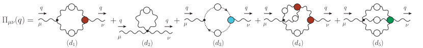
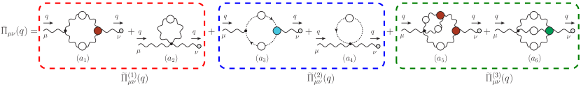
Figure 1: Upper panel: the diagrammatic representation of the conventional gluon self-energy, $\Pi_{\mu\nu}(q)$. Bottom panel: the diagrammatic representation of the $Q^{a}_{\mu}(q)B^{b}_{\nu}(-q)$, self-energy $\delta^{ab}{\widetilde{\Pi}}_{\mu\nu}(q)$; the grey circles at the end of the gluon lines indicate a background gluon. The corresponding Feynman rules are given in Appendix B of Binosi and Papavassiliou (2009).

Quite interestingly, within the PT-BFM framework the transversality property of Eq. (7) is enforced in a very special way, which permits physically meaningful truncations. In what follows we will employ predominantly the language of the BFM; for the basic principles of the PT and its connection with the BFM, the reader is referred to the extended literature on the subject Cornwall (1982); Cornwall and Papavassiliou (1989); Pilaftsis (1997); Binosi and Papavassiliou (2002, 2002, 2009); Cornwall et al. (2010), as well as to Section 6 of the present work.

The BFM is a powerful quantization procedure, where the gauge-fixing is implemented without compromising explicit gauge invariance. Within this framework the gauge field $A$ appearing in the classical action is decomposed as $A=B+Q$, where $B$ and $Q$ are the background and quantum (fluctuating) fields, respectively. Note that the variable of integration in the generating functional $Z(J)$ is the quantum field, which couples to the external sources, as $J\cdot Q$. The background field does not appear in loops. Instead, it couples externally to the Feynman diagrams, connecting them with the asymptotic states to form elements of the S-matrix. Then, if the gauge-fixing term

$${\widehat{\cal L}}_{\mathrm{gf}}=\frac{1}{2\xi_{{\scriptscriptstyle Q}}}({\widehat{D}}_{\mu}^{ab}Q^{b\mu})^{2}\,,\qquad{\widehat{D}}_{\mu}^{ab}=\partial_{\mu}\delta^{ab}+gf^{amb}B_{\mu}^{m}\,,$$ (10)

is used, the resulting gauge-fixed action retains its invariance under gauge transformations of the background field. As a result of this invariance, when the Green’s functions are contracted by the momentum carried by a background gluon, they satisfy Abelian (ghost-free) STIs, akin to the Takahashi identities known from QED. In particular, the STIs of the BFM retain their tree-level form to all orders, in contradistinction to the STIs of the $R_{\xi}$ gauges, whose form is modified by contributions stemming from the ghost sector.

Within the BFM, one may consider three kinds of propagators, by choosing the type of incoming and outgoing gluons Binosi and Papavassiliou (2008). In particular, we have:

(i) The propagator $\langle 0|\,T\![Q^{a}_{\mu}(q)Q^{b}_{\nu}(-q)]\!|0\rangle$ that connects two quantum gluons. Notice that this propagator coincides with the conventional gluon propagator of the covariant gauges, defined in Eq. (5), under the assumption that the corresponding gauge-fixing parameters, $\xi$ and $\xi_{{\scriptscriptstyle Q}}$, are identified, i.e., $\xi=\xi_{{\scriptscriptstyle Q}}$.

(ii) The propagator $\langle 0|\,T\![Q^{a}_{\mu}(q)B^{b}_{\nu}(-q)]\!|0\rangle$ that connects a $Q^{a}_{\mu}(q)$ with a $B^{b}_{\nu}(-q)$, to be denoted by $\widetilde{\Delta}^{ab}_{\mu\nu}(q)=-i\delta^{ab}\widetilde{\Delta}_{\mu\nu}(q)$.

(iii) The propagator $\langle 0|\,T\![B^{a}_{\mu}(q)B^{b}_{\nu}(-q)]\!|0\rangle$ that connects a $B^{a}_{\mu}(q)$ with a $B^{b}_{\nu}(-q)$, to be denoted by $\widehat{\Delta}^{ab}_{\mu\nu}(q)=-i\delta^{ab}\widehat{\Delta}_{\mu\nu}(q)$. Note that its full definition requires an additional gauge-fixing term, with the associated “classical” gauge-fixing parameter, $\xi_{{\scriptscriptstyle C}}$ Abbott (1981); Abbott et al. (1983); Binosi and Papavassiliou (2009).

Given that the relations captured by Eqs. (5) and (6) apply also in the cases of $\widetilde{\Delta}_{\mu\nu}(q)$ and $\widehat{\Delta}_{\mu\nu}(q)$, one may define the corresponding self-energies $\widetilde{\Pi}_{\mu\nu}(q)$ and $\widehat{\Pi}_{\mu\nu}(q)$, as well as the functions $\widetilde{\Delta}(q)$ and $\widehat{\Delta}(q)$.

Table 1: The different types of gluon propagators of the background field method (BFM), together with their diagrammatic representations, symbols, corresponding self-energies, and the background quantum identities (BQIs) that relate them to the conventional propagator.

External legs	Diagrammatic representation	Symbol	Self-energy	BQI
$Q^{a}_{\mu}(q)Q^{b}_{\nu}(-q)$		-iδ^abΔ_μν(q)	Π_μν(q)	—
$Q^{a}_{\mu}(q)B^{b}_{\nu}(-q)$		-iδ^ab~Δ_μν(q)	~Π_μν(q)	~Δ(q) = Δ(q)1 + G(q)
$B^{a}_{\mu}(q)B^{b}_{\nu}(-q)$		-iδ^ab^Δ_μν(q)	^Π_μν(q)	^Δ(q) = Δ(q)[1 + G(q)]2

Quite interestingly, the three propagators defined in (i)-(iii) are related by a set of exact identities, known as BQIs Grassi et al. (2001a, b); Binosi and Papavassiliou (2002, 2009). In particular, we have that (see also Table 1)

$$\Delta(q)=[1+G(q)]\widetilde{\Delta}(q)=[1+G(q)]^{2}\widehat{\Delta}(q)\,,$$ (11)

where the function $G(q)$ is the $g_{\mu\nu}$ component of a particular two-point ghost function, $\Lambda_{\mu\nu}(q)$, given by Grassi et al. (2001a); Binosi and Papavassiliou (2002); Grassi et al. (2004); Binosi and Quadri (2013)

$$\Lambda_{\mu\nu}(q):=ig^{2}C_{\rm A}\int_{k}\Delta^{\rho}_{\mu}(k)D(k+q)H_{\nu\rho}(-q,k+q,-k)=g_{\mu\nu}G(q)+\frac{q_{\mu}q_{\nu}}{q^{2}}L(q)\,,$$ (12)

where $C_{\mathrm{A}}$ is the Casimir eigenvalue of the adjoint representation [$N$ for SU$(N)$], $D^{ab}(q)=i\delta^{ab}D(q)$ is the ghost propagator, and $H_{\nu\mu}(r,p,q)$ denotes the ghost-gluon kernel defined in Fig. 2.

In the Landau gauge, a special identity relates the form factors of $\Lambda_{\mu\nu}(q)$ to the ghost dressing function, $F(q)$, defined as $F(q)=q^{2}D(q)$, namely Aguilar et al. (2009); Binosi and Quadri (2013); Binosi et al. (2015)

$$F^{-1}(q)=1+G(q)+L(q)\,,$$ (13)

which is valid before renormalization. In fact, in this particular gauge, $G(q)$ coincides with the so-called Kugo-Ojima function Kugo ; Grassi et al. (2004); Kondo (2009); Aguilar et al. (2009).

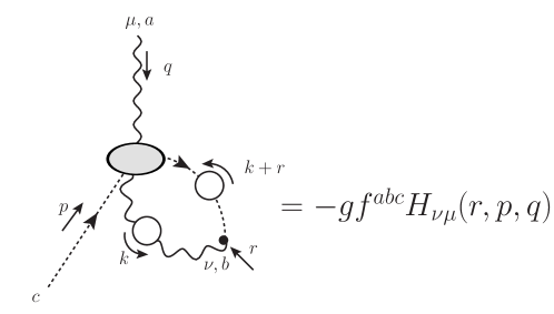
Figure 2: Diagrammatic definition of the ghost-gluon scattering kernel, $H_{\nu\mu}(r,p,q)$. At tree level, $H_{\nu\mu}^{0}=g_{\nu\mu}$.

To determine the renormalized form of Eq. (13), we introduce the renormalization constants of the conventional Green’s functions

$$\Delta_{{\rm{\scriptscriptstyle R}}}(q)=Z_{A}^{-1}\Delta(q)\,,\qquad F_{{\rm{\scriptscriptstyle R}}}(q)=Z_{c}^{-1}F(q)\,,$$ (14)

$${\rm{I}}\!\Gamma_{\mu}^{{\rm{\scriptscriptstyle R}}}(r,p,q)=Z_{1}{\rm{I}}\!\Gamma_{\mu}(r,p,q)\,,\qquad {\rm{I}}\!\Gamma_{\alpha\mu\nu}^{{\rm{\scriptscriptstyle R}}}(q,r,p)=Z_{3}{\rm{I}}\!\Gamma_{\alpha\mu\nu}(q,r,p)\,,$$

$$g_{{\rm{\scriptscriptstyle R}}}=Z_{g}^{-1}g\,,\qquad \left[g_{\mu\nu}+\Lambda_{\mu\nu}^{{\rm{\scriptscriptstyle R}}}(q)\right]=Z_{\Lambda}\left[g_{\mu\nu}+\Lambda_{\mu\nu}(q)\right]\,,$$

$$Z_{g}^{-1}=Z_{1}^{-1}Z_{A}^{1/2}Z_{c}=Z_{3}^{-1}Z_{A}^{3/2}\,,$$

where we denote by ${\rm{I}}\!\Gamma^{abc}_{\mu}(r,p,q)=-gf^{abc}{\rm{I}}\!\Gamma_{\mu}(r,p,q)$ and ${\rm{I}}\!\Gamma^{abc}_{\alpha\mu\nu}(q,r,p)=gf^{abc}{\rm{I}}\!\Gamma_{\alpha\mu\nu}(q,r,p)$ the conventional ghost-gluon [$Q^{a}_{\mu}(q)c^{c}(p){\bar{c}}^{b}(r)$] and three-gluon [$Q^{a}_{\alpha}(q)Q^{b}_{\mu}(r)Q^{c}_{\nu}(p)$] vertices, respectively. Note that, by virtue of Taylor’s theorem Taylor (1971), $Z_{1}$ is finite in the Landau gauge; its precise value depends on the renormalization scheme adopted, see Sec. 8. Moreover, denoting by ${\widehat{Z}}_{A}$ the (wave-function) renormalization constant of $\widehat{\Delta}(q)$, the Abelian STIs of the BFM impose the validity of the pivotal relation Abbott (1981); Abbott et al. (1983); Binosi and Papavassiliou (2009)

$$Z_{g}={\widehat{Z}}_{A}^{-1/2}\,,$$ (15)

which is the non-Abelian analogue of the textbook relation $Z_{e}=Z_{A}^{-1/2}$ Itzykson and Zuber (1980), relating the renormalization constants of the electric charge and the photon propagator in QED.

Then, since the BQIs of Eq. (11) are direct consequences of the Becchi-Rouet-Stora-Tyutin (BRST) symmetry Becchi et al. (1975, 1976); Tyutin (1975) of the theory Grassi et al. (2001a); Binosi and Papavassiliou (2002); Grassi et al. (2004); Binosi and Quadri (2013), their form is preserved by renormalization. Hence, combining Eqs. (11), (15) and (14) we obtain

$$Z_{\Lambda}=Z_{1}^{-1}Z_{c}\,,$$ (16)

which yields

$$Z^{-1}_{1}F^{-1}(q)=1+G(q)+L(q)\,.$$ (17)

As has been shown in Aguilar et al. (2009), the dynamical equation governing $L(q)$ yields $L(0)=0$, provided that the gluon propagator entering in it is finite at the origin. Thus, one obtains from Eq. (17) the useful identity Aguilar et al. (2009)

$$Z^{-1}_{1}F^{-1}(0)=1+G(0)\,.\,$$ (18)

According to numerous lattice simulations and studies in the continuum (see, e.g., Ilgenfritz et al. (2007); Cucchieri and Mendes (2007); Bogolubsky et al. (2007); Cucchieri and Mendes (2008); Aguilar et al. (2008); Dudal et al. (2008); Boucaud et al. (2008, 2008); Bogolubsky et al. (2009); Kondo (2010); Boucaud et al. (2012); Pennington and Wilson (2011); Dudal et al. (2012); Ayala et al. (2012); Aguilar et al. (2013); Cyrol et al. (2016); Huber (2020); Boucaud et al. (2018); Aguilar et al. (2019); Cui et al. (2020); Aguilar et al. (2021b)), the ghost dressing function reaches a finite (nonvanishing) value at the origin, which, due to Eq. (18), furnishes also the value of $G(0)$.

The final upshot of the above considerations is that one may use the BQIs in Eq. (11) to express the SDE given in Eq. (6) in terms of the $\widetilde{\Pi}_{\mu\nu}(q)$ or $\widehat{\Pi}_{\mu\nu}(q)$, at the modest cost of introducing in the dynamics the quantities $1+G(q)$ or $[1+G(q)]^{2}$. Focusing on the former possibility, Eq. (11) becomes

$$\Delta^{-1}(q)P_{\mu\nu}(q)=\frac{q^{2}P_{\mu\nu}(q)+i{\widetilde{\Pi}}_{\mu\nu}(q)}{1+G(q)}\,,$$ (19)

where the diagrammatic representation of the self-energy ${\widetilde{\Pi}}_{\mu\nu}(q)$ is shown in the lower panel of Fig. 1.

The principal advantage of this formulation is that the self-energy ${\widetilde{\Pi}}_{\mu\nu}(q)$ contains fully-dressed vertices with a background gluon of momentum $q$ exiting from them, which satisfy Abelian STIs. In particular, denoting by $\widetilde{{\rm{I}}\!\Gamma}_{\mu\alpha\beta}(q,r,p)$, $\widetilde{{\rm{I}}\!\Gamma}_{\mu}(r,p,q)$, and $\widetilde{{\rm{I}}\!\Gamma}^{mnrs}_{\mu\alpha\beta\gamma}(q,r,p,t)$ the BQQ, Bcc, and BQQQ vertices, respectively, we have that Cornwall and Papavassiliou (1989); Aguilar and Papavassiliou (2006); Binosi and Papavassiliou (2009)

$$q^{\mu}\widetilde{{\rm{I}}\!\Gamma}_{\mu\alpha\beta}(q,r,p) = \Delta_{\alpha\beta}^{-1}(r)-\Delta_{\alpha\beta}^{-1}(p)\,,$$ (20)

$$q^{\mu}\widetilde{{\rm{I}}\!\Gamma}_{\mu}(r,p,q) = {D}^{-1}(p)-{D}^{-1}(r)\,,$$ (21)

$$q^{\mu}\widetilde{{\rm{I}}\!\Gamma}^{mnrs}_{\mu\alpha\beta\gamma}(q,r,p,t) = f^{mse}f^{ern}{{\rm{I}}\!\Gamma}_{\alpha\beta\gamma}(r,p,q+t)+f^{mne}f^{esr}{{\rm{I}}\!\Gamma}_{\beta\gamma\alpha}(p,t,q+r)$$ (22)

$$+ f^{mre}f^{ens}{{\rm{I}}\!\Gamma}_{\gamma\alpha\beta}(t,r,q+p)\,.$$

In contrast, the conventional three-gluon and ghost-gluon vertices, ${\rm{I}}\!\Gamma_{\alpha\mu\nu}(q,r,p)$ and ${\rm{I}}\!\Gamma_{\alpha}(r,p,q)$, respectively, satisfy the STIs Marciano and Pagels (1978); Ball and Chiu (1980); Davydychev et al. (1996); von Smekal et al. (1998); Binosi and Papavassiliou (2011); Gracey et al. (2019)

$$q^{\alpha}{\rm{I}}\!\Gamma_{\alpha\mu\nu}(q,r,p)=F(q)\left[\Delta^{-1}(p)P_{\nu}^{\sigma}(p)H_{\sigma\mu}(p,q,r)-\Delta^{-1}(r)P_{\mu}^{\sigma}(r)H_{\sigma\nu}(r,q,p)\right]\,,$$ (23)

$$q^{\mu}F^{-1}(q){\rm{I}}\!\Gamma_{\mu}(r,p,q)+p^{\mu}F^{-1}(p){\rm{I}}\!\Gamma_{\mu}(r,q,p)=-r^{2}F^{-1}(r)U(r,q,p)\,,$$ (24)

where $U(r,q,p)$ is an interaction kernel containing only ghost fields; its tree level value is $U^{0}(r,q,p)=1$. The STI for the conventional four-gluon vertex is given in Eq. (C.24) of Binosi and Papavassiliou (2009).

The special STIs listed in Eqs. (20), (21) and (22) are responsible for the remarkable property of “block-wise” transversality Aguilar and Papavassiliou (2006); Binosi and Papavassiliou (2008, 2008), displayed by ${\widetilde{\Pi}}_{\mu\nu}(q)$. To appreciate this point, notice that the diagrams comprising ${\widetilde{\Pi}}_{\mu\nu}(q)$ in Fig. 1 have been separated into three different subsets (blocks) comprised of: (i) one-loop dressed diagrams containing only gluons, (ii) one-loop dressed diagrams containing a ghost loop, and (iii) two-loop dressed diagrams containing only gluons. The corresponding contributions of each block to ${\widetilde{\Pi}}_{\mu\nu}(q)$ are denoted by ${\widetilde{\Pi}}^{(i)}_{\mu\nu}(q)$, with $i=1,2,3$.

The block-wise transversality is a stronger version of the standard transversality relation $q^{\mu}{\widetilde{\Pi}}_{\mu\nu}(q)=0$; it states that each block of diagrams mentioned above is individually transverse, namely

$$q^{\mu}{\widetilde{\Pi}}^{(i)}_{\mu\nu}(q)=0\,,\qquad i=1,2,3.$$ (25)

In order to appreciate in detail the reason why the STIs in Eqs. (20), (21) and (22) are instrumental for the block-wise transversality, we will consider the case of ${\widetilde{\Pi}}^{(2)}_{\mu\nu}(q)$; the relevant diagrams are enclosed by the blue box of Fig. 1.

The diagrams $(a_{3})$ and $(a_{4})$ are given by

$$(a_{3})_{\mu\nu}(q) =g^{2}C_{\rm A}\int_{k}(k+q)_{\mu}D(k+q)D(k)\widetilde{{\rm{I}}\!\Gamma}\vphantom{{\rm{I}}\!\Gamma}_{\nu}(-k,k+q,-q)\,,$$ (26)

$$(a_{4})_{\mu\nu}(q) =g^{2}C_{\rm A}\,g_{\mu\nu}\int_{k}D(k)\,,$$ (27)

where a color factor $\delta^{ab}$ has been suppressed in both expressions. In addition, for the formal manipulations of integrals, we employ dimensional regularization Collins (1986); to that end, we introduce the short-hand notation

$$\int_{k}:=\frac{\mu_{{\scriptscriptstyle 0}}^{\epsilon}}{(2\pi)^{d}}\!\int_{-\infty}^{+\infty}\!\!\mathrm{d}^{d}k\,,$$ (28)

where $d=4-\epsilon$ is the dimension of the space-time, and $\mu_{{\scriptscriptstyle 0}}$ denotes the ’t Hooft mass.

The contraction of graph $(a_{3})_{\mu\nu}(q)$ by $q^{\nu}$ triggers the STI satisfied by $\widetilde{\Gamma}\vphantom{\Gamma}_{\nu}(-k,k+q,-q)$ [given by Eq. (21)], and we obtain

$$q^{\nu}(a_{3})_{\mu\nu}(q) = g^{2}C_{\rm A}\int_{k}(k+q)_{\mu}D(k+q)D(k)\left[D^{-1}(k)-D^{-1}(k+q)\right]$$ (29)

$$= g^{2}C_{\rm A}\int_{k}(k+q)_{\mu}\left[D(k+q)-D(k)\right]$$

$$= -g^{2}C_{\rm A}\,q_{\mu}\int_{k}D(k)\,,$$

which is precisely the negative of the contraction $q^{\nu}(a_{4})_{\mu\nu}(q)$. Hence,

$$q^{\nu}\left[(a_{3})_{\mu\nu}(q)+(a_{4})_{\mu\nu}(q)\right]=0\,.$$ (30)

3 Schwinger mechanism in Yang-Mills theories

The BRST symmetry of the Yang-Mills Lagrangian given in Eq. (1) prohibits the inclusion of a mass term of the form $m^{2}A^{2}_{\mu}$. Moreover, a symmetry-preserving regularization scheme, such as dimensional regularization, prevents the generation of a mass term at any finite order in perturbation theory. Nonetheless, as affirmed four decades ago Cornwall (1979); Parisi and Petronzio (1980); Cornwall (1982); Bernard (1982, 1983); Donoghue (1984), the nonperturbative Yang-Mills dynamics endow the gluons with an effective mass, which sets the scale for all dimensionful quantities, and tames the instabilities originating from the infrared divergences of the perturbative expansion (e.g., Landau pole). In addition, the presence of this mass causes the effective decoupling (screening) of the gluonic modes beyond a “maximum gluon wavelength” Brodsky and Shrock (2008), and leads to the dynamical suppression of the Gribov copies, see, e.g., Braun et al. (2010); Binosi et al. (2015); Gao et al. (2018) and references therein.

The generation of a gluon mass proceeds through the nonperturbative realization of the Schwinger mechanism Schwinger (1962a, b). Even though the technical details associated with the implementation of this mechanism in a four-dimensional non-Abelian setting are particularly elaborate, the general underlying idea is relatively easy to convey.

To that end, consider the dimensionless vacuum polarization ${\bf\Pi}(q)$, defined through ${\Pi}(q)=q^{2}{\bf\Pi}(q)$, such that

$$\Delta^{-1}({q})=q^{2}[1+i{\bf\Pi}(q)]\,.$$ (31)

The Schwinger mechanism is based on the fundamental observation that, if ${\bf\Pi}(q)$ develops a pole at $q^{2}=0$ (to be referred to as “massless pole”) then the vector meson (gluon) picks up a mass, regardless of any “prohibition” imposed by the gauge symmetry at the level of the original Lagrangian. Thus, in Euclidean space, the above sequence of ideas leads to

$$\lim_{q\to 0}{\bf\Pi}(q)=m^{2}/q^{2}\,\,\Longrightarrow\,\,\lim_{q\to 0}\,\Delta^{-1}(q)=\lim_{q\to 0}\,(q^{2}+m^{2})\,\,\Longrightarrow\,\,\Delta^{-1}(0)=m^{2}\,,$$ (32)

and the gauge boson propagator saturates to a non-zero value at the origin. This effect of infrared saturation of the propagator signifies the generation of a mass, which is identified with the positive residue of the pole.

At this descriptive level, Schwinger’s argument is completely general, making no particular reference to the specific dynamics that would lead to the appearance of the required massless pole inside ${\bf\Pi}(q)$. In fact, depending on the particular theory, the field-theoretic circumstances that trigger the crucial sequence captured by Eq. (32) may be very distinct, see, e.g.,  Jackiw and Johnson (1973); Jackiw (1973). In the case of Yang-Mills theories, the origin of the massless poles is purely nonperturbative Eichten and Feinberg (1974): the strong dynamics produce scalar composite excitations, which carry color and have vanishing masses. These poles are carried by the fully-dressed vertices of the theory; and since these vertices enter in the gluon SDE shown in Fig. 1 [upper (lower) panel for the QQ (QB) propagator], the massless poles find their way into the gluon self-energy (or, equivalently, the gluon vacuum polarization). The detailed implementation of this idea has been presented in a series of works Eichten and Feinberg (1974); Smit (1974); Cornwall (1982); Papavassiliou (1990); Aguilar et al. (2008, 2012a, 2012b); Binosi et al. (2012); Aguilar et al. (2012a, 2011, 2016, 2016, 2017); Papavassiliou (2022), and will be summarized in the rest of this section.

Let us focus for now on the conventional three-gluon and ghost-gluon vertices, ${\rm{I}}\!\Gamma_{\alpha\mu\nu}(q,r,p)$ and ${\rm{I}}\!\Gamma_{\alpha}(r,p,q)$, respectively, introduced below Eq. (14). When the formation of massless poles is triggered, these vertices assume the general form (see Fig. 3)

$${\rm{I}}\!\Gamma_{\alpha\mu\nu}(q,r,p) = \Gamma_{\alpha\mu\nu}(q,r,p)+V_{\alpha\mu\nu}(q,r,p)\,,\qquad$$

$${\rm{I}}\!\Gamma_{\alpha}(r,p,q) = \Gamma_{\alpha}(r,p,q)+V_{\alpha}(r,p,q)\,,$$ (33)

where $\Gamma_{\alpha\mu\nu}(q,r,p)$ and $\Gamma_{\alpha}(r,p,q)$ are their pole-free components, while $V_{\alpha\mu\nu}(q,r,p)$ and $V_{\alpha}(q,r,p)$ contain longitudinally coupled poles, whose special tensorial structure is given by

$$V_{\alpha\mu\nu}(q,r,p) = \frac{q_{\alpha}}{q^{2}}C_{\mu\nu}(q,r,p)+\frac{r_{\mu}}{r^{2}}A_{\alpha\nu}(q,r,p)+\frac{p_{\nu}}{p^{2}}B_{\alpha\mu}(q,r,p)\,,$$

$$V_{\alpha}(r,p,q) = \frac{q_{\alpha}}{q^{2}}C(r,p,q)\,,$$ (34)

such that

$${P}_{\alpha^{\prime}}^{\alpha}(q){P}_{\mu^{\prime}}^{\mu}(r){P}_{\nu^{\prime}}^{\nu}(p)V_{\alpha\mu\nu}(q,r,p)=0\,,\qquad{P}_{\alpha^{\prime}}^{\alpha}(q)V_{\alpha}(r,p,q)=0\,.$$ (35)

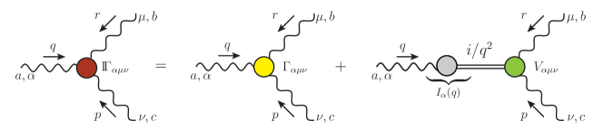
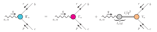
Figure 3: The diagrammatic representation of the three-gluon and ghost-gluon vertices introduced in Eq. (33): ${\rm{I}}\!\Gamma_{\alpha\mu\nu}(q,r,p)$ (first row) and ${\rm{I}}\!\Gamma_{\alpha}(r,p,q)$ (second row). The first term on the r.h.s. indicates the pole-free part, $\Gamma_{\alpha\mu\nu}(q,r,p)$ or $\Gamma_{\alpha}(r,p,q)$, while the second denotes the pole term $V_{\alpha\mu\nu}(q,r,p)$ or $V_{\alpha}(r,p,q)$.

We emphasize that the reason why $V_{\alpha\mu\nu}(q,r,p)$ and $V_{\alpha}(q,r,p)$ are longitudinally coupled may be directly inferred from their special decomposition, shown in Fig. 3. In particular, let us denote by $I_{\alpha}(q)$ the transition amplitude that connects a gluon with a massless composite scalar, depicted as a gray circle in Fig. 3. Since $I_{\alpha}(q)$ depends solely on the momentum $q$, and carries a single Lorentz index, $\alpha$, its general form is given by $I_{\alpha}(q)=q_{\alpha}I(q)$, where $I(q)$ is a scalar form factor Aguilar et al. (2012a); Ibañez and Papavassiliou (2013). This observation accounts directly for the form of $V_{\alpha}(q,r,p)$ given in Eq. (34); to deduce the form of $V_{\alpha\mu\nu}(q,r,p)$, one must, in addition, appeal to Bose symmetry, which imposes the structures $r_{\mu}/r^{2}$ and $p_{\nu}/p^{2}$ in the remaining two channels.

Returning to the SDE of Eq. (1), the component $V_{\alpha\mu\nu}(q,r,p)$ will enter in it through graphs ($d_{1}$) and $(d_{4})$, while the component $V_{\alpha}(q,r,p)$ through graph ($d_{3}$). Since $V_{\alpha\mu\nu}(q,r,p)$ has poles for each one of its three momenta, let us point out that only the pole associated with the $q$-channel, i.e., the channel that carries the momentum entering in the gluon propagator, is relevant for the Schwinger mechanism that will generate mass for $\Delta(q)$. In fact, in the Landau gauge that we employ, the gluon propagators inside the diagrams ($d_{1}$) and $(d_{4})$ are transverse, leading to a considerable reduction in the number of the form factors of $V_{\alpha\mu\nu}(q,r,p)$ that participate actively, since

$${P}_{\mu^{\prime}}^{\mu}(r){P}_{\nu^{\prime}}^{\nu}(p)V_{\alpha\mu\nu}(q,r,p)=\frac{q_{\alpha}}{q^{2}}{P}_{\mu^{\prime}}^{\mu}(r){P}_{\nu^{\prime}}^{\nu}(p)C_{\mu\nu}(q,r,p)\,.$$ (36)

Consequently, for the ensuing analysis, one requires only the tensorial decomposition of the component $C_{\mu\nu}(q,r,p)$ in Eq. (34), which is given by

$$C_{\mu\nu}(q,r,p)=C_{1}\,g_{\mu\nu}+C_{2}\,r_{\mu}r_{\nu}+C_{3}\,p_{\mu}p_{\nu}+C_{4}\,r_{\mu}p_{\nu}+C_{5}\,p_{\mu}r_{\nu}\,,$$ (37)

where $C_{j}:=C_{j}(q,r,p)$. Then, the substitution of Eq. (37) into Eq. (36), and use of the relation $q+p+r=0$, reveals that only two form factors survive inside ($d_{1}$) and $(d_{4})$, namely

$${P}_{\mu^{\prime}}^{\mu}(r){P}_{\nu^{\prime}}^{\nu}(p)V_{\alpha\mu\nu}(q,r,p)=\frac{q_{\alpha}}{q^{2}}{P}_{\mu^{\prime}}^{\mu}(r){P}_{\nu^{\prime}}^{\nu}(p)\left[C_{1}\,g_{\mu\nu}+C_{5}q_{\mu}q_{\nu}\right]\,.$$ (38)

Since the main function of the Schwinger mechanism is to make the gluon propagator saturate at the origin, it is important to explore the properties of the structures appearing in Eq. (38) near $q=0$. To that end, we expand the r.h.s. of Eq. (38), keeping terms at most linear in $q$. After noticing that the term proportional to $C_{5}$ in Eq. (38) is of order ${\cal O}(q^{2})$, we end up with a single relevant form factor associated with $V_{\alpha\mu\nu}(q,r,p)$, namely $C_{1}(q,r,p)$, which survives the $q\to 0$ limit of graphs ($d_{1}$) and $(d_{4})$. As for $V_{\alpha}(r,p,q)$, its unique component, $C(q,r,p)$, enters directly in ($d_{3}$).

The continuation of this analysis entails the Taylor expansion of $C_{1}(q,r,p)$ and $C(r,p,q)$ around $q=0$. In carrying out this expansion, one employs the following two key relations,

$$C_{1}(0,r,-r)=0\,,\qquad\qquad C(r,-r,0)=0\,.$$ (39)

The first one follows directly from the Bose symmetry of the three-gluon vertex, which implies that $C_{1}(q,r,p)=-C_{1}(q,p,r)$; as we will see in Sec. 10, it may also be derived in a completely independent way from the fundamental STIs satisfied by the three-gluon vertex. The justification of the second relation in Eq. (39) is less straightforward; its derivation, presented in Appendix A, relies on the BQI Binosi and Papavassiliou (2002, 2009) linking the conventional ghost-gluon vertex, ${\rm{I}}\!\Gamma_{\alpha}(r,p,q)$, with its background counterpart, $\widetilde{{\rm{I}}\!\Gamma}\vphantom{{\rm{I}}\!\Gamma}_{\alpha}(r,p,q)$.

Thus, after taking Eq. (39) into account, the Taylor expansion of ${C}_{1}(q,r,p)$ and ${C}(r,p,q)$ around $q=0$ yields

$$\lim_{q\to 0}{C}_{1}(q,r,p)=2(q\cdot r){\mathbb{C}}(r)\,+\cdots\,,\qquad\lim_{q\to 0}{C}(r,p,q)=2(q\cdot r){\mathcal{C}}(r)\,+\cdots\,,$$ (40)

with

$${\mathbb{C}}(r):=\left[\frac{\partial{C}_{1}(q,r,p)}{\partial p^{2}}\right]_{q=0}\,,\qquad\qquad{\mathcal{C}}(r):=\left[\frac{\partial{C}(r,p,q)}{\partial p^{2}}\right]_{q=0}\,.$$ (41)

The functions ${\mathbb{C}}(r)$ and ${\mathcal{C}}(r)$ are of central importance for the rest of this review. In particular, there are three key points related to them that will be elucidated in detail in what follows:

1. ${\mathbb{C}}(r)$ and ${\mathcal{C}}(r)$ are the BS amplitudes describing the formation of gluon-gluon and ghost-antighost colored composite bound states, respectively, see Sec. 4.

2. The gluon mass is determined by certain integrals that involve ${\mathbb{C}}(r)$ and ${\mathcal{C}}(r)$, given explicitly in Sec. 5.

3. ${\mathbb{C}}(r)$ and ${\mathcal{C}}(r)$ lead to smoking-gun displacements of the WIs. In fact, the displacement induced by ${\mathbb{C}}(r)$, has been confirmed by lattice QCD, by combining judiciously the results of several lattice simulations, see subsection 5.2.

We end this section by emphasizing that the BFM vertices develop poles in exactly the same way as their conventional counterparts. In particular, the main relations Eqs. (33), (34), (39) and (41) remain valid, with the only modification that all quantities carry hats or tildes; these BFM vertices will be used extensively in Sec. 5. Note that the conventional and background vertices, including their pole content, are related through appropriate BQIs, see e.g., Eqs. (130) and (133).

4 Dynamical formation of massless poles

One crucial aspect of the implementation of the Schwinger mechanism in a Yang-Mills context is that the poles that comprise the components $V_{\alpha\mu\nu}(q,r,p)$ and $V_{\alpha}(q,r,p)$ in Eq. (34) are not introduced by hand; rather, they are generated dynamically, as massless composite excitations that carry color. In fact, this subtle process is controlled by a system of coupled linear BSEs for the functions ${\mathbb{C}}(r)$ and ${\mathcal{C}}(r)$, which play the role of the BS amplitudes for generating composite massless scalars out of two gluons and a ghost-antighost pair, respectively.

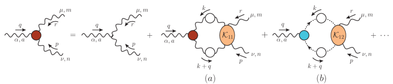
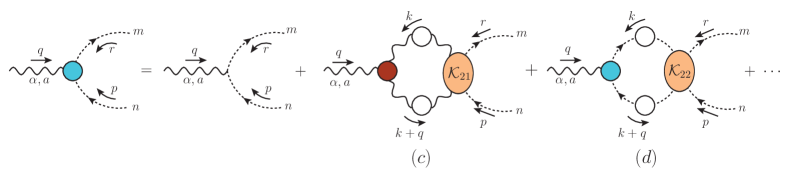
Figure 4: The coupled system of Schwinger-Dyson equations (SDEs) for the three-gluon and ghost-gluon vertices, ${\rm{I}}\!\Gamma_{\alpha\mu\nu}(q,r,p)$ and ${\rm{I}}\!\Gamma_{\alpha}(r,p,q)$, respectively. The orange ellipses represent four-point scattering kernels, denoted by ${\cal K}_{ij}$. We omit diagrams containing five-point scattering kernels.

The starting point for the derivations of the aforementioned BSEs are the SDEs for ${\rm{I}}\!\Gamma_{\alpha\mu\nu}(q,r,p)$ and ${\rm{I}}\!\Gamma_{\alpha}(r,p,q)$, shown diagrammatically in Fig. 4, and given by Aguilar et al. (2022)

$${\rm{I}}\!\Gamma^{\alpha\mu\nu} = \Gamma_{\!0}^{\alpha\mu\nu}-\lambda\int_{k}{\rm{I}}\!\Gamma^{\alpha\beta\gamma}\Delta_{\beta\rho}\Delta_{\gamma\sigma}{\cal K}_{11}^{\mu\nu\sigma\rho}+2\lambda\int_{k}{\rm{I}}\!\Gamma^{\alpha}DD{\cal K}_{12}^{\mu\nu}\,,$$

$${\rm{I}}\!\Gamma^{\alpha} = \Gamma_{\!0}^{\alpha}-\lambda\int_{k}{\rm{I}}\!\Gamma^{\alpha\beta\gamma}\Delta_{\beta\rho}\Delta_{\gamma\sigma}{\cal K}_{21}^{\sigma\rho}-\lambda\int_{k}{\rm{I}}\!\Gamma^{\alpha}DD{\cal K}_{22}\,,$$ (42)

where

$$\lambda:=ig^{2}C_{\rm A}/2\,,$$ (43)

and the tree-level expressions for the vertices ${\rm{I}}\!\Gamma^{\alpha\mu\nu}$ and ${\rm{I}}\!\Gamma^{\alpha}$ are given by

$$\Gamma_{\!0}^{\alpha\mu\nu}(q,r,p)=(q-r)^{\nu}g^{\alpha\mu}+(r-p)^{\alpha}g^{\mu\nu}+(p-q)^{\mu}g^{\nu\alpha}\,,\qquad\qquad\Gamma_{\!0}^{\alpha}(r,p,q)=r^{\alpha}\,.$$ (44)

Note that, for compactness, all momentum arguments have been suppressed; they may be easily restored by appealing to Fig. 4.

The following steps are subsequently implemented:

1. Substitute into both sides of Eq. (42) the expressions for the fully-dressed vertices given in Eq. (33).

2. In order to exploit Eq. (38), multiply the first equation by the factor ${P}_{\mu^{\prime}\mu}(r){P}^{\mu^{\prime}}_{\nu}(p)$.

3. Take the limit of the system as $q\to 0$: this activates Eq. (40) and introduces the functions ${\mathbb{C}}(r)$ and ${\mathbb{C}}(r)$.

4. Isolate the tensorial structures proportional to $q^{\alpha}$, and match the terms on both sides.

5. Employ the “one-particle exchange” approximation for the kernels ${\cal K}_{ij}$, to be denoted by ${\cal K}^{0}_{ij}$, shown in Fig. 5.

Thus, we arrive at a system of homogeneous equations involving ${\mathbb{C}}(r)$ and ${\mathcal{C}}(r)$,

$${\mathbb{C}}(r) = -\frac{\lambda}{3}\int_{k}{\mathbb{C}}(k)\Delta^{2}(k)P_{\rho\sigma}(k)P_{\mu\nu}(r)\widetilde{\cal K}_{11}^{\mu\nu\sigma\rho}+\frac{2\lambda}{3}\int_{k}{\mathcal{C}}(k)D^{2}(k)P_{\mu\nu}(r)\widetilde{\cal K}_{12}^{\mu\nu}\,,$$

$${\mathcal{C}}(r) = -\lambda\int_{k}{\mathbb{C}}(k)\Delta^{2}(k)P_{\sigma\rho}(k)\widetilde{\cal K}_{21}^{\sigma\rho}-\lambda\int_{k}{\mathcal{C}}(k)D^{2}(k)\widetilde{\cal K}_{22}\,,$$ (45)

where $\widetilde{\cal K}_{ij}:=(r\cdot k/r^{2})\,{\cal K}^{0}_{ij}(r,-r,k,-k)$; the system is diagrammatically depicted in Fig. 6.

Before turning to the numerical analysis, the BSE system must be passed to the Euclidean space, following standard conversion rules. In doing so we note that the integral measure is modified according to $d^{4}k\to id^{4}k_{{\scriptscriptstyle\rm E}}$; this extra factor of $i$ combines with the $\lambda$ defined in Eq. (43) to give real expressions.

As announced, the system of coupled equations given in Eq. (45) represents the BSEs that govern the formation of massless colored bound states out of two gluons and a ghost-antighost pair. The functions ${\mathbb{C}}(r)$ and ${\mathcal{C}}(r)$ are the corresponding BS amplitudes; finding nontrivial solutions for them, i.e., something other than ${\mathbb{C}}(r)={\mathcal{C}}(r)=0$ identically, is crucial for the implementation of the Schwinger mechanism.

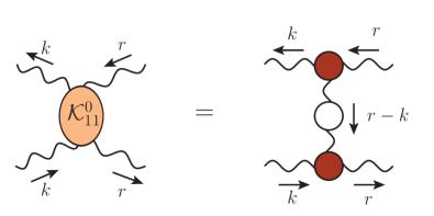
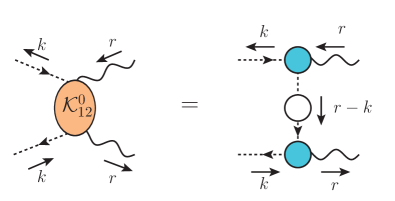
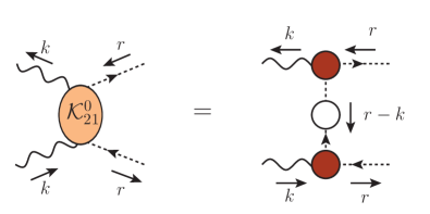
Figure 5: The one-particle exchange approximations, ${\cal K}^{0}_{ij}$, of the kernels ${\cal K}_{ij}$ appearing in Fig. 4.

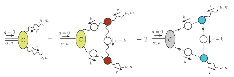
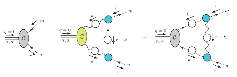
Figure 6: The diagrammatic representation of the coupled system of Bethe-Salpeter equations (BSEs) that governs the evolution of the functions ${\mathbb{C}}(r^{2})$ and ${\cal C}(r^{2})$.

The equations in Eq. (45) are linear and homogeneous in the unknown functions. There are two main consequences arising from this fact. First, the numerical solution of the system will be reduced to an eigenvalue problem. Second, the overall scale of the solutions is undetermined, since the multiplication of a given solution by an arbitrary real constant produces another solution .

It turns out that the condition for obtaining nontrivial solutions, when expressed in terms of the strong coupling, $\alpha_{s}:=g^{2}/4\pi$, states that they exist for $\alpha_{s}=0.63$, when the renormalization point $\mu=4.3$ GeV. The solutions obtained when $\alpha_{s}$ acquires this special value are shown in Fig. 7; they have undergone scale fixing, and are denoted by ${\mathbb{C}}_{\star}(r)$ and ${\mathcal{C}}_{\star}(r)$. Observe that ${\mathbb{C}}_{\star}(r)$ is significantly larger in magnitude than ${\mathcal{C}}_{\star}(r)$, implying that the three-gluon vertex accounts for the bulk of the gluon mass, as originally claimed in Aguilar et al. (2018).

It is important to compare the value of $\alpha_{s}=0.63$, imposed by the BSE eigenvalue, with the expected value for $\alpha_{s}$ for the renormalization scheme employed: within the asymmetric momentum subtraction (MOM) scheme (see Sec. 8), we have that $\alpha_{s}=0.27$ Boucaud et al. (2017). This numerical discrepancy in the values of $\alpha_{s}$ is clearly an artifact of the truncation employed, and concretely of the approximation of the kernels ${\cal K}_{ij}$ by their one-particle exchange diagrams, ${\cal K}^{0}_{ij}$. A preliminary analysis reveals that mild modifications of the kernels ${\cal K}_{ij}$ lead to considerable variations in the value of $\alpha_{s}$, but leave the form of the solutions for ${\mathbb{C}}_{\star}(r)$ and ${\mathcal{C}}_{\star}(r)$ practically unaltered. This observation suggests that, while a more complete knowledge of the BSE kernels is required in order to bring $\alpha_{s}$ closer to its MOM value, the solutions obtained with the present approximations should be considered as particularly stable.

Figure 7: The solutions for ${\mathbb{C}}_{\star}(r)$ (purple dot-dashed) and ${\mathcal{C}}_{\star}(r)$ (red dashed) obtained from the coupled BSE system of Eq. (45).

5 Generation of the gluon mass

We next demonstrate in detail how the presence of the massless poles in the vertices that enter in the SDE of the gluon propagator generate a gluon mass.

We start by pointing out that, since the fundamental STIs of the theory remain intact under the action of the Schwinger mechanism, Eqs. (7) and (8) remain valid, and the mass term $m^{2}=\Delta^{-1}(0)$ will appear in the transverse combination $\Delta^{-1}(0)P_{\mu\nu}(q)$. However, the determination of the mass proportional to $g_{\mu\nu}$ exposes an entirely different array of principles compared to the corresponding computation for the $q_{\mu}q_{\nu}/q^{2}$ component.

The calculation with respect to the $q_{\mu}q_{\nu}/q^{2}$ component is rather direct; since the massless poles in the vertices are themselves longitudinally coupled, their contribution to the $q_{\mu}q_{\nu}/q^{2}$ component of $\Pi_{\mu\nu}(q)$ is easily worked out, as will be illustrated in Subsec. 5.1. In contrast, the emergence of a mass proportional to $g_{\mu\nu}$ is intimately connected with a powerful relation, known as seagull identity Aguilar and Papavassiliou (2010); Aguilar et al. (2016), which in the absence of the Schwinger mechanism would enforce the masslessness of the propagator, as will be discussed in Subsec. 5.2. In fact, one main conceptual difference between the two approaches is that in the $g_{\mu\nu}$ case, the use of the PT-BFM-based version of the SDE given in Eq. (19) is crucial for the emergence of the correct result.

In order to simplify the technical aspects of the calculation without compromising its conceptual content, we will determine the contribution to the gluon mass due the pole in the ghost-gluon vertex, namely $V_{\alpha}(r,p,q)$ in the case of ${\rm{I}}\!\Gamma_{\alpha}(r,p,q)$, and $\widetilde{V}_{\alpha}(r,p,q)$ in the case of $\widetilde{{\rm{I}}\!\Gamma}_{\alpha}(r,p,q)$. To that end, we will focus on the subset of self-energy graphs containing only ghost loops, i.e., graph $(d_{3})$ in the case of $\Pi_{\mu\nu}(q)$, and graphs $(a_{3})$ and $(a_{4})$ in the case of $\widetilde{\Pi}_{\mu\nu}(q)$, shown in the upper and lower row of Fig. 1, respectively.

5.1 Gluon mass from the $q_{\mu}q_{\nu}$ component

Let us calculate the contribution to the gluon mass stemming from the ghost loop, i.e., the diagram $(d_{3})$ of Fig. 1, which, for general values of $q$, reads

$$(d_{3})_{\mu\nu}(q)=g^{2}C_{\rm A}\int_{k}(k+q)_{\mu}D(k+q)D(k){\rm{I}}\!\Gamma_{\nu}(-k,k+q,-q)\,.$$ (46)

To isolate the $q_{\mu}q_{\nu}/q^{2}$ component of Eq. (46) at the origin, we first decompose the full vertex ${\rm{I}}\!\Gamma_{\nu}(-k,k+q,-q)$ as in Eqs. (33) and (34), and drop directly the pole-free part, since it does not contribute at $q=0$. Then, denoting by $(d_{3}^{V})_{\mu\nu}(q)$ the contribution of $V_{\nu}(-k,k+q,-q)$ to $(d_{3})_{\mu\nu}(q)$, we obtain

$$(d_{3}^{V})_{\mu\nu}(q)=-g^{2}C_{\rm A}\frac{q_{\nu}}{q^{2}}\int_{k}(k+q)_{\mu}D(k+q)D(k)C(-k,k+q,-q)\,.$$ (47)

Next, a Taylor expansion around $q=0$, using Eqs. (39) and (40), yields

$$(d_{3}^{V})_{\mu\nu}(q)=-2g^{2}C_{\rm A}\frac{q_{\nu}q^{\rho}}{q^{2}}\int_{k}k_{\mu}k_{\rho}D^{2}(k){\mathcal{C}}(k)\,.$$ (48)

Evidently, the integral above can only be proportional to $g_{\mu\rho}$, such that

$$(d_{3}^{V})_{\mu\nu}(q)=-\frac{2g^{2}C_{\rm A}}{d}\left(\frac{q_{\mu}q_{\nu}}{q^{2}}\right)\int_{k}k^{2}D^{2}(k){\mathcal{C}}(k)\,,$$ (49)

where the tensor structure $q_{\mu}q_{\nu}/q^{2}$ is already isolated.

Then, let us denote by $\Delta^{-1}_{\rm gh}(0)$ the contribution to the mass originating in the $q_{\mu}q_{\nu}/q^{2}$ of the ghost loop. Noting that the contribution of $(d_{3}^{V})_{\mu\nu}(q)$ to the propagator is $i$ times the negative of its $q_{\mu}q_{\nu}/q^{2}$ form factor, we obtain that

$$\Delta^{-1}_{\rm gh}(0)=\frac{4\lambda}{d}\int_{k}k^{2}D^{2}(k){\mathcal{C}}(k)\,.$$ (50)

At this point, we set $d=4$ and renormalize Eq. (50). This leads to the appearance of the finite renormalization constant of the ghost-gluon vertex, $Z_{1}$.

Next, we express the result in terms of the ghost dressing function $F$, pass to Euclidean space, and employ hyperspherical coordinates, to obtain the final expression

$$\Delta^{-1}_{\rm gh}(0)=\hat{\lambda}\,Z_{1}\int_{0}^{\infty}\!\!dy\,F^{2}(y)\,{\cal C}(y)\,,$$ (51)

where $\hat{\lambda}:=C_{\mathrm{A}}\alpha_{s}/8\pi$.

The derivation of the contributions from the diagrams $(d_{1})$ and $(d_{4})$ proceeds in a completely analogous way, but is algebraically more involved, see Aguilar et al. (2016) for details.

It is instructive to consider how the result of Eq. (51) emerges in the context of Eq. (19). To this end, we consider the ghost block ${\widetilde{\Pi}}^{(2)}_{\mu\nu}(q)$ of Fig. 1, whose diagrams have the expressions given in Eq. (27); clearly, only diagram $(a_{3})_{\mu\nu}(q)$ can contribute to the $q_{\mu}q_{\nu}$ component of ${\widetilde{\Pi}}^{(2)}_{\mu\nu}(q)$.

Then, we decompose $\widetilde{\rm{I}}\!\Gamma_{\alpha}(r,p,q)$ in complete analogy with Eqs. (33) and (34), i.e.,

$$\widetilde{{\rm{I}}\!\Gamma}\vphantom{{\rm{I}}\!\Gamma}_{\alpha}(r,p,q)=\widetilde{\Gamma}_{\alpha}(r,p,q)+\frac{q_{\alpha}}{q^{2}}{\widetilde{C}}(r,p,q)\,,$$ (52)

and expand the $(a_{3})_{\mu\nu}(q)$ of Eq. (27) around $q=0$, isolating its $q_{\mu}q_{\nu}/q^{2}$ component. These steps eventually lead to

$${\widetilde{\Delta}}^{-1}_{\rm gh}(0)=\frac{4\lambda}{d}\int_{k}k^{2}D^{2}(k){\widetilde{\mathcal{C}}}(k)\,,$$ (53)

where ${\widetilde{\mathcal{C}}}(q)$ is defined in the exact same way as ${\mathcal{C}}(q)$, namely through Eq. (41) but with tildes over all relevant quantities. It is now easy to establish that Eq. (53) is completely equivalent to Eq. (50), simply by multiplying both of its sides by $Z_{1}F(0)$, and then using Eq. (131) on the r.h.s. and Eqs. (19) and (18) on the l.h.s.

Hence, when the mass is computed through the $q_{\mu}q_{\nu}/q^{2}$ component of the self-energy, the contributions originating from the ghost diagrams of either the BQ or the QQ propagator furnish the same result. The same is not true for the calculation through the $g_{\mu\nu}$ component, since the ghost diagram $(d_{3})_{\mu\nu}$ of the QQ propagator is not by itself transverse, and a meaningful analysis is preferably carried out within the BFM.

5.2 Gluon mass from the $g_{\mu\nu}$ component: seagull identity and Ward identity displacement

The fact that the activation of the Schwinger mechanism is crucial for the self-consistent generation of a gluon mass may be best appreciated in conjunction with the so-called seagull identity Aguilar and Papavassiliou (2010); Aguilar et al. (2016). The content of this identity is that

$$\int_{k}k^{2}\frac{\partial f(k)}{\partial k^{2}}+\frac{d}{2}\int_{k}\,f(k)=0\,,$$ (54)

for functions $f(k)$ that satisfy Wilson’s criterion Wilson (1973); the cases of physical interest are $f(k)=\Delta(k),D(k)$. The general demonstration of the validity of Eq. (54) has been given in Aguilar et al. (2016); for a detailed discussion of how Eq. (54) prevents the photon from acquiring a mass in scalar electrodynamics, see Aguilar et al. (2016).

What is so special about Eq. (54) is that, within the PT-BFM formalism, the l.h.s. of Eq. (54) coincides with the contributions of loop diagrams to the $g_{\mu\nu}$ component of the gluon mass. Therefore, Eq. (54) enforces the nonperturbative masslessness of the gluon in the absence of the Schwinger mechanism: even if a massive gluon propagator (made “massive” through a procedure other than the Schwinger mechanism) were to be substituted inside Eq. (54), one would obtain zero as contribution to the gluon mass! For example, the simple choice $f=(k^{2}-m^{2})^{-1}$, reduces the l.h.s of Eq. (54) to (dimensionally regularized) text-book integrals, which add up to give precisely zero Aguilar et al. (2016).

In order to appreciate in some detail how the seagull identity prevents the $g_{\mu\nu}$ component of the propagator from acquiring a mass in the absence of the Schwinger mechanism, let us consider once again the ghost block ${\widetilde{\Pi}}^{(2)}_{\mu\nu}(q)$ of Fig. 1; now both graphs, ($a_{3}$) and ($a_{4}$), contribute to the $g_{\mu\nu}$ component.

Let us assume that the Schwinger mechanism is turned off; at the level of the Bcc vertex this means that ${\widehat{V}}_{\alpha}(r,p,q)$ vanishes identically, and $\widetilde{{\rm{I}}\!\Gamma}\vphantom{{\rm{I}}\!\Gamma}_{\alpha}(r,p,q)=\widetilde{\Gamma}\vphantom{\Gamma}_{\alpha}(r,p,q)$. Consequently, $\widetilde{\Gamma}\vphantom{\Gamma}_{\alpha}(r,p,q)$ saturates the STI of Eq. (21),

$$q^{\alpha}\widetilde{\Gamma}\vphantom{\Gamma}_{\alpha}(r,p,q)={D}^{-1}(p)-{D}^{-1}(r)\,.$$ (55)

Since the form-factors of the vertex $\widetilde{\Gamma}\vphantom{\Gamma}_{\alpha}(r,p,q)$ do not contain any poles, the derivation from Eq. (55) of the corresponding WI proceeds in the standard text-book way: both sides of Eq. (55) undergo a Taylor expansion around $q=0$, and terms at most linear in $q$ are retained. Thus, one arrives at the simple QED-like WI

$${\widetilde{\Gamma}}_{\alpha}(r,-r,0)=\,\frac{\partial{D}^{-1}(r)}{\partial r^{\alpha}}\quad\Longrightarrow\quad D^{2}(r){\widetilde{\Gamma}}_{\alpha}(r,-r,0)=-2r_{\alpha}\frac{\partial{D}(r)}{\partial r^{2}}\,.$$ (56)

We now compute the $g_{\mu\nu}$ component of ${\widetilde{\Pi}}^{(2)}_{\mu\nu}(q)$ at $q=0$, or, equivalently, ${\widetilde{\Delta}}^{-1}_{\rm gh}(0)$. From Eq. (27), we see that $(a_{4})_{\mu\nu}$ is proportional to $g_{\mu\nu}$ in its entirety. On the other hand, $(a_{3})_{\mu\nu}(q)$ contains both $g_{\mu\nu}$ and $q_{\mu}q_{\nu}$ components; however, the latter vanishes in the limit $q\to 0$ if the vertex is pole-free. Then, it is straightforward to show that, as $q\to 0$,

$${\widetilde{\Delta}}^{-1}_{\rm gh}(0)=\frac{2\lambda}{d}\left[\int_{k}k_{\mu}D^{2}(k)\widetilde{\Gamma}^{\mu}(-k,k,0)+d\int_{k}D(k)\right]\,.$$ (57)

At this point, employing the WI of Eq. (56) (with $r\to-k$), we get

$${\widetilde{\Delta}}^{-1}_{\rm gh}(0)=\frac{4\lambda}{d}\underbrace{\left[\int_{k}k^{2}\frac{\partial{D}^{-1}(k)}{\partial k^{2}}+\frac{d}{2}\int_{k}D(k)\right]}_{\rm seagull\,\,identity}=0\,.$$ (58)

Hence, the WI satisfied by the vertex in the absence of the Schwinger mechanism triggers the seagull identity, which, in turn, enforces the masslessness of the propagator.

When the Schwinger mechanism gets activated, the STIs satisfied by the vertices of the theory retain their original form, but are resolved through the nontrivial participation of the terms containing the massless poles Eichten and Feinberg (1974); Poggio et al. (1975); Smit (1974); Cornwall (1982); Papavassiliou (1990); Aguilar et al. (2008); Binosi et al. (2012); Aguilar et al. (2016). In particular, the full vertex $\widetilde{{\rm{I}}\!\Gamma}\vphantom{{\rm{I}}\!\Gamma}_{\alpha}(r,p,q)$ satisfies precisely Eq. (21), namely

$$q^{\alpha}\widetilde{{\rm{I}}\!\Gamma}\vphantom{{\rm{I}}\!\Gamma}_{\alpha}(r,p,q) = q^{\alpha}\widetilde{\Gamma}_{\alpha}(r,p,q)+\widetilde{C}(r,p,q)$$ (59)

$$= {D}^{-1}(p)-{D}^{-1}(r)\,.$$

Notice in particular that the contraction of $\widetilde{{\rm{I}}\!\Gamma}\vphantom{{\rm{I}}\!\Gamma}_{\alpha}(r,p,q)$ by $q^{\alpha}$ cancels the massless pole in $q^{2}$, leading to a completely pole-free result. Therefore, the WI obeyed by $\widetilde{\Gamma}_{\alpha}(r,p,q)$ may be derived as before, through a standard Taylor expansion, leading to

$$q^{\alpha}\widetilde{\Gamma}_{\alpha}(r,-r,0)=-\widetilde{C}(r,-r,0)+q^{\alpha}\left\{\frac{\partial{D}^{-1}(r)}{\partial r^{\alpha}}-\left[\frac{\partial\widetilde{C}(r,p,q)}{\partial q^{\alpha}}\right]_{q=0}\right\}\,.$$ (60)

Evidently, the unique zeroth-order contribution appearing in Eq. (60), namely $\widetilde{C}(r,-r,0)$, must vanish,

$$\widetilde{C}(r,-r,0)=0\,.$$ (61)

Note that this particular property may be independently derived from the antisymmetry of $\widetilde{C}(r,p,q)$ under $r\leftrightarrow p$, $\widetilde{C}(r,p,q)=-\widetilde{C}(p,r,q)$, which is a consequence imposed by the ghost-antighost symmetry of the $B(q){\bar{c}}(r)c(p)$ vertex. The above result, together with Eq. (130), is used to prove Eq. (39) in App. A.

Thus, Eq. (60) becomes

$$q^{\alpha}\widetilde{\Gamma}_{\alpha}(r,-r,0)=q^{\alpha}\left\{\frac{\partial{D}^{-1}(r)}{\partial r^{\alpha}}-2r_{\alpha}{\widetilde{\mathcal{C}}}(r)\right\}\,,\qquad{\widetilde{\mathcal{C}}}(r):=\left[\frac{\partial{\widetilde{C}}(r,p,q)}{\partial p^{2}}\right]_{q=0}\,,$$ (62)

and the matching of the terms linear in $q$ yields the WI

$$\widetilde{\Gamma}_{\alpha}(r,-r,0)=\frac{\partial{D}^{-1}(r)}{\partial r^{\alpha}}-\underbrace{2r_{\alpha}\,{\widetilde{\mathcal{C}}}(r)}_{\rm WI\,displacement}\,.$$ (63)

Comparing Eqs. (56) and (63), it becomes clear that the Schwinger mechanism induces a characteristic displacement to the WIs that are satisfied by the pole-free parts of the vertices Aguilar et al. (2016).

Returning to Eq. (57), but now substituting in it the displaced version of Eq. (56), namely

$$D^{2}(k)\widetilde{\Gamma}^{\mu}(-k,k,0)=2k^{\mu}\left[\frac{\partial D(k)}{\partial k^{2}}+D^{2}(k)\widetilde{\cal C}(k)\right]\,.$$ (64)

When Eq. (64) is substituted into Eq. (57), the first term of its r.h.s. triggers the seagull identity and vanishes, exactly as before; however, the second term survives, furnishing precisely the result given in Eq. (53).

Completely analogous procedures may be applied to the remaining two blocks, ${\widetilde{\Pi}}^{(1)}_{\mu\nu}(q)$ and ${\widetilde{\Pi}}^{(3)}_{\mu\nu}(q)$, by exploiting the Abelian STIs of Eqs. (20) and (22), respectively Binosi et al. (2012).

6 Renormalization group invariant interaction strength

The PT-BFM formalism provides the natural framework for the construction of the RGI version of the naive one-gluon exchange interaction.

To fix the ideas, recall that in QED, the one-photon exchange interaction, defined as $\alpha\Delta_{\rm A}(q)$, where $\alpha:=e^{2}/4\pi$ is the hyper-fine structure constant and $\Delta_{\rm A}(q)$ the photon propagator, is an RGI combination, by virtue of the relation $Z_{e}=Z_{A}^{-1/2}$; see comments following Eq. (15). Moreover, this particular combination is universal (process-independent) because it may be identified within any two-to-two scattering process, regardless of the nature of the initial and final states (electrons, muons, taus, etc). Instead, in QCD, the corresponding combination $\alpha_{s}\Delta(q)$ is (trivially) universal but not RGI. When the vertices that connect the gluon to the external particles are “dressed” ($\Gamma_{0}\to\Gamma$), the combination $\Gamma\,\alpha_{s}\Delta\,\Gamma$   becomes RGI; however, it is no longer process-independent, because the vertices $\Gamma$ contain information on the characteristics of the external particles, e.g., the $\Gamma$ is not the same if the external particles are quarks or gluons. This apparent conundrum may be resolved by resorting to the PT, which reconciles harmoniously the notions of RGI and process-independence.

Within the PT framework, the starting point of the construction are “on-shell” processes Cornwall (1982); Cornwall and Papavassiliou (1989); Pilaftsis (1997); Binosi and Papavassiliou (2002, 2009), such as those depicted in Fig. 8. The fundamental observation is that the dressed vertices appearing there contain propagator-like contributions, which may be unambiguously identified by means of a well-defined diagrammatic procedure. After discarding terms that vanish on shell, the contributions extracted from a vertex have a two-fold effect: (i) the genuine vertex contributions left behind form a new vertex, $\widetilde{\Gamma}$, which satisfies Abelian STIs, and (ii) when the propagator-like pieces from both vertices are allotted to the conventional propagator, $\Delta_{\mu\nu}(q)$, the resulting effective propagator, $\widehat{\Delta}_{\mu\nu}(q)$, captures all RG logarithms associated with the running of the coupling; for example, at one loop and for large $q^{2}$, one has

$$\widehat{\Delta}^{-1}(q)\approx q^{2}\left[1+bg^{2}\ln(q^{2}/\mu^{2})\right]\,,$$ (65)

where $b=11C_{A}/48\pi^{2}$ is the first coefficient of the Yang-Mills $\beta$ function. We emphasize that the PT construction goes through to all orders in perturbation theory, as well as nonperturbatively, and all key properties of the PT Green’s function persist unaltered Binosi and Papavassiliou (2002, 2004).

The correspondence between the PT and the BFM may be summarized by stating that the PT rearrangement outlined above amounts effectively to replacing the Q-type gluon that is being exchanged (carrying momentum $q$) by a B-type gluon Denner et al. (1994); Hashimoto et al. (1994); Papavassiliou (1995); Pilaftsis (1997); external (on-shell) fields are always of the Q-type. Thus, the notation used above for the PT effective Green’s functions (“tildes” and “hats”) corresponds precisely to the BFM notation introduced in Section 2. Note that the formal expression of all PT rearrangements implemented diagrammatically are the BQIs that relate conventional Green’s functions to their BFM counterparts Binosi and Papavassiliou (2009). For example, in the case of the quark-gluon vertex, we have that the vertices ${\mathbf{\Gamma}}_{\mu}(q,k_{1},-k_{2})$ [with external fields $Q^{a}_{\mu}(q)q^{b}(k_{1}){\bar{q}}^{c}(-k_{2})$] and ${\widetilde{\mathbf{\Gamma}}}_{\mu}(q,k_{1},-k_{2})$ [$B^{a}_{\mu}(q)q^{b}(k_{1}){\bar{q}}^{c}(-k_{2})$] are related by the BQI Aguilar et al. (2014)

$${\widetilde{\mathbf{\Gamma}}}_{\mu}(q,k_{1},-k_{2})=[1+G(q)]{\mathbf{\Gamma}}_{\mu}(q,k_{1},-k_{2})+\cdots\,,$$ (66)

where the ellipsis denotes terms that vanish on shell. Similarly, the BQI of Eq. (A), when evaluated on-shell, yields a completely analogous result, to wit,

$$\widetilde{{\rm{I}}\!\Gamma}\vphantom{{\rm{I}}\!\Gamma}_{\mu\alpha\rho}(q,k_{1},-k_{2})=[1+G(q)]{\rm{I}}\!\Gamma_{\mu\alpha\rho}(q,k_{1},-k_{2})+\cdots\,.$$ (67)

It is now clear how the PT gives rise to a process-independent propagator-like component: regardless of the process (i.e., the type of vertex connecting the internal gluon to the external states), each vertex contributes to the conventional $\Delta(q)$ a factor of $[1+G(q)]^{-1}$, finally leading to the BQI of Eq. (11) Binosi et al. (2015).

The culmination of the above sequence of ideas is reached by noting that, by virtue of Eq. (15), the combination

$${\widehat{d}}(q):=\alpha_{s}{\widehat{\Delta}(q)}=\frac{\alpha_{s}\Delta(q)}{[1+G(q)]^{2}}\,,$$ (68)

is RGI: it retains exactly the same form before and after renormalization, and, consequently, does not depend on the renormalization point $\mu$ Cornwall (1982). The quantity ${\widehat{d}}(q)$ has mass dimension of $-2$, and is known in the literature as the “RGI running interaction strength” Binosi et al. (2015).

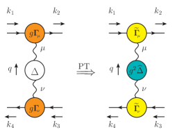
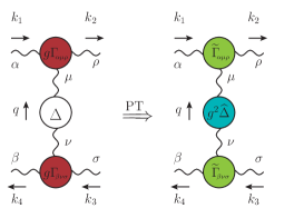
Figure 8: Diagrammatic representation of the basic PT rearrangement in the case of quark-antiquark scattering, corresponding to the S-matrix element ${\cal T}_{q{\bar{q}}\to q{\bar{q}}}$ of Eq. (69)   (left), and gluon-gluon scattering, corresponding to ${\cal T}_{gg\to gg}$ of Eq. (70)   (right).

The steps leading to the natural appearance of ${\widehat{d}}(q)$ within any given process may be summarized in the case of quark-antiquark, or gluon-gluon scattering.

Consider the S-matrix elements ${\cal T}_{q{\bar{q}}\to q{\bar{q}}}$, for the scattering of a quark and an antiquark, and ${\cal T}_{gg\to gg}$, for the scattering of two gluons. The quark-antiquark scattering is depicted in the left panel of Fig. 8. Using the BQI of Eq. (11) we obtain

$${\cal T}_{q{\bar{q}}\to q{\bar{q}}}= \,\,\left[g{\mathbf{\Gamma}}_{\mu}(q,k_{1},-k_{2})\right]\Delta(q)P^{\mu\nu}(q)\left[g{\mathbf{\Gamma}}_{\nu}(-q,k_{3},-k_{4})\right]$$

$$\overset{{\rm PT}}{=} \,\,\left\{g[1+G(q)]^{-1}{\widetilde{\mathbf{\Gamma}}}_{\mu}(q,k_{1},-k_{2})\right\}\Delta(q)P^{\mu\nu}(q)\left\{g[1+G(q)]^{-1}{\widetilde{\mathbf{\Gamma}}}_{\nu}(-q,k_{3},-k_{4})\right\}$$

$$\overset{{\rm PT}}{=} \,\,{\widetilde{\mathbf{\Gamma}}}_{\mu}(q,k_{1},-k_{2})\left\{g^{2}[1+G(q)]^{-2}\Delta(q)\right\}P^{\mu\nu}(q){\widetilde{\mathbf{\Gamma}}}_{\nu}(-q,k_{3},-k_{4})$$

$$\overset{{\rm PT}}{=} \,\,{\widetilde{\mathbf{\Gamma}}}_{\mu}(q,k_{1},-k_{2})\underbrace{\left[g^{2}{\widehat{\Delta}}(q)\right]}_{4\pi{\widehat{d}}(q)}P^{\mu\nu}(q){\widetilde{\mathbf{\Gamma}}}_{\nu}(-q,k_{3},-k_{4})\,,$$ (69)

where we omit color structures.

Similarly, the scattering of two gluons, depicted in the right panel of Fig. 8, yields

$${\cal T}_{gg\to gg}= \,\,\left[g\Gamma_{\alpha\mu\rho}(k_{1},q,-k_{2})\right]\Delta(q)P^{\mu\nu}(q)\left[g\Gamma_{\beta\nu\sigma}(k_{3},-q,-k_{4})\right]$$

$$\overset{{\rm PT}}{=} \,\,\left\{g[1+G(q)]^{-1}{\widetilde{\Gamma}}_{\alpha\mu\rho}(k_{1},q,-k_{2})\right\}\Delta(q)P^{\mu\nu}(q)\left\{g[1+G(q)]^{-1}{\widetilde{\Gamma}}_{\beta\nu\sigma}(k_{3},-q,-k_{4})\right\}$$

$$\overset{{\rm PT}}{=} \,\,{\widetilde{\Gamma}}_{\alpha\mu\rho}(k_{1},q,-k_{2})\left\{g^{2}[1+G(q)]^{-2}\Delta(q)\right\}P^{\mu\nu}(q){\widetilde{\Gamma}}_{\beta\nu\sigma}(k_{3},-q,-k_{4})$$

$$\overset{{\rm PT}}{=} \,\,{\widetilde{\Gamma}}_{\alpha\mu\rho}(k_{1},q,-k_{2})\underbrace{\left[g^{2}{\widehat{\Delta}}(q)\right]}_{4\pi{\widehat{d}}(k)}P^{\mu\nu}(q){\widetilde{\Gamma}}_{\beta\nu\sigma}(k_{3},-q,-k_{4})\,.$$ (70)

Evidently, the same ${\widehat{d}}(q)$, defined in Eq. (68), appears naturally in both Eqs. (69) and (70): it is, in that sense, a process-independent RGI interaction capturing faithfully the one-gluon exchange dynamics Cornwall (1982); Watson (1997); Binosi and Papavassiliou (2003); Aguilar et al. (2009); Binosi et al. (2015, 2017); Cui et al. (2020); Roberts (2020).

The actual determination of ${\widehat{d}}(q)$ proceeds by means of the second equality in Eq. (68), i.e., by combining the standard gluon propagator, $\Delta(q)$, together with the function $1+G(q)$. In the top left panel of Fig. 9 we show lattice data for the conventional gluon propagator from Aguilar et al. (2021b) (points) and a physically motivated fit (blue continuous), given by Eq. (C11) of Aguilar et al. (2022). In the top right panel of the same figure we show the $1+G(q)$ auxiliary function, which can be computed by contracting Eq. (12) with $P^{\mu\nu}(q)/3$ (see, e.g.,  Aguilar et al. (2009)), using the results of Aguilar et al. (2019) for the ghost-gluon kernel, $H_{\nu\mu}(r,p,q)$. Then, in the bottom left panel of Fig. 9 we show the ${\widehat{d}}(q)$ that results from combining the fit for $\Delta(q)$ and the $1+G(q)$ shown in the top panels of the same figure and using $\alpha_{s}=0.27$ Boucaud et al. (2017) and $Z_{1}=0.9333$ [see Sec. 8].

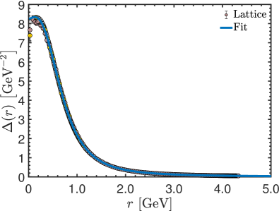
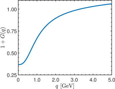
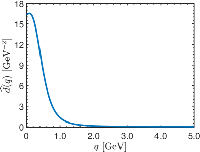
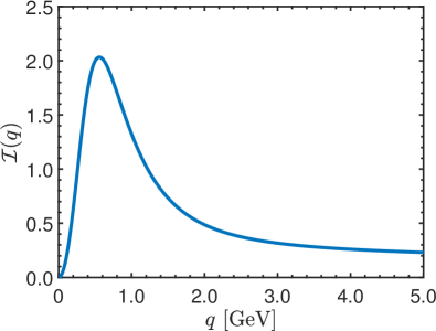
Figure 9: Top left: Gluon propagator, $\Delta(q)$, from lattice simulations of Ref. Aguilar et al. (2021b) (points) and a fit given by Eq. (C11) of Aguilar et al. (2022) (blue continuous). Top right: The auxiliary function $1+G(q)$, defined in Eq. (12). Bottom left: The renormalization group invariant (RGI) running interaction strength ${\widehat{d}}(q)$ defined in Eq. (68), computed using the $\Delta(q)$ and $1+G(q)$ shown in the top panels, with $\alpha_{s}=0.27$ Boucaud et al. (2017) and $Z_{1}=0.9333$ [see Sec. 8]. Bottom right: The corresponding dimensionless RGI interaction ${\cal I}(q)$, defined in Eq. (71).

From the ${\widehat{d}}(q)$ of Eq. (68) one may define the dimensionless RGI interaction Binosi et al. (2015), ${\cal I}(q)$,

$${\cal I}(q):=q^{2}{\widehat{d}}(q)\,.$$ (71)

As explained in Binosi et al. (2015), this quantity provides the strength required in order to describe ground-state hadron observables using SDEs in the matter sector of the theory. In that sense, ${\cal I}(q)$ bridges a longstanding gap that has existed between nonperturbative continuum QCD and ab initio predictions of basic hadron properties.

7 Three-gluon vertex and its planar degeneracy

The three-gluon vertex, ${\rm{I}}\!\Gamma_{\alpha\mu\nu}(q,r,p)$, plays a pivotal role in the dynamics of QCD Papavassiliou et al. (2022), manifesting its non-Abelian nature through the gluon self-interaction. In fact, the most celebrated perturbative feature of QCD, namely asymptotic freedom, hinges on the properties of this particular interaction vertex. Its importance in the nonperturbative domain has led to an intense effort for unveiling its elaborate features Alkofer et al. (2005); Pelaez et al. (2013); Aguilar et al. (2014); Blum et al. (2014); Eichmann et al. (2014); Williams et al. (2016); Blum et al. (2015); Cyrol et al. (2016); Corell et al. (2018); Boucaud et al. (2017); Huber (2020); Aguilar et al. (2019, 2020, 2019); Parrinello (1994); Alles et al. (1997); Parrinello et al. (1998); Boucaud et al. (1998); Cucchieri et al. (2006, 2008); Athenodorou et al. (2016); Duarte et al. (2016); Boucaud et al. (2017); Vujinovic and Mendes (2019); Aguilar et al. (2019); Barrios et al. (2022); Pinto-Gómez et al. (2022); Pinto-Gomez and de Soto (2022). Indeed, as we have seen in Secs. 3 and 4, the pole structure of the three-gluon vertex is crucial for the onset of the Schwinger mechanism and the dynamical generation of a gluon mass. Moreover, its pole-free part provides highly nontrivial contributions to the SDEs of several Green’s functions, most notably the gluon propagator (cf. Fig. 1), as well as in the Bethe-Salpeter and Faddeev equations that determine the properties of glueballs Meyers and Swanson (2013); Sanchis-Alepuz et al. (2015); Souza et al. (2020); Huber et al. (2020, 2021) and hybrid mesons Xu et al. (2019), respectively.

For general momenta, ${\rm{I}}\!\Gamma_{\alpha\mu\nu}(q,r,p)$ is a particularly complicated function, comprised by 14 tensor structures and their associated form factors Ball and Chiu (1980). Fortunately, in the Landau gauge, considerable simplifications take place, making the treatment of the three-gluon vertex less cumbersome. Indeed, in the latter gauge, quantities of interest require only the knowledge of the transversely projected three-gluon vertex Eichmann et al. (2014); Blum et al. (2014); Huber (2016); Aguilar et al. (2022), $\overline{\Gamma}\vphantom{\Gamma}_{\alpha\mu\nu}(q,r,p)$, defined as

$$\overline{\Gamma}\vphantom{\Gamma}_{\alpha\mu\nu}(q,r,p) ={\rm{I}}\!\Gamma^{\alpha^{\prime}\mu^{\prime}\nu^{\prime}}(q,r,p)P_{\alpha^{\prime}\alpha}(q)P_{\mu^{\prime}\mu}(r)P_{\nu^{\prime}\nu}(p)$$

$$=\Gamma^{\alpha^{\prime}\mu^{\prime}\nu^{\prime}}(q,r,p)P_{\alpha^{\prime}\alpha}(q)P_{\mu^{\prime}\mu}(r)P_{\nu^{\prime}\nu}(p)\,.$$ (72)

Note that $\overline{\Gamma}\vphantom{\Gamma}_{\alpha\mu\nu}(q,r,p)$ does not contain massless poles, by virtue of Eq. (35). Furthermore, $\overline{\Gamma}\vphantom{\Gamma}_{\alpha\mu\nu}(q,r,p)$ can be parametrized in terms of only $4$ independent tensor structures, i.e.,

$$\overline{\Gamma}\vphantom{\Gamma}^{\alpha\mu\nu}(q,r,p)=\sum_{i=1}^{4}\widetilde{\Gamma}_{i}(q^{2},r^{2},p^{2})\,\mkern 2.0mu\widetilde{\mkern-4.0mu\lambda\mkern-2.0mu}\mkern 1.2mu_{i}^{\alpha\mu\nu}(q,r,p)\,.$$ (73)

Due to the Bose symmetry of $\overline{\Gamma}\vphantom{\Gamma}_{\alpha\mu\nu}(q,r,p)$, the $\mkern 2.0mu\widetilde{\mkern-4.0mu\lambda\mkern-2.0mu}\mkern 1.2mu_{i}^{\alpha\mu\nu}(q,r,p)$ can be chosen to be individually Bose symmetric, such that its form factors $\widetilde{\Gamma}_{i}(q^{2},r^{2},p^{2})$ are symmetric under the exchange of any two arguments Pinto-Gómez et al. (2022). In fact, they can only depend on three totally symmetric combinations of momenta.

Quite remarkably, lattice Pinto-Gómez et al. (2022); Pinto-Gomez and de Soto (2022); Pinto-Gómez et al. (2022) and continuum Eichmann et al. (2014); Blum et al. (2014); Huber (2016) studies alike, have demonstrated that, to a very good level of accuracy, the $\widetilde{\Gamma}_{i}$ depend exclusively on a single judiciously chosen variable. Specifically, the $\widetilde{\Gamma}_{i}$ computed on the lattice in Pinto-Gómez et al. (2022); Pinto-Gomez and de Soto (2022); Pinto-Gómez et al. (2022) can be parametrized in terms of the special Bose symmetric combination

$$s^{2}=\frac{1}{2}\left(q^{2}+r^{2}+p^{2}\right)\,.$$ (74)

Thus, the $\widetilde{\Gamma}_{i}$ are the same for any combination of $q^{2}$, $r^{2}$, and $p^{2}$ that fulfils Eq. (74) for a given value of $s^{2}$. This property has been denominated planar degeneracy, because Eq. (74) with fixed $s$ defines a plane, normal to the vector $(1,1,1)$, in the first octant of the coordinate system $(q^{2},r^{2},p^{2})$.

In particular, the form factor $\widetilde{\Gamma}_{1}(q^{2},r^{2},p^{2})$ of the classical tensor structure is rather accurately approximated by

$$\widetilde{\Gamma}_{1}(q^{2},r^{2},p^{2})\approx\widetilde{\Gamma}_{1}(s^{2},s^{2},0)\approx\mathit{L}_{{sg}}(s)\,.$$ (75)

In the above equation, $\mathit{L}_{{sg}}$ is the single transverse form factor of the three-gluon vertex in the soft gluon limit Aguilar et al. (2022), and is obtained in lattice simulations as the $q=0$ limit of the following totally transverse projection Aguilar et al. (2021a)

$$\mathit{L}_{{sg}}(r)=\left.\frac{\Gamma_{0}^{\alpha\mu\nu}(q,r,p)P_{\alpha\alpha^{\prime}}(q)P_{\mu\mu^{\prime}}(r)P_{\nu\nu^{\prime}}(p){\rm{I}}\!\Gamma^{\alpha^{\prime}\mu^{\prime}\nu^{\prime}}(q,r,p)}{\Gamma_{0}^{\alpha\mu\nu}(q,r,p)P_{\alpha\alpha^{\prime}}(q)P_{\mu\mu^{\prime}}(r)P_{\nu\nu^{\prime}}(p)\Gamma_{0}^{\alpha^{\prime}\mu^{\prime}\nu^{\prime}}(q,r,p)}\right|_{q\to 0}\,.$$ (76)

A particular realization of the planar degeneracy property is shown in Fig. 10, where we show the classical form factor $\widetilde{\Gamma}_{1}(q^{2},r^{2},p^{2})$, obtained from the lattice simulation of Pinto-Gómez et al. (2022); we consider three different kinematic configurations, characterized by a single momentum. Specifically, the orange stars correspond to the soft-gluon limit, $q=0$, which implies $p^{2}=r^{2}$; the green diamonds denote the symmetric limit, where all of the momenta have the same magnitude, $q^{2}=p^{2}=r^{2}$; and the purple circles represent points with $p^{2}=r^{2}$ and $q^{2}=2r^{2}$. When plotted against the momentum $r$, the three configurations of $\widetilde{\Gamma}_{1}(q^{2},r^{2},p^{2})$ produce three clearly distinct curves; however, when plotted in terms of the Bose symmetric variable $s$ of Eq. (74), they become statistically indistinguishable, manifesting the validity of Eq. (75).

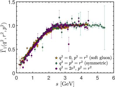
Figure 10: Lattice data from Ref. Pinto-Gómez et al. (2022) for the classical form factor, $\widetilde{\Gamma}_{1}(q^{2},r^{2},p^{2})$, of the transversely projected three-gluon vertex in three different kinematic configurations: the soft-gluon ($q=0$, $p^{2}=r^{2}$, orange stars), the symmetric limit ($q^{2}=p^{2}=r^{2}$, green diamonds), and the case $p^{2}=r^{2}$ with $q^{2}=2r^{2}$ (purple circles). In the left panel $\widetilde{\Gamma}_{1}(q^{2},r^{2},p^{2})$ is plotted as a function of $r$, while in the right it is plotted as a function of the Bose symmetric variable $s$ defined in Eq. (74).

In addition to the planar degeneracy property, lattice Aguilar et al. (2021a); Pinto-Gómez et al. (2022); Pinto-Gomez and de Soto (2022); Pinto-Gómez et al. (2022) and continuum Eichmann et al. (2014); Blum et al. (2014); Huber (2016); Aguilar et al. (2019) results show a clear dominance of the classical form factor $\widetilde{\Gamma}_{1}$ over the remaining ones. Based on these considerations, the special approximation

$$\overline{\Gamma}\vphantom{\Gamma}^{\alpha\mu\nu}(q,r,p)\approx L_{\textrm{sg}}\left(s\right){\overline{\Gamma}}_{\!0}^{\alpha\mu\nu}(q,r,p)\,,$$ (77)

has been put forth, where ${\overline{\Gamma}}_{\!0}^{\alpha\mu\nu}(q,r,p)$ is the tree-level value of $\overline{\Gamma}\vphantom{\Gamma}^{\alpha\mu\nu}(q,r,p)$, i.e., Eq. (7) with $\Gamma^{\alpha^{\prime}\mu^{\prime}\nu^{\prime}}(q,r,p)\to{\Gamma}^{\alpha^{\prime}\mu^{\prime}\nu^{\prime}}_{\!0}(q,r,p)$. Eq. (77) provides an accurate and exceptionally compact approximation for $\overline{\Gamma}\vphantom{\Gamma}^{\alpha\mu\nu}(q,r,p)$ in general kinematics.

We emphasize that the shape of $\mathit{L}_{{sg}}(r)$ has been very precisely determined through dedicated lattice studies with large-volume simulations Athenodorou et al. (2016); Boucaud et al. (2017); Aguilar et al. (2021a, b). The outcome of this exploration is shown in Fig. 11, where we plot the lattice data of Aguilar et al. (2021a) for $\mathit{L}_{{sg}}(r)$, together with a physically motivated fit given by Eq. (C12) of Aguilar et al. (2022) (blue continuous curve).

The approximation given by Eq. (77), with the fit for $\mathit{L}_{{sg}}$ shown in Fig. 11, will be used explicitly in Secs. 8 and 11, where the $\overline{\Gamma}\vphantom{\Gamma}^{\alpha\mu\nu}(q,r,p)$ in general kinematics will be needed as input for the determination of other physically important quantities.

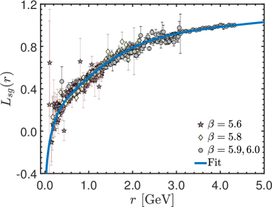
Figure 11: Lattice data from Ref. Aguilar et al. (2021a) for $\mathit{L}_{{sg}}(q)$, compared to the fit for it given by Eq. (C12) of Aguilar et al. (2022) (blue continuous curve).

8 Ghost dynamics from Schwinger-Dyson equations

We next turn our attention to the ghost sector of the theory, whose scrutiny is important for several reasons. First, it has been connected to particular scenarios of color confinement Kugo and Ojima (1979); Nakanishi and Ojima (1990). Second, the Green’s functions associated with the ghost sector appear as ingredients in the SDEs of several key functions, such as the gluon propagator and the three-gluon vertex Cucchieri et al. (2006, 2008); Alkofer et al. (2010); Aguilar et al. (2014); Pelaez et al. (2013); Blum et al. (2014); Eichmann et al. (2014); Williams et al. (2016); Blum et al. (2015); Cyrol et al. (2016); Duarte et al. (2016); Athenodorou et al. (2016); Boucaud et al. (2017); Aguilar et al. (2019, 2020, 2019), affecting their nonperturbative behavior in nontrivial ways, as will be discussed in Sec. 9. Third, the SDEs governing the ghost sector are simpler than their gluonic counterparts, because they are comprised by fewer diagrams; in fact, the SDE of the ghost propagator contains a single diagram, see Fig. 12. Fourth, in the Landau gauge, the validity of Taylor’s theorem Taylor (1971) facilitates considerably the task of renormalization.

Consequently, the SDEs of the ghost sector are an excellent testing ground for $(a)$ probing the impact of the gluonic Green’s functions that contribute to them Aguilar et al. (2021b); $(b)$ assessing the reliability of truncation schemes Huber (2017); Aguilar et al. (2022); and $(c)$ testing the agreement between lattice and continuum approaches.

One of the central results of numerous studies in the continuum  Aguilar et al. (2008); Dudal et al. (2008); Boucaud et al. (2008, 2008); Kondo (2010); Boucaud et al. (2012); Pennington and Wilson (2011); Dudal et al. (2012); Aguilar et al. (2013); Cyrol et al. (2016); Huber (2020); Aguilar et al. (2019, 2021b) as well as a variety of lattice simulations Ilgenfritz et al. (2007); Cucchieri and Mendes (2007); Bogolubsky et al. (2007); Cucchieri and Mendes (2008); Bogolubsky et al. (2009); Ayala et al. (2012); Boucaud et al. (2018); Cui et al. (2020) may be summarized by stating that the ghost propagator, $D(q)$, remains massless, while the corresponding dressing function, $F(q)$, saturates at the origin. As we will discuss in Sec. 9, the nonperturbative masslessness of the ghost has important implications for the infrared behavior of the gluon propagator and the three-gluon vertex.

In what follows we provide a concrete example of the state-of-the-art SDE analysis of the ghost sector, by solving the coupled system of equations that governs the ghost-dressing function and the ghost-gluon vertex. In order to obtain a closed system of equations, we use lattice results for the gluon propagator, the three-gluon vertex, and the value of the coupling constant in the particular renormalization scheme employed.

The main points of this analysis may be summarized as follows.

(i) We begin by considering the coupled system of SDEs given by Fig. 12, which determines the ghost propagator and ghost-gluon vertex. The treatment will be simplified by neglecting diagram $(d_{3}^{\nu})$ of Fig. 12, thus eliminating the dependence on the ghost-ghost-gluon-gluon vertex, $\Gamma^{\mu\sigma}$. This is a particularly robust truncation, because the impact of the neglected diagram on the ghost-gluon vertex has been shown to be less than $2\%$ Huber (2017).

(ii) Note that due to the fully transverse nature of the gluon propagators in the Landau gauge, in conjunction with the fact that various projections need to be implemented during the treatment of this system, the pole parts $V$ of all fully dressed vertices appearing in Fig. 12 will be annihilated; thus, we will have throughout the replacement ${\rm{I}}\!\Gamma\to\Gamma$.

(iii) We proceed by decomposing the pole-free part, $\Gamma_{\nu}(r,q,p)$, of the ghost-gluon vertex into its most general Lorentz structure, namely

$$\Gamma_{\nu}(r,q,p)=r_{\nu}B_{1}(r,q,p)+p_{\nu}B_{2}(r,q,p)\,,$$ (78)

whose scalar form factors reduce to $B_{1}^{0}=1$ and $B_{2}^{0}=0$ at tree level. Evidently, due to the transversality of the gluon propagator, only the classical tensor $r_{\nu}$, accompanied by the form factor $B_{1}$, will survive in all SDE diagrams of Fig. 12.

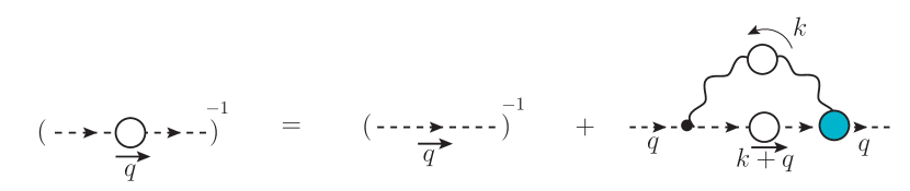
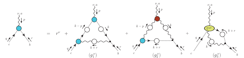
Figure 12: Top: SDE governing the momentum evolution of the ghost propagator. Bottom: SDE for the ghost-gluon vertex, ${\rm{I}}\!\Gamma_{\nu}(r,q,p)$.

(iv) The SDE of Fig. 12 is given by

$$F^{-1}(r)=1+2\lambda\int_{k}f(k,r)B_{1}(-r,k+r,-k)\Delta(k)D(k+r)\,,$$ (79)

where $\lambda$ is given by Eq. (43), and we define

$$f(k,r):=1-\frac{(r\cdot k)^{2}}{r^{2}k^{2}}\,.$$ (80)

(v) Next, we note that the form factor $B_{1}(r,q,p)$ can be extracted from $\Gamma_{\nu}(r,q,p)$ through the projection

$$B_{1}(r,q,p)=\varepsilon^{\nu}\Gamma_{\nu}(r,q,p)\,,\qquad\varepsilon^{\nu}:=\frac{p^{2}r^{\nu}-(r\cdot p)p^{\nu}}{r^{2}p^{2}-(r\cdot p)^{2}}\,.$$ (81)

Hence, acting with $\varepsilon^{\nu}$ on the diagrams in the second line of Fig. 12, we obtain

$$B_{1}(r,q,p)=1-\lambda\left[a(r,q,p)-b(r,q,p)\right]\,,$$ (82)

where

$$a(r,q,p) =q^{\alpha}r^{\mu}\varepsilon^{\nu}\!\!\int_{k}D(k)D(k-p)\Delta(k+r)B_{1}(p-k,q,k+r)B_{1}(-k,k-p,p)P_{\alpha\mu}(k+r)k_{\nu}\,,$$

$$b(r,q,p) =q^{\alpha}r^{\mu}\varepsilon^{\nu}\!\!\int_{k}\Delta(k)\Delta(k-p)D(k+r)B_{1}(k+r,q,p-k)\overline{\Gamma}\vphantom{\Gamma}_{\nu\mu\alpha}(p,-k,k-p)\,.$$ (83)

(vi) At this point, we invoke the property of the planar degeneracy of $\overline{\Gamma}\vphantom{\Gamma}_{\alpha\mu\nu}(q,r,p)$, discussed in Sec. 7. Employing Eq. (77) into the SDE for $B_{1}$, the term $b(r,q,p)$ of Eq. (83) becomes

$$b(r,q,p)=q^{\alpha}r^{\mu}\varepsilon^{\nu}\!\!\int_{k}\Delta(k)\Delta(k-p)D(k+r)B_{1}(k+r,q,p-k)\overline{\Gamma}\vphantom{\Gamma}^{0}_{\nu\mu\alpha}(p,-k,k-p)\mathit{L}_{{sg}}({\bar{s}})\,,$$ (84)

with ${\bar{s}}^{2}=p^{2}+k^{2}-2(k\cdot p)$.

We emphasize that although Eq. (77) constitutes in general an approximation, there is one particular kinematic limit in which the expression for $b(r,q,p)$ given in Eq. (84) becomes exact. Specifically, in the soft gluon limit ($p=0$), it can be shown exactly that Aguilar et al. (2021b)

$$P_{\mu}^{\mu^{\prime}}(k)P_{\nu}^{\nu^{\prime}}(k)\Gamma_{\alpha\mu^{\prime}\nu^{\prime}}(0,k,-k)=2\mathit{L}_{{sg}}(k)k_{\alpha}P_{\mu\nu}(k)\,.$$ (85)

Then, starting from either the general expression for $b(r,q,p)$ of Eq. (83) and using Eq. (85), or from the approximate version given by Eq. (84), it can easily be shown that the $p=0$ limit is the same. As such, the use of Eq. (77) yields not only an excellent approximation in general kinematics, but also the exact soft gluon limit for the contribution of the three-gluon vertex to the form factor $B_{1}$.

(vii) Now we consider the renormalization of the coupled system of equations. Since the ghost-gluon vertex is finite in the Landau gauge Taylor (1971), most SDE treatments Schleifenbaum et al. (2005); Boucaud et al. (2008); Huber and von Smekal (2013); Aguilar et al. (2013, 2019, 2021b) of the ghost sector employ the so-called Taylor renormalization scheme, defined in such a way that the finite renormalization constant of the ghost-gluon vertex has the exact value $Z_{1}=1$ Taylor (1971); Boucaud et al. (2009); Blossier et al. (2010); Zafeiropoulos et al. (2019); Aguilar et al. (2021b).

However, in order to employ Eq. (77) most expeditiously, it is more convenient to renormalize in the so-called asymmetric MOM scheme, because this is precisely the scheme employed in the lattice calculations of $\mathit{L}_{{sg}}$ Athenodorou et al. (2016); Boucaud et al. (2017); Aguilar et al. (2021a, b). Specifically, this scheme is defined by imposing the normalization conditions Aguilar et al. (2021a, b)

$$\Delta^{-1}_{{\rm{\scriptscriptstyle R}}}(\mu)=\mu^{2}\,,\qquad F_{{\rm{\scriptscriptstyle R}}}(\mu)=1\,,\qquad\mathit{L}_{{sg}}^{{\rm{\scriptscriptstyle R}}}(\mu)=1\,.$$ (86)

Past this point, we denote by ${\widetilde{Z}}_{1}$ the finite value of the ghost-gluon renormalization constant in the asymmetric MOM scheme. Evidently, Eqs. (14) and (78) imply that $B_{1}^{{\rm{\scriptscriptstyle R}}}={\widetilde{Z}}_{1}B_{1}$.

The renormalization of Eqs. (79) and (82) proceeds by substitution of the unrenormalized quantities by their renormalized counterparts, following Eq. (14), and imposing Eq. (86) for $F(\mu^{2})$.

Note that, in principle, ${\widetilde{Z}}_{1}$, may be determined from the relation ${\widetilde{Z}}_{1}=Z_{3}Z_{c}Z_{A}^{-1}$, imposed by the corresponding STI Celmaster and Gonsalves (1979); however, these renormalization constants are not available to us, given that the associated Green’s functions have been obtained from the lattice. Therefore, ${\widetilde{Z}}_{1}$ is treated as an adjustable parameter, whose value is determined by requiring that the solution of the SDE for $F(q)$ reproduces the corresponding lattice data of Boucaud et al. (2018); Aguilar et al. (2021b) as well as possible.

(viii) Finally, we transform Eqs. (79) and (82) from Minkowski to Euclidean space, using standard conversion rules. Note that, once in Euclidean space, we will express the functional dependence of $B_{1}(r,q,p)$ in terms of the squared momenta of the antighost and gluon legs, $r^{2}$ and $p^{2}$, and the angle, $\theta$, between them, i.e., $B_{1}(r,q,p)\equiv B_{1}(r^{2},p^{2},\theta)$.

The result of these manipulations is that Eqs. (79) and (82) become

$$F^{-1}(r) =1-\frac{\alpha_{s}C_{\rm A}{\widetilde{Z}}_{1}}{2\pi^{2}}\int_{0}^{\infty}dk^{2}k^{2}\Delta(k)\int_{0}^{\pi}d\phi\,s_{\phi}^{4}$$

$$\times\left[B_{1}(r^{2},k^{2},\phi)\frac{F(\sqrt{z})}{z}-B_{1}(\mu^{2},k^{2},\phi)\frac{F(\sqrt{u})}{u}\right]\,,$$ (87)

and

$$B_{1}(r^{2},p^{2},\theta)={\widetilde{Z}}_{1}-\frac{\alpha_{s}C_{\rm A}{\widetilde{Z}}_{1}}{8\pi^{2}}\left[{\overline{a}}+2{\overline{b}}\right]\,,$$ (88)

respectively, with

$${\overline{a}} =\frac{1}{s_{\theta}}\int_{0}^{\infty}dk^{2}k^{2}F(k)\int_{0}^{\pi}d\phi s_{\phi}^{3}\frac{\Delta(\sqrt{z})}{z}\int_{0}^{\pi}d\omega s_{\omega}\frac{F(\sqrt{v})}{v}B_{1}(k^{2},p^{2},\alpha)B_{1}(v,z,\beta){\cal K}_{a}\,,$$ (89)

$${\overline{b}} =\frac{1}{s_{\theta}}\int_{0}^{\infty}dk^{2}k^{2}\Delta(k)\int_{0}^{\pi}d\phi s_{\phi}^{3}\frac{F(\sqrt{z})}{z}\int_{0}^{\pi}d\omega s_{\omega}\frac{\Delta(\sqrt{v})}{v}B_{1}(z,v,\beta)\mathit{L}_{{sg}}({\overline{s}}){\cal K}_{b}\,.$$

In the above equations we employ the notation $c_{x}:=\cos x$ and $s_{x}:=\sin x$, and define the following variables

$$r\cdot k:=rkc_{\phi}\,, p\cdot k:=pk(c_{\theta}c_{\phi}+s_{\theta}s_{\phi}c_{\omega})\,,$$

$$z:=r^{2}+k^{2}+2rkc_{\phi}\,, u:=\mu^{2}+k^{2}+2\mu kc_{\phi}\,,$$

$${\overline{s}}^{2}:=(p^{2}+k^{2}+v)/2\,, v:=p^{2}+k^{2}-2pk(c_{\theta}c_{\phi}+s_{\theta}s_{\phi}c_{\omega})\,,$$

$$\alpha:=\pi-\cos^{-1}\left[c_{\theta}c_{\phi}+s_{\theta}s_{\phi}c_{\omega}\right]\,, \beta:=\cos^{-1}\left[\frac{k(pc_{\theta}c_{\phi}+ps_{\theta}s_{\phi}c_{\omega}-rc_{\phi})+prc_{\theta}-k^{2}}{\sqrt{vz}}\right]\,.$$

Finally, the kernels ${\cal K}_{a}$ and ${\cal K}_{b}$ are given by

$${\cal K}_{a}= (c_{\theta}c_{\omega}s_{\phi}-c_{\phi}s_{\theta})\left[ks_{\phi}(pc_{\theta}+r)-pc_{\theta}c_{\omega}(kc_{\phi}+r)\right]\,,$$

$${\cal K}_{b}= c_{\omega}\left\{k^{2}pc_{\phi}\left[c_{\theta}p\left(s_{\theta}^{2}(s_{\phi}^{2}s_{\omega}^{2}-4s_{\phi}^{2}+1)+s_{\phi}^{2}\right)+r\left(s_{\phi}^{2}-s_{\theta}^{2}(2s_{\phi}^{2}+1)\right)\right]\right.$$

$$-k^{3}\left[s_{\phi}^{2}\left(rc_{\theta}-2ps_{\theta}^{2}+p\right)+ps_{\theta}^{2}\right]+kp^{2}\left[s_{\phi}^{2}\left(2s_{\theta}^{2}(p-rc_{\theta})-rc_{\theta}-p\right)+s_{\theta}^{2}(rc_{\theta}-p)\right]$$

$$\left.\left.-c_{\phi}p^{3}rs_{\theta}^{2}\right\}+s_{\theta}s_{\phi}\left\{c_{\theta}p\left[r\left(p^{2}-k^{2}(s_{\omega}^{2}+s_{\phi}^{2}s_{\omega}^{2}-2s_{\phi}^{2})\right)-c_{\phi}k(s_{\omega}^{2}-2)(k^{2}+p^{2})\right]\right.\right.$$

$$+k\left[c_{\phi}k^{2}r-c_{\phi}p^{2}r\left(s_{\theta}^{2}(s_{\omega}^{2}-2)+s_{\omega}^{2}\right)+kp^{2}\left(3s_{\theta}^{2}s_{\phi}^{2}s_{\omega}^{2}-2s_{\theta}^{2}s_{\omega}^{2}-4s_{\theta}^{2}s_{\phi}^{2}+3s_{\theta}^{2}\right.\right.$$

$$\left.\left.\left.+(3-2s_{\omega}^{2})s_{\phi}^{2}-2\right)\right]\right\}\,.$$

We are now in position to solve Eqs. (87) and (88) numerically. We choose the renormalization point at $\mu=4.3$ GeV, and employ for $\Delta(q)$ and $\mathit{L}_{{sg}}(q)$ the fits to lattice data shown in Figs. 9 and 11, respectively. Note that for large momenta these fits recover the behavior dictated by the corresponding anomalous dimensions Aguilar et al. (2022). For the strong coupling, we use the value $\alpha_{s}(4.3\text{ GeV})=0.27$, determined from the lattice simulations of Boucaud et al. (2017).

Below we discuss the main results of this analysis:

The value of ${\widetilde{Z}}_{1}$ was obtained by solving the SDE system for various values of this constant until the $\chi^{2}$ of the comparison between the solution for $F(q)$ and the lattice data of Boucaud et al. (2018); Aguilar et al. (2021b) was minimized. This procedure yields ${\widetilde{Z}}_{1}=0.9333\pm 0.0075$.

In the left panel of Fig. 13 we show as a blue continuous line the SDE result for $F(q)$, with the above value of ${\widetilde{Z}}_{1}$. The result is compared to the lattice data of Boucaud et al. (2018); Aguilar et al. (2021b), which have been cured from discretization artifacts. As it turns out, the SDE and lattice results for $F$ agree within $1\%$.

We next consider the form factor $B_{1}$. In the right panel of Fig. 13 we show $B_{1}(r^{2},p^{2},\theta)$ as a surface, for arbitrary values of the magnitudes of the momenta $r$ and $p$, and for the angle $\theta$ formed between them at $\theta=2\pi/3$. In the same panel, we highlight as a red dot-dashed curve the soft gluon limit $B_{1}(r^{2},0,2\pi/3)$ of the general kinematics $B_{1}(r^{2},p^{2},2\pi/3)$.

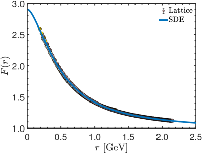
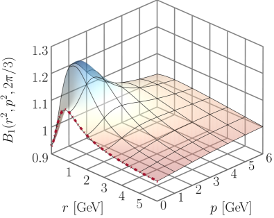
Figure 13: Left: ghost dressing function $F(q)$ obtained from the coupled system of SDEs of Eqs. (79) and (82) (blue continuous line) compared to the lattice data of Ref. Boucaud et al. (2018); Aguilar et al. (2021b). Right: The corresponding result for $B_{1}(r^{2},p^{2},\theta)$ for arbitrary magnitudes of the antighost and gluon momenta, $r$ and $p$, respectively, and a representative value of $\theta=2\pi/3$ for the angle between them. The red dot-dashed curve highlights the soft gluon limit ($p=0$).

The only available SU(3) lattice data for $B_{1}$ have been obtained in the soft gluon limit Ilgenfritz et al. (2007); Sternbeck (2006), and have sizable error bars. Furthermore, they have been computed within the Taylor scheme, while in the present work we used the asymmetric MOM scheme. Nevertheless, we can meaningfully compare our SDE results with those of the lattice, and perform a statistical analysis to assess their agreement.

Specifically, denoting by $B_{1}^{\rm{\scriptscriptstyle T}}$ the Taylor scheme value of the form factor $B_{1}$, it can easily be shown that

$$B_{1}(r^{2},p^{2},\theta)={\widetilde{Z}}_{1}B_{1}^{\rm{\scriptscriptstyle T}}(r^{2},p^{2},\theta)\,,$$ (90)

which allows us to carry out the desired comparison.

Then, we use Eq. (90) to compute $B_{1}^{\rm{\scriptscriptstyle T}}(r^{2},0,\theta)$ from the $B_{1}(r^{2},0,2\pi/3)$ slice (red dot-dashed curve) in the right panel of Fig. 13, and compare the result to the lattice data of Ilgenfritz et al. (2007); Sternbeck (2006) (points) in Fig. 14. Evidently, the SDE determination agrees with the lattice results.

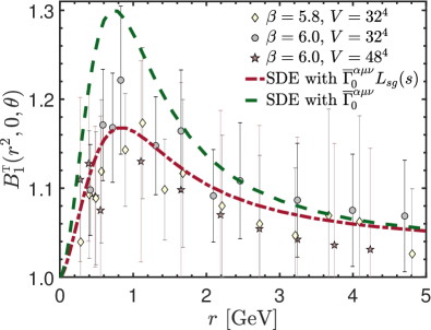
Figure 14: Soft gluon limit, $B_{1}^{\rm{\scriptscriptstyle T}}(r^{2},0,\theta)$, of the classical form factor of the ghost-gluon vertex in Taylor scheme. The points correspond to the lattice data of Ref. Ilgenfritz et al. (2007); Sternbeck (2006). The red dot-dashed line shows the SDE solution with the three-gluon vertex dressed according to Eq. (77), while the green dashed represents the SDE solution with tree-level three-gluon vertex.

In order to quantify this agreement, we next conduct a $\chi^{2}$ analysis. To this end, we consider only the 22 lattice points $r_{i}$ in the interval $r_{i}\in[0.3,2.5]$ GeV, where the signal is most pronounced. Then, we compute the $\chi^{2}$ of the data through

$$\chi^{2}_{j}=\sum_{i}\frac{[B_{1}^{\rm lat}(r_{i}^{2},0,\theta)-g_{j}(r_{i})]^{2}}{\epsilon_{B_{1}}(r_{i}^{2},0,\theta)}\,,$$ (91)

where $B_{1}^{\rm lat}(r_{i}^{2},0,\theta)$ are the lattice points shown in Fig. 14, $\epsilon_{B_{1}}(r_{i}^{2},0,\theta)$ their respective errors, and $g_{j}(r_{i})$ are three hypotheses which we will compare to the lattice data. Specifically, for the $g_{j}$ we consider the three cases

$$g_{j}(r_{i})=\begin{cases}1&\text{if }j=1\,,\\ \text{SDE with }\overline{\Gamma}\vphantom{\Gamma}^{\alpha\mu\nu}={\overline{\Gamma}}_{\!0}^{\alpha\mu\nu}\mathit{L}_{{sg}}(s)&\text{if }j=2\,,\\ \text{SDE with }\overline{\Gamma}\vphantom{\Gamma}^{\alpha\mu\nu}={\overline{\Gamma}}_{\!0}^{\alpha\mu\nu}&\text{if }j=3\,,\end{cases}$$ (92)

i.e., $g_{1}$ is the tree-level value of $B_{1}$, $g_{2}$ the solution of the SDE using Eq. (77) for dressing the three-gluon vertex, corresponding to the red dot-dashed curve of Fig. 14, and $g_{3}$ is the solution of the SDE obtained setting the three-gluon vertex to tree-level, which amounts to the substitution $\mathit{L}_{{sg}}\to 1$ in Eq. (88), and is represented by a green dashed curve in Fig. 14.

Then, for each $\chi_{j}^{2}$ we compute the probability $P_{j}$ that normally distributed errors would yield a $\chi^{2}$ at least as large as $\chi_{j}^{2}$, through

$$P_{j}=\int_{\chi^{2}_{j}}^{\infty}\chi_{\rm{\scriptscriptstyle PDF}}^{2}(22,x)dx=\left.\frac{\Gamma(n_{r}/2,\chi^{2}/2)}{\Gamma(n_{r}/2)}\right|_{n_{r}=22}^{\chi^{2}=\chi^{2}_{j}}\,.$$ (93)

In the above equation, $\chi_{\rm{\scriptscriptstyle PDF}}^{2}(n,x)=x^{n/2-1}e^{-x/2}/[2^{n/2}\Gamma(n/2)]$ denotes the $\chi^{2}$ probability distribution function with $n$ degrees of freedom, while $\Gamma(z,x)$ is the incomplete $\Gamma$ function.

The results of the above analyses are collected in Table 2. We note that the case $g_{1}$, i.e., the tree-level value of $B_{1}$, is discarded at $5.1\sigma$ confidence level. As for case $g_{3}$, it is discarded at the $3.4\sigma$ level. On the other hand, the SDE result with dressed three-gluon vertex, $g_{2}$, is statistically indistinguishable from the lattice data.

Table 2: Statistical results of the $\chi^{2}$ analysis for the three hypotheses given in Eq. (92) for the form factor $B_{1}$. For each case (first column), we give the corresponding $\chi^{2}_{j}$ computed from Eq. (91) (second column), probability $P_{j}$ computed from Eq. (93) (third row), and the same $P_{j}$ expressed in terms of confidence levels $\sigma$ (fourth row).

Case ($j$)	$\chi^{2}_{j}$	$P_{j}$	Confidence level in $\sigma$
1	71.37	$4.0\times 10^{-7}$	$5.1$
2	3.399	1 - $1.8\times 10^{-6}$	$2.2\times 10^{-6}$
3	50.03	$5.8\times 10^{-4}$	$3.4$

Lastly, we point out that for both $F$ and $B_{1}$ we find a good qualitative agreement with various related studies Schleifenbaum et al. (2005); Huber and von Smekal (2013); Aguilar et al. (2013); Cyrol et al. (2016); Mintz et al. (2018); Aguilar et al. (2019); Huber (2020); Aguilar et al. (2019); Huber (2020); Barrios et al. (2020), including kinematics other than the soft gluon limit considered in Fig. 14.

9 Divergent ghost loops and their impact on the QCD Green’s functions

The masslessness of the ghost propagator, discussed in Sec. 8, has important implications for the infrared behavior of other Green’s functions. Specifically, while the saturation of the gluon propagator renders gluon loops infrared finite, ghost loops furnish infrared divergent contributions Aguilar et al. (2014), akin to those encountered in perturbation theory. In this section, we highlight with two characteristic examples how the effects of ghost loops manifest themselves at the level of the two- and three-point functions. Specifically, the ghost loops induce the appearance of a moderate maximum in the gluon propagator and are responsible for the zero-crossing and the logarithmic divergence at the origin displayed by the dominant form factors of the three-gluon vertex.

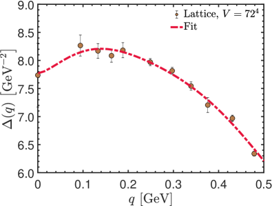
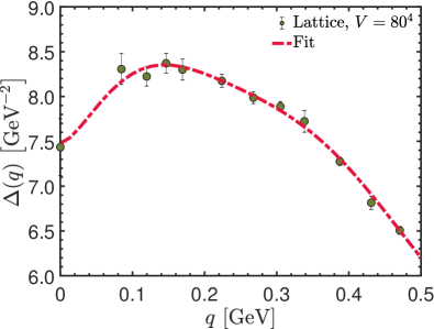
Figure 15: Lattice data for the gluon propagator in the deep infrared. The data displayed correspond to the two lattice setups with the largest volumes of Bogolubsky et al. (2007), namely, $V=72^{4}$ (left) and $V=80^{4}$ (right). The red dashed lines are smooth fits from which the position of the maximum can be estimated.

The basic observation at the level of the gluon SDE shown in Fig. 1 is that, the ghost loop of $(d_{3})$, due to the masslessness of its ingredients, furnishes “unprotected” logarithms, i.e., terms of the type $\ln q^{2}$, which diverge as $q^{2}\to 0$. Instead, gluonic loops contain infrared finite gluon propagators, and, therefore, give rise to contributions that remain finite as $q^{2}\to 0$, i.e., they may be described in terms of “protected” logarithms of the type $\ln(q^{2}+m^{2})$.

The circumstances described above may be modeled by

$$\Delta^{-1}(q)=\underbrace{q^{2}+m^{2}+c_{1}q^{2}\ln\left(\frac{q^{2}+\rho m^{2}}{\Lambda^{2}}\right)}_{f(q)}+c_{2}q^{2}\ln\left(\frac{q^{2}}{\Lambda^{2}}\right)\,,$$ (94)

where $m$ is the gluon mass, $\Lambda$ the mass scale of QCD, and $c_{1}$, $c_{2}$ and $\rho$ are constants; note that $\Delta^{-1}(0)=f(0)=m^{2}$

Differentiating Eq. (94) with respect to $q^{2}$ we obtain

$$\frac{d\Delta^{-1}(q)}{dq^{2}}=\frac{df(q)}{dq^{2}}+c_{2}\left[1+\ln\left(\frac{q^{2}}{\Lambda^{2}}\right)\right]\,.$$ (95)

The second term on the r.h.s. of Eq. (95) is infrared divergent, and necessarily dominates the behavior of the derivative of the propagator for sufficiently small $q$. Moreover, the value of the coefficient $c_{2}$ can be computed explicitly by expanding the ghost block ${\widetilde{\Pi}}^{(2)}_{\mu\nu}(q)$ of Fig. 1 around $q=0$ and using Eq. (19), which yields

$$c_{2}=\frac{\alpha_{s}C_{\rm A}{\widetilde{Z}}_{1}^{2}F^{2}(0)}{48\pi}\,.$$ (96)

Therefore, $d\Delta^{-1}(q)/dq^{2}$ has the asymptotic behavior

$$\lim_{q\to 0}\frac{d\Delta^{-1}(q)}{dq^{2}}=\left[\frac{\alpha_{s}C_{\rm A}{\widetilde{Z}}_{1}^{2}F^{2}(0)}{48\pi}\right]\ln\left(\frac{q^{2}}{\Lambda^{2}}\right)\,,$$ (97)

which diverges to $-\infty$ as $q\to 0$. Now, since the gluon propagator is a decreasing function in the ultraviolet, we have that $d\Delta^{-1}(q)/dq^{2}$ is positive for large momenta. Therefore, there must exist a special momentum, denoted by $q_{\star}$, such that $[d\Delta(q)/dq^{2}]_{q=q_{\star}}=0$, which corresponds to a maximum of $\Delta(q)$.

The maximum of $\Delta(q)$, predicted by means of the simple arguments presented above, is observed in lattice simulations of the gluon propagator Bogolubsky et al. (2007, 2009); Aguilar et al. (2021b). In particular, it is clearly visible in Fig. 15, where the data from the two largest volume lattice setups of Bogolubsky et al. (2007) are shown. The red dashed lines represent smooth functions, fitted to each of the data sets, in the window $q\in[0,0.5]$ GeV. For each of the volumes considered, $V=72^{4}$ (left panel) and $V=80^{4}$ (right panel), the estimate obtained for $q_{\star}$ is $q_{\star}=140$ MeV.

It is interesting to observe in passing that the existence of a maximum of $\Delta(q)$ has an interesting implication on the form of the spectral function of the gluon propagator Cyrol et al. (2018); Binosi and Tripolt (2020); Kern et al. (2019); Horak et al. (2021, 2022a, 2022b). In particular, the standard Källén-Lehmann representation Kallen (1952); Lehmann (1954) states that

$$\Delta(q)=\int_{0}^{\infty}\!\!d\lambda^{2}\,\frac{\rho(\lambda^{2})}{q^{2}+\lambda^{2}}\,,$$ (98)

where $\rho(\lambda^{2})$ is the gluon spectral function (with a factor $1/\pi$ absorbed in it). Thus, the differentiation of both sides of Eq. (98) with respect to $q^{2}$ yields

$$\frac{d\Delta(q)}{dq^{2}}=-\int_{0}^{\infty}\!\!d\lambda^{2}\,\frac{\rho(\lambda^{2})}{(q^{2}+\lambda^{2})^{2}}\,.$$ (99)

Then, from Eq. (99) follows that the existence of a maximum for $\Delta(q)$ at $q=q_{\star}$ leads necessarily to the violation of reflection positivity Osterwalder and Schrader (1973, 1975); Alkofer and von Smekal (2001); Cornwall (2013), because the condition

$$\int_{0}^{\infty}\!\!d\lambda^{2}\,\frac{\rho(\lambda^{2})}{(q^{2}_{\star}+\lambda^{2})^{2}}=0\,,$$ (100)

may be fulfilled only if $\rho(\lambda^{2})$ reverses its sign. Note that an analogous argument based on the existence of an inflection point has been presented recently in Ding et al. (2022).

Turning to the three-gluon vertex, it is well known that the corresponding ghost loops induce characteristic features to the form factors associated with its classical (tree-level) tensors. There are two complementary continuum descriptions of the dynamics that determine the behavior of these form factors: ${(\it i)}$ the SDE of the three-gluon vertex Huber and von Smekal (2013); Blum et al. (2014); Eichmann et al. (2014); Williams et al. (2016), depicted diagrammatically in Fig. 16, and ${(\it ii)}$ the STI of Eq. (23) Aguilar et al. (2014), which, in the limit of vanishing gluon momentum, and when the displacement function and the ghost sector are neglected, yields the approximate WI

$${{\rm{I}}\!\Gamma}_{\alpha\mu\nu}(0,r,-r)\approx\frac{\partial\Delta^{-1}_{\mu\nu}(r)}{\partial r^{\alpha}}\,,$$ (101)

which transmits the properties of the propagator derivative to the vertex form factors, as shown schematically in Fig. 18.

In the simplified kinematic circumstances where only a single representative momentum is considered, to be denoted by $r$, the conclusions drawn by either method may be qualitatively described in terms of a simple model, namely

$$L(r)=b_{0}+b_{\rm gl}\ln\left(\frac{r^{2}+m^{2}}{\Lambda^{2}}\right)+b_{\rm gh}\ln\left(\frac{r^{2}}{\Lambda^{2}}\right)\,,$$ (102)

where $L(r)$ denotes the particular combination of form factors, such that, at tree level, $L_{0}(r)=1$, and $b_{0}$, $b_{\rm gl}$, and $b_{\rm gh}$ are positive constants. The model in Eq. (102) encompasses two important cases studied on the lattice Athenodorou et al. (2016); Duarte et al. (2016); Boucaud et al. (2017); Aguilar et al. (2020), namely ${(\it i)}$ the soft gluon limit, $L(r)\to\mathit{L}_{{sg}}(r)$, corresponding to the kinematic choice $q\to 0\,,\quad p=-r\,,\quad\theta:=\widehat{pr}=\pi$, defined in Eq. (76), and ${(\it ii)}$ totally symmetric limit, $L(r)\to L_{sym}(r)$, corresponding to $q^{2}=p^{2}=r^{2}\,,\quad\theta:=\widehat{qr}=\widehat{qp}=\widehat{rp}=2\pi/3$.

Upon inspection of Eq. (102) we note that, as $r\to 0$, the term with the unprotected logarithm will eventually dominate, forcing $L(r)$ to reverse its sign (zero crossing), and finally display a logarithmic divergence, $L(0)\to-\infty$. Given that, in practice, $b_{\rm gl}$ is considerably larger than $b_{\rm gh}$, the unprotected logarithm overtakes the protected one rather deep in the infrared: the location of the zero-crossing is at about $160$ MeV Boucaud et al. (2017). Consequently, in the intermediate region of momenta, which is considered relevant for the onset of nonperturbative dynamics, we have $L(r)<1$; this effect is known in the literature as the infrared suppression of the three-gluon vertex.

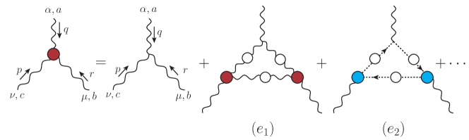
Figure 16: The SDE of the three-gluon vertex at the one-loop dressed level. The diagrams $(e_{1})$ and $(e_{2})$ are the gluon and the ghost triangle contributions entering in the skeleton expansion of the three-gluon vertex.

Most importantly, the special features of infrared suppression, zero-crossing, and logarithmic divergence at the origin have been corroborated through a variety of lattice results Cucchieri et al. (2008); Athenodorou et al. (2016); Duarte et al. (2016); Boucaud et al. (2017); Sternbeck et al. (2017); Aguilar et al. (2020, 2021a), as shown, e.g., in Fig. 11. The central curve of this figure is presented as the blue line in Fig. 17, where the aforementioned characteristics have been explicitly marked for the benefit of the reader. Note the close proximity of the blue curve to the $d\Delta^{-1}(r)/dr^{2}$ (red dashed line), especially below 1 GeV.

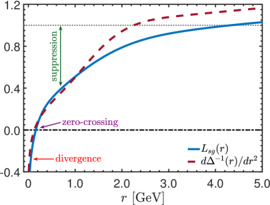
Figure 17: Comparison of $\mathit{L}_{{sg}}(r)$ (blue continuous) from Fig. 11 and $d\Delta^{-1}(r)/dr^{2}$ (red dashed) resulting from the fit for $\Delta(r)$ of Fig. 9. Note that both display the characteristic features of infrared suppression with respect to their tree-level values (which is $1$ for both quantities), zero-crossing, and logarithmic divergence at the origin.

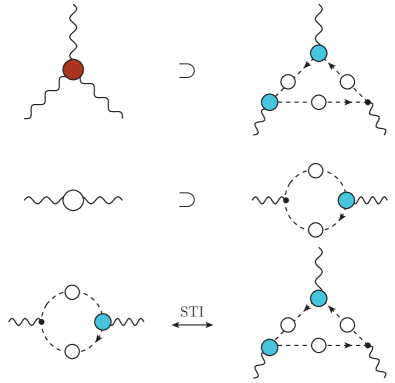
Figure 18: The ghost triangle present in the three-gluon vertex SDE (top) and the ghost loop contributing to the gluon propagator in the corresponding equation (middle). The infrared divergences arising from these diagrams are connected through the Slavnov-Taylor identity (STI) of Eq. (23), as shown schematically in the bottom panel.

We end this section by pointing out that, in the case of Yang-Mills in $d=3$ Gross et al. (1981); Jackiw and Templeton (1981); Appelquist and Pisarski (1981); Deser et al. (1982); Cornwall (1989, 1994); Alexanian and Nair (1995); Cornwall and Yan (1996); Cornwall (1996); Buchmuller and Philipsen (1997); Jackiw and Pi (1997); Cornwall (1998); Karabali et al. (1998); Eberlein (1998); Aguilar et al. (2010, 2014); Huber (2016); Corell et al. (2018), the situation is qualitatively similar to the one described above, but the divergences induced due to the masslessness of the ghost are stronger. Specifically, as may be already established at the level of a simple one-loop calculation  Aguilar et al. (2010), the first derivative of the gluon propagator diverges at the origin as $1/q$ rather than a $\ln q^{2}$. Consequently, the corresponding effects are significantly enhanced; in particular, the maximum of the gluon propagator is considerably more pronounced, becoming plainly visible on the lattice Cucchieri and Mendes (2009). Similarly, an abrupt negative divergence is observed in the corresponding vertex form factors Cucchieri et al. (2006); Maas and Vujinović (2022).

10 Ward identity displacement of the three-gluon vertex

In complete analogy to the case of the ghost-gluon vertex discussed in subsection 5.2, the WI satisfied by the pole-free part of the three-gluon vertex is also displaced in the presence of longitudinally coupled massless poles. Quite importantly, the associated displacement function, ${\mathbb{C}}(r)$, coincides with the BS amplitude that controls the formation of a (colored) scalar bound state with vanishing mass out of a gluon pair. The displacement of the WI circumvents the seagull cancellation involving the gluon propagator [i.e., $f=\Delta$ in Eq. (54)], furnishing to the $g_{\mu\nu}$ component the mass originating from graphs $(d_{1})$ and $(d_{4})$ in Fig. 1. In addition, it permits the indirect determination of the displacement function ${\mathbb{C}}(r)$ from the lattice; this is particularly important, given that, by virtue of Eq. (35), the lattice “observables” do not perceive directly the presence of the massless poles.

The starting point of the analysis is the STI satisfied by the three-gluon vertex, ${\rm{I}}\!\Gamma_{\alpha\mu\nu}(q,r,p)$, given by Eq. (23). In order to eliminate the poles in $r$ and $p$, thus isolating the displacement of the WI originating from the pole in the channel $q$, we contract that equation with $P_{\mu^{\prime}}^{\mu}(r)P_{\nu^{\prime}}^{\nu}(p)$. Note that this procedure also eliminates any longitudinal pole terms in the $H_{\sigma\mu}(p,q,r)$ and $H_{\sigma\nu}(r,q,p)$.

Then, we decompose ${\rm{I}}\!\Gamma_{\alpha\mu\nu}(q,r,p)$ into pole-free and longitudinally coupled massless pole parts, as in Eq. (33), and use Eq. (38), to obtain

$$P_{\mu^{\prime}}^{\mu}(r)P_{\nu^{\prime}}^{\nu}(p)\left[q^{\alpha}\Gamma_{\alpha\mu\nu}(q,r,p)+g_{\mu\nu}C_{1}(q,r,p)+q_{\mu}q_{\nu}C_{5}(q,r,p)\right]=P_{\mu^{\prime}}^{\mu}(r)P_{\nu^{\prime}}^{\nu}(p)R_{\nu\mu}(p,q,r)\,,$$ (103)

where

$$R_{\nu\mu}(p,q,r):=F(q)\left[\Delta^{-1}(p)P_{\nu}^{\sigma}(p)H_{\sigma\mu}(p,q,r)-\Delta^{-1}(r)P_{\mu}^{\sigma}(r)H_{\sigma\nu}(r,q,p)\right]\,.$$ (104)

At this point, we expand Eq. (103) around $q=0$ and match coefficients of equal orders. At zeroth order in this expansion we obtain immediately that

$$C_{1}(0,r,-r)=0\,,$$ (105)

in exact analogy to Eq. (61). Note that we have arrived once again at the result of Eq. (39), but through an entirely different path: while Eq. (39) is enforced by the Bose symmetry of the three-gluon vertex, Eq. (105) is a direct consequence of the STI that this vertex satisfies.

We next gather the terms in the expansion of Eq. (103) that are of first order in $q$. Evidently, the term $C_{5}$ does not contribute to this order. Then, the expansion leads to the appearance of derivatives of the gluon propagator, in analogy to Eq. (63), but also of the ghost-gluon kernel. Specifically, we obtain for the WI of the three-gluon vertex and its displacement the expression

$$\mathit{L}_{{sg}}(r)=F(0)\left\{\widetilde{Z}_{1}\frac{d\Delta^{-1}(r)}{dr^{2}}+\frac{{\cal W}(r)}{r^{2}}\Delta^{-1}(r)\right\}-{\mathbb{C}}(r)\,.$$ (106)

In the above equation, $\mathit{L}_{{sg}}(r)$ is the form factor of the three-gluon vertex defined in Eq. (76) and with lattice results shown in Fig. 11, while ${\cal W}(r)$ is a particular derivative of the ghost-gluon kernel, namely Aguilar et al. (2020, 2022)

$${\cal W}(r)=-\frac{1}{3r^{2}}P^{\mu\nu}(r)\left[\frac{\partial H_{\nu\mu}(p,q,r)}{\partial q^{\alpha}}\right]_{q=0}\,.$$ (107)

For the detailed derivation of Eq. (106), we refer to Aguilar et al. (2022); Papavassiliou (2022).

In the following section, we will use Eq. (106) to determine the displacement amplitude ${\mathbb{C}}(r)$ from lattice inputs. To this end, we must first pass to Euclidean space, where we note that

$${\mathbb{C}}_{{\scriptscriptstyle\rm E}}(r^{2}_{{\scriptscriptstyle\rm E}})=-\left.{\mathbb{C}}(r)\right|_{r^{2}=-r_{{\scriptscriptstyle\rm E}}^{2}}\,,$$ (108)

with the extra sign originating from the fact that ${\mathbb{C}}$ is a derivative [see Eq. (41)]. Then, suppressing the indices “${\rm E}$” and solving for ${\mathbb{C}}(r^{2})$, we obtain the central relation

$${\mathbb{C}}(r)=\mathit{L}_{{sg}}(r)-F(0)\left\{\frac{{\cal W}(r)}{r^{2}}\Delta^{-1}(r)+\widetilde{Z}_{1}\frac{d\Delta^{-1}(r)}{dr^{2}}\right\}\,.$$ (109)

For the determination of ${\mathbb{C}}(r)$, we use lattice inputs for all the quantities that appear on the r.h.s. of Eq. (109), with the exception of the function ${\cal W}(r)$, which will be computed from the SDE satisfied by the ghost-gluon kernel, derived and analyzed in the next section.

11 The ghost-gluon kernel contribution to the Ward identity

In this section, we derive the SDE that determines the key function ${\cal W}(r)$; the resulting SDE will be solved using lattice inputs for the various quantities entering in it. In addition, the infrared behavior of ${\cal W}(r)$ will be analyzed in detail, following an analytic procedure.

Our discussion starts with the SDE of the ghost-gluon kernel, $H_{\mu\nu}(r,q,p)$, shown diagrammatically in Fig. 19, from which ${\cal W}(r)$ can be obtained using Eq. (107).

Note that the similarity between the diagrams shown in Fig. 19 and those in the bottom panel of Fig. 12, depicting the SDE of the ghost-gluon vertex, is a simple reflection of the fundamental STI relating the ghost-gluon kernel with the ghost-gluon vertex,

$$\Gamma_{\nu}(r,q,p)=r^{\mu}H_{\mu\nu}(r,q,p)\,.$$ (110)

Specifically, Eq. (110) is preserved by the SDEs of $\Gamma_{\nu}(r,q,p)$ and $H_{\mu\nu}(r,q,p)$; indeed, contraction of each diagram $(h_{i}^{\mu\nu})$ of Fig. 19 by $r^{\mu}$ yields the corresponding diagram $(g_{i}^{\nu})$ of Fig. 12 (up to a shift of $k\to-k-r$ for $i=1$, introduced to simplify certain expressions). Note that, in Fig. 19, the diagram corresponding to the $(g_{3})$ of Fig. 12 has been omitted, for the reason explained in the item (i) of Section 8.

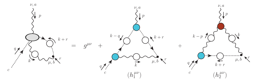
Figure 19: SDE for the ghost-gluon scattering kernel, $H_{\mu\nu}(r,q,p)$. We omit a diagram containing a 1PI four-point function.

It is well known that, in the Landau gauge, the momentum $q$ of the ghost field in $H_{\mu\nu}(r,q,p)$ factors out of its quantum corrections Marciano and Pagels (1978), allowing us to write Aguilar et al. (2019, 2020, 2022)

$$H_{\mu\nu}(r,q,p)=g_{\mu\nu}+q^{\alpha}K_{\mu\nu\alpha}(r,q,p)\,,$$ (111)

where no particular assumptions are made about the structure of the function $K_{\mu\nu\alpha}(r,q,p)$. Following Eq. (107), we differentiate the r.h.s. of Eq. (111) with respect to $q$ and subsequently set $q=0$, to obtain

$${\cal W}(r)=-\frac{1}{3}r^{\alpha}P^{\mu\nu}(r)K_{\mu\nu\alpha}(r,0,-r)\,.$$ (112)

Lastly, the finite renormalization of ${\cal W}$ proceeds through the use of Eqs. (14) and (86), which leads to the appearance of an overall factor of ${\widetilde{Z}}_{1}$ in the equations.

The outcome of the above steps is that ${\cal W}(r)$ can be written as

$${\cal W}(r)={\cal W}_{1}(r)+{\cal W}_{2}(r)\,,$$ (113)

where the ${\cal W}_{i}(r)$ are the contributions originating from the diagrams $(h_{i}^{\mu\nu})$ of Fig. 19, respectively, and read

$${\cal W}_{1}(r) = \frac{\lambda{\widetilde{Z}}_{1}}{3}\int_{k}\Delta(k)D(k)D(k+r)(r\cdot k)f(k,r)B_{1}(k+r,-k,-r)B_{1}(k,0,-k)\,,$$

$${\cal W}_{2}(r) = \frac{\lambda{\widetilde{Z}}_{1}}{3}\int_{k}\Delta(k)\Delta(k+r)D(k+r)B_{1}(k+r,0,-k-r){\cal I}_{{\cal W}}(-r,-k,k+r)\,,$$ (114)

where $f(k,r)$ is given by Eq. (80), and we define the specific contribution of the three-gluon vertex to the kernel of ${\cal W}(r^{2})$ as

$${\cal I}_{{\cal W}}(q,r,p) :=\frac{1}{2}(q-r)^{\nu}\overline{\Gamma}^{\alpha}_{\alpha\nu}(q,r,p)\,.$$ (115)

Note that, from Eq. (115) and the Bose symmetry of the $\overline{\Gamma}\vphantom{\Gamma}_{\alpha\mu\nu}(q,r,p)$ under the exchange $\{q,\alpha\}\leftrightarrow\{r,\mu\}$, it follows that

$${\cal I}_{{\cal W}}(q,r,p)={\cal I}_{{\cal W}}(r,q,p)\,.$$ (116)

At this point, by capitalizing on the planar degeneracy of $\overline{\Gamma}\vphantom{\Gamma}_{\alpha\mu\nu}(q,r,p)$ discussed in Sec. 7, we obtain a compact, and yet accurate, approximation for ${\cal I}_{{\cal W}}$. Specifically, using Eq. (77), we find

$${\cal I}_{{\cal W}}(q,r,p) \approx{\cal I}_{{\cal W}}^{0}(q,r,p)\mathit{L}_{{sg}}(s)\,,$$ (117)

where ${\cal I}_{{\cal W}}^{0}(q,r,p)$ is the tree-level value of ${\cal I}_{{\cal W}}$, given by

$${\cal I}_{{\cal W}}^{0}(q,r,p):=\frac{2f(q,r)}{p^{2}}\left[2q^{2}r^{2}-(q^{2}+r^{2})(q\cdot r)-(q\cdot r)^{2}\right]\,.$$ (118)

We remark that the approximation given by Eq. (117) becomes exact in the limit $p=0$.

Using the above approximation for ${\cal I}_{{\cal W}}$, the contribution ${\cal W}_{2}(r)$ reads

$${\cal W}_{2}(r)= \frac{2\lambda{\widetilde{Z}}_{1}}{3}\int_{k}\Delta(k)\frac{\Delta(k+r)D(k+r)}{(k+r)^{2}}B_{1}(k+r,0,-k-r)f(k,r)$$

$$\times\left[2r^{2}k^{2}-(r^{2}+k^{2})(r\cdot k)-(r\cdot k)^{2}\right]\mathit{L}_{{sg}}({\hat{s}})\,,$$ (119)

where we now have ${\hat{s}}^{2}=r^{2}+k^{2}+(r\cdot k)$.

Lastly, we transform ${\cal W}_{1}$ of Eq. (114) and ${\cal W}_{2}$ of Eq. (119) to Euclidean space to obtain the final expression to be used for the numerical determination of ${\cal W}$,

$${\cal W}_{1}(r) =-\frac{r\alpha_{s}C_{\rm A}{\widetilde{Z}}_{1}}{12\pi^{2}}\!\int_{0}^{\infty}\!dk^{2}k\Delta(k)F(k)B_{1}(k^{2},k^{2},\pi)\!\int_{0}^{\pi}\!d\phi s_{\phi}^{4}c_{\phi}\frac{F(\sqrt{z})}{z}B_{1}(z,r^{2},\chi)\,,$$

$${\cal W}_{2}(r) =-\frac{r\alpha_{s}C_{\rm A}{\widetilde{Z}}_{1}}{6\pi^{2}}\!\int_{0}^{\infty}\!dk^{2}\,k^{3}\Delta(k)\!\int_{0}^{\pi}\!d\phi\,s_{\phi}^{4}\Delta(\sqrt{z})B_{1}(z,z,\pi)\frac{F(\sqrt{z})}{z^{2}}\left[kr(2+c_{\phi}^{2})-zc_{\phi}\right]$$

$$\quad\times\mathit{L}_{{sg}}\left(r^{2}+k^{2}+rkc_{\phi}\right)\,,$$ (120)

where $z$ has been defined below Eq. (89) and

$$\chi:=\cos^{-1}\left[-\frac{(r+kc_{\phi})}{\sqrt{z}}\right]\,.$$ (121)

We emphasize that we have used into the SDEs of both $B_{1}$ and ${\cal W}$, given by Eqs. (88) and (120), respectively, the same approximation for the three-gluon vertex, namely Eq. (77). Therefore, our analyses of $B_{1}$ and ${\cal W}$ are self-consistent, in the sense that the STI in Eq. (110) is strictly preserved.

Before embarking on the numerical determination of ${\cal W}(r)$ for the entire range of Euclidean momenta, we discuss the infrared behavior of this function, and demonstrate an important self-consistency proof involving ${\mathbb{C}}(r)$.

Specifically, as discussed in Sec. 9, the $\mathit{L}_{{sg}}(r)$ and $d\Delta^{-1}(r)/dr^{2}$ that appear in Eq. (109) are infrared divergent, due to massless ghost loops present in their SDEs. Nevertheless, the BSE solutions for the amplitude ${\mathbb{C}}(r)$ are all found to be finite at $r=0$, (cf. Fig. 7)  Aguilar et al. (2012a); Binosi and Papavassiliou (2018); Aguilar et al. (2018, 2022). Therefore, in order for the WI displacement of Eq. (109) to be consistent with the finite ${\mathbb{C}}(0)$ obtained from BSE solutions, the infrared divergences of the ingredients appearing in Eq. (109) must cancel against each other.

Indeed, a careful analysis of diagram $(e_{2})$ of Fig. 16 yields

$$\lim_{r\to 0}\mathit{L}_{{sg}}(r)=\left[\frac{\alpha_{s}C_{\rm A}{\widetilde{Z}}_{1}^{3}F^{3}(0)}{96\pi}\right]\ln\left(\frac{r^{2}}{\mu^{2}}\right)\,,$$ (122)

up to infrared finite terms. Then, assuming that only $\mathit{L}_{{sg}}(r)$ and $d\Delta^{-1}/dr^{2}$ diverge and using the asymptotic form of $d\Delta(r)/dr^{2}$ given in Eq. (97) into Eq. (109), we find that the divergences do not fully cancel. Therefore, the finiteness of ${\mathbb{C}}(0)$ demands that the term ${\cal W}(r)/r^{2}$ appearing in the WI must be infrared divergent.

Now, it is evident from Eq. (120) that ${\cal W}(r)$ vanishes as $r\to 0$. Nevertheless, the ratio ${\cal W}(r)/r^{2}$ is found to diverge at the origin. Specifically, expanding Eq. (120) around $r=0$, it can be shown that ${\cal W}(r)/r^{2}$ has the asymptotic behavior

$$\lim_{r\to 0}\frac{{\cal W}(r)}{r^{2}}=-\left[\frac{\alpha_{s}C_{\rm A}{\widetilde{Z}}_{1}^{3}\Delta(0)F^{2}(0)}{96\pi}\right]\ln\left(\frac{r^{2}}{\mu^{2}}\right)\,.$$ (123)

Then, combining Eqs. (123), (122) and (123) we find that the infrared divergences in Eq. (109) cancel out exactly, leaving a finite ${\mathbb{C}}(0)$, in full agreement with the BSE results.

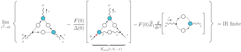
Figure 20: Diagrammatic representation of the cancellation of the infrared divergences originating from massless ghost loops in Eq. (109) to yield a finite ${\mathbb{C}}(0)$. The red cross indicates that the overall ghost momentum is factored out before being set to zero.

We finish the discussion of the infrared finiteness of ${\mathbb{C}}(0)$ with a remark. In the absence of the Schwinger mechanism, i.e., for an identically zero ${\mathbb{C}}(r)$, the infared divergences of $\mathit{L}_{{sg}}(r)$, ${\cal W}(r)/r^{2}$ and $d\Delta^{-1}(r)/dr^{2}$ must also cancel in Eq. (109). For instance, this cancellation can be explicitly verified at the one loop level, where, evidently, ${\mathbb{C}}(r)=0$. In that case, however, the gluon propagator is also massless, causing the gluonic loops contributing to the functions entering Eq. (109) to also diverge, such that the cancellation occurs among all radiative diagrams. In contrast, in the presence of a gluon mass, the cancellation of the remaining infrared divergences takes place at the level of the ghost loops only, as illustrated diagrammatically in Fig. 20.

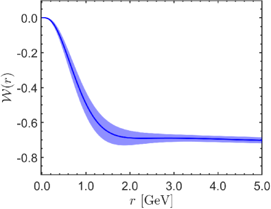
Figure 21: ${\cal W}(r)$ obtained using the approximation Eq. (117) based on the observed planar degeneracy of the three-gluon vertex in its kernel (blue solid curve) together with uncertainty estimate (blue band).

We now return to the numerical determination of ${\cal W}(r)$ from Eq. (120). To this end, we employ the fits to lattice data of Aguilar et al. (2021a) for $\Delta(q)$ and $\mathit{L}_{{sg}}(q)$ shown in Figs. 9 and 11, respectively, and the SDE solution for $F(q)$ shown in the left panel of Fig. 13. All of the fits employed are constructed so as to reproduce the correct ultraviolet behavior of the respective Green’s functions. For the value of the coupling in the asymmetric MOM scheme we employ $g^{2}=4\pi\alpha_{s}$, with $\alpha_{s}(4.3\text{ GeV})=0.27$, as determined in the lattice study of Boucaud et al. (2017). Lastly, for $B_{1}$ we use the SDE result of Sec. 8, shown in the right panel of Fig. 13, which reproduces accurately the available lattice data for the ghost-gluon vertex.

Using the above ingredients into Eq. (120) we obtain the ${\cal W}(r)$ shown as the blue solid curve in Fig. 21. The blue band in Fig. 21 represents the error estimate on our results; the procedures followed to obtain it are described in detail in Aguilar et al. (2022).

12 Displacement function from lattice inputs

In this section we determine ${\mathbb{C}}(r)$ from the main relation given in Eq. (109).

For ${\cal W}(r)$ we use the result shown in Fig. 21, together with the curves for $\mathit{L}_{{sg}}(r)$ from Fig. 11, $\Delta(r)$ and $d\Delta^{-1}(r)/dr^{2}$ from Figs. 9 and 17, respectively, and the $F(r)$ of Fig. 13. The ${\mathbb{C}}(r)$ obtained is shown as a black solid curve in the left panel of Fig. 22. In the same panel, we show as points the estimates of ${\mathbb{C}}(r)$ obtained by using into Eq. (109) the lattice data points of Ref. Aguilar et al. (2021a) directly, rather than a fit. To estimate the uncertainty in the resulting ${\mathbb{C}}(r)$, we combine the error estimate of ${\cal W}(r)$, represented by the blue band in Fig. 21, with the statistical error of the lattice data points for $\mathit{L}_{{sg}}(r)$ of Aguilar et al. (2021a), and neglect the error in the gluon propagator, which is much smaller than the errors in $\mathit{L}_{{sg}}$ and ${\cal W}$. Then, a conservative error propagation analysis produces the error bars shown in Fig. 22.

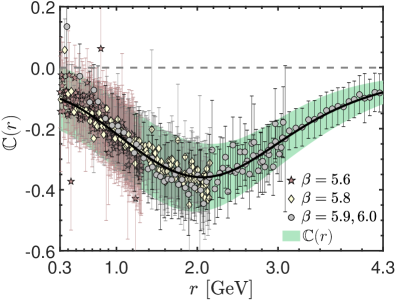
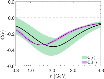
Figure 22: Left: Result for ${\mathbb{C}}(r)$ (black continuous line) obtained from Eq. (109) using the ${\cal W}(r)$ shown in Fig. 21, the fits to lattice data for $\Delta(r)$ and $\mathit{L}_{{sg}}(r)$ shown in Figs. 9 and 17, respectively, and the SDE solution for $F(r)$ shown in Fig. 13. The points are obtained using for $\mathit{L}_{{sg}}(r)$ the data in Ref. Aguilar et al. (2021a), with error bars denoting the error propagated from $\mathit{L}_{{sg}}$ and ${\cal W}$. The green band is obtained by fitting the upper and lower bounds of the points and guide the eye to the typical error associated with ${\mathbb{C}}(r)$. Right: The ${\mathbb{C}}(r)$ of the left panel is compared to the BSE prediction ${\mathbb{C}}_{\star}(r)$ (purple dot-dashed and error band) of Fig. 7.

At this point, we quantify the significance of the ${\mathbb{C}}(r)$ obtained above, in comparison to the null hypothesis result; evidently, in the absence of the Schwinger mechanism, this latter quantity, to be denoted by ${\mathbb{C}}_{0}$ in what follows, vanishes identically, namely ${\mathbb{C}}_{0}=0$. To this end, we first compute the $\chi^{2}$ of our points as

$$\chi^{2}=\sum_{i}\frac{\left[{\mathbb{C}}(r_{i})-{\mathbb{C}}_{0}(r_{i})\right]^{2}}{\epsilon_{{\scriptscriptstyle{\mathbb{C}}(r_{i})}}^{2}}\,,$$ (124)

i.e., the null hypothesis is taken as the estimator for our data. The sum runs over the $n_{r}=515$ indices $i$ such that $r_{i}\in[0.3,4.3]$ GeV, the interval of momenta for which the systematic error in our calculation of ${\cal W}(r)$ is best known, and $\epsilon_{{\scriptscriptstyle{\mathbb{C}}(r_{i})}}$ denotes the error estimate of ${\mathbb{C}}(r_{i})$. Then we obtain $\chi^{2}=2\,630$, corresponding to $\chi^{2}_{\rm d.o.f.}=5.11$. The probability $P_{{\mathbb{C}}_{0}}$ that our result for ${\mathbb{C}}$ is consistent with the null hypothesis is vanishingly small, given by the formula

$$P_{{\mathbb{C}}_{0}}=\int_{\chi^{2}=2\,630}^{\infty}\chi_{\rm{\scriptscriptstyle PDF}}^{2}(515,x)dx=\left.\frac{\Gamma(n_{r}/2,\chi^{2}/2)}{\Gamma(n_{r}/2)}\right|_{n_{r}=515}^{\chi^{2}=2\,630}=7.3\times 10^{-280}\,.$$ (125)

In fact, even if the errors were $0.95\%$ larger, i.e., nearly doubled, we could still discard ${\mathbb{C}}_{0}$ at the $5\sigma$ confidence level.

In the right panel of Fig. 22 we compare ${\mathbb{C}}(r)$ to the BSE prediction, ${\mathbb{C}}_{\star}(r)$, of Fig. 7, shown as a purple dot-dashed curve and corresponding error band. In that panel, we observe an excellent qualitative agreement between the two results. The most noticeable quantitative difference is in the position of the minimum. Specifically, ${\mathbb{C}}$ reaches the minimum value of $-0.36\pm 0.11$ at $r=1.93\begin{subarray}{c}+0.09\\ -0.06\end{subarray}$ GeV, while the minimum of ${\mathbb{C}}_{\star}$ is $-0.341\pm 0.003$ at $r=1.5\pm 0.1$.

Nevertheless, it is clear in the right panel of Fig. 22 that the BSE prediction lies within the error estimate of the lattice-derived ${\mathbb{C}}(r)$. In fact, defining a $\chi^{2}$ measure for the discrepancy between ${\mathbb{C}}$ and ${\mathbb{C}}_{\star}$ as

$$\chi^{2}_{\star}=\sum_{i}\frac{\left[{\mathbb{C}}(r_{i})-{\mathbb{C}}_{\star}(r_{i})\right]^{2}}{\epsilon_{{\scriptscriptstyle{\mathbb{C}}(r_{i})}}^{2}}\,,$$ (126)

we obtain $\chi^{2}_{\star}=258.5$, which is smaller than the number of degrees of freedom. Then, this value of $\chi^{2}_{\star}$ amounts to a probability of

$$P_{{\mathbb{C}}_{\star}}=\left.\frac{\Gamma(n_{r}/2,\chi^{2}_{\star}/2)}{\Gamma(n_{r}/2)}\right|_{n_{r}=515}^{\chi^{2}_{\star}=258.5}=1-2.0\times 10^{-23}\,,$$ (127)

showing that ${\mathbb{C}}_{\star}$ is statistically compatible with the lattice derived ${\mathbb{C}}$, with probability extremely near unit.

13 Conclusions

The gauge sector of QCD is host to a wide array of subtle mechanisms that are of vital importance for the self-consistency and infrared stability of the theory. In the present work, we have offered a comprehensive review of the intricate dynamics that account for some of the most prominent infrared phenomena, such as the generation of a gluon mass through the action of the Schwinger mechanism, the nonperturbative masslessness of the ghost, and the characteristic features induced by this particular mass pattern to the form factors of the three-gluon vertex.

The SDEs, supplemented by the judicious use of certain key results from lattice QCD, provide a robust continuum framework for carrying out such a demanding investigation. In fact, the results obtained from the SDEs are increasingly reliable, passing successfully all sorts of tests imposed on them. A particularly impressive, and certainly not isolated, case of such a success has been outlined in detail in Section 6.

Symmetry and dynamics are tightly interwoven; therefore, the information encoded in the STIs and WIs of the theory is particularly decisive for unraveling basic dynamical patterns. A striking manifestation of the profound connection between symmetry and dynamics is provided by the dual role played by the function ${\mathbb{C}}(r)$: it is both the BS amplitude of the massless states composed by a pair of gluons, and the quantity that embodies the displacement induced to the WIs by the presence of these states.

In our opinion, the determination of ${\mathbb{C}}(r)$ described in Section 12 represents a major success of the entire set of concepts and techniques surrounding the generation of a gluon mass through the action of the Schwinger mechanism. Thus, fifty years after the genesis of QCD, we seem to be closing in on the mechanism that the theory uses for curing the infrared instabilities endemic to perturbation theory. We hope to be able to report further progress in this direction in the near future.

The authors are supported by the Spanish MICINN grant PID2020-113334GB-I00. M. N. F. acknowledges financial support from Generalitat Valenciana through contract CIAPOS/2021/74. J. P. also acknowledges funding from the regional Prometeo/2019/087 from the Generalitat Valenciana.

Not applicable.

Appendix A BQIs for the BSE amplitudes

In this Appendix, we use two particular BQIs in order to relate the displacement functions ${\mathcal{C}}$ and ${\mathbb{C}}$ with their BFM counterparts ${\widetilde{\mathcal{C}}}$ and $\widetilde{\mathbb{C}}$, respectively.

The ghost-gluon vertices ${\rm{I}}\!\Gamma_{\mu}(r,p,q)$ and $\widetilde{{\rm{I}}\!\Gamma}\vphantom{{\rm{I}}\!\Gamma}_{\mu}(r,p,q)$ are related by a BQI Binosi and Papavassiliou (2009), which reads

$$\widetilde{{\rm{I}}\!\Gamma}\vphantom{{\rm{I}}\!\Gamma}_{\mu}(r,p,q) = \left\{\left[1+G(q)\right]g^{\nu}_{\mu}+L(q)\frac{q_{\mu}q^{\nu}}{q^{2}}\right\}{\rm{I}}\!\Gamma_{\nu}(r,p,q)$$ (128)

$$+F^{-1}(p)p^{\nu}K_{\mu\nu}(r,q,p)+r^{2}F^{-1}(r)K_{\mu}(r,q,p)\,,$$

where $K_{\mu}$ and $K_{\mu\nu}$ are two auxiliary functions, shown diagrammatically in Fig. 23, while $G(q)$ and $L(q)$ are the form factors of $\Lambda_{\mu\nu}(q)$, defined in Eq. (12).

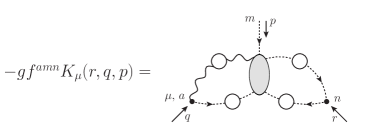
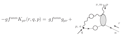
Figure 23: The auxiliary functions $K_{\mu}(q,r,p)$ and $K_{\mu\nu}(q,r,p)$, appearing in the BQI of Eq. (128).

Next, we decompose the $\widetilde{{\rm{I}}\!\Gamma}\vphantom{{\rm{I}}\!\Gamma}_{\mu}(r,p,q)$ and ${\rm{I}}\!\Gamma_{\mu}(r,p,q)$ in Eq. (128) into their regular and pole parts, using Eqs. (33) and (52), respectively. Note that the second and third terms in Eq. (128) do not contain poles in $q^{2}$; this is so because $K_{\mu\nu}(r,q,p)$ can contain (longitudinally coupled) poles only in the $p_{\nu}$ channel, whereas $K_{\mu}(r,q,p)$ has no external gluon legs, and hence no poles.

Then, multiplying Eq. (128) by $q^{2}$ we obtain

$$q_{\mu}{\widetilde{C}}(r,p,q)=q_{\mu}\left[1+G(q)+L(q)\right]C(r,p,q)+{\cal O}(q^{2})\,.$$ (129)

Setting $q=0$ in Eq. (129) and using Eq. (18), we find

$$C(r,-r,0)=Z_{1}F(0){\widetilde{C}}(r,-r,0)\,.$$ (130)

Hence, using Eq. (61), we obtain the result in Eq. (39).

Then, expanding Eq. (129) to first order in $q$, using Eq. (41) for $C(r,p,q)$ and Eq. (62) for ${\widetilde{C}}(r,p,q)$, entails

$${\mathcal{C}}(r)=Z_{1}F(0){\widetilde{\mathcal{C}}}(r)\,,$$ (131)

which is one of the main results of this Appendix.

A relation identical to Eq. (131) can be obtained for ${\mathbb{C}}(r)$ and its BFM analog, $\widetilde{\mathbb{C}}(r)$. The starting point of the derivation is the BQI Binosi and Papavassiliou (2009)

$$\widetilde{{\rm{I}}\!\Gamma}\vphantom{{\rm{I}}\!\Gamma}_{\alpha\mu\nu}(q,r,p) = \left\{\left[1+G(q)\right]g^{\rho}_{\alpha}+L(q)\frac{q_{\alpha}q^{\rho}}{q^{2}}\right\}{\rm{I}}\!\Gamma_{\rho\mu\nu}(q,r,p)$$

$$+K_{\rho\nu\alpha}(r,q,p)P^{\rho}_{\mu}(r)\Delta^{-1}(r)-K_{\rho\mu\alpha}(p,q,r)P^{\rho}_{\nu}(p)\Delta^{-1}(p)\,,$$

where $K_{\mu\nu\alpha}(r,q,p)$ is the function defined in Eq. (111).

Then, we note that the only longitudinal poles at $q=0$ present in Eq. (A) are those contained in the ${\rm{I}}\!\Gamma_{\alpha\mu\nu}(q,r,p)$ and $\widetilde{{\rm{I}}\!\Gamma}\vphantom{{\rm{I}}\!\Gamma}_{\alpha\mu\nu}(q,r,p)$ vertices, with the auxiliary functions $K_{\alpha\nu\rho}(q,p,r)$ having poles only in the $r_{\mu}$ and $p_{\nu}$ channels. As such, isolating the $q_{\alpha}g_{\mu\nu}/q^{2}$ pole and expanding around $q=0$, one eventually finds

$${\widetilde{C}}_{1}(0,r,-r)=Z_{1}^{-1}F^{-1}(0)C_{1}(0,r,-r)=0\,,$$ (133)

and

$${\mathbb{C}}(r)=Z_{1}F(0)\widetilde{\mathbb{C}}(r)\,,$$ (134)

where ${\widetilde{C}}_{1}(q,r,p)$ and $\widetilde{\mathbb{C}}(r^{2})$ are defined in analogy to the Eqs. (37) and (41), and we used Eq. (39).

References

References

- Marciano and Pagels (1978) Marciano, W.J.; Pagels, H. Quantum Chromodynamics: A Review. Phys. Rept. 1978, 36, 137. https://doi.org/10.1016/0370-1573(78)90208-9.
- Qin and Roberts (2020) Qin, S.x.; Roberts, C.D. Impressions of the Continuum Bound State Problem in QCD. Chin. Phys. Lett. 2020, 37, 121201, [arXiv:hep-ph/2008.07629]. https://doi.org/10.1088/0256-307X/37/12/121201.
- Roberts (2020) Roberts, C.D. Empirical Consequences of Emergent Mass. Symmetry 2020, 12, 1468, [arXiv:hep-ph/2009.04011]. https://doi.org/10.3390/sym12091468.
- Cui et al. (2020) Cui, Z.F.; Ding, M.; Gao, F.; Raya, K.; Binosi, D.; Chang, L.; Roberts, C.D.; Rodríguez-Quintero, J.; Schmidt, S.M. Kaon and pion parton distributions. Eur. Phys. J. C 2020, 80, 1064. https://doi.org/10.1140/epjc/s10052-020-08578-4.
- Chang and Roberts (2021) Chang, L.; Roberts, C.D. Regarding the Distribution of Glue in the Pion. Chin. Phys. Lett. 2021, 38, 081101, [arXiv:hep-ph/2106.08451]. https://doi.org/10.1088/0256-307X/38/8/081101.
- Cui et al. (2022) Cui, Z.F.; Ding, M.; Morgado, J.M.; Raya, K.; Binosi, D.; Chang, L.; De Soto, F.; Roberts, C.D.; Rodríguez-Quintero, J.; Schmidt, S.M. Emergence of pion parton distributions. Phys. Rev. D 2022, 105, L091502, [arXiv:hep-ph/2201.00884]. https://doi.org/10.1103/PhysRevD.105.L091502.
- Lu et al. (2022) Lu, Y.; Chang, L.; Raya, K.; Roberts, C.D.; Rodríguez-Quintero, J. Proton and pion distribution functions in counterpoint. Phys. Lett. B 2022, 830, 137130, [arXiv:hep-ph/2203.00753]. https://doi.org/10.1016/j.physletb.2022.137130.
- Ding et al. (2022) Ding, M.; Roberts, C.D.; Schmidt, S.M. Emergence of Hadron Mass and Structure 2022. [arXiv:hep-ph/2211.07763].
- Roberts (2022) Roberts, C.D. Origin of the Proton Mass. 2022, [arXiv:hep-ph/2211.09905].
- Roberts and Williams (1994) Roberts, C.D.; Williams, A.G. Dyson-Schwinger equations and their application to hadronic physics. Prog. Part. Nucl. Phys. 1994, 33, 477–575, [hep-ph/9403224]. https://doi.org/10.1016/0146-6410(94)90049-3.
- Alkofer and von Smekal (2001) Alkofer, R.; von Smekal, L. The Infrared behavior of QCD Green’s functions: Confinement dynamical symmetry breaking, and hadrons as relativistic bound states. Phys. Rept. 2001, 353, 281, [hep-ph/0007355]. https://doi.org/10.1016/S0370-1573(01)00010-2.
- Fischer (2006) Fischer, C.S. Infrared properties of QCD from Dyson-Schwinger equations. J. Phys. G 2006, 32, R253–R291, [hep-ph/0605173]. https://doi.org/10.1088/0954-3899/32/8/R02.
- Roberts (2008) Roberts, C.D. Hadron Properties and Dyson-Schwinger Equations. Prog. Part. Nucl. Phys. 2008, 61, 50–65, [arXiv:nucl-th/0712.0633]. https://doi.org/10.1016/j.ppnp.2007.12.034.
- Binosi and Papavassiliou (2009) Binosi, D.; Papavassiliou, J. Pinch Technique: Theory and Applications. Phys. Rept. 2009, 479, 1–152, [arXiv:hep-ph/0909.2536]. https://doi.org/10.1016/j.physrep.2009.05.001.
- Bashir et al. (2012) Bashir, A.; Chang, L.; Cloet, I.C.; El-Bennich, B.; Liu, Y.X.; et al. Collective perspective on advances in Dyson-Schwinger Equation QCD. Commun. Theor. Phys. 2012, 58, 79–134, [arXiv:nucl-th/1201.3366]. https://doi.org/10.1088/0253-6102/58/1/16.
- Binosi et al. (2015) Binosi, D.; Chang, L.; Papavassiliou, J.; Roberts, C.D. Bridging a gap between continuum-QCD and ab initio predictions of hadron observables. Phys. Lett. 2015, B742, 183–188, [arXiv:nucl-th/1412.4782]. https://doi.org/10.1016/j.physletb.2015.01.031.
- Cloet and Roberts (2014) Cloet, I.C.; Roberts, C.D. Explanation and Prediction of Observables using Continuum Strong QCD. Prog. Part. Nucl. Phys. 2014, 77, 1–69, [arXiv:nucl-th/1310.2651]. https://doi.org/10.1016/j.ppnp.2014.02.001.
- Aguilar et al. (2016) Aguilar, A.C.; Binosi, D.; Papavassiliou, J. The Gluon Mass Generation Mechanism: A Concise Primer. Front. Phys.(Beijing) 2016, 11, 111203, [arXiv:hep-ph/1511.08361]. https://doi.org/10.1007/s11467-015-0517-6.
- Binosi et al. (2016) Binosi, D.; Chang, L.; Papavassiliou, J.; Qin, S.X.; Roberts, C.D. Symmetry preserving truncations of the gap and Bethe-Salpeter equations. Phys. Rev. 2016, D93, 096010, [arXiv:nucl-th/1601.05441]. https://doi.org/10.1103/PhysRevD.93.096010.
- Binosi et al. (2017) Binosi, D.; Mezrag, C.; Papavassiliou, J.; Roberts, C.D.; Rodriguez-Quintero, J. Process-independent strong running coupling. Phys. Rev. 2017, D96, 054026, [arXiv:nucl-th/1612.04835]. https://doi.org/10.1103/PhysRevD.96.054026.
- Huber (2020) Huber, M.Q. Nonperturbative properties of Yang-Mills theories. Phys. Rept. 2020, 879, 1–92, [arXiv:hep-ph/1808.05227]. https://doi.org/10.1016/j.physrep.2020.04.004.
- Pawlowski et al. (2004) Pawlowski, J.M.; Litim, D.F.; Nedelko, S.; von Smekal, L. Infrared behavior and fixed points in Landau gauge QCD. Phys. Rev. Lett. 2004, 93, 152002, [arXiv:hep-th/hep-th/0312324]. https://doi.org/10.1103/PhysRevLett.93.152002.
- Pawlowski (2007) Pawlowski, J.M. Aspects of the functional renormalisation group. Annals Phys. 2007, 322, 2831–2915, [arXiv:hep-th/hep-th/0512261]. https://doi.org/10.1016/j.aop.2007.01.007.
- Fischer et al. (2009) Fischer, C.S.; Maas, A.; Pawlowski, J.M. On the infrared behavior of Landau gauge Yang-Mills theory. Annals Phys. 2009, 324, 2408–2437, [arXiv:hep-ph/0810.1987]. https://doi.org/10.1016/j.aop.2009.07.009.
- Carrington (2013) Carrington, M.E. Renormalization group flow equations connected to the -particle-irreducible effective action. Phys. Rev. 2013, D87, 045011, [arXiv:hep-ph/1211.4127]. https://doi.org/10.1103/PhysRevD.87.045011.
- Carrington et al. (2015) Carrington, M.E.; Fu, W.J.; Pickering, D.; Pulver, J.W. Renormalization group methods and the 2PI effective action. Phys. Rev. D 2015, 91, 025003, [arXiv:hep-ph/1404.0710]. https://doi.org/10.1103/PhysRevD.91.025003.
- Cyrol et al. (2018) Cyrol, A.K.; Mitter, M.; Pawlowski, J.M.; Strodthoff, N. Nonperturbative quark, gluon, and meson correlators of unquenched QCD. Phys. Rev. 2018, D97, 054006, [arXiv:hep-ph/1706.06326]. https://doi.org/10.1103/PhysRevD.97.054006.
- Corell et al. (2018) Corell, L.; Cyrol, A.K.; Mitter, M.; Pawlowski, J.M.; Strodthoff, N. Correlation functions of three-dimensional Yang-Mills theory from the FRG. SciPost Phys. 2018, 5, 066, [arXiv:hep-ph/1803.10092]. https://doi.org/10.21468/SciPostPhys.5.6.066.
- Huber (2020) Huber, M.Q. Correlation functions of Landau gauge Yang-Mills theory. Phys. Rev. D 2020, 101, 114009, [arXiv:hep-ph/2003.13703]. https://doi.org/10.1103/PhysRevD.101.114009.
- Dupuis et al. (2021) Dupuis, N.; Canet, L.; Eichhorn, A.; Metzner, W.; Pawlowski, J.M.; Tissier, M.; Wschebor, N. The nonperturbative functional renormalization group and its applications. Phys. Rept. 2021, 910, 1–114, [arXiv:cond-mat.stat-mech/2006.04853]. https://doi.org/10.1016/j.physrep.2021.01.001.
- Blaizot et al. (2021) Blaizot, J.P.; Pawlowski, J.M.; Reinosa, U. Functional renormalization group and 2PI effective action formalism. Annals Phys. 2021, 431, 168549, [arXiv:hep-th/2102.13628]. https://doi.org/10.1016/j.aop.2021.168549.
- Mandula and Ogilvie (1987) Mandula, J.; Ogilvie, M. The Gluon Is Massive: A Lattice Calculation of the Gluon Propagator in the Landau Gauge. Phys. Lett. B 1987, 185, 127–132. https://doi.org/10.1016/0370-2693(87)91541-3.
- Parrinello (1994) Parrinello, C. Exploratory study of the three gluon vertex on the lattice. Phys. Rev. 1994, D50, R4247–R4251, [arXiv:hep-lat/hep-lat/9405024]. https://doi.org/10.1103/PhysRevD.50.R4247.
- Alles et al. (1997) Alles, B.; Henty, D.; Panagopoulos, H.; Parrinello, C.; Pittori, C.; Richards, D.G. from the nonperturbatively renormalised lattice three gluon vertex. Nucl. Phys. 1997, B502, 325–342, [arXiv:hep-lat/hep-lat/9605033]. https://doi.org/10.1016/S0550-3213(97)00483-5.
- Parrinello et al. (1998) Parrinello, C.; Richards, D.; Alles, B.; Panagopoulos, H.; Pittori, C. Status of alpha-s determinations from the nonperturbatively renormalized three gluon vertex. Nucl. Phys. B Proc. Suppl. 1998, 63, 245–247, [hep-lat/9710053]. https://doi.org/10.1016/S0920-5632(97)00734-2.
- Boucaud et al. (1998) Boucaud, P.; Leroy, J.P.; Micheli, J.; Pene, O.; Roiesnel, C. Lattice calculation of alpha(s) in momentum scheme. J. High Energy Phys. 1998, 10, 017, [arXiv:hep-ph/hep-ph/9810322]. https://doi.org/10.1088/1126-6708/1998/10/017.
- Alexandrou et al. (2002) Alexandrou, C.; de Forcrand, P.; Follana, E. The gluon propagator without lattice Gribov copies on a finer lattice. Phys. Rev. 2002, D65, 114508, [hep-lat/0112043].
- Bowman et al. (2002) Bowman, P.O.; Heller, U.M.; Williams, A.G. Lattice quark propagator with staggered quarks in Landau and Laplacian gauges. Phys. Rev. D 2002, 66, 014505, [hep-lat/0203001]. https://doi.org/10.1103/PhysRevD.66.014505.
- Skullerud et al. (2003) Skullerud, J.I.; Bowman, P.O.; Kizilersu, A.; Leinweber, D.B.; Williams, A.G. Nonperturbative structure of the quark gluon vertex. J. High Energy Phys. 2003, 04, 047, [arXiv:hep-ph/hep-ph/0303176]. https://doi.org/10.1088/1126-6708/2003/04/047.
- Bowman et al. (2004) Bowman, P.O.; Heller, U.M.; Leinweber, D.B.; Parappilly, M.B.; Williams, A.G. Unquenched gluon propagator in Landau gauge. Phys. Rev. D 2004, 70, 034509, [hep-lat/0402032]. https://doi.org/10.1103/PhysRevD.70.034509.
- Cucchieri et al. (2006) Cucchieri, A.; Maas, A.; Mendes, T. Exploratory study of three-point Green’s functions in Landau-gauge Yang-Mills theory. Phys. Rev. 2006, D74, 014503, [arXiv:hep-lat/hep-lat/0605011]. https://doi.org/10.1103/PhysRevD.74.014503.
- Ilgenfritz et al. (2007) Ilgenfritz, E.M.; Muller-Preussker, M.; Sternbeck, A.; Schiller, A.; Bogolubsky, I. Landau gauge gluon and ghost propagators from lattice QCD. Braz.J. Phys. 2007, 37, 193–200, [arXiv:hep-lat/hep-lat/0609043]. https://doi.org/10.1590/S0103-97332007000200006.
- Sternbeck (2006) Sternbeck, A. The Infrared behavior of lattice QCD Green’s functions. PhD thesis, Humboldt-University Berlin, 2006, [arXiv:hep-lat/0609016].
- Furui and Nakajima (2006) Furui, S.; Nakajima, H. Unquenched Kogut-Susskind quark propagator in lattice Landau gauge QCD. Phys. Rev. D 2006, 73, 074503. https://doi.org/10.1103/PhysRevD.73.074503.
- Bowman et al. (2007) Bowman, P.O.; Heller, U.M.; Leinweber, D.B.; Parappilly, M.B.; Sternbeck, A.; von Smekal, L.; Williams, A.G.; Zhang, J.b. Scaling behavior and positivity violation of the gluon propagator in full QCD. Phys. Rev. D 2007, 76, 094505, [hep-lat/0703022]. https://doi.org/10.1103/PhysRevD.76.094505.
- Kamleh et al. (2007) Kamleh, W.; Bowman, P.O.; Leinweber, D.B.; Williams, A.G.; Zhang, J. Unquenching effects in the quark and gluon propagator. Phys. Rev. 2007, D76, 094501, [arXiv:hep-lat/0705.4129]. https://doi.org/10.1103/PhysRevD.76.094501.
- Cucchieri and Mendes (2007) Cucchieri, A.; Mendes, T. What’s up with IR gluon and ghost propagators in Landau gauge? A puzzling answer from huge lattices. PoS 2007, LATTICE2007, 297, [arXiv:hep-lat/0710.0412]. https://doi.org/10.22323/1.042.0297.
- Cucchieri and Mendes (2008) Cucchieri, A.; Mendes, T. Constraints on the IR behavior of the gluon propagator in Yang-Mills theories. Phys. Rev. Lett. 2008, 100, 241601, [arXiv:hep-lat/0712.3517]. https://doi.org/10.1103/PhysRevLett.100.241601.
- Bogolubsky et al. (2007) Bogolubsky, I.; Ilgenfritz, E.; Muller-Preussker, M.; Sternbeck, A. The Landau gauge gluon and ghost propagators in 4D SU(3) gluodynamics in large lattice volumes. PoS 2007, LATTICE2007, 290, [arXiv:hep-lat/0710.1968]. https://doi.org/10.22323/1.042.0290.
- Cucchieri et al. (2008) Cucchieri, A.; Maas, A.; Mendes, T. Three-point vertices in Landau-gauge Yang-Mills theory. Phys. Rev. 2008, D77, 094510, [arXiv:hep-lat/0803.1798]. https://doi.org/10.1103/PhysRevD.77.094510.
- Cucchieri and Mendes (2008) Cucchieri, A.; Mendes, T. Constraints on the IR behavior of the ghost propagator in Yang-Mills theories. Phys. Rev. D 2008, 78, 094503, [arXiv:hep-lat/0804.2371]. https://doi.org/10.1103/PhysRevD.78.094503.
- Cucchieri and Mendes (2010) Cucchieri, A.; Mendes, T. Landau-gauge propagators in Yang-Mills theories at beta = 0: Massive solution versus conformal scaling. Phys. Rev. 2010, D81, 016005, [arXiv:hep-lat/0904.4033]. https://doi.org/10.1103/PhysRevD.81.016005.
- Cucchieri and Mendes (2009) Cucchieri, A.; Mendes, T. Numerical test of the Gribov-Zwanziger scenario in Landau gauge. PoS 2009, QCD-TNT09, 026, [arXiv:hep-lat/1001.2584]. https://doi.org/10.22323/1.087.0026.
- Boucaud et al. (2009) Boucaud, P.; De Soto, F.; Leroy, J.; Le Yaouanc, A.; Micheli, J.; et al. Ghost-gluon running coupling, power corrections and the determination of Lambda(MS-bar). Phys. Rev. 2009, D79, 014508, [arXiv:hep-ph/0811.2059]. https://doi.org/10.1103/PhysRevD.79.014508.
- Cucchieri et al. (2009) Cucchieri, A.; Mendes, T.; Santos, E.M.S. Covariant gauge on the lattice: A New implementation. Phys. Rev. Lett. 2009, 103, 141602, [arXiv:hep-lat/0907.4138]. https://doi.org/10.1103/PhysRevLett.103.141602.
- Bogolubsky et al. (2009) Bogolubsky, I.; Ilgenfritz, E.; Muller-Preussker, M.; Sternbeck, A. Lattice gluodynamics computation of Landau gauge Green’s functions in the deep infrared. Phys. Lett. 2009, B676, 69–73, [arXiv:hep-lat/0901.0736]. https://doi.org/10.1016/j.physletb.2009.04.076.
- Oliveira and Silva (2009) Oliveira, O.; Silva, P. The Lattice infrared Landau gauge gluon propagator: The Infinite volume limit. PoS 2009, LAT2009, 226, [arXiv:hep-lat/0910.2897]. https://doi.org/10.22323/1.091.0226.
- Cucchieri et al. (2010) Cucchieri, A.; Mendes, T.; Nakamura, G.M.; Santos, E.M.S. Gluon Propagators in Linear Covariant Gauge. PoS 2010, FACESQCD, 026, [arXiv:hep-lat/1102.5233]. https://doi.org/10.22323/1.117.0026.
- Oliveira and Bicudo (2011) Oliveira, O.; Bicudo, P. Running Gluon Mass from Landau Gauge Lattice QCD Propagator. J. Phys. G 2011, G38, 045003, [arXiv:hep-lat/1002.4151]. https://doi.org/10.1088/0954-3899/38/4/045003.
- Blossier et al. (2010) Blossier, B.; Boucaud, P.; De soto, F.; Morenas, V.; Gravina, M.; Pene, O.; Rodriguez-Quintero, J. Ghost-gluon coupling, power corrections and from twisted-mass lattice QCD at Nf=2. Phys. Rev. D 2010, 82, 034510, [arXiv:hep-lat/1005.5290]. https://doi.org/10.1103/PhysRevD.82.034510.
- Cucchieri et al. (2010) Cucchieri, A.; Mendes, T.; Nakamura, G.M.; Santos, E.M.S. Gluon Propagators in Linear Covariant Gauge. PoS 2010, FACESQCD, 026, [arXiv:hep-lat/1102.5233]. https://doi.org/10.22323/1.117.0026.
- Maas (2013) Maas, A. Describing gauge bosons at zero and finite temperature. Phys. Rept. 2013, 524, 203–300, [arXiv:hep-ph/1106.3942]. https://doi.org/10.1016/j.physrep.2012.11.002.
- Boucaud et al. (2012) Boucaud, P.; Leroy, J.P.; Yaouanc, A.L.; Micheli, J.; Pene, O.; Rodriguez-Quintero, J. The Infrared Behaviour of the Pure Yang-Mills Green Functions. Few Body Syst. 2012, 53, 387–436, [arXiv:hep-ph/1109.1936]. https://doi.org/10.1007/s00601-011-0301-2.
- Ayala et al. (2012) Ayala, A.; Bashir, A.; Binosi, D.; Cristoforetti, M.; Rodriguez-Quintero, J. Quark flavour effects on gluon and ghost propagators. Phys. Rev. 2012, D86, 074512, [arXiv:hep-ph/1208.0795]. https://doi.org/10.1103/PhysRevD.86.074512.
- Oliveira and Silva (2012) Oliveira, O.; Silva, P.J. The lattice Landau gauge gluon propagator: lattice spacing and volume dependence. Phys. Rev. 2012, D86, 114513, [arXiv:hep-lat/1207.3029]. https://doi.org/10.1103/PhysRevD.86.114513.
- Sternbeck and Müller-Preussker (2013) Sternbeck, A.; Müller-Preussker, M. Lattice evidence for the family of decoupling solutions of Landau gauge Yang-Mills theory. Phys. Lett. B 2013, 726, 396–403, [arXiv:hep-lat/1211.3057]. https://doi.org/10.1016/j.physletb.2013.08.017.
- Bicudo et al. (2015) Bicudo, P.; Binosi, D.; Cardoso, N.; Oliveira, O.; Silva, P.J. Lattice gluon propagator in renormalizable gauges. Phys. Rev. 2015, D92, 114514, [arXiv:hep-lat/1505.05897]. https://doi.org/10.1103/PhysRevD.92.114514.
- Duarte et al. (2016) Duarte, A.G.; Oliveira, O.; Silva, P.J. Lattice Gluon and Ghost Propagators, and the Strong Coupling in Pure SU(3) Yang-Mills Theory: Finite Lattice Spacing and Volume Effects. Phys. Rev. D 2016, 94, 014502, [arXiv:hep-lat/1605.00594]. https://doi.org/10.1103/PhysRevD.94.014502.
- Athenodorou et al. (2016) Athenodorou, A.; Binosi, D.; Boucaud, P.; De Soto, F.; Papavassiliou, J.; Rodriguez-Quintero, J.; Zafeiropoulos, S. On the zero crossing of the three-gluon vertex. Phys. Lett. 2016, B761, 444–449, [arXiv:hep-ph/1607.01278]. https://doi.org/10.1016/j.physletb.2016.08.065.
- Duarte et al. (2016) Duarte, A.G.; Oliveira, O.; Silva, P.J. Further Evidence For Zero Crossing On The Three Gluon Vertex. Phys. Rev. 2016, D94, 074502, [arXiv:hep-lat/1607.03831]. https://doi.org/10.1103/PhysRevD.94.074502.
- Oliveira et al. (2016) Oliveira, O.; Kizilersu, A.; Silva, P.J.; Skullerud, J.I.; Sternbeck, A.; Williams, A.G. Lattice Landau gauge quark propagator and the quark-gluon vertex. Acta Phys. Polon. Supp. 2016, 9, 363–368, [arXiv:hep-lat/1605.09632]. https://doi.org/10.5506/APhysPolBSupp.9.363.
- Boucaud et al. (2017) Boucaud, P.; De Soto, F.; Rodríguez-Quintero, J.; Zafeiropoulos, S. Refining the detection of the zero crossing for the three-gluon vertex in symmetric and asymmetric momentum subtraction schemes. Phys. Rev. 2017, D95, 114503, [arXiv:hep-lat/1701.07390]. https://doi.org/10.1103/PhysRevD.95.114503.
- Sternbeck et al. (2017) Sternbeck, A.; Balduf, P.H.; Kizilersu, A.; Oliveira, O.; Silva, P.J.; Skullerud, J.I.; Williams, A.G. Triple-gluon and quark-gluon vertex from lattice QCD in Landau gauge. PoS 2017, LATTICE2016, 349, [arXiv:hep-lat/1702.00612]. https://doi.org/10.22323/1.256.0349.
- Boucaud et al. (2018) Boucaud, P.; De Soto, F.; Raya, K.; Rodríguez-Quintero, J.; Zafeiropoulos, S. Discretization effects on renormalized gauge-field Green’s functions, scale setting, and the gluon mass. Phys. Rev. 2018, D98, 114515, [arXiv:hep-ph/1809.05776]. https://doi.org/10.1103/PhysRevD.98.114515.
- Cucchieri et al. (2018a) Cucchieri, A.; Dudal, D.; Mendes, T.; Oliveira, O.; Roelfs, M.; Silva, P.J. Lattice Computation of the Ghost Propagator in Linear Covariant Gauges. PoS 2018, LATTICE2018, 252, [arXiv:hep-lat/1811.11521]. https://doi.org/10.22323/1.334.0252.
- Cucchieri et al. (2018b) Cucchieri, A.; Dudal, D.; Mendes, T.; Oliveira, O.; Roelfs, M.; Silva, P.J. Faddeev-Popov Matrix in Linear Covariant Gauge: First Results. Phys. Rev. D 2018, 98, 091504, [arXiv:hep-lat/1809.08224]. https://doi.org/10.1103/PhysRevD.98.091504.
- Oliveira et al. (2019) Oliveira, O.; Silva, P.J.; Skullerud, J.I.; Sternbeck, A. Quark propagator with two flavors of O(a)-improved Wilson fermions. Phys. Rev. D 2019, 99, 094506, [arXiv:hep-lat/1809.02541]. https://doi.org/10.1103/PhysRevD.99.094506.
- Dudal et al. (2018) Dudal, D.; Oliveira, O.; Silva, P.J. High precision statistical Landau gauge lattice gluon propagator computation vs. the Gribov–Zwanziger approach. Annals Phys. 2018, 397, 351–364, [arXiv:hep-lat/1803.02281]. https://doi.org/10.1016/j.aop.2018.08.019.
- Vujinovic and Mendes (2019) Vujinovic, M.; Mendes, T. Probing the tensor structure of lattice three-gluon vertex in Landau gauge. Phys. Rev. 2019, D99, 034501, [arXiv:hep-lat/1807.03673]. https://doi.org/10.1103/PhysRevD.99.034501.
- Cui et al. (2020) Cui, Z.F.; Zhang, J.L.; Binosi, D.; de Soto, F.; Mezrag, C.; Papavassiliou, J.; Roberts, C.D.; Rodríguez-Quintero, J.; Segovia, J.; Zafeiropoulos, S. Effective charge from lattice QCD. Chin. Phys. C 2020, 44, 083102, [arXiv:hep-ph/1912.08232]. https://doi.org/10.1088/1674-1137/44/8/083102.
- Zafeiropoulos et al. (2019) Zafeiropoulos, S.; Boucaud, P.; De Soto, F.; Rodríguez-Quintero, J.; Segovia, J. Strong Running Coupling from the Gauge Sector of Domain Wall Lattice QCD with Physical Quark Masses. Phys. Rev. Lett. 2019, 122, 162002, [arXiv:hep-ph/1902.08148]. https://doi.org/10.1103/PhysRevLett.122.162002.
- Aguilar et al. (2020) Aguilar, A.C.; De Soto, F.; Ferreira, M.N.; Papavassiliou, J.; Rodríguez-Quintero, J.; Zafeiropoulos, S. Gluon propagator and three-gluon vertex with dynamical quarks. Eur. Phys. J. 2020, C80, 154, [arXiv:hep-ph/1912.12086]. https://doi.org/10.1140/epjc/s10052-020-7741-0.
- Maas and Vujinović (2022) Maas, A.; Vujinović, M. More on the three-gluon vertex in SU(2) Yang-Mills theory in three and four dimensions. SciPost Phys. Core 2022, 5, 019, [arXiv:hep-lat/2006.08248]. https://doi.org/10.21468/SciPostPhysCore.5.2.019.
- Kızılersü et al. (2021) Kızılersü, A.; Oliveira, O.; Silva, P.J.; Skullerud, J.I.; Sternbeck, A. Quark-gluon vertex from Nf=2 lattice QCD. Phys. Rev. D 2021, 103, 114515, [arXiv:hep-lat/2103.02945]. https://doi.org/10.1103/PhysRevD.103.114515.
- Aguilar et al. (2021a) Aguilar, A.C.; De Soto, F.; Ferreira, M.N.; Papavassiliou, J.; Rodríguez-Quintero, J. Infrared facets of the three-gluon vertex. Phys. Lett. B 2021, 818, 136352, [arXiv:hep-ph/2102.04959]. https://doi.org/10.1016/j.physletb.2021.136352.
- Aguilar et al. (2021b) Aguilar, A.C.; Ambrósio, C.O.; De Soto, F.; Ferreira, M.N.; Oliveira, B.M.; Papavassiliou, J.; Rodríguez-Quintero, J. Ghost dynamics in the soft gluon limit. Phys. Rev. D 2021, 104, 054028, [arXiv:hep-ph/2107.00768]. https://doi.org/10.1103/PhysRevD.104.054028.
- Pinto-Gómez et al. (2022) Pinto-Gómez, F.; De Soto, F.; Ferreira, M.N.; Papavassiliou, J.; Rodríguez-Quintero, J. Lattice three-gluon vertex in extended kinematics: planar degeneracy 2022. [arXiv:hep-ph/2208.01020].
- Pinto-Gomez and de Soto (2022) Pinto-Gomez, F.; de Soto, F. Three-gluon vertex in Landau-gauge from quenched-lattice QCD in general kinematics. In Proceedings of the 15th Conference on Quark Confinement and the Hadron Spectrum, 2022, [arXiv:hep-lat/2211.12199].
- Pinto-Gómez et al. (2022) Pinto-Gómez, F.; de Soto, F.; Ferreira, M.N.; Papavassiliou, J.; Rodríguez-Quintero, J. General kinematics of the three-gluon vertex from quenched lattice QCD. 2022, [arXiv:hep-lat/2212.11894].
- Roberts and Schmidt (2020) Roberts, C.D.; Schmidt, S.M. Reflections upon the emergence of hadronic mass. Eur. Phys. J. ST 2020, 229, 3319–3340, [arXiv:hep-ph/2006.08782]. https://doi.org/10.1140/epjst/e2020-000064-6.
- Roberts (2021) Roberts, C.D. On Mass and Matter. AAPPS Bull. 2021, 31, 6, [arXiv:hep-ph/2101.08340]. https://doi.org/10.1007/s43673-021-00005-4.
- Roberts et al. (2021) Roberts, C.D.; Richards, D.G.; Horn, T.; Chang, L. Insights into the emergence of mass from studies of pion and kaon structure. Prog. Part. Nucl. Phys. 2021, 120, 103883, [arXiv:hep-ph/2102.01765]. https://doi.org/10.1016/j.ppnp.2021.103883.
- Binosi (2022) Binosi, D. Emergent Hadron Mass in Strong Dynamics. Few Body Syst. 2022, 63, 42, [arXiv:hep-ph/2203.00942]. https://doi.org/10.1007/s00601-022-01740-6.
- Papavassiliou (2022) Papavassiliou, J. Emergence of mass in the gauge sector of QCD*. Chin. Phys. C 2022, 46, 112001, [arXiv:hep-ph/2207.04977]. https://doi.org/10.1088/1674-1137/ac84ca.
- Cornwall (1979) Cornwall, J.M. Quark Confinement and Vortices in Massive Gauge Invariant QCD. Nucl. Phys. 1979, B157, 392.
- Parisi and Petronzio (1980) Parisi, G.; Petronzio, R. On Low-Energy Tests of QCD. Phys. Lett. 1980, B94, 51.
- Cornwall (1982) Cornwall, J.M. Dynamical Mass Generation in Continuum QCD. Phys. Rev. D 1982, 26, 1453. https://doi.org/10.1103/PhysRevD.26.1453.
- Bernard (1982) Bernard, C.W. Monte Carlo Evaluation of the Effective Gluon Mass. Phys. Lett. B 1982, 108, 431–434. https://doi.org/10.1016/0370-2693(82)91228-X.
- Bernard (1983) Bernard, C.W. Adjoint Wilson Lines and the Effective Gluon Mass. Nucl. Phys. B 1983, 219, 341–357. https://doi.org/10.1016/0550-3213(83)90645-4.
- Donoghue (1984) Donoghue, J.F. The Gluon ’Mass’ in the Bag Model. Phys. Rev. D 1984, 29, 2559. https://doi.org/10.1103/PhysRevD.29.2559.
- Cornwall and Papavassiliou (1989) Cornwall, J.M.; Papavassiliou, J. Gauge Invariant Three Gluon Vertex in QCD. Phys. Rev. D 1989, 40, 3474. https://doi.org/10.1103/PhysRevD.40.3474.
- Lavelle (1991) Lavelle, M. Gauge invariant effective gluon mass from the operator product expansion. Phys. Rev. D 1991, 44, 26–28. https://doi.org/10.1103/PhysRevD.44.R26.
- Halzen et al. (1993) Halzen, F.; Krein, G.I.; Natale, A.A. Relating the QCD pomeron to an effective gluon mass. Phys. Rev. 1993, D47, 295–298.
- Wilson et al. (1994) Wilson, K.G.; Walhout, T.S.; Harindranath, A.; Zhang, W.M.; Perry, R.J.; Glazek, S.D. Nonperturbative QCD: A Weak coupling treatment on the light front. Phys. Rev. 1994, D49, 6720–6766, [arXiv:hep-th/hep-th/9401153]. https://doi.org/10.1103/PhysRevD.49.6720.
- Mihara and Natale (2000) Mihara, A.; Natale, A.A. Dynamical gluon mass corrections in heavy quarkonia decays. Phys. Lett. 2000, B482, 378–382, [hep-ph/0004236].
- Philipsen (2002) Philipsen, O. On the nonperturbative gluon mass and heavy quark physics. Nucl. Phys. 2002, B628, 167–192, [arXiv:hep-lat/hep-lat/0112047]. https://doi.org/10.1016/S0550-3213(02)00089-5.
- Kondo (2001) Kondo, K.I. Vacuum condensate of mass dimension 2 as the origin of mass gap and quark confinement. Phys. Lett. 2001, B514, 335–345, [hep-th/0105299].
- Aguilar et al. (2003) Aguilar, A.C.; Natale, A.A.; Rodrigues da Silva, P.S. Relating a gluon mass scale to an infrared fixed point in pure gauge QCD. Phys. Rev. Lett. 2003, 90, 152001, [hep-ph/0212105]. https://doi.org/10.1103/PhysRevLett.90.152001.
- Aguilar and Natale (2004) Aguilar, A.C.; Natale, A.A. A Dynamical gluon mass solution in a coupled system of the Schwinger-Dyson equations. J. High Energy Phys. 2004, 08, 057, [hep-ph/0408254]. https://doi.org/10.1088/1126-6708/2004/08/057.
- Aguilar and Papavassiliou (2006) Aguilar, A.C.; Papavassiliou, J. Gluon mass generation in the PT-BFM scheme. J. High Energy Phys. 2006, 12, 012, [hep-ph/0610040]. https://doi.org/10.1088/1126-6708/2006/12/012.
- Epple et al. (2008) Epple, D.; Reinhardt, H.; Schleifenbaum, W.; Szczepaniak, A.P. Subcritical solution of the Yang-Mills Schroedinger equation in the Coulomb gauge. Phys. Rev. 2008, D77, 085007, [arXiv:hep-th/0712.3694]. https://doi.org/10.1103/PhysRevD.77.085007.
- Aguilar and Papavassiliou (2007) Aguilar, A.C.; Papavassiliou, J. On dynamical gluon mass generation. Eur.Phys.J. 2007, A31, 742–745, [arXiv:hep-ph/0704.2308]. https://doi.org/10.1140/epja/i2006-10281-7.
- Aguilar et al. (2008) Aguilar, A.C.; Binosi, D.; Papavassiliou, J. Gluon and ghost propagators in the Landau gauge: Deriving lattice results from Schwinger-Dyson equations. Phys. Rev. 2008, D78, 025010, [arXiv:hep-ph/0802.1870]. https://doi.org/10.1103/PhysRevD.78.025010.
- Aguilar and Papavassiliou (2010) Aguilar, A.C.; Papavassiliou, J. Gluon mass generation without seagull divergences. Phys. Rev. 2010, D81, 034003, [arXiv:hep-ph/0910.4142]. https://doi.org/10.1103/PhysRevD.81.034003.
- Campagnari and Reinhardt (2010) Campagnari, D.R.; Reinhardt, H. Non-Gaussian wave functionals in Coulomb gauge Yang–Mills theory. Phys. Rev. 2010, D82, 105021, [arXiv:hep-th/1009.4599]. https://doi.org/10.1103/PhysRevD.82.105021.
- Fagundes et al. (2012) Fagundes, D.A.; Luna, E.G.S.; Menon, M.J.; Natale, A.A. Aspects of a Dynamical Gluon Mass Approach to Elastic Hadron Scattering at LHC. Nucl. Phys. A 2012, 886, 48–70, [arXiv:hep-ph/1112.4680]. https://doi.org/10.1016/j.nuclphysa.2012.05.002.
- Aguilar et al. (2011) Aguilar, A.C.; Binosi, D.; Papavassiliou, J. The dynamical equation of the effective gluon mass. Phys. Rev. 2011, D84, 085026, [arXiv:hep-ph/1107.3968]. https://doi.org/10.1103/PhysRevD.84.085026.
- Aguilar et al. (2012a) Aguilar, A.C.; Ibanez, D.; Mathieu, V.; Papavassiliou, J. Massless bound-state excitations and the Schwinger mechanism in QCD. Phys. Rev. 2012, D85, 014018, [arXiv:hep-ph/1110.2633]. https://doi.org/10.1103/PhysRevD.85.014018.
- Aguilar et al. (2012b) Aguilar, A.C.; Binosi, D.; Papavassiliou, J. Gluon mass through ghost synergy. J. High Energy Phys. 2012, 01, 050, [arXiv:hep-ph/1108.5989]. https://doi.org/10.1007/JHEP01(2012)050.
- Aguilar et al. (2013) Aguilar, A.C.; Binosi, D.; Papavassiliou, J. Gluon mass generation in the presence of dynamical quarks. Phys. Rev. 2013, D88, 074010, [arXiv:hep-ph/1304.5936]. https://doi.org/10.1103/PhysRevD.88.074010.
- Glazek et al. (2017) Glazek, S.D.; Gómez-Rocha, M.; More, J.; Serafin, K. Renormalized quark–antiquark Hamiltonian induced by a gluon mass ansatz in heavy-flavor QCD. Phys. Lett. 2017, B773, 172–178, [arXiv:hep-ph/1705.07629]. https://doi.org/10.1016/j.physletb.2017.08.018.
- Binosi and Papavassiliou (2018) Binosi, D.; Papavassiliou, J. Coupled dynamics in gluon mass generation and the impact of the three-gluon vertex. Phys. Rev. 2018, D97, 054029, [arXiv:hep-ph/1709.09964]. https://doi.org/10.1103/PhysRevD.97.054029.
- Aguilar et al. (2019) Aguilar, A.C.; Ferreira, M.N.; Figueiredo, C.T.; Papavassiliou, J. Gluon mass scale through nonlinearities and vertex interplay. Phys. Rev. D 2019, 100, 094039, [arXiv:hep-ph/1909.09826]. https://doi.org/10.1103/PhysRevD.100.094039.
- Eichmann et al. (2021) Eichmann, G.; Pawlowski, J.M.; Silva, J.M. Mass generation in Landau-gauge Yang-Mills theory. Phys. Rev. D 2021, 104, 114016, [arXiv:hep-ph/2107.05352]. https://doi.org/10.1103/PhysRevD.104.114016.
- Aguilar et al. (2022) Aguilar, A.C.; Ferreira, M.N.; Papavassiliou, J. Exploring smoking-gun signals of the Schwinger mechanism in QCD. Phys. Rev. D 2022, 105, 014030, [arXiv:hep-ph/2111.09431]. https://doi.org/10.1103/PhysRevD.105.014030.
- Horak et al. (2022) Horak, J.; Ihssen, F.; Papavassiliou, J.; Pawlowski, J.M.; Weber, A.; Wetterich, C. Gluon condensates and effective gluon mass. SciPost Phys. 2022, 13, 042, [arXiv:hep-ph/2201.09747]. https://doi.org/10.21468/SciPostPhys.13.2.042.
- Aguilar et al. (2022) Aguilar, A.C.; De Soto, F.; Ferreira, M.N.; Papavassiliou, J.; Pinto-Gómez, F.; Roberts, C.D.; Rodríguez-Quintero, J. Schwinger mechanism for gluons from lattice QCD 2022. [arXiv:hep-ph/2211.12594].
- Schwinger (1962a) Schwinger, J.S. Gauge Invariance and Mass. Phys. Rev. 1962, 125, 397–398. https://doi.org/10.1103/PhysRev.125.397.
- Schwinger (1962b) Schwinger, J.S. Gauge Invariance and Mass. 2. Phys. Rev. 1962, 128, 2425–2429. https://doi.org/10.1103/PhysRev.128.2425.
- Watson (1997) Watson, N.J. The gauge-independent QCD effective charge. Nucl. Phys. 1997, B494, 388–432, [hep-ph/9606381].
- Binosi and Papavassiliou (2003) Binosi, D.; Papavassiliou, J. The QCD effective charge to all orders. Nucl. Phys. Proc. Suppl. 2003, 121, 281–284, [arXiv:hep-ph/hep-ph/0209016]. https://doi.org/10.1016/S0920-5632(03)01862-0.
- Aguilar et al. (2009) Aguilar, A.C.; Binosi, D.; Papavassiliou, J.; Rodriguez-Quintero, J. Non-perturbative comparison of QCD effective charges. Phys. Rev. 2009, D80, 085018, [arXiv:hep-ph/0906.2633]. https://doi.org/10.1103/PhysRevD.80.085018.
- Gell-Mann and Low (1954) Gell-Mann, M.; Low, F.E. Quantum electrodynamics at small distances. Phys. Rev. 1954, 95, 1300–1312. https://doi.org/10.1103/PhysRev.95.1300.
- Itzykson and Zuber (1980) Itzykson, C.; Zuber, J.B. Quantum Field Theory; International Series in Pure and Applied Physics, New York, USA: Mcgraw-Hill (1980) 705 p., 1980.
- Nambu and Jona-Lasinio (1961) Nambu, Y.; Jona-Lasinio, G. Dynamical model of elementary particles based on an analogy with superconductivity. I. Phys. Rev. 1961, 122, 345–358. https://doi.org/10.1103/PhysRev.122.345.
- Lane (1974) Lane, K.D. Asymptotic Freedom and Goldstone Realization of Chiral Symmetry. Phys. Rev. 1974, D10, 2605.
- Politzer (1976) Politzer, H.D. Effective Quark Masses in the Chiral Limit. Nucl. Phys. 1976, B117, 397.
- Miransky and Fomin (1981) Miransky, V.A.; Fomin, P.I. CHIRAL SYMMETRY BREAKDOWN AND THE SPECTRUM OF PSEUDOSCALAR MESONS IN QUANTUM CHROMODYNAMICS. Phys. Lett. 1981, B105, 387–391.
- Atkinson and Johnson (1988) Atkinson, D.; Johnson, P.W. Chiral Symmetry Breaking in QCD. 2. Running Coupling Constant. Phys. Rev. 1988, D37, 2296–2299. https://doi.org/10.1103/PhysRevD.37.2296.
- Brown and Pennington (1988) Brown, N.; Pennington, M.R. STUDIES OF CONFINEMENT: HOW QUARKS AND GLUONS PROPAGATE. Phys. Rev. 1988, D38, 2266.
- Williams et al. (1991) Williams, A.G.; Krein, G.; Roberts, C.D. QUARK PROPAGATOR IN AN ANSATZ APPROACH TO QCD. Annals Phys. 1991, 210, 464–485.
- Papavassiliou and Cornwall (1991) Papavassiliou, J.; Cornwall, J.M. Coupled fermion gap and vertex equations for chiral symmetry breakdown in QCD. Phys. Rev. 1991, D44, 1285–1297.
- Hawes et al. (1994) Hawes, F.T.; Roberts, C.D.; Williams, A.G. Dynamical chiral symmetry breaking and confinement with an infrared vanishing gluon propagator. Phys. Rev. 1994, D49, 4683–4693, [arXiv:hep-ph/hep-ph/9309263]. https://doi.org/10.1103/PhysRevD.49.4683.
- Natale and Rodrigues da Silva (1997) Natale, A.A.; Rodrigues da Silva, P.S. Critical coupling for dynamical chiral-symmetry breaking with an infrared finite gluon propagator. Phys. Lett. 1997, B392, 444–451, [hep-ph/9611441].
- Fischer and Alkofer (2003) Fischer, C.S.; Alkofer, R. Nonperturbative propagators, running coupling and dynamical quark mass of Landau gauge QCD. Phys. Rev. 2003, D67, 094020, [arXiv:hep-ph/hep-ph/0301094]. https://doi.org/10.1103/PhysRevD.67.094020.
- Maris and Roberts (2003) Maris, P.; Roberts, C.D. Dyson-Schwinger equations: A Tool for hadron physics. Int. J. Mod. Phys. 2003, E12, 297–365, [arXiv:nucl-th/nucl-th/0301049]. https://doi.org/10.1142/S0218301303001326.
- Aguilar et al. (2005) Aguilar, A.C.; Nesterenko, A.; Papavassiliou, J. Infrared enhanced analytic coupling and chiral symmetry breaking in QCD. J. Phys. 2005, G31, 997, [arXiv:hep-ph/hep-ph/0504195]. https://doi.org/10.1088/0954-3899/31/9/002.
- Bowman et al. (2005) Bowman, P.O.; Heller, U.M.; Leinweber, D.B.; Parappilly, M.B.; Williams, A.G.; Zhang, J.b. Unquenched quark propagator in Landau gauge. Phys. Rev. 2005, D71, 054507, [arXiv:hep-lat/hep-lat/0501019]. https://doi.org/10.1103/PhysRevD.71.054507.
- Sauli et al. (2007) Sauli, V.; Adam, Jr., J.; Bicudo, P. Dynamical chiral symmetry breaking with integral Minkowski representations. Phys. Rev. 2007, D75, 087701, [arXiv:hep-ph/hep-ph/0607196]. https://doi.org/10.1103/PhysRevD.75.087701.
- Cornwall (2008) Cornwall, J.M. Center vortices, the functional Schrodinger equation, and CSB. In Proceedings of the 419th WE-Heraeus-Seminar: Approaches to Quantum Chromodynamics, 2008, [arXiv:hep-ph/0812.0359].
- Alkofer et al. (2009) Alkofer, R.; Fischer, C.S.; Llanes-Estrada, F.J.; Schwenzer, K. The Quark-gluon vertex in Landau gauge QCD: Its role in dynamical chiral symmetry breaking and quark confinement. Annals Phys. 2009, 324, 106–172, [arXiv:hep-ph/0804.3042]. https://doi.org/10.1016/j.aop.2008.07.001.
- Aguilar and Papavassiliou (2011) Aguilar, A.C.; Papavassiliou, J. Chiral symmetry breaking with lattice propagators. Phys. Rev. 2011, D83, 014013, [arXiv:hep-ph/1010.5815]. https://doi.org/10.1103/PhysRevD.83.014013.
- Rojas et al. (2013) Rojas, E.; de Melo, J.; El-Bennich, B.; Oliveira, O.; Frederico, T. On the Quark-Gluon Vertex and Quark-Ghost Kernel: combining Lattice Simulations with Dyson-Schwinger equations. J. High Energy Phys. 2013, 10, 193, [arXiv:hep-ph/1306.3022]. https://doi.org/10.1007/JHEP10(2013)193.
- Mitter et al. (2015) Mitter, M.; Pawlowski, J.M.; Strodthoff, N. Chiral symmetry breaking in continuum QCD. Phys. Rev. 2015, D91, 054035, [arXiv:hep-ph/1411.7978]. https://doi.org/10.1103/PhysRevD.91.054035.
- Braun et al. (2016) Braun, J.; Fister, L.; Pawlowski, J.M.; Rennecke, F. From Quarks and Gluons to Hadrons: Chiral Symmetry Breaking in Dynamical QCD. Phys. Rev. 2016, D94, 034016, [arXiv:hep-ph/1412.1045]. https://doi.org/10.1103/PhysRevD.94.034016.
- Heupel et al. (2014) Heupel, W.; Goecke, T.; Fischer, C.S. Beyond Rainbow-Ladder in bound state equations. Eur. Phys. J. 2014, A50, 85, [arXiv:hep-ph/1402.5042]. https://doi.org/10.1140/epja/i2014-14085-x.
- Binosi et al. (2017) Binosi, D.; Chang, L.; Papavassiliou, J.; Qin, S.X.; Roberts, C.D. Natural constraints on the gluon-quark vertex. Phys. Rev. 2017, D95, 031501, [arXiv:nucl-th/1609.02568]. https://doi.org/10.1103/PhysRevD.95.031501.
- Aguilar et al. (2018) Aguilar, A.C.; Cardona, J.C.; Ferreira, M.N.; Papavassiliou, J. Quark gap equation with non-abelian Ball-Chiu vertex. Phys. Rev. 2018, D98, 014002, [arXiv:hep-ph/1804.04229]. https://doi.org/10.1103/PhysRevD.98.014002.
- Gao et al. (2021) Gao, F.; Papavassiliou, J.; Pawlowski, J.M. Fully coupled functional equations for the quark sector of QCD. Phys. Rev. D 2021, 103, 094013, [arXiv:hep-ph/2102.13053]. https://doi.org/10.1103/PhysRevD.103.094013.
- Eichten and Feinberg (1974) Eichten, E.; Feinberg, F. Dynamical Symmetry Breaking of Nonabelian Gauge Symmetries. Phys. Rev. D 1974, 10, 3254–3279. https://doi.org/10.1103/PhysRevD.10.3254.
- Smit (1974) Smit, J. On the Possibility That Massless Yang-Mills Fields Generate Massive Vector Particles. Phys. Rev. D 1974, 10, 2473. https://doi.org/10.1103/PhysRevD.10.2473.
- Binosi et al. (2012) Binosi, D.; Ibañez, D.; Papavassiliou, J. The all-order equation of the effective gluon mass. Phys. Rev. 2012, D86, 085033, [arXiv:hep-ph/1208.1451]. https://doi.org/10.1103/PhysRevD.86.085033.
- Tissier and Wschebor (2010) Tissier, M.; Wschebor, N. Infrared propagators of Yang-Mills theory from perturbation theory. Phys. Rev. D 2010, 82, 101701, [arXiv:hep-ph/1004.1607]. https://doi.org/10.1103/PhysRevD.82.101701.
- Serreau and Tissier (2012) Serreau, J.; Tissier, M. Lifting the Gribov ambiguity in Yang-Mills theories. Phys. Lett. 2012, B712, 97–103, [arXiv:hep-th/1202.3432]. https://doi.org/10.1016/j.physletb.2012.04.041.
- Peláez et al. (2014) Peláez, M.; Tissier, M.; Wschebor, N. Two-point correlation functions of QCD in the Landau gauge. Phys. Rev. D 2014, 90, 065031, [arXiv:hep-th/1407.2005]. https://doi.org/10.1103/PhysRevD.90.065031.
- Siringo (2016) Siringo, F. Analytical study of Yang–Mills theory in the infrared from first principles. Nucl. Phys. 2016, B907, 572–596, [arXiv:hep-ph/1511.01015]. https://doi.org/10.1016/j.nuclphysb.2016.04.028.
- Aguilar et al. (2016) Aguilar, A.C.; Binosi, D.; Figueiredo, C.T.; Papavassiliou, J. Unified description of seagull cancellations and infrared finiteness of gluon propagators. Phys. Rev. 2016, D94, 045002, [arXiv:hep-ph/1604.08456]. https://doi.org/10.1103/PhysRevD.94.045002.
- Osterwalder and Schrader (1973) Osterwalder, K.; Schrader, R. AXIOMS FOR EUCLIDEAN GREEN’S FUNCTIONS. Commun. Math. Phys. 1973, 31, 83–112. https://doi.org/10.1007/BF01645738.
- Osterwalder and Schrader (1975) Osterwalder, K.; Schrader, R. Axioms for Euclidean Green’s Functions. 2. Commun. Math. Phys. 1975, 42, 281. https://doi.org/10.1007/BF01608978.
- Glimm and Jaffe (1981) Glimm, J.; Jaffe, A.M. QUANTUM PHYSICS. A FUNCTIONAL INTEGRAL POINT OF VIEW; 1981.
- Krein et al. (1992) Krein, G.; Roberts, C.D.; Williams, A.G. On the implications of confinement. Int. J. Mod. Phys. 1992, A7, 5607–5624. https://doi.org/10.1142/S0217751X92002544.
- Cornwall (2013) Cornwall, J.M. Positivity violations in QCD. Mod. Phys. Lett. 2013, A28, 1330035, [arXiv:hep-ph/1310.7897]. https://doi.org/10.1142/S0217732313300358.
- Aguilar et al. (2014) Aguilar, A.C.; Binosi, D.; Ibañez, D.; Papavassiliou, J. Effects of divergent ghost loops on the Green’s functions of QCD. Phys. Rev. 2014, D89, 085008, [arXiv:hep-ph/1312.1212]. https://doi.org/10.1103/PhysRevD.89.085008.
- Pelaez et al. (2013) Pelaez, M.; Tissier, M.; Wschebor, N. Three-point correlation functions in Yang-Mills theory. Phys. Rev. 2013, D88, 125003, [arXiv:hep-th/1310.2594]. https://doi.org/10.1103/PhysRevD.88.125003.
- Blum et al. (2014) Blum, A.; Huber, M.Q.; Mitter, M.; von Smekal, L. Gluonic three-point correlations in pure Landau gauge QCD. Phys. Rev. 2014, D89, 061703, [arXiv:hep-ph/1401.0713]. https://doi.org/10.1103/PhysRevD.89.061703.
- Eichmann et al. (2014) Eichmann, G.; Williams, R.; Alkofer, R.; Vujinovic, M. The three-gluon vertex in Landau gauge. Phys. Rev. 2014, D89, 105014, [arXiv:hep-ph/1402.1365]. https://doi.org/10.1103/PhysRevD.89.105014.
- Williams et al. (2016) Williams, R.; Fischer, C.S.; Heupel, W. Light mesons in QCD and unquenching effects from the 3PI effective action. Phys. Rev. 2016, D93, 034026, [arXiv:hep-ph/1512.00455]. https://doi.org/10.1103/PhysRevD.93.034026.
- Blum et al. (2015) Blum, A.L.; Alkofer, R.; Huber, M.Q.; Windisch, A. Unquenching the three-gluon vertex: A status report. Acta Phys. Polon. Supp. 2015, 8, 321, [arXiv:hep-ph/1506.04275]. https://doi.org/10.5506/APhysPolBSupp.8.321.
- Cyrol et al. (2016) Cyrol, A.K.; Fister, L.; Mitter, M.; Pawlowski, J.M.; Strodthoff, N. Landau gauge Yang-Mills correlation functions. Phys. Rev. 2016, D94, 054005, [arXiv:hep-ph/1605.01856]. https://doi.org/10.1103/PhysRevD.94.054005.
- Aguilar et al. (2019) Aguilar, A.C.; Ferreira, M.N.; Figueiredo, C.T.; Papavassiliou, J. Nonperturbative Ball-Chiu construction of the three-gluon vertex. Phys. Rev. 2019, D99, 094010, [arXiv:hep-ph/1903.01184]. https://doi.org/10.1103/PhysRevD.99.094010.
- Barrios et al. (2022) Barrios, N.; Peláez, M.; Reinosa, U. Two-loop three-gluon vertex from the Curci-Ferrari model and its leading infrared behavior to all loop orders. Phys. Rev. D 2022, 106, 114039, [arXiv:hep-ph/2207.10704]. https://doi.org/10.1103/PhysRevD.106.114039.
- Rivers (1988) Rivers, R.J. Path integral methods in quantum field theory; Cambridge Monographs on Mathematical Physics, Cambridge University Press, 1988. https://doi.org/10.1017/CBO9780511564055.
- Fujikawa et al. (1972) Fujikawa, K.; Lee, B.W.; Sanda, A.I. Generalized Renormalizable Gauge Formulation of Spontaneously Broken Gauge Theories. Phys. Rev. D 1972, 6, 2923–2943. https://doi.org/10.1103/PhysRevD.6.2923.
- Aguilar and Papavassiliou (2008) Aguilar, A.C.; Papavassiliou, J. Infrared finite ghost propagator in the Feynman gauge. Phys. Rev. 2008, D77, 125022, [arXiv:hep-ph/0712.0780]. https://doi.org/10.1103/PhysRevD.77.125022.
- Huber et al. (2010) Huber, M.Q.; Schwenzer, K.; Alkofer, R. On the infrared scaling solution of SU(N) Yang-Mills theories in the maximally Abelian gauge. Eur. Phys. J. C 2010, 68, 581–600, [arXiv:hep-th/0904.1873]. https://doi.org/10.1140/epjc/s10052-010-1371-x.
- Siringo (2014) Siringo, F. Gluon propagator in Feynman gauge by the method of stationary variance. Phys. Rev. D 2014, 90, 094021, [arXiv:hep-ph/1408.5313]. https://doi.org/10.1103/PhysRevD.90.094021.
- Aguilar et al. (2015) Aguilar, A.C.; Binosi, D.; Papavassiliou, J. Yang-Mills two-point functions in linear covariant gauges. Phys. Rev. 2015, D91, 085014, [arXiv:hep-ph/1501.07150]. https://doi.org/10.1103/PhysRevD.91.085014.
- Huber (2015) Huber, M.Q. Gluon and ghost propagators in linear covariant gauges. Phys. Rev. 2015, D91, 085018, [arXiv:hep-ph/1502.04057]. https://doi.org/10.1103/PhysRevD.91.085018.
- Capri et al. (2015) Capri, M.A.L.; Fiorentini, D.; Guimaraes, M.S.; Mintz, B.W.; Palhares, L.F.; Sorella, S.P.; Dudal, D.; Justo, I.F.; Pereira, A.D.; Sobreiro, R.F. Exact nilpotent nonperturbative BRST symmetry for the Gribov-Zwanziger action in the linear covariant gauge. Phys. Rev. D 2015, 92, 045039. https://doi.org/10.1103/PhysRevD.92.045039.
- Aguilar et al. (2017) Aguilar, A.C.; Binosi, D.; Papavassiliou, J. Schwinger mechanism in linear covariant gauges. Phys. Rev. 2017, D95, 034017, [arXiv:hep-ph/1611.02096]. https://doi.org/10.1103/PhysRevD.95.034017.
- De Meerleer et al. (2020) De Meerleer, T.; Dudal, D.; Sorella, S.P.; Dall’Olio, P.; Bashir, A. Landau-Khalatnikov-Fradkin Transformations, Nielsen Identities, Their Equivalence and Implications for QCD. Phys. Rev. D 2020, 101, 085005, [arXiv:hep-th/1911.01907]. https://doi.org/10.1103/PhysRevD.101.085005.
- Napetschnig et al. (2021) Napetschnig, M.; Alkofer, R.; Huber, M.Q.; Pawlowski, J.M. Yang-Mills propagators in linear covariant gauges from Nielsen identities. Phys. Rev. D 2021, 104, 054003, [arXiv:hep-ph/2106.12559]. https://doi.org/10.1103/PhysRevD.104.054003.
- Binosi and Papavassiliou (2008) Binosi, D.; Papavassiliou, J. Gauge-invariant truncation scheme for the Schwinger-Dyson equations of QCD. Phys. Rev. 2008, D77, 061702, [arXiv:hep-ph/0712.2707]. https://doi.org/10.1103/PhysRevD.77.061702.
- Pilaftsis (1997) Pilaftsis, A. Generalized pinch technique and the background field method in general gauges. Nucl. Phys. B 1997, 487, 467–491, [hep-ph/9607451]. https://doi.org/10.1016/S0550-3213(96)00686-4.
- Binosi and Papavassiliou (2002) Binosi, D.; Papavassiliou, J. The Pinch technique to all orders. Phys. Rev. D 2002, 66, 111901, [hep-ph/0208189]. https://doi.org/10.1103/PhysRevD.66.111901.
- Binosi and Papavassiliou (2004) Binosi, D.; Papavassiliou, J. Pinch technique selfenergies and vertices to all orders in perturbation theory. J. Phys. G 2004, G30, 203, [arXiv:hep-ph/hep-ph/0301096]. https://doi.org/10.1088/0954-3899/30/2/017.
- DeWitt (1967) DeWitt, B.S. Quantum Theory of Gravity. 2. The Manifestly Covariant Theory. Phys. Rev. 1967, 162, 1195–1239. https://doi.org/10.1103/PhysRev.162.1195.
- ’t Hooft (1971) ’t Hooft, G. Renormalizable Lagrangians for Massive Yang-Mills Fields. Nucl. Phys. B 1971, 35, 167–188. https://doi.org/10.1016/0550-3213(71)90139-8.
- Honerkamp (1972) Honerkamp, J. The Question of invariant renormalizability of the massless Yang-Mills theory in a manifest covariant approach. Nucl. Phys. B 1972, 48, 269–287. https://doi.org/10.1016/0550-3213(72)90063-6.
- Kallosh (1974) Kallosh, R.E. The Renormalization in Nonabelian Gauge Theories. Nucl. Phys. B 1974, 78, 293–312. https://doi.org/10.1016/0550-3213(74)90284-3.
- Kluberg-Stern and Zuber (1975) Kluberg-Stern, H.; Zuber, J.B. Renormalization of Nonabelian Gauge Theories in a Background Field Gauge. 1. Green Functions. Phys. Rev. D 1975, 12, 482–488. https://doi.org/10.1103/PhysRevD.12.482.
- Arefeva et al. (1974) Arefeva, I.Y.; Faddeev, L.D.; Slavnov, A.A. Generating Functional for the s Matrix in Gauge Theories. Teor. Mat. Fiz. 1974, 21, 311–321. https://doi.org/10.1007/BF01038094.
- Abbott (1981) Abbott, L. The Background Field Method Beyond One Loop. Nucl. Phys. B 1981, 185, 189–203. https://doi.org/10.1016/0550-3213(81)90371-0.
- Weinberg (1980) Weinberg, S. Effective Gauge Theories. Phys. Lett. B 1980, 91, 51–55. https://doi.org/10.1016/0370-2693(80)90660-7.
- Abbott (1982) Abbott, L.F. Introduction to the Background Field Method. Acta Phys. Polon. 1982, B13, 33.
- Shore (1981) Shore, G.M. Symmetry Restoration and the Background Field Method in Gauge Theories. Annals Phys. 1981, 137, 262. https://doi.org/10.1016/0003-4916(81)90198-6.
- Abbott et al. (1983) Abbott, L.F.; Grisaru, M.T.; Schaefer, R.K. The Background Field Method and the S Matrix. Nucl. Phys. B 1983, 229, 372–380. https://doi.org/10.1016/0550-3213(83)90337-1.
- Taylor (1971) Taylor, J. Ward Identities and Charge Renormalization of the Yang-Mills Field. Nucl. Phys. B 1971, 33, 436–444. https://doi.org/10.1016/0550-3213(71)90297-5.
- Slavnov (1972) Slavnov, A. Ward Identities in Gauge Theories. Theor. Math. Phys. 1972, 10, 99–107. https://doi.org/10.1007/BF01090719.
- Grassi et al. (2001a) Grassi, P.A.; Hurth, T.; Steinhauser, M. Practical algebraic renormalization. Annals Phys. 2001, 288, 197–248, [hep-ph/9907426].
- Grassi et al. (2001b) Grassi, P.A.; Hurth, T.; Steinhauser, M. The Algebraic method. Nucl. Phys. B 2001, 610, 215–250, [hep-ph/0102005]. https://doi.org/10.1016/S0550-3213(01)00303-0.
- Binosi and Papavassiliou (2002) Binosi, D.; Papavassiliou, J. Pinch technique and the Batalin-Vilkovisky formalism. Phys. Rev. 2002, D66, 025024, [arXiv:hep-ph/hep-ph/0204128]. https://doi.org/10.1103/PhysRevD.66.025024.
- Aguilar et al. (2009) Aguilar, A.C.; Binosi, D.; Papavassiliou, J. Indirect determination of the Kugo-Ojima function from lattice data. J. High Energy Phys. 2009, 11, 066, [arXiv:hep-ph/0907.0153]. https://doi.org/10.1088/1126-6708/2009/11/066.
- Binosi and Quadri (2013) Binosi, D.; Quadri, A. AntiBRST symmetry and Background Field Method. Phys. Rev. 2013, D88, 085036, [arXiv:hep-th/1309.1021]. https://doi.org/10.1103/PhysRevD.88.085036.
- Ibañez and Papavassiliou (2013) Ibañez, D.; Papavassiliou, J. Gluon mass generation in the massless bound-state formalism. Phys. Rev. 2013, D87, 034008, [arXiv:hep-ph/1211.5314]. https://doi.org/10.1103/PhysRevD.87.034008.
- Aguilar et al. (2018) Aguilar, A.C.; Binosi, D.; Figueiredo, C.T.; Papavassiliou, J. Evidence of ghost suppression in gluon mass scale dynamics. Eur. Phys. J. 2018, C78, 181, [arXiv:hep-ph/1712.06926]. https://doi.org/10.1140/epjc/s10052-018-5679-2.
- Munczek (1995) Munczek, H. Dynamical chiral symmetry breaking, Goldstone’s theorem and the consistency of the Schwinger-Dyson and Bethe-Salpeter Equations. Phys. Rev. 1995, D52, 4736–4740, [arXiv:hep-th/hep-th/9411239]. https://doi.org/10.1103/PhysRevD.52.4736.
- Bender et al. (1996) Bender, A.; Roberts, C.D.; Von Smekal, L. Goldstone theorem and diquark confinement beyond rainbow ladder approximation. Phys. Lett. 1996, B380, 7–12, [arXiv:nucl-th/nucl-th/9602012]. https://doi.org/10.1016/0370-2693(96)00372-3.
- Maris et al. (1998) Maris, P.; Roberts, C.D.; Tandy, P.C. Pion mass and decay constant. Phys. Lett. 1998, B420, 267–273, [arXiv:nucl-th/nucl-th/9707003]. https://doi.org/10.1016/S0370-2693(97)01535-9.
- Maris and Roberts (1997) Maris, P.; Roberts, C.D. Pi- and K meson Bethe-Salpeter amplitudes. Phys. Rev. C 1997, 56, 3369–3383, [nucl-th/9708029]. https://doi.org/10.1103/PhysRevC.56.3369.
- Chang and Roberts (2009) Chang, L.; Roberts, C.D. Sketching the Bethe-Salpeter kernel. Phys. Rev. Lett. 2009, 103, 081601, [arXiv:nucl-th/0903.5461]. https://doi.org/10.1103/PhysRevLett.103.081601.
- Chang et al. (2011) Chang, L.; Roberts, C.D.; Tandy, P.C. Selected highlights from the study of mesons. Chin.J. Phys. 2011, 49, 955–1004, [arXiv:nucl-th/1107.4003].
- Qin and Roberts (2021) Qin, S.X.; Roberts, C.D. Resolving the Bethe–Salpeter Kernel. Chin. Phys. Lett. 2021, 38, 071201, [arXiv:hep-ph/2009.13637]. https://doi.org/10.1088/0256-307X/38/7/071201.
- Huber (2016) Huber, M.Q. Correlation functions of three-dimensional Yang-Mills theory from Dyson-Schwinger equations. Phys. Rev. D 2016, 93, 085033, [arXiv:hep-th/1602.02038]. https://doi.org/10.1103/PhysRevD.93.085033.
- Schleifenbaum et al. (2005) Schleifenbaum, W.; Maas, A.; Wambach, J.; Alkofer, R. Infrared behaviour of the ghost-gluon vertex in Landau gauge Yang-Mills theory. Phys. Rev. D 2005, 72, 014017, [hep-ph/0411052]. https://doi.org/10.1103/PhysRevD.72.014017.
- Boucaud et al. (2008) Boucaud, P.; Leroy, J.; A., L.Y.; Micheli, J.; Pène, O.; Rodríguez-Quintero, J. On the IR behaviour of the Landau-gauge ghost propagator. J. High Energy Phys. 2008, 06, 099, [arXiv:hep-ph/0803.2161]. https://doi.org/10.1088/1126-6708/2008/06/099.
- Huber and von Smekal (2013) Huber, M.Q.; von Smekal, L. On the influence of three-point functions on the propagators of Landau gauge Yang-Mills theory. J. High Energy Phys. 2013, 04, 149, [arXiv:hep-th/1211.6092]. https://doi.org/10.1007/JHEP04(2013)149.
- Aguilar et al. (2013) Aguilar, A.C.; Ibañez, D.; Papavassiliou, J. Ghost propagator and ghost-gluon vertex from Schwinger-Dyson equations. Phys. Rev. 2013, D87, 114020, [arXiv:hep-ph/1303.3609]. https://doi.org/10.1103/PhysRevD.87.114020.
- Aguilar et al. (2019) Aguilar, A.C.; Ferreira, M.N.; Figueiredo, C.T.; Papavassiliou, J. Nonperturbative structure of the ghost-gluon kernel. Phys. Rev. 2019, D99, 034026, [arXiv:hep-ph/1811.08961]. https://doi.org/10.1103/PhysRevD.99.034026.
- Dudal et al. (2008) Dudal, D.; Gracey, J.A.; Sorella, S.P.; Vandersickel, N.; Verschelde, H. A refinement of the Gribov-Zwanziger approach in the Landau gauge: infrared propagators in harmony with the lattice results. Phys. Rev. 2008, D78, 065047, [arXiv:hep-th/0806.4348]. https://doi.org/10.1103/PhysRevD.78.065047.
- Boucaud et al. (2008) Boucaud, P.; Leroy, J.P.; Yaouanc, A.L.; Micheli, J.; Pene, O.; et al. IR finiteness of the ghost dressing function from numerical resolution of the ghost SD equation. J. High Energy Phys. 2008, 06, 012, [arXiv:hep-ph/0801.2721]. https://doi.org/10.1088/1126-6708/2008/06/012.
- Kondo (2010) Kondo, K.I. Infrared behavior of the ghost propagator in the Landau gauge Yang-Mills theory. Prog. Theor. Phys. 2010, 122, 1455–1475, [arXiv:hep-th/0907.3249]. https://doi.org/10.1143/PTP.122.1455.
- Pennington and Wilson (2011) Pennington, M.R.; Wilson, D.J. Are the Dressed Gluon and Ghost Propagators in the Landau Gauge presently determined in the confinement regime of QCD? Phys. Rev. 2011, D84, 119901, [arXiv:hep-ph/1109.2117]. https://doi.org/10.1103/PhysRevD.84.094028,10.1103/PhysRevD.84.119901.
- Dudal et al. (2012) Dudal, D.; Oliveira, O.; Rodriguez-Quintero, J. Nontrivial ghost-gluon vertex and the match of RGZ, DSE and lattice Yang-Mills propagators. Phys. Rev. 2012, D86, 105005, [arXiv:hep-ph/1207.5118]. https://doi.org/10.1103/PhysRevD.86.105005,10.1103/PhysRevD.86.109902.
- Papavassiliou et al. (2022) Papavassiliou, J.; Aguilar, A.C.; Ferreira, M.N. Theory and phenomenology of the three-gluon vertex. Rev. Mex. Fis. Suppl. 2022, 3, 0308112, [arXiv:hep-ph/2201.08496]. https://doi.org/10.31349/SuplRevMexFis.3.0308112.
- Meyers and Swanson (2013) Meyers, J.; Swanson, E.S. Spin Zero Glueballs in the Bethe-Salpeter Formalism. Phys. Rev. 2013, D87, 036009, [arXiv:hep-ph/1211.4648]. https://doi.org/10.1103/PhysRevD.87.036009.
- Sanchis-Alepuz et al. (2015) Sanchis-Alepuz, H.; Fischer, C.S.; Kellermann, C.; von Smekal, L. Glueballs from the Bethe-Salpeter equation. Phys. Rev. 2015, D92, 034001, [arXiv:hep-ph/1503.06051]. https://doi.org/10.1103/PhysRevD.92.034001.
- Xu et al. (2019) Xu, S.S.; Cui, Z.F.; Chang, L.; Papavassiliou, J.; Roberts, C.D.; Zong, H.S. New perspective on hybrid mesons. Eur. Phys. J. 2019, A55, 113, [arXiv:nucl-th/1805.06430]. https://doi.org/10.1140/epja/i2019-12805-4.
- Souza et al. (2020) Souza, E.V.; Ferreira, M.N.; Aguilar, A.C.; Papavassiliou, J.; Roberts, C.D.; Xu, S.S. Pseudoscalar glueball mass: a window on three-gluon interactions. Eur. Phys. J. A 2020, 56, 25, [arXiv:nucl-th/1909.05875]. https://doi.org/10.1140/epja/s10050-020-00041-y.
- Huber et al. (2020) Huber, M.Q.; Fischer, C.S.; Sanchis-Alepuz, H. Spectrum of scalar and pseudoscalar glueballs from functional methods. Eur. Phys. J. C 2020, 80, 1077, [arXiv:hep-ph/2004.00415]. https://doi.org/10.1140/epjc/s10052-020-08649-6.
- Huber et al. (2021) Huber, M.Q.; Fischer, C.S.; Sanchis-Alepuz, H. Higher spin glueballs from functional methods. Eur. Phys. J. C 2021, 81, 1083, [arXiv:hep-ph/2110.09180]. [Erratum: Eur.Phys.J.C 82, 38 (2022)], https://doi.org/10.1140/epjc/s10052-021-09864-5.
- Aguilar et al. (2020) Aguilar, A.C.; Ferreira, M.N.; Papavassiliou, J. Novel sum rules for the three-point sector of QCD. Eur. Phys. J. C 2020, 80, 887, [arXiv:hep-ph/2006.04587]. https://doi.org/10.1140/epjc/s10052-020-08453-2.
- Aguilar et al. (2021) Aguilar, A.C.; Ferreira, M.N.; Papavassiliou, J. Gluon dynamics from an ordinary differential equation. Eur. Phys. J. C 2021, 81, 54, [arXiv:hep-ph/2010.12714]. https://doi.org/10.1140/epjc/s10052-021-08849-8.
- Cornwall et al. (2010) Cornwall, J.M.; Papavassiliou, J.; Binosi, D. The Pinch Technique and its Applications to Non-Abelian Gauge Theories; Vol. 31, Cambridge University Press, 2010.
- Binosi and Papavassiliou (2008) Binosi, D.; Papavassiliou, J. New Schwinger-Dyson equations for non-Abelian gauge theories. J. High Energy Phys. 2008, 11, 063, [arXiv:hep-ph/0805.3994]. https://doi.org/10.1088/1126-6708/2008/11/063.
- Grassi et al. (2004) Grassi, P.A.; Hurth, T.; Quadri, A. On the Landau background gauge fixing and the IR properties of YM Green functions. Phys. Rev. 2004, D70, 105014, [hep-th/0405104].
- (247) Kugo, T. The Universal renormalization factors Z(1) / Z(3) and color confinement condition in nonAbelian gauge theory. [arXiv:hep-th/hep-th/9511033].
- Kondo (2009) Kondo, K.I. Kugo-Ojima color confinement criterion and Gribov-Zwanziger horizon condition. Phys. Lett. B 2009, 678, 322–330, [arXiv:hep-th/0904.4897]. https://doi.org/10.1016/j.physletb.2009.06.026.
- Becchi et al. (1975) Becchi, C.; Rouet, A.; Stora, R. Renormalization of the Abelian Higgs-Kibble Model. Commun. Math. Phys. 1975, 42, 127–162.
- Becchi et al. (1976) Becchi, C.; Rouet, A.; Stora, R. Renormalization of Gauge Theories. Annals Phys. 1976, 98, 287–321. https://doi.org/10.1016/0003-4916(76)90156-1.
- Tyutin (1975) Tyutin, I.V. Gauge Invariance in Field Theory and Statistical Physics in Operator Formalism. LEBEDEV-75-39 1975, [arXiv:hep-th/0812.0580].
- Ball and Chiu (1980) Ball, J.S.; Chiu, T.W. Analytic Properties of the Vertex Function in Gauge Theories. 2. Phys. Rev. D 1980, 22, 2550. [Erratum: Phys.Rev.D 23, 3085 (1981)], https://doi.org/10.1103/PhysRevD.22.2550.
- Davydychev et al. (1996) Davydychev, A.I.; Osland, P.; Tarasov, O. Three gluon vertex in arbitrary gauge and dimension. Phys. Rev. D 1996, 54, 4087–4113, [hep-ph/9605348]. [Erratum: Phys.Rev.D 59, 109901 (1999)], https://doi.org/10.1103/PhysRevD.59.109901.
- von Smekal et al. (1998) von Smekal, L.; Hauck, A.; Alkofer, R. A Solution to Coupled Dyson–Schwinger Equations for Gluons and Ghosts in Landau Gauge. Annals Phys. 1998, 267, 1–60, [arXiv:hep-ph/hep-ph/9707327]. [Erratum: Annals Phys.269,182(1998)], https://doi.org/10.1006/aphy.1998.5806,10.1006/aphy.1998.5864.
- Binosi and Papavassiliou (2011) Binosi, D.; Papavassiliou, J. Gauge invariant Ansatz for a special three-gluon vertex. J. High Energy Phys. 2011, 03, 121, [arXiv:hep-ph/1102.5662]. https://doi.org/10.1007/JHEP03(2011)121.
- Gracey et al. (2019) Gracey, J.; Kißler, H.; Kreimer, D. Self-consistency of off-shell Slavnov-Taylor identities in QCD. Phys. Rev. D 2019, 100, 085001, [arXiv:hep-th/1906.07996]. https://doi.org/10.1103/PhysRevD.100.085001.
- Collins (1986) Collins, J.C. Renormalization. An Introduction To Renormalization, The Renormalization Group, And The Operator Product Expansion ; Cambridge University Press, 1986.
- Brodsky and Shrock (2008) Brodsky, S.J.; Shrock, R. Maximum Wavelength of Confined Quarks and Gluons and Properties of Quantum Chromodynamics. Phys. Lett. 2008, B666, 95–99, [arXiv:hep-th/0806.1535]. https://doi.org/10.1016/j.physletb.2008.06.054.
- Braun et al. (2010) Braun, J.; Gies, H.; Pawlowski, J.M. Quark Confinement from Color Confinement. Phys. Lett. 2010, B684, 262–267, [arXiv:hep-th/0708.2413]. https://doi.org/10.1016/j.physletb.2010.01.009.
- Gao et al. (2018) Gao, F.; Qin, S.X.; Roberts, C.D.; Rodriguez-Quintero, J. Locating the Gribov horizon. Phys. Rev. 2018, D97, 034010, [arXiv:hep-ph/1706.04681]. https://doi.org/10.1103/PhysRevD.97.034010.
- Jackiw and Johnson (1973) Jackiw, R.; Johnson, K. Dynamical Model of Spontaneously Broken Gauge Symmetries. Phys. Rev. D 1973, 8, 2386–2398. https://doi.org/10.1103/PhysRevD.8.2386.
- Jackiw (1973) Jackiw, R. Dynamical Symmetry Breaking. In *Erice 1973, Proceedings, Laws Of Hadronic Matter*, New York 1975, 225-251 and M I T Cambridge - COO-3069-190 (73,REC.AUG 74) 23p 1973.
- Papavassiliou (1990) Papavassiliou, J. Gauge Invariant Proper Selfenergies and Vertices in Gauge Theories with Broken Symmetry. Phys. Rev. D 1990, 41, 3179. https://doi.org/10.1103/PhysRevD.41.3179.
- Nakanishi (1969) Nakanishi, N. A General survey of the theory of the Bethe-Salpeter equation. Prog. Theor. Phys. Suppl. 1969, 43, 1–81. https://doi.org/10.1143/PTPS.43.1.
- Blank and Krassnigg (2011) Blank, M.; Krassnigg, A. Matrix algorithms for solving (in)homogeneous bound state equations. Comput. Phys. Commun. 2011, 182, 1391–1401, [arXiv:hep-ph/1009.1535]. https://doi.org/10.1016/j.cpc.2011.03.003.
- Wilson (1973) Wilson, K.G. Quantum field theory models in less than four-dimensions. Phys. Rev. 1973, D7, 2911–2926. https://doi.org/10.1103/PhysRevD.7.2911.
- Poggio et al. (1975) Poggio, E.C.; Tomboulis, E.; Tye, S.H.H. Dynamical Symmetry Breaking in Nonabelian Field Theories. Phys. Rev. 1975, D11, 2839. https://doi.org/10.1103/PhysRevD.11.2839.
- Denner et al. (1994) Denner, A.; Weiglein, G.; Dittmaier, S. Gauge invariance of green functions: Background field method versus pinch technique. Phys. Lett. 1994, B333, 420–426, [hep-ph/9406204].
- Hashimoto et al. (1994) Hashimoto, S.; Kodaira, J.; Yasui, Y.; Sasaki, K. The Background field method: Alternative way of deriving the pinch technique’s results. Phys. Rev. D 1994, 50, 7066–7076, [hep-ph/9406271]. https://doi.org/10.1103/PhysRevD.50.7066.
- Papavassiliou (1995) Papavassiliou, J. On the connection between the pinch technique and the background field method. Phys. Rev. 1995, D51, 856–861, [hep-ph/9410385].
- Aguilar et al. (2014) Aguilar, A.C.; Binosi, D.; Ibañez, D.; Papavassiliou, J. New method for determining the quark-gluon vertex. Phys. Rev. 2014, D90, 065027, [arXiv:hep-ph/1405.3506]. https://doi.org/10.1103/PhysRevD.90.065027.
- Alkofer et al. (2005) Alkofer, R.; Fischer, C.S.; Llanes-Estrada, F.J. Vertex functions and infrared fixed point in Landau gauge SU(N) Yang-Mills theory. Phys. Lett. B 2005, 611, 279–288, [hep-th/0412330]. [Erratum: Phys.Lett.B 670, 460–461 (2009)], https://doi.org/10.1016/j.physletb.2008.11.068.
- Kugo and Ojima (1979) Kugo, T.; Ojima, I. Local Covariant Operator Formalism of Nonabelian Gauge Theories and Quark Confinement Problem. Prog. Theor. Phys. Suppl. 1979, 66, 1–130. https://doi.org/10.1143/PTPS.66.1.
- Nakanishi and Ojima (1990) Nakanishi, N.; Ojima, I. Covariant operator formalism of gauge theories and quantum gravity; Vol. 27, World Scientific Lectures Notes in Physics: Singapore, 1990. https://doi.org/10.1142/0362.
- Alkofer et al. (2010) Alkofer, R.; Huber, M.Q.; Schwenzer, K. Infrared singularities in Landau gauge Yang-Mills theory. Phys. Rev. D 2010, 81, 105010, [arXiv:hep-th/0801.2762]. https://doi.org/10.1103/PhysRevD.81.105010.
- Huber (2017) Huber, M.Q. On non-primitively divergent vertices of Yang–Mills theory. Eur. Phys. J. 2017, C77, 733, [arXiv:hep-ph/1709.05848]. https://doi.org/10.1140/epjc/s10052-017-5310-y.
- Aguilar et al. (2022) Aguilar, A.C.; Ferreira, M.N.; Oliveira, B.M.; Papavassiliou, J. Schwinger-Dyson truncations in the all-soft limit: a case study. Eur. Phys. J. C 2022, 82, 1068, [arXiv:hep-ph/2210.07429]. https://doi.org/10.1140/epjc/s10052-022-11034-0.
- Celmaster and Gonsalves (1979) Celmaster, W.; Gonsalves, R.J. The Renormalization Prescription Dependence of the QCD Coupling Constant. Phys. Rev. 1979, D20, 1420.
- Mintz et al. (2018) Mintz, B.W.; Palhares, L.F.; Sorella, S.P.; Pereira, A.D. Ghost-gluon vertex in the presence of the Gribov horizon. Phys. Rev. 2018, D97, 034020, [arXiv:hep-th/1712.09633]. https://doi.org/10.1103/PhysRevD.97.034020.
- Barrios et al. (2020) Barrios, N.; Peláez, M.; Reinosa, U.; Wschebor, N. The ghost-antighost-gluon vertex from the Curci-Ferrari model: Two-loop corrections. Phys. Rev. D 2020, 102, 114016, [arXiv:hep-th/2009.00875]. https://doi.org/10.1103/PhysRevD.102.114016.
- Cyrol et al. (2018) Cyrol, A.K.; Pawlowski, J.M.; Rothkopf, A.; Wink, N. Reconstructing the gluon. SciPost Phys. 2018, 5, 065, [arXiv:hep-ph/1804.00945]. https://doi.org/10.21468/SciPostPhys.5.6.065.
- Binosi and Tripolt (2020) Binosi, D.; Tripolt, R.A. Spectral functions of confined particles. Phys. Lett. B 2020, 801, 135171, [arXiv:hep-ph/1904.08172]. https://doi.org/10.1016/j.physletb.2019.135171.
- Kern et al. (2019) Kern, W.; Huber, M.Q.; Alkofer, R. The spectral dimension as a tool for analyzing non-perturbative propagators. Phys. Rev. 2019, D100, 094037, [arXiv:hep-th/1909.12207]. https://doi.org/10.1103/PhysRevD.100.094037.
- Horak et al. (2021) Horak, J.; Papavassiliou, J.; Pawlowski, J.M.; Wink, N. Ghost spectral function from the spectral Dyson-Schwinger equation. Phys. Rev. D 2021, 104, 074017, [arXiv:hep-th/2103.16175]. https://doi.org/10.1103/PhysRevD.104.074017.
- Horak et al. (2022a) Horak, J.; Pawlowski, J.M.; Rodríguez-Quintero, J.; Turnwald, J.; Urban, J.M.; Wink, N.; Zafeiropoulos, S. Reconstructing QCD spectral functions with Gaussian processes. Phys. Rev. D 2022, 105, 036014, [arXiv:hep-ph/2107.13464]. https://doi.org/10.1103/PhysRevD.105.036014.
- Horak et al. (2022b) Horak, J.; Pawlowski, J.M.; Wink, N. On the complex structure of Yang-Mills theory 2022. [arXiv:hep-th/2202.09333].
- Kallen (1952) Kallen, G. On the definition of the Renormalization Constants in Quantum Electrodynamics. Helv. Phys. Acta 1952, 25, 417. [,509(1952)], https://doi.org/10.1007/978-3-319-00627-7_90.
- Lehmann (1954) Lehmann, H. On the Properties of propagation functions and renormalization contants of quantized fields. Nuovo Cim. 1954, 11, 342–357. https://doi.org/10.1007/BF02783624.
- Gross et al. (1981) Gross, D.J.; Pisarski, R.D.; Yaffe, L.G. QCD and Instantons at Finite Temperature. Rev. Mod. Phys. 1981, 53, 43. https://doi.org/10.1103/RevModPhys.53.43.
- Jackiw and Templeton (1981) Jackiw, R.; Templeton, S. How Superrenormalizable Interactions Cure their Infrared Divergences. Phys. Rev. D 1981, 23, 2291. https://doi.org/10.1103/PhysRevD.23.2291.
- Appelquist and Pisarski (1981) Appelquist, T.; Pisarski, R.D. High-Temperature Yang-Mills Theories and Three-Dimensional Quantum Chromodynamics. Phys. Rev. D 1981, 23, 2305. https://doi.org/10.1103/PhysRevD.23.2305.
- Deser et al. (1982) Deser, S.; Jackiw, R.; Templeton, S. Three-Dimensional Massive Gauge Theories. Phys. Rev. Lett. 1982, 48, 975–978. https://doi.org/10.1103/PhysRevLett.48.975.
- Cornwall (1989) Cornwall, J.M. HOW d = 3 QCD RESEMBLES d = 4 QCD. Physica 1989, A158, 97–110.
- Cornwall (1994) Cornwall, J.M. Exact zero momentum sum rules in d = 3 gauge theory. Nucl. Phys. B 1994, 416, 335–350. https://doi.org/10.1016/0550-3213(94)90587-8.
- Alexanian and Nair (1995) Alexanian, G.; Nair, V.P. A Selfconsistent inclusion of magnetic screening for the quark - gluon plasma. Phys. Lett. 1995, B352, 435–439, [hep-ph/9504256].
- Cornwall and Yan (1996) Cornwall, J.M.; Yan, B. String tension and Chern-Simons fluctuations in the vortex vacuum of d = 3 gauge theory. Phys. Rev. D 1996, 53, 4638–4649, [hep-th/9511015]. https://doi.org/10.1103/PhysRevD.53.4638.
- Cornwall (1996) Cornwall, J.M. On the phase transition in D = 3 Yang-Mills Chern-Simons gauge theory. Phys. Rev. D 1996, 54, 1814–1825, [hep-th/9602157]. https://doi.org/10.1103/PhysRevD.54.1814.
- Buchmuller and Philipsen (1997) Buchmuller, W.; Philipsen, O. Magnetic screening in the high temperature phase of the standard model. Phys. Lett. 1997, B397, 112–118, [hep-ph/9612286].
- Jackiw and Pi (1997) Jackiw, R.; Pi, S.Y. Seeking an even-parity mass term for 3-D gauge theory. Phys. Lett. 1997, B403, 297–303, [hep-th/9703226].
- Cornwall (1998) Cornwall, J.M. On one-loop gap equations for the magnetic mass in d = 3 gauge theory. Phys. Rev. 1998, D57, 3694–3700, [hep-th/9710128].
- Karabali et al. (1998) Karabali, D.; Kim, C.j.; Nair, V. On the vacuum wave function and string tension of Yang-Mills theories in (2+1)-dimensions. Phys. Lett. 1998, B434, 103–109, [arXiv:hep-th/hep-th/9804132]. https://doi.org/10.1016/S0370-2693(98)00751-5.
- Eberlein (1998) Eberlein, F. Two loop gap equations for the magnetic mass. Phys. Lett. 1998, B439, 130–136, [arXiv:hep-ph/hep-ph/9804460]. https://doi.org/10.1016/S0370-2693(98)01004-1.
- Aguilar et al. (2010) Aguilar, A.C.; Binosi, D.; Papavassiliou, J. Nonperturbative gluon and ghost propagators for d=3 Yang-Mills. Phys. Rev. 2010, D81, 125025, [arXiv:hep-ph/1004.2011]. https://doi.org/10.1103/PhysRevD.81.125025.