The cluster decomposition of the configurational energy of multicomponent alloys
Abstract
Lattice models parameterized using first-principles calculations constitute an effective framework to simulate the thermodynamic behavior of physical systems. The cluster expansion method is a flexible lattice-based method used extensively in the study of multicomponent alloys. Yet despite its prevalent use, a well-defined understanding of expansion terms has remained elusive. In this letter, we introduce the cluster decomposition as a unique and basis-agnostic decomposition of any general function of the atomic configuration in a crystal. We demonstrate that cluster expansions constructed from arbitrary orthonormal basis sets are all representations of the same cluster decomposition. We show how the norms of expansion coefficients associated with the same crystallographic orbit are invariant to changes between orthonormal bases. Based on its uniqueness and orthogonality properties, we identify the cluster decomposition as an invariant ANOVA decomposition. We leverage these results to illustrate how functional analysis of variance and sensitivity analysis can be used to directly interpret interactions among species and gain insight into computed thermodynamic properties. The work we present in this letter opens new directions for parameter estimation, interpretation, and use of applied lattice models on well-established mathematical and statistical grounds.
pacs:
Valid PACS appear hereComputational methods based on lattice models are used extensively in the applied physical sciences. Parameterized lattice models are actively used in materials science to study metallic alloys [1, 2, 3], semi-conductors [4, 5], super-ionic conductors [6, 7], battery electrodes [8], and surface catalysis [9]. The cluster expansion (CE) method constitutes a mathematical formalism for the representation and parameterization of generalized lattice models [10, 11, 12]. The CE method coupled with Monte Carlo (MC) sampling has become an established technique to compute thermodynamic properties of multi-component crystals [13, 14]. Recent advancements have introduced generative models as alternative ways to compute free energies [15, 16]. Additionally, the underlying mathematical structure and formalism of the CE have been used to develop methodological extensions to parameterize functions of continuous degrees of freedom [17, 18, 19, 20] that can also be used to represent vector and tensor material properties [21, 22], and even capture full potential energy landscapes [23].
The core of the CE method is the expansion of a function of configurational variables distributed on a lattice. The expansion is expressed in terms of correlation functions, which are constructed by averaging over functions that act on symmetrically equivalent clusters of sites and so ensure that the symmetries of the physical system are respected. Formally, the mathematical formalism of the CE constitutes a harmonic expansion of functions over a tensor product domain [24]. Using correlation functions that operate over small subsets of variables permits tractable parameterization and calculations of complex properties.
Intuitively, such a formalism leads to expansions that are generalizations of the Ising model [25, 26],
| (1) |
where is a string of occupation variables that represent the chemical species residing on each of sites; are multi-indices of length equal to ; are sets of symmetrically equivalent multi-indices; are expansion coefficients. The site functions are taken from basis sets spanning the single variable function space over the corresponding occupation variable . The product of site functions over all sites is referred to as a product function or a cluster basis function [14], which we write compactly as .
The resemblance to the Ising model is evident when considering binary occupation variables; for which the monomials and can be used as a site basis. For the case of an arbitrary number of components , the requirements are simply that the constant function is included and that the basis is orthonormal under the following inner product [27, 28],
| (2) |
where is an a-priori probability measure over the allowed values of . The inner product in Equation 2 can be interpreted as the expected value in the non-interacting limit. A uniform probability measure is most often used, but generally, it can be equal to the concentration of chemical species in the non-interacting limit [28]. We will call a site basis that satisfies the above two requirements a standard site basis.
By including in all site bases, Equation 1 is a hierarchical expansion, where each function has as an effective domain the occupation variables of a cluster of sites given by the support of its multi-index . Leveraging this hierarchical framework, the cluster functions can be written solely in terms of clusters of sites and the nonzero entries of the multi-indices, which we call contracted multi-indices ,
| (3) |
Expression 3 makes the effective domain of cluster functions explicit. Additionally, Equation 3 separates the functional form of a cluster function and the particular cluster of sites it acts on. Meaning that cluster functions that operate on symmetrically equivalent clusters have the same functional form (indicated by ), but differ in their effective domain (indicated by ). We refer to cluster functions that are constructed using a standard site basis as Fourier cluster functions, and a resulting expansion as a Fourier CE.
The requirement that site basis functions be orthonormal ensures that the resulting set of cluster functions is itself orthonormal [10, 24]. However, orthonormality is not a strict requirement, since a set of cluster functions based on any site basis will span the space of functions over configuration [24]. In fact, there exist many applications of CE methodology that use non-orthogonal basis sets [29, 30, 31, 32, 33]. Insightful connections to renowned classical lattice models exist for both non-orthogonal and Fourier CEs. A binary Fourier CE is a direct generalization of the Ising model to higher-degree interactions. Similarly, a binary CE using indicator functions is a generalization of the lattice gas model, or a generalization of the Potts model when an overcomplete frame representation is used [32, 33]. Such connections to classical lattice models have been used by practitioners to evaluate the spatial decay of interactions [28, 34] and to analyze the effects of specific species and their interactions on the total energy [7, 33, 12] by examining the fitted expansion coefficients. However, for complex systems with three or more components, coefficient values depend non-trivially on the particular choice among numerous possible basis sets,111The number of distinct basis in lattice gas CE sets grows with the number of components. In a Fourier CE there are infinitely many basis set choices for 3 or more components. In an overcomplete representation [32] there are infinitely many expansion coefficient choices that represent a given Hamiltonian. and direct interpretation of coefficients leaning on intuition from the Ising or lattice gas models can be precarious and ambiguous.
In this letter, we show that a Fourier CE can be expressed as a unique basis agnostic decomposition which we call the cluster decomposition. The cluster decomposition is related to well-established expansions of random variables known as ANOVA or Sobol decompositions [36] among other names [37, 38]. Moreover, the cluster decomposition has analytic properties that lead to a deeper understanding of the structure and interpretation of expansion terms. We then illustrate a practical use case of the cluster decomposition based on related concepts from functional analysis of variance (fANOVA) and sensitivity analysis (SA) as a means to gain mathematically rigorous insight from CE and MC simulations of real materials.
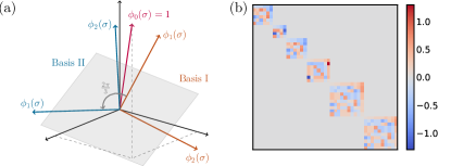
Let us first motivate the search for a basis-agnostic representation of a CE from a geometric observation. By virtue of their aforementioned properties, it follows that standard site basis sets are related by rotations about the hyperplane normal to the constant function . This observation is illustrated graphically for a ternary site space in Figure 1a. Any standard site basis must include two orthogonal basis functions that lie on the plane orthogonal to . The geometry of standard site bases implies that the change of basis matrix (CBM) between two resulting Fourier cluster basis sets is given by products of site basis rotations,
| (4) |
where and are multi-indices for two Fourier cluster basis sets.
The CBM is block-diagonal—any term connecting cluster functions of symmetrically distinct clusters are zero. Further, since the CBM is also unitary, it follows that the blocks themselves are unitary, implying that the norm of expansion coefficients within each block is conserved. A visualization of the block-diagonal CBM between two Fourier cluster bases of a ternary system including up to quadruplet terms is shown in Figure 1b.
To continue, we define reduced correlation functions as the average of cluster functions over symmetrically equivalent contracted multi-indices ,
| (5) |
where is a set (orbit) of symmetrically equivalent contracted multi-indices , i.e. symmetrically equivalent site function permutations over a fixed cluster of sites . is the total number of contracted multi-indices in .
Using reduced correlation functions we rewrite Equation 1 as follows,
| (6) |
where are orbits of symmetrically equivalent clusters of sites ; and are sets of orbits of contracted multi-indices , which represent symmetrically distinct labelings over the sites in the clusters .
The two inner sums in Equation 6 are independent and can be re-arranged to obtain a far more physically intuitive many-body expansion as follows,
| (7) |
where the -body terms account for the energy originating from the interactions amongst the species residing on the clusters . For clusters with more than one site, , we call these terms cluster interactions.
Following the original CE formalism, Equation 7 can also be written as a density by using averages of cluster interactions over symmetrically equivalent clusters ,
| (8) |
we will refer to the terms with for all as mean cluster interactions, and as composition effects for point clusters ().
Equations 7 and 8 are the cluster decomposition of the Hamiltonian . Note that although such an expression can be obtained for any choice of site basis—orthogonal or not—a true cluster decomposition is obtained from a Fourier CE only. This distinction is fundamental since CE expansions using non-orthogonal basis sets will not have the analytical properties that we describe in the remainder of this letter.
It follows directly from our previous analysis of the geometry of Fourier cluster functions, that cluster interactions are invariant to a change of standard basis, i.e. they are invariant to arbitrary rotations orthogonal to . As a result, the norm of the cluster interactions,
| (9) |
is invariant to the choice of standard site basis. In line with CE and discrete Fourier expansion terminology, we will call the squared norm of a cluster interaction the effective cluster weight of a cluster . In addition, we define the total cluster weight as the effective cluster weight multiplied by the multiplicity of its orbit, .
Cluster interactions have the following significant mathematical properties 222Derivations and proofs are given in the Supplemental Material:
-
1.
(zero mean)
-
2.
for (orthogonal)
-
3.
for any set of orbits such that and any function that can be expanded using Fourier basis functions with for . (irreducible)
From properties (1) and (2) it follows that the cluster decomposition of is unique [40]; meaning there exists one and only one set of cluster interactions for any given Hamiltonian . Equivalently, property (1) implies that Equations 7 and 8 are ANOVA-representations of [36, 40]. In fact, re-written in such a form, a CE using a standard basis is nothing more than an fANOVA representation, in which by symmetry, interactions among equivalent clusters are given by the same function . By this consideration, using a cluster decomposition as an effective Hamiltonian to define a Boltzmann distribution can be thought of as log-density ANOVA estimation of a probabilistic graphical model [41, 42, 43].
Using the construction of ANOVA representations, we can now obtain a much deeper understanding of the terms in a CE. Precisely, ANOVA terms are constructed from hierarchical inclusion-exclusion of means conditioned on the occupancy of clusters. For example, it is already known from the original CE formalism [10] that the constant term is equal to the mean of the Hamiltonian. . In the statistics literature, is usually referred to as the grand mean [44]. The single site terms terms, are the difference between the mean conditioned on the -th site and the grand mean, . The point terms of an ANOVA representation are called main effects [44]. The main effects are the mean contribution that a specific species residing on the -th site has on the total energy. The average of main effects in the cluster decomposition (a term in Equation 8) represents the portion of the Hamiltonian that depends on composition only.
The remaining terms involving clusters with more than one site are known as interactions [44], motivating our terminology. A cluster interaction of cluster is computed as the mean conditioned on the sites in cluster , minus the cluster interactions of all its sub-clusters ,
| (10) |
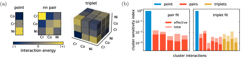
Equation 10 clarifies the meaning of a cluster interaction as the average contribution to the total energy coming solely from a single cluster and none of its subclusters. Accordingly, we see that the terms in the cluster decomposition represent energetic interactions among species occupying the sites of a cluster that are not captured by any lower-order interactions. Figure 2a shows a visualization of the main effect, nearest neighbor pair, and a triplet cluster interactions as Cartesian tensors for a cluster decomposition of a \chCrCoNi alloy.
In our presentation so far, we started with a representation of a cluster decomposition using a CE with a standard basis. However, since the cluster decomposition is basis agnostic, we can discard the concept of a basis altogether. In fact, in the fANOVA and related literature, a function is simply decomposed into its ANOVA representation by directly appealing to Equation 10 [36, 40]. This approach has been used in concurrent work [45], presenting an axiomatic exposition of the cluster expansion and the cluster decomposition, which is in essence equivalent to the formalism of tensor product fANOVA decompositions [42].
As the name analysis of variance suggests, a cluster decomposition also comprises a decomposition of the variance of a Hamiltonian under the a-priori non-interacting product measure [40],
| (11) | ||||
| (12) |
where we used the fact that the variance of each cluster interaction is equal to its cluster weight . Further by using Equation 10, we see that the effective cluster weights are the associated conditional variance with all lower order variances subtracted, i.e. the variance that can be attributed to a single cluster only and to none of its sub-clusters,
| (13) |
Apart from providing a formal characterization of expansion terms, the cluster decomposition provides motivation and interpretations for the choice of regularization used when fitting. For example, Ridge regularization can be interpreted as setting an upper cutoff to the total variance. The use of Tikhonov regularization can be used as a way to more finely set variance cutoffs for specific cluster interaction terms. Recently proposed group-wise regularization [11], can be directly motivated as a judicious form to regularize cluster interactions by weighing coefficients with their permutation multiplicities . Finally, estimation algorithms with hierarchical inclusion/exclusion of clusters [13, 46, 47, 48, 11], can be motivated by appealing to statistical concepts of hierarchically well-formulated models [49] that satisfy marginality constraints [50], or that abide by heredity principles which satisfy either strong or weak hierarchy constraints [51, 52].
In addition, the cluster decomposition allows one to formally rank the importance of the contribution of each cluster interaction following the prescription of Sobol’s sensitivity indices [36]. Accordingly, we define the effective cluster sensitivity index as the fraction of the total variance of carried by the interactions of a cluster ,
| (14) |
Similarly, we define the cluster sensitivity index as the normalized fraction of the total variance of contributed by the cluster interaction of all clusters , per normalizing unit. Cluster sensitivity indices provide a mathematically formal route for evaluating trends in the strength of interactions. Cluster sensitivity indices can be directly computed from a CE by using Equations 9 for the cluster weights. Figure 2b shows cluster sensitivity indices for the interactions of two fitted cluster decompositions of a \chCrCoNi alloy.
As a basic example demonstrating practical use cases of the cluster decomposition, we fit two cluster expansions of a \chCrCoNi medium entropy alloy. Our approach follows a recent study of the \chCrCoNi alloy [34] using a cluster expansion and Wang-Landau sampling [53]. Following previous work, we fit two expansions [34]: a less accurate expansion (in terms of cross-validation error) that includes pairs terms only (pair fit), and a more accurate expansion including pairs and triplets (triplet fit). We only reproduce previous results as an illustration and do not attempt to make any novel scientific claims about this particular alloy.
The energy contributions from interactions of specific species can be obtained by directly inspecting cluster interactions. Figure 2a shows the main effect, pair, and triplet cluster interactions included in the triplet-fit cluster decomposition. We can readily determine which interactions are favorable (negative) and which are unfavorable (positive) based on the color map. The relative trend of the nearest-neighbor interactions obtained directly from the cluster decomposition agrees with previous results obtained via an ad-hoc, over-complete and less accurate nearest-neighbor pair model [34].
The interactions shown in Figure 2a are of different orders of magnitude: the main effect contributions are of eV magnitude, and higher degree interactions are of meV magnitude. We can identify the most important cluster interactions, rank their importance, and compare different fits on rigorous grounds by using the corresponding cluster sensitivity indices as shown in Figure 10b. In both fits, the first two pair interactions are the most important (largest sensitivity), with significant contributions coming from triplet interactions in the triplet fit.
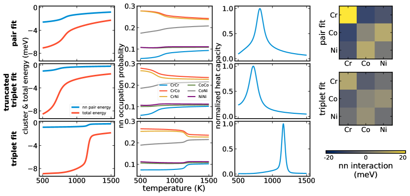
As a further illustration of insights that can be obtained from the cluster decomposition, we computed nearest-neighbor pair short-range order, internal energy, and heat capacity of the \chCrCoNi alloy from an equiatomic canonical Wang-Landau density of states using a 216 atom supercell. Figure 3 shows the computed values for the pair fit and the triplet fit, as well as a truncated expansion including only the pair interactions from the triplet fit (triplet interactions removed). Comparing the nearest-neighbor pair energies and SRO results in Figure 3 of the two decompositions that include only pair interactions, we observe that the overall SRO and total internal energy trends are set predominantly by the first and second nearest neighbor pair interactions (those with the highest cluster sensitivity from Figure 2b). However, based on the triplet fit, we can conclude that triplet terms reduce the fraction of energy attributed to pair terms, tune the SRO values and raise the transition temperature. To delve deeper, one could inspect the triplet interaction values to better understand their role in tuning the ordering transition. These results agree with those reported previously [34], however, by using the cluster decomposition, we have shown how the results can be substantiated with a mathematically formal analysis.
We believe that substantially more insight, use cases, and parameter estimation methods beyond what has been presented here can be developed using the cluster decomposition and its formal statistical properties. The statistical literature is ripe with analysis techniques and methodology—such as log-density ANOVA models [42, 43] and sensitivity analysis [36, 54]—that can be directly leveraged in applications using parameterized lattice models. Several methods already exist in the statistics literature that can be used for direct estimation of cluster interactions and cluster indices in fully basis-agnostic manners [36, 41, 43, 54]. Moreover, the formalism of the cluster decomposition is not limited to scalar functions of discrete degrees of freedom as presented here. In fact, a cluster decomposition can be obtained for any representation of scalar, vector, or tensor-valued function over a tensor product space domain by following the same prescription we have presented. Thus related expansions and generalizations [17, 19, 19, 22] can be suitably recast as cluster decompositions and thus open the door to continued and significant developments based on rigorously established mathematical and statistical grounds.
An implementation of the cluster decomposition and all code used in this work is available at Ref [55].
Acknowledgements.
This work was primarily funded by the U.S. Department of Energy, Office of Science, Office of Basic Energy Sciences, Materials Sciences and Engineering Division under Contract No. DE-AC02-05-CH11231 (Materials Project program KC23MP). This research also used resources of the National Energy Research Scientific Computing Center (NERSC), a U.S. Department of Energy Office of Science User Facility located at Lawrence Berkeley National Laboratory, operated under Contract No. DE-AC02-05CH11231 using NERSC award BES-ERCAP0020531.References
- Hart et al. [2021] G. L. W. Hart, T. Mueller, C. Toher, and S. Curtarolo, Machine learning for alloys, Nature Reviews Materials 6, 730 (2021).
- Sutton and Levchenko [2020] C. Sutton and S. V. Levchenko, First-Principles Atomistic Thermodynamics and Configurational Entropy, Frontiers in Chemistry 8 (2020).
- Nataraj et al. [2021] C. Nataraj, E. J. L. Borda, A. van de Walle, and A. Samanta, A systematic analysis of phase stability in refractory high entropy alloys utilizing linear and non-linear cluster expansion models, Acta Materialia 220, 117269 (2021).
- Xu and Jiang [2019] X. Xu and H. Jiang, Cluster expansion based configurational averaging approach to bandgaps of semiconductor alloys, The Journal of Chemical Physics 150, 034102 (2019).
- Han et al. [2022] G. Han, I. W. Yeu, K. H. Ye, C. S. Hwang, and J.-H. Choi, Atomistic prediction on the composition- and configuration-dependent bandgap of Ga(As,Sb) using cluster expansion and ab initio thermodynamics, Materials Science and Engineering: B 280, 115713 (2022).
- Richards et al. [2016] W. D. Richards, Y. Wang, L. J. Miara, J. C. Kim, and G. Ceder, Design of Li1+2xZn1-xPS4, a new lithium ion conductor, Energy & Environmental Science 9, 3272 (2016).
- Deng et al. [2020] Z. Deng, G. Sai Gautam, S. K. Kolli, J.-N. Chotard, A. K. Cheetham, C. Masquelier, and P. Canepa, Phase Behavior in Rhombohedral NaSiCON Electrolytes and Electrodes, Chemistry of Materials 32, 7908 (2020).
- Van der Ven et al. [2020] A. Van der Ven, Z. Deng, S. Banerjee, and S. P. Ong, Rechargeable Alkali-Ion Battery Materials: Theory and Computation, Chemical Reviews 10.1021/acs.chemrev.9b00601 (2020).
- Chen et al. [2021] B. W. J. Chen, L. Xu, and M. Mavrikakis, Computational Methods in Heterogeneous Catalysis, Chemical Reviews 121, 1007 (2021).
- Sanchez et al. [1984] J. M. Sanchez, F. Ducastelle, and D. Gratias, Generalized cluster description of multicomponent systems, Physica A: Statistical Mechanics and its Applications 128, 334 (1984).
- Barroso-Luque et al. [2022a] L. Barroso-Luque, P. Zhong, J. H. Yang, F. Xie, T. Chen, B. Ouyang, and G. Ceder, Cluster expansions of multicomponent ionic materials: Formalism and methodology, Physical Review B 106, 144202 (2022a).
- Xie et al. [2022] J.-Z. Xie, X.-Y. Zhou, and H. Jiang, Perspective on optimal strategies of building cluster expansion models for configurationally disordered materials, The Journal of Chemical Physics 157, 200901 (2022).
- van de Walle and Ceder [2002] A. van de Walle and G. Ceder, Automating first-principles phase diagram calculations, Journal of Phase Equilibria 23, 348 (2002).
- Van der Ven et al. [2018] A. Van der Ven, J. Thomas, B. Puchala, and A. Natarajan, First-Principles Statistical Mechanics of Multicomponent Crystals, Annual Review of Materials Research 48, 27 (2018).
- Wu et al. [2019] D. Wu, L. Wang, and P. Zhang, Solving Statistical Mechanics Using Variational Autoregressive Networks, Physical Review Letters 122, 080602 (2019).
- Damewood et al. [2022] J. Damewood, D. Schwalbe-Koda, and R. Gómez-Bombarelli, Sampling lattices in semi-grand canonical ensemble with autoregressive machine learning, npj Computational Materials 8, 1 (2022).
- Drautz and Fähnle [2004] R. Drautz and M. Fähnle, Spin-cluster expansion: Parametrization of the general adiabatic magnetic energy surface with ab initio accuracy, Physical Review B 69, 104404 (2004).
- Singer et al. [2011] R. Singer, F. Dietermann, and M. Fähnle, Spin Interactions in bcc and fcc Fe beyond the Heisenberg Model, Physical Review Letters 107, 017204 (2011).
- Thomas and Van der Ven [2017] J. C. Thomas and A. Van der Ven, The exploration of nonlinear elasticity and its efficient parameterization for crystalline materials, Journal of the Mechanics and Physics of Solids 107, 76 (2017).
- Thomas et al. [2018] J. C. Thomas, J. S. Bechtel, and A. Van der Ven, Hamiltonians and order parameters for crystals of orientable molecules, Physical Review B 98, 094105 (2018).
- van de Walle [2008] A. van de Walle, A complete representation of structure–property relationships in crystals, Nature Materials 7, 455 (2008).
- Drautz [2020] R. Drautz, Atomic cluster expansion of scalar, vectorial, and tensorial properties including magnetism and charge transfer, Physical Review B 102, 024104 (2020), arXiv:2003.00221 .
- Drautz [2019] R. Drautz, Atomic cluster expansion for accurate and transferable interatomic potentials, Physical Review B 99, 014104 (2019).
- Ceccherini-Silberstein et al. [2018] T. Ceccherini-Silberstein, F. Scarabotti, and F. Tolli, Discrete Harmonic Analysis: Representations, Number Theory, Expanders, and the Fourier Transform, Cambridge Studies in Advanced Mathematics (Cambridge University Press, Cambridge, 2018).
- Wolverton and Zunger [1995] C. Wolverton and A. Zunger, Ising-like Description of Structurally Relaxed Ordered and Disordered Alloys, Physical Review Letters 75, 3162 (1995).
- BRUSH [1967] S. G. BRUSH, History of the Lenz-Ising Model, Reviews of Modern Physics 39, 883 (1967).
- Sanchez [1993] J. M. Sanchez, Cluster expansions and the configurational energy of alloys, Physical Review B 48, 14013 (1993).
- Sanchez [2010] J. M. Sanchez, Cluster expansion and the configurational theory of alloys, Physical Review B 81, 224202 (2010).
- Stampfl et al. [1999] C. Stampfl, H. J. Kreuzer, S. H. Payne, H. Pfnür, and M. Scheffler, First-Principles Theory of Surface Thermodynamics and Kinetics, Physical Review Letters 83, 2993 (1999).
- Drautz and Díaz-Ortiz [2006] R. Drautz and A. Díaz-Ortiz, Obtaining cluster expansion coefficients in ab initio thermodynamics of multicomponent lattice-gas systems, Physical Review B 73, 224207 (2006).
- Zhang and Sluiter [2016] X. Zhang and M. H. F. Sluiter, Cluster Expansions for Thermodynamics and Kinetics of Multicomponent Alloys, Journal of Phase Equilibria and Diffusion 37, 44 (2016).
- Barroso-Luque et al. [2021] L. Barroso-Luque, J. H. Yang, and G. Ceder, Sparse expansions of multicomponent oxide configuration energy using coherency and redundancy, Physical Review B 104, 224203 (2021).
- Kim et al. [2022] N. Kim, B. J. Blankenau, T. Su, N. H. Perry, and E. Ertekin, Multisublattice cluster expansion study of short-range ordering in iron-substituted strontium titanate, Computational Materials Science 202, 110969 (2022).
- Pei et al. [2020] Z. Pei, R. Li, M. C. Gao, and G. M. Stocks, Statistics of the NiCoCr medium-entropy alloy: Novel aspects of an old puzzle, npj Computational Materials 6, 1 (2020).
- Note [1] The number of distinct basis in lattice gas CE sets grows with the number of components. In a Fourier CE there are infinitely many basis set choices for 3 or more components. In an overcomplete representation [32] there are infinitely many expansion coefficient choices that represent a given Hamiltonian.
- Sobol′ [2001] I. M. Sobol′, Global sensitivity indices for nonlinear mathematical models and their Monte Carlo estimates, Mathematics and Computers in Simulation The Second IMACS Seminar on Monte Carlo Methods, 55, 271 (2001).
- Hoeffding [1948] W. Hoeffding, A Class of Statistics with Asymptotically Normal Distribution, The Annals of Mathematical Statistics 19, 293 (1948).
- Efron and Stein [1981] B. Efron and C. Stein, The Jackknife Estimate of Variance, The Annals of Statistics 9, 586 (1981).
- Note [2] Derivations and proofs are given in the Supplemental Material.
- Hooker [2007] G. Hooker, Generalized Functional ANOVA Diagnostics for High-Dimensional Functions of Dependent Variables, Journal of Computational and Graphical Statistics 16, 709 (2007).
- Jeon and Lin [2006] Y. Jeon and Y. Lin, An Effective Method for High-Dimensional Log-Density Anova Estimation, with Application to Nonparametric Graphical Model Building, Statistica Sinica 16, 353 (2006).
- Jeon [2012] Y. Jeon, A Characterization of the Log-Density Smoothing Spline ANOVA Model, Communications in Statistics - Theory and Methods 41, 2081 (2012).
- Gu [2013] C. Gu, Regression with Responses from Exponential Families, in Smoothing Spline ANOVA Models, Springer Series in Statistics, edited by C. Gu (Springer, New York, NY, 2013) pp. 175–214.
- Gelman [2005] A. Gelman, Analysis of variance—why it is more important than ever, The Annals of Statistics 33, 1 (2005).
- Lammert and Crespi [2022] P. E. Lammert and V. H. Crespi, Cluster expansion methods from physical concepts (2022), ””.
- Zarkevich and Johnson [2004] N. A. Zarkevich and D. D. Johnson, Reliable First-Principles Alloy Thermodynamics via Truncated Cluster Expansions, Physical Review Letters 92, 255702 (2004).
- Leong and Tan [2019] Z. Leong and T. L. Tan, Robust cluster expansion of multicomponent systems using structured sparsity, Physical Review B 100, 134108 (2019).
- Zhong et al. [2022] P. Zhong, T. Chen, L. Barroso-Luque, F. Xie, and G. Ceder, An -norm regularized regression model for construction of robust cluster expansions in multicomponent systems, Physical Review B 106, 024203 (2022).
- Peixoto [1990] J. L. Peixoto, A Property of Well-Formulated Polynomial Regression Models, The American Statistician 44, 26 (1990).
- McCullagh and Nelder [2019] P. McCullagh and J. A. Nelder, Generalized Linear Models, 2nd ed. (Routledge, New York, 2019).
- Hamada and Wu [1992] M. Hamada and C. F. J. Wu, Analysis of Designed Experiments with Complex Aliasing, Journal of Quality Technology 24, 130 (1992).
- Chipman [1996] H. Chipman, Bayesian Variable Selection with Related Predictors, The Canadian Journal of Statistics / La Revue Canadienne de Statistique 24, 17 (1996).
- Wang and Landau [2001] F. Wang and D. P. Landau, Efficient, Multiple-Range Random Walk Algorithm to Calculate the Density of States, Physical Review Letters 86, 2050 (2001).
- Iooss and Lemaître [2015] B. Iooss and P. Lemaître, A Review on Global Sensitivity Analysis Methods, in Uncertainty Management in Simulation-Optimization of Complex Systems: Algorithms and Applications, Operations Research/Computer Science Interfaces Series, edited by G. Dellino and C. Meloni (Springer US, Boston, MA, 2015) pp. 101–122.
- Barroso-Luque et al. [2022b] L. Barroso-Luque, J. H. Yang, F. Xie, T. Chen, R. L. Kam, Z. Jadidi, P. Zhong, and G. Ceder, Smol: A Python package for cluster expansions and beyond, Journal of Open Source Software 7, 4504 (2022b).
- Note [3] Extending to the general case with different site spaces is straightforward.
- Note [4] Which means that site basis functions are uncorrelated under a probabilistic interpretation.
- Kresse and Furthmüller [1996] G. Kresse and J. Furthmüller, Efficiency of ab-initio total energy calculations for metals and semiconductors using a plane-wave basis set, Computational Materials Science 6, 15 (1996).
- Kresse and Joubert [1999] G. Kresse and D. Joubert, From ultrasoft pseudopotentials to the projector augmented-wave method, Physical Review B 59, 1758 (1999).
- Perdew et al. [1996] J. P. Perdew, K. Burke, and M. Ernzerhof, Generalized Gradient Approximation Made Simple, Physical Review Letters 77, 3865 (1996).
- Jain et al. [2013] A. Jain, S. P. Ong, G. Hautier, W. Chen, W. D. Richards, S. Dacek, S. Cholia, D. Gunter, D. Skinner, G. Ceder, and K. A. Persson, Commentary: The Materials Project: A materials genome approach to accelerating materials innovation, APL Materials 1, 011002 (2013).
- Ong et al. [2013] S. P. Ong, W. D. Richards, A. Jain, G. Hautier, M. Kocher, S. Cholia, D. Gunter, V. L. Chevrier, K. A. Persson, and G. Ceder, Python Materials Genomics (pymatgen): A robust, open-source python library for materials analysis, Computational Materials Science 68, 314 (2013).