Screening Methods for Classification Based on Non-parametric Bayesian Tests

Abstract: Feature or variable selection is a problem inherent to large data sets. While many methods have been proposed to deal with this problem, some can scale poorly with the number of predictors in a data set. Screening methods scale linearly with the number of predictors by checking each predictor one at a time, and are a tool used to decrease the number of variables to consider before further analysis or variable selection. For classification, there is a variety of techniques. There are parametric based screening tests, such as $t$-test or SIS based screening, and non-parametric based screening tests, such as Kolmogorov distance based screening [Mai and Zou, 2012], and MV-SIS [Cui et al., 2015]. We propose a method for variable screening that uses Bayesian-motivated tests, compare it to SIS based screening, and provide example applications of the method on simulated and real data. It is shown that our screening method can lead to improvements in classification rate. This is so even when our method is used in conjunction with a classifier, such as DART, which is designed to select a sparse subset of variables. Finally, we propose a classifier based on kernel density estimates that in some cases can produce dramatic improvements in classification rates relative to DART.

Keywords: Independent Screening, Variable Selection, Classification, Bayes Factors

1 Introduction

Classification involves predicting a class label for an observation, given a set of predictor variables. The techniques for doing so are wide ranging, including support vector machines [Boser et al., 1992], tree based methods [Brieman et al., 1984], Bayesian trees [Linero and Yang, 2018] and gradient boosting trees [Friedman, 2002].

It is common to encounter a data set with many features, but rarely are all of them important. Picking a subset of these features quickly is a task that is desired, but can be tricky for very large data sets. Removing unimportant variables can result in dramatic improvement for some of the previously mentioned classification methods. Feature selection is not a new field, and can be divided into three categories: screening or filter based methods, wrapper methods, and embedded methods [Tang et al., 2014]. Screening methods examine each variable one at a time to see if it provides useful information, and as a result scale linearly with the number of predictors. However, examining each variable individually can cause information on joint behavior of variables to be lost, or can cause collinear variables to be selected [Tang et al., 2014]. Wrapper methods fit different models, and then evaluate each one according to some criterion. The model that does best according to this criterion is selected. While this tends to select good variable subsets, fitting every model can be extremely time-consuming, especially if the data set is very large [Tang et al., 2014]. Embedding methods produce a model that has some sparsity built into it, producing a set of useful variables and a model built with them, simultaneously. The speed of different embedding methods varies with the strategy used to obtain sparsity, but these are typically slower than screening methods [Tang et al., 2014].

Our focus in this paper will be on screening methods. It is a common strategy to employ a screening method and then employ an embedding method (such as LASSO) afterwards. Fan [Fan and Lv, 2008] employs this strategy and improves both the time it takes to run LASSO and the accuracy of the model as a whole. Since then several filter methods have popped up. For classification in particular, maximum marginal likelihood screening [Fan et al., 2010], MV-SIS [Cui et al., 2015], and Kolmogorov distance screening [Mai and Zou, 2012] are some of the screening tests that have been published. Most of these methods are applied to linear discriminant analysis and show improvement in applying these methods to a data set after the screening has been performed. This paper proposes a new screening method when the number of classes is known to be two, and show that it results in improved classification accuracy in settings where the simple model underlying linear discriminant analysis does not hold. Our screening method identifies informative features by using a two-sample Bayesian test that checks whether two data sets share the same distribution[Merchant and Hart, 2022]. One of our goals is to show that classification methods, including BART [Linero and Yang, 2018], DART [Linero and Yang, 2018] and SVM [Boser et al., 1992], can be improved when preceded by our screening procedure.

2 Methodology

Our screening method is based on computing a statistic for each individual feature. We will use kernel density estimates of the two distributions corresponding to the two classes. The idea is similar to that of Kolmogorov distance screening: if it seems likely that the two classes have different distributions for a feature, then we will keep the feature. We define a test statistic that can make this determination.

Suppose we observe the data $X$, an $(m+n)\times p$ matrix whose $i$th row, $(X_{i1},\ldots,X_{ip})$, contains the values of the $p$ variables for one subject. The $i$th element, $Y_{i}$, of vector $Y$ is 0 or 1 and indicates the class to which the $i$th subject belongs, $i=1,\ldots,m+n$. For now, suppose that $Y_{1},\ldots,Y_{n}$ are $0$ and $Y_{n+1},\ldots,Y_{n+m}$ are $1$. We have $n+m$ data vectors and $p$ features. Consider the data $\mbox{\boldmath$X$}_{j}=(X_{1j},\ldots,X_{(m+n)j})$ for feature $j$ and define $\hat{h}_{i}(\cdot|\mbox{\boldmath$X$}_{j},b)$ to be a kernel density estimate that has bandwidth $b$ and uses all the data in $\mbox{\boldmath$X$}_{j}$ except that of the $i$th subject:

$$\hat{h}_{i}(x|\mbox{\boldmath$X$}_{j},b)=\frac{1}{nb}\sum_{\begin{subarray}{c}r=1\\ r\neq i\end{subarray}}^{n+m}K\left(\frac{x-X_{rj}}{b}\right).$$

We also compute kernel estimates from the data sets consisting of observations where $Y=0$ and $Y=1$. These are

$$\hat{f}_{i}(\cdot|\mbox{\boldmath$X$}_{j},b)=\frac{1}{nb}\sum_{\begin{subarray}{c}r=1\\ r\neq i\end{subarray}}^{n}K\left(\frac{x-X_{rj}}{b}\right)$$

and

$$\hat{g}_{i}(\cdot|\mbox{\boldmath$X$}_{j},b)=\frac{1}{nb}\sum_{\begin{subarray}{c}r=n+1\\ r\neq i\end{subarray}}^{n+m}K\left(\frac{x-X_{rj}}{b}\right).$$

Then we define the test statistics $ALB_{j}$, $j=1,\ldots,p$:

$$(m+n)ALB_{j} = \sum_{i=n+1}^{m}\text{log}\left(\frac{\hat{g}_{i}(X_{ij}|\mbox{\boldmath$X$}_{j},b)}{\hat{h}_{i}(X_{ij}|\mbox{\boldmath$X$}_{j},b)}\right)+\sum_{i=1}^{n}\text{log}\left(\frac{\hat{f}_{i}(X_{ij}|\mbox{\boldmath$X$}_{j},b)}{\hat{h}_{i}(X_{ij}|\mbox{\boldmath$X$}_{j},b)}\right)$$

$$\mathrel{\stackrel{{\scriptstyle\makebox[0.0pt]{\mbox{\tiny def}}}}{{=}}} \sum_{i=n+1}^{m}\text{log}(B_{1ji})+\sum_{i=1}^{n}\text{log}(B_{2ji}).$$

The notation $ALB$ stands for Average Log-Bayes factor, since, as argued by [Merchant and Hart, 2022], the statistics $B_{1jr}$ and $B_{2js}$ are Bayes factors based on the data “sets” $X_{rj}$ and $X_{sj}$, respectively. We refer to [Merchant and Hart, 2022] for a thorough exploration of such average log-Bayes factors.

Another motivation for $ALB_{j}$ is in terms of Kullback-Leibler divergence, which for densities $h_{1}$ and $h_{2}$ is

$$KL(h_{1},h_{2})=\int_{-\infty}^{\infty}h_{1}(x)\log\left(\frac{h_{1}(x)}{h_{2}(x)}\right)\,dx.$$

Define $f_{j,{\rm mix}}=(nf_{j}+mg_{j})/(n+m)$, where $f_{j}$ and $g_{j}$ are the densities of feature $j$ for classes 0 and 1, respectively. Then the statistic $ALB_{j}$ is an approximately unbiased estimator of the following quantity:

$$\left(\frac{n}{m+n}\right)KL\left(f_{j},f_{j,{\rm mix}}\right)+\left(\frac{m}{m+n}\right)KL\left(g_{j},f_{j,{\rm mix}}\right).$$

In the case $f\equiv g$, $ALB_{j}$ converges to 0 in probability as $m$ and $n$ tend to $\infty$. The null distribution of $ALB_{j}$ can be assessed using a permutation-based procedure to determine if two sets of observations arise from a common distribution.

[Merchant and Hart, 2022] propose selecting the bandwidth $b$ by leave-one-out cross validation, a proposal that tacitly assumes the null hypothesis to be true. While this strategy has potential, we believe it to be too computationally expensive to use for every variable separately. We only have to do this $p$ times, suggesting linear scaling with the variable length, but this introduces quadratic scaling with $n$, which is prohibitive for large data sets. Instead, we opt to use a normal plug-in bandwidth in conjunction with the heavy tailed Hall kernel, which is:

$$K_{0}(z)=\frac{1}{\sqrt{8\pi e}\,\Phi(1)}\exp\left[-\frac{1}{2}(\log(1+|z|))^{2}\right].$$

Simulation results show that the constant for the plug-in is $0.162$ to 3 decimal places, resulting in the following plug-in rule for variable $j$:

$$b_{\text{plug-in},j}(\mbox{\boldmath$X$}_{j})=0.162(m+n)^{-1/5}s_{j},$$

where $s_{j}$ is an estimate of the underlying (null) standard deviation. One possibility is to take $s_{j}$ to be the sample standard deviation for $\mbox{\boldmath$X$}_{j}$, but we prefer the more robust choice $s_{Rj}=IQR(\mbox{\boldmath$X$}_{j})/1.35$.

Suppose we have computed $ALB_{1},ALB_{2},ALB_{3},...,ALB_{p}$. The matter still remains in choosing a cutoff for the $ALB$s such that we select all variables with $ALB$ larger than the cutoff. Below are some possible ways of doing so.

• Choose the cutoff to be some percentile of $ALB_{1},ALB_{2},ALB_{3},...,ALB_{p}$. This is in line with what some of the authors in SIS and SIRS propose. Suppose we expect $d$ features to be important in the data set, then we can set our cutoff to be the $100(1-d/p)$th percentile. Clearly, the largest $d$ test statistics are the most likely to be significant. A problem with this approach is selecting an appropriate value for $d$. The authors in SIS [Fan and Lv, 2008] and SIRS [Zhu et al., 2011] argue that a conservative choice for $d$ is $n$ or $n\log(n)$, although these choices seem somewhat arbitrary.

• An empirical but computationally daunting way to approach this problem is to proceed with two training sets and a classification method. We can choose the cutoff that minimizes the error rate of the classification method when it is trained on one of the training sets and then applied to the other. To keep the computational scaling of the procedure linear with $p$, we recommend restricting the number of candidate cutoff values to be fairly small, say no more than ten.

• Randomly select a covariate, say $\mbox{\boldmath$X$}_{j}$. For this covariate, permute the labels, and compute the test statistic, call it $ALB_{1}^{*}$. Using the same feature $\mbox{\boldmath$X$}_{j}$, repeat this procedure $d$ times, resulting in $ALB_{1}^{*},\ldots,ALB_{d}^{*}$. We randomly select $B-1$ more covariates without replacement, and repeat the previous steps for each of them, resulting in a total of $Bd$ values of $ALB$. Once this is done, we choose the cutoff to be a percentile of these $Bd$ values. This method also approximates the null conditional distribution of $ALB$ for a randomly selected feature, but potentially has the advantage of requiring fewer statistics to be computed than in A3.

• The Bayes factor interpretation of $ALB_{j}$ entails that variable $j$ should never survive screening when $ALB_{j}<0$, suggesting that we use 0 as a cutoff. While this choice may seem liberal, [Merchant and Hart, 2022] show that an $ALB$ cutoff of 0 produces a test whose type I error probability tends to 0 as $m+n$ tends to $\infty$.

It should be noted that a particular screening method will work differently with different classifiers, although this is perhaps to be expected. We encourage the use of a classifier that can take advantage of differences in distribution other than location differences. A popular classifier is linear discriminant analysis (LDA), by which we mean the version that assumes equal covariance matrices for the two classes. Features identified as important due to a scale difference between classes will usually be of no use to LDA.

Of the methods A1-A4, the least computationally expensive ones are A1 and A4. Use of these cutoffs also has the advantage of producing a test with power tending to 1 as $m+n$ tends to $\infty$, since $ALB_{j}$ converges to 0 in probability when $f_{j}\equiv g_{j}$ [Merchant and Hart, 2022]. Method A1 is recommended if there is a strong idea as to how many variables are expected to be relevant or if there is a critical number of variables that are needed for another classifier to work well.

Lastly we wish to note that each $ALB$ has a finite upper bound, as it is easily shown that

$$ALB_{j}\leq\log(2)\cdot\max\left(\frac{m}{(m-1)},\frac{n}{(n-1)}\right),$$

which implies that $ALB_{j}$ is essentially bounded by $\text{log}(2)$ so long as $m$ and $n$ are not too small.

3 Consistency results

We begin with the assumption that every variable satisfies conditions A1-A5 in [Merchant and Hart, 2022]. We will also assume that the numbers, $m$ and $n$, of samples for the two classes tend to infinity, and the number of variables, $p$, is fixed. Suppose that a variable belongs to class $D$ if the variable marginally offers information, which means that the variable has a different distribution for one class than it does for the other. Finally, we assume that the variables are independent.

Theorem 1.

If the above assumptions hold, then

$$\lim_{n,m\rightarrow\infty}P(\max_{i\in D^{c}}ALB_{i}<\min_{j\in D}ALB_{j})\rightarrow 1.$$ (1)

Suppose we use a cutoff as in A4 (in our Section 3). Then we also have the following result:

$$\lim_{n,m\rightarrow\infty}P(\min_{j\in D}ALB_{j}>0\cap\max_{j\in D^{c}}ALB_{j}<0)\rightarrow 1.$$ (2)

Proof.  Result (2) implies (1), so we only prove the former. Using the fact that $P(A\,\cap\,B)\geq 1-P(A^{c})-P(B^{c})$, it is enough to show that both $P(\min_{j\in D}ALB_{j}>0)$ and $P(\max_{j\in D^{c}}ALB_{j}<0)$ tend to 1.

We only consider $P(\max_{j\in D^{c}}ALB_{j}<0)$ as the proof for the other probability is similar. We have

$$P(\max_{j\in D^{c}}ALB_{j}<0) = P\left(\bigcap_{j\in D^{c}}\{ALB_{j}<0\}\right)$$ (3)

$$= \prod_{j\in D^{c}}P(ALB_{j}<0)$$

$$\geq \left(\min_{j\in D^{c}}P(ALB_{j}<0)\right)^{N},$$

where $N$ is the number of elements in $D^{c}$. For each $j\in D^{c}$, [Merchant and Hart, 2022] show that $P(ALB_{j}<0)\rightarrow 1$ as $m$ and $n$ tend to $\infty$. Since $N$ is finite, this implies that the quantity on the right-hand side of (3) tends to 1, from which the result follows. $\ \blacksquare$

It is clear that if $p$ tends to $\infty$ at a sufficiently slow rate, then Theorem 1 remains true. However, determining the precise rate at which $p$ can increase relative to $m$ and $n$ requires stronger results than provided by [Merchant and Hart, 2022], and we will not pursue this direction further.

We now show simulation results for various values of $m=n$, $p$ and $r$, where $r$ represents the proportion of important variables, i.e., variables for which the class distributions are different. We generate 500 variables for a binary classification problem in the following fashion. If it is important, the variable is drawn for one class from a $t$-distribution with 4 degrees of freedom, and drawn from the other class from a mixture of two normal distributions, where the mixing parameter is 1/2, the standard deviation of both normal distributions is 1, and the means are -2.5 and 2.5. If instead the variable is unimportant, then it is drawn from a standard normal. We will name the method of generating variables in this setting “a shape difference.” Finally, each variable is determined to be important or not by performing a binomial trial with success probability $r=1/2$. Figures 1, 2, and 3 show how the cdfs of the $ALB$s change depending on $m$ and $n$.

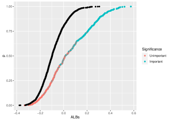
Figure 1: Comparison of ALB CDFs when the training set sizes are equal to 10 and important variables have a shape difference. The black curve denotes the CDF of $ALB$s generated from data where the classes are permuted.

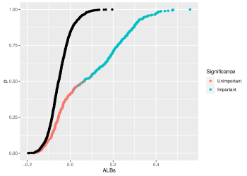
Figure 2: Comparison of ALB CDFs when the training set sizes are equal to 20 and important variables have a shape difference. The black curve denotes the CDF of $ALB$s generated from data where the classes are permuted.

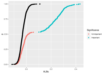
Figure 3: Comparison of ALB CDFs when the training set sizes are equal to 40 and important variables have a shape difference. The black curve denotes the CDF of $ALB$s generated from data where the classes are permuted.

As the sample sizes $m$ and $n$ increase, the $ALB$s for important variables gradually increase. Even when the total number of observations is only eight percent of the total number of variables, we achieve the property that the largest $ALB$ of the unimportant variables is smaller than the smallest $ALB$ of the important variables. The black curve shows the cdf of $ALB$s computed by permuting the labels for each variable three times and computing the $ALB$ each time. A cutoff of 0 is not larger than the largest unimportant variable for any $n$, but is still useful for discarding a large portion of the unimportant variables. On the other hand, using a large percentile of the permuted variables can result in discarding almost all of the unimportant variables, and at the largest sample size, choosing the cutoff to be the maximum of the permuted $ALB$s does indeed almost perfectly separate the important and unimportant variables.

4 Discussion of classification methods

Ideally, one should choose the screening method and classifier that work best together. Good examples of this principle are provided by the relationship that classification methods such as logistic regression, support vector machines, and linear discriminant analysis have with $t$-test based screening. Discriminant analysis, support vector machines without a kernel trick, and logistic regression are designed to take advantage of location differences between classes. It is therefore natural to precede them with $t$-test screening, which, of course, is designed to detect differences between means. On the other hand, support vector machines that use a kernel trick create a hyper-plane that best separates the two classes essentially after a transformation is performed, and can therefore deal effectively with many types of differences between distributions. To take advantage of this ability, it is thus best to use a screening method that can detect non-location differences. In summary, $t$-test screening is a natural method to use when linear discriminant analysis or logistic regression are deemed to be appropriate classifiers, but is not necessarily a good method when a support vector machine with a kernel trick is required. By linear SVM, we mean a method that can classify by separating the two groups by a plane.

In Figures 4 and 5 two (important) variables are generated according to a shape difference. The bimodality of one of the two class distributions makes the classes hard to separate with a plane. Figure 4 shows the performance of a support vector machine when only two relevant variables are used for classification, while Figure 5 shows the improvement in the same situation when the kernel trick is applied to detect non-location based differences.

Our method seeks to outperform $t$-test screening by considering differences other than ones of location type. Of course, this performance is not free. It comes with the cost that we lose some power in detecting differences of means. For our method to work better with a classifier, the classifier must have the ability to distinguish classes that display non-location differences. For example, a set of variables whose classes differ only with respect to scale would not be useful to support vector machines without the kernel trick and LDA, as there would be no hyperplane that nicely separates the classes. A kernel trick or increasing the number of variables by considering interactions and squared terms can sidestep this issue. But adding variables is not ideal, as a goal of our methodology is to decrease computational complexity.

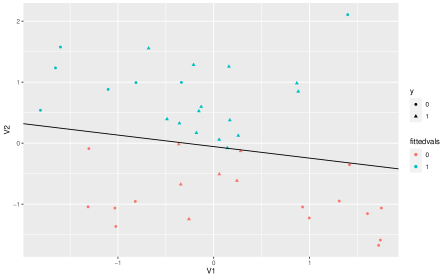
Figure 4: Prediction accuracy of two important variables in the setting of “a shape difference” using a linear SVM. The colors represent the predictions that the SVM produces. The line represents the discriminator that a linear SVM produces to discriminate the classes. The triangle and circle represent which class the observation arises from.

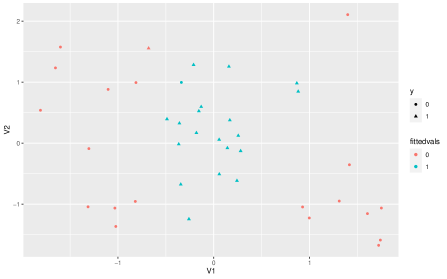
Figure 5: Prediction accuracy of two important variables in the setting of “a shape difference” with an SVM that uses a kernel trick. The colors represent the predictions that the SVM produces when a kernel trick is applied. The triangle and circle represent which class the observation arises from. Classification is much better in this case because the trick enables the classifier to capture differences other than location shifts.

Finally, we would like to add that even though SVM with the kernel trick is a fine classification method that uncovers many different types of differences between variables, its performance can be degraded harshly by the presence of noisy variables. To illustrate this, we use data in the same setting as the shape difference. We constructed a training and testing set such that both consist of 10 observations from each class. Five hundred variables were used, with only 10% on average being important. All data for unimportant variables have a standard normal distribution. If a variable is important, then its distribution in one class is a bimodal mixture of two normals and in the other class a $t$-distribution with 4 degrees of freedom. The normal distributions in the mixture both have standard deviation 1 and means of -2.5 and 2.5. We trained an SVM with the radial basis kernel on all of the observations, and trained another SVM with the radial basis kernel but used only variables whose ALB value was larger than the interpretative cutoff of 0. We repeat this procedure 100 times, and report on its accuracy in Figure 6. In general, classification accuracy is greatly improved, false negatives rarely happen after screening and the number of false positives is reduced.

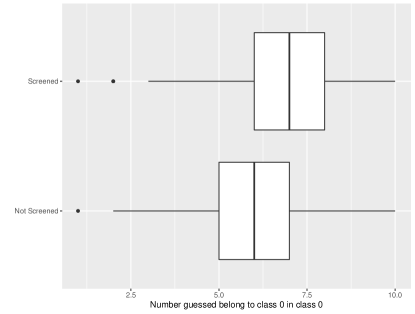
(a) Boxplots of true positives

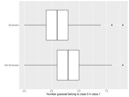
(b) Boxplots of false positives

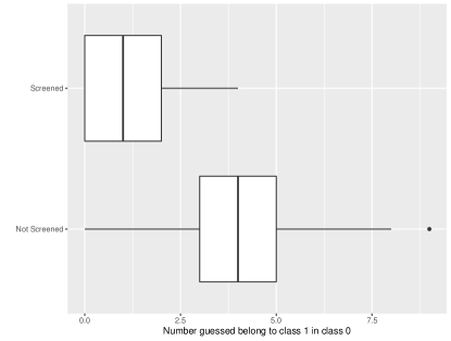
(c) Boxplots of false negatives

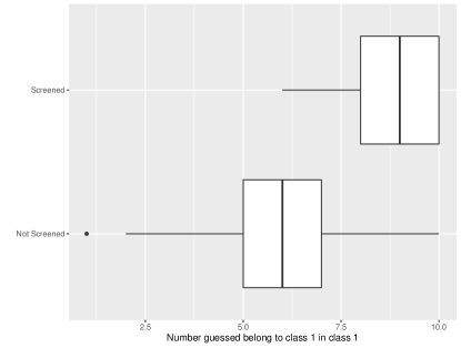
(d) Boxplots of true negatives

Figure 6: Box plots displaying the accuracy of SVM when the data are generated from model where $10\%$ of the variables are important and have a shape difference. To illustrate the accuracy of the methods, we do the following. First, suppose a positive case corresponds to an observation being in class 1 and a negative case corresponds to an observation being in the other class. Then to show the accuracy of the SVMs, we show boxplots on the number of “True Positives,” “True Negatives,” “False Positives” and “False Negative” occurrences.

The ALB screening method need not be the final say as to which variables to include. Two variables that are individually important but highly correlated might be selected, although this may not be ideal for some classifiers. Screening can simply be a precursor that simplifies the job of a classifier, which does further variable selection. Even methods that can perform variable selection and modeling simultaneously can benefit from having the number of variables reduced dramatically by screening. This is observed in SIRS [Zhu et al., 2011], SIS [Fan and Lv, 2008], and is also true in our case.

5 Interaction with BART and a tailored classification method

We have recommended using classification methods that can take advantage of features for which the classes have non-location differences. Methods that do further variable selection or that can handle sparse data sets can also fare quite well with our screening methods. BART and DART are methods having few parametric assumptions and that are able to capture a large variety of features from the data. BART has issues as the number of predictors grow, and DART has been proposed as a solution for this issue [Linero and Yang, 2018]. While DART can handle the case where many predictors are irrelevant, there is a cost. Mixing times of the chains for DART are increased compared to BART, and a prior that encourages sparsity may cause DART to get trapped in a posterior mode when the MCMC procedure to estimate it is run [Hill et al., 2020]. While we cannot directly mitigate these problems, decreasing the number of variables helps speed up the MCMC procedure. Our screening method can decrease the number of variables at a faster rate than DART can. DART is resilient against correlated nuisance variables and can therefore eliminate variables that survive ALB screening but are irrelevant due to collinearity. We provide simulations showing that use of our screening method before BART or DART can result in improved misclassification rates and computing speeds.

We generate data in the same context as Figure 2, but instead roughly 10% of the variables are relevant. If a variable is irrelevant, the distribution of the variable for both classes is standard normal. To assess the performance of a classifier, we computed the Rand index, or the percentage of correct decisions the classifier has made. We compute the Rand index for the BART and DART procedures applied to all variables, and the Rand index of the same procedures applied to variables that survive ALB screening. We consider different training set sizes that vary from 5 to 20. The testing set size for each simulation is the same as the training set size. We repeat this 100 times for each sample size.

Figures 7 and 9 show how accurate BART and DART alone are in these settings and Figures 8 and 10 show how the methods do when variables are screened for importance beforehand. There is a notable gain in the Rand index as the training set size gradually increases for both methods. Of greater note is that the time it takes to run both procedures is decreased. Figure 11 shows the amount of time it takes the BART method to run before screening and Figure 12 shows how long the method takes after screening. Screening on average shaves off at least 10 seconds of computation time while increasing the average accuracy. This is an interesting result, as the methods themselves, DART especially, tend to be robust to irrelevant variables. However, the figures suggest that a larger sample size is required to achieve that robustness.

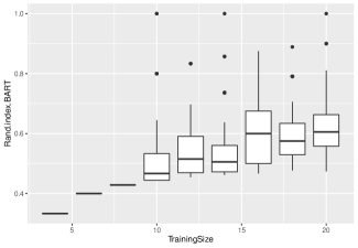
Figure 7: Box plots of the Rand index of BART in the setting of a shape difference. We vary $m$ with $m=n$, and the training size in the plot denotes $m+n$. We repeat each simulation 100 times for each sample size. Roughly 10% of the variables are relevant.

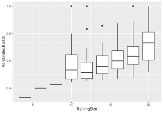
Figure 8: Box plots of the Rand index of BART when BART is improved by screening. This is in the same setting as that used in Figure 7. The difference between the two plots is that we screened the variables with the ALB procedure before applying BART. We choose variables such that all generated ALBs are larger than the interpretable cutoff of 0. The power of the classification method grows large when enough data is accrued. The interpretive cutoff tends to be conservative, and power of the approach is likely to be even larger if a permutation-based cutoff is used instead.

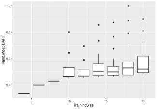
Figure 9: Box plots of the Rand index of DART. This is in the same setting as in Figure 7, with the difference that we use DART instead of BART as it is capable of automatically performing variable selection.

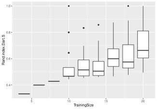
Figure 10: Box plots of the Rand index of DART improved by screening. This is in the same setting as in Figure 7. The difference here is we screen the variables with the ALB procedure before applying DART. We choose variables such that all generated ALBs are larger than 0. The power of the classification method has improved after screening for variables, despite DART being fully capable of automatically performing variable selection automatically.

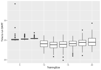
Figure 11: Box plots of the time it took to run DART. The simulation is in the same setting as in Figure 7.

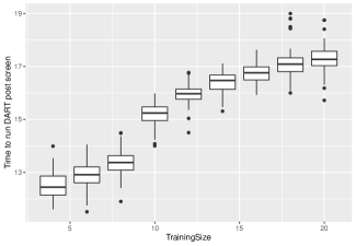
Figure 12: Box plots of the time it took to run DART post screening. This is in the same setting as in Figure 7. The difference here is we screen the variables with the ALB procedure before applying DART. The screening procedure itself takes much less than half a second, and as a result of removing a large number of irrelevant variables, greatly improves the amount of time it takes for DART to run.

5.1 A simple Bayesian classifier

Suppose our goal is to simply leverage the differences between variables, regardless of the type of difference, and that we assume independence between variables. We can construct a simple Bayesian method for classification in the following fashion. For each variable, we compute two kernel density estimates, one for each class. For each variable $i$, let $\hat{f}_{i}$ and $\hat{g}_{i}$ be kernel density estimates using all variable $i$ data from classes 1 and 2, respectively. The prior probability that a variable arises from a class is assumed to be proportional to the number of observations for that class. Let $\mbox{\boldmath$x$}=(x_{1},...,x_{p})$ be an observation to be classified. If the underlying densities are known, then the conditional probability that $x$ came from class 1 is

$$p(\mbox{\boldmath$x$})=P(Y=1|\mbox{\boldmath$x$})=\frac{\frac{n}{m+n}\prod_{i\in D}f_{i}(x_{i})}{\frac{n}{m+n}\prod_{i\in D}f_{i}(x_{i})+\frac{m}{m+n}\prod_{i\in D}g_{i}(x_{i})},$$ (4)

where $D$ is the set of indices $i$ such that $f_{i}\not\equiv g_{i}$. Of course, the densities and $D$ are unknown, but $p(\mbox{\boldmath$x$})$ can be estimated using kernel density estimates, and $D$ can be replaced by $\widehat{D}$, the set of indices such that the corresponding variables survive screening:

$$\hat{p}(\mbox{\boldmath$x$})=\frac{\frac{n}{m+n}\prod_{i\in\widehat{D}}\hat{f_{i}}(x_{i})}{\frac{n}{m+n}\prod_{i\in\widehat{D}}\hat{f_{i}}(x_{i})+\frac{m}{m+n}\prod_{i\in\widehat{D}}\hat{g_{i}}(x_{i})}.$$ (5)

A classifier based on (5) can be a powerful tool for capturing marginal differences in distributions, but is incapable of leveraging differences that may lie in the dependence structure of the variables. To use (5), we say that an observation $x$ belongs to class 1 if $\hat{p}(\mbox{\boldmath$x$})>n/(m+n)$ and to class 2 otherwise. We have found this classifier to have strong accuracy when dealing with independent variables, or with settings where the difference in multivariate distributions is dominated by marginal differences.

To illustrate the effectiveness of the classifier based on (5), we perform a simulation similar to the one referenced in Figure 1 but under a variety of different sample sizes. We repeat this procedure 5 times. For each sample size, we generate a balanced testing set of the same size, and compute a Rand index. A plot of the Rand indices against the sample size is found in Figure 13. The power of the classification method grows to be quite large at even small $m+n$ values. Since the interpretive cutoff tends to be conservative, power of the approach is likely to be even larger if a permutation based cutoff is utilized instead. At a training size of just 9 samples in each group, the classifier makes perfect predictions over 75% of the time.

Figure 13: A box plot of the Rand index of the Bayesian classifier. The classifier is defined in terms of (5). We generate data in the same context as in Figure 2, but vary $m$ and $n$ so that $m=n$, and the training size denotes $m+n$. We choose variables such that all generated ALBs are larger than the intepretable cutoff of $0$.

6 Application on simulated data sets

We want to compare our method to $t$-test screening and also compare performance of the different choices of ALB cutoff. There are at least two ways to go about this. One is to compare the percentage of variables that survive screening from both procedures, and the other is to apply a classification method after screening and see which method has a better classification rate. These procedures are carried out in three cases:

• Case 1 – Location differences. There are 600 variables, and those that are important arise from a case where there is a mean difference between classes. If the variable is important, one class has a standard normal distribution and the other a normal distribution with mean 1 and standard deviation 1. We let roughly $5\%$ of the variables be important by generating 600 independent Bernoulli variables, each with success probability $0.05$. This way of determining important variables is used in Cases 2 and 3 as well. Also, in this case and the following two the unimportant variables have standard normal distributions. The classifier we will use to compare performance in this case is SVM without the kernel trick.

• Case 2 – Scale differences. There are 600 variables, and those that are important arise from a case where there is a variance difference between classes. If the variable is important, one class has a standard normal distribution and the other a normal distribution with mean 0 and standard deviation 3. We let roughly $20\%$ of the variables be important, and the classifier used is the support vector machine with a kernel trick.

• Case 3 – Shape differences. There are 600 variables, and those that are important arise from a case where the class distributions have different shapes. If the variable is important, one class has a standard $t$-distribution with 4 degrees of freedom and the other a bimodal mixture of two normal distributions with means -2.5 and 2.5 and the same standard deviation of 1. Roughly $10\%$ of the variables are important, and the classifier used is the support vector machine with a kernel trick.

For all three cases, screening was done and the classifier built from a training set of $m+n$ observations on each variable, where $m=n$. The classifier so built was applied to predict $m+n$ observations, and the resulting Rand index was calculated. In $t$-test screening, variables were selected when their $P$-values were smaller than $0.005$. We repeated this procedure 100 times for each sample size. Figures 14-16 show, respectively, how well the methods performed for three ways of choosing an ALB cutoff: a “fixed type I error rate” approach, the largest $n+m$ values of ALB, and a cutoff of $0$.

The results of these simulations suggest that ALB screening is effective at detecting location differences, as in Case 1, but not to the same degree as $t$-test screening. In Case 1, the performance of the SVM with ALB screening is better than with no screening, but worse than with $t$-test screening. The proportion of variables that survive ALB screening steadily increases as sample size increases, but at a slower rate than with $t$-test screening. In Cases 2 and 3, $t$-test screening does no better than no screening in terms of classification accuracy. Regarding preservation of important variables, $t$-test screening does not improve as the sample size increases, but ALB screening does.

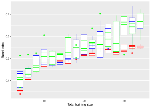
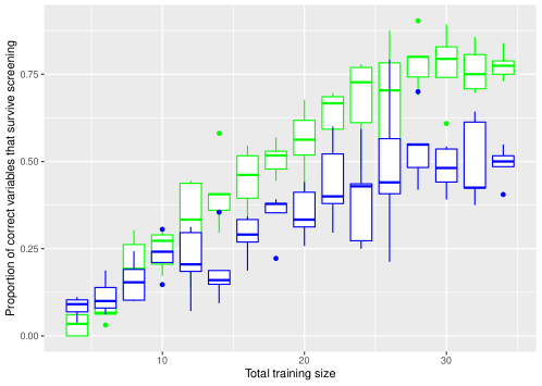
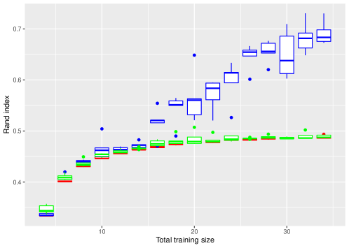
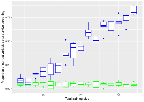
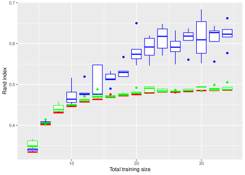
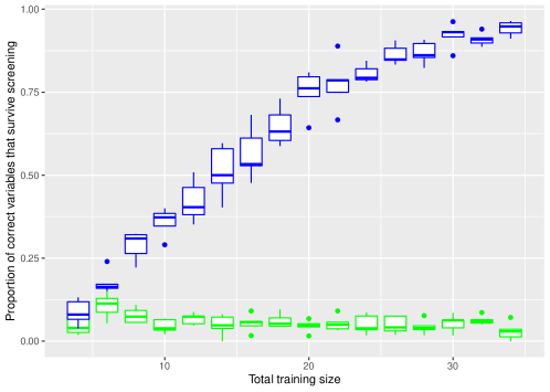
Figure 14: Simulation results for $t$-test screening and ALB screening that uses A3. We generate $ALB^{*}$ values by permuting the data labels and computing $ALB$ for the resulting data. We do this for every variable twice. The ALB cutoff is the $95$th percentile of $ALB^{*}$. The $t$-statistic cutoff is chosen so that the $P$-value is less than $0.05$. Red, green and blue box plots are for no screening, $t$-test screening, and ALB screening, respectively. The first, second and third row of plots correspond to cases 1, 2 and 3, respectively.

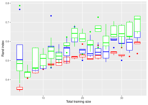
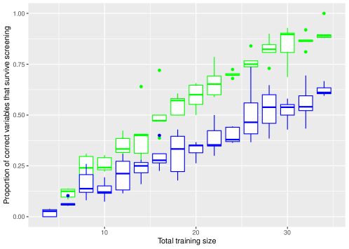
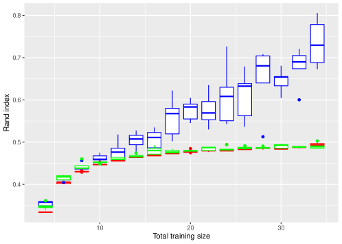
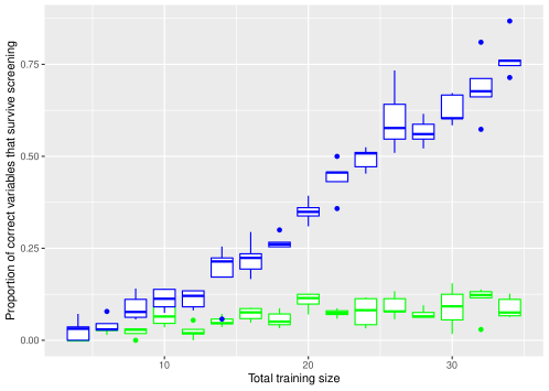
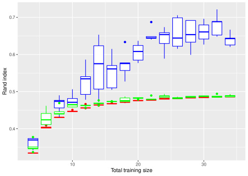
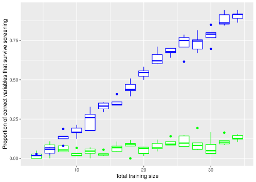
Figure 15: Simulation results for $t$-test screening and ALB screening that uses variables with $n+m$ largest values of ALB. The colors of the box plots have the same meaning as they do in Figure 14.

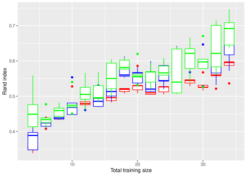
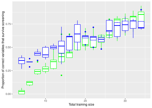
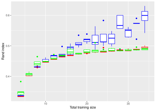
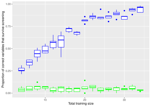
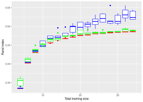
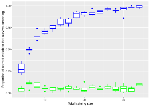
Figure 16: Simulation results for $t$-test screening and ALB screening with cutoff $0$. The colors of the box plots have the same meaning as they do in Figure 14.

7 Application to the GISETTE data

The GISETTE data are obtained from $m=3000$ and $n=3000$ handwritten images of the digits 4 and 9, respectively. For each of the 6000 images, $p=5000$ variables are measured, some of which are irrelevant probes, and the others pixel intensities. We will perform classification on these data, using different screening methods to choose different subsets of the variables. We will rely on DART to be the primary classification method and will explore how it performs when aided by different screening methods.

The data set was randomly split into two halves. The first half was treated as the training data. We trained our classifier and computed $t$-statistics and ALB statistics on these data. The second half was treated as the validation set, and we computed the Rand index from these data.

Five screening methods were compared. We implemented A3, setting $B=1000$ and $d=1$ and choosing variables such that $ALB$ was larger than the $99.5$th percentile of $ALB^{*}$ values. To compare this with $t$-test screening, we picked variables whose $t$-test $P$-values were less than 0.005. We tried screening method A1 and compared it to it’s t-test counterpart that picks the same number of variables. We also checked to see how the method did with no variable screening. We compare the Rand indices of these methods with that when no screening of variables is used. Before proceeding with any of the methods, we removed each variable for which all 6000 data values were the same. As a result there were only 4835 variables in the full data set rather than 5000. A summary of Rand indices is given in Table 1.

Rand Index	Screening Method	Number of variables chosen
0.947	$ALB>T^{*}_{0.005}$	1321
0.942	$ALB>0$	1946
0.947	$P_{t}<0.005$	1540
0.935	No screening	4835

Table 1: Classification and screening results for GISETTE data. All methods used a balanced training and testing set that both consisted of 3000 observations. The quantities $P_{t}$ and $T^{*}_{0.005}$ are, respectively, the $P$-value of a $t$-test and the 99.5th percentile of permuted $ALB$s.

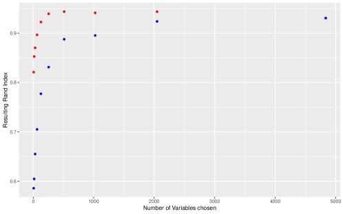
Figure 17: Rand index for the GISETTE data as a function of number of variables used. The red points correspond to ALB screening and blue points to $t$-statistic screening. Rand index is computed for a DART classifier using only those variables having the largest $2^{j}$ $t$-statistics or the largest $2^{j}$ values of $ALB$, where $j=3,\ldots,11$.

For these data, $t$-test screening does as well as ALB screening based on A4 and the 99.5th percentile. The difference between the two methods is that ALB retains the same accuracy while picking roughly 200 fewer variables. The interpretable cutoff rule does the worst, but 75% accuracy using only four “pixel” measurements is a very interesting result. We believe this is a setting where most variables, or ”pixels,” that are marginally important are ones that are colored in for one of the two numbers (4 or 9) but not the other. This can be interpreted as a location difference, since the intensity of a colored-in pixel is larger than the intensity of a pixel that is rarely touched. We also believe this is the reason why $t$-test screening finds more important variables than does ALB screening based on the same type I error rate. Despite being a setting where mostly location differences exist, ALB ends up doing as well as $t$-test screening in terms of Rand index, at least when using a type I error rate of $0.005$. In general we believe that choosing a cutoff based on a type I error rate or using 0 as a cutoff are good strategies for data sets where $n$ and $p$ are both large. A large amount of data allows us to choose fairly small significance thresholds while still maintaining good power. Choosing variables that have the largest $n+m$ values of ALB in this case results in no variables being screened, and so we elect not to explore that avenue. A cross-validation procedure for selecting a cutoff is expensive to perform due to the large values of $p$ and $n+m$.

To explore the impact of choosing a cutoff based on quantiles, we explored the Rand indices when the cutoff corresponded to using variables with the largest $k$ statistics. We considered values of $k$ that increased geometrically: $k=8,16,\ldots,2048$. The results can be seen in Figure 17. At each number of variables used, ALB-based screening has a larger Rand index than does $t$-test screening. Clearly, ALB and $t$-test screening are not choosing the same variables, and the ones chosen by ALB are more effective.

8 Application to Leukemia data

The Leukemia data set contains observations on 72 patients, 47 of which have one type of leukemia and the remainder another type. We have observations of 7129 variables on each patient to build a classifier that will help decide which type of leukemia a future patient has. This is a case where $p$ is much larger than $n$ and $m$. We will apply various screening methods to this problem in conjunction with DART and compare the accuracy of the methods via Rand indices.

To do this in a fair fashion, we split the data set randomly into two halves. The first half are validation data, and the second half are training data. We then split the training data in half again to make two smaller training sets. We do this for two reasons. First, we wish to assess the effect of training set size on accuracy of the methods. One of the two smaller training sets will be used to build classifiers, each one corresponding to a different screening method, and then all the training data will be used to build another set of classifiers. Both sets of classifiers will be used to predict the data in the validation set. The second reason for dividing the training set in half is that it makes possible a cross-validation approach for selecting a cutoff. We can train the model on one of the smaller training data sets, and choose a cutoff that gives the best classification accuracy on the other training data set. We can then train this best model on the full training set and apply it to the validation set. This is applying strategy A2 in the methodology, which is feasible because of the small sizes of $m$ and $n$.

To carry out our analysis we did the following. We performed four ALB based screening methods and two $t$-test based screening methods. The four ALB methods were A1 with the $n+m$ largest $ALB$s being selected, A2 with the cutoff of $0$, and A3 with a type I error rate of $0.05$, $d=3$ and $B=7129$.

Two methods of $t$-test screening were used, one using the variables with the $m+n$ largest $t$-statistics, and the other using variables whose $t$-test $P$-values were smaller than $0.05$. The latter version of $t$-test screening makes it comparable to choosing a variable using method A3 with significance level $0.05$. Once we determined relevant variables via screening, DART based on those variables was used to compute a Rand index from the validation set. Tables 2 and 3 summarize the results.

Rand Index	Screening Method Used	Number of variables
0.599	$n+m$ largest $ALB$s	19
0.529	$ALB>T^{*}_{0.05}$	617
0.599	$n+m$ largest $t$-statistics	19
0.529	$P_{t}<0.05$	847
0.501	No screening	7129

Table 2: Classification and screening results for leukemia data when training set is a quarter of full set. All results are based on a validation set size that was roughly half that of the full data set. The quantities $P_{t}$ and $T^{*}_{0.05}$ are, respectively, the $P$-value of a $t$-test and the 95th percentile of permuted $ALB$s. The classifier used was DART.

Rand Index	Screening Method	Number of variables
0.742	$ALB>T_{{\rm CV}}$	12
0.742	$ALB>T_{{\rm CV}}$	12
0.786	$n+m$ largest $ALB$s	38
0.572	$ALB>T^{*}_{0.05}$	1302
0.598	$n+m$ largest $t$-statistics	38
0.572	$P_{t}<.05$	1694
0.549	No screening	7129

Table 3: Classification and screening results for leukemia data when training set is half of full set. All results are based on a validation set size that was roughly half that of the full data set. The first two rows of the table correspond to use of the classifier based on (5), and subsequent rows to use of DART. The quantity $T_{CV}$ is the best cutoff as chosen by cross-validation, and $P_{t}$ and $T^{*}_{0.05}$ are as in Table 2. See Section 8 for an explanation of how cross-validation was implemented.

All screening methods performed similarly when the training set size was a quarter of $m+n$. However, $ALB$ screening that chose a cutoff as in $A1$ or $A3$ improved remarkably when the sample sizes were doubled, faring much better than the $t$-test based screening methods. While DART has been shown to be an effective classifier, our experience is that it may fail to recover the structure of the classification problem when the sample size is small. We thus tried the Bayesian classifier based on (5) with the CV-based method to choose a cutoff, and this classifier was able to achieve decent classification accuracy, surpassing DART if a different cutoff is chosen. We believe this is the case due to its simplicity, and there should be enough data to construct reasonable kernel density estimates of the underlying distributions.

Figure 18 shows the cross-validated Rand indices of the Bayesian classifier as a function of cutoff. It turns out that the largest cutoff maximizing the Rand index was .288. (The largest cutoff was chosen since this corresponds to the smallest number of variables maximizing the Rand index.) Figure 19 shows Rand indices of the Bayesian classifier that was trained on the full training set (i.e., the training set using half of the full data set). This figure shows how well the CV cutoff fared when it was used to screen variables in the full training set. Figure 18 shows how the number of variables chosen is related to cutoff. Finally, Figure 19 also shows how sensitive the Rand index is to the selected cutoff.

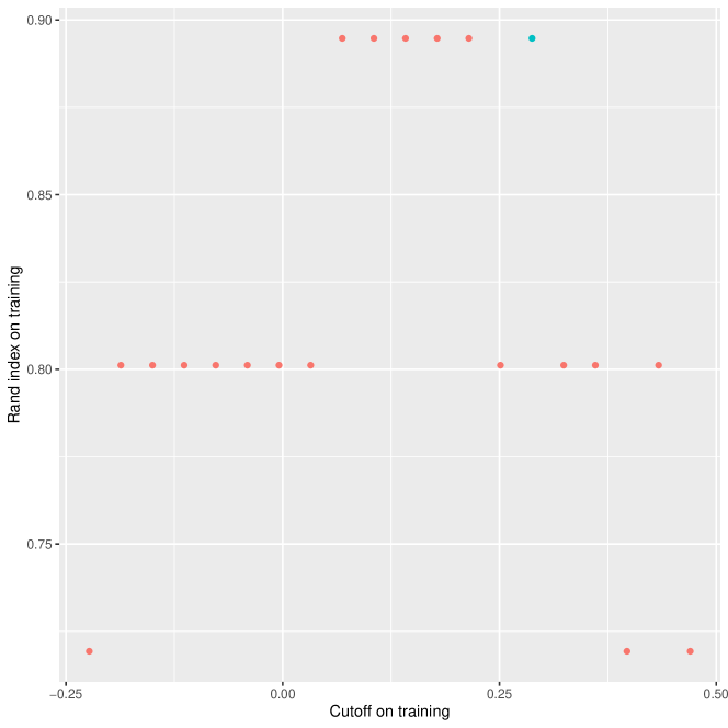
Figure 18: Cross-validation performance of the Bayesian classifier on the training set of the leukemia data. A plot of the Rand index of the method corresponding to (5) against the number of variables chosen by the method. The Rand indices are the performance of the classifier on one of the training sets, applied to the other training sets. We chose the cutoff that works best by picking the cutoff (in blue) that preserves the fewest variables in a sequence that maximizes the Rand index.

Figure 19: Cross-validation performance of the Bayesian classifier on the testing set of the leukemia data. The Rand indices are on the validation set. The cutoff we chose for cross validation is in blue ?? and was selected by examining Figure 18.

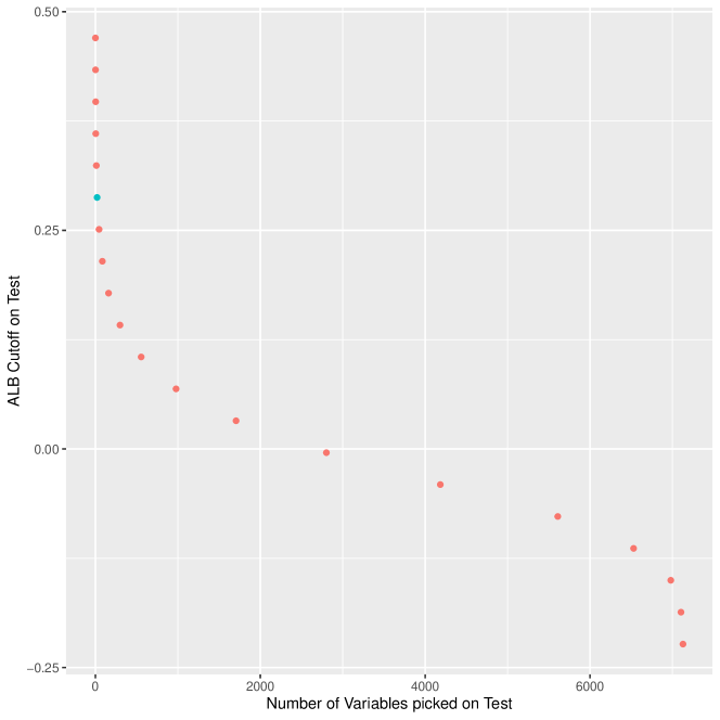
Figure 20: Number of variables picked versus the cutoff chosen using the ALB screening method on the Leukemia test data.

We believe the Bayesian classifier has potential in other settings where there may not be sufficient data to train ensemble methods and there may exist differences between classes that are not of location type. We note that, like other methods, it’s best to apply screening before using the Bayesian classifier, as all of their performances will degrade if there are a large amount of variables that are not useful. It is encouraging that the cutoff of $0$ was the largest cutoff before large improvements in Rand index occurred for the Bayesian classifier, but somewhat discouraging that the cross-validation approach could not pick a cutoff that resulted in the best performance for that classifier. The problem here is that the cross-validation approach chose an optimal cutoff when the classifier was constructed from one quarter of all the data, whereas we actually needed to know the optimal cutoff when half of all the data were used. Future research can focus on how an optimal cutoff depends on training set size. If the dependence is simple enough, it may be possible to estimate the optimal cutoff for a given training set size from cross-validation results based on a smaller training set size.

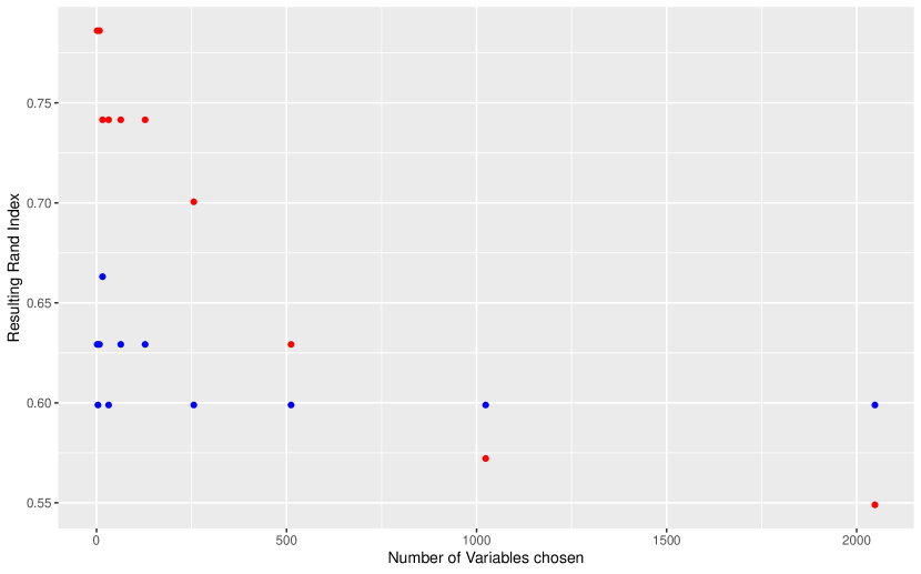
Figure 21: DART Rand indices versus number of variables chosen for the Leukemia data set. We plot the Rand index of the DART methods where we choose relevant variables corresponding to the top number of ALBs or $t$-statistics. We vary the number of variables chosen. The red points denote the Rand index of DART models using the top number of ALBs, while the blue points denote the Rand index of DART models using the top number of $t$-statistics.

ALB screening tends to do better when using the $k$ variables having the $k$ largest $ALB$s. Figure 21 shows the Rand index resulting from applying DART after using this method of screening. When using fewer than 500 variables, ALB screening does a better job than the analogous way of performing $t$-test screening. After the number of variables included is large enough, $t$-test screening does better than ALB screening, but at this point the number of variables included is large enough that the Rand index becomes suboptimal for both types of screening.

9 Conclusion and future work

We have proposed a new screening method that searches for differences other than those of location type. For this method to be more effective than $t$-test screening it needs to be paired with classification methods that can leverage these differences. In simulations, we pair ALB screening with BART, DART and a Bayesian classifier and show that it performs better than $t$-test screening in situations where class differences are not of location type. The Bayesian classier outperformed DART when applied to a leukemia data set. Even if the data contain primarily location differences, ALB screening performs well, although, as expected, not as well as $t$-test screening.

Future work includes efforts to increase the speed of computing ALB statistics and their permutation distributions, especially for large data sets. An iterative approach to the screening method is available for SIS, and future research could involve investigating an ALB procedure that could capture differences in joint distributions. The simulated data in this paper all leveraged independent data, and how sensitive the method is to independence is also a property to explore. The interaction between ALB screening and random projection or sketching methods of dealing with settings where $n$ and/or $p$ are very large is also a promising direction for future research.

References

- [Boser et al., 1992] Boser, B. E., Guyon, I. M., and Vapnik, V. N. (1992). A training algorithm for optimal margin classifiers. In Proceedings of the fifth annual workshop on Computational learning theory, pages 144–152.
- [Brieman et al., 1984] Brieman, L., Friedman, J. H., Olshen, R. A., and Stone, C. J. (1984). Classification and regression trees. Wadsworth Inc, 67.
- [Cui et al., 2015] Cui, H., Li, R., and Zhong, W. (2015). Model-free feature screening for ultrahigh dimensional discriminant analysis. Journal of the American Statistical Association, 110(510):630–641.
- [Fan and Lv, 2008] Fan, J. and Lv, J. (2008). Sure independence screening for ultrahigh dimensional feature space. Journal of the Royal Statistical Society: Series B (Statistical Methodology), 70(5):849–911.
- [Fan et al., 2010] Fan, J., Song, R., et al. (2010). Sure independence screening in generalized linear models with NP-dimensionality. The Annals of Statistics, 38(6):3567–3604.
- [Friedman, 2002] Friedman, J. H. (2002). Stochastic gradient boosting. Computational statistics & data analysis, 38(4):367–378.
- [Hill et al., 2020] Hill, J., Linero, A., and Murray, J. (2020). Bayesian Additive Regression Trees: A Review and Look Forward. Annual Review of Statistics and Its Application, 7.
- [Linero and Yang, 2018] Linero, A. R. and Yang, Y. (2018). Bayesian regression tree ensembles that adapt to smoothness and sparsity. Journal of the Royal Statistical Society: Series B (Statistical Methodology), 80(5):1087–1110.
- [Mai and Zou, 2012] Mai, Q. and Zou, H. (2012). The Kolmogorov filter for variable screening in high-dimensional binary classification. Biometrika, 100(1):229–234.
- [Merchant and Hart, 2022] Merchant, N. and Hart, J. (2022). A Bayesian motivated two-sample test based on kernel density estimates. Entropy, 24:1071.
- [Tang et al., 2014] Tang, J., Alelyani, S., and Liu, H. (2014). Feature selection for classification: A review. Data classification: Algorithms and applications, page 37.
- [Zhu et al., 2011] Zhu, L.-P., Li, L., Li, R., and Zhu, L.-X. (2011). Model-free feature screening for ultrahigh-dimensional data. Journal of the American Statistical Association, 106(496):1464–1475.