Strong pinning transition with arbitrary defect potentials

Abstract

Dissipation-free current transport in type II superconductors requires vortices, the topological defects of the superfluid, to be pinned by defects in the underlying material. The pinning capacity of a defect is quantified by the Labusch parameter $\kappa\sim f_{p}/\xi\bar{C}$, measuring the pinning force $f_{p}$ relative to the elasticity $\bar{C}$ of the vortex lattice, with $\xi$ denoting the coherence length (or vortex core size) of the superconductor. The critical value $\kappa=1$ separates weak from strong pinning, with a strong defect at $\kappa>1$ able to pin a vortex on its own. So far, this weak-to-strong pinning transition has been studied for isotropic defect potentials, resulting in a critical exponent $\mu=2$ for the onset of the strong pinning force density $F_{\mathrm{pin}}\sim n_{p}f_{p}(\xi/a_{0})^{2}(\kappa-1)^{\mu}$, with $n_{p}$ denoting the density of defects and $a_{0}$ the intervortex distance. This result is owed to the special rotational symmetry of the defect producing a finite trapping area $S_{\mathrm{trap}}\sim\xi^{2}$ at the strong-pinning onset. The behavior changes dramatically when studying anisotropic defects with no special symmetries: the strong pinning then originates out of isolated points with length scales growing as $\xi(\kappa-1)^{1/2}$, resulting in a different force exponent $\mu=5/2$. Our analysis of the strong pinning onset for arbitrary defect potentials $e_{p}(\mathbf{R})$, with $\mathbf{R}$ a planar coordinate, makes heavy use of the Hessian matrix describing its curvature and leads us to interesting geometrical structures: the strong pinning onset is characterized by the appearance of unstable areas of elliptical shape whose boundaries mark the locations where vortices jump. The associated locations of asymptotic vortex positions define areas of bistable vortex states; these bistable regions assume the shape of a crescent with boundaries that correspond to the spinodal lines in a thermodynamic first-order transition and cusps corresponding to critical end-points. Both, unstable and bistable areas grow with $\kappa>1$ and join up into larger domains; for a uniaxially anisotropic defect, two face to face crescents merge into the ring-shaped area previously encountered for the isotropic defect. Both, onset and merger points are defined by local differential properties of the Hessian’s determinant $D(\mathbf{R})$, specifically, its minima and saddle points. Extending our analysis to the case of a random two-dimensional pinning landscape, we discuss the topological properties of unstable and bistable regions as expressed through the Euler characteristic, with the latter related to the local differential properties of $D(\mathbf{R})$ through Morse theory.

I Introduction

Vortex pinning by material defects Campbell and Evetts (1972) determines the phenomenological properties of all technically relevant (type II) superconducting materials, e.g., their dissipation-free transport or magnetic response. Similar applies to the pinning of dislocations in metals Kassner (2015) or domain walls in magnets Gorchon et al. (2014), with the commonalities found in the topological defects of the ordered phase being pinned by defects in the host material: these topological defects are the vortices Abrikosov (1957), dislocations Burgers (1940), or domain walls Bloch (1932); Landau and Lifshitz (1935) appearing within the respective ordered phases—superconducting, crystalline, or magnetic. The theory describing the pinning of topological defects has been furthest developed in superconductors, with the strong pinning paradigm Labusch (1969); Larkin and Ovchinnikov (1979) having been strongly pushed during the last decade Blatter et al. (2004); Thomann et al. (2012); Willa et al. (2015); Buchacek et al. (2019a). In its simplest form, it boils down to the setup involving a single vortex subject to one defect and the cage potential Ertas and Nelson (1996); Vinokur et al. (1998) of other vortices. While still exhibiting a remarkable complexity, it produces quantitative results which benefit the comparison between theoretical predictions and experimental findings Buchacek et al. (2019b). So far, strong pinning has focused on isotropic defects, with the implicit expectation that more general potential shapes would produce small changes. This is not the case, as first demonstrated by Buchacek et al. Buchacek et al. (2020) in their study of correlation effects between defects that can be mapped to the problem of a string pinned to an anisotropic pinning potential. In the present work, we generalize strong pinning theory to defect potentials of arbitrary shape. We find that this simple generalization has pronounced (geometric) effects near the onset of strong pinning that even change the growth of the pinning force density $F_{\mathrm{pin}}\propto(\kappa-1)^{\mu}$ with increasing pinning strength $\kappa>1$ in a qualitative manner, changing the exponent $\mu$ from $\mu=2$ for isotropic defects Labusch (1969); Blatter et al. (2004) to $\mu=5/2$ for general anisotropic pinning potentials.

The pinning of topological defects poses a rather complex problem that has been attacked within two paradigms, weak-collective- and strong pinning. These have been developed in several stages: originating in the sixties of the last century, weak pinning and creep Larkin and Ovchinnikov (1979) has been further developed with the discovery of high temperature superconductors as a subfield of vortex matter physics Blatter et al. (1994). Strong pinning was originally introduced by Labusch Labusch (1969) and by Larkin and Ovchinnikov Larkin and Ovchinnikov (1979) and has been further developed recently with several works studying critical currents Blatter et al. (2004), current–voltage characteristics Thomann et al. (2012, 2017), magnetic field penetration Willa et al. (2015, 2016); Gaggioli et al. (2022), and creep Buchacek et al. (2018, 2019a); Gaggioli et al. (2022); results on numerical simulations involving strong pins have been reported in Refs. Kwok et al., 2016; Willa et al., 2018a, b. The two theories come together at the onset of strong pinning: an individual defect is qualified as weak if it is unable to pin a vortex, i.e., a vortex traverses the pin smoothly. Crossing a strong pin, however, the vortex undergoes jumps that mathematically originate in bistable distinct vortex configurations, ‘free’ and ‘pinned’. Quantitatively, the onset of strong pinning is given by the Labusch criterion $\kappa=1$, with the Labusch parameter $\kappa\equiv\max[-e_{p}^{\prime\prime}]/\bar{C}\sim f_{p}/\xi\bar{C}$, the dimensionless ratio of the negative curvature $e_{p}^{\prime\prime}$ of the isotropic pinning potential and the effective elasticity $\bar{C}$ of the vortex lattice. Strong pinning appears for $\kappa>1$, i.e., when the lattice is soft compared to the curvatures in the pinning landscape.

So far, the strong pinning transition at $\kappa=1$ has been described for defects with isotropic pinning potentials; it can be mapped Blatter et al. (2004) to the magnetic transition in the $h$-$T$ (field–temperature) space, with the strong-pinning phenomenology at $\kappa>1$ corresponding to the first-order Ising magnetic transition at $T<T_{c}$ and the critical point at $T=T_{c}$ corresponding to the strong pinning transition at $\kappa=1$. The role of the reduced temperature $T/T_{c}$ is then assumed by the Labusch parameter $\kappa$ and the bistabilities associated with the ferromagnetic phases at $T/T_{c}<1$ translate to the bistable pinned and free vortex states at $\kappa>1$, with the bistability disappearing on approaching the critical point, $T/T_{c}=1$ and $\kappa=1$, respectively.

A first attempt to account for correlations between defects has been done in Ref. Buchacek et al., 2020. The latter analysis takes into account the enhanced pinning force excerted by pairs of isotropic defects that can be cast in the form of anisotropic effective pinning centers. Besides shifting the onset of strong pinning to $\kappa=1/2$ (with $\kappa$ defined for one individual defect), the analysis unravelled quite astonishing (geometric) features that appeared as a consequence of the symmetry reduction in the pinning potential. In the present paper, we take a step back and study the transition to strong pinning for anisotropic defect potentials $e_{p}({\bf R})$, with $\mathbf{R}$ a planar coordinate, see Fig. 1. Note that collective effects of many weak defects can add up to effectively strong pins that smoothen the transition at $\kappa=1$, thereby turning the strong pinning transition into a weak-to-strong pinning crossover.

We find that the onset of strong pinning proceeds quite differently when going from the isotropic defect to the anisotropic potential of a generic defect without special symmetries and further on to a general random pinning landscape. The simplest comparison is between an isotropic and a uniaxially anisotropic defect, acting on a vortex lattice that is directed along the magnetic field ${\bf B}\parallel{\bf e}_{z}$ chosen parallel to the $z$-axis; for convenience, we place the defect at the origin of our coordinate system ${\bf r}=({\bf R},z)$ and have it act only in the $z=0$-plane. In this setup, see Fig. 1, the pinning potential $e_{p}({\bf R})$ acts on the nearest vortex with a force ${\bf f}_{p}({\bf R})=-\nabla_{\bf R}e_{p}|_{z=0}$ attracting the vortex to the defect; the presence of the other vortices constituting the lattice renormalizes the vortex elasticity $\bar{C}$. With the pinning potential acting in the $z=0$ plane, the vortex is deformed with a pronounced cusp at $z=0$, see Fig. 1; we denote the tip position of the vortex where the cusp appears by $\tilde{\bf R}$, while the asymptotic position of the vortex at $z\to\pm\infty$ is fixed at $\bar{\bf R}$. With this setup the problem can be reduced to a planar one, with the tip coordinate $\tilde{\bf R}$ and the asymptotic coordinate $\bar{\bf R}$ determining the location and full shape (and hence the pinning force) of the vortex line.

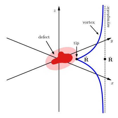
Figure 1: Sketch of a vortex interacting with a defect located at the origin. The vortex approaches the asymptotic position $\bar{\bf R}$ at $z\to\pm\infty$ and is attracted to the defect residing at the origin; the cusp at $z=0$ defines the tip position $\tilde{\bf R}$ and its angle quantifies the pinning strength.

In the case of an isotropic pin, e.g., produced by a point-like defect Thomann et al. (2012), strong pinning first appears on a circle of finite radius $R_{m}\sim\xi$, typically of order of the vortex core radius $\xi$, see left panel of Fig. 2(a). This is owed to the fact that, given the radial symmetry, the Labusch criterion $\kappa=\max_{R}[-e_{p}^{\prime\prime}(R)]/\bar{C}=1$ is satisfied on a circle $R=R_{m}$ where the (negative) curvature $-e_{p}^{\prime\prime}>0$ is maximal. Associated with the radius $R_{m}$ where the tip is located at $\kappa=1$, $\tilde{R}(\kappa=1)\equiv\tilde{R}_{m}=R_{m}$, there is an asymptotic vortex position $\bar{R}(\kappa=1)=\bar{R}_{m}>\tilde{R}_{m}$. Increasing the Labusch parameter beyond $\kappa=1$, the circle of radius $\bar{R}_{m}$ transforms into a ring $\bar{R}_{-}<\bar{R}<\bar{R}_{+}$ of finite width. Vortices placed inside the ring at small distances $\bar{R}<\bar{R}_{-}$ near the defect are qualified as ‘pinned’, while vortices at large distances $\bar{R}>\bar{R}_{+}$ away from the pin are described as ‘free’, see right panel in Fig. 2(a); physically, we denote a vortex configuration as ‘free’ when it is smoothly connected to the asymptotic undeformed state, while a ‘pinned’ vortex is localized to a finite region around the defect. Vortices placed inside the bistable ring at $\bar{R}_{-}<\bar{R}<\bar{R}_{+}$ acquire two possible states, pinned and free (colored magenta in Fig. 2, the superposition of red (pinned state) and blue (free state) colors).

The onset of strong pinning for the uniaxially anisotropic defect proceeds in several stages. Let us consider an illustrative example and assume a defect with an anisotropy aligned with the axes and a steeper potential along $x$. In this situation, strong pinning as defined by the criterion $\kappa_{m}=1$, with a properly generalized Labusch parameter $\kappa_{m}$, appears out of two points $(\pm\bar{x}_{m},0)$ where the Labusch criterion $\kappa_{m}=1$ is met first, see Fig. 2(b) left. Increasing $\kappa_{m}>1$ beyond unity, two bistable domains spread around these points and develop two crescent-shaped areas (with their large extent along $\bar{y}$) in asymptotic $\bar{\bf R}$-space, see Fig. 2(b) right. Vortices with asymptotic positions within these crescent-shaped regions experience bistability, while outside these regions the vortex state is unique. Classifying the bistable solutions as ‘free’ and ‘pinned’ is not possible, with the situation resembling the one around the gas–liquid critical point with a smooth crossover (from blue to white to red) between phases. With $\kappa_{m}$ increasing further, the cusps of the crescents approach one another. As the arms of the two crescents touch and merge at a sufficiently large value of $\kappa_{m}$, the topology of the bistable area changes: the two merged crescents now define a ring-like geometry and separate $\bar{\bf R}$-space into an inside region where vortices are pinned, an outside region where vortices are free and the bistable region with pinned and free states inside the ring-like region. As a result, the pinning geometry of the isotropic defect is recovered, though with the perfect ring replaced by a deformed ring with varying width. Using the language describing a thermodynamic first-order transition, the cusps of the crescents correspond to critical points while its boundaries map to spinodal lines; the merging of critical points changing the topology of the bistable regions of the pinning landscape goes beyond the standard thermodynamic analogue of phase diagrams.

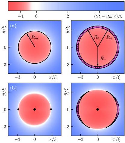
Figure 2: Illustration of bistable regions in asymptotic $\bar{\bf R}$-space for a vortex pinned to a defect located at the origin. (a) For an isotropic defect (Lorentzian shape with $\kappa=1,~{}1.5$), pinning appears at $\kappa=1$ along a ring with radius $\bar{R}_{m}$, with the red area corresponding to pinned states and free states colored in blue. With increasing pinning strength $\kappa$, see right panel at $\kappa=1.5$, a bistable region (in magenta) appears in a ring geometry, with vortices residing inside, $\bar{R}<\bar{R}_{-}$, being pinned and vortices outside, $\bar{R}>\bar{R}_{+}$, remaining free. Vortices with asymptotic positions inside the ring ($\bar{R}_{-}<\bar{R}<\bar{R}_{+}$) exhibit bistable states, pinned and free. The dashed circle $\bar{R}_{0}$ marks the crossing of pinned and free branches, see Fig. 4. (b) For a uniaxially anisotropic defect, see Eq. (94) with $\epsilon=0.3$ and largest (negative) curvature along $x$, pinning appears in two points $(\pm\bar{x}_{m},0)$ along the $x$-axis. As the pinning strength increases beyond unity, see right panel, bistable regions (magenta) develop in a crescent-shape geometry. Pinned- and free-like states are smoothly connected as indicated by the crossover of colors (see Sec. III.3 for the precise description of coloring in terms of an ‘order parameter’). As $\kappa_{m}$ further increases, the cusps of the two crescents merge on the $y$-axis, changing the topology of the $\bar{\bf R}$-plane through separation into inner and outer regions (not shown). A ring-like bistable region appears as in $(\mathrm{a})$, with the inner (outer) region corresponding to unique vortex states that are pinned (free), while vortices residing inside the ring-shaped domain exhibit bistable states, pinned and free.

The bistable area is defining the trapping area where vortices get pinned to the defect; this trapping area is one of the relevant quantities determining the pinning force density $F_{\mathrm{pin}}$, the other being the jumps in energy associated with the difference between the bistable states Labusch (1969); Blatter et al. (2004), see the discussion in Secs. II.3, II.5, and III.7 below. It is the change in the bistable- and hence trapping geometry that modifies the exponent $\mu$ in $F_{\mathrm{pin}}\propto(\kappa-1)^{\mu}$, replacing the exponent $\mu=2$ for isotropic defects by the new exponent $\mu=5/2$ for general anisotropic pinning potentials.

While the existence of bistable regions $\mathcal{B}_{\bar{\bf R}}$ in the space of asymptotic vortex positions $\bar{\bf R}$ is an established element of strong pinning theory by now, in the present paper, we introduce the new concept of unstable domains $\mathcal{U}_{\tilde{\bf R}}$ in tip-space. The two coordinates $\tilde{\bf R}$ and $\bar{\bf R}$ represent dual variables in the sense of the thermodynamic analog, with the asymptotic coordinate $\bar{\bf R}$ corresponding to the driving field $h$ in the Ising model and the tip position $\tilde{\bf R}$ replacing the magnetic response $m$; from a thermodynamic perspective it is then quite natural to change view by going back and forth between intensive ($h$) and extensive ($m$) variables. In tip space $\tilde{\bf R}$, the onset of pinning appears at isolated points $\tilde{\bf R}_{m}$ that grow into ellipses as $\kappa$ is increased beyond unity. These ellipses describe unstable areas $\mathcal{U}_{\tilde{\bf R}}$ in the $\tilde{\bf R}$-plane across which vortex tips jump when flipping between bistable states; they relate to the bistable crescent-shaped areas $\mathcal{B}_{\bar{\bf R}}$ in asymptotic space through the force balance equation; the latter determines the vortex shape with elastic and pinning forces compensating one another. The unstable regions $\mathcal{U}_{\tilde{\bf R}}$ in tip space are actually more directly accessible than the bistable regions $\mathcal{B}_{\bar{\bf R}}$ in asymptotic space and play an equally central role in the discussion of the strong pinning landscape.

The simplification introduced by the concept of unstable domains $\mathcal{U}_{\tilde{\bf R}}$ in tip space $\tilde{\bf R}$ is particularly evident when going from individual defects as described above to a generic pinning landscape. Here, we focus on a model pinning potential landscape (or short pinscape) confined to the two-dimensional (2D) $\mathbf{R}$ plane at $z=0$; such a pinscape can be produced, e.g., by defects that reside in the $z=0$ plane. The pinned vortex tip $\tilde{\bf R}$ then still resides in the $z=0$ plane as well and the strong pinning problem remains two-dimensional. For a 2D random pinscape, unstable ellipses appear sequentially out of different (isolated) points and at different pinning strength $\kappa_{m}$; their assembly defines the unstable area $\mathcal{U}_{\tilde{\bf R}}$, with each newly appearing ellipse changing the topology of $\mathcal{U}_{\tilde{\bf R}}$, specifically, its number of components. Increasing $\kappa_{m}$, the ellipses first grow in size, then deform away from their original elliptical shapes, and finally touch and merge in a hyperbolic geometry. Such mergers change, or more precisely reduce, the number of components in $\mathcal{U}_{\tilde{\bf R}}$ and hence correspond again to topological transitions as described by a change in the Euler characteristic $\chi$ associated with the shape of $\mathcal{U}_{\tilde{\bf R}}$. Furthermore, these mergers tend to produce $\mathcal{U}_{\tilde{\bf R}}$ shapes that are non-simply connected, again implying a topological transition in $\mathcal{U}_{\tilde{\bf R}}$ with a change in $\chi$. Such non-simply connected parts of $\mathcal{U}_{\tilde{\bf R}}$ separate the tip space into ‘inner’ and ‘outer’ regions that allows to define proper ‘pinned’ states (localized near a potential minimum) in the ‘inner’ of $\mathcal{U}_{\tilde{\bf R}}$, while ‘free’ states (smoothly connected to asymptotically undeformed vortices) occupy the regions outside of $\mathcal{U}_{\tilde{\bf R}}$.

The discussion below is dominated by three mathematical tools: for one, it is the Hessian matrix $\mathrm{H}({\bf R})$ of the pinning potential Buchacek et al. (2020); Willa et al. (2022) $e_{p}({\bf R})$, its eigenvalues $\lambda_{\pm}({\bf R})$ and eigenvectors ${\bf v}_{\pm}({\bf R})$, its determinant $\det[\mathrm{H}]({\bf R})$ and trace $\tr[\mathrm{H}]({\bf R})$. The Hessian matrix involves the curvatures $\mathrm{H}_{ij}=\partial_{i}\partial_{j}e_{p}({\bf R})$, $i,j\in\{x,y\}$, of the pinning potential, that in turn are the quantities determining strong pinning, as can be easily conjectured from the form of the Labusch parameter $\kappa\propto-e_{p}^{\prime\prime}$ for the isotropic defect. The second tool is the Landau-type expansion of the total pinning energy near the strong-pinning onset around $\tilde{\bf R}_{m}$ at $\kappa_{m}=1$ (appearance of a critical point) as well as near merging around $\tilde{\bf R}_{s}$ at $\kappa(\tilde{\bf R}_{s})\equiv\kappa_{s}=1$ (disappearance of a pair of critical points); the standard manipulations as they are known from the description of a thermodynamic first-order phase transition produce most of the new results. Third, the topological structure of the unstable domain $\mathcal{U}_{\tilde{\bf R}}$ associated with a generic 2D pinning landscape, i.e., its components and their connectedness, is conveniently described through its Euler characteristic $\chi$ with the help of Morse theory.

The structure of the paper is as follows: In Section II, we briefly introduce the concepts of strong pinning theory with a focus on the isotropic defect. The onset of strong pinning by a defect of arbitrary shape is presented in Sec. III; we start with a translation and extension of the strong pinning ideas from the isotropic situation to a general anisotropic one, that leads us to the Hessian analysis of the pinning potential as our basic mathematical tool. Close to onset, we find (using a Landau-type expansion, see Sec. III.1) that the unstable (Sec. III.2) and bistable (Sec. III.3) domains are associated with minima of the determinant of the Hessian curvature matrix and assume the shape of an ellipse and a crescent, respectively. Due to the anisotropy, the geometry of the trapping region depends non-trivially on the Labusch parameter and the critical exponent for the pinning force is changed from $\mu=2$ to $\mu=5/2$, see Sec. III.7. The analytic solution of the strong pinning onset for a weakly uniaxial defect presented in Sec. IV leads us to define new hyperbolic points associated with saddle points of the determinant of the Hessian curvature matrix. These hyperbolic points describe the merging of unstable and bistable domains, see Sec. V.1, and allow us to relate the new results for the anisotropic defect to our established understanding of isotropic defects. In a final step, we extend the local perspective on the pinscape, as acquired through the analysis of minima and saddles of the determinant of the Hessian curvature matrix, to a global description in terms of the topological characteristics of the unstable domain $\mathcal{U}_{\tilde{\bf R}}$: in Sec. VI, we discuss strong pinning in a two-dimensional pinning potential of arbitrary shape, e.g., as it appears when multiple pinning defects overlap (though all located in one plane). We follow the evolution of the unstable domain $\mathcal{U}_{\tilde{\bf R}}$ with increasing pinning strength $\kappa_{m}$ and express its topological properties through the Euler characteristic $\chi$; the latter is related to the local differential properties of the pinscape’s curvature, its minima, saddles, and maxima, through Morse theory. Finally, in Appendix A, we map the two-dimensional Landau-type theories (involving two order parameters) describing onset and merging, to effective one-dimensional Landau theories and rederive previous results following standard statistical mechanics calculations as they are performed in the analysis of the critical point in the van der Waals gas.

II Strong pinning theory

We start with a brief introduction to strong pinning theory, keeping a focus on the transition region at moderate values of $\kappa>1$. We consider an isotropic defect (Sec. II.1) and determine the unstable and bistable ring domains for this situation in Sec. II.2. We derive the general expression for the pinning force density $F_{\mathrm{pin}}$ in Sec. II.3, determine the relevant scales of the strong pinning characteristic near the crossover in Sec. II.4, and apply the results to derive the scaling $F_{\mathrm{pin}}\propto(\kappa-1)^{2}$ for the isotropic defect (Sec. II.5). In Sec. II.6, we relate the strong pinning theory for the isotropic defect to the Landau mean-field description for the Ising model in a magnetic field.

II.1 Isotropic defect

The standard strong-pinning setup involves a vortex lattice directed along $z$ with a lattice constant $a_{0}$ determined by the induction $B=\phi_{0}/a_{0}^{2}$ that is interacting with a dilute set of randomly arranged defects of density $n_{p}$. This many-body problem can be reduced Blatter et al. (2004); Willa et al. (2016); Buchacek et al. (2019a) to a much simpler effective problem involving an elastic string with effective elasticity $\bar{C}$ that is pinned by a defect potential $e_{p}({\bf R})$ acting in the origin, as described by the energy function

$$e_{\mathrm{pin}}(\tilde{\bf R};\bar{\bf R})=\frac{\bar{C}}{2}(\tilde{\bf R}-\bar{\bf R})^{2}+e_{p}(\tilde{\bf R})$$ (1)

depending on the tip- and asymptotic coordinates $\tilde{\bf R}$ and $\bar{\bf R}$ of the vortex, see Fig. 1. The energy (or Hamiltonian) $e_{\mathrm{pin}}(\tilde{\bf R};\bar{\bf R})$ of this setup involves an elastic term and the pinning energy $e_{p}({\bf R})$ evaluated at the location $\tilde{\bf R}$ of the vortex tip. We denote the depth of the pinning potential by $e_{p}$. A specific example is the point-like defect that produces an isotropic pinning potential which is determined by the form of the vortex Thomann et al. (2012) and assumes a Lorentzian shape $e_{p}(R)=-e_{p}/(1+R^{2}/2\xi^{2})$ with $R=\absolutevalue{{\bf R}}$; in Sec. III below, we will consider pinning potentials of arbitrary shape $e_{p}({\bf R})$ but assume a small (compared to the coherence length $\xi$) extension along $z$. ‘Integrating out’ the vortex lattice, the remaining string or vortex is described by the effective elasticity $\bar{C}\approx\nu\varepsilon(a_{0}^{2}/\lambda_{\rm\scriptscriptstyle L})\sqrt{c_{66}c_{44}(0)}\sim\varepsilon\varepsilon_{0}/a_{0}$. Here, $\varepsilon_{0}=(\phi_{0}/4\pi\lambda_{\rm\scriptscriptstyle L})^{2}$ is the vortex line energy, $\lambda_{\rm\scriptscriptstyle L}$ denotes the London penetration depth, $\varepsilon<1$ is the anisotropy parameter for a uniaxial material Blatter et al. (1994), and $\nu$ is a numerical, see Refs. Kwok et al., 2016; Willa et al., 2018b.

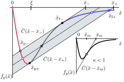
Figure 3: Graphical illustrationBuchacek et al. (2019a) of the self-consistent solution of the microscopic force-balance equation Eq. (2) for a Lorentzian potential with $\kappa=2.5$. The vortex coordinates $\tilde{x}$ and $\bar{x}$ are expressed in units of $\xi$. When moving the asymptotic vortex position $\bar{x}$ across the bistable interval $[\bar{x}_{-},\bar{x}_{+}]$, we obtain three solutions describing pinned $\tilde{x}_{\mathrm{p}}\lesssim\xi$, free $\tilde{x}_{\mathrm{f}}$ close to $\bar{x}$, and unstable $\tilde{x}_{\mathrm{us}}$ states; they define the corresponding pinned (red), free (blue), and unstable (black dotted) branches. The tip-positions at the edges of the bistable interval denoted by $\tilde{x}_{\mathrm{p+}}$ and $\tilde{x}_{\mathrm{f-}}$ denote jump points where the vortex tip turns unstable, see Eq. (3); they are defined by the condition $f^{\prime}_{p}(\tilde{x}_{\mathrm{p+}})=f^{\prime}_{p}(\tilde{x}_{\mathrm{f-}})=\bar{C}$ (black solid dots). The associated positions $\tilde{x}_{\mathrm{f+}}$ and $\tilde{x}_{\mathrm{p-}}$ denote the tip landing points after the jump (open circles); they are given by the second solution of Eq. (2) at the same asymptotic position $\bar{x}$. The open red/blue circles and the cross mark the positions of metastable minima and the unstable maximum in Fig. 4. The lower right inset shows the weak-pinning situation at $\kappa<1$, here implemented with a larger $\bar{C}$, where the tip solution $\tilde{x}$ is unique for all $\bar{x}$.

The most simple pinning geometry is for a vortex that traverses the defect through its center. Given the rotational symmetry of the isotropic defect, we choose a vortex that impacts the defect in a head-on collision from the left with asymptotic coordinate $\bar{\bf R}=(\bar{x},0)$ and increase $\bar{x}$ along the $x$-axis; finite impact parameters $\bar{y}\neq 0$ will be discussed later. The geometry then simplifies considerably and involves the asymptotic vortex position $\bar{x}$ and the tip position $\tilde{x}$ of the vortex, reducing the problem to a one-dimensional one; the full geometry of the deformed string can be determined straightforwardly Willa et al. (2016) once the tip position $\tilde{x}$ has been found. The latter follows from minimizing (1) with respect to $\tilde{x}$ at fixed asymptotic position $\bar{x}$ and leads to the non-linear equation

$$\bar{C}(\tilde{x}-\bar{x})=-\partial_{x}e_{p}|_{x=\tilde{x}}=f_{p}(\tilde{x}).$$ (2)

This can be solved graphically, see Fig. 3, and produces either a single solution or multiple solutions—the appearance of multiple tip solutions is the signature of strong pinning. The relevant parameter that distinguishes the two cases is found by taking the derivative of (2) with respect to $\bar{x}$ that leads to

$$\partial_{\bar{x}}\tilde{x}=\frac{1}{1-f_{p}^{\prime}(\tilde{x})/\bar{C}},$$ (3)

where prime denotes the derivative, $f^{\prime}_{p}(x)=\partial_{x}f_{p}(x)=-\partial_{x}^{2}e_{p}(x)$. Strong pinning involves vortex instabilities, i.e., jumps in the tip coordinate $\tilde{x}$, that appear when the denominator in (3) vanishes; this leads us to the strong pinning parameter $\kappa$ first introduced by Labusch Labusch (1969),

$$\kappa=\max_{\tilde{x}}\frac{f^{\prime}_{p}(\tilde{x})}{\bar{C}}=\frac{f^{\prime}_{p}(\tilde{x}_{m})}{\bar{C}},$$ (4)

with $\tilde{x}_{m}$ defined as the position of maximal force derivative $f_{p}^{\prime}$, i.e., $f_{p}^{\prime\prime}(\tilde{x}_{m})=0$, or maximal negative curvature $-e_{p}^{\prime\prime}$ of the defect potential. Defining the force scale $f_{p}\equiv e_{p}/\xi$ and estimating the force derivative or curvature $f_{p}^{\prime}=-e_{p}^{\prime\prime}\sim f_{p}/\xi$ produces a Labusch parameter $\kappa\sim e_{p}/\bar{C}\xi^{2}$; for the Lorentzian potential, we find that $f_{p}^{\prime}(\tilde{x}_{m})=e_{p}/4\xi^{2}$ at $\tilde{x}_{m}=\sqrt{2}\,\xi$ and hence $\kappa=e_{p}/4\bar{C}\xi^{2}$. We see that strong pinning is realized for either large pinning energy $e_{p}$ or small effective elasticity $\bar{C}$.

As follows from Fig. 3 (inset), for $\kappa<1$ (large $\bar{C}$) the solution to Eq. (2) is unique for all values of $\bar{x}$ and pinning is weak, while for $\kappa>1$ (small $\bar{C}$), multiple solutions appear in the vicinity of $\tilde{x}_{m}$ and pinning is strong. These multiple solutions appear in a finite interval $\bar{x}\in[\bar{x}_{-},\bar{x}_{+}]$ and we denote them by $\tilde{x}=\tilde{x}_{\mathrm{f}},\tilde{x}_{\mathrm{p}},\tilde{x}_{\mathrm{us}}$, see Fig. 3; they are associated with free (weakly deformed vortex with $\tilde{x}_{\mathrm{f}}$ close to $\bar{x}$), pinned (strongly deformed vortex with $\tilde{x}_{\mathrm{p}}<\xi$), and unstable vortex states.

Inserting the solutions $\tilde{x}(\bar{x})=\tilde{x}_{\mathrm{f}}(\bar{x}),\tilde{x}_{\mathrm{p}}(\bar{x}),\tilde{x}_{\mathrm{us}}(\bar{x})$ of Eq. (2) at a given vortex position $\bar{x}$ back into the pinning energy $e_{\mathrm{pin}}(\tilde{x};\bar{x})$, we find the energies of the corresponding branches,

$$e^{\mathrm{i}}_{\mathrm{pin}}(\bar{x})\equiv e_{\mathrm{pin}}[\tilde{x}_{\mathrm{i}}(\bar{x});\bar{x}],\quad\mathrm{i}=\mathrm{f,p,us}.$$ (5)

The pair $e_{p}(\tilde{x})$ and $e^{\mathrm{i}}_{\mathrm{pin}}(\bar{x})$ of energies in tip- and asymptotic spaces then has its correspondence in the force: associated with $f_{p}(\tilde{x})$ in tip space are the force branches $f^{\mathrm{i}}_{\mathrm{pin}}(\bar{x})$ in asymptotic $\bar{x}$-space defined as

$$f^{\mathrm{i}}_{\mathrm{pin}}(\bar{x})=f_{p}[\tilde{x}_{\mathrm{i}}(\bar{x})],\quad\textrm{i}=\mathrm{f,p,us}.$$ (6)

Using Eq. (2), it turns out that the force $f_{\mathrm{pin}}$ can be written as the total derivative of $e_{\mathrm{pin}}$,

$$f_{\mathrm{pin}}(\bar{x})=-\frac{de_{\mathrm{pin}}[\tilde{x}(\bar{x});\bar{x}]}{d\bar{x}}.$$ (7)

The multiple branches $e^{\mathrm{i}}_{\mathrm{pin}}$ and $f^{\mathrm{i}}_{\mathrm{pin}}$ associated with a strong pinning situation at $\kappa>1$ are shown in Figs. 4 and 5$(\mathrm{b})$.

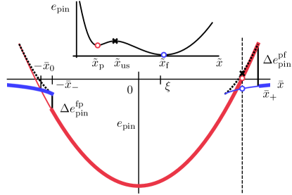
Figure 4: Multi-valued pinning energy landscape $e_{\mathrm{pin}}^{\mathrm{i}}(\bar{x})$ for a defect producing a Lorentzian-shaped potential with $\kappa=2.5$; the branches $\mathrm{i}=\mathrm{p,f,us}$ correspond to the pinned (red), free (blue), and unstable (black dotted) vortex states. The bistability extends over the intervals $|\bar{x}|\in\left[\bar{x}_{-},\bar{x}_{+}\right]$ where the different branches coexist; pinned and free vortex branches cut at the branch crossing point $\bar{x}=\bar{x}_{0}$. A vortex traversing the defect from left to right assumes the free and pinned states marked with thick colored lines and undergoes jumps $\Delta e_{\mathrm{pin}}^{\mathrm{fp}}$ and $\Delta e_{\mathrm{pin}}^{\mathrm{pf}}$ in energy (vertical black solid lines) at the boundaries $-\bar{x}_{-}$ and $\bar{x}_{+}$. The asymmetric occupation of states produces a finite pinning force density $F_{\mathrm{pin}}$. Inset: Total energy $e_{\mathrm{pin}}(\tilde{x};\bar{x})$ versus vortex tip position $\tilde{x}$ for a fixed vortex position $\bar{x}$ (vertical dashed line in the main figure). The points $\tilde{x}_{\mathrm{f}}$, $\tilde{x}_{\mathrm{p}}$, and $\tilde{x}_{\mathrm{us}}$ mark the free, pinned, and unstable solutions of the force-balance equation (2); they correspond to local minima and the maximum in $e_{\mathrm{pin}}(\tilde{x};\bar{x})$ and are marked with corresponding symbols in Fig. 3.

II.2 Unstable and bistable domains $\mathcal{U}_{\tilde{\bf R}}$ and $\mathcal{B}_{\bar{\bf R}}$

Next, we identify the unstable (in $\tilde{x}$) and bistable (in $\bar{x}$) domains of the pinning landscape that appear as signatures of strong pinning when $\kappa$ increases beyond unity. Figure 5(a) shows the force profile $f_{p}(\tilde{x})$ as experienced by the tip coordinate $\tilde{x}$. A vortex passing the defect on a head-on trajectory from left to right undergoes a forward jump in the tip from $-\tilde{x}_{\mathrm{f-}}$ to $-\tilde{x}_{\mathrm{p-}}$; subsequently, the tip follows the pinned branch until $\tilde{x}_{\mathrm{p+}}$ and then returns back to the free state with a forward jump from $\tilde{x}_{\mathrm{p+}}$ to $\tilde{x}_{\mathrm{f+}}$. The jump positions (later indexed by a subscript ‘$\mathrm{jp}$’) are determined by the two solutions of the equation

$$f_{p}^{\prime}(x)\Big{|}_{-\tilde{x}_{\mathrm{f-}},\tilde{x}_{\mathrm{p+}}}=\bar{C}$$ (8)

that involves the curvature of the pinning potential $e_{p}(x)$; the landing positions $-\tilde{x}_{\mathrm{p-}}$ and $\tilde{x}_{\mathrm{f+}}$ (later indexed by a subscript ‘$\mathrm{lp}$’), on the other hand, are given by the second solution of the force-balance equation (2) that involves the driving term $\bar{C}(\tilde{x}-\bar{x})$ and hence depends on the asymptotic position $\bar{x}$. Finally, the positions in asymptotic space $\bar{x}$ where the vortex tip jumps are obtained again from the force balance equation (2),

$$\bar{x}_{-} = \tilde{x}_{\mathrm{f-}}-f_{p}(\tilde{x}_{\mathrm{f-}})/\bar{C},$$ (9)

$$\bar{x}_{+} = \tilde{x}_{\mathrm{p+}}-f_{p}(\tilde{x}_{\mathrm{p+}})/\bar{C}.$$

Note that the two pairs of tip jump and landing positions, $\tilde{x}_{\mathrm{p+}},~{}\tilde{x}_{\mathrm{f+}}$ and $\tilde{x}_{\mathrm{f-}},~{}\tilde{x}_{\mathrm{p-}}$ are associated with only two asymptotic positions $\bar{x}_{+}$ and $\bar{x}_{-}$.

Let us generalize the geometry and consider a vortex moving parallel to $\bar{x}$, impacting the defect at a finite distance $\bar{y}$. We then have to extend the above discussion to the entire $z=0$ plane, see Fig. 5. For an isotropic defect, the jump- and landing points now define jump circles with radii $\tilde{R}_{\mathrm{jp}}$ given by $\tilde{R}_{\mathrm{f-}}=\tilde{x}_{\mathrm{f-}}$ and $\tilde{R}_{\mathrm{p+}}=\tilde{x}_{\mathrm{p+}}$ (solid circles in Fig. 5$(\mathrm{c})$) and landing circles with radii $\tilde{R}_{\mathrm{lp}}$ given by $\tilde{R}_{\mathrm{f+}}=\tilde{x}_{\mathrm{f+}}$, $\tilde{R}_{\mathrm{p-}}=\tilde{x}_{\mathrm{p-}}$ (dashed circles in Fig. 5$(\mathrm{c})$). Their combination defines an unstable ring $\tilde{R}_{\mathrm{p+}}<\tilde{R}<\tilde{R}_{\mathrm{f-}}$ in tip space where tips cannot reside. The existence of unstable domains $\mathcal{U}_{\tilde{\bf R}}$ in tip space is a signature of strong pinning.

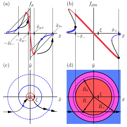
Figure 5: (a) and (b): Force profiles $f_{p}(\tilde{x})$ and $f_{\mathrm{pin}}(\bar{x})$ in tip- and asymptotic coordinates for a Lorentzian-shaped potential with $\kappa=2.5$. The tip of a vortex moving from left to right along the $x$-axis approaches the defect on the free branch (thick blue line) undergoes a jump (arrow) from $-\tilde{x}_{\mathrm{f-}}$ to $-\tilde{x}_{\mathrm{p-}}$, follows the pinned branch (red) until $\tilde{x}_{\mathrm{p+}}$ and then jumps back (arrow) to the free (blue) state at $\tilde{x}_{\mathrm{f+}}$. Extending these jump positions to the $(\tilde{x},\tilde{y})$-plane, see (c), defines jump (solid) and landing (dashed) circles, with the jump circles enclosing an unstable domain $\mathcal{U}_{\tilde{\bf R}}$ characteristic of strong pinning. The force profile $f_{\mathrm{pin}}(\bar{x})$ in $(\mathrm{b})$ includes free (blue), pinned (red), and unstable branches (black dotted). (d) Extending the bistable intervals $[-\bar{x}_{+},-\bar{x}_{-}]$ and $[\bar{x}_{-},\bar{x}_{+}]$ to the $[\bar{x},\bar{y}]$-plane defines a bistable ring $\mathcal{B}_{\bar{\bf R}}$ (magenta), again a strong pinning characteristic. The dashed circle of radius $\bar{R}_{0}$ in (d) marks the branch crossing point. Vortices passing the defect with a finite impact parameter $\bar{y}\neq 0$ move on a straight line in asymptotic space, see (d); the associated trajectory in tip space is nontrivial, see $(\mathrm{c})$ and undergoes jumps at pinning (circle $\tilde{R}_{\mathrm{f-}}$) and depinning (circle $\tilde{R}_{\mathrm{p+}}$).

Figures 5$(\mathrm{b})$ and $(\mathrm{d})$ show the corresponding results in asymptotic coordinates $\bar{x}$ and $\bar{\bf R}$, respectively. The pinning force $f_{\mathrm{pin}}(\bar{x})=f_{p}[\tilde{x}(\bar{x})]$ shown in $(\mathrm{b})$ is simply an ‘outward tilted’ version of $f_{p}(\tilde{x})$, with $S$-shaped overhangs that generate bistable intervals $[-\bar{x}_{+},-\bar{x}_{-}]$ and $[\bar{x}_{-},\bar{x}_{+}]$. Extending them to the asymptotic $\bar{\bf R}$-plane with radii $\bar{R}_{-}\equiv\bar{x}_{-}$ and $\bar{R}_{+}\equiv\bar{x}_{+}$, see Fig. 5$(\mathrm{d})$, we obtain a ring $\bar{R}_{-}<\bar{R}<\bar{R}_{+}$ that marks the location of bistability. Again, the appearance of bistable domains $\mathcal{B}_{\bar{\bf R}}$ in asymptotic space is a signature of strong pinning. Both, the size of the unstable- and bistable rings depend on the Labusch parameter $\kappa$; they appear out of circles with radii $\tilde{R}=\tilde{x}_{m}$ and $\bar{R}=\bar{x}_{m}=\tilde{x}_{m}-f_{p}(\tilde{x}_{m})/\bar{C}$ at $\kappa=1$ and grow in radius and width when $\kappa$ increases. The unstable and bistable domains $\mathcal{U}_{\tilde{\bf R}}$ and $\mathcal{B}_{\bar{\bf R}}$ (see Ref. Buchacek, 2020) will exhibit interesting non-trivial behavior as a function of $\kappa$ when generalizing the analysis to defect potentials of arbitrary shape.

II.2.1 Alternative strong pinning formulation

An alternative formulation of strong pinning physics is centered on the local differential properties of the pinning energy $e_{\mathrm{pin}}(\tilde{x};\bar{x})$, i.e., its extremal points in $\tilde{x}$ at different values of the asymptotic coordinate $\bar{x}$. We start from equation (1) restricted to one dimension and rearrange terms to arrive at the expression

$$e_{\mathrm{pin}}(\tilde{x};\bar{x})=e_{\mathrm{eff}}(\tilde{x})-\bar{C}\bar{x}\>\tilde{x}+\bar{C}\bar{x}^{2}/2$$ (10)

with the effective pinning energy

$$e_{\mathrm{eff}}(\tilde{x})=e_{p}(\tilde{x})+\bar{C}\tilde{x}^{2}/2$$ (11)

involving both pinning and elastic terms. Equation (10) describes a particle at position $\tilde{x}$ subject to the potential $e_{\mathrm{eff}}(\tilde{x})$ and the force term $f\>\tilde{x}=-\bar{C}\bar{x}\>\tilde{x}$, see also Ref. Willa et al., 2022. The potential $e_{\mathrm{eff}}(\tilde{x})$ can trap two particle states if there is a protecting maximum with negative curvature $\partial_{\tilde{x}}^{2}e_{\mathrm{eff}}=\partial_{\tilde{x}}^{2}e_{\mathrm{pin}}<0$, preventing its escape from the metastable state at forces $f=\pm\bar{C}\bar{x}$ with $\bar{x}\in[\bar{x}_{+},\bar{x}_{-}]$; the maximum in $e_{\mathrm{pin}}$ at $\tilde{x}_{\mathrm{us}}$ then separates two minima in $e_{\mathrm{pin}}$ defining distinct branches with different tip coordinates $\tilde{x}_{\mathrm{p}}$ and $\tilde{x}_{\mathrm{f}}$, see the inset of Fig. 4.

As the asymptotic position $\bar{x}$ approaches the boundaries $\bar{x}_{\pm}$, one of the minima joins up with the maximum to define an inflection point with

$$[\partial_{\tilde{x}}^{2}e_{\mathrm{eff}}]_{\tilde{x}_{\mathrm{jp}}}=[\partial_{\tilde{x}}^{2}e_{\mathrm{pin}}]_{\tilde{x}_{\mathrm{jp}}}=0,$$ (12)

that corresponds to the instability condition (8) where the vortex tip jumps; the persistent second minimum in $e_{\mathrm{pin}}(\tilde{x};\bar{x})$ defines the landing position $\tilde{x}_{\mathrm{lp}}$ and the condition for a flat inflection point $[\partial_{\tilde{x}}e_{\mathrm{pin}}]_{\tilde{x}_{\mathrm{jp}}}=0$ defines the associated asymptotic coordinate $\pm\bar{x}_{\pm}$.

Finally, strong pinning vanishes at the Labusch point $\kappa=1$, with the inflection point in $e_{\mathrm{eff}}(\tilde{x})$ coalescing with the second minimum at $\tilde{x}_{m}$, hence

$$[\partial_{\tilde{x}}^{2}e_{\mathrm{eff}}]_{\tilde{x}_{m}} = 0\quad\textrm{and}$$ (13)

$$[\partial_{\tilde{x}}^{3}e_{\mathrm{eff}}]_{\tilde{x}_{m}} = [\partial_{\tilde{x}}^{3}e_{p}]_{\tilde{x}_{m}}=0.$$

Note the subtle use of $e_{\mathrm{pin}}$ versus $e_{\mathrm{eff}}$ versus $e_{p}$ in the above discussion; as we go to higher derivatives, first the asymptotic coordinate $\bar{x}$ turns irrelevant in the second derivative $\partial_{\tilde{x}}^{2}e_{\mathrm{pin}}=\partial_{\tilde{x}}^{2}e_{\mathrm{eff}}$ and then all of the elastic response, i.e., $\bar{C}$, drops out in the third derivative $[\partial_{\tilde{x}}^{3}e_{\mathrm{pin}}]=[\partial_{\tilde{x}}^{3}e_{p}]$.

The above alternative formulation of strong pinning turns out helpful in several discussions below, e.g., the derivation of strong pinning characteristics near the transition in Secs. II.4 and III.1 and in the generalization of the instability condition to an anisotropic defect in Sec. III and furthermore provides an inspiring link to the Landau theory of phase transitions discussed below in Sec. II.6.

II.3 Pinning force density $F_{\mathrm{pin}}$

Next, we determine the pinning force density $F_{\mathrm{pin}}$ at strong pinning, assuming a random homogeneous distribution of pins with a small density $n_{p}$, $n_{p}a_{0}\xi^{2}\ll 1$, see Refs. Willa et al., 2016; Buchacek et al., 2019a. The derivation of $F_{\mathrm{pin}}$ is conveniently done in asymptotic $\bar{\bf R}$ coordinates where vortex trajectories follow simple straight lines. Vortices approach the pin by following the free branch until its termination, jump to the pinned branch to again follow this to its termination, and finally jump back to the free branch. This produces an asymmetric pinned-branch occupation $p_{c}(\bar{\bf R})$ that leads to the pinning force density (we assume vortices approaching the defect along $\bar{x}$ from the left; following convention, we include a minus sign)

$$\mathbf{F}_{c} =-n_{p}\int\frac{d^{2}\bar{\bf R}}{a_{0}^{2}}\bigl{[}p_{c}(\bar{\bf R})\mathbf{f}^{\mathrm{p}}_{\mathrm{pin}}(\bar{\bf R})+(1-p_{c}(\bar{\bf R}))\mathbf{f}^{\mathrm{f}}_{\mathrm{pin}}(\bar{\bf R})\bigr{]}$$

$$=-n_{p}\int\frac{d^{2}\bar{\bf R}}{a_{0}^{2}}p_{c}(\bar{\bf R})[\partial_{x}\Delta e^{\mathrm{fp}}_{\mathrm{pin}}(\bar{\bf R})]\,\mathbf{e}_{\bar{x}},$$ (14)

with the energy difference $\Delta e^{\mathrm{fp}}_{\mathrm{pin}}(\bar{\bf R})=e^{\mathrm{f}}_{\mathrm{pin}}(\bar{\bf R})-e^{\mathrm{p}}_{\mathrm{pin}}(\bar{\bf R})$ and $\mathbf{e}_{\bar{x}}$ the unit vector along $\bar{x}$; the $\bar{y}$-component of the pinning force density vanishes due to the antisymmetry in $f_{\mathrm{pin},\bar{y}}$. For the isotropic defect, the jumps $\Delta e^{\mathrm{fp}}_{\mathrm{pin}}(\bar{\bf R})$ in energy appearing upon changing branches are independent of angle and the average in (II.3) separates in $\bar{x}$ and $\bar{y}$ coordinates; note that the energy jumps are no longer constant for an anisotropic defect and hence such a separation does not occur. Furthermore, i) all vortices approaching the defect within the transverse length $|\bar{y}|<\bar{R}_{-}$ get pinned, see Fig. 5(d), while those passing further away follow a smooth (weak pinning) trajectory that does not undergo jumps and hence do not contribute to the pinning force, and ii) all vortices that get pinned contribute the same force that is most easily evaluated for a head-on vortex–defect collision on the $\bar{x}$-axis with $p_{c}(\bar{x})=\Theta(\bar{x}+\bar{x}_{-})-\Theta(\bar{x}-\bar{x}_{+})$ and

$$\langle f_{\mathrm{pin}}\rangle =-\!\!\int_{-a_{0}/2}^{a_{0}/2}\frac{d\bar{x}}{a_{0}}\>\bigl{[}p_{c}(\bar{x})f^{\mathrm{p}}_{\mathrm{pin}}(\bar{x})+(1-p_{c}(\bar{x}))f^{\mathrm{f}}_{\mathrm{pin}}(\bar{x})\bigr{]}$$

$$=\frac{\Delta e^{\mathrm{fp}}_{\mathrm{pin}}(-\bar{x}_{-})+\Delta e^{\mathrm{pf}}_{\mathrm{pin}}(\bar{x}_{+})}{a_{0}},$$ (15)

where we have replaced $-\Delta e^{\mathrm{fp}}_{\mathrm{pin}}(\bar{x}_{+})$ by $\Delta e^{\mathrm{pf}}_{\mathrm{pin}}(\bar{x}_{+})>0$. Hence, the average pinning force $\langle f_{\mathrm{pin}}\rangle$ is given by the jumps in the pinning energy $e_{\mathrm{pin}}^{\mathrm{i}}(\bar{x})$ associated with different branches $\mathrm{i}=\mathrm{p,f}$, see Fig. 4.

Finally, accounting for trajectories with finite impact parameter $|\bar{y}|<\bar{R}_{-}$, we arrive at the result for the pinning force density $F_{\mathrm{pin}}$ acting on the vortex system,

$$F_{\mathrm{pin}}=n_{p}\frac{2\bar{R}_{-}}{a_{0}}\langle f_{\mathrm{pin}}\rangle=n_{p}\frac{2\bar{R}_{-}}{a_{0}}\frac{\Delta e^{\mathrm{fp}}_{\mathrm{pin}}+\Delta e^{\mathrm{pf}}_{\mathrm{pin}}}{a_{0}},$$ (16)

where the factor $2\bar{\bf R}_{\mathrm{-}}/{a_{0}}$ accounts for the averaging of the pinning force along the $y$-axis. As strong pins act independently, a consequence of the small defect density $n_{p}$, the pinning force density is linear in the defect density, $F_{\mathrm{pin}}\propto n_{p}$. If pinning is weak, i.e., $\kappa<1$, we have no jumps, $\langle f_{\mathrm{pin}}\rangle=0$, and $F_{\mathrm{pin}}|_{\mathrm{strong}}=0$. A finite pinning force then only arises from correlations between pinning defects and scales in density as Larkin and Ovchinnikov (1979); Blatter et al. (2004) $F_{\mathrm{pin}}|_{\mathrm{weak}}\propto n_{p}^{2}$. This contribution to the pinning force density $F_{\mathrm{pin}}$ continues beyond $\kappa=1$, hence, while the strong pinning onset at $\kappa=1$ can be formulated in terms of a transition, weak pinning goes to strong pinning in a smooth crossover.

Knowing the pinning force density $F_{\mathrm{pin}}$, the motion of the vortex lattice follows from the bulk dynamical equation

$$\eta\mathbf{v}=\mathbf{F}_{\rm\scriptscriptstyle L}(\mathbf{j})-\mathbf{F}_{\mathrm{pin}}.$$ (17)

Here, $\eta=BH_{c2}/\rho_{n}c^{2}$ is the Bardeen-Stephen viscosity Bardeen and Stephen (1965) (per unit volume; $\rho_{n}$ is the normal state resistivity) and $\mathbf{F}_{\rm\scriptscriptstyle L}=\mathbf{j}\times\mathbf{B}/c$ is the Lorentz force density driving the vortex system. The pinning force density $\mathbf{F}_{\mathrm{pin}}$ is directed along $\mathbf{v}$, in our case along $x$.

Next, we determine the strong pinning characteristics $\bar{x}_{-}$, $\bar{x}_{+}$, $\tilde{x}_{\mathrm{f}\pm}$, $\tilde{x}_{\mathrm{p}\pm}$, $\Delta e^{\mathrm{fp}}_{\mathrm{pin}}$ and $\Delta e^{\mathrm{pf}}_{\mathrm{pin}}$ as a function of the Labusch parameter $\kappa$ close to the strong pinning transition, i.e., $\kappa\gtrsim 1$.

II.4 Strong pinning characteristics near the transition

Near the strong pinning transition at $\kappa\gtrsim 1$, we can derive quantitative results for the strong pinning characteristics by expanding the pinning energy $e_{\mathrm{pin}}(\tilde{x};\bar{x})$ in $\tilde{x}$ at fixed $\bar{x}$; this reminds about the Landau expansion of the free energy $f(\phi,h)$ in the order parameter $\phi$ at a fixed field $h$ in a thermodynamic transition, see Sec. II.6 below for a detailed discussion.

We expand $e_{\mathrm{pin}}(\tilde{x};\bar{x})$ in $\tilde{x}$ around the point of first instability $\tilde{x}_{m}$ by introducing the relative tip and asymptotic positions $\tilde{u}=\tilde{x}-\tilde{x}_{m}$ and $\bar{u}=\bar{x}-\bar{x}_{m}$ and make use of our alternative strong pinning formulation summarized in Sec. II.2.1. At $\tilde{x}_{m}$ and close to $\kappa=1$, we have $[\partial_{\tilde{x}}^{2}e_{\mathrm{pin}}]_{\tilde{x}_{m}}=[\partial_{\tilde{x}}^{2}e_{p}]_{\tilde{x}_{m}}+\bar{C}=\bar{C}(1-\kappa)$ and $[\partial_{\tilde{x}}^{3}e_{\mathrm{pin}}]_{\tilde{x}_{m}}=0$, hence,

$$e_{\mathrm{pin}}(\tilde{x};\bar{x})\approx\frac{\bar{C}}{2}(1-\kappa)\>\tilde{u}^{2}+\frac{\gamma}{24}\>\tilde{u}^{4}-\bar{C}\bar{u}\tilde{u},$$ (18)

where we have introduced the shape parameter $\gamma=[\partial^{4}_{x}e_{p}]_{\tilde{x}_{m}}$ describing the quartic term in the expansion and we have made use of the force balance equation (2) to rewrite $f_{p}(\tilde{x}_{m})=\bar{C}(\tilde{x}_{m}-\bar{x}_{m})$; furthermore, we have dropped all irrelevant terms that do not depend on $\tilde{u}$.

We find the jump and landing positions $\tilde{x}_{\mathrm{jp}}$ and $\tilde{x}_{\mathrm{lp}}$ exploiting the differential properties of $e_{\mathrm{pin}}(\tilde{x})$ at a fixed $\bar{x}$: As discussed above, the vortex tip jumps at the boundaries $\bar{x}_{\pm}$ of the bistable regime, where $e_{\mathrm{pin}}$ develops a flat inflection point at $\tilde{x}_{\mathrm{jp}}$ with one minimum joining up with the unstable maximum and the second minimum at the landing position $\tilde{x}_{\mathrm{lp}}$ staying isolated. Within our fourth-order expansion the jump positions at (de)pinning are placed symmetrically with respect to the onset at $\tilde{x}_{m}$,

$$\tilde{x}_{\mathrm{p+}}=\tilde{x}_{m}+\tilde{u}_{\mathrm{jp}},~{}~{}~{}\tilde{x}_{\mathrm{f-}}=\tilde{x}_{m}-\tilde{u}_{\mathrm{jp}}$$ (19)

and imposing the condition $[\partial_{\tilde{u}}^{2}e_{\mathrm{pin}}]_{\tilde{x}_{\mathrm{jp}}}=0$ (that is equivalent to the jump condition $f_{p}^{\prime}[\tilde{x}_{\mathrm{f-}}]=f_{p}^{\prime}[\tilde{x}_{\mathrm{p+}}]=\bar{C}$ of Eq. (8), see also Fig. 3), we find that

$$\tilde{u}_{\mathrm{jp}}\approx-\sqrt{\frac{2\bar{C}}{\gamma}}(\kappa-1)^{1/2}.$$ (20)

In order to find the (symmetric) landing positions, it is convenient to shift the origin of the expansion to the jump position, $\tilde{u}\to\tilde{u}-\tilde{u}_{\mathrm{jp}}\equiv\tilde{u}^{\prime}$, and define the jump distance $\Delta\tilde{u}$,

$$\tilde{x}_{\mathrm{f+}}=\tilde{x}_{\mathrm{p+}}+\Delta\tilde{u},~{}~{}~{}\tilde{x}_{\mathrm{p-}}=\tilde{x}_{\mathrm{f-}}-\Delta\tilde{u}.$$ (21)

At the jump position, the linear and quadratic terms in $\tilde{u}^{\prime}$ vanish, resulting in the expansion (up to an irrelevant constant)

$$e_{\mathrm{pin}}(\tilde{x}_{\mathrm{p+}}+\tilde{u}^{\prime};\bar{x}_{+})\approx\frac{\gamma}{6}\tilde{u}_{\mathrm{jp}}\tilde{u}^{\prime\,3}+\frac{\gamma}{24}\tilde{u}^{\prime\,4}$$ (22)

and similar at $\tilde{x}_{\mathrm{f-}}$ and $\bar{x}_{-}$ for a left moving vortex. This expression is minimal at the landing position $\tilde{x}_{\mathrm{f+}}$, i.e., at $\tilde{u}^{\prime}=\Delta\tilde{u}$, $[\partial_{\tilde{u}^{\prime}}e_{\mathrm{pin}}]_{\Delta\tilde{u}}=0$, and we find the jump distance

$$\Delta\tilde{u}=-3\tilde{u}_{\mathrm{jp}}.$$ (23)

Inserting this result back into (22), we obtain the jump in energy $\Delta e_{\mathrm{pin}}^{\mathrm{pf}}=e_{\mathrm{pin}}(\tilde{x}_{\mathrm{p+}};\bar{x}_{+})-e_{\mathrm{pin}}(\tilde{x}_{\mathrm{f+}};\bar{x}_{+})$,

$$\Delta e_{\mathrm{pin}}^{\mathrm{pf}}(\bar{x}_{+})\approx\frac{\gamma}{72}(\Delta\tilde{u})^{4}\approx\frac{9\bar{C}^{2}}{2\gamma}(\kappa-1)^{2},$$ (24)

and similar at $\bar{x}_{-}$. Note that all these results have been obtained without explicit knowledge of the asymptotic coordinates $\bar{x}_{\pm}$ where these tip jumps are triggered. The latter follow from the force equation (2) that corresponds to the condition $[\partial_{\tilde{x}}e_{\mathrm{pin}}]_{\tilde{x}_{\mathrm{jp}}}=0$ for a flat inflection point. Using the expansion (18) of the pinning energy, we find that

$$\bar{x}_{\pm}-\bar{x}_{m}=\mp\frac{2}{3}\tilde{u}_{\mathrm{jp}}(\kappa-1)=\pm\frac{2}{3}\sqrt{\frac{2\bar{C}}{\gamma}}(\kappa-1)^{3/2}.$$ (25)

The pair $\bar{x}_{m}$ and $\tilde{x}_{m}$ of asymptotic and tip positions depends on the details of the potential; while $\tilde{x}_{m}$ derives solely from the shape $e_{p}(\tilde{x})$, $\bar{x}_{m}$ as given by (2) involves $\bar{C}$ and shifts $\propto(\kappa-1)$. For a Lorentzian potential, we find that

$$\tilde{x}_{m}=\sqrt{2}\xi,\quad\bar{x}_{m}=2\sqrt{2}\xi+\sqrt{2}\xi(\kappa-1).$$ (26)

The shape coefficient is $\gamma=3e_{p}/4\xi^{4}$ and the Labusch parameter is given by $\kappa=e_{p}/4\bar{C}\xi^{2}$ (hence $\bar{C}^{2}/\gamma=e_{p}/12\kappa^{2}$), providing us with the results

$$\tilde{u}_{\mathrm{jp}}\approx-\xi\,[2(\kappa-1)/3]^{1/2}\mathrm{~{}~{}and~{}~{}}\Delta e_{\mathrm{pin}}^{\mathrm{pf}}\approx\frac{3}{8}e_{p}(\kappa-1)^{2}.$$ (27)

II.5 Pinning force density for the isotropic defect

Using the results of Sec. II.4 in the expression (16) for the pinning force density, we find, to leading order in $\kappa-1$,

$$F_{\mathrm{pin}}=9n_{p}\frac{\bar{x}_{m}}{a_{0}}\frac{\bar{C}^{2}}{\gamma a_{0}}(\kappa-1)^{2}.$$ (28)

The scaling $F_{\mathrm{pin}}\sim n_{p}(\xi/a_{0})^{2}f_{p}(\kappa-1)^{2}$ (with $\bar{C}\xi^{2}/e_{p}\sim 1/\kappa$, up to a numerical) uniquely derives from the scaling $\propto(\kappa-1)^{2}$ of the energy jumps in (24), as the asymptotic trapping length $\bar{x}_{-}\sim\xi$ remains finite as $\kappa\to 1$ for the isotropic defect; this will change for the anisotropic defect.

II.6 Relation to Landau’s theory of phase transitions

The expansion (18) of the pinning energy $e_{\mathrm{pin}}(\tilde{x};\bar{x})$ around the inflection point $\tilde{x}_{m}$ of the force takes the same form as the Landau free energy of a phase transitionBlatter et al. (2004),

$$f(\phi;h) = \frac{r_{0}}{2}(T/T_{c}-1)\phi^{2}+u\phi^{4}-h\phi,$$ (29)

with the straightforward transcription $\tilde{u}\leftrightarrow\phi$, $\bar{C}(1-\kappa)\leftrightarrow r_{0}(T/T_{c}-1)$, $\gamma/24\leftrightarrow u$ and the conjugate field $\bar{C}\bar{u}\leftrightarrow h$. The functional (29) describes a one-component oder parameter $\phi$ driven by $h$, e.g., an Ising model with magnetization density $\phi$ in an external magnetic field $h$. This model develops a mean-field transition with a first-order line in the $h$–$T$ phase diagram that terminates in a critical point at $T=T_{c}$ and $h=0$. The translation to strong pinning describes a strong pinning region at large $\kappa$ that terminates (upon decreasing $\kappa$) at $\kappa=1$. The ferromagnetic phases with $\phi=\pm\sqrt{r_{0}(1-T/T_{c})/4u}$ correspond to pinned and unpinned states, the paramagnetic phase at $T>T_{c}$ with $\phi=0$ translates to the unpinned domain at $\kappa<1$. The spinodals associated with the hysteresis in the first-order magnetic transition correspond to the termination of the free and pinned branches at $\bar{x}_{\pm}$; indeed, the flat inflection points appearing in $e_{\mathrm{pin}}(\tilde{x};\bar{x})$ at the boundaries of the bistable region $\mathcal{B}_{\bar{\bf R}}$ as discussed in Sec. II.2 correspond to the disappearance of metastable magnetic phases in (29) at the spinodals of the first-order transition where $\partial_{\phi}f(\phi;h)=\partial_{\phi}^{2}f(\phi;h)=0$. When including correlations between defects, the unpinned phase at $\kappa<1$ transforms into a weakly pinned phase that continues beyond $\kappa=1$ into the strongly pinned phase. Including such correlations, the strong-pinning transition at the onset of strong pinning at $\kappa=1$ transforms into a weak-to-strong pinning crossover.

III Anisotropic defects

Let us generalize the above analysis to make it fit for the ensuing discussion of an arbitrary pinning landscape or short, pinscape. Central to the discussion are the unstable and bistable domains $\mathcal{U}_{\tilde{\bf R}}$ and $\mathcal{B}_{\bar{\bf R}}$ in tip- and asymptotic space. The boundary of the unstable domain $\mathcal{U}_{\tilde{\bf R}}$ in tip space is determined by the jump positions of the vortex tip. The latter follows from the local differential properties of $e_{\mathrm{pin}}(\tilde{\bf R};\bar{\bf R})$ at fixed asymptotic coordinate $\bar{\bf R}$, for the isotropic defect, the appearence of an inflection point $[\partial_{\tilde{x}}^{2}e_{\mathrm{pin}}(\tilde{x},\bar{x})]=0$, see Eq. (12). In generalizing this condition to the anisotropic situation, we have to study the Hessian matrix of $e_{\mathrm{pin}}(\tilde{\bf R};\bar{\bf R})$ defined in Eq. (1),

$$\bigl{[}\mathrm{Hess}\bigl{[}e_{\mathrm{pin}}(\tilde{\bf R};\bar{\bf R})|_{\bar{\bf R}}\bigr{]}\bigr{]}_{ij}=\bar{C}\delta_{ij}+\mathrm{H}_{ij}(\tilde{\bf R})$$ (30)

with

$$\mathrm{H}_{ij}(\tilde{\bf R})=\partial_{\tilde{x}_{i}}\partial_{\tilde{x}_{j}}e_{p}(\tilde{\bf R};\bar{\bf R})$$ (31)

the Hessian matrix associated with the defect potential $e_{p}(\tilde{\bf R})$. The vortex tip jumps when the pinning landscape $e_{\mathrm{pin}}(\tilde{\bf R};\bar{\bf R})$ at fixed $\bar{\bf R}$ opens up in an unstable direction, i.e., develops an inflection point; this happens when the lower eigenvalue $\lambda_{-}(\tilde{\bf R})<0$ of the Hessian matrix $\mathrm{H}_{ij}(\tilde{\bf R})$ matches up with $\bar{C}$,

$$\lambda_{-}(\tilde{\bf R})+\bar{C}=0,$$ (32)

and strong pinning appears in the location where this happens first, say in the point $\tilde{\bf R}_{m}$, implying that the eigenvalue $\lambda_{-}(\tilde{\bf R})$ has a minimum at $\tilde{\bf R}_{m}$. Furthermore, the eigenvector $\mathbf{v}_{-}(\tilde{\bf R}_{m})$ associated with the eigenvalue $\lambda_{-}(\tilde{\bf R}_{m})$ provides the unstable direction in the pinscape $e_{\mathrm{pin}}(\tilde{\bf R};\bar{\bf R})$ along which the vortex tip escapes.

Defining the reduced curvature function

$$\kappa(\tilde{\bf R})\equiv\frac{-\lambda_{-}(\tilde{\bf R})}{\bar{C}},$$ (33)

we find the generalized Labusch parameter

$$\kappa_{m}\equiv\kappa(\tilde{\bf R}_{m}),$$ (34)

and the Labusch criterion takes the form

$$\kappa_{m}=1.$$ (35)

The latter has to be read as a double condition: i) find the location $\tilde{\bf R}_{m}$ where the smaller eigenvalue $\lambda_{-}(\tilde{\bf R})$ is negative and largest, from which ii), one obtains the critical elasticity $\bar{C}$ where strong pinning sets in.

A useful variant of the strong pinning condition (32) is provided by the representation of the determinant of the Hessian matrix,

$$D(\tilde{\bf R}) \equiv\det\{\mathrm{Hess}\bigl{[}e_{\mathrm{pin}}(\tilde{\bf R};\bar{\bf R})|_{\bar{\bf R}}\bigr{]}\bigr{\}},$$ (36)

in terms of its eigenvalues $\lambda_{\pm}(\tilde{\bf R})$, $D(\tilde{\bf R})=[\bar{C}+\lambda_{-}(\tilde{\bf R})][\bar{C}+\lambda_{+}(\tilde{\bf R})]$; near onset, the second factor $\bar{C}+\lambda_{+}(\tilde{\bf R})$ stays positive and the strong pinning onset appears in the point $\tilde{\bf R}_{m}$ where $D(\tilde{\bf R})$ has a minimum which touches zero for the first time, i.e., the two conditions $\nabla D(\tilde{\bf R})|_{\tilde{\bf R}_{m}}=0$ and $D(\tilde{\bf R}_{m})=0$ are satisfied simultaneously. The latter conditions make sure that the minima of $\lambda_{-}(\tilde{\bf R})$ and $D(\tilde{\bf R})$ line up at $\tilde{\bf R}_{m}$. Note that the Hessian determinant $D(\tilde{\bf R})$ does not depend on the asymptotic coordinate $\bar{\bf R}$ as it involves only second derivatives of $e_{\mathrm{pin}}(\tilde{\bf R};\bar{\bf R})$.

The Labusch criterion defines the situation where jumps of vortex tips appear for the first time in the isolated point $\tilde{\bf R}_{m}$. Increasing the pinning strength, e.g., by decreasing the elasticity $\bar{C}$ for a fixed pinning potential $e_{p}({\bf R})$ (alternatively, the pinning scale $e_{p}$ could be increased at fixed $\bar{C}$) the condition (32) is satisfied on the boundary of a finite domain and we can define the unstable domain $\mathcal{U}_{\tilde{\bf R}}$ through (see also Ref. Buchacek, 2020)

$$\mathcal{U}_{\tilde{\bf R}}=\left\{\tilde{\bf R}~{}~{}|~{}~{}\lambda_{-}(\tilde{\bf R})+\bar{C}\leq 0\right\}.$$ (37)

Once the latter has been determined, the bistable domain $\mathcal{B}_{\bar{\bf R}}$ follows straightforwardly from the force balance equation

$$\bar{C}(\tilde{\bf R}-\bar{\bf R})={\bf f}_{p}(\tilde{\bf R})={\bf f}_{\mathrm{pin}}(\bar{\bf R}),$$ (38)

i.e.,Buchacek (2020)

$$\mathcal{B}_{\bar{\bf R}}=\left\{\bar{\bf R}=\tilde{\bf R}-{\bf f}_{p}(\tilde{\bf R})/\bar{C}~{}~{}|~{}~{}\tilde{\bf R}\in\mathcal{U}_{\tilde{\bf R}}\right\}.$$ (39)

In a last step, one then evaluates the energy jumps appearing at the boundary of $\mathcal{B}_{\bar{\bf R}}$ and proper averaging produces the pinning force density $\mathbf{F}_{\mathrm{pin}}$.

Let us apply the above generalized formulation to the isotropic situation. Choosing cylindrical coordinates $(r,\varphi)$, the Hessian matrix $\mathrm{H}_{ij}$ is already diagonal; close to the inflection point $\tilde{R}_{m}$, where $e_{p}^{\prime\prime\prime}(\tilde{R}_{m})=0$, the eigenvalues are $\lambda_{-}(\tilde{R})=e_{p}^{\prime\prime}(\tilde{R})<0$ and $\lambda_{+}(\tilde{R})=e_{p}^{\prime}(\tilde{R})/\tilde{R}>0$, producing results in line with our discussion above.

III.1 Expansion near strong pinning onset

With our focus on the strong pinning transition near $\kappa(\tilde{\bf R}_{m})=1$, we can obtain quantitative results using the expansion of the pinning energy $e_{\mathrm{pin}}(\tilde{\bf R};\bar{\bf R})$, Eq. (1), close to $\tilde{\bf R}_{m}$, cf. Sec. II.4. Hence, we construct the Landau-type pinning energy corresponding to (29) for the case of an anisotropic pinning potential, i.e., we generalize (18) to the two-dimensional situation.

When generalizing the strong pinning problem to the anisotropic situation, we are free to define local coordinate systems $(\tilde{u},\tilde{v})$ and $(\bar{u},\bar{v})$ in tip- and asymptotic space centered at $\tilde{\bf R}_{m}$ and $\bar{\bf R}_{m}$, where the latter is associated with $\tilde{\bf R}_{m}$ through the force balance equation (38) in the original laboratory system. Furthermore, we fix our axes such that the unstable direction coincides with the $u$-axis, i.e., the eigenvector ${\bf v}_{-}(\tilde{\bf R}_{m})$ associated with $\lambda_{-}(\tilde{\bf R}_{m})$ points along $u$; as a result, the mixed term $\propto\tilde{u}\tilde{v}$ is absent from the expansion. Keeping all potentially relevant terms up to fourth order in $\tilde{u}$ and $\tilde{v}$ in the expansion, we then have to deal with an expression of the form

$$e_{\mathrm{pin}}(\tilde{\bf R};\bar{\bf R})=\frac{\bar{C}+\lambda_{-}}{2}\,\tilde{u}^{2}+\frac{\bar{C}+\lambda_{+}}{2}\,\tilde{v}^{2}-\bar{C}\,\bar{u}\tilde{u}-\bar{C}\,\bar{v}\tilde{v}$$

$$\quad+\frac{a}{2}\,\tilde{u}\tilde{v}^{2}+\frac{a^{\prime}}{2}\,\tilde{u}^{2}\tilde{v}+\frac{b^{\prime}}{6}\,\tilde{u}^{3}+\frac{b^{\prime\prime}}{6}\,\tilde{v}^{3}$$ (40)

$$\qquad+\frac{\alpha}{4}\,\tilde{u}^{2}\tilde{v}^{2}+\frac{\beta}{6}\,\tilde{u}^{3}\tilde{v}+\frac{\beta^{\prime\prime}}{6}\,\tilde{u}\tilde{v}^{3}+\frac{\gamma}{24}\,\tilde{u}^{4}+\frac{\gamma^{\prime\prime}}{24}\,\tilde{v}^{4},$$

with $\lambda_{\pm}=\lambda_{\pm}(\tilde{\bf R}_{m})$,

$$\tilde{\bf R} =\tilde{\bf R}_{m}+\delta\tilde{\bf R},\quad\delta\tilde{\bf R}=(\tilde{u},\tilde{v}),$$ (41)

$$\bar{\bf R} =\bar{\bf R}_{m}+\delta\bar{\bf R},\quad\delta\bar{\bf R}=(\bar{u},\bar{v}),$$

and coefficients given by the corresponding derivatives of $e_{p}(\bf R)$, e.g., $a\equiv\partial_{u}\partial_{v}^{2}e_{p}({\bf R})|_{\tilde{\bf R}_{m}}$, $\dots$, $\gamma^{\prime\prime}\equiv\partial_{v}^{4}e_{p}({\bf R})|_{\tilde{\bf R}_{m}}$. As we are going to see, the primed terms in this expansion vanish due to the condition of a minimal Hessian determinant at the onset of strong pinning, while double-primed terms will turn out irrelevant to leading order in the small distortions $\tilde{u}$ and $\tilde{v}$.

The first term in (40) drives the strong pinning transition as it changes sign when $\lambda_{-}=-\bar{C}$. Making use of the Labusch parameter $\kappa_{m}$ defined in (34), we can replace (see also (18))

$$\bar{C}+\lambda_{-}\to\bar{C}(1-\kappa_{m}).$$ (42)

In our further considerations below, the quantity $\kappa_{m}-1\ll 1$ acts as the small parameter; it assumes the role of the distance $1-T/T_{c}$ to the critical point in the Landau expansion of a thermodynamic phase transition.

The second term in (40) stabilizes the theory along the $v$ direction as $\bar{C}+\lambda_{+}>0$ close to the Labusch point, while the sign of the cubic term $a\,\tilde{u}\tilde{v}^{2}/2$ determines the direction of the instability along $x$, i.e., to the right ($a>0$) or left ($a<0$). The quartic terms $\propto\alpha,\gamma>0$ bound the pinning energy at large distances, while the term $\propto\beta$ determines the skew angle in the shape of the unstable domain $\mathcal{U}_{\tilde{\bf R}}$, see below. Finally, we have used the force balance equation (38) in the derivation of the driving terms $\bar{C}\,\bar{u}\tilde{u}$ and $\bar{C}\,\bar{v}\tilde{v}$.

The parameters in (40) are constrained by the requirement of a minimal determinant $D(\tilde{\bf R})$ at the strong pinning onset $\tilde{\bf R}=\tilde{\bf R}_{m}$ and $\kappa_{m}=1$, i.e., its gradient has to vanish,

$$\mathbf{\nabla}_{\tilde{\bf R}}\,D(\tilde{\bf R})\big{|}_{\tilde{\bf R}_{m}}=0,$$ (43)

and its Hessian $\mathrm{Hess}[D(\tilde{\bf R})]$ has to satisfy the relations

$$\mathrm{det}\bigl{[}\mathrm{Hess}\bigl{[}D(\tilde{\bf R})\bigr{]}\bigr{]}\big{|}_{\tilde{\bf R}_{m}} >0,$$ (44)

$$\mathrm{tr}\bigl{[}\mathrm{Hess}\bigl{[}D(\tilde{\bf R})\bigr{]}\bigr{]}\big{|}_{\tilde{\bf R}_{m}} >0.$$ (45)

Making use of the expansion (40), the determinant $D(\tilde{\bf R})$ reads

$$D(\tilde{\bf R})=\big{\{}[\partial_{\tilde{u}}^{2}e_{\mathrm{pin}}][\partial_{\tilde{v}}^{2}e_{\mathrm{pin}}]-[\partial_{\tilde{u}}\partial_{\tilde{v}}e_{\mathrm{pin}}]^{2}\big{\}}_{\tilde{\bf R}}$$ (46)

with

$$\partial_{\tilde{u}}^{2}e_{\mathrm{pin}}=\bar{C}\left(1\!-\!\kappa_{m}\right)+a^{\prime}\tilde{v}+b^{\prime}\tilde{u}+\alpha\tilde{v}^{2}\!/2+\beta\tilde{u}\tilde{v}+\gamma\tilde{u}^{2}\!/2,$$

$$\partial_{\tilde{v}}^{2}e_{\mathrm{pin}}=\bar{C}+\lambda_{+}+a\tilde{u}+b^{\prime\prime}\tilde{v}+\alpha\tilde{u}^{2}/2+\beta^{\prime\prime}\tilde{u}\tilde{v}+\gamma^{\prime\prime}\tilde{v}^{2}/2,$$

$$\partial_{\tilde{u}}\partial_{\tilde{v}}e_{\mathrm{pin}}=a\tilde{v}+a^{\prime}\tilde{u}+\alpha\tilde{u}\tilde{v}+\beta\tilde{u}^{2}/2+\beta^{\prime\prime}\tilde{v}^{2}/2,$$

and produces the gradient

$$\mathbf{\nabla}_{\tilde{\bf R}}\,D(\tilde{\bf R})\Big{|}_{\tilde{\bf R}_{m}}=(\bar{C}+\lambda_{+})(b^{\prime},a^{\prime}),$$ (47)

hence the primed parameters indeed vanish, $a^{\prime}=0$ and $b^{\prime}=0$. The Hessian then takes the form

$$\mathrm{Hess}\bigl{[}D(\tilde{\bf R})\bigr{]}\Big{|}_{\tilde{\bf R}_{m}} =(\bar{C}+\lambda_{+})\begin{bmatrix}\gamma&~{}~{}~{}\beta\\ \beta&~{}~{}~{}\delta\end{bmatrix}$$ (48)

at the Labusch point $\kappa_{m}=1$, where we have introduced the parameter

$$\delta\equiv\alpha-\frac{2a^{2}}{\bar{C}}\frac{1}{1+\lambda_{+}/\bar{C}}.$$ (49)

The stability conditions (44) and (45) translate, respectively, to

$$\gamma\delta-\beta^{2}>0$$ (50)

(implying $\delta>0$) and

$$\gamma+\delta>0.$$ (51)

The Landau-type theory (40) involves the two ‘order parameters’ $\tilde{u}$ and $\tilde{v}$ and is driven by the dual coordinates $\bar{u}$ and $\bar{v}$. This $n=2$ theory involves a soft order parameter $\tilde{u}$ and the stiff $\tilde{v}$, allowing us to integrate out $\tilde{v}$ and reformulate the problem as an effective one-dimensional Landau theory (154) of the van der Waals kind—the way of solving the strong pinning problem near onset in this 1D formulation is presented in Appendix A.1.

III.2 Unstable domain $\mathcal{U}_{\tilde{\bf R}}$

Next, we determine the unstable domain $\mathcal{U}_{\tilde{\bf R}}$ in tip space as defined in (37). We will find that, up to quadratic order, the boundary of $\mathcal{U}_{\tilde{\bf R}}$ has the shape of an ellipse with the semiaxes lengths scaling as $\sqrt{\kappa_{m}-1}$.

III.2.1 Jump line $\mathcal{J}_{\mathrm{\tilde{\bf R}}}$

We find the unstable domain $\mathcal{U}_{\tilde{\bf R}}$ by determining its boundary $\partial\mathcal{U}_{\tilde{\bf R}}$ that is given by the set of jump positions $\tilde{\bf R}_{\mathrm{jp}}$ making up the jump line $\mathcal{J}_{\mathrm{\tilde{\bf R}}}$. The boundary $\partial\mathcal{U}_{\tilde{\bf R}}$ is determined by the condition $\bar{C}+\lambda_{-}=0$ or, equivalently, the vanishing of the determinant

$$D(\tilde{\bf R}_{\mathrm{jp}})\equiv 0.$$ (52)

The latter condition guarantees the existence of an unstable direction parallel to the eigenvector $\mathbf{v}_{-}(\tilde{\bf R}_{\mathrm{jp}})$ associated with the eigenvalue $\lambda_{-}(\tilde{\bf R}_{\mathrm{jp}})$ where the energy (40) turns flat, cf. our discussion in Sec. II.2. The edges of the unstable domain $\mathcal{U}_{\tilde{\bf R}}$ therefore correspond to a line of inflection points in $e_{\mathrm{pin}}(\tilde{\bf R};\bar{\bf R})$ along which one of the bistable tip configurations of the force balance equation (38) coalesces with the unstable solution. Near the onset of strong pinning, the unstable domain $\mathcal{U}_{\tilde{\bf R}}$ is closely confined around the point $\tilde{\bf R}_{m}$ where $\mathbf{v}_{-}(\tilde{\bf R}_{m})\parallel\hat{\mathbf{u}}$. The unstable direction $\mathbf{v}_{-}(\tilde{\bf R}_{\mathrm{jp}})$ is therefore approximately homogeneous within the unstable domain $\mathcal{U}_{\tilde{\bf R}}$ and is parallel to the $u$ axis. This fact will be of importance later, when determining the topological properties of the unstable domain $\mathcal{U}_{\tilde{\bf R}}$.

Inspection of the condition (52) with $D(\tilde{\bf R})$ given by Eq. (46) shows that the components of $\delta\tilde{\bf R}_{\mathrm{jp}}$ scale as $\sqrt{\kappa_{m}-1}$: in the product $[\partial_{\tilde{u}}^{2}e_{\mathrm{pin}}][\partial_{\tilde{v}}^{2}e_{\mathrm{pin}}]$, the first factor involves the small constant $\bar{C}(1-\kappa_{m})$ plus quadratic terms (as $a^{\prime}=0$ and $b^{\prime}=0$), while the second factor comes with the large constant $\bar{C}+\lambda_{+}$ plus corrections. The leading term in $[\partial_{\tilde{u}}\partial_{\tilde{v}}e_{\mathrm{pin}}]$ is linear in $\tilde{v}$ with the remaining terms providing corrections. To leading order, the condition of vanishing determinant then produces the quadratic form

$$[\gamma\,\tilde{u}^{2}+2\beta\,\tilde{u}\tilde{v}+\delta\,\tilde{v}^{2}]_{\tilde{\bf R}_{\mathrm{jp}}}=2\bar{C}\left(\kappa_{m}-1\right).$$ (53)

With $\gamma$ and $\delta$ positive, this form is associated with an elliptic geometry of extent $\propto\sqrt{\kappa_{m}-1}$. For later convenience, we rewrite Eq. (53) in matrix form

$$\delta\tilde{\bf R}_{\mathrm{jp}}^{\mathrm{T}}M_{\mathrm{jp}}\,\delta\tilde{\bf R}_{\mathrm{jp}}=\bar{C}(\kappa_{m}-1)$$ (54)

with

$$M_{\mathrm{jp}} =\begin{bmatrix}\gamma/2&~{}~{}~{}\beta/2\\ \beta/2&~{}~{}~{}\delta/2\end{bmatrix}$$ (55)

and $\det M_{\mathrm{jp}}=(\gamma\delta-\beta^{2})/4>0$, see Eq. (50). The jump line $\mathcal{J}_{\mathrm{\tilde{\bf R}}}$ can be expressed in the parametric form

$$\begin{split}\tilde{u}_{\mathrm{jp}}(|\tilde{v}|<\tilde{v}_{c})&=-\frac{1}{\gamma}\Bigl{[}\beta\tilde{v}\\ &\pm\sqrt{2\gamma\bar{C}(\kappa_{m}-1)-(\gamma\delta-\beta^{2})\tilde{v}^{2}}\Bigr{]},\end{split}$$ (56)

with

$$\tilde{v}_{c}=\sqrt{2\gamma\,\bar{C}(\kappa_{m}-1)/(\gamma\delta-\beta^{2})}$$ (57)

and is shown in Fig. 6 for the example of an anisotropic potential inspired by the uniaxial defect in Sec. IV with 10 % anisotropy. The associated unstable domain $\mathcal{U}_{\tilde{\bf R}}$ assumes a compact elliptic shape, with the parameter $\beta$ describing the ellipse’s skew. Comparing with the isotropic defect, this ellipse assumes the role of the ring bounded by solid lines in Fig. 5(c), see Sec. III.5 for a discussion of its different topology.

An additional result of the above discussion concerns the terms that we need to keep in the expansion of the pinning energy (40): indeed, dropping corrections amounts to dropping terms with double-primed coefficients and we find that the simplified expansion

$$e_{\mathrm{pin}}(\tilde{\bf R};\bar{\bf R})=\frac{\bar{C}}{2}(1-\kappa_{m})\,\tilde{u}^{2}+\frac{\bar{C}+\lambda_{+}}{2}\,\tilde{v}^{2}+\frac{a}{2}\,\tilde{u}\tilde{v}^{2}$$

$$\quad+\frac{\alpha}{4}\,\tilde{u}^{2}\tilde{v}^{2}+\frac{\beta}{6}\,\tilde{u}^{3}\tilde{v}+\frac{\gamma}{24}\,\tilde{u}^{4}-\bar{C}\,\bar{u}\tilde{u}-\bar{C}\,\bar{v}\tilde{v}$$ (58)

produces all of our desired results to leading order.

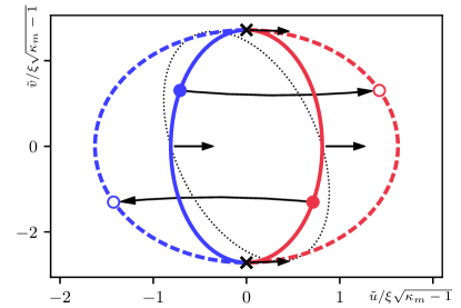
Figure 6: Jump line $\mathcal{J}_{\mathrm{\tilde{\bf R}}}$ (solid red/blue, see Eq. (54)) and landing line (dashed red/blue, see Eq. (63)) $\mathcal{L}_{\mathrm{\tilde{\bf R}}}$ in tip space $\tilde{\bf R}$ (in units of $\xi$), with the ellipse $\mathcal{J}_{\mathrm{\tilde{\bf R}}}$ representing the edge $\partial\mathcal{U}_{\tilde{\bf R}}$ of the unstable domain $\mathcal{U}_{\tilde{\bf R}}$. We choose parameters $\kappa_{m}-1=10^{-2}$, with $\lambda_{-}=-0.25\,e_{p}/\xi^{2},\lambda_{+}=0.05\,e_{p}/\xi^{2}$, and $a=0.07\,e_{p}/\xi^{3}$, $\alpha=0.1\,e_{p}/\xi^{4},\beta=0,\gamma=0.75\,e_{p}/\xi^{4}$ inspired by the choice of the uniaxial defect with 10 % anisotropy in Sec. IV; the dotted ellipse shows the effect of a finite skew parameter $\beta=0.05\,e_{p}/\xi^{4}$ on the jump ellipse $\mathcal{J}_{\mathrm{\tilde{\bf R}}}$. Along the edges of $\mathcal{U}_{\tilde{\bf R}}$, one of the stable tip configurations coalesces with the unstable solution of (38) and the total pinning energy $e_{\mathrm{pin}}(\tilde{\bf R};\bar{\bf R})$ develops an inflection line in the tip coordinate $\tilde{\bf R}$. Crosses correspond to the contact points (67) between the two ellipses $\mathcal{J}_{\mathrm{\tilde{\bf R}}}$ and $\mathcal{L}_{\mathrm{\tilde{\bf R}}}$. Blue and red colors identify different types of vortex deformations upon jump and landing. Pairs of solid and open circles connected via long arrows are, respectively, examples of pairs of jumping- and landing tip positions for vortices approaching the defect from the left (top) and right (bottom), see Fig. 5(c) for the isotropic problem’s counterpart. The unstable direction $\mathbf{v}_{-}(\tilde{\bf R}_{\mathrm{jp}})$, shown as short black arrows for different points on the ellipse, always points in the $u-$direction and are parallel to the tangent vector of the unstable ellipse at the contact points (67).

III.2.2 Landing line $\mathcal{L}_{\mathrm{\tilde{\bf R}}}$

We find the landing positions $\tilde{\bf R}_{\mathrm{lp}}$ by extending the discussion of the isotropic situation in Sec. II.4 to two dimensions: we shift the origin of the expansion (III.2.1) to the jump point $\tilde{\bf R}_{\mathrm{jp}}$ and find the landing point $\tilde{\bf R}_{\mathrm{lp}}=\tilde{\bf R}_{\mathrm{jp}}+\Delta\tilde{\bf R}$ by minimizing the total energy $e_{\mathrm{pin}}(\Delta\tilde{\bf R})$ at the landing position. Below, we use $\Delta\tilde{\bf R}$ both as a variable and as the jump distance to avoid introducing more coordinates.

We exploit the differential properties of $e_{\mathrm{pin}}$ at the jump and landing positions. At landing, $e_{\mathrm{pin}}(\tilde{\bf R}_{\mathrm{jp}}+\Delta\tilde{\bf R})$ has a minimum, hence, the configuration is force free, in particular along $\tilde{v}$,

$$\partial_{\tilde{v}}e_{\mathrm{pin}}(\tilde{\bf R}_{\mathrm{jp}}+\Delta\tilde{\bf R}) \approx[\partial_{\tilde{v}}\partial_{\tilde{u}}e_{\mathrm{pin}}]_{\tilde{\bf R}_{\mathrm{jp}}}\Delta\tilde{u}$$

$$\qquad+[\partial_{\tilde{v}}^{2}e_{\mathrm{pin}}]_{\tilde{\bf R}_{\mathrm{jp}}}\Delta\tilde{v}=0,$$

from which we find that $\Delta\tilde{u}$ and $\Delta\tilde{v}$ are related via

$$\Delta\tilde{v}\approx-\frac{[\partial_{\tilde{v}}\partial_{\tilde{u}}e_{\mathrm{pin}}]_{\tilde{\bf R}_{\mathrm{jp}}}}{[\partial_{\tilde{v}}^{2}e_{\mathrm{pin}}]_{\tilde{\bf R}_{\mathrm{jp}}}}\Delta\tilde{u}.$$ (59)

Here, we have dropped higher order terms in the expansion, assuming that the jump is mainly directed along the unstable $u$-direction—indeed, using the expansion (III.2.1), we find that

$$\Delta\tilde{v}\approx-\frac{a\tilde{v}_{\mathrm{jp}}}{\bar{C}+\lambda_{+}}\,\Delta\tilde{u}\propto\sqrt{\kappa_{m}-1}\>\Delta\tilde{u}.$$ (60)

Note that we cannot interchange the roles of $\tilde{u}$ and $\tilde{v}$ in this force analysis, as higher order terms in the expression for the force along $\tilde{u}$ cannot be dropped.

At the jump position $\tilde{\bf R}_{\mathrm{jp}}$, the state is force-free, i.e., the derivatives $[\partial_{\tilde{u}}e_{\mathrm{pin}}]_{\tilde{\bf R}_{\mathrm{jp}}}$ and $[\partial_{\tilde{v}}e_{\mathrm{pin}}]_{\tilde{\bf R}_{\mathrm{jp}}}$ vanish, and the Hessian determinant vanishes as well. Therefore, the expansion of $e_{\mathrm{pin}}(\tilde{\bf R}_{\mathrm{jp}}+\Delta\tilde{\bf R})$ has no linear terms and the second order terms $[\partial_{\tilde{u}}^{2}e_{\mathrm{pin}}]_{\tilde{\bf R}_{\mathrm{jp}}}\Delta\tilde{u}^{2}/2+[\partial_{\tilde{u}}\partial_{\tilde{v}}e_{\mathrm{pin}}]_{\tilde{\bf R}_{\mathrm{jp}}}\Delta\tilde{u}\Delta\tilde{v}+[\partial_{\tilde{v}}^{2}e_{\mathrm{pin}}]_{\tilde{\bf R}_{\mathrm{jp}}}\Delta\tilde{v}^{2}/2$ combined with Eq. (59) can be expressed through the Hessian determinant, $\{[\partial_{\tilde{u}}^{2}e_{\mathrm{pin}}][\partial_{\tilde{v}}^{2}e_{\mathrm{pin}}]-[\partial_{\tilde{u}}\partial_{\tilde{v}}e_{\mathrm{pin}}]^{2}\}_{\tilde{\bf R}_{\mathrm{jp}}}\Delta\tilde{u}^{2}/2=0$, that vanishes as well. Therefore, the expansion of $e_{\mathrm{pin}}$ around $\tilde{\bf R}_{\mathrm{jp}}$ starts at third order in $\Delta\tilde{\bf R}\approx(\Delta\tilde{u},0)$ and takes the form (we make use of (60), dropping terms $\propto\Delta\tilde{v}$ and a constant)

$$e_{\mathrm{pin}}(\tilde{\bf R}_{\mathrm{jp}}+\Delta\tilde{\bf R})\approx\frac{1}{6}\bigl{(}\gamma\tilde{u}_{\mathrm{jp}}+\beta\tilde{v}_{\mathrm{jp}}\bigr{)}\Delta\tilde{u}^{3}+\frac{\gamma}{24}\Delta\tilde{u}^{4}.$$ (61)

Minimizing this expression with respect to $\Delta\tilde{u}$ (as $e_{\mathrm{pin}}$ is minimal at $\tilde{\bf R}_{\mathrm{lp}}$), we obtain the result

$$\Delta\tilde{u}\approx-3(\gamma\tilde{u}_{\mathrm{jp}}+\beta\tilde{v}_{\mathrm{jp}})/\gamma.$$ (62)

Making use of the quadratic form (54), we can show that the equation for the landing position $\tilde{\bf R}_{\mathrm{lp}}=\tilde{\bf R}_{\mathrm{jp}}+\Delta\tilde{\bf R}$ can be cast into a similar quadratic form (with $\delta\tilde{\bf R}_{\mathrm{lp}}$ measured relative to $\tilde{\bf R}_{m}$)

$$\delta\tilde{\bf R}_{\mathrm{lp}}^{\mathrm{T}}M_{\mathrm{lp}}\,\delta\tilde{\bf R}_{\mathrm{lp}}=\bar{C}(\kappa_{m}-1),$$ (63)

but with the landing matrix now given by

$$M_{\mathrm{lp}}=\frac{1}{4}M_{\mathrm{jp}}+\begin{bmatrix}0&0\\ 0&~{}~{}~{}\displaystyle{\frac{3}{4}\Bigl{(}\frac{\delta}{2}-\frac{\beta^{2}}{2\gamma}\Bigr{)}}\end{bmatrix}.$$ (64)

In the following, we will refer to the solutions of Eq. (63) as the ‘landing’ or ‘stable’ ellipse $\tilde{\bf R}_{\mathrm{lp}}$ and write the jump distance in a parametric form involving the shape $\tilde{u}_{\mathrm{jp}}(\tilde{v})$ in Eq. (56) of the jumping ellipse,

$$\Delta\tilde{u}(\tilde{v})=-3\left[\gamma\,\tilde{u}_{\mathrm{jp}}(\tilde{v})+\beta\,\tilde{v}\right]/\gamma,$$ (65)

$$\Delta\tilde{v}(\tilde{v})=-\left[a/(\bar{C}+\lambda_{+})\right]\,\tilde{v}\,\Delta\tilde{u}(\tilde{v}).$$ (66)

The landing line derived from (63) is displayed as a dashed line in Fig. 6. Two tip jumps connected by an arrow are shown for illustration, with solid dots marking the jump position $\tilde{\bf R}_{\mathrm{jp}}$ of the tip and open dots its landing position $\tilde{\bf R}_{\mathrm{lp}}$; they describe tip jumps for a vortex approaching the unstable ellipse once from the left (upper pair) and another time from the right (lower pair). The different topologies associated with jumps and landing showing up for the isotropic defect in Fig. 5(c) (two concentric circles) and for the generic onset in Fig. 6 (two touching ellipses) will be discussed later.

Inspecting the matrix equation (63), we can gain several insights on the landing ellipse $\mathcal{L}_{\mathrm{\tilde{\bf R}}}$: (i) the matrix $M_{\mathrm{jp}}/4$ on the right-hand side of (64) corresponds to an ellipse with the same geometry as for $\mathcal{J}_{\mathrm{\tilde{\bf R}}}$ but double in size, (ii) the remaining matrix with vanishing entries in the off-diagonal and the $M_{xx}$ elements leaves the size doubling of the stable ellipse $\mathcal{L}_{\mathrm{\tilde{\bf R}}}$ at $\tilde{v}=0$ unchanged, and (iii) the finite $M_{yy}$ component exactly counterbalances the doubling along the $v-$direction encountered in (i), cf. the definiton (55) of $M_{\mathrm{jp}}$, up to a term proportional to the skew parameter $\beta$ accounting for deviations of the semiaxis from the $v-$axis. Altogether, the stable ellipse $\mathcal{L}_{\mathrm{\tilde{\bf R}}}$ extends with a double width along the $u-$axis and smoothly overlaps with the unstable ellipse at the two contact points $\tilde{v}_{c,\pm}$. The latter are found by imposing the condition $\Delta\tilde{u}=\Delta\tilde{v}=0$ in Eqs. (65) and (66); we find them located (relative to $\tilde{\bf R}_{m}$) at

$$\delta\tilde{\bf R}_{c,\pm} =\pm\left(-\beta/\gamma,1\right)\,\tilde{v}_{c},$$ (67)

with the endpoint coordinate $\tilde{v}_{c}$ given in Eq. (57), and mark them with crosses in Fig. 6. As anticipated, the contact points are off-set with respect to the $v-$axis for a finite skew parameter $\beta$. At these points, the unstable and the stable tip configurations coincide and the vortex tip undergoes no jump. Furthermore, the vector tangent to the jump (or landing) ellipse is parallel to the $u-$direction at the contact points. To see that, we consider (56) and find that

$$\frac{\partial\tilde{u}}{\partial\tilde{v}}\Big{|}_{\tilde{v}\to\pm\tilde{v}_{c}}\!\!\!\!\! \approx\pm\left(\sqrt{\tilde{v}_{c}^{2}-\frac{2\gamma\,\bar{C}(\kappa_{m}-1)}{\gamma\beta-\delta^{2}}}\right)^{-1}\!\!\!\to\pm\infty,$$ (68)

hence, the corresponding tangents $\partial_{\tilde{u}}\tilde{v}$ vanish.

The asymptotic positions $\bar{\bf R}$ where the vortex tips jump and land belong to the boundary of the bistable region $\mathcal{B}_{\bar{\bf R}}$; for the isotropic case in Fig. 5(d) these correspond to the circles with radii $\bar{R}_{-}$ (pinning) and $\bar{R}_{+}$ (depinning) with jump and landing radii $\tilde{R}_{\mathrm{f-}}(\bar{R}_{-})$ and $\tilde{R}_{\mathrm{p-}}(\bar{R}_{-})$ and $\tilde{R}_{\mathrm{p+}}(\bar{R}_{+})$ and $\tilde{R}_{\mathrm{f+}}(\bar{R}_{+})$, respectively, see Fig. 5(c). For the anisotropic defect, we have only a single jump/landing event at one asymptotic position $\bar{\bf R}$ that we are going to determine in the next section.

III.3 Bistable domain $\mathcal{B}_{\bar{\bf R}}$

The set of asymptotic positions $\bar{\bf R}$ corresponding to the tip positions $\tilde{\bf R}_{\mathrm{jp}}$ along the edges of $\mathcal{U}_{\tilde{\bf R}}$ forms the boundary $\partial\mathcal{B}_{\bar{\bf R}}$ of the bistable domain $\mathcal{B}_{\bar{\bf R}}$; they are related through the force-balance equation (38), with every vortex tip position $\tilde{\bf R}_{\mathrm{jp}}\in\partial\mathcal{U}_{\tilde{\bf R}}$ defining an associated asymptotic position $\bar{\bf R}(\tilde{\bf R}_{\mathrm{jp}})\in\partial\mathcal{B}_{\bar{\bf R}}$.

At the onset of strong pinning, the bistable domain corresponds to the isolated point $\bar{\bf R}_{m}$, related to $\tilde{\bf R}_{m}$ through (38). Beyond the Labusch point, $\mathcal{B}_{\bar{\bf R}}$ expands out of $\bar{\bf R}_{m}$ and its geometry is found by evaluating the force balance equation (38) at a given tip position $\tilde{\bf R}_{\mathrm{jp}}\in\partial\mathcal{U}_{\tilde{\bf R}}$, $\bar{\bf R}(\tilde{\bf R}_{\mathrm{jp}})=\tilde{\bf R}_{\mathrm{jp}}-\mathbf{f}_{p}(\tilde{\bf R}_{\mathrm{jp}})/\bar{C}\in\partial\mathcal{B}_{\bar{\bf R}}$. Using the expansion (III.2.1) for $e_{\mathrm{pin}}(\tilde{\bf R};\bar{\bf R})$, this force equation can be expressed as $\nabla_{\mathbf{R}}e_{\mathrm{pin}}(\mathbf{R};\bar{\bf R})\big{|}_{\tilde{\bf R}}=0$, or explicitly (we remind that we measure $\bar{\bf R}=\bar{\bf R}_{m}+(\bar{u},\bar{v})$ relative to $\bar{\bf R}_{m}$),

$$\bar{C}\bar{u} =\bar{C}(1-\kappa_{m})\tilde{u}+\frac{a}{2}\tilde{v}^{2}+\frac{\gamma}{6}\tilde{u}^{3}+\frac{\beta}{2}\tilde{u}^{2}\tilde{v}+\frac{\alpha}{2}\tilde{u}\tilde{v}^{2},$$

$$\bar{C}\bar{v} =(\bar{C}+\lambda_{+})\tilde{v}+a\,\tilde{u}\tilde{v}+\frac{\beta}{6}\tilde{u}^{3}+\frac{\alpha}{2}\tilde{u}^{2}\tilde{v}.$$ (69)

Inserting the results for the jump ellipse $\mathcal{J}_{\mathrm{\tilde{\bf R}}}$, Eq. (56), into Eqs. (69), we find the crescent-shape bistable domain $\mathcal{B}_{\bar{\bf R}}$ shown in Fig. 7; let us briefly derive the origin of this shape.

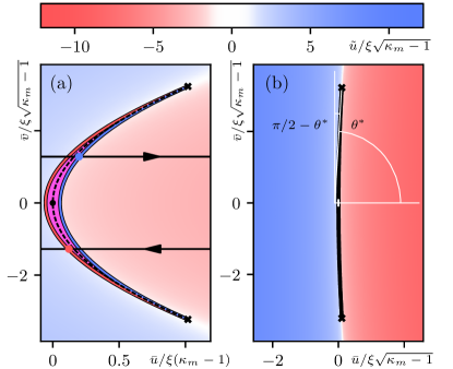
Figure 7: (a) Bistable domain $\mathcal{B}_{\bar{\bf R}}$ in asymptotic $\bar{\bf R}$-space measured in units of $\xi$; the same parameters as in Fig. 6 have been used. Note the different scaling of the axes in $\kappa_{m}-1$; the right panel (b) shows $\mathcal{B}_{\bar{\bf R}}$ in isotropic scales. The bistable domain $\mathcal{B}_{\bar{\bf R}}$ is elongated along the transverse direction $\bar{v}$ and narrow/bent along the unstable direction $\bar{u}$, giving $\mathcal{B}_{\bar{\bf R}}$ its peculiar crescent-like shape. The branch crossing line $\bar{\bf R}_{0}$, see (77), is shown as a dashed black line. Black crosses mark the cusps of $\mathcal{B}_{\bar{\bf R}}$ and are associated with the contact points of $\mathcal{U}_{\tilde{\bf R}}$ through the force balance equation (38); they correspond to critical end-points in the thermodynamic Ising analogue, while the boundaries $\partial\mathcal{B}_{\bar{\bf R}}$ map to spinodals. Blue and red colors identify different characters of vortex tip configurations as quantified through the ‘order parameter’ $\tilde{u}$ of the Landau expansion (at $\beta=0$), see text, while magenta is associated to the bistable area $\mathcal{B}_{\bar{\bf R}}$; the blue and red branches extend to the far side of the crescent and terminate in the blue and red colored boundaries $\partial\mathcal{B}_{\bar{\bf R}}^{\mathrm{b}}$ and $\partial\mathcal{B}_{\bar{\bf R}}^{\mathrm{r}}$, respectively. Thin horizontal lines show vortex trajectories that proceed smoothly in asymptotic space, see also Fig. 5(d). Blue and red dots mark the asymptotic positions associated with vortex tip jumps that happen at the exit of $\mathcal{B}_{\bar{\bf R}}$; they correspond to the pairs of tip positions in Fig. 6. (b) Bistable domain $\mathcal{B}_{\bar{\bf R}}$ in isotropic scaled coordinates $\bar{u}$ and $\bar{v}$ showing the ‘true’ shape of $\mathcal{B}_{\bar{\bf R}}$. Vortices impacting on the bistable domain with an angle $|\theta|\leq\theta^{\ast}$ undergo a single jump on the far side of $\mathcal{B}_{\bar{\bf R}}$, with the pinning force density directed along $u$ and scaling as $F_{\mathrm{pin}}^{\parallel}\propto(\kappa-1)^{5/2}$. Vortices crossing $\mathcal{B}_{\bar{\bf R}}$ at large angles close to $\pi/2$ jump either never, once, or twice; at $\theta=\pi/2$ the pinning force density is small, $F_{\mathrm{pin}}^{\perp}\propto(\kappa-1)^{3}$, and directed along $v$.

Solving (69) to leading order, $\bar{C}\bar{u}^{\scriptscriptstyle(0)}\approx(a/2)\tilde{v}^{2}$ and $\bar{C}\bar{v}^{\scriptscriptstyle(0)}\approx(\bar{C}+\lambda_{+})\tilde{v}$, we find the parabolic approximation

$$\bar{u}^{\scriptscriptstyle(0)} \approx\frac{a}{2\bar{C}}\frac{1}{(1+\lambda_{+}/\bar{C})^{2}}\,\bar{v}^{{\scriptscriptstyle(0)}\,2},$$ (70)

telling that the extent of $\mathcal{B}_{\bar{\bf R}}$ scales as $(\kappa_{m}-1)$ along $\bar{u}$ and $\propto(\kappa_{m}-1)^{1/2}$ along $\bar{v}$, i.e., we find a flat parabola opening towards positive $\bar{u}$ for $a>0$, see Fig. 7.

In order to find the width of $\mathcal{B}_{\bar{\bf R}}$, we have to solve (69) to the next higher order, $\bar{u}=\bar{u}^{\scriptscriptstyle(0)}+\bar{u}^{\scriptscriptstyle(1)}$; for $\beta=0$, we find the correction

$$\bar{u}^{\scriptscriptstyle(1)}=(1-\kappa_{m})\tilde{u}+\frac{\gamma}{6\bar{C}}\tilde{u}^{3}+\frac{\alpha}{2\bar{C}}\tilde{u}\tilde{v}^{2}$$ (71)

that produces a $\bar{v}\leftrightarrow-\bar{v}$ symmetric crescent. Inserting the two branches (56) of the jump ellipse, we arrive at the width of the crescent that scales as $(\kappa_{m}-1)^{3/2}$. The correction to $\bar{v}$ is $\propto(\kappa_{m}-1)$ and we find the closed form

$$\bar{v} \approx[1+(\lambda_{+}+a\tilde{u})/\bar{C}]\>\tilde{v}$$ (72)

with a small antisymmetric (in $\tilde{u}$) correction. For a finite $\beta\neq 0$, the correction $\bar{u}^{\scriptscriptstyle(1)}$ picks up an additional term $(\beta/2\bar{C})\,\tilde{u}^{2}\tilde{v}$ that breaks the $\bar{v}\leftrightarrow-\bar{v}$ symmetry and the crescent is distorted.

Viewing the boundary $\partial\mathcal{B}_{\bar{\bf R}}$ as a parametric curve in the variable $\tilde{v}$ with $\tilde{u}=\tilde{u}_{\mathrm{jp}}(\tilde{v})$ given by Eq. (56), we obtain the boundary $\partial\mathcal{B}_{\bar{\bf R}}$ in the form of two separate arcs that define the crescent-shaped domain $\mathcal{B}_{\bar{\bf R}}$ in Fig. 7(a). The two arcs merge in two cusps at $\bar{\bf R}_{c,\pm}$ that are associated to the touching points (67) in dual space and derive from Eqs. (69); measured with respect to $\bar{\bf R}_{m}$, these cusps are located at

$$\delta\bar{\bf R}_{c,\pm} = (\bar{u}_{c},\pm\bar{v}_{c})$$

$$\approx \left[\left(a/2\,\bar{C}\right)\,\tilde{v}^{2}_{c},\,\pm(1+\lambda_{+}/\bar{C})\tilde{v}_{c}\right].$$

The coloring in Fig. 7 indicates the characters ‘red’ and ‘blue’ of the vortex states; these are defined in terms of the ‘order parameter’ $\tilde{u}-\tilde{u}_{m}(\bar{v})$ of the Landau functional (III.2.1) that changes sign at the branch crossing line Eq. (77), with the shift

$$\tilde{u}_{m}(\bar{v})=-\frac{\beta}{\gamma}\tilde{v}(\bar{v})\approx-\frac{\beta}{\gamma}\frac{\bar{v}}{1+\lambda_{+}/\bar{C}},$$ (74)

$\tilde{u}_{m}(\bar{v})=0$ for our symmetric case with $\beta=0$ in Fig. 7. Going beyond the cusps (or critical points) at $\bar{\bf R}_{c,\pm}$, the two states smoothly crossover between ‘red’ and ‘blue’ (indicated by the smooth blue–white–red transition), as known for the van der Waals gas (or Ising magnet) above the critical point. Within the bistable region $\mathcal{B}_{\bar{\bf R}}$, both ‘red’ and ‘blue’ states coexist and we color this region in magenta.

The geometry of the bistable domain $\mathcal{B}_{\bar{\bf R}}$ is very different from the ring-shaped geometry of the isotropic problem discussed in Sec. II.1, see Fig. 5(d); in the discussion of the uniaxial anisotropic defect below, we will learn how these two geometries are interrelated. Comparing the overall dimensions of the crescent with the ring in Fig. 5(d), we find the following scaling behavior in $\kappa_{m}-1$: while the crescent $\mathcal{B}_{\bar{\bf R}}$ grows along $\bar{v}$ as $(\kappa_{m}-1)^{1/2}$, the isotropic ring involves the characteristic size $\xi$ of the defect, $\bar{R}_{-}\sim\xi$ and hence its extension along $\bar{v}$ is a constant. On the other hand, the scaling of the crescent’s and the ring’s width is the same, $\propto(\kappa_{m}-1)^{3/2}$. The different scaling of the transverse width then will be responsible for the new scaling of the pinning force density, $F_{\mathrm{pin}}\propto(\kappa_{m}-1)^{5/2}$.

III.4 Comparison to isotropic situation

Let us compare the unstable domains $\mathcal{U}_{\tilde{\bf R}}$ for the isotropic and anisotropic defects in Figs. 5(c) and 6, respectively. In the isotropic example of Sec. II.1, the jump- and landing-circles $\tilde{R}_{\mathrm{jp}}(\bar{R})$ and $\tilde{R}_{\mathrm{lp}}(\bar{R})$ are connected to different phases, e.g., free (colored in blue at $\tilde{R}_{\mathrm{jp}}=\tilde{R}_{\mathrm{f-}}$) and pinned (colored in red at $\tilde{R}_{\mathrm{lp}}=\tilde{R}_{\mathrm{p-}}$) associated with $\bar{R}_{-}$. Furthermore, the topology is different, with the unstable ring domain separating the two distinct phases, free and pinned ones. As a result, a second pair of jump- and landing-positions associated with the asymptotic circle $\bar{R}_{+}$ appears along the vortex trajectory of Fig. 5(c); these are the located at the radii $\tilde{R}_{\mathrm{jp}}=\tilde{R}_{\mathrm{p+}}$ and $\tilde{R}_{\mathrm{lp}}=\tilde{R}_{\mathrm{f+}}$ and describe the depinning process from the pinned branch back to the free branch (while the previous pair at radii $\tilde{R}_{\mathrm{f-}}$ and $\tilde{R}_{\mathrm{p-}}$ describes the pinning process from the free to the pinned branch). The pinning (at $\bar{R}_{-}$) and depinning (at $\bar{R}_{+}$) processes in the asymptotic coordinates are shown in figure 5(d). The bistable area $\mathcal{B}_{\bar{\bf R}}$ with coexisting free and pinned states has a ring-shape as well (colored in magenta, the superposition of blue and red); the two pairs of jump and landing points in tip space have collapsed to two pinning and depinning points in asymptotic space.

In the present situation describing the strong pinning onset for a generic anisotropic potential, the unstable domain $\mathcal{U}_{\tilde{\bf R}}$ grows out of an isolated point (in fact, $\tilde{\bf R}_{m}$) and assumes the shape of an ellipse that is simply connected; as a result, a vortex incident on the defect undergoes only a single jump, see Fig. 6. The bistable domain $\mathcal{B}_{\bar{\bf R}}$ is simply connected as well, but now features two cusps at the end-points of the crescent, see Fig. 7. The bistability again involves two states, but we cannot associate them with separated pinned and free phases—we thus denote them by ‘blue’-type and ‘red’-type. The two states approach one another further away from the defect and are distiguishable only in the region close to bistability; in Fig. 7, this is indicated with appropriate color coding. Note that the Landau-type expansion underlying the coloring in Fig. 7 fails at large distances; going beyond a local expansion near $\tilde{\bf R}_{m}$, the distortion of the vortex vanishes at large distances and red/blue colors faint away to approach ‘white’.

III.5 Topology

The different topologies of unstable and bistable regions appearing in the isotropic and anisotropic situations are owed to the circular symmetry of the isotropic defect; we will recover the ring-like topology for the anisotropic situation later when describing a uniaxially anisotropic defect at larger values of the Labusch parameter $\kappa_{m}$. Indeed, such an increase in pinning strength will induce a change in topology with two crescents facing one another joining into a ring-like shape.

Let us discuss the consequences of the different topologies that we encountered for the isotropic and anisotropic defects in the discussion above. Specifically, the precise number and position of the contact points have an elegant topological explanation. When a vortex tip touches the edges $\tilde{\bf R}_{\mathrm{jp}}$ of the unstable domain there are two characteristic directions: one is given by the unstable eigenvector $\mathbf{v}_{-}(\tilde{\bf R}_{\mathrm{jp}})$ discussed in Sec. III.2 along which the tip will jump initially. The second is the tangent vector to the boundary $\partial\mathcal{U}_{\tilde{\bf R}}$ of the unstable domain, i.e., to the unstable ellipse. While the former is approximately constant and parallel to the unstable $u$-direction along $\tilde{\bf R}_{\mathrm{jp}}$, the latter winds around the ellipse exactly once after a full turn around $\mathcal{U}_{\tilde{\bf R}}$. The contact points $\tilde{\bf R}_{c,\pm}$ of the unstable and stable ellipses then coincide with those points on the ellipse where the tangent vector are parallel and anti-parallel to $\mathbf{v}_{-}$; at these points, the tip touches the unstable ellipse but does not undergo a jump any more. Given the different winding numbers of $\mathbf{v}_{-}$ and of the tangent vector, there are exactly two points along the circumference of $\mathcal{U}_{\tilde{\bf R}}$ where the tangent vector is parallel/anti-parallel to the $u$-direction; these are the points found in (67). This argument remains valid as long as the contour $\partial\mathcal{U}_{\tilde{\bf R}}$ is not deformed to cross/encircle the singular point of the $\mathbf{v}_{-}(\tilde{\bf R}_{\mathrm{jp}})$ field residing at the defect center.

The same arguments allow us to understand the absence of contact points in the isotropic scenario: For an isotropic potential, the winding number $n_{\scriptscriptstyle\mathcal{U}}$ of the tangent vector around $\mathcal{U}_{\tilde{\bf R}}$ remains unchanged, i.e., $n_{\scriptscriptstyle\mathcal{U}}=\pm 1$, while the unstable direction $\mathbf{v}_{-}$ is pointing along the radius and thus acquires a unit winding number as well. Indeed, the two directions, tangent and jump, then rotate simultaneously and do not wind around each other after a full rotation, explaining the absence of contact points in the isotropic situation.

III.6 Energy jumps

Within strong pinning theory, the energy jump $\Delta e_{\mathrm{pin}}$ associated with the vortex tip jump between bistable vortex configurations at the boundaries of $\mathcal{B}_{\bar{\bf R}}$ determines the pinning force density $F_{\mathrm{pin}}$ and the critical current $j_{c}$, see Eqs. (16) and (17). Formally, the energy jump $\Delta e_{\mathrm{pin}}$ is defined as the difference in energy $e_{\mathrm{pin}}(\tilde{\bf R};\bar{\bf R})$ at fixed asymptotic position $\bar{\bf R}\in\partial\mathcal{B}_{\bar{\bf R}}$ between vortex configurations with tips in the jump ($\tilde{\bf R}_{\mathrm{jp}}(\bar{\bf R})$) and landing ($\tilde{\bf R}_{\mathrm{lp}}(\bar{\bf R})=\tilde{\bf R}_{\mathrm{jp}}(\bar{\bf R})+\Delta\tilde{\bf R}$) positions,

$$\Delta e_{\mathrm{pin}}(\bar{\bf R}\in\partial\mathcal{B}_{\bar{\bf R}})\equiv e_{\mathrm{pin}}[\tilde{\bf R}_{\mathrm{jp}}(\bar{\bf R});\bar{\bf R}]\\ -e_{\mathrm{pin}}[\tilde{\bf R}_{\mathrm{lp}}(\bar{\bf R});\bar{\bf R}].$$ (75)

In Sec. III.2.2 above, we have found that the jump $\Delta\tilde{\bf R}$ is mainly forward directed along $u$. Making use of the expansion (61) of $e_{\mathrm{pin}}$ at $\tilde{\bf R}_{\mathrm{jp}}$ and the result (62) for the jump distance $\Delta\tilde{u}$, we find the energy jumps $\Delta e_{\mathrm{pin}}$ in tip- and asymptotic space in the form (cf. with the isotropic result Eq. (24)),

$$\Delta e_{\mathrm{pin}}(\bar{\bf R}) \approx\frac{\gamma}{72}\Delta\tilde{u}^{4}\approx\left(\frac{9}{8\gamma^{3}}\right)\left[\gamma\,\tilde{u}_{\mathrm{jp}}(\tilde{v})+\beta\,\tilde{v}\right]^{4}$$ (76)

$$\approx\left(\frac{9}{8\gamma^{3}}\right)\left[(\gamma\delta-\beta^{2})\left(\tilde{v}_{c}^{2}-\tilde{v}^{2}\right)\right]^{2}$$

$$\approx\left(\frac{9}{8\gamma^{3}}\right)\left[\frac{(\gamma\delta-\beta^{2})}{(1+\lambda_{+}/\bar{C})^{2}}\left(\bar{v}_{c}^{2}-\bar{v}^{2}\right)\right]^{2}.$$

Here, we have used the parametric shape $\tilde{u}_{\mathrm{jp}}(\tilde{v})$ in Eq. (56) for the jumping ellipse as well as (69) to lowest order, $\tilde{v}\approx\bar{v}/(1+\lambda_{+}/\bar{C})$, to relate the tip and asymptotic positions in the last equation. The energy jump (76) scales as $(\kappa_{m}-1)^{2}$ and is shown in Fig. 8. It depends on the $v$ coordinate of the asymptotic (or tip) position only and vanishes at the cusps $\bar{\bf R}_{c,\pm}$, see Eq. (III.3) (or at the touching points $\tilde{\bf R}_{c,\pm}$, see Eq. (67)). To order $(\kappa_{m}-1)^{2}$, the energy jumps are identical at the left and right edges of the bistable domain $\mathcal{B}_{\bar{\bf R}}$.

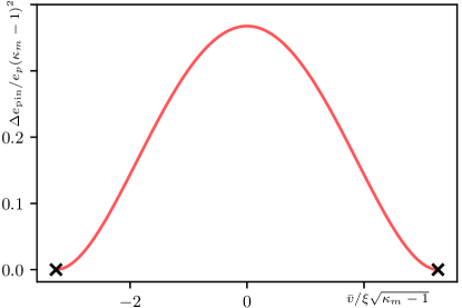
Figure 8: Energy jump $\Delta e_{\mathrm{pin}}$ along the edges of the bistable domain $\mathcal{B}_{\bar{\bf R}}$ as a function of the transverse coordinate $\bar{v}$; we have used the same parameters as in Fig. 6. The energy jump vanishes at the cusps $\pm\bar{v}_{c}$, as the bistable tip configurations become identical and their energies turn equal.

Following the two bistable branches and the associated energy jumps between them to the inside of $\mathcal{B}_{\bar{\bf R}}$, the latter vanish along the branch crossing line $\bar{\bf R}_{0}$. In the thermodynamic analogue, this line corresponds to the first-order equilibrium transition line that is framed by the spinodal lines; for the isotropic defect, this is the circle with radius $\bar{R}_{0}=x_{0}$ framed by the spinodal circles with radii $\bar{R}_{\pm}$, see Figs. 4 and 5(d). For the anisotropic defect with $\beta=0$, this line is trivially given by the centered parabola of $\mathcal{B}_{\bar{\bf R}}$, see Eq. (70), and hence

$$\bar{u}_{0}\approx\frac{a}{2\bar{C}}\frac{1}{(1+\lambda_{+}/\bar{C})^{2}}\bar{v}_{0}^{2}.$$ (77)

The result for a finite skew parameter $\beta\neq 0$ is given by Eq. (175) in Appendix A.1.

III.7 Pinning force density

The pinning force density $F_{\mathrm{pin}}$ is defined as the average force density exerted on a vortex line as it moves across the superconducting sample. For the isotropic case described in Sec. II.5, the individual pinning force $\mathbf{f}_{\mathrm{pin}}(\bar{\bf R})=-\nabla_{\bar{\bf R}}e_{\mathrm{pin}}(\bar{\bf R})$, see Eq. (7), is directed radially and the force density $F_{\mathrm{pin}}$ is given by the (constant) energy jump $\Delta e_{\mathrm{pin}}\propto(\kappa-1)^{2}$ on the edge $\partial\mathcal{B}_{\bar{\bf R}}$ of the bistable domain and the transverse length $t_{\perp}\sim\xi$, hence, $F_{\mathrm{pin}}\propto t_{\perp}\Delta e_{\mathrm{pin}}$ scales as $(\kappa-1)^{2}$.

For an anisotropic defect, the pinning force depends on the vortex direction of motion $\hat{\mathbf{v}}=(\cos\theta,\sin\theta)$ relative to the axis of the bistable region: we choose angles $-\pi/2\leq\theta\leq\pi/2$ measured from the unstable direction $\bar{u}$, i.e., vortices incident from the left; the case of larger impact angles $|\theta|>\pi/2$ corresponds to vortices incident from the right and can be reduced to the previous case by inverting the sign of the parameter $a$ in the expansion (III.2.1), i.e., the curvature of the parabola (70); to our leading order analysis, the results remain the same. The pinning force is no longer directed radially but depends on $\theta$; furthermore, the energy jump (76) is non-uniform along the boundary $\mathcal{B}_{\bar{\bf R}}$.

In spite of these complications, we can perform some simple scaling estimates as a first step: let us assume a uniform distribution of identical anisotropic defects, all with their unstable direction pointing along $x$. The jumps in energy still scale as $\Delta e_{\mathrm{pin}}\propto(\kappa_{m}-1)^{2}$, however, the trapping distance is no longer finite but grows from zero as $\kappa_{m}-1$ increases. Due to their elongated shapes, the bistable domains $\mathcal{B}_{\bar{\bf R}}$ exhibit different extensions along the $y$ and $x$ directions, i.e., $\propto\bar{v}_{c}\propto\sqrt{\kappa_{m}-1}$ along $y$ and $\propto\bar{u}_{c}\propto(\kappa_{m}-1)$ along $x$, respectively. These simple considerations then suggest that the pinning force density exhibits a scaling $F_{\mathrm{pin}}\propto(\kappa_{m}-1)^{\mu}$ with $\mu>2$, different from the setup with isotropic defects. Even more, vortices moving along the $x$ or $y$ directions, respectively, will experience different forces $F_{\mathrm{pin}}^{\parallel}$ and $F_{\mathrm{pin}}^{\perp}$ scaling as

$$F_{\mathrm{pin}}^{\parallel}\propto(\kappa_{m}-1)^{5/2},\quad F_{\mathrm{pin}}^{\perp}\propto(\kappa_{m}-1)^{3}$$ (78)

near the onset of strong pinning. While such uniform anisotropic defects could be created artificially, a more realistic scenario will involve defects that are randomly oriented and an additional averaging over angles $\theta$ has to be performed; this will be done at the end of this section.

We first determine the magnitude and orientation of the pinning force density $\mathbf{F}_{\mathrm{pin}}(\theta)$ as a function of the vortex impact angle $\theta$ for randomly positioned but uniformly oriented (along $x$) defects of density $n_{p}$. The pinning force density is given by the average over relative positions between vortices and defects (with a minus sign following convention; $\mathcal{V}_{\bar{\bf R}}$ denotes the vortex lattice unit cell),

$$\mathbf{F}_{\mathrm{pin}}(\theta)=-n_{p}\int_{\mathcal{V}_{\bar{\bf R}}\setminus\mathcal{B}_{\bar{\bf R}}}\!\!\frac{\mathrm{d}^{2}\bar{\bf R}}{a_{0}^{2}}\,\mathbf{f}_{\mathrm{pin}}(\bar{\bf R})$$ (79)

$$\quad-n_{p}\int_{\mathcal{B}_{\bar{\bf R}}}\!\!\!\frac{\mathrm{d}^{2}\bar{\bf R}}{a_{0}^{2}}\left[p_{\mathrm{b}}(\bar{\bf R};\theta)\,\mathbf{f}^{\mathrm{b}}_{\mathrm{pin}}(\bar{\bf R})+p_{\mathrm{r}}(\bar{\bf R};\theta)\,\mathbf{f}^{\mathrm{r}}_{\mathrm{pin}}(\bar{\bf R})\right].$$

Outside of the bistable domain, i.e., in $\mathcal{V}_{\bar{\bf R}}\setminus\mathcal{B}_{\bar{\bf R}}$, a single stable vortex tip configuration exists and the pinning force $\mathbf{f}_{\mathrm{pin}}(\bar{\bf R})$ is uniquely defined. Inside $\mathcal{B}_{\bar{\bf R}}$, the branch occupation functions $p_{\mathrm{b,r}}(\bar{\bf R};\theta)$ are associated with the tip positions appertaining to the ‘blue’ and the ‘red’ vortex configurations with different tip positions $\tilde{\bf R}^{\mathrm{b,r}}(\bar{\bf R})$, cf. Figs. 6 and 7. The pinning forces $\mathbf{f}^{\mathrm{b,r}}_{\mathrm{pin}}(\bar{\bf R})$ are evaluated for the corresponding vortex tip positions and are defined as

$$\mathbf{f}^{\mathrm{b,r}}_{\mathrm{pin}}(\bar{\bf R})=-\mathbf{\nabla}_{\bar{\bf R}}e_{\mathrm{pin}}[\tilde{\bf R}^{\mathrm{b,r}}(\bar{\bf R});\bar{\bf R}].$$ (80)

Let us now study how vortex lines populate the bistable domain as a function of the impact angle $\theta$. Examining Fig. 7, we can distinguish between two different angular regimes: a frontal-impact regime at angles away from $\pi/2$, $|\theta|\leq\theta^{\ast}$, where all the vortices that cross the bistable domain undergo exactly one jump on the far edge of $\mathcal{B}_{\bar{\bf R}}$, see the blue dot and blue boundary $\partial\mathcal{B}_{\bar{\bf R}}^{\mathrm{b}}$ in Fig. 7; and a transverse regime for angles $\theta^{\ast}\leq|\theta|\leq\pi/2$, where vortices crossing the bistable domain undergo either no jump, one or two. The angle $\theta^{\ast}$ is given by the (outer) tangent of the bistable domain at the cusps $\bar{\bf R}_{c,\pm}$; making use of the lowest order approximation (70) of the crescent’s geometry, we find that

$$\tan(\theta^{\ast}) =\frac{\partial\bar{v}^{\scriptscriptstyle(0)}}{\partial\bar{u}^{\scriptscriptstyle(0)}}\Big{|}_{\bar{v}_{c}}=\frac{(\bar{C}+\lambda_{+})}{a}\sqrt{\frac{\gamma\delta-\beta^{2}}{2\gamma\bar{C}(\kappa_{m}-1)}},$$ (81)

implying that $\pi/2-\theta^{\ast}\propto\sqrt{\kappa_{m}-1}$ is small,

$$\theta^{\ast}\approx\pi/2-\frac{a}{(\bar{C}+\lambda_{+})}\sqrt{\frac{2\gamma\bar{C}(\kappa_{m}-1)}{\gamma\delta-\beta^{2}}}.$$ (82)

III.7.1 Impact angles $|\theta|<\theta^{\ast}$

For a frontal impact with $|\theta|<\theta^{\ast}$, vortices occupy the ‘blue’ branch and remain there throughout the bistable domain $\mathcal{B}_{\bar{\bf R}}$ until its termination on the far edge $\partial\mathcal{B}_{\bar{\bf R}}^{\mathrm{b}}$, see Fig. 7, implying that $p_{\mathrm{b}}(\bar{\bf R}\in\mathcal{B}_{\bar{\bf R}})=1$ and $p_{\mathrm{r}}(\bar{\bf R}\in\mathcal{B}_{\bar{\bf R}})=0$, independent of $\theta$. As a consequence, the pinning force $\mathbf{F}_{\mathrm{pin}}$ does not depend an the impact angle and is given by the expression

$$\mathbf{F}^{<}_{\mathrm{pin}}=-n_{p}\!\int_{\mathcal{V}_{\bar{\bf R}}\setminus\mathcal{B}_{\bar{\bf R}}}\!\!\!\!\frac{\mathrm{d}^{2}\bar{\bf R}}{a_{0}^{2}}\,\mathbf{f}_{\mathrm{pin}}(\bar{\bf R})-n_{p}\!\int_{\mathcal{B}_{\bar{\bf R}}}\!\!\!\!\frac{\mathrm{d}^{2}\bar{\bf R}}{a_{0}^{2}}\,\mathbf{f}^{\mathrm{b}}_{\mathrm{pin}}(\bar{\bf R}).$$

Next, Gauss’ formula tells us that for a function $e(\mathbf{x})$, we can transform

$$\int_{\mathcal{V}}\mathrm{d}^{n}x\,\mathbf{\nabla}e(\mathbf{x})=\int_{\partial\mathcal{V}}\mathrm{d}^{n-1}\,\mathbf{S}_{\perp}\,e(\mathbf{x}),$$ (83)

with the surface element $\mathrm{d}^{n-1}\,\mathbf{S}_{\perp}$ oriented perpendicular to the surface and pointing outside of the domain $\mathcal{V}$. In applying (83) to the first integral of $\mathbf{F}^{<}_{\mathrm{pin}}$, we can drop the contribution from the outer boundary $\partial\mathcal{V}_{\bar{\bf R}}$ since we assume a compact defect potential. The remaining contribution from the crescent’s boundary $\partial\mathcal{B}_{\bar{\bf R}}$ joins up with the second integral but with an opposite sign, as the two terms involve the same surface but with opposite orientations. Altogether, we then arrive at the expression

$$\mathbf{F}^{<}_{\mathrm{pin}}=n_{p}\int_{\partial\mathcal{B}_{\bar{\bf R}}^{\mathrm{b}}}\frac{\mathrm{d}\,\mathbf{S}_{\perp}}{a_{0}^{2}}\left(e^{\mathrm{b}}_{\mathrm{pin}}(\bar{\bf R})-e_{\mathrm{pin}}(\bar{\bf R})\right)\\ +n_{p}\int_{\partial\mathcal{B}_{\bar{\bf R}}^{\mathrm{r}}}\frac{\mathrm{d}\,\mathbf{S}_{\perp}}{a_{0}^{2}}\left(e^{\mathrm{b}}_{\mathrm{pin}}(\bar{\bf R})-e_{\mathrm{pin}}(\bar{\bf R})\right),$$ (84)

where we have separated the left and right borders $\partial\mathcal{B}_{\bar{\bf R}}^{\mathrm{r,b}}$ of the bistable domain. Due to continuity, the stable vortex energy $e_{\mathrm{pin}}(\bar{\bf R})$ will be equal to $e_{\mathrm{pin}}^{\mathrm{b}}(\bar{\bf R})$ on the left border $\partial\mathcal{B}_{\bar{\bf R}}^{\mathrm{r}}$ and equal to $e_{\mathrm{pin}}^{\mathrm{r}}(\bar{\bf R})$ on the right border $\partial\mathcal{B}_{\bar{\bf R}}^{\mathrm{b}}$. The expression (84) for $\mathbf{F}^{<}_{\mathrm{pin}}$ then reduces to

$$\mathbf{F}^{<}_{\mathrm{pin}} =n_{p}\int_{\partial\mathcal{B}_{\bar{\bf R}}^{\mathrm{b}}}\frac{\mathrm{d}\,\mathbf{S}_{\perp}}{a_{0}^{2}}\left(e^{\mathrm{b}}_{\mathrm{pin}}(\bar{\bf R})-e^{\mathrm{r}}_{\mathrm{pin}}(\bar{\bf R})\right)$$

$$=n_{p}\int_{-\bar{v}_{c}}^{\bar{v}_{c}}\frac{\mathrm{d}\bar{v}}{a_{0}}\,\frac{\Delta e_{\mathrm{pin}}(\bar{v})}{a_{0}}\left[1,-\partial{\bar{u}}/\partial{\bar{v}}\right]$$

$$=n_{p}\left[\frac{2\bar{v}_{c}}{a_{0}}\frac{\langle\Delta e_{\mathrm{pin}}\rangle}{a_{0}},\,0\right]\equiv[F^{\parallel}_{\mathrm{pin}},0]$$ (85)

with $\langle\Delta e_{\mathrm{pin}}\rangle$ the average energy jump evaluated along the $v$-direction. The force $\mathbf{F}^{<}_{\mathrm{pin}}$ is aligned with the unstable directed along $u$, with the $v$-component vanishing due to the antisymmetry in $\bar{v}\leftrightarrow-\bar{v}$ of the derivative $\partial{\bar{u}}/\partial{\bar{v}}$, and is independent on $\theta$ for $|\theta|<\theta^{*}$.

III.7.2 Impact angle $|\theta|=\pi/2$

Second, let us find the pinning force density $\mathbf{F}^{\pi/2}_{\mathrm{pin}}$ for vortices moving along the (positive) $v$-direction, $\theta=\pi/2$. As follows from Fig. 7, vortices occupy the blue branch and jump to the red one upon hitting the lower half of the boundary $\partial\mathcal{B}_{\bar{\bf R}}^{\mathrm{b}}$; vortices that enter $\mathcal{B}_{\bar{\bf R}}$ but do not cross $\partial\mathcal{B}_{\bar{\bf R}}^{\mathrm{b}}$ undergo no jump and hence do not contribute to $\mathbf{F}^{\pi/2}_{\mathrm{pin}}$. As vortices in the red branch proceed upwards, they jump back to the blue branch upon crossing the red boundary $\partial\mathcal{B}_{\bar{\bf R}}^{\mathrm{r}}$. While jumps appear on all of the lower half of $\partial\mathcal{B}_{\bar{\bf R}}^{\mathrm{b}}$, a piece of the upper boundary $\partial\mathcal{B}_{\bar{\bf R}}^{\mathrm{r}}$ that contributes with a second jump is cut away (as vortices to the left of $\bar{u}^{\scriptscriptstyle(0)}+\bar{u}^{\scriptscriptstyle(1)}$ do not change branch from blue to red). The length $\Delta\bar{v}$ of this interval scales as $\Delta\bar{v}/\bar{v}_{c}\propto(\kappa_{m}-1)^{1/4}$; ignoring this small jump-free region, we determine $\mathbf{F}^{\pi/2}_{\mathrm{pin}}$ assuming that vortices contributing to $\mathbf{F}^{\pi/2}_{\mathrm{pin}}$ undergo a sequence of two jumps, from blue to red on the lower half $\partial\mathcal{B}_{\bar{\bf R}}^{\mathrm{b<}}$ and back from red to blue on the upper half $\partial\mathcal{B}_{\bar{\bf R}}^{\mathrm{r>}}$ of the boundary $\partial\mathcal{B}_{\bar{\bf R}}$. Repeating the above analysis, we find that the $u$-components in $\mathbf{F}^{\pi/2}_{\mathrm{pin}}$ arising from the blue and red boundaries now cancel, while the $v$-components add up,

$$\mathbf{F}^{\pi/2}_{\mathrm{pin}} =n_{p}\int_{\partial\mathcal{B}_{\bar{\bf R}}^{\mathrm{b<}}}\frac{\mathrm{d}\,\mathbf{S}_{\perp}}{a_{0}^{2}}\left(e^{\mathrm{b}}_{\mathrm{pin}}(\bar{\bf R})-e^{\mathrm{r}}_{\mathrm{pin}}(\bar{\bf R})\right)$$

$$+n_{p}\int_{\partial\mathcal{B}_{\bar{\bf R}}^{\mathrm{r>}}}\frac{\mathrm{d}\,\mathbf{S}_{\perp}}{a_{0}^{2}}\left(e^{\mathrm{r}}_{\mathrm{pin}}(\bar{\bf R})-e^{\mathrm{b}}_{\mathrm{pin}}(\bar{\bf R})\right)$$

$$=2n_{p}\int_{0}^{\bar{v}_{c}}\frac{\mathrm{d}\bar{v}}{a_{0}}\,\frac{\Delta e_{\mathrm{pin}}(\bar{v})}{a_{0}}\left[0,\partial{\bar{u}}/\partial{\bar{v}}\right]$$ (86)

$$=n_{p}\left[0,\frac{2\bar{v}_{c}}{a_{0}}\frac{\langle\Delta e_{\mathrm{pin}}\partial_{\bar{v}}\bar{u}\rangle}{a_{0}}\right]\equiv[0,F^{\perp}_{\mathrm{pin}}].$$

Making use of the result (76) for $\Delta e_{\mathrm{pin}}(\bar{v})$ in (III.7.1), we find explicit expressions for the pinning force densities for impacts parallel and perpendicular to the unstable direction $u$,

$$F_{\mathrm{pin}}^{\parallel} \approx\left(\frac{9n_{p}}{8\,a_{0}^{2}\gamma^{3}}\right)\!\int_{-\bar{v}_{c}}^{\bar{v}_{c}}\!\!\!\!\!\!\mathrm{d}\bar{v}\left[\frac{\gamma\delta-\beta^{2}}{(1+\lambda_{+}/\bar{C})^{2}}\left(\bar{v}_{c}^{2}-\bar{v}^{2}\right)\right]^{2}$$ (87)

$$=\frac{24}{5}n_{p}\frac{\sqrt{2\bar{C}/\gamma}}{a_{0}}\frac{\bar{C}^{2}}{\gamma a_{0}}\frac{\gamma(1+\lambda_{+}/\bar{C})}{\sqrt{\gamma\delta-\beta^{2}}}(\kappa_{m}-1)^{5/2}$$

and

$$F_{\mathrm{pin}}^{\perp} \approx 3\frac{\bar{C}^{2}}{\gamma a_{0}}\frac{\gamma a/a_{0}}{\gamma\delta-\beta^{2}}(\kappa_{m}-1)^{3},$$ (88)

that confirm the scaling estimates of Eq. (78). Here, we have made use of the definition (III.3) of $\bar{v}_{c}$ and have brought the final result into a form similar to the isotropic result (28) (with the length $\sqrt{\bar{C}/\gamma}$ and the force $\bar{C}^{2}/\gamma a_{0}$, equal to $\xi/\sqrt{3}\kappa$ and $e_{p}/12\kappa^{2}$ for a Lorentzian potential). The result (87) provides the pinning force density $\mathbf{F}_{\mathrm{pin}}=[F_{\mathrm{pin}}^{\parallel},0]$ for all impact angles $|\theta|\leq\theta^{\ast}$ (note that (87) depends on the curvature $a$ of the crescent via $\delta$, Eq. (49), that involves $a^{2}$ only, but higher-order corrections will introduce an asymmetry between left- and right moving vortices). Within the interval $\theta^{\ast}<\theta<\pi/2$, the longitudinal force $F_{\mathrm{pin},u}$ along $u$ decays to zero and the transverse force $F_{\mathrm{pin},v}$ along $v$ becomes finite, assuming the value (88) at $\theta=\pi/2$. The two force components have been evaluated numerically over the entire angular regime and the results are shown in Fig. 9: when moving away from the angle $\theta=\pi/2$, the transition from the blue to the red boundary is moving upwards, with the relevant boundary turning fully blue at $\theta=\theta^{\ast}$, thus smoothly transforming (III.7.2) into (III.7.1) (we have adopted the approximation of dropping the jump-free interval $\Delta\bar{v}$ that moves up and becomes smaller as $\theta$ decreases from $\pi/2$ to $\theta^{\ast}$).

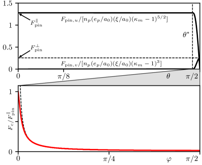
Figure 9: Top: scaled pinning force densities $F_{\mathrm{pin},u}$ and $F_{\mathrm{pin},v}$ versus impact angle $\theta$; we have used the same parameters as in Fig. 6. The longitudinal (along $u$) force $F_{\mathrm{pin},u}$ remains constant and equal to $F_{\mathrm{pin}}^{\parallel}$ for all angles $|\theta|<\theta^{\ast}$, while the transverse (along $v$) component $F_{\mathrm{pin},v}$ vanishes in this regime. The longitudinal force drops and vanishes over the narrow interval $\theta^{\ast}<|\theta|<\pi/2$, while the transverse force $F_{\mathrm{pin},v}$ increases up to $F_{\mathrm{pin}}^{\perp}$. Bottom: critical force density $F_{c}$ (directed along the Lorentz force $\mathbf{F}_{\rm\scriptscriptstyle L}=\mathbf{j}\wedge\mathbf{B}/c$) versus angle $\varphi$ of the Lorentz force; the dashed line shows the upper bound $F_{c}<F_{\mathrm{pin}}^{\perp}/\sin(\varphi)$.

III.7.3 Anisotropic critical force density $\mathbf{F}_{c}$

When the vortex system is subjected to a current density $\mathbf{j}$, the associated Lorentz force $\mathbf{F}_{\rm\scriptscriptstyle L}(\varphi)=\mathbf{j}\wedge\mathbf{B}/c$ directed along $\varphi$ pushes the vortices across the defects. When $\mathbf{F}_{\rm\scriptscriptstyle L}$ is directed along $u$, we have $\mathbf{F}_{\mathrm{pin}}=[F_{\mathrm{pin}}^{\parallel},0]$ and the vortex system gets immobilized at force densities $F_{\rm\scriptscriptstyle L}<F_{c}=F_{\mathrm{pin}}^{\parallel}$ (or associated current densities $\mathbf{j}_{c}$). When $\mathbf{F}_{\rm\scriptscriptstyle L}$ is directed away from $u$, the driving component along $v$ has to be compensated by a finite pinning force $F_{\mathrm{pin},v}$ that appears only for angles $\theta^{\ast}<\theta<\pi/2$. Hence, the angles of force and motion, $\varphi$ associated with the Lorentz force $\mathbf{F}_{\rm\scriptscriptstyle L}(\varphi)$ and $\theta$ providing the direction of the pinning force $\mathbf{F}_{\mathrm{pin}}(\theta)$, are different. We find them, along with the critical force density $\mathbf{F}_{c}(\varphi)$, by solving the dynamical force equation (17) at vanishing velocity $\mathbf{v}=0$,

$$\mathbf{F}_{c}(\varphi)=\mathbf{F}_{\mathrm{pin}}(\theta)$$ (89)

resulting in a critical force density

$$F_{c}(\varphi)=\sqrt{F_{\mathrm{pin},u}^{2}(\theta)+F_{\mathrm{pin},v}^{2}(\theta)}$$ (90)

with angles $\varphi$ and $\theta$ related via

$$\tan\varphi=\frac{F_{\mathrm{pin},u}(\theta)}{F_{\mathrm{pin},v}(\theta)}.$$ (91)

Since $F_{\mathrm{pin},u}(\theta<\theta^{\ast})=0$, the entire interval $\theta<\theta^{\ast}$ is compressed to $\varphi=0$ and it is the narrow regime $\theta^{\ast}<\theta<\pi/2$ that determines the angular characteristic of the critical force density $F_{c}(\varphi)$. The critical force density $F_{c}(\varphi)$ is peaked at $\varphi=0$ as shown in Fig. 9 (with a correspondingly sharp peak in $j_{c}$ at right angles). Combing Eqs. (90) and (91), we can derive a simple expression bounding the function $F_{c}(\varphi)$,

$$F_{c}(\varphi)=F_{\mathrm{pin},v}(\theta)\sqrt{1+\cot^{2}(\varphi)}\leq\frac{F_{\mathrm{pin}}^{\perp}}{\sin(\varphi)},$$ (92)

that traces $F_{c}(\varphi)$ over a wide angular region, see the dashed line in Fig. 9. At small values of $\varphi$ we cannot ignore the angular dependence in $F_{\mathrm{pin},v}(\theta)$ any more that finally cuts off the divergence $\propto 1/\sin(\varphi)$ at the value $F_{c}(\varphi\to 0)\to F_{\mathrm{pin}}^{\parallel}$.

III.7.4 Isotropized pinning force density $F_{\mathrm{pin}}$

In a last step, we assume an ensemble of equal anisotropic defects that are uniformly distributed in space and randomly oriented. In this situation, we have to perform an additional average over the instability directions $\hat{\mathbf{u}}_{i}$ associated with the different defects $i=1,\dots N$. Neglecting the modification of $\mathbf{F}_{\mathrm{pin}}(\theta)$ away from $[F_{\mathrm{pin}}^{\parallel},0]$ in the small angular regions $\theta^{\ast}<|\theta|<\pi/2$, we find that the force along any direction $\hat{\mathbf{R}}$ has the magnitude

$$F_{\mathrm{pin}} \approx \frac{1}{N}\sum_{i=1}^{N}|(F_{\mathrm{pin}}^{\parallel}\hat{\mathbf{u}}_{i})\cdot\hat{\mathbf{R}}|$$

$$\approx F^{\parallel}_{\mathrm{pin}}\int_{-\pi/2}^{\pi/2}\frac{\mathrm{d}\theta}{\pi}\,\cos\theta=\frac{2}{\pi}F_{\mathrm{pin}}^{\parallel}.$$

As a result of the averaging over the angular directions, the pinning force density is now effectively isotropic and directed against the velocity $\mathbf{v}$ of the vortex motion.

IV Uniaxial defect

In Sec. III, we have analyzed the onset of strong pinning for an arbitrary potential and have determined the shape of the unstable and bistable domains $\mathcal{U}_{\tilde{\bf R}}$ and $\mathcal{B}_{\bar{\bf R}}$—with their elliptic and crescent forms, they look quite different from their ring-shaped counterparts for the isotropic defect in Figs. 5(c) and (d). In this section, we discuss the situation for a weakly anisotropic defect with a small uniaxial deformation quantified by the small parameter $\epsilon$ in order to understand how our previous findings, the results for the isotropic defect and those describing the strong-pinning onset, relate to one another.

Our weakly deformed defect is described by equipotential lines that are nearly circular but slightly elongated along $y$, implying that pinning is strongest in the $x$-direction. We will find that the unstable (bistable) domain $\mathcal{U}_{\tilde{\bf R}}$ ($\mathcal{B}_{\bar{\bf R}}$) for the uniaxially anisotropic defect starts out with two ellipses (crescents) on the $x$-axis as $\kappa_{m}$ crosses unity. With increasing pinning strength, i.e., $\kappa_{m}$, these ellipses (crescents) grow and deform to follow the equipotential lines, with the end-points approaching one another until they merge on the $\pm y$-axis. These merger points, we denote them as $\tilde{\bf R}_{s}$ and $\bar{\bf R}_{s}$, define a second class of important points (besides the onset points $\tilde{\bf R}_{m}$ and $\bar{\bf R}_{m}$) in the buildup of the strong pinning landscape: while the onset points $\tilde{\bf R}_{m}$ are defined as minima of the Hessian determinant $D(\tilde{\bf R})$, the merger points $\tilde{\bf R}_{s}$ turn out to be associated with saddle points of $D(\tilde{\bf R})$. Pushing across the merger of the deformed ellipses (crescents) by further increasing the Labusch parameter $\kappa_{m}$, the unstable (bistable) domains $\mathcal{U}_{\tilde{\bf R}}$ ($\mathcal{B}_{\bar{\bf R}}$) undergo a change in topology, from two separated areas to a ring-like geometry as it appears for the isotropic defect, see Figs. 5(c) and (d), thus explaining the interrelation of our results for isotropic and anisotropic defects.

With this analysis, we thus show how the strong pinning landscape for the weakly uniaxial defect will finally assume the shape and topology of the isotropic defect as the pinning strength $\kappa_{m}$ overcomes the anisotropy $\epsilon$. Second, this discussion will introduce the merger points $\tilde{\bf R}_{s}$ as a second type of characteristic points of strong pinning landscapes that we will further study in section V.1 using a Landau-type expansion as done in section III.1 above; we will find that the geometry of the merger points $\tilde{\bf R}_{s}$ is associated with hyperbolas, as that of the onset points was associated with ellipses.

Our uniaxially anisotropic defect is described by the stretched (along the $y$-axis) Lorentzian

$$e_{p}(\tilde{x},\tilde{y})=-e_{p}\left(1+\frac{\tilde{x}^{2}}{2\xi^{2}}+\frac{\tilde{y}^{2}}{2\xi^{2}\left(1+\epsilon\right)^{2}}\right)^{-1},$$ (94)

with equipotential lines described by ellipses

$$\frac{\tilde{x}^{2}}{\xi^{2}}+\frac{\tilde{y}^{2}}{\xi^{2}\left(1+\epsilon\right)^{2}}=\text{const},$$ (95)

and the small parameter $0<\epsilon\ll 1$ quantifying the degree of anisotropy. At fixed radius $\tilde{R}^{2}=\tilde{x}^{2}+\tilde{y}^{2}$, the potential (94) assumes maxima in energy and in negative curvature on the $x-$axis, and corresponding minima on the $y-$axis. Along both axes, the pinning force is directed radially towards the origin and the Labusch criterion (34) for strong pinning is determined solely by the curvature along the radial direction. At the onset of strong pinning, the unstable and bistable domains then first emerge along the $x-$axis at the points $\tilde{\bf R}_{m}=(\pm\sqrt{2}\xi,0)$ and $\bar{\bf R}_{m}=(\pm 2\sqrt{2}\xi,0)$ when

$$\kappa_{m}=\frac{e_{p}}{4\bar{C}\xi^{2}}=1.$$ (96)

Upon increasing the pinning strength $\kappa_{m}$, e.g., via softening of the vortex lattice as described by a decrease in $\bar{C}$, the unstable and bistable domains $\mathcal{U}_{\tilde{\bf R}}$ and $\mathcal{B}_{\bar{\bf R}}$ expand away from these points, and eventually merge along the $y-$axis at $\tilde{\bf R}_{s}=(0,\pm\sqrt{2}\xi(1+\epsilon))$, $\bar{\bf R}_{s}=(0,\pm 2\sqrt{2}\xi(1+\epsilon))$ when

$$\kappa_{s}=\frac{e_{p}}{4\bar{C}\xi^{2}(1+\epsilon)^{2}}=\frac{\kappa_{m}}{(1+\epsilon)^{2}}=1,$$ (97)

i.e., for $\kappa_{m}=(1+\epsilon)^{2}$. The evolution of the strong pinning landscape from onset to merging takes place in the interval $\kappa_{m}\in[1,(1+\epsilon)^{2}]$; pushing $\kappa_{m}$ beyond this interval, we will analyze the change in topology and appearance of non-simply connected unstable and bistable domains after the merging.

The quantity determining the shape of the unstable domain $\mathcal{U}_{\tilde{\bf R}}$ is the Hessian determinant $D(\tilde{\bf R})$ of the total vortex energy $e_{\mathrm{pin}}(\tilde{\bf R};\bar{\bf R})$, see Eqs. (36) and (1), respectively. At onset, the minimum of $D(\tilde{\bf R})$ touches zero for the first time; with increasing $\kappa_{m}$, this minimum drops below zero and the condition $D(\tilde{\bf R})=0$ determines the unstable ellipse that expands in $\tilde{\bf R}$-space. Viewing the function $D(\tilde{\bf R})$ as a height function of a landscape in the $\tilde{\bf R}$ plane, this corresponds to filling this landscape, e.g., with water, up to the height level $D=0$ with the resulting lake representing the unstable domain. In the present uniaxially symmetric case, a pair of unstable ellipses grow simultaneously, bend around the equipotential line near the radius $\sim\sqrt{2}\xi$ and finally touch upon merging on the $y$-axis. In our geometric interpretation, this corresponds to the merging of the two (water-filled) valleys that happens in a saddle-point of the function $D(\tilde{\bf R})$ at the height $D=0$. Hence, the merger point $\tilde{\bf R}_{s}$ correspond to saddles in $D(\tilde{\bf R})$ with

$$D(\tilde{\bf R}_{s})=0,\quad\mathbf{\nabla}_{\tilde{\bf R}}\,D(\mathbf{R})\big{|}_{\tilde{\bf R}_{s}}=0,$$ (98)

and

$$\mathrm{det}\bigl{[}\mathrm{Hess}\bigl{[}D(\tilde{\bf R})\bigr{]}\bigr{]}\big{|}_{\tilde{\bf R}_{s}}<0,$$ (99)

cf. Eq. (44).

In our calculation of $D(\tilde{\bf R})$, we exploit that the Hessian in (36) does not depend on the asymptotic position $\bar{\bf R}$ and we can set it to zero,

$$D(\tilde{\bf R}) =\det\{\mathrm{Hess}[\bar{C}\tilde{R}^{2}/2+e_{p}^{\scriptscriptstyle(i)}(\tilde{R})+\delta e_{p}(\tilde{\bf R})]\bigr{\}},$$ (100)

where we have split off the anisotropic correction $\delta e_{p}(\tilde{\bf R})=e_{p}(\tilde{\bf R})-e_{p}^{\scriptscriptstyle(i)}(\tilde{R})$ away from the isotropic potential $e_{p}^{\scriptscriptstyle(i)}(\tilde{R})$ with $\epsilon=0$. In the following, we perform a perturbative analysis around the isotropic limit valid in the limit of weak anisotropy $\epsilon\ll 1$; this motivates our use of polar (tip) coordinates $\tilde{R}$ and $\tilde{\phi}$.

The isotropic contribution $\mathrm{H}^{\scriptscriptstyle(i)}$ to the Hessian matrix $\mathrm{H}$ is diagonal with components

$$\mathrm{H}^{\scriptscriptstyle(i)}_{\tilde{R}\tilde{R}}(\tilde{R}) \equiv\partial_{\tilde{R}}^{2}[\bar{C}\tilde{R}^{2}/2+e_{p}^{\scriptscriptstyle(i)}(\tilde{R})]$$

$$=\bar{C}+\partial_{\tilde{R}}^{2}e_{p}^{\scriptscriptstyle(i)}(\tilde{R})$$ (101)

and

$$\mathrm{H}^{\scriptscriptstyle(i)}_{\tilde{\phi}\tilde{\phi}}(\tilde{R}) \equiv(\tilde{R}^{-2}\partial^{2}_{\tilde{\phi}\tilde{\phi}}+\tilde{R}^{-1}\partial_{\tilde{R}})[\bar{C}\tilde{R}^{2}/2+e_{p}^{\scriptscriptstyle(i)}(\tilde{R})]$$

$$=\bar{C}-f_{p}^{\scriptscriptstyle(i)}(\tilde{R})/\tilde{R}.$$ (102)

The radial component $\mathrm{H}^{\scriptscriptstyle(i)}_{\tilde{R}\tilde{R}}\propto(\kappa_{m}-1)$ vanishes at onset, while $\mathrm{H}^{\scriptscriptstyle(i)}_{\tilde{\phi}\tilde{\phi}}$ remains finite, positive, and approximately constant.

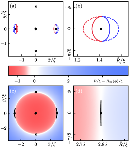
Figure 10: Unstable and bistable domains close to the onset of strong pinning for a uniaxial defect (94) centered at the origin, with $\epsilon=0.1$ and $\kappa_{m}-1=0.01$. The pinning potential is steepest at angles $\tilde{\phi}=0,\,\pi$ and least steep at $\tilde{\phi}=\pm\pi/2$, hence strong pinning is realized first in a small interval around $\tilde{\phi}=0,\,\pi$ (solid black dots) where $\kappa_{m}(\tilde{\phi})\geq 1$. (a) The unstable domain $\mathcal{U}_{\tilde{\bf R}}$ in tip space is bounded by red/blue solid lines (jump lines $\mathcal{J}_{\mathrm{\tilde{\bf R}}}$, see Eq. (108)); dashed lines mark the associated landing lines $\mathcal{L}_{\mathrm{\tilde{\bf R}}}$, see (114). (b) Focus on the unstable domain near $\tilde{\phi}=0$ in polar coordinates $\tilde{R}$ and $\tilde{\phi}$. The jumping (solid) and landing (dashed) lines have the approximate shape of ellipses, see Eq. (111), in agreement with our analysis of Sec. III.2. (c) The bistable domain $\mathcal{B}_{\bar{\bf R}}$ in asymptotic space involves symmetric crescents centered at $\bar{\phi}=0,\,\pi$ and a narrow width $\propto(\kappa_{m}(\bar{\phi})-1)^{3/2}$, see Eq. (112), in agreement with the analysis of Sec. III.3. (d) Focus on the bistable domain at $\bar{\phi}=0$ in polar coordinates $\bar{R}$ and $\bar{\phi}$. Red/blue colors indicate different vortex configurations as quantified through the order parameter $\tilde{R}-\tilde{R}_{m}(\tilde{\phi})$.

The anisotropic component $\delta e_{p}(\tilde{\bf R})$ introduces corrections $\propto\epsilon$; these significantly modify the radial entry of the full Hessian while leaving its azimutal component $\mathrm{H}_{\tilde{\phi}\tilde{\phi}}$ approximately unchanged; the off-diagonal entries of the full Hessian scale as $\epsilon$ and hence contribute in second order of $\epsilon$ to $D(\tilde{\bf R})$. As a result, the sign change in the determinant

$$D(\tilde{\bf R})\approx\mathrm{H}_{\tilde{R}\tilde{R}}(\tilde{\bf R})\mathrm{H}_{\tilde{\phi}\tilde{\phi}}(\tilde{R})+\mathcal{O}\left(\epsilon^{2}\right),$$ (103)

is determined by

$$\mathrm{H}_{\tilde{R}\tilde{R}}(\tilde{\bf R})=\mathrm{H}^{\scriptscriptstyle(i)}_{\tilde{R}\tilde{R}}(\tilde{R})+\partial^{2}_{\tilde{R}}\delta e_{p}(\tilde{\bf R})$$ (104)

for radii close to $\tilde{R}_{m}$ with $\delta\tilde{R}=\tilde{R}-\tilde{R}_{m}\approx\mathcal{O}(\sqrt{\kappa_{m}-1})$. We expand the potential (94) around the isotropic part $e_{p}^{\scriptscriptstyle(i)}(\tilde{R})$,

$$\delta e_{p}(\tilde{\bf R})\approx-\epsilon\,[\partial_{\tilde{R}}e_{p}^{\scriptscriptstyle(i)}(\tilde{R})]\tilde{R}\sin^{2}\tilde{\phi},$$ (105)

and additionally expand both $e_{p}^{\scriptscriptstyle(i)}(\tilde{R})$ and $\delta e_{p}(\tilde{\bf R})$ around $\tilde{R}_{m}$, keeping terms $\propto\epsilon\,\sqrt{(\kappa_{m}-1)}$. The radial entry of the anisotropic Hessian matrix then assumes the form

$$\mathrm{H}_{\tilde{R}\tilde{R}}(\tilde{\bf R})\approx\bar{C}\,[1-\kappa_{m}(\tilde{\phi})]\\ +\gamma\,[\delta\tilde{R}^{2}/2-\epsilon\,\sin^{2}{\tilde{\phi}}\,\tilde{R}_{m}\delta\tilde{R}]$$ (106)

with $\gamma=\partial^{4}_{\tilde{R}}e_{p}^{\scriptscriptstyle(i)}(\tilde{R})|_{\tilde{R}_{m}}$ and the angle-dependent Labusch parameter

$$\kappa_{m}(\tilde{\phi})\equiv\frac{\max_{\tilde{R}}[-\partial_{\tilde{R}}^{2}e_{p}(\tilde{R},\tilde{\phi})|_{\tilde{\phi}}]}{\bar{C}}=\kappa_{m}-2\epsilon\sin^{2}\tilde{\phi}.$$ (107)

The edges of the unstable region $\mathcal{U}_{\tilde{\bf R}}$ then can be obtained by imposing the condition $\mathrm{H}_{\tilde{R}\tilde{R}}(\tilde{\bf R})=0$ and the solution to the corresponding quadratic equation define the jump positions $\tilde{R}_{\mathrm{jp}}(\tilde{\phi})$ (or boundaries $\partial\mathcal{U}_{\tilde{\bf R}}$)

$$\tilde{R}_{\mathrm{jp}}(\tilde{\phi})\approx\tilde{R}_{m}(\tilde{\phi})\pm\delta\tilde{R}(\tilde{\phi}).$$ (108)

These are centered around the (‘large’) ellipse defined by

$$\tilde{R}_{m}(\tilde{\phi})=\tilde{R}_{m}(1+\epsilon\sin^{2}\tilde{\phi})$$ (109)

and separated by (cf. Eq. (20))

$$2\,\delta\tilde{R}(\tilde{\phi})=\sqrt{\frac{8\bar{C}}{\gamma}(\kappa_{m}(\tilde{\phi})-1)}$$ (110)

along the radius. Making use of the form (107) of $\kappa_{m}(\tilde{\phi})$ and assuming a small value of $\kappa_{m}>1$ near onset, we obtain the jump line in the form of a (‘small’) ellipse centered at $[\pm\tilde{R}_{m},0]$,

$$\gamma\,\delta\tilde{R}^{2}+\epsilon\bar{C}\,\tilde{\phi}^{2}=\bar{C}(\kappa_{m}-1).$$ (111)

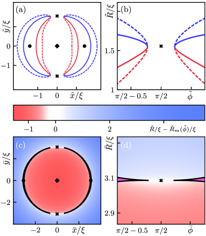
Figure 11: Unstable and bistable domains before merging for a uniaxial defect (94) centered at the origin, with $\epsilon=0.1$ and $1-\kappa_{s}\approx 0.01$. Strong pinning is realized everywhere but in a small interval around $\tilde{\phi}=\pm\pi/2$ where $\kappa_{m}(\tilde{\phi})<1$. (a) The unstable domain $\mathcal{U}_{\tilde{\bf R}}$ in the tip plane is bounded by the solid red/blue jump lines $\mathcal{J}_{\mathrm{\tilde{\bf R}}}$, see Eq. (108) and involves two strongly bent ellipses originating from angles $\tilde{\phi}=0,\,\pi$ (black dots) and approaching one another close to $\tilde{\phi}=\pm\pi/2$ (black crosses); red/blue dashed lines are landing points as given by Eqs. (114). (b) Focus (in polar coordinates $\tilde{R},\,\tilde{\phi}$) on the tips of the unstable domain near $\tilde{\phi}=\pi/2$. (c) The bistable domain $\mathcal{B}_{\bar{\bf R}}$ in the asymptotic space consists of thin symmetric crescents (colored in magenta) originating from $\bar{\phi}=0,\,\pi$, with the delimiting black solid lines given by Eq. (112). (d) Focus on the cusps of the bistable domain close to $\bar{\phi}=\pi/2$ in polar coordinates $\bar{R},\,\bar{\phi}$. Red/blue colors indicate different vortex configurations as quantified through the order parameter $\tilde{R}-\tilde{R}_{m}(\bar{\phi})$.

Hence, we find that the anisotropic results are obtained from the isotropic ones by replacing the circle $\tilde{R}_{m}$ by the ellipse $\tilde{\bf R}_{m}(\tilde{\phi})$ and substituting $\kappa\to\kappa_{m}(\tilde{\phi})$ in the width (20), see Figs. 10(a) and (b) evaluated for small values $\kappa_{m}-1=0.01$ and $\epsilon=0.1$.

Analogously, the boundaries of the bistable domain $\mathcal{B}_{\bar{\bf R}}$ can be found by applying the same substitutions to the result (25), see Figs. 10(c) and (d),

$$\bar{R}(\bar{\phi})\approx\bar{R}_{m}(\bar{\phi})\pm\delta\bar{R}(\bar{\phi})$$ (112)

with $\bar{R}_{m}(\bar{\phi})=\bar{R}_{m}(1+\epsilon\sin^{2}\bar{\phi})$ and the width

$$2\,\delta\bar{R}(\bar{\phi})=\frac{2}{3}\sqrt{\frac{8\bar{C}}{\gamma}}(\kappa_{m}(\tilde{\phi})-1)^{3/2}.$$ (113)

The landing line $\mathcal{L}_{\tilde{\bf R}}$ is given by (see Eq. (23) and note that the jump point is shifted by $\tilde{u}_{\mathrm{jp}}$ away from $\tilde{x}_{m}$, see Eq. (19))

$$\tilde{R}_{\mathrm{lp}}(\tilde{\phi})\approx\tilde{R}_{m}(\tilde{\phi})\mp 2\,\delta\tilde{R}(\tilde{\phi}).$$ (114)

An additional complication is the finite angular extension of the unstable and bistable domains $\mathcal{U}_{\tilde{\bf R}}$ and $\mathcal{B}_{\bar{\bf R}}$; these are limited by the condition $\kappa_{m}(\phi_{\max})=1$, providing us with the constraint

$$\tilde{\phi}_{\max}=\bar{\phi}_{\max}\approx\pm\sqrt{\frac{\kappa_{m}-1}{2\epsilon}}$$ (115)

near the strong pinning onset with $(\kappa_{m}-1)\ll\epsilon$. The resulting domains $\mathcal{U}_{\tilde{\bf R}}$ have characteristic extensions of scale $\propto\sqrt{\kappa_{m}-1}$, see Fig. 10.

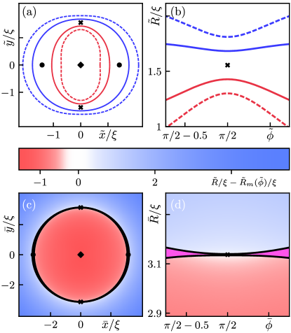
Figure 12: Unstable and bistable domains for a uniaxial defect (94) after merging, with $\epsilon=0.1$ and $\kappa_{s}-1\approx 0.01$. (a) The unstable domain $\mathcal{U}_{\tilde{\bf R}}$ in tip plane is enclosed between the jump lines $\mathcal{J}_{\mathrm{\tilde{\bf R}}}$ (solid red/blue, see Eq. (108)) and takes the shape of a deformed ring with a wider (narrower) width at strongest (weakest) pinning near the solid dots (crosses). Red/blue dashed lines mark the landing positions $\mathcal{L}_{\mathrm{\tilde{\bf R}}}$ of the vortex tips and are given by Eq. (114). (b) Focus on the narrowing in the unstable domain close to the merger points (crosses) at $\tilde{\phi}=\pi/2$ in the polar coordinates $\tilde{R},\,\tilde{\phi}$. (c) The bistable domain $\mathcal{B}_{\bar{\bf R}}$ in asymptotic space is a narrow ring (colored in magenta) thicker (thinner) at points of strongest (weakest) pinning near $\bar{\phi}=0,\ \pi$ ($\bar{\phi}=\pm\pi/2$); black lines correspond to Eq. (112). (d) Focus on the constriction in the bistable domain close to $\bar{\phi}=\pi/2$ in polar coordinates $\bar{R},\,\bar{\phi}$. Red/blue colors indicate different vortex configurations as quantified through the order parameter $\tilde{R}-\tilde{R}_{m}(\bar{\phi})$.

Close to merging (marked by crosses in the figure) at $\phi=\pm\pi/2$, we define the deviation $\delta\phi=\pi/2-\phi$ with $\delta\phi\ll 1$, and imposing the condition $\kappa_{m}(\phi_{\max})=1$, we find

$$\delta\tilde{\phi}_{\max}=\delta\bar{\phi}_{\max}\approx\sqrt{1-\frac{\kappa_{m}-1}{2\epsilon}}\approx\sqrt{\frac{1-\kappa_{s}}{2\epsilon}}.$$ (116)

The corresponding geometries of $\mathcal{U}_{\tilde{\bf R}}$ and $\mathcal{B}_{\bar{\bf R}}$ are shown in Fig. 11 for $1-\kappa_{s}\approx 0.01$ and $\epsilon=0.1$. Finally, $\delta\tilde{\phi}_{\max}$ vanishes at merging for $\kappa_{s}=1$ (or $\kappa_{m}-1\approx 2\epsilon$), in agreement, to order $\epsilon$, with the exact result (97).

Pushing the Labusch parameter beyond the merger with $\kappa_{s}>1$ or $\kappa_{m}>(1+\epsilon)^{2}\approx 1+2\epsilon$, the unstable and bistable regimes $\mathcal{U}_{\tilde{\bf R}}$ and $\mathcal{B}_{\bar{\bf R}}$ change their topology: they develop a (non-simply connected) ring-like geometry with separated inner and outer edges that are a finite distance apart in the radial direction at all angles $\tilde{\phi}$ and $\bar{\phi}$. The situation after the merger is shown in Fig. 12 for $\kappa_{s}-1\approx 0.01$ and $\epsilon=0.1$, with the merging points $\tilde{\bf R}_{s}$ and $\bar{\bf R}_{s}$ marked by crosses.

The merging of the unstable domains at the saddle point $\tilde{\bf R}_{s}$ is a general feature of irregular pinning potentials. In the next section, we will analyze the behavior of the unstable domains close to a saddle point $\tilde{\bf R}_{s}$ of the Hessian determinant $D(\tilde{\bf R})$ and obtain a universal description of their geometry close to this point. We will see that the geometry associated with this merger is of a hyperbolic type described by $\gamma\tilde{u}^{2}+\delta\tilde{v}^{2}=2\bar{C}(\kappa_{s}-1)$, $\gamma>0$ and $\delta<0$ (assuming no skew). The change in topology then is driven by the sign change in $\kappa_{s}-1$: before merging, $\kappa_{s}<1$, the hyperbola is open along the unstable (radial) direction $\tilde{u}$, thus separating the two unstable regions, while after merging, $\kappa_{s}>1$, the hyperbola is open along the transverse direction $\tilde{v}$, with the ensuing passage defining the single, non-simply connected, ring-like unstable region.

V Merger points

The merging of unstable and bistable domains is a general feature of irregular pinning potentials that is relevant beyond the simple example of a weakly anisotropic uniaxial defect discussed above. Indeed, while the exact geometries of $\mathcal{U}_{\tilde{\bf R}}$ and $\mathcal{B}_{\bar{\bf R}}$ depend on the precise shape of the pinning potential, their behavior close to merging is universal. Below, we will study this universal behavior by generalizing the expansions of Sec. III to saddle points $\tilde{\bf R}_{s}$ of the determinant $D(\tilde{\bf R})$. As with the onset of strong pinning, the merger of two domains induces a change in topology in the unstable and bistable domains; we will discuss these topological aspects of onsets and mergers in Secs. V.4 and VI below.

V.1 Expansion near merger

Following the strategy of Sec. III, we expand the energy functional around a saddle point $\tilde{\bf R}_{s}$ of the determinant $D(\tilde{\bf R})$ in order to obtain closed expressions for the unstable and bistable domains at merging. In doing so, we again define local coordinate systems $(\tilde{u},\tilde{v})$ and $(\bar{u},\bar{v})$ in tip- and asymptotic space centered at $\tilde{\bf R}_{s}$ and $\bar{\bf R}_{s}$, where the latter is associated with $\tilde{\bf R}_{s}$ through the force balance equation (38) in the original laboratory system. Furthermore, we fix our axes such that $D(\tilde{\bf R}_{s})$ is a local maximum along the (unstable) $u$- and a local minimum along the (stable) $v$-direction of the saddle; the mixed term $\propto\tilde{u}\tilde{v}$ is absent from the expansion (as the Hessian matrix is symmetric). Furthermore, the vanishing slopes at the saddle point, see (98), imply the absence of terms $\propto\tilde{u}^{3}$ and $\propto\tilde{u}^{2}\tilde{v}$ in the expansion and dropping higher-order terms (corresponding to double-primed terms in (40)), we arrive to the expression

$$e_{\mathrm{pin}}(\tilde{\bf R};\bar{\bf R})=\frac{\bar{C}}{2}(1-\kappa_{s})\,\tilde{u}^{2}+\frac{\bar{C}+\lambda_{+,s}}{2}\,\tilde{v}^{2}+\frac{a_{s}}{2}\,\tilde{u}\tilde{v}^{2}$$

$$\quad+\frac{\alpha_{s}}{4}\,\tilde{u}^{2}\tilde{v}^{2}+\frac{\beta_{s}}{6}\,\tilde{u}^{3}\tilde{v}+\frac{\gamma_{s}}{24}\,\tilde{u}^{4}-\bar{C}\bar{u}\tilde{u}-\bar{C}\bar{v}\tilde{v},$$ (117)

with $\kappa_{s}\equiv-\lambda_{-}(\tilde{\bf R}_{s})/\bar{C},\ \lambda_{+,s}\equiv\lambda_{+}(\tilde{\bf R}_{s})$ and the remaining coefficients defined in analogy to Eq. (III.2.1).

The most important term in the expansion (V.1) is the curvature term $\bar{C}(1-\kappa_{s})\,\tilde{u}^{2}/2$ along the unstable direction $u$. As before in Sec. III.2, see Eq. (III.2.1), the coefficient $(1-\kappa_{s})$ changes sign at some value of the pinning strength and will serve as the small parameter in our considerations. The higher-order terms in the expansion (V.1) are constrained by the saddle condition (99), implying that (cf. (48) and (50))

$$\gamma_{s}\delta_{s}-\beta_{s}^{2}<0$$ (118)

with

$$\delta_{s}\equiv\alpha_{s}-\frac{2a_{s}^{2}}{\bar{C}+\lambda_{+,s}}$$ (119)

(for the saddle point there is no condition on the trace of the Hessian). The mapping of the two-dimensional pinning energy (V.1) to an effective one-dimensional Landau theory (178) of the van der Waals kind is discussed in Appendix A.2, both before and after merging.

V.2 Unstable domain $\mathcal{U}_{\tilde{\bf R}}$

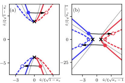
Figure 13: Jump lines $\mathcal{J}_{\mathrm{\tilde{\bf R}}}$ (solid red/blue) and landing lines $\mathcal{L}_{\mathrm{\tilde{\bf R}}}$ (dashed red/blue) in tip space $\tilde{\bf R}$ (in units of $\xi$), with the hyperbola $\mathcal{J}_{\mathrm{\tilde{\bf R}}}$ defining the edge $\partial\mathcal{U}_{\tilde{\bf R}}$ of the unstable domain $\mathcal{U}_{\tilde{\bf R}}$, before (a) and after (b) merging, for $1-\kappa_{s}=\pm 0.01$. Parameters are $\lambda_{-,s}=-0.25\,e_{p}/\xi^{2},\lambda_{+,s}=0$, and $a_{s}\approx 0.035\,e_{p}/\xi^{3}$, $\alpha_{s}=-0.025\,e_{p}/\xi^{4}$, $\beta_{s}=0$, $\gamma_{s}\approx 0.68\,e_{p}/\xi^{4}$. A finite skew parameter $\beta_{s}=0.025e_{p}/\xi^{4}$ tilts the hyperbola away from the axes (dotted curves). Crosses correspond to the vertices (125) and (129) of the hyperbola before and after merging. Pairs of solid and open circles connected via long arrows are examples of pairs of jumping- and landing tip positions. After merging, see (b), the unstable domain $\mathcal{U}_{\tilde{\bf R}}$ is connected along the $\tilde{v}$-axis, dividing the tip coordinate plane into two separate regions. The jumping and landing hyperbolas coincide at their vertices before merging, see (a), but not thereafter, see (b), where the jumping and landing hyperbolas are separated (vertices on $\mathcal{L}_{\mathrm{\tilde{\bf R}}}$ are marked with open red/blue stars) and no contact point is present. Note the rotation by 90 degrees of the unstable direction with respect to Figs. 11(b) and 12(b).

V.2.1 Jump line $\mathcal{J}_{\mathrm{\tilde{\bf R}}}$

The boundary of the unstable domain $\mathcal{U}_{\tilde{\bf R}}$ is determined by the jump condition $D(\tilde{\bf R}_{s,\mathrm{jp}})=0$. Making use of the expansion (V.1) and keeping only terms quadratic in $\tilde{u},\tilde{v}$, the edges $\delta\tilde{\bf R}_{s,\mathrm{jp}}=(\tilde{u}_{s,\mathrm{jp}},\tilde{v}_{s,\mathrm{jp}})$ of $\mathcal{U}_{\tilde{\bf R}}$ (measured relative to $\tilde{\bf R}_{s}$) are given by the solutions of the quadratic form (cf. (53))

$$[\gamma_{s}\,\tilde{u}^{2}+2\beta_{s}\,\tilde{u}\tilde{v}+\delta_{s}\,\tilde{v}^{2}]_{\tilde{\bf R}_{s,\mathrm{jp}}}=2\bar{C}(\kappa_{s}-1).$$ (120)

Equation (120) describes a hyperbola (centered at $\tilde{\bf R}_{s}$) as its associated determinant is negative, see Eq. (118). Again, (120) can be cast in the form of a matrix equation

$$\delta\tilde{\bf R}_{s,\mathrm{jp}}^{T}M_{s,\mathrm{jp}}\delta\tilde{\bf R}_{s,\mathrm{jp}}=\bar{C}(\kappa_{s}-1),$$ (121)

with $M_{s,\mathrm{jp}}$ given by

$$M_{s,\mathrm{jp}} =\begin{bmatrix}\gamma_{s}/2&~{}~{}~{}\beta_{s}/2\\ \beta_{s}/2&~{}~{}~{}\delta_{s}/2\end{bmatrix}$$ (122)

with $\det M_{s,\mathrm{jp}}=(\gamma_{s}\delta_{s}-\beta_{s}^{2})/4<0$. As shown in Fig. 13, the geometry of the unstable domain $\mathcal{U}_{\tilde{\bf R}}$ changes drastically when $1-\kappa_{s}$ changes sign. Before merging, i.e., for $1-\kappa_{s}>0$, the unstable domain (top and bottom regions in Fig. 13(a)) is disconnected along the stable $v$-direction and the two red/blue branches of the hyperbola (120) describe the tips of $\mathcal{U}_{\tilde{\bf R}}$. When $\kappa_{s}$ goes to unity, the tips of the unstable domain merge at the saddle point $\tilde{\bf R}_{s}$. After merging, the unstable domain extends continuously from the top to the bottom in Fig. 13(b) with a finite width along the unstable $u$-direction, similarly to the isotropic case shown in Fig. 5(c). Correspondingly, the two (red and blue) branches of the hyperbola (120) now describe the edges of $\mathcal{U}_{\tilde{\bf R}}$.

Solving the quadratic equation (120) before merging, i.e., $1-\kappa_{s}>0$, we find solutions $\tilde{u}_{s,\mathrm{jp}}(\tilde{v})$ away from a gap along the stable $v$-direction,

$$\tilde{u}_{s,\mathrm{jp}}(|\tilde{v}|\geq\tilde{v}_{s,c})=-\frac{1}{\gamma_{s}}\Bigl{[}\beta_{s}\tilde{v}\\ \pm\sqrt{2\gamma_{s}\bar{C}(\kappa_{s}-1)-(\gamma_{s}\delta_{s}-\beta_{s}^{2})\tilde{v}^{2}}\Bigr{]},$$ (123)

i.e., Eq. (123) has real solutions in the (unbounded) interval $|\tilde{v}|\geq\tilde{v}_{s,c}$, with

$$\tilde{v}_{s,c}=\sqrt{2\gamma_{s}\bar{C}(1-\kappa_{s})/|\gamma_{s}\delta_{s}-\beta_{s}^{2}|}.$$ (124)

For the uniaxial defect (94) before merging, this gap corresponds to a splitting of $\mathcal{U}_{\tilde{\bf R}}$ along the stable angular direction, producing two separated domains as shown in Fig. 11(a). The coordinates $\left(\tilde{u}_{s,\mathrm{jp}}(\pm\tilde{v}_{s,c}),\pm\tilde{v}_{s,c}\right)$ give the positions of the vertices $\delta\tilde{\bf R}^{<}_{s,c,\pm}$ (relative to $\tilde{\bf R}_{s}$) of the hyperbola before merging,

$$\delta\tilde{\bf R}^{<}_{s,c,\pm} =\pm\left(-\beta_{s}/\gamma_{s},1\right)\,\tilde{v}_{s,c}.$$ (125)

These are marked as black crosses in Fig. 13(a) (note the rotation in the geometry as compared with Fig. 11(a)). We denote the distance between these vertices by $\delta v^{<}$, defining a gap of width $\propto\sqrt{1-\kappa_{s}}$ given by

$$\delta v^{<}=2|\delta\tilde{\bf R}^{<}_{s,c,\pm}|=2\sqrt{\left(\gamma_{s}+\frac{\beta_{s}^{2}}{\gamma_{s}}\right)\frac{\bar{C}(1-\kappa_{s})}{|\gamma_{s}\delta_{s}-\beta_{s}^{2}|}}.$$ (126)

After merging, i.e., for $\kappa_{s}-1>0$, the (local) topology of $\mathcal{U}_{\tilde{\bf R}}$ has changed as the gap along $v$ closes and reopens along the unstable $u$-direction; as a result, the two separated domains of $\mathcal{U}_{\tilde{\bf R}}$ have merged. The two branches of the hyperbola derived from (120) are now parametrized as

$$\tilde{v}_{s,\mathrm{jp}}(|\tilde{u}|\geq\tilde{u}_{s,e})=-\frac{1}{\delta_{s}}\Bigl{[}\beta_{s}\tilde{u}\\ \pm\sqrt{2\delta_{s}\bar{C}(\kappa_{s}-1)-(\gamma_{s}\delta_{s}-\beta_{s}^{2})\tilde{u}^{2}}\Bigr{]},$$ (127)

with

$$\tilde{u}_{s,e}=\sqrt{2\delta_{s}\bar{C}(\kappa_{s}-1)/|\gamma_{s}\delta_{s}-\beta_{s}^{2}|}.$$ (128)

The corresponding unstable domain is shown in Fig. 13(b). For the uniaxial defect (94) after merging, this gap now corresponds to the finite width of $\mathcal{U}_{\tilde{\bf R}}$ along the radial direction, as shown in Fig. 12(a). The coordinates $\left(\pm\tilde{u}_{s,e},\tilde{v}_{s,\mathrm{jp}}(\pm\tilde{u}_{s,e})\right)$ for the vertices $\tilde{\bf R}^{>}_{s,e,\pm}$ read

$$\delta\tilde{\bf R}^{>}_{s,e,\pm} =\pm\left(1,-\frac{\beta_{s}}{\delta_{s}}\right)\,\tilde{u}_{s,e}$$ (129)

and correspond to the points of closest approach in the branches of the hyperbola (120); these are again marked as black crosses in Fig. 13(b) but are no longer associated with critical points (we index these extremal points by ‘e’). Their distance $\delta u^{>}$ is given by

$$\delta u^{>}=2|\delta\tilde{\bf R}^{>}_{s,e,\pm}|=2\sqrt{\left(\delta_{s}+\frac{\beta_{s}^{2}}{\delta_{s}}\right)\frac{\bar{C}(\kappa_{s}-1)}{|\gamma_{s}\delta_{s}-\beta_{s}^{2}|}},$$ (130)

i.e., the smallest width in $\mathcal{U}_{\tilde{\bf R}}$ grows as $\propto\sqrt{\kappa_{s}-1}$.

As discussed above and shown in Fig. 13, the solutions of the quadratic form (120) before and after merging are unbounded for every value of $\kappa_{s}-1$. As a consequence, neglecting the higher order terms in the determinant $D(\tilde{\bf R})$ is valid only in a narrow neighborhood of the saddle $\tilde{\bf R}_{s}$, where the boundaries of $\mathcal{U}_{\tilde{\bf R}}$ have the shape of a hyperbola. Away from the saddle, these higher order terms are relevant in determining the specific shape of the unstable and bistable domain, e.g., the ring-like structures of $\mathcal{U}_{\tilde{\bf R}}$ and $\mathcal{B}_{\bar{\bf R}}$ in Figs. 11 and 12.

V.2.2 Landing line $\mathcal{L}_{\mathrm{\tilde{\bf R}}}$

To find the second bistable vortex tip configuration $\tilde{\bf R}_{s,\mathrm{lp}}$ associated to the edges of $\mathcal{B}_{\bar{\bf R}}$ before and after merging, we repeat the steps of Sec. III.2.2. For the jump vector $\Delta\tilde{\bf R}_{s}=\tilde{\bf R}_{s,\mathrm{lp}}-\tilde{\bf R}_{s,\mathrm{jp}}$, we find the result

$$\Delta\tilde{u}_{s}(\tilde{v})=-3\left(\gamma_{s}\,\tilde{u}_{s,\mathrm{jp}}(\tilde{v})+\beta_{s}\,\tilde{v}\right)/\gamma_{s},$$ (131)

$$\Delta\tilde{v}_{s}(\tilde{v})=-\left[a_{s}/(\bar{C}+\lambda_{s,+})\right]\tilde{v}\,\Delta\tilde{u}_{s}(\tilde{v}),$$ (132)

cf. Eqs. (65) and (66) above. Here, we make use of the parametrization for the jump coordinate $\tilde{u}_{s,\mathrm{jp}}(\tilde{v})$ in (123) before merging; after merging, the above result is still valid but should be expressed in terms of the parametrization $\tilde{v}_{s,\mathrm{jp}}(\tilde{u})$ in Eq. (127).

The landing positions $\tilde{\bf R}_{s,\mathrm{lp}}=\tilde{\bf R}_{s,\mathrm{jp}}+\Delta\tilde{\bf R}_{s}$ arrange along the branches $\mathcal{L}_{\mathrm{\tilde{\bf R}}}$ of a hyperbola in $\tilde{\bf R}$-space that are described by the matrix equation

$$\delta\tilde{\bf R}_{s,\mathrm{lp}}^{\mathrm{T}}M_{s,\mathrm{lp}}\,\delta\tilde{\bf R}_{s,\mathrm{lp}}=\bar{C}(\kappa_{s}-1),$$ (133)

with the landing matrix now given by

$$M_{\mathrm{s,lp}}=\frac{1}{4}M_{s,\mathrm{jp}}+\begin{bmatrix}0&0\\ 0&~{}~{}~{}\displaystyle{\frac{3}{4}\Bigl{(}\frac{\delta_{s}}{2}-\frac{\beta_{s}^{2}}{2\gamma_{s}}\Bigr{)}}\end{bmatrix}$$ (134)

with $\det M_{\mathrm{s,lp}}=(\gamma_{s}\delta_{s}-\beta_{s}^{2})/16<0$. Before merging, the vertices of the landing and jumping hyperbolas coincide and the jump (131)–(132) vanishes at these points. Moreover, as for the contact points (67) close to onset of strong pinning, the tangent to the jumping and landing hyperbolas at the vertices is parallel to the $u$-direction, as is visible in Fig. 13(a).

For $\kappa_{s}=1$, the tips of $\mathcal{U}_{\tilde{\bf R}}$ merge and both the jumping and landing hyperbolas coincide at $\tilde{\bf R}_{s}$. After merging, i.e., for $\kappa_{s}-1>0$, the condition $\Delta\tilde{u}_{s}=\Delta\tilde{v}_{s}=0$ cannot be realized along the hyperbola (120) and the jumping and landing lines separate completely; as a result, both the jumping distance $\Delta\tilde{\bf R}_{s}$ as well as the jump in energy $\Delta e_{\mathrm{pin}}$ are always finite (see also Appendix A.2). Indeed, after merging the landing hyperbola (133) has vertices

$$\delta\tilde{\bf R}_{s,v,\pm}=\pm\left(1,-\frac{\gamma_{s}\beta_{s}}{(4\gamma_{s}\delta_{s}-3\beta_{s}^{2})}\right)\,\tilde{u}_{s,v},$$ (135)

with

$$\tilde{u}_{s,v}=\sqrt{\frac{2\bar{C}(\kappa_{s}-1)(4\gamma_{s}\delta_{s}-3\beta_{s}^{2})}{\gamma_{s}(\gamma_{s}\delta_{s}-\beta_{s}^{2})}}$$ (136)

different from the jumping hyperbola in (129). At these points, the stable and unstable hyperbolas are tangent to the $v$-direction, as is visible in Fig. 13(b).

In section Sec. V.4 below, we will take a step back from the local analysis of the unstable domain $\mathcal{U}_{\tilde{\bf R}}$ close to a saddle point $\tilde{\bf R}_{s}$ and consider the evolution of its geometry across the merging transition from a global perspective using specific examples. Elaborating on the analysis of Sec. III.5, we will provide a simple argument explaining the absence of contact points between jump and landing lines after merging. Furthermore, we discuss the two possible roles of mergers as changing the number of components of $\mathcal{U}_{\tilde{\bf R}}$ or changing the connectivity of $\mathcal{U}_{\tilde{\bf R}}$ between simply and non-simply connected areas. Before doing so, we discuss the behavior of the bistable region $\mathcal{B}_{\bar{\bf R}}$ close to merging.

V.3 Bistable domain $\mathcal{B}_{\bar{\bf R}}$

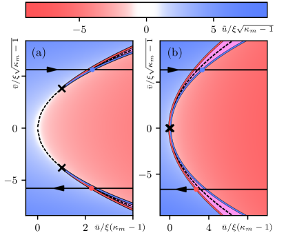
Figure 14: Bistable domain $\mathcal{B}_{\bar{\bf R}}$ in asymptotic space $\bar{\bf R}$ before (a) and after (b) merging, for $1-\kappa_{s}=\pm 0.01$ and parameters as in Fig. 13. (a) Before merging, the bistable domain $\mathcal{B}_{\bar{\bf R}}$ consists of two parts, corresponding to the two unstable regions $\mathcal{U}_{\tilde{\bf R}}$ in Fig. 13(a). These terminate in the cusps at $\bar{\bf R}_{s,c,\pm}^{<}$ that approach one another along the dashed parabola (139) to merge at $\kappa_{s}=1$. Red/blue colors indicate different vortex configurations as quantified through the order parameter $\tilde{u}-\tilde{u}_{m}(\bar{v})$, while magenta is associated to the bistable region $\mathcal{B}_{\bar{\bf R}}$. Colored dots mark the asymptotic positions associated to the pairs of jump positions in Fig. 13(a). (b) After merging, the bistable domain is continuously connected; the cusps/critical points have vanished and the dashed parabola turns into the branch cutting line. The black crosses now mark the positions of strongest pinching of $\mathcal{B}_{\bar{\bf R}}$, the colored dots mark the asymptotic positions associated to the pairs of tip positions in Fig. 13(b).

The set of asymptotic positions corresponding to $\mathcal{U}_{\tilde{\bf R}}$ before and after merging, i.e., the bistable domain $\mathcal{B}_{\bar{\bf R}}$, can be found by systematically repeating the steps in Sec. III.3. Applying the force balance equation $\nabla_{\mathbf{R}}e_{\mathrm{pin}}(\mathbf{R};\bar{\bf R})\Big{|}_{\tilde{\bf R}}=0$ to the energy expansion (V.1), we find the counterpart of Eqs. (69),

$$\bar{C}\bar{u} =\bar{C}(1-\kappa_{s})\tilde{u}+\frac{a_{s}}{2}\tilde{v}^{2}+\frac{\gamma_{s}}{6}\tilde{u}^{3}+\frac{\beta_{s}}{2}\tilde{u}^{2}\tilde{v}+\frac{\alpha_{s}}{2}\tilde{u}\tilde{v}^{2},$$

$$\bar{C}\bar{v} =(\bar{C}+\lambda_{s,+})\tilde{v}+a_{s}\,\tilde{u}\tilde{v}+\frac{\beta_{s}}{6}\tilde{u}^{3}+\frac{\alpha_{s}}{2}\tilde{u}^{2}\tilde{v},$$ (137)

relating tip and asymptotic positions close to merging. As for the unstable domain, the topology of $\mathcal{B}_{\bar{\bf R}}$ depends on the sign of $1-\kappa_{s}$. The bistable domain $\mathcal{B}_{\bar{\bf R}}$ before merging is shown in Fig. 14(a) for $1-\kappa_{s}=0.01$. It consists of two parts, corresponding to the two pieces of $\mathcal{U}_{\tilde{\bf R}}$ for $1-\kappa_{s}>0$, that terminate at the cusps $\bar{\bf R}_{s,c,\pm}^{<}$. The latter are related to the vertices $\tilde{\bf R}_{s,c,\pm}^{<}$ of the jumping hyperbola through the force balance equation (137),

$$\delta\bar{\bf R}_{s,c,\pm}^{<}\approx\left[\left(a_{s}/2\,\bar{C}\right)\,\tilde{v}^{2}_{s,c},\,\pm\left(1+\lambda_{s,+}/\bar{C}\right)\tilde{v}_{s,c}\right].$$ (138)

For finite values of $(1-\kappa_{s})$, the cusps are separated by a distance $2|\delta{\bar{\bf R}}_{s,c,\pm}^{<}|\approx 2\left(1+\lambda_{s,+}/\bar{C}\right)\tilde{v}_{s,c}\propto\sqrt{1-\kappa_{s}}$. They approach one another along the parabola

$$\bar{u}_{s,0}\approx\frac{a}{2\bar{C}}\frac{1}{(1+\lambda_{+}/\bar{C})^{2}}\bar{v}_{s,0}^{2},$$ (139)

see the black dashed line in Fig. 14, with higher-order corrections appearing at finite skew $\beta\neq 0$. After merging, this line lies within $\mathcal{B}_{\bar{\bf R}}$ and defines the branch crossing line, cf. Eq. (77).

After merging, when $\kappa_{s}-1>0$, the cusps have vanished and the edges have rearranged to define a connected bistable region, see Fig. 14(b). The extremal points of the two edges are found by evaluating the force balance equation (137) at the vertices $\tilde{\bf R}_{s,e,\pm}^{>}$, Eq. (129), to lowest order,

$$\delta\bar{\bf R}_{s,e,\pm}^{>}\approx\frac{\beta_{s}}{\delta_{s}}\left[\frac{a_{s}}{2\,\bar{C}}\frac{\beta_{s}}{\delta_{s}}\,\tilde{u}_{s,e}^{2},\,\mp\left(1+\frac{\lambda_{s,+}}{\bar{C}}\right)\,\tilde{u}_{s,e}\right].$$ (140)

For finite values of $(\kappa_{s}-1)$, these points are separated by a distance $2|\delta\bar{\bf R}_{s,e,\pm}^{>}|\approx 2\left(1+\lambda_{s,+}/\bar{C}\right)(\beta_{s}/\delta_{s})\tilde{u}_{s,e}\propto\sqrt{\kappa_{s}-1}$. Note that the extremal points $\bar{\bf R}_{s,e,\pm}^{>}$ are no longer associated to cusps or critical points as these have disappeared in the merging process. When the skew parameter vanishes as in Fig. 14, $\beta_{s}=0$, higher-order terms in $(\kappa_{s}-1)$ in the force-balance equation (137) become relevant in determining the positions $\bar{\bf R}_{s,e,\pm}^{>}$, separating them along the unstable $u$-direction. In this case, we obtain a different scaling for their distance, i.e., $|\delta\bar{\bf R}_{s,e,\pm}^{>}|\propto\left(1-\kappa_{s}\right)^{3/2}$.

V.4 Topological aspect of mergers

In order to discuss the topological aspect of a merger, it is convenient to consider some specific examples. In Sec. IV, we have analyzed the case of a uniaxial defect with a quadrupolar anisotropy $\delta e_{p}\propto\epsilon\sin^{2}\tilde{\phi}$ in the pinning potential, see (105), that produced a degenerate onset at symmetric points $[\pm\tilde{x}_{m},0]$. Here, we choose again a weakly anisotropic defect centered in the origin but with a dipolar deformation $\delta e_{p}\propto\epsilon\cos\tilde{\phi}$ that results in an angle-dependent Labusch parameter

$$\kappa_{m}(\tilde{\phi})=\kappa_{m}-\epsilon\cos\tilde{\phi},$$ (141)

see Eq. (107). The strong pinning onset of such a defect then appears in an isolated point on the negative $x$-axis, with the unstable ellipse $\mathcal{U}_{\tilde{\bf R}}$ deforming with increasing $\kappa_{m}$ into a horseshoe that is open on the positive $x$-axis—the closing of the horseshoe to produce a ring, see Fig. 15, then corresponds to the local merger shown in Fig. 13. With this example in mind, we can repeat the discussion in Sec. III.5: The unstable eigenvector $\mathbf{v}_{-}(\mathbf{R}_{\mathrm{jp}})$ points radially outwards from the origin over the entire horseshoe, including the merging region at positive $x$. On the other hand, the tangent to the boundary $\partial\mathcal{U}_{\tilde{\bf R}}$ rotates forward and back along the horseshoe as shown in Fig. 15 (we attribute a direction to $\partial\mathcal{U}_{\tilde{\bf R}}$ with the convention of following the boundary with the unstable region on the left); in fact, over most of the boundary, the tangent is simply orthogonal to $\mathbf{v}_{-}$, with both vectors rotating together when going along $\partial\mathcal{U}_{\tilde{\bf R}}$. At the ends of the horseshoe, however, the tangent locally aligns parallel (anti-parallel) to $\mathbf{v}_{-}$ and the two vectors rotate (anti-clockwise) with respect to one another, with the total winding equal to $2\pi$. After the merger, this winding has disappeared, with the resulting ring exhibiting no winding in the tangent fields on the inner/outer boundary; as a result, the contact points between the jump and landing lines have disappeared.

Furthermore, the merger changes the topology of $\mathcal{U}_{\tilde{\bf R}}$ from the simply-connected horseshoe to the non-simply connected ring, while the number of components in $\mathcal{U}_{\tilde{\bf R}}$ has not changed. Note that the change in the relative winding is not due to crossing the singularity of the vector field $\mathbf{v}_{-}$ as alluded to in Sec. III.5—rather, it is the merger of the horseshoe tips that rearranges the boundaries of $\mathcal{U}_{\tilde{\bf R}}$ and make them encircle the singularity.

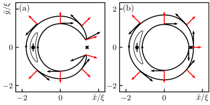
Figure 15: Left: Unstable region $\mathcal{U}_{\tilde{\bf R}}$ for a defect with dipolar asymmetry. Upon the onset of strong pinning, an unstable ellipse appears to the left of the defect center (black solid dot). With increasing pinning strength (decreasing $\bar{C}$) the ellipse grows and deforms into a horseshoe geometry. The unstable eigenvector field $\mathbf{v}_{-}$ (red arrows) points radially outward away from the defect center. The tangent field to the boundary $\partial\mathcal{U}_{\tilde{\bf R}}$ (black arrows) follows the unstable direction at an angle of $\pi/2$ over most of $\partial\mathcal{U}_{\tilde{\bf R}}$, with the exception of the two turning points where the tangent rotates by $\pi$ with respect to $\mathbf{v}_{-}$, producing a relative winding of $2\pi$. Right: After the merger of the turning points the unstable region $\mathcal{U}_{\tilde{\bf R}}$ changes topology and assumes the shape of a ring. The windings of the tangent field with respect to the eigenvector-field $\mathbf{v}_{-}$ vanish separately for both boundaries of $\mathcal{U}_{\tilde{\bf R}}$.

In the above example, we have discussed a merger that changes the connectedness of $\mathcal{U}_{\tilde{\bf R}}$. On the other hand, as we are going to show, a merger might leave the connectedness of $\mathcal{U}_{\tilde{\bf R}}$ unchanged, while modifying the number of components, i.e., the number of disconnected parts, in $\mathcal{U}_{\tilde{\bf R}}$. Let us again consider a specific example in the form of an anisotropic defect with a warped well shape, producing several (in general subsequent) onsets and mergers; in Fig. 16, we consider a situation with three onset points and subsequent individual mergers. After the onset, the three ellipses define an unstable region $\mathcal{U}_{\tilde{\bf R}}$ with three disconnected parts that are simply-connected each. This configuration is characterized by its number of components measuring $C=3$. As two of the three ellipses merge, the number of components of $\mathcal{U}_{\tilde{\bf R}}$ reduces to $C=2$, the next merger generates a horseshoe that is still simply-connected with $C=1$. The final merger produces a ring; while the number of components remains unchanged, $C=1$, the unstable area assumes a non-simply connected shape with a ‘hole’; we associate the index $H=1$ with the appearance of this hole within $\mathcal{U}_{\tilde{\bf R}}$. In physics terms, the last merger producing a hole in $\mathcal{U}_{\tilde{\bf R}}$ is associated with the appearance of a pinned state; the unstable ring separates stable tip positions that are associated with pinned and free vortex configurations residing at small and large radii, respectively.

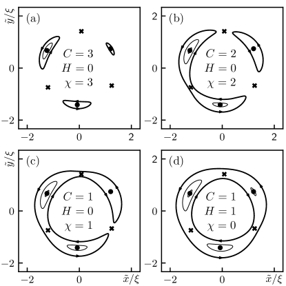
Figure 16: The unstable domain $\mathcal{U}_{\tilde{\bf R}}$ starting out with $C=3$ components in (a) changes topology in three steps: after the first (b) and second (c) mergers the number of components $C$ has changed from three in (a) to two in (b) to one in (c), leading to a horseshoe shape of $\mathcal{U}_{\tilde{\bf R}}$. The third merger closes the horseshoe to produce the ring geometry in (d) characterized by the coefficients $C=1$ and $H=1$ ($H$ denotes the number of ‘holes’ in $\mathcal{U}_{\tilde{\bf R}}$); the Euler characteristic $\chi=C-H$ changes by unity in every merger.

Defining the (topological) characteristic $\chi\equiv C-H$, we see that $\chi$ changes by unity at every onset and merger, either through an increase (for an onset) or decrease (for a merger) in the number of components $C\to C\pm 1$, or through the appearance of a hole (in a merger) $H\to H+1$. Indeed, the quantity $\chi$ is known as the Euler characteristic of a manifold and describes its global topological properties; it generalizes the well known Euler characteristic of a polyhedron to surfaces and manifoldsNakahara (2003), see Sec. VI below. Finally, Morse theory Nash and Sen (2011) connects the Euler characteristic with the local differential properties (minima, maxima, saddles) of that manifold, hence establishing a connection between local onsets and mergers (at minima and saddles of $D(\tilde{\bf R})$) and the global properties of $\mathcal{U}_{\tilde{\bf R}}$ such as the appearance of new pinned states. In Sec. VI below, we consider the general case of a random pinning landscape in two dimensions and discuss the connection between local differential and global topological properties of $\mathcal{U}_{\tilde{\bf R}}$ in the light of Morse theory—the topology of bistable domains $\mathcal{B}_{\bar{\bf R}}$ then follows trivially.

VI $\mathcal{U}_{\tilde{\bf R}}$ of a two-dimensional pinscape

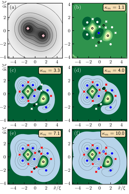
Figure 18: (a) Grayscale image of the pinning potential landscape $e_{p}(\tilde{\bf R})$, with the two diamonds marking the positions of the defects. (b)–(f) Shifted curvature function $\Lambda_{\bar{C}}(\tilde{\bf R})$ (in topographic coloring, see caption of Fig. 17) versus tip position $\tilde{\bf R}$ for increasing values of $\kappa_{m}$ as we proceed from (b) to (f). The pinscape in (a) produces a curvature landscape with $6$ minima (solid dots), $4$ maxima (open dots), and $9$ saddles (crosses). Upon increasing $\kappa_{m}$, several unstable regions $\mathcal{U}_{\tilde{\bf R}}$ appear (solid dots turn blue) and merge (crosses turn red) to change the topology of $\mathcal{U}_{\tilde{\bf R}}$. The Euler characteristic $\chi(\mathcal{U}_{\tilde{\bf R}})=m-s+M=1=C$ in (b), remains $\chi(\mathcal{U}_{\tilde{\bf R}})=1$ in (c), but with $C=2$ and $H=1$, changes to $\chi(\mathcal{U}_{\tilde{\bf R}})=-1$ in (d), and $\chi(\mathcal{U}_{\tilde{\bf R}})=-3$ with one component $C=1$ and four holes $H=4$ in (e). In going from (e) to (f) two of the maxima (black open dots turn blue) drop below zero, producing a characteristic $\chi(\mathcal{U}_{\tilde{\bf R}})=6-9+2=-1$; indeed, $\mathcal{U}_{\tilde{\bf R}}$ in (f) has one component $C=1$ and two holes $H=2$, reproducing $\chi(\mathcal{U}_{\tilde{\bf R}})=C-H=-1$.

We consider a two-dimensional pinning landscape $e_{p}(\mathbf{R})$, e.g., as produced by a superposition of several (anisotropic Lorentzian) defects residing in the $z=0$ plane. In the figures 17 and 18, we analyse two specific cases with $n=3$ and $n=2$ defects as given in Eq. (94) with $\epsilon=0.1$ and positions listed in Tables 1 and 2; these produce unstable landscapes $\mathcal{U}_{\tilde{\bf R}}$ of considerable complexity already, see Figs. 17(a) and 18(a). Our defects are compact with $e_{p}(\mathbf{R})\to 0$ vanishing at $R\to\infty$; as a result, $e_{\mathrm{pin}}$ becomes flat at infinity. Note that a dense assembly of uniformly distributed individual defects produces a random Gaussian pinning landscape, as has been shown in Ref. Willa et al., 2022.

Here, we are interested in the evolution of the unstable and bistable domains $\mathcal{U}_{\tilde{\bf R}}$ and $\mathcal{B}_{\bar{\bf R}}$ associated with the 2D pinning landscape $e_{\mathrm{pin}}$; we focus on the unstable domain $\mathcal{U}_{\tilde{\bf R}}$, with the properties of the bistable domain $\mathcal{B}_{\bar{\bf R}}$ following straightforwardly from the solution of the force balance equation (2). Unlike the analysis above that is centered on special points of $\mathcal{U}_{\tilde{\bf R}}$, ellipses near onset and hyperbolas near mergers, here, we are interested in the global properties of the unstable region produced by a generic (though still two-dimensional) pinscape.

As discussed in Sec. III above, the unstable region $\mathcal{U}_{\tilde{\bf R}}$ associated with strong pinning is determined by the condition $D(\tilde{\bf R})=0$ of vanishing Hessian determinant, more precisely, by the competition between the lowest eigenvalue $\lambda_{-}(\tilde{\bf R})$ of the Hessian matrix $\mathrm{H}_{ij}$ of the pinning potential $e_{p}(\mathbf{R})$ and the effective elasticity $\bar{C}$, see Eq. (37). In order to avoid the interference with the second eigenvalue $\lambda_{+}(\tilde{\bf R})$ of the Hessian matrix, we consider the shifted (by $\bar{C}$) curvature function

$$\Lambda_{\bar{C}}(\tilde{\bf R})\equiv\bar{C}+\lambda_{-}(\tilde{\bf R}),$$ (142)

i.e., the relevant factor of the determinant $D(\tilde{\bf R})=[\bar{C}+\lambda_{-}(\tilde{\bf R})][\bar{C}+\lambda_{-}(\tilde{\bf R})]$. The condition

$$\Lambda_{\bar{C}}(\tilde{\bf R})=0$$ (143)

then determines the boundaries of $\mathcal{U}_{\tilde{\bf R}}$.

Table 1: Positions and relative weights of 3 uniaxially anisotropic Lorentzian defects in Fig. 17 as given by Eq. (94).

	$~{}x/\xi$	$y/\xi$	weight
defect #1	$1.14$	$1.07$	0.65
defect #2	$-0.98$	$-0.19$	1
defect #3	$0.20$	$-0.67$	1

Table 2: Positions and relative weights of 2 uniaxially anisotropic Lorentzian defects in Fig. 18 as given by Eq. (94).

	$~{}x/\xi$	$y/\xi$	weight
defect #1	$-1.32$	$0.33$	1
defect #2	$1.48$	$-0.76$	1

The above problem can be mapped to the problem of cutting a surface, where $\Lambda_{\bar{C}}(\tilde{\bf R})$ is interpreted as a height-function over $\mathbb{R}^{2}$ that is cut at zero level; the elasticity $\bar{C}$ then plays the role of a shift parameter that moves the function $\lambda_{-}(\tilde{\bf R})$ downwards in height with decreasing $\bar{C}$ (that corresponds to increasing the relative pinning strength of the pinscape in physical terms). As $\bar{C}$ is decreased to compensate the absolute minimum of $\lambda_{-}(\tilde{\bf R})<0$, $\bar{C}+\lambda_{-}(\tilde{\bf R})=0$, strong pinning sets in locally at $\tilde{\bf R}_{m}$ for the first time in the form of an unstable ellipse $\mathcal{U}_{\tilde{\bf R}}$, see Fig. 17(b) for our specific example with three defects; the Labusch parameter $\kappa(\tilde{\bf R})$ evaluated at the point $\tilde{\bf R}_{m}$ defines $\kappa_{m}$, the parameter tuned in Fig. 17. Decreasing $\bar{C}$ further, this ellipse grows and deforms, while other local minima of $\lambda_{-}(\tilde{\bf R})$ produce new disconnected parts of $\mathcal{U}_{\tilde{\bf R}}$, a situation illustrated in Fig. 17(c) where four ‘ellipses’ have appeared around (local) minima (blue filled dots). A further increase in pinning strength (decrease in $\bar{C}$) continuous to deform these ‘ellipses’ and adds three new ones. As the first saddle drops below the zero level (red cross), two components merge and the number of components decreases; in Fig. 17(d), we have three below-zero saddles and only four components remain, $C=4$. In Fig. 17(e) four further mergers have reduced $C$ to 1 as the corresponding saddles drop below zero level. This produces a single non-simply connected component, i.e., $C=1$ and a hole, increasing the number of holes $H$ from zero to one. The last merger leading to (f) finally leaves $C=1$ but cuts the stable region inside the ring into two, increasing the number of holes to $H=2$.

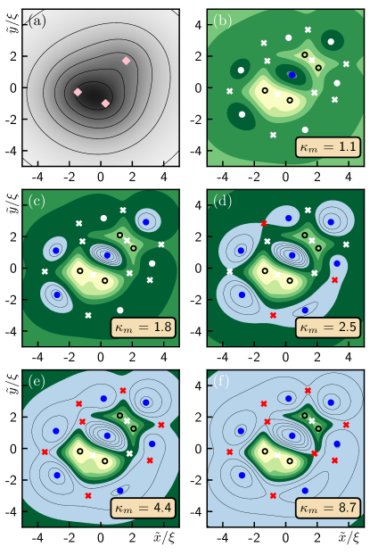
Figure 17: (a) Grayscale image of the pinning potential landscape $e_{p}(\tilde{\bf R})$, with the three diamonds marking the positions of the defects. (b)–(f) Shifted curvature function $\Lambda_{\bar{C}}(\tilde{\bf R})$ versus tip position $\tilde{\bf R}$ for increasing values of $\kappa_{m}$ (decreasing $\bar{C}$) as we proceed from (b) to (f). We make use of the topographic interpretation with positive values of $\Lambda_{\bar{C}}$ marked as landmass (greenish colors, with low/high elevation in dark/light green) and negative values of $\Lambda_{\bar{C}}$ constituting $\mathcal{U}_{\tilde{\bf R}}$ in flat light blue (height levels are shown by thin black lines). The pinscape in (a) produces a curvature landscape with $7$ minima (solid dots), $4$ maxima (open dots), and $10$ saddles (crosses). Several unstable regions $\mathcal{U}_{\tilde{\bf R}}$ appear (solid dots turn blue) and merge (crosses turn red) to change the topology of $\mathcal{U}_{\tilde{\bf R}}$. The Euler characteristic $\chi(\mathcal{U}_{\tilde{\bf R}})=m-s+M=1-0+0=1$ in (b) changes to $\chi(\mathcal{U}_{\tilde{\bf R}})=4$ in (c) and (d), drops to $\chi(\mathcal{U}_{\tilde{\bf R}})=0$ in (e) and $\chi(\mathcal{U}_{\tilde{\bf R}})=-1$ in (f); indeed, $\mathcal{U}_{\tilde{\bf R}}$ in (f) has one component $C=1$ and two holes $H=2$, reproducing $\chi(\mathcal{U}_{\tilde{\bf R}})=C-H=-1$.

This sequence of onsets and mergers is conveniently described in the topographic language introduced in section IV that interprets stable tip regions as land mass (green with bright regions indicating higher mountains in Fig. 17) and unstable regions as lakes (flat blue with (below-water) height levels indicated by thin black lines), with the height $\Lambda_{\bar{C}}=0$ defining the water level. The sequence (b) to (f) then shows the flooding of the landscape as pinning increases ($\bar{C}$ decreasing), with white dot minima turning blue at strong pinning onsets and white cross saddles turning red at mergings; maxima in the landscape are shown as black open circles. Note that we distinguish critical points (minima, saddles) residing below (blue and red) and above (white) water level. Similarly, a (local) maximum above sea level (black open dot) turns into a blue open dot as it drops belop sea level; such an event is missing in Fig. 17 but can be produced with other configurations of defects, see Fig. 18 where the curvature landscape for two defects is shown.

The above discussion relates the local differential properties of the function $\Lambda_{\bar{C}}(\tilde{\bf R})<0$, minima and saddles, to the global topological properties of $\mathcal{U}_{\tilde{\bf R}}$, its number of components $C(\mathcal{U}_{\tilde{\bf R}})$ and holes $H(\mathcal{U}_{\tilde{\bf R}})$. This connection between local and global properties is conveniently discussed within Morse theory Nash and Sen (2011). Before presenting a general mathematical formulation, let us discuss a simple heuristic argument producing the result relevant in the present context; in doing so, we make use of the above topographic language.

Starting with the minima of the function $\Lambda_{\bar{C}}(\tilde{\bf R})$, a new disconnected component appears in $\mathcal{U}_{\tilde{\bf R}}$ whenever the minimum drops below sea level as $\bar{C}$ is decreased, that produces an increase $C\to C+1$. With the further decrease of $\bar{C}$, these disconnected regions expand and merge pairwise whenever a saddle point of $\Lambda_{\bar{C}}(\tilde{\bf R})$ goes below sea level, thereby inducing a change in the topology of $\mathcal{U}_{\tilde{\bf R}}$ by either reducing the number of components $C\to C-1$ (keeping $H$ constant) or leaving it unchanged (changing $H\to H+1$), see, e.g., the example with the horseshoe closing up on itself in Sec. V.4. The below sea-level minima and saddles of $\Lambda_{\bar{C}}(\tilde{\bf R})$ can naturally be identified with the vertices and edges of a graph; the edges in the graph then define the boundaries of the graph’s faces (the same way as the vertices are the boundaries of the edges). For a connected graph, Euler’s formula then tells us that the number $V$ of vertices, $E$ of edges, and $F$ of faces are constrained via $V-E+F=1$ (not counting the outer face extending to infinity) and a graph with $C$ components satisfies the relation $C=V-E+F$ as follows from simple addition.

We have already identified minima and saddles of $\Lambda_{\bar{C}}(\tilde{\bf R})<0$ with vertices and edges of a graph; denoting the number of below sea-level minima and saddles by $m$ and $s$, we have $V=m$ and $E=s$. It remains to express the number $F$ of faces in terms of critical points of the surface $\Lambda_{\bar{C}}(\tilde{\bf R})<0$. Indeed, the faces of our graph are associated with maxima of the function $\Lambda_{\bar{C}}(\tilde{\bf R})$: following the boundaries of a face, we cross the corresponding saddles with the function $\Lambda_{\bar{C}}(\tilde{\bf R})$ curving upwards away from the edges, implying that the faces of our graph include maxima of $\Lambda_{\bar{C}}(\tilde{\bf R})$. These maxima manifest in two possible ways: either the face contains a single below sea-level maximum or a single above sea-level landscape. The above sea-level landscape comprises at least one maximum but possibly also includes other extremal points that we cannot analyse with our knowledge of the below sea-level function $\Lambda_{\bar{C}}(\tilde{\bf R})<0$ only; we therefore call the above sea-level landscape a (single) hole. The appearance of a single maximum or hole is owed to the fact that faces are not split by a below sea-level saddle as these have already been accounted for in setting up the graph.

Let us denote the number of (below sea-level) maxima by $M$ and the number of holes by $H$, then $F=H+M$. Combining this last expression with Euler’s formula and regrouping topological coefficients $C(\mathcal{U}_{\tilde{\bf R}})$ and $H(\mathcal{U}_{\tilde{\bf R}})$ on one side and extremal points $m[\Lambda_{\bar{C}}(\tilde{\bf R})]$, $s[\Lambda_{\bar{C}}(\tilde{\bf R})]$, and $M[\Lambda_{\bar{C}}(\tilde{\bf R})]$ on the other, we arrive at the Euler characteristic $\chi\equiv C-H$ and its representation through local differential properties,

$$\chi(\mathcal{U}_{\tilde{\bf R}})\equiv[C-H]_{\mathcal{U}_{\tilde{\bf R}}}=[m-s+M]_{\Lambda_{\bar{C}}(\tilde{\bf R})<0}.$$ (144)

The result (144) follows rigorously from the Euler-Poincaré theoremNakahara (2003); Nash and Sen (2011) in combination with Morse’s theorem Nash and Sen (2011), with the former expressing the Euler characteristic $\chi(\mathcal{U}_{\tilde{\bf R}})$ through the so-called Betti numbers $b_{i}(\mathcal{U}_{\tilde{\bf R}})$,

$$\chi(\mathcal{U}_{\tilde{\bf R}})\equiv\sum_{i=0}^{2}(-1)^{i}b_{i}(\mathcal{U}_{\tilde{\bf R}}),$$ (145)

where the $i$-th Betti number $b_{i}(\mathcal{U}_{\tilde{\bf R}})=\mathrm{Dim}[H_{i}(\mathcal{U}_{\tilde{\bf R}})]$ is given by the dimension or rank of the $i$-th (singular) homology group $H_{i}(\mathcal{U}_{\tilde{\bf R}})$. In colloquial terms, the Betti numbers $b_{i}$ count the number of ‘holes’ in the manifold with different dimensions $i$: the zeroth Betti number gives the number of components $b_{0}=C$ of $\mathcal{U}_{\tilde{\bf R}}$, the first Betti number $b_{1}=H$ counts the holes, and the second Betti number refers to cavities, here $b_{2}=0$ for our open manifold. Hence, we find that the Euler characteristic is given by the number of components and holes in $\mathcal{U}_{\tilde{\bf R}}$,

$$\chi(\mathcal{U}_{\tilde{\bf R}})=C(\mathcal{U}_{\tilde{\bf R}})-H(\mathcal{U}_{\tilde{\bf R}}),$$ (146)

in agreement with the discussion in Sec. V.4 and (144).

Morse theoryNash and Sen (2011) then provides a connection between the topological properties of the manifold $\mathcal{U}_{\tilde{\bf R}}$ and the local differential properties of the surface $\Lambda_{\bar{C}}(\tilde{\bf R})<0$ defining it: with $C_{i}$ the number of critical points with index $i$ of the surface $\Lambda_{\bar{C}}(\tilde{\bf R})<0$ (the index $i$ counts the number of negative eigenvalues of the Hessian matrix evaluated at the critical point), the Euler characteristic $\chi(\mathcal{U}_{\tilde{\bf R}})$ relates the manifold’s topology to the number and properties of critical points,

$$\chi(\mathcal{U}_{\tilde{\bf R}})=\sum_{i=0}^{2}(-1)^{i}C_{i}(\Lambda_{\bar{C}}<0).$$ (147)

For our 2D manifold the coefficients $C_{i}$ count the minima $C_{0}=m$, the number of saddles $C_{1}=s$, and $C_{2}=M$ refers to the number of maxima, hence,

$$\chi(\mathcal{U}_{\tilde{\bf R}})=[m-s+M]_{\Lambda_{\bar{C}}<0}$$ (148)

and the combination with (146) produces the result (144) anticipated above.

Summarizing, knowing the number of critical points $m$, $M$, and $s$ of the seascape, i.e., its local differential properties, we can determine the global topological aspects of the pinning landscape via the evaluation of the Euler characteristic $\chi(\mathcal{U}_{\tilde{\bf R}})$ with the help of Eq. (148). The latter then informs us about the number $C$ of unstable domains in $\mathcal{U}_{\tilde{\bf R}}$ where locally pinned states appear and the number of holes $H$ in $\mathcal{U}_{\tilde{\bf R}}$ where globally distinct pinned states show up. Furthermore, the outer boundaries of the lakes, of which we have $C$ components, are to be associated with instabilities of the free vortex state, while inner boundaries (or boundaries of holes, which count $H$ elements) tell about instabilities of pinned states, hence the Betti numbers $C$ and $H$ count different types of instabilities. It would then have been nice to determine the separate topological coefficients $C$ and $H$ individually—unfortunately, $\chi(\mathcal{U}_{\tilde{\bf R}})$ as derived from local differential properties provides us only with the difference $C-H$ between locally and globally pinned areas and not their individual values. Nevertheless, using Morse theory, we could connect our discussion of local differential properties of the pinning landscape in Secs. III.1 and V.1 with the global pinning properties of the pinning energy landscape as expressed through the topology of the unstable domain $\mathcal{U}_{\tilde{\bf R}}$.

Regarding our previous examples, the isotropic and uniaxial defects, we remark that for the latter the two simultaneous mergers on the $y$-axis produce a reduction in $C=2\to 1$ and an increase of $H=0\to 1$ and hence a jump from $\chi=2$ to $\chi=0$ in one step, as expected for two simultaneous mergers. The symmetry of the isotropic defect produces a (degenerate) critical line at $\tilde{R}_{m}$ rather than a critical point; adding a small perturbation $\propto x^{3}$ breaks this symmetry and produces the horseshoe geometry discussed in Sec. V.4 above that is amenable to the standard analysis.

A last remark is in place about the topological properties in dual space, i.e., of bistable regions $\mathcal{B}_{\bar{\bf R}}$. Here, the mergers produce another interesting phenomenon as viewed from the perspective of its thermodynamic analogue. Indeed, the merger of deformed ellipses in tip-space corresponds to the merger of cusps in asymptotic space, what translates to the vanishing of critical points and a smooth continuation of the first-order critical and spinodal lines in the thermodynamic analogue, see also Sec. V.3. We are not aware of a physical example in thermodynamics that produces such a merger and disappearance of critical points.

VII Summary and outlook

Strong pinning theory is a quantitative theory describing vortex pinning in the dilute defect limit where this complex many-body system can be reduced to an effective single-pin–single-vortex problem. The accuracy offered by this theory then allows for a realistic description of the shape of the pinning potential $e_{p}(\mathbf{R})$ associated with the defects. While previous work focused on the simplest case of isotropic defects, here, we have generalized the strong pinning theory to the description of arbitrary anisotropic pinning potentials. Surprisingly, going from an isotropic to an anisotropic defect has quite astonishing consequences for the physics of strong pinning—this reminds about other physical examples where the removal of symmetries or degeneracies produces new effects.

While the strong pinning problem is quite a complex one requiring the use of numerical tools in general, we have identified several generic features that provide the essential physics of the problem and that are amenable to an analytic treatment. Specifically, these are the points of strong pinning onset and the merger points, around which the local expansions of the pinning potential $e_{\mathrm{pin}}(\tilde{\bf R};\bar{\bf R})$ in the tip coordinate $\tilde{\bf R}$ allow us to find all the characteristics of strong pinning. In particular, we identify the instability region $\mathcal{U}_{\tilde{\bf R}}$ in the vortex tip space (with coordinates $\tilde{\bf R}$) and the bistable region $\mathcal{B}_{\bar{\bf R}}$ in the space of asymptotic vortex positions $\bar{\bf R}$ as the main geometric objects that determine the critical pinning force density $F_{\mathrm{pin}}$, from which the critical current density $j_{c}$, the technologically most relevant quantity of the superconductor, follows straightforwardly. While the relevance of the bistable region $\mathcal{B}_{\bar{\bf R}}$ was recognized in the past Labusch (1969); Larkin and Ovchinnikov (1979); Blatter et al. (2004), the important role played by the unstable region $\mathcal{U}_{\tilde{\bf R}}$ went unnoticed so far.

When going from an isotropic defect to an anisotropic one, the strong pinning onset changes dramatically: while the unstable region $\mathcal{U}_{\tilde{\bf R}}$ grows out of a circle of radius $\sim\xi$ and assumes the shape of a ring at $\kappa>1$ for the isotropic situation, for an anisotropic defect the onset appears in a point $\tilde{\bf R}_{m}$ and grows in the shape of an ellipse with increasing $\kappa_{m}>1$; the location where this onset appears is given by the Hessian of $e_{\mathrm{pin}}$, specifically, the point $\tilde{\bf R}_{m}$ where its determinant touches zero first, $\det\{\mathrm{Hess}[e_{\mathrm{pin}}(\tilde{\bf R};\bar{\bf R})|_{\bar{\bf R}}]\}_{\tilde{\bf R}_{m}}=0$. The boundary of this ellipse defines the jump positions $\mathcal{J}_{\mathrm{\tilde{\bf R}}}$ associated with the strong pinning instabilities; when combined with the landing ellipse $\mathcal{L}_{\mathrm{\tilde{\bf R}}}$, these two ellipses determine the jump distance $\delta\tilde{u}$ of the vortex tip, from which follows the jump in the pinning energy $\Delta e_{\mathrm{pin}}\propto\delta\tilde{u}^{4}$, which in turn determines $F_{\mathrm{pin}}$ and $j_{c}$.

The bistable region $\mathcal{B}_{\bar{\bf R}}$ in asymptotic vortex space comes into play when calculating the average critical force density $F_{\mathrm{pin}}$ opposing the vortex motion: while the vortex tip undergoes a complex trajectory including jumps, the vortex motion in asymptotic space $\bar{\bf R}$ is described by a straight line. As this trivial trajectory in $\bar{\bf R}$-space traverses the bistable region $\mathcal{B}_{\bar{\bf R}}$, the vortex tip jumps upon exiting $\mathcal{B}_{\bar{\bf R}}$, that produces the jump $\Delta e_{\mathrm{pin}}$ and hence $F_{\mathrm{pin}}$. Again, the shape of $\mathcal{B}_{\bar{\bf R}}$ changes when going from the isotropic to the anisotropic defect, assuming a ring of finite width around a circle of radius $\sim\xi$ in the former case, while growing in the form of a crescent out of a point for the anisotropic defect.

The new geometries associated with $\mathcal{U}_{\tilde{\bf R}}$ and $\mathcal{B}_{\bar{\bf R}}$ then produce a qualitative change in the scaling behavior of the pinning force density $F_{\mathrm{pin}}\propto(\kappa_{m}-1)^{\mu}$ near onset, with the exponent $\mu$ changing from $\mu=2$ to $\mu=5/2$ when going from the isotropic to the anisotropic defect. This change is due to the change in the scaling of the geometric size of $\mathcal{B}_{\bar{\bf R}}$, with the replacement of the fixed radius $\sim\xi$ of the ring by the growing size of the crescent $\sim\xi(\kappa_{m}-1)^{1/2}$ [the exponent $\mu$ assumes a value $\mu=3$ for trajectories cutting the crescent along its short dimension of size $\xi(\kappa_{m}-1)$]. Furthermore, for directed defects, the pinning force density $F_{\mathrm{pin}}(\theta)$ depends on the impact angle $\theta$ relative to the unstable direction $u$ and is aligned with $u$, except for a small angular regime close to $\theta=\pi/2$. This results in a pronounced anisotropy in the critical current density $j_{c}$ in the vicinity of the strong pinning onset.

A fundamental difference between the strong pinning onsets in the isotropic and in the anisotropic case are the geometries of the unstable $\mathcal{U}_{\tilde{\bf R}}$ and bistable $\mathcal{B}_{\bar{\bf R}}$ regions: these are non-simply connected for the isotropic case (rings) but simply connected for the anisotropic defect (ellipse and crescent). The resolution of this fundamental difference is provided by the second type of special points, the mergers. Indeed, for a general anisotropic defect, the strong pinning onset appears in a multitude of points, with unstable and bistable regions growing with $\kappa_{m}>1$ and finally merging into larger areas. Two examples illustrate this behavior particularly well, the uniaxial defects with a quadrupolar and a dipolar deformation, see Secs. IV and V.4. In the first case, symmetric onset points on the $x$ axis produce two ellipses/crescents that grow, approach one another, and finally merge in a ring-shaped geometry that is non-simply connected. In the case of a dipolar deformation, we have seen $\mathcal{U}_{\tilde{\bf R}}$ grow out of a single point with its ellipse expanding and deforming around a circle, assuming a horseshoe geometry, that finally undergoes a merging of the two tips to produce again a ring; similar happens when multiple $\mathcal{U}_{\tilde{\bf R}}$ domains grow and merge as in Figs. 16 (a warped defect) and 18(c) (a 2D pinning landscape where four unstable domains have merged to enclose an ‘island’).

These merger points are once more amenable to an analytic study using a proper expansion of $e_{\mathrm{pin}}(\tilde{\bf R};\bar{\bf R})$ in $\tilde{\bf R}$ around the merger point $\tilde{\bf R}_{s}$, the latter again defined by the local differential properties of the determinant $\det\{\mathrm{Hess}[e_{\mathrm{pin}}(\tilde{\bf R};\bar{\bf R})|_{\bar{\bf R}}]\}$, this time not a minimum but a saddle. Rather than elliptic as at onset, at merger points the geometry is hyperbolic, with the sign change associated with increasing $\kappa_{s}\equiv\kappa(\tilde{\bf R}_{s})$ across unity producing a reconnection of the jump- and landing lines $\mathcal{J}_{\mathrm{\tilde{\bf R}}}$ and $\mathcal{L}_{\mathrm{\tilde{\bf R}}}$.

While the expansions of $e_{\mathrm{pin}}(\tilde{\bf R};\bar{\bf R})$ are describing the local pinning landscape near onset and merging (and thus produce generic results), the study of the combined set of onset- and merger-points describe the global topological properties of $\mathcal{U}_{\tilde{\bf R}}$ as discussed in Sec. VI: every new (nondegenerate) onset increases the number of components $C$ in $\mathcal{U}_{\tilde{\bf R}}$, while every merger either decreases $C$ or increases $H$, the number of ‘holes’ or ‘islands’ (or nontrivial loops in a non-simply connected region) in the pinning landscape. It is the ‘last’ merging producing a non-simply connected domain that properly defines a new pinned state; in our examples these are the closing of the two deformed ellipses in the uniaxial defect with quadrupolar deformation and the closing of the horseshoe in the defect with a dipolar deformation. Formally, the relation between the local differential properties of the curvature function $\Lambda_{\bar{C}}(\tilde{\bf R})=\bar{C}+\lambda_{-}(\tilde{\bf R})$ [with $\lambda_{-}(\tilde{\bf R})$ the lower eigenvalue of the Hessian of $e_{p}(\tilde{\bf R})$], its minima, saddles, and maxima, are related to the global topological properties of $\mathcal{U}_{\tilde{\bf R}}$ as described by its Euler characteristic $\chi=C-H$ through Morse theory, see Eq. (144). Such topological structures have recently attracted quite some interest, e.g., in the context of Fermi surface topologies and topological Lifshitz transitions Volovik (2017); Kane (2022).

The physics around the onset points as expressed through an expansion of $e_{\mathrm{pin}}(\tilde{\bf R};\bar{\bf R})$ resembles a Landau theory with $\tilde{\bf R}$ playing the role of an order parameter and $\bar{\bf R}$ the dual variable corresponding to a driving field—here, $\bar{\bf R}$ drives the vortex lattice across the defect and $\tilde{\bf R}$ describes the deformation of the pinned vortex. The endpoints of the crescent $\mathcal{B}_{\bar{\bf R}}$ correspond to critical end points as they appear in the Landau theory of a first-order transition line, e.g., the Ising model in an external field or the van der Waals gas. The boundary lines of $\mathcal{B}_{\bar{\bf R}}$ correspond to spinodal lines where phases become unstable, e.g., the termination of overheated/undercooled phases in the van der Waals gas. The existence of critical end points tells that ‘phases’, here in the form of different pinning branches, are smoothly connected when going around the critical point, similar as in the gas–liquid transition of the van der Waals gas. As the ‘last’ critical point vanishes in a merger, a well defined new phase, here a new pinned branch, appears.

Perspectives for future theoretical work include the study of correlations between anisotropic defects (see Ref. Buchacek et al., 2020 addressing isotropic defects) or the inclusion of thermal fluctuations, i.e., creep (see Refs. Buchacek et al., 2019a and Gaggioli et al., 2022). Furthermore, our discussion of the extended pinscape in Sec. VI has been limited to a two-dimensional pinning potential. In reality, defects are distributed in all three dimensions that considerable complicates the corresponding analysis of a full three-dimensional disordered pinning potential, with the prospect of interesting new results.

On the experimental side, there are several possible applications for our study of anisotropic defects. For a generic anisotropic defect, the inversion symmetry may be broken. In this case, the pinning force along opposite directions is different in magnitude, as different jumps are associated to the boundaries of the bistable region $\mathcal{B}_{\bar{\bf R}}$ away from onset, i.e., at sufficiently large values of $\kappa_{m}$. Reversing the current, the different critical forces then result in a ratchet effect Villegas et al. (2003); de Souza Silva et al. (2006). This leads to a rectification of an ac current and hence a superconducting diode effect. While for randomly oriented defects the pinning force is averaged and the symmetry is statistically restored, for specially oriented defects, the diode effect will survive. Indeed, introducing nanoholes into the material, vortex pinning was enhanced Wang et al. (2013); Kwok et al. (2016) and a diode effect has been observed recently Lyu et al. (2021). Generalizing strong pinning theory to this type of defects then may help in the design of superconducting metamaterials with interesting functionalities. Furthermore, vortex imaging has always provided fascinating insights into vortex physics. Recently, the SQUID-on-tip technique has been successful in mapping out a 2D pinning landscape in a film Embon et al. (2015) (including the observation of vortex jumps) that has inspired a new characterization of the pinscape through its Hessian analysis Willa et al. (2022); the adaptation of this current-driven purely 2D setup to the 3D situation described in the present paper is an interesting challenge.

Finally, we recap the main benefits of this work in a nutshell: For one, we have established a detailed connection of the strong pinning transition with a the concept of first-order phase transitions in thermodynamics, with the main practical result that the scaling of the pinning force density $F_{\mathrm{pin}}\propto(\kappa_{m}-1)^{\mu}$ comes with an exponent $\mu=5/2$ when working with generic defects of arbitrary shapes. Second, we have found a mechanism, the breaking of a defect’s inversion symmetry, that produces rachets and a diode effect in superconducting material. Third, we have uncovered the geometric structure and its topological features that is underlying strong pinning theory, including a proper understanding of the appearance of distinguished pinned states. While understanding these geometric structures seems to be of rather fundamental/scholarly interest at present, future work may establish further practical consequences that can be used in the development of superconducting materials with specific functional properties.

Appendix A Effective $1$D Landau theory

The Landau-type pinning energies (18) and (V.1) for the vector order parameter $(\tilde{u},\tilde{v})$ involves a soft variable $\tilde{u}$ with a vanishing quadratic term $\propto(1-\kappa_{m})\>\tilde{u}^{2}$, as well as a stiff one, $\tilde{v}$, characterized by a finite elasticity. By eliminating the stiff direction $\tilde{v}$, we can arrive at a 1D Landau expansion for the order parameter $\tilde{u}$ that provides us with the desired results for the unstable and bistable domains $\mathcal{U}_{\tilde{\bf R}}$ and $\mathcal{B}_{\bar{\bf R}}$ near onset and merging in a very efficient manner.

A.1 Close to onset

We start with the two-dimensional Landau-type energy functional (III.2.1)

$$e_{\mathrm{pin}}(\tilde{\bf R};\bar{\bf R})=\frac{\bar{C}\left(1-\kappa_{m}\right)}{2}\,\tilde{u}^{2}+\frac{\bar{C}+\lambda_{+}}{2}\,\tilde{v}^{2}+\frac{a}{2}\,\tilde{u}\tilde{v}^{2}$$

$$\quad+\frac{\alpha}{4}\,\tilde{u}^{2}\tilde{v}^{2}+\frac{\beta}{6}\,\tilde{u}^{3}\tilde{v}+\frac{\gamma}{24}\,\tilde{u}^{4}-\bar{C}\,\bar{u}\tilde{u}-\bar{C}\,\bar{v}\tilde{v}$$ (149)

written in terms of the tip coordinates $\tilde{u},\tilde{v}$ measured relative to $\tilde{\bf R}_{m}$, the position of the minimal determinant $D(\tilde{\bf R})$ at strong pinning onset, and with $\tilde{u}$ and $\tilde{v}$ aligned with the stable and unstable directions, respectively. The expansion (149) is anisotropic: the quadratic (elastic) coefficient along the unstable $\tilde{u}$-direction vanishes at the onset of strong pinning, while the one along the stable $\tilde{v}$-direction stays positive and large, allowing us to ‘integrate out’ the latter. The asymptotic coordinates $\bar{u},\>\bar{v}$ assume the role of the driving (conjugate) fields for the tip positions (or order parameters) $\tilde{u},\>\tilde{v}$; the latter then are determined by the force equations $\partial_{\tilde{\bf R}}e_{\mathrm{pin}}(\tilde{\bf R};\bar{\bf R})=0$,

$$\bar{C}\bar{u} =\bar{C}(1-\kappa)\tilde{u}+\frac{a}{2}\tilde{v}^{2}+\frac{\gamma}{6}\tilde{u}^{3}+\frac{\beta}{2}\tilde{u}^{2}\tilde{v}+\frac{\alpha}{2}\tilde{u}\tilde{v}^{2},$$ (150)

$$\bar{C}\bar{v} =(\bar{C}+\lambda_{+})\tilde{v}+a\,\tilde{u}\tilde{v}+\frac{\beta}{6}\tilde{u}^{3}+\frac{\alpha}{2}\tilde{u}^{2}\tilde{v},$$ (151)

see Eq. (69), with $\delta\bar{\bf R}=(\bar{u},\bar{v})$ measured relative to $\bar{\bf R}_{m}$. Inspection of Eqs. (150) and (151) shows that near the strong pinning onset, the Ansatz $\tilde{u},~{}\tilde{v},~{}\bar{v}\propto\sqrt{\kappa_{m}-1}$ and $\bar{u}\propto(\kappa_{m}-1)$ produces a consistent solution. Solving the second equation (151) for the stiff degree of freedom $\tilde{v}$, we then find that

$$\tilde{v}\approx\frac{\bar{C}\bar{v}}{\bar{C}+\lambda_{+}\!+a\tilde{u}}\approx\frac{\bar{v}}{1\!+\!\lambda_{+}/\bar{C}}\Bigl{(}1-\frac{a/\bar{C}}{1\!+\!\lambda_{+}/\bar{C}}\>\tilde{u}\Bigr{)}$$ (152)

which is precise to order $(\kappa_{m}-1)$. Inserting $\tilde{v}$ back into the force-balance equation (150) for the unstable component $\tilde{u}$, we find a cubic equation for $\tilde{u}$ (precise to order $(\kappa_{m}-1)^{3/2}$) that is driven by a combination of $\bar{u}$ and $\bar{v}^{2}$,

$$\bar{C}\bar{u}-\frac{(a/2)\,\bar{v}^{2}}{(1+\lambda_{+}/\bar{C})^{2}}\approx\left[\bar{C}(1-\kappa_{m})+\frac{(\delta/2)\,\bar{v}^{2}}{(1+\lambda_{+}/\bar{C})^{2}}\right]\tilde{u}\\ +\frac{(\beta/2)\,\bar{v}}{(1+\lambda_{+}/\bar{C})}\tilde{u}^{2}+\frac{\gamma}{6}\tilde{u}^{3}.$$ (153)

Upon integration, we finally arrive at the effective one-dimensional Landau expansion for the 1D order parameter $\tilde{u}$ that is precise to order $(\kappa_{m}-1)^{2}$ (up to an irrelevant shift $\propto\bar{v}^{2}$),

$$e_{\mathrm{pin}}^{\mathrm{eff}}(\tilde{u};\bar{u},\bar{v})=\frac{r(\bar{v})}{2}\tilde{u}^{2}+\frac{w(\bar{v})}{6}\tilde{u}^{3}+\frac{\gamma}{24}\tilde{u}^{4}-h(\bar{u},\bar{v})\tilde{u},$$ (154)

with the coefficients $r,\>w$, and $h$ defined as

$$\begin{split}r(\bar{v})&=\left[\bar{C}(1-\kappa_{m})+\frac{\delta}{2}\frac{\bar{v}^{2}}{(1+\lambda_{+}/\bar{C})^{2}}\right],\\ w(\bar{v})&=\beta\frac{\bar{v}}{(1+\lambda_{+}/\bar{C})},\\ h(\bar{u},\bar{v})&=\bar{C}\bar{u}-\frac{a}{2}\frac{\bar{v}^{2}}{(1+\lambda_{+}/\bar{C})^{2}}.\end{split}$$ (155)

The Landau-type energy function (154) belongs to the van der Waals (gas-liquid) universality class; its first-order transition line maps to the branch crossing line in the strong pinning problem, its spinodals correspond to the arcs of the crescent defining the bistable region $\mathcal{B}_{\bar{\bf R}}$, and its critical points map to the two cusps of $\mathcal{B}_{\bar{\bf R}}$, i.e., in the strong pinning problem, the spinodals end in two critical points. The cubic term $w\tilde{u}^{3}/6$ is determined by the skew parameter $\beta$; in the absence of such a skew, i.e., for a $\pm\tilde{v}$-symmetric unstable ellipse $\mathcal{U}_{\tilde{\bf R}}$, we have $\beta=0$ and our problem assumes an Ising-type $\mathbb{Z}_{2}$ symmetry.

Let us begin with the determination of the critical coefficients $r_{c}$, $w_{c}$, and $h_{c}$. These are found by setting the first three derivatives of $e_{\mathrm{pin}}^{\mathrm{eff}}(\tilde{u})$ to zero [two spinodals (implying $\partial_{\tilde{u}}e_{\mathrm{pin}}^{\mathrm{eff}}=0$ and $\partial^{2}_{\tilde{u}}e_{\mathrm{pin}}^{\mathrm{eff}}=0$) coalescing into a single point ($\to\partial^{3}_{\tilde{u}}e_{\mathrm{pin}}^{\mathrm{eff}}=0$)]. Setting the cubic derivative to zero, we find the order parameter

$$\tilde{u}_{c}=-w_{c}/\gamma\approx-(\beta/\gamma)\tilde{v}_{c},$$ (156)

where we have used Eq. (155) and the transformation $\bar{v}\leftrightarrow\tilde{v}$ in (152) to leading order.

The vanishing of the second derivative relates the critical coefficients $r_{c}$ and $w_{c}$,

$$r_{c}=w_{c}^{2}/2\gamma,$$ (157)

(where we have made use of $\tilde{u}_{c}$). Inserting the dependencies $r(\bar{v})$ and $w(\bar{v})$, see Eq. (155), we find that

$$\frac{\bar{v}_{c}^{2}}{(1+\lambda_{+}/\bar{C})^{2}}=\frac{\gamma\bar{C}(\kappa_{m}-1)}{2\det M_{\mathrm{jp}}},$$ (158)

with $\det M_{\mathrm{jp}}=(\gamma\delta-\beta^{2})/4$. Using again Eq. (152) to leading order, we find that

$$\tilde{v}_{c}\approx\sqrt{\frac{2\gamma\bar{C}(\kappa_{m}-1)}{\gamma\delta-\beta^{2}}},$$ (159)

cf. Eq. (57). The critical endpoints of the 1D Landau theory then correspond to the touching points (67) of the unstable domain $\mathcal{U}_{\tilde{\bf R}}$

$$\delta\tilde{\bf R}_{c,\pm}=\pm\left(-\beta/\gamma,1\right)\,\tilde{v}_{c},$$ (160)

found before, see Eq. (67) with (57).

Finally, the vanishing of the first derivative defines the critical drive

$$h_{c}=[r\tilde{u}+w\tilde{u}^{2}/2+\gamma\tilde{u}^{3}/6]_{c}=-\frac{w_{c}^{3}}{6\gamma^{2}}.$$ (161)

Making use of the coefficients (155), this translates to the critical drive $\bar{u}_{c}$

$$\bar{u}_{c}=(a/2\bar{C})\tilde{v}_{c}^{2}-\frac{w_{c}^{3}}{6\bar{C}\gamma^{2}}$$ (162)

and its combination with the result for $\bar{v}_{c}$ tells us that the critical drives match up, to leading order, with the cusps (III.3) of the bistable domain at $\bar{\bf R}_{c,\pm}$,

$$\delta\bar{\bf R}_{c,\pm} = (\bar{u}_{c},\pm\bar{v}_{c})$$

$$\approx \left[\left(a/2\bar{C}\right)\,\tilde{v}^{2}_{c},\,\pm(1+\lambda_{+}/\bar{C})\tilde{v}_{c}\right].$$

Next, we find the entire boundary of the unstable region $\mathcal{U}_{\tilde{\bf R}}$ that is defined as the points where local minima and maxima of $e_{\mathrm{pin}}^{\mathrm{eff}}$ coalesce, i.e., where $\partial^{2}_{u}e_{\mathrm{pin}}^{\mathrm{eff}}=0$,

$$r+w\tilde{u}_{\mathrm{jp}}+\frac{\gamma}{2}\tilde{u}_{\mathrm{jp}}^{2}=0.$$ (164)

Making use of the Landau coefficients (155) as well as the relation between $\tilde{v}$ and $\bar{v}$ in (152), we recover the equation (53) for the ellipse (we drop corrections $\propto\left(\kappa_{m}-1\right)^{3/2}$)

$$\gamma\tilde{u}_{\mathrm{jp}}^{2}+2\beta\tilde{u}_{\mathrm{jp}}\tilde{v}_{\mathrm{jp}}+\delta\tilde{v}_{\mathrm{jp}}^{2}\approx 2\bar{C}(\kappa_{m}-1).$$ (165)

In order to find the shape of the bistable region $\mathcal{B}_{\bar{\bf R}}$, we exploit the fact that for fixed drives $\bar{u}$ and $\bar{v}$, the bistable and the unstable vortex tip configurations are local extrema of $e_{\mathrm{pin}}^{\mathrm{eff}}$, implying that $\partial_{\tilde{u}}e_{\mathrm{pin}}^{\mathrm{eff}}=0$ and hence

$$r\tilde{u}+\frac{w}{2}\tilde{u}^{2}+\frac{\gamma}{6}\tilde{u}^{3}=h,$$ (166)

what corresponds to the force-balance equation (153) expressed in terms of the coefficients (155). The cubic equation (166) with its left side $\propto(\kappa_{m}-1)^{3/2}$ depends on $\bar{u}$ through the drive $h$. According to (155), the two terms in the drive are of order $(\kappa_{m}-1)$ and hence have to cancel one another to lowest order. As a result, we find that the bistable domain is centered around the parabola

$$\bar{u}=\frac{a}{2\bar{C}}\frac{\bar{v}^{2}}{(1+\lambda_{+}/\bar{C})^{2}},$$ (167)

that matches up with Eq. (70) found in Sec. III. Finding the precise form of the bistable region $\mathcal{B}_{\bar{\bf R}}$, we have to solve Eq. (166) to cubic order in $\sqrt{\kappa_{m}-1}$ with the help of an expansion around the center parabola (167), what amounts to repeating the analysis leading to the results (71) and (72) in Sec. III.3.

Finally, we find the landing line $\mathcal{L}_{\tilde{\bf R}}$ defined as the second bistable tip position at fixed $\bar{u}$ and $\bar{v}$. We make use of the cubic equation (166) and represent it in the factorized form (with the inflection point at $\tilde{u}_{\mathrm{jp}}$ having multiplicity two)

$$(\tilde{u}-\tilde{u}_{\mathrm{jp}})^{2}(\tilde{u}-\tilde{u}_{\mathrm{lp}})=0,$$ (168)

and $\tilde{u}_{\mathrm{lp}}$ the landing position of the tip introduced in Sec. III.2.2. A somewhat tedious but straightforward calculation shows that the stable solution $\tilde{u}_{\mathrm{lp}}$ satisfies the quadratic equation

$$r-\frac{3}{8}\frac{w^{2}}{\gamma}+\frac{w}{4}\tilde{u}_{\mathrm{lp}}+\frac{\gamma}{8}\tilde{u}_{\mathrm{lp}}^{2}=0$$ (169)

and thus arranges along the ellipse

$$\frac{\gamma}{8}\tilde{u}_{\mathrm{lp}}^{2}+\frac{\beta}{4}\tilde{u}_{\mathrm{lp}}\tilde{v}_{\mathrm{lp}}+\left(\frac{\delta}{2}-\frac{3}{8}\frac{\beta^{2}}{\gamma}\right)\tilde{v}_{\mathrm{lp}}^{2}=\bar{C}(\kappa_{m}-1)$$ (170)

when expressed in the original two-dimensional tip space; this coincides with the original result (63).

In a last step, we may go over to an Ising-type Landau expansion by measuring the order parameter $\bar{u}$ with reference to the skewed line

$$\tilde{u}_{m}(\bar{v})=\left(-\frac{\beta}{\gamma}\right)\frac{\bar{v}}{(1+\lambda_{+}/\bar{C})},$$ (171)

i.e.,

$$\tilde{u}^{\prime}=\tilde{u}-\tilde{u}_{m}(\bar{v}).$$ (172)

The 1D effective Landau expansion now reads, with precision to order $(\kappa_{m}-1)^{2}$,

$$e_{\mathrm{pin}}^{\mathrm{eff}}(\tilde{u}^{\prime};\bar{u},\bar{v})=\frac{r^{\prime}}{2}\tilde{u}^{\prime 2}+\frac{\gamma}{24}\tilde{u}^{\prime 4}-h^{\prime}\tilde{u}^{\prime},$$ (173)

with the new coefficients

$$r^{\prime}=r-\frac{w^{2}}{2\gamma},\quad h^{\prime}=h-\frac{w^{3}}{3\gamma^{2}}+\frac{rw}{\gamma}.$$ (174)

The condition $h^{\prime}=0$ now defines the equilibrium state of the thermodynamic problem that translates into the branch crossing line where the bistable vortex tip positions have equal energy. Using the definitions (155) and (174) for $h$ and $h^{\prime}$, we find that the branch crossing line $\bar{u}_{0}(\bar{v}_{0})$ in the original two-dimensional asymptotic space reads

$$\bar{u}_{0}=\frac{a}{2\bar{C}}\frac{\bar{v}_{0}^{2}}{(1+\lambda_{+}/\bar{C})^{2}}-\frac{\beta}{\gamma}\biggl{[}(\kappa_{m}-1)\frac{\bar{v}_{0}}{1+\lambda_{+}/\bar{C}}\\ +\left(\frac{\delta}{2}-\frac{\beta^{2}}{3\gamma}\right)\frac{1}{\bar{C}}\frac{\bar{v}_{0}^{3}}{(1+\lambda_{+}/\bar{C})^{3}}\biggr{]},$$ (175)

extending the result (77) from Sec. III to finite values of $\beta$ with an additional term $\propto\left(\kappa_{m}-1\right)^{3/2}$.

A.2 Close to merging

Let us study the strong pinning problem close to merging, as described by the two-dimensional Landau-type energy functional (V.1),

$$e_{\mathrm{pin}}(\tilde{\bf R};\bar{\bf R})=\frac{\bar{C}(1-\kappa_{s})}{2}\,\tilde{u}^{2}+\frac{\bar{C}+\lambda_{+,s}}{2}\,\tilde{v}^{2}+\frac{a_{s}}{2}\,\tilde{u}\tilde{v}^{2}$$

$$\quad+\frac{\alpha_{s}}{4}\,\tilde{u}^{2}\tilde{v}^{2}+\frac{\beta_{s}}{6}\,\tilde{u}^{3}\tilde{v}+\frac{\gamma_{s}}{24}\,\tilde{u}^{4}-\bar{C}\bar{u}\tilde{u}-\bar{C}\bar{v}\tilde{v}.$$ (176)

As found before for strong pinning close to onset, the energy functional (176) is anisotropic with respect to vortex displacements in the stable and unstable direction. Following the strategy of Sec. A.1, we can use the force-balance equation (137) to relate the tip position along the $v$-axis to $\bar{v}$ and $\tilde{u}$,

$$\tilde{v}\approx\frac{\bar{v}}{1+\lambda_{+,s}/\bar{C}}\left(1-\frac{a_{s}/\bar{C}}{1+\lambda_{+,s}/\bar{C}}\>\tilde{u}\right).$$ (177)

Inserting (177) into the force-balance equation for the unstable component $\tilde{u}$ and integrating, we find that the resulting effective 1D Landau theory is identical in form to the one close to onset,

$$e_{\mathrm{pin}}^{\mathrm{eff}}(\tilde{u};\bar{u},\bar{v})=\frac{r_{s}}{2}\tilde{u}^{2}+\frac{w_{s}}{6}\tilde{u}^{3}+\frac{\gamma_{s}}{24}\tilde{u}^{4}-h_{s}\tilde{u},$$ (178)

with a proper replacement of all coefficients involving the parameters appropriate at merging,

$$\begin{split}r_{s}&=\left[\bar{C}(1-\kappa_{s})-\frac{|\delta_{s}|}{2}\frac{\bar{v}^{2}}{(1+\lambda_{+,s}/\bar{C})^{2}}\right],\\ w_{s}&=\beta_{s}\frac{\bar{v}}{(1+\lambda_{+,s}/\bar{C})},\\ h_{s}&=\bar{C}\bar{u}-\frac{a_{s}}{2}\frac{\bar{v}^{2}}{(1+\lambda_{+,s}/\bar{C})^{2}}.\end{split}$$ (179)

The difference to (155) is the sign change in the term $\propto|\delta_{s}|\bar{v}^{2}$. This implies a modification of the main equation determining the shape of $\mathcal{U}_{\tilde{\bf R}}$ (from which $\mathcal{B}_{\bar{\bf R}}$ follows via the force balance equation (38)), with the elliptic equation (165) transforming to the hyperbolic expression

$$\gamma_{s}\tilde{u}_{\mathrm{jp}}^{2}+2\beta_{s}\tilde{u}_{\mathrm{jp}}\tilde{v}_{\mathrm{jp}}-|\delta_{s}|\tilde{v}_{\mathrm{jp}}^{2}\approx 2\bar{C}(\kappa_{s}-1).$$ (180)

The results for the jumping and landing hyperbolas in $\tilde{\bf R}$-space and for the edges of the bistable domain in $\bar{\bf R}$-space before and after merging can be derived by following the strategy of Sec. A.1 above and agree with the corresponding results from Sec. V.1.

We close with a final remark on the disappearance of critical points after merging. The critical points are found in the standard manner by setting the first three derivatives of $e_{\mathrm{pin}}^{\mathrm{eff}}(\tilde{u};\bar{u},\bar{v})$ to zero. This works fine before merging when $1-\kappa_{s}>0$ and we find that criticality is realized for tip and asymptotic positions as given by Eqs. (125) and (138) in Sec. V.1. However, after merging, the cubic derivative $\partial^{3}_{\tilde{u}}e_{\mathrm{pin}}^{\mathrm{eff}}$ never vanishes, signalling the absence of a critical point, in agreement with the discussion in Secs. V.3 and V.2.2. The merger thus leads to the disappearance of the two critical (end-)points in asymptotic space, with the attached first-order lines (the branch crossing line) joining up into a single line that is framed by two separated spinodals. We are not aware of such a disappearance of critical points in a merging process within the standard discussion of thermodynamic phase transitions.

References

- Campbell and Evetts (1972) A. Campbell and J. Evetts, Advances in Physics 21, 199 (1972).
- Kassner (2015) M. E. Kassner, Fundamentals of Creep in Metals and Alloys (Elsevier Science & Technology Books, Amsterdam, 2015).
- Gorchon et al. (2014) J. Gorchon, S. Bustingorry, J. Ferré, V. Jeudy, A. Kolton, and T. Giamarchi, Phys. Rev. Lett. 113, 027205 (2014).
- Abrikosov (1957) A. Abrikosov, Sov.Phys.JETP 5 (1957) 5, 1174 (1957).
- Burgers (1940) J. Burgers, Proc. Phys. Soc. 52, 23 (1940).
- Bloch (1932) F. Bloch, Z. Physik 74, 295 (1932).
- Landau and Lifshitz (1935) L. D. Landau and E. Lifshitz, Phys. Z. Sowjet 8, 153 (1935).
- Labusch (1969) R. Labusch, Crystal Lattice Defects 1, 1 (1969).
- Larkin and Ovchinnikov (1979) A. I. Larkin and Y. N. Ovchinnikov, Journal of Low Temperature Physics 34, 409 (1979).
- Blatter et al. (2004) G. Blatter, V. B. Geshkenbein, and J. A. G. Koopmann, Phys. Rev. Lett. 92, 067009 (2004).
- Thomann et al. (2012) A. U. Thomann, V. B. Geshkenbein, and G. Blatter, Physical Review Letters 108, 217001 (2012).
- Willa et al. (2015) R. Willa, V. Geshkenbein, R. Prozorov, and G. Blatter, Physical Review Letters 115, 207001 (2015).
- Buchacek et al. (2019a) M. Buchacek, R. Willa, V. B. Geshkenbein, and G. Blatter, Physical Review B 100, 014501 (2019a).
- Ertas and Nelson (1996) D. Ertas and D. Nelson, Physica C 272, 79 (1996).
- Vinokur et al. (1998) V. Vinokur, B. Khaykovich, E. Zeldov, M. Konczykowski, R. Doyle, and P. Kes, Physica C 295, 209 (1998).
- Buchacek et al. (2019b) M. Buchacek, Z. L. Xiao, S. Dutta, E. Y. Andrei, P. Raychaudhuri, V. B. Geshkenbein, and G. Blatter, Phys. Rev. B 100, 224502 (2019b).
- Buchacek et al. (2020) M. Buchacek, V. B. Geshkenbein, and G. Blatter, Physical Review Research 2, 043266 (2020).
- Blatter et al. (1994) G. Blatter, M. V. Feigel’man, V. B. Geshkenbein, A. I. Larkin, and V. M. Vinokur, Rev. Mod. Phys. 66, 1125 (1994).
- Thomann et al. (2017) A. U. Thomann, V. B. Geshkenbein, and G. Blatter, Physical Review B 96, 144516 (2017).
- Willa et al. (2016) R. Willa, V. B. Geshkenbein, and G. Blatter, Phys. Rev. B 93, 064515 (2016).
- Gaggioli et al. (2022) F. Gaggioli, G. Blatter, and V. B. Geshkenbein, Phys. Rev. Research 4, 013143 (2022).
- Buchacek et al. (2018) M. Buchacek, R. Willa, V. B. Geshkenbein, and G. Blatter, Physical Review B 98, 094510 (2018).
- Kwok et al. (2016) W.-K. Kwok, U. Welp, A. Glatz, A. E. Koshelev, K. J. Kihlstrom, and G. W. Crabtree, Rep. Prog. Phys. 79, 116501 (2016).
- Willa et al. (2018a) R. Willa, A. Koshelev, I. Sadovskyy, and A. Glatz, Supercond. Sci. Technol. 31, 014001 (2018a).
- Willa et al. (2018b) R. Willa, A. E. Koshelev, I. A. Sadovskyy, and A. Glatz, Physical Review B 98, 054517 (2018b).
- Willa et al. (2022) R. Willa, V. B. Geshkenbein, and G. Blatter, Phys. Rev. B 105, 144504 (2022).
- Buchacek (2020) M. Buchacek, The Strong Pinning Paradigm Applied to Vortices in Type-II Superconductors, PhD Thesis (Institute for Theoretical Physics, ETH Zurich, Switzerland, 2020).
- Bardeen and Stephen (1965) J. Bardeen and M. J. Stephen, Physical Review 140, A1197 (1965).
- Nakahara (2003) M. Nakahara, Geometry, Topology and Physics (Graduate Student Series in Physics) (Taylor and Francis, 2003) pp. 88,118.
- Nash and Sen (2011) C. Nash and S. Sen, Topology and Geometry for Physicists (Dover Publications Inc., 2011) pp. 105, 228.
- Volovik (2017) G. Volovik, Low Temp. Phys. 43, 47 (2017).
- Kane (2022) C. Kane, Phys. Rev. Lett. 128, 076801 (2022).
- Villegas et al. (2003) J. Villegas, S. Savel’ev, F. Nori, E. Gonzalez, J. Anguita, R. García, and J. Vicent, Science 302, 1188 (2003).
- de Souza Silva et al. (2006) C. de Souza Silva, J. Van de Vondel, M. Morelle, and V. Moshchalkov, Nature 440, 651 (2006).
- Wang et al. (2013) Y. Wang, M. Latimer, Z. Xiao, R. Divan, L. Ocola, G. Crabtree, and W. Kwok, Phys. Rev. B 87, 220501(R) (2013).
- Lyu et al. (2021) Y. Lyu, J. Jiang, Y. Wang, Z. Xiao, S. Dong, Q. Chen, M. Milošević, H. Wang, R. Divan, J. Pearson, P. Wu, F. Peeters, and W.-K. Kwok, Nature Communications 12, 2703 (2021).
- Embon et al. (2015) L. Embon, Y. Anahory, A. Suhov, D. Halbertal, J. Cuppens, A. Yakovenko, A. Uri, Y. Myasoedov, M. L. Rappaport, M. E. Huber, A. Gurevich, and E. Zeldov, Scientific Reports 5, 7598 (2015).