On the degree of stochastic asymmetry in the tidal tails of star clusters

Abstract

Context. Tidal tails of star clusters are commonly understood to be populated symmetrically. Recently, the analysis of Gaia data revealed large asymmetries between the leading and trailing tidal tail arms of the four open star clusters Hyades, Praesepe, Coma Berenices and NGC 752.

Aims. As the evaporation of stars from star clusters into the tidal tails is a stochastic process, the degree of stochastic asymmetry is quantified in this work.

Methods. For each star cluster 1000 configurations of test particles are integrated in the combined potential of a Plummer sphere and the Galactic tidal field over the life time of the particular star cluster. For each of the four star clusters the distribution function of the stochastic asymmetry is determined and compared with the observed asymmetry.

Results. The probabilities for a stochastic origin of the observed asymmetry of the four star clusters are: Praesepe $\approx$1.7 $\sigma$, Coma Berenices $\approx$2.4 $\sigma$, Hyades $\approx$6.7 $\sigma$, NGC 752 $\approx$1.6 $\sigma$.

Conclusions. In the case of Praesepe, Coma Berenices and NGC 752 the observed asymmetry can be interpreted as a stochastic evaporation event. However, for the formation of the asymmetric tidal tails of the Hyades additional dynamical processes beyond a pure statistical evaporation effect are required.

1 Introduction

In general, stars form spatially confined in the densest regions of molecular clouds (Lada & Lada, 2003; Allen et al., 2007). After their formation different processes lead to the loss of stellar members:

Early gas expulsion: The gas in the central part of the newly formed star cluster has not been completely converted into stars. Once the most massive stars have ignited the ionising radiation heats up the remaining gas leading to its removal from the star cluster. The initially virialised mixture of stars and gas turns into a dynamically hot and expanding star cluster. After loosing a substantial amount of members the remaining star cluster revirialises now having a larger diameter than at its birth. This process only takes a few crossing times which are typically of the order of a few Myr for open star clusters (e.g. Baumgardt & Kroupa, 2007).

Stellar ejections: In the Galactic field OB-stars are observed moving with much higher velocities than the velocity dispersion of the young stellar component in the Galactic field. They are assumed to be ejected form young star clusters either by the disintegration of massive binaries where one component explodes in a supernova (supernova ejection) leaving the second component with its high orbital velocity, or by close dynamical interactions of multiple stellar systems (e.g. in binary-binary encounters) with energy transfer between the components. By orbital shrinkage of one binary potential energy is transferred to the other binary leading to its disintegration and leaving the two components with high kinetic energy behind (e.g. Poveda et al., 1967; Pflamm-Altenburg & Kroupa, 2006; Oh & Kroupa, 2016). In both cases, the velocity of the star is higher than the escape velocity of the star cluster allowing the particular star to escape from the star cluster into the Galactic field.

Stellar evolution: Due to stellar evolution, the total mass of the star cluster decreases continuously, reducing the binding energy and the tidal radius of the star cluster. The negative binding energy of stars which are only slightly bound may turn to a positive value.

Evaporation and tidal loss of stars: Gravitationally bound stellar systems embedded in an external gravitational field lose members due to the tidal forces. In the frame of a star cluster its potential well is lowered by the tidal forces at two opposite points known as Lagrange points. The velocities of stars in the Maxwell tail of the velocity distribution are sufficiently high to escape through these two Lagrange points. Each of both streams of escaping stars forms an elongated structure pointing in opposite directions, these being the tidal tails. If the size of the star cluster is small enough compared to the spatial change of the external force field then both depressions of the star cluster potential at the Lagrange points are equal. This is typically the case for star clusters in the solar vicinity orbiting around the Galactic centre. Thus, both streams of stars through the Lagrange points are equal and the tidal pattern is expected to be symmetric with respect to the star cluster (e.g. Küpper et al., 2010). Therefore, both tidal arms should be equal.

Recently, the detailed analysis of Gaia data revealed asymmetries in the tidal tails of the four open star clusters Hyades (Jerabkova et al., 2021), Preasepe, Coma Berenices (Jerabkova et al., in prep.) and NGC 752 (Boffin et al., 2022), challenging the common assumption of symmetric tidal tails. However, as it can not be predicted through which Lagrange point a star will escape from the star cluster into one of the tidal arms, evaporation can be interpreted as a stochastic process. Thus, different numbers of members in both tidal tails of an individual star cluster are expected. It is the aim of this work to quantify the degree of asymmetry in tidal tails due to the stochastic population of tidal tails and to compare with the observations.

In Sect. 2 we describe how (a)symmetry in tidal tails of star clusters is quantified throughout this work. The data of the observed star clusters and the derived asymmetries are presented in Sect. 3. The evaporation process of the numerical Monte Carlo model is outlined in Sect. 4 including the determination of statistical asymmetries due to stochastic evaporation. Section 5 compares the numerical asymmetries with a theoretical model which interprets the evaporation of stars through both Lagrange points into the tidal tails as a Bernoulli experiment.

2 Measuring the (a)symmetry of tidal tails

In order to explore the degree of (a)symmetry in the tidal tails the distance distribution of tail members is quantified. Küpper et al. (2010) performed $N$-body simulations and calculated the stellar number density as a function of the distance to the star cluster along the star cluster orbit. In their simulations 21 models covering a range of different initial conditions such as the galactocentic orbital radius or the inclination of the orbit were computed with initially 65536 particles using the Nnody4 code (Aarseth, 1999, 2003) which performs a full force summation over all particles. This high number of particles leads to a smooth population of the tidal arms. Thus, only small statistical fluctuations are expected. In order to explore the statistical fluctuations of the member number of tidal tails of open star clusters with only a few hundred stars in the tidal tails multiple simulations of star clusters resembling the observed ones are required.

In order to avoid effects by uncertainties of the Galactic tidal field, here the actual velocity vector of the star cluster is used as the reference (Fig.1) and not the distance to the cluster along the orbit of the star cluster. The membership and distance of each star is determined as follows: For each star its distance is given by its position vector, $r_{i}=|\@vec{r}_{i}|$, in the star cluster reference frame. If its distance is larger than the tidal radius, $r_{\mathrm{t}}$, it is a tidal tail star. The orientation angle, $\varphi_{i}$, is the angle enclosed by the position vector, $\@vec{r}_{i}$, of the star and the actual velocity vector of the star cluster, $\@vec{v}_{\mathrm{cl}}$. A star is considered to be a member of the leading arm if $0\leq\varphi_{i}\leq 90^{\circ}$, and to be a member of the trailing arm if $\varphi_{i}>90^{\circ}$. Here, the membership of a star to belong to either the leading or the trailing arm is a sharp criterium without any probability. For those stars located very close to the border separating the leading from the trailing arm the errors of the observed data of the positions of the stars are not considered.

The normalised asymmetry, $\epsilon$, is given by the difference of the number of members in the leading tail, $n_{\mathrm{l}}$, and the number of members in the trailing tail, $n_{\mathrm{t}}$, divided by the total number of tidal tail stars, $n$,

$$\epsilon=\frac{n_{\mathrm{l}}-n_{\mathrm{t}}}{n_{\mathrm{l}}+n_{\mathrm{t}}}=\ \frac{n_{\mathrm{l}}-n_{\mathrm{t}}}{n}\,.$$ (1)

Figure 1: Sketch of the method to quantify the (a)symmetry in tidal tails. The angle of the orientation, $\varphi_{i}$, of each star is the angle enclosed by the position vector, $\@vec{r}_{i}$, of the particular star with respect to the centre of the star cluster and the actual velocity vector, $\@vec{v}_{\mathrm{cl}}$, of the star cluster.

3 Observed open star clusters

In this section the structure of the tidal tails of the Hyades, Praesepe, Coma Berenices and NGC 752 are analysed using the method described in Sect. 2. The present-day stellar distributions have been obtained by the Jerabkova et al. (2021) compact convergent point (CCP) method which allows the tidal tails to be mapped to their tips.

Table 1 summarises the observed values of the star clusters which are of interest for this work (see Kroupa et al. 2022 for details).

star cluster	Hyades	Coma Berenices	Praesepe	NGC 752
$d$ / pc	47.5	85.9	186.2	438.4
$M$ / M☉	275	112	311	379
$b_{\mathrm{Pl}}$ / pc	3.1	2.7	3.7	4.1
$r_{\mathrm{t}}$ / pc	9.0	6.9	10.8	9.4 (1.2285∘)
$t$ / Myr	680	750	770	1750
$n$	541	640	833	298
$n_{\mathrm{l}}$	351	348	384	163
$n_{\mathrm{t}}$	190	292	449	135
$\epsilon$	0.298	0.088	-0.078	0.094
$n_{\mathrm{l,50-200}}$	162	133	87	56
$n_{\mathrm{t,50-200}}$	64	111	140	43
$x$ / pc	-8344.61	-8305.78	-8439.78	-8294.05
$y$ / pc	-0.23	-5.84682	-69.384	275.07
$z$ / pc	10.69	112.516	128.552	-158.408
$v_{x}$ / km s-1	-32.01	8.69065	-33.3617	-8.19
$v_{y}$ / km s-1	212.37	226.515	210.711	216.262
$v_{z}$ / km s-1	6.44	6.16155	-1.83814	-12.81

Table 1: Data of the star clusters. (upper section:) $d$: distance Sun–star cluster, $M$: current stellar mass within tidal radius $r_{\mathrm{t}}$, $b_{\mathrm{Pl}}$: Plummer parameter obtained from the observed half mass radius, $r_{\mathrm{t}}$: observed tidal radius, $t$: average of published ages of the star clusters, $n$: total number of tidal tail members, $n_{\mathrm{l}}$: number of members in the leading tidal tail, $n_{\mathrm{t}}$: number of members in the trailing tidal tail, $n_{\mathrm{l,50-200}}$: number of members in the leading tidal tail at a distance of 50–200 pc from the cluster centre, $n_{\mathrm{t,50-200}}$: number of members in the trailing tidal tail at a distance of 50–200 pc from the cluster centre. (lower section:) current position and velocity of the star clusters in the Galactic inertial rest frame used for the Monte Carlo simulations for an assumed Solar distance of 8.3 kpc to the Galactic centre, and 27 pc above the Galactic plane and a local rotational velocity of 225 km/s as in Jerabkova et al. (2021). The velocity components of the Sun in the Galactic rest frame are 11.1 km/s towards to the Galactic centre, 232.24 km/s into the direction of Galactic rotation and 7.25 km/s in positive vertical direction. Thus, the peculiar velocity of the Sun is [11.1, 7.24, 7.25] km/s. See Kroupa et al. (2022) for details.

The results of the analysis of the observational data are shown in Figs. 2–8. The data for the Hyades are published in Jerabkova et al. (2021) and the detailed analysis of its tidal tails can be seen in Fig. 2. The upper left panel shows the spatial distribution of all stars associated with the Hyades. These are all stars, which are identified to be cluster members, that is, have a distance to the cluster centre less than the tidal radius (Table 1), and those stars, which are identified to be tidal tail members, that is, have a distance to the cluster centre larger than the tidal radius. Cluster members are marked by black dots, members of the leading tidal arm by green dots, members of the trailing tidal arm by red dots. The positive $x$-axis points towards the Galactic centre, the positive $y$-axis towards the Galactic rotation. The black arrow indicates the actual direction of motion of the Hyades cluster with respect to the Galactic rest frame. It can be clearly seen that the leading arm is more populated than the trailing arm. Furthermore, the leading tidal arm has also a higher surface density of tidal tail members as can be seen in Fig. 3.

In the upper right panel of Fig. 2 the orientation angle and the distance of all stars are shown using the method described in Sect. 2. Stars with an orientation angle smaller than 90^∘ belong formally to the leading arm, stars with an angle larger than 90^∘ to the trailing arm. Within the tidal radius the cluster is well represented by a Plummer model (Röser et al., 2011). Thus, in the $\varphi$-$r$-diagram the region between 0 and 180^∘ is fully populated. The region with distances between the tidal radius of 9 pc and $\approx$ 50 pc is still uniformly populated but much sparser than within the bound cluster. This corresponds to a relatively spherically shaped region around the Hyades cluster, which is sometimes called a stellar corona of a star cluster. At distances larger than $\approx$ 50 pc two distinct, sharply confined tidal arms are visible.

The lower left panel of Fig. 2 shows the cumulative number of stars in both tidal arms separately as a function of the distance to the cluster centre. Up to $\approx$20-30 pc both distributions are nearly equal. Beyond $\approx$30 pc the distributions start to deviate from each other. Up to $\approx$100 pc the cumulative distributions increase nearly constantly. The total number of stars in the leading arm increases faster than the number of stars in the trailing arm. At $\approx$100 pc both distributions flatten and have again a constant but shallower slope.

The lower right panel in Fig. 2 shows the cumulative normalised asymmetry, $\epsilon(\leq r)$, calculated by Eq. (1).

Figure 4 shows the same data analysis for the Praesepe star cluster (data are taken from Jerabkova et al. in prep.). It can be seen in the lower left panel that the radial cumulative distance distribution at small distances to the star cluster centre shows the same functional behaviour as in the case of the Hyades. Within the tidal radius the cumulative distributions rise rapidly and become abruptly shallower in slope at the tidal radius. However, the cumulative distributions of both arms are identical up to a distance of $\approx$50–70 pc. Beyond the stellar corona the distributions diverge continuously from each other, whereas the trailing arm contains more members than the leading arm, contrary to the Hyades. The surface density can be seen in Fig. 5.

Figure 6 shows the analysis of the Coma Berenices star cluster (data are taken from Jerabkova et al. in prep.). The radial cumulative distributions have the same qualitative trend as those of the Hyades. Within the star cluster and the stellar corona both distribution functions are identical. Again, beyond a distance of $\approx$50–70 pc to the cluster centre the distribution diverge continuously from each other. In this case the leading arm contains more members. The surface density can be seen in Fig. 7.

Figure 8 shows the analysis of the NGC 752 star cluster (data are taken from Boffin et al. 2022). Due to the increasing errors of the parallaxes with increasing distance of the star cluster the analysis of the tidal tails in three dimensions is effected by a distortion of the sample in the $x$-$y$-plane (Boffin et al., 2022). Therefore, the stellar sample is analysed in projection on the sky.

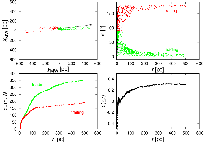
Figure 2: Hyades: (upper left:) Shown is the spatial distribution of the members of the Hyades (black), the leading tidal arm (green) and the trailing tidal arm (red) from Jerabkova et al. (2021). The coordinates $x_{\mathrm{MW}}$ and $y_{\mathrm{MW}}$ refer to a non-rotating rest frame of the Milky Way with a shifted origin where the position of the Sun lies at (0,0). The positive $x$-axis points towards the Galactic centre, the positive $y$-axis towards Galactic rotation. The arrow indicates the motion of the star cluster centre in the Galactic rest frame. (upper right:) Shown are the positions of cluster and tidal tidal members in polar coordinates calculated as described in Sect. 2. (lower left:) Radial cumulative distribution of the number of stars in the leading and trailing tidal arm of the Hyades (lower right:) Radial cumulative evolution of the normalised asymmetry (Eq. 1) considering tidal tail stars with a distance to the cluster centre smaller or equal to $r$.

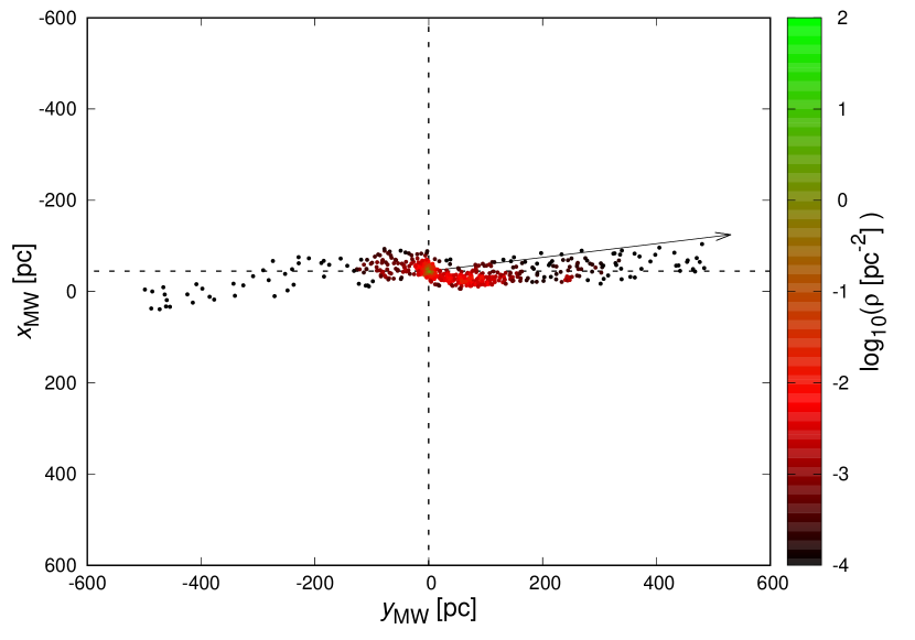
Figure 3: Surface number density of stars of the Hyades (cluster plus both tidal arms). Each dot represents one star. The local number density is calculated with the $6$th-nearest neighbour method (Casertano & Hut, 1985) and colour-coded. The black arrow indicates the velocity vector of the Hyades star cluster in the Galactic rest frame. The centre of the star cluster is located at the intersection of the two thin dashed lines.

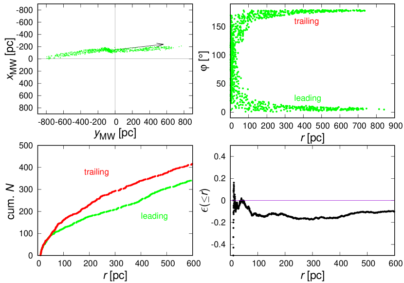
Figure 4: Praesepe from Jerabkova et al. (in prep.): Similar to Fig. 2.

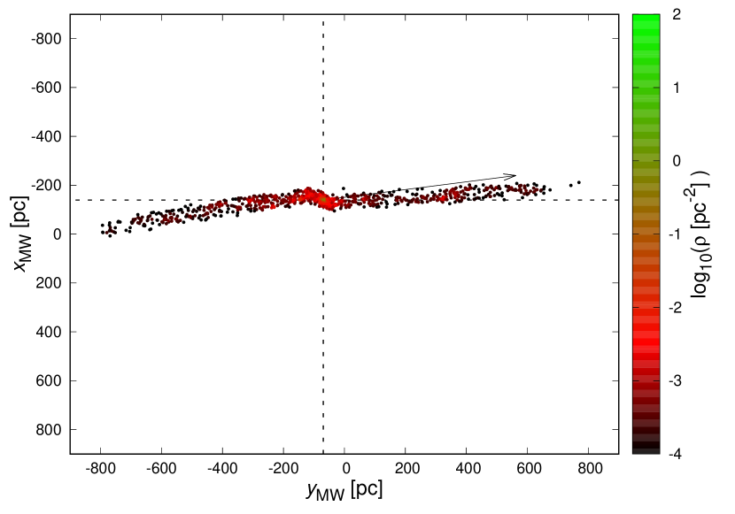
Figure 5: Praesepe: Similar to Fig. 3.

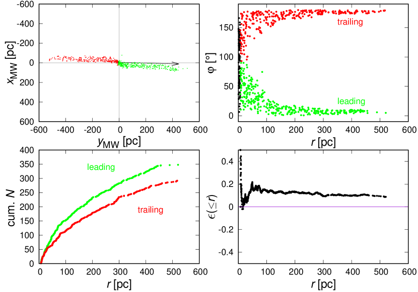
Figure 6: Coma Berenices from Jerabkova et al. (in prep.): Similar to Fig. 2.

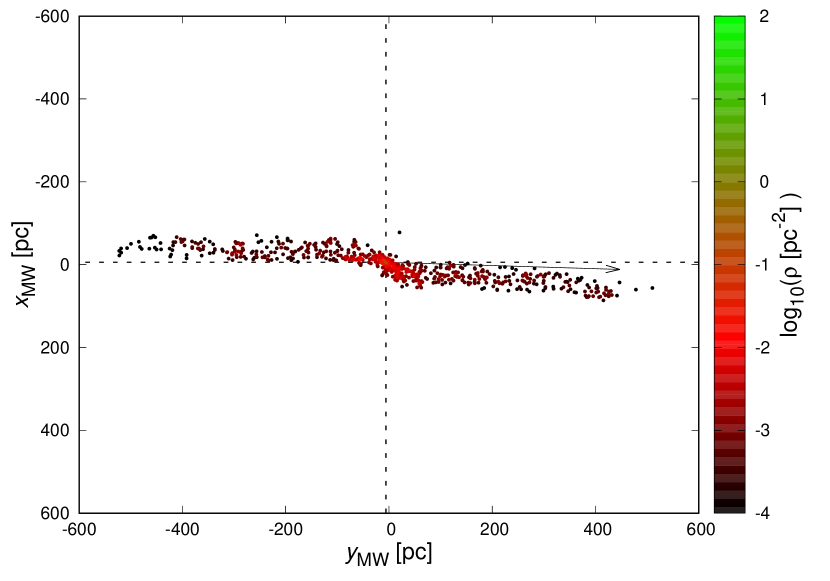
Figure 7: Coma Berenices: Similar to Fig. 3.

Figure 8: NGC 752 from Beccari et al. (2022): Similar to Fig. 2.

4 Monte Carlo simulations

In order to compare the observed asymmetries of tidal tails with the degree of asymmetry due to the stochastic evaporation of stars from star clusters embedded in a Galactic tidal field, a large number of test particle integrations are performed in the Galactic gravitational potential.

4.1 Numerical model

In the simulations a star cluster is set up as a Plummer phase-space distribution (Plummer, 1911; Aarseth et al., 1974) with initial parameters $b_{\mathrm{Pl}}$ being the Plummer radius and the total mass, $M_{\mathrm{Pl}}$. The centre of mass of the model, $\@vec{r}_{\mathrm{Pl}}$, moves in a Galactic potential as given in Allen & Santillan (1991). The orbit of each stellar test particle is integrated in both gravitational fields, the Plummer potential as the gravitational proxy of the star cluster and the full Galactic gravitational potential. Thus, the equations of motion of the star $i$ and of the cluster model are

$$\@vec{a}_{i}=-\nabla\Phi_{\mathrm{Pl}}-\nabla\Phi_{\mathrm{MW}}\,,$$ (2)

$$\@vec{a}_{\mathrm{Pl}}=-\nabla\Phi_{\mathrm{MW}}\,.$$ (3)

The test particles are distributed in the model cluster potential according to the Plummer phase-space distribution function and are integrated in time in the static Galactic potential and a static Plummer potential, whose origin is integrated as a test particle in the Galactic potential. In a self-gravitating system those particles evaporate from the cluster which gained sufficient energy by energy redistribution between the gravitationally interacting particles to exceed the binding energy to the cluster. In the model cluster all particles are treated as test particles and are integrated in a static potential without gravitational interaction between the particles. As energy redistribution does not occur in this model the evaporation process is simulated as follows: If the Plummer sphere were set up in isolation all particles had negative energy and were bound to the cluster. As the model cluster is positioned in the Galactic external potential the combined potential is lowered in two opposite points on the intersecting line defined by the Galactic origin and the cluster centre, being the Lagrange points. As a consequence, a fraction of the initial set of stars have positive energy with respect to the Lagrange points and lead to a continuous stream of escaping stars across the clusters’s tidal threshold (or práh according to Kroupa et al. 2022), with individual escape time scales up to a Hubble time. This method has been successfully tested in Fukushige & Heggie (2000).

The aim in this work is to quantify the expected distribution of the asymmetry between both tidal tails for the observed total number of tidal tail members due to stochastic evaporation through the Lagrange points. As not all test particles escape from the star cluster into the tidal arms a few test runs are required to calibrate the total number of test particles, such that the number of escaped stars is nearly equal to the observed number of tidal tail members.

As the stellar test particles are performing many revolutions around the star cluster centre before evaporating into the Galactic tidal field, the equations of motion are integrated with a time-symmetric Hermite method (Kokubo et al., 1998). The expressions of the accelerations and the corresponding time derivatives are listed in App. A for completeness.

As the total mass of the Plummer model is constant during the simulation, models with minimum and maximum star cluster mass are calculated in order to enclose the mass loss of real star clusters. Röser et al. (2011) estimated an initial stellar mass of the Hyades of 1100 $M_{\sun}$ and determined a current stellar mass gravitationally bound within the tidal radius of 275 $M_{\sun}$. Therefore, in the minimum model the mass of the Plummer sphere is given by the current stellar mass of the star cluster (Table 1), in the maximum model the mass of the Plummer sphere is set to four times the current stellar mass. The Plummer parameter, $b_{\mathrm{Pl}}$, is identical in both models.

Furthermore, these two models also take into account the possible range of tidal radii: a minimum model (current mass) with the smallest tidal radius and a maximum model (here 4x the current mass) with a plausible maximum tidal radius.

The orbits of the four star clusters are integrated backwards in time over their assumed life time from their current position (Table 1) to their location of formation. At this position 1000 randomly created Plummer models are set up for each maximum and minimum cluster. Each configuration is integrated forward in time over the assumed age of the respective star cluster. Finally all particles outside the tidal radius are assigned to their corresponding tidal arm using the method described in Sect. 2 and the normalised asymmetry, $\epsilon$, is calculated.

4.2 Statistical asymmetry

The numerically obtained distribution of the normalised asymmetry of all four star clusters is shown by the histograms in Fig. 9 for the minimum models and in Fig. 10 for the maximum models. The solid curves show the best-fitting Gaussian function. The vertical line marks the observed asymmetry (Table 1). The resulting mean asymmetry, $\mu$, and the dispersion, $\sigma$, of the Gaussian fits are listed in Table 2. In the last column in Table 2 the observed asymmetry is tabulated in units of the respective model dispersion. For example, in the case of the maximum model the observed asymmetry of the Praesepe cluster is a 1.7 $\sigma$ event.

Dispersion and mean value of the minimum and maximum are in good agreement. It can be concluded that the mass of the Plummer model has only a small influence. In the case of the Praesepe, the Coma Berenices and the NGC 752 star cluster the observed asymmetries have a probability less than 3 $\sigma$ and can be interpreted as pure statistical events. But, if the observed asymmetric tidal tails of the Hyades were solely the result of stochastic evaporation, then the asymmetry would be at least a 6.7 $\sigma$ event.

Figure 9: Monte Carlo results for the minimum model: Shown is the normalised distribution of the asymmetry in the Monte Carlo simulations for each star cluster model. The solid curve is the best-fitting Gaussian distribution function. The vertical solid line marks the observed value.

Figure 10: Similar to analysis as in Fig. 9 but for the maximum model.

Cluster	$\mu$	$\sigma$	$|x_{\mathrm{obs}}-\mu|$
Hyades (min)	-0.0088	0.042	7.3 $\sigma$
Hyades (max)	-0.0086	0.046	6.7 $\sigma$
Hyades (theo.)	0	0.043	6.9 $\sigma$
Praesepe (min)	-0.0163	0.036	-1.7 $\sigma$
Praesepe (max)	-0.0142	0.037	-1.7 $\sigma$
Praesepe (theo.)	0	0.035	-2.2 $\sigma$
Coma Berenices (min)	-0.0091	0.041	2.4 $\sigma$
Coma Berenices (max)	-0.0092	0.040	2.4 $\sigma$
Coma Berenices (theo.)	0	0.040	2.2 $\sigma$
NGC 752 (min)	-0.0052	0.055	1.6 $\sigma$
NGC 752 (max)	-0.0046	0.056	1.6 $\sigma$
NGC 752 (theo.)	0	0.058	1.6 $\sigma$

Table 2: Parameter of Gaussian fits of the asymmetry distribution of the different Monte Carlo models.

5 Theoretical considerations

In this section a theoretical stochastic evaporation model is developed and compared with the results of the numerical models of Sect. 4.

5.1 Theoretical distribution function, $f(\epsilon)$, of the asymmetry

The evaporation of a star into one of the tidal tails can be treated as a Bernoulli-experiment. Let $p_{\mathrm{l}}$ be the probability for a star to end up in the leading tail, $(1-p_{\mathrm{l}})$ the probability to end up in the trailing tail. For a total number $n$ of tidal tail members the probability that $n_{\mathrm{l}}$ stars are located in the leading arm is given by a binomial distribution

$$b_{n}(n_{\mathrm{l}})=\binom{n}{n_{\mathrm{l}}}p_{\mathrm{l}}^{n_{\mathrm{l}}}(1-p_{\mathrm{l}})^{n-n_{\mathrm{l}}}\,,$$ (4)

with an expectation value of $\mathrm{E}(n_{\mathrm{l}})=np_{\mathrm{l}}$ and a variance $\mathrm{Var}(n_{\mathrm{l}})=np_{\mathrm{l}}(1-p_{\mathrm{l}})$.

According to the theorem by de Moivre-Laplace, the binomial distribution converges against the Gaussian distribution,

$$g(n_{\mathrm{l}})=\frac{1}{\sqrt{2\pi\sigma_{\mathrm{l}}^{2}}}e^{-\frac{(n_{\mathrm{l}}-\mu_{\mathrm{l}})^{2}}{2\sigma_{\mathrm{l}}^{2}}}\,,$$ (5)

for increasing $n_{\mathrm{l}}$ with an expectation value $\mathrm{E}(n_{\mathrm{l}})=\mu_{\mathrm{l}}=np_{\mathrm{l}}$ and a variance $\mathrm{Var}(n_{\mathrm{l}})=\sigma_{\mathrm{l}}^{2}=np_{\mathrm{l}}(1-p_{\mathrm{l}})$.

The normalised asymmetry, $\epsilon$, is related to the number of members of the leading tail, $n_{\mathrm{l}}$, by

$$\epsilon=\frac{n_{\mathrm{l}}-n_{\mathrm{t}}}{n}=\frac{2n_{\mathrm{l}}}{n}-1\,.$$ (6)

The relation between the distribution function of the normalised asymmetry, $f(\epsilon)$, and the distribution of the member number of stars in the leading tail, $g(n_{\mathrm{l}})$, is given by

$$f(\epsilon)\;d\epsilon=g(n_{\mathrm{l}})\;dn_{\mathrm{l}}\,.$$ (7)

The distribution function of the asymmetry can then be calculated by

$$f(\epsilon)=g(n_{\mathrm{l}}(\epsilon))\left|\frac{dn_{\mathrm{l}}}{d\epsilon}(\epsilon)\right|=\frac{1}{\sqrt{2\pi\sigma_{\epsilon}^{2}}}e^{-\frac{\left(\epsilon-\mu_{\epsilon}\right)^{2}}{2\sigma_{\mathrm{\epsilon}}^{2}}}\,,$$ (8)

with $dn_{\mathrm{l}}/d\epsilon$ following from Eq. (6) and

$$\sigma_{\epsilon}^{2}=\frac{4\sigma_{\mathrm{l}}^{2}}{n^{2}}=\frac{4p_{\mathrm{l}}(1-p_{\mathrm{l}})}{n}\,,$$ (9)

and

$$\mu_{\epsilon}=\frac{2\mu_{\mathrm{l}}}{n}-1=2p_{\mathrm{l}}-1\,.$$ (10)

5.2 Symmetric evaporation

In the case of a symmetric population of the tidal tails, the evaporation probabilities into both arms are identical, $p_{\mathrm{l}}=p_{\mathrm{t}}=\frac{1}{2}$. The expectation value and the variance are

$$\mu_{\epsilon}=0\;\;\;,\;\;\;\sigma_{\epsilon}=\frac{1}{\sqrt{n}}\,.$$ (11)

For all four clusters the theoretically expected asymmetry due to stochastic evaporation, if the tidal tails are symmetrically populated, is listed in Table 2. It can be seen that in all four cases the theoretical values are close to the numerically obtained ones.

5.3 Asymmetric evaporation

Now, consider the case that the evaporation and the distribution processes within the vicinity of the star cluster into the tidal arms were asymmetric. According to Eq. 10 the expectation value of the asymmetry, $\mu_{\epsilon}$, increases, that is, more stars evaporate into the leading arm than into the trailing arm, if the population probability, $p_{\mathrm{l}}$, of the leading arm increases.

For a given observed asymmetry, $\epsilon_{\mathrm{obs}}$, the probability of this event can be calculated as multiples, $k$, of the dispersion for the assumed evaporation probability $p_{\mathrm{l}}$,

$$k=\frac{\epsilon_{\mathrm{obs}}-\mu_{\epsilon}(p_{\mathrm{l}})}{\sigma_{\epsilon}(p_{\mathrm{l}})}=\frac{\sqrt{n}(\epsilon_{\mathrm{obs}}-2p_{\mathrm{l}}+1)}{2\sqrt{p_{\mathrm{l}}(1-p_{\mathrm{l}})}}\;.$$ (12)

Fig. 11 shows this function for all four star clusters. The vertical dashed line marks the case of symmetrically populated tidal tails. For example, the Hyades have an observed asymmetry of $\epsilon_{\mathrm{obs}}=0.298$ (Table 1). In the case of a symmetric evaporation, $p_{\mathrm{l}}=\frac{1}{2}$, the theoretical dispersion is $\sigma=0.043$. Thus, the probabillity of this event is 0.298/0.043 = 6.9 $\sigma$. This point is marked in Fig. 11 by the intersection of the solid line labeled with Hyades and the vertical dashed line.

On the other hand, in order to increase the event probability (decreasing $k$) the probability of evaporation into the leading arm needs to be increased. For given $k$, Eq. (12) can be solved for the required evaporation probability, $p_{\mathrm{l}}$, into the leading arm. The emerging quadratic equation leads to two solutions of $p_{\mathrm{l}}$,

$$p_{1,2}=-\frac{a}{2}\pm\sqrt{\left(\frac{a}{2}\right)^{2}-b}\,,$$ (13)

where

$$a=-\frac{k^{2}+n(\epsilon_{\mathrm{obs}}+1)}{k^{2}+n}\;\;\;\mathrm{and}\;\;\;b=\frac{n(\epsilon_{\mathrm{obs}}+1)^{2}}{4k^{2}+4n}\,.$$ (14)

If the observed asymmetry of the Hyades should be a 3 $\sigma$ event then an evaporation probability into the leading arm of approximately $p_{\mathrm{l}}=0.585$ is required.

Figure 11: Shown is the probability of the observed asymmetry of all four star clusters as a multiple of the dispersion in dependence of the assumed evaporation probability into the leading arm, $p_{\mathrm{l}}$. See Sect. 5.3 for details.

6 Discussion and Conclusions

The common assumption that both tidal tails of star clusters, moving on nearly circular obits around the Galactic centre, evolve equally has recently faced a challenge as the analysis of Gaia data reveal asymmetries in the tidal tails of four nearby open star clusters.

Because the evaporation of stars can be treated as a stochastic process the normalised difference of the number of member stars of both tails should follow a distribution function. This distribution has been quantified here by use of Monte Carlo simulations of test particle configurations integrated in the full Galactic potential and compared with a theoretical approach. It emerges that the theoretical and numerical results agree with each other.

Comparing the individual distribution functions of the asymmetry with the observed ones, it can be concluded that the observed asymmetry of Praesepe, Coma Berenices and NGC 752 might be the result of the stochastic nature of the evaporation of stars through both Lagrange points. On the other hand, the asymmetry of the Hyades is a 6.7 $\sigma$ event. In order to interpret the asymmetry as a 3 $\sigma$ event, asymmetric evaporation probabilities into the leading arm of 58.5% and into the trailing arm of 41.5% are required.

It might be speculated that external effects might lead to an additional broadening of the distribution function of the asymmetry. Assuming a different value for the Galactic rotational velocity or a different position of the Sun than used in this work might not lead to a larger scatter as the 50/50% evaporation probabilities at both Lagrange points are not expected to vary in an almost flat rotation curve.

A stronger effect on the asymmetry of the tidal tails might be due to local deviations from a logarithmic potential (as required in the case of a flat rotation curve). Such local variations can be a result of an interaction with a Galactic bar or spiral arms (cf. Bonaca et al., 2020; Pearson et al., 2017). How strong this effect will be can be hardly estimated and will be explored in further numerical studies. However, the main result here, that the pure evaporation of stars through the Lagrange points is basically a simple Bernoulli process, remains solid.

If the asymmetric evaporation probabilities have an internal origin, then larger asymmetries in the star cluster potential and the kinematics of the evaporation process is required than Newtonian dynamics can provide (Kroupa et al., 2022). On the other hand the asymmetry might be due to an external perturbation, for example through the encounter with a molecular cloud (Jerabkova et al., 2021). However, the detailed analysis of the asymmetry in the tidal tails of the Hyades reveals that the process leading to the asymmetry must affect both arms equally in terms of the qualitative structure. The bending of the radial number distributions occur at the same distance to the star cluster but with different strength (Fig. 2, lower left panel). If an encounter with an external object had occurred on one side of the star cluster then it is expected that more than only the total number of tidal tail members is reduced. Instead, the functional form of the cumulative number distribution in both arms would be completely different and rapid changes of the slopes of the cumulative number distribution would not be expected to occur at the same distance from the star cluster centre in both tidal tails on opposite sites of the star cluster as is observed in the tidal tails of the Hyades (Fig. 2, lower left panel).

Appendix A Hermite formulae for the Allen-Santillan potential

The total Galactic gravitational field has contributions from three components: Galactic bulge, disk and halo. The rotationally symmetric gravitational potentials are taken from Allen & Santillan (1991). The time-symmetric Hermite integrator from Kokubo et al. (1998) requires the accelerations $\@vec{a}$ and their time derivatives $\@vec{j}=\@vec{\dot{a}}$ and are listed below. The following notations are used: $\@vec{r}=(x,y,z)$, $\bm{\rho}=(x,y,0)$, $\@vec{z}=(0,0,z)$, $\@vec{\dot{r}}=\@vec{v}=(\dot{x},\dot{y},\dot{z})$, $\bm{\dot{\rho}}=(\dot{x},\dot{y},0)$, $\@vec{\dot{z}}=(0,0,\dot{z})$.

$$\Phi(\rho,z)=\Phi_{\mathrm{bulge}}(\rho,z)+\Phi_{\mathrm{disk}}(\rho,z)+\Phi_{\mathrm{halo}}(\rho,z)$$ (15)

$$\@vec{a}=\@vec{a}_{\mathrm{bulge}}+\@vec{a}_{\mathrm{disk}}+\@vec{a}_{\mathrm{halo}}=-\nabla\Phi_{\mathrm{bulge}}-\nabla\Phi_{\mathrm{disk}}-\nabla\Phi_{\mathrm{halo}}$$ (16)

$$\@vec{j}=\@vec{j}_{\mathrm{bulge}}+\@vec{j}_{\mathrm{disk}}+\@vec{j}_{\mathrm{halo}}$$ (17)

A.1 bulge

$$\Phi_{\mathrm{bulge}}(\rho,z)=-GM_{1}\frac{1}{\sqrt{\rho^{2}+z^{2}+b_{1}^{2}}}$$ (18)

$$\@vec{a}_{\mathrm{bulge}}=-GM_{1}\left(\rho^{2}+z^{2}+b_{1}^{2}\right)^{-\frac{3}{2}}\@vec{r}$$ (19)

$$\@vec{j}_{\mathrm{bulge}}=-GM_{1}\left(\rho^{2}+z^{2}+b_{1}^{2}\right)^{-\frac{3}{2}}\left(\@vec{v}-3\frac{{\@vec{\dot{r}}}\bullet\@vec{r}}{\rho^{2}+z^{2}+b_{1}^{2}}\@vec{r}\right)$$ (20)

A.2 disk

$$\Phi_{\mathrm{disk}}(\rho,z)=-GM_{2}\frac{1}{\sqrt{\rho^{2}+\left(a_{2}+\sqrt{z^{2}+b_{2}^{2}}\right)^{2}}}$$ (21)

$$\@vec{a}=-GM_{2}\left(\rho^{2}+\left(a_{2}+\left(z^{2}+b_{2}^{2}\right)^{\frac{1}{2}}\right)^{2}\right)^{-\frac{3}{2}}$$ (22)

$$\left(\bm{\rho}+\left(1+\frac{a_{2}}{\sqrt{z^{2}+b_{2}^{2}}}\right)\@vec{z}\right)$$ (23)

$$\@vec{j}=3M_{2}G\left(\rho^{2}+\left(a_{2}+\left(z^{2}+b_{2}^{2}\right)^{\frac{1}{2}}\right)^{2}\right)^{-\frac{5}{2}}\cdot\hfill\hfill$$ (24)

$$\left(\bm{\rho}\bullet\dot{\bm{\rho}}+\left(1+\frac{a_{2}}{\sqrt{z^{2}+b_{2}^{2}}}\right)\@vec{z}\bullet\dot{\@vec{z}}\right)\left(\bm{\rho}+\left(1+\frac{a_{2}}{\sqrt{z^{2}+b_{2}^{2}}}\right)\@vec{z}\right)$$ (25)

$$-M_{2}G\left(\rho^{2}+\left(a_{2}+\left(z^{2}+b_{2}^{2}\right)^{\frac{1}{2}}\right)^{2}\right)^{-\frac{3}{2}}\cdot$$ (26)

$$\left(\dot{\bm{\rho}}-\frac{a_{2}\@vec{z}\bullet\dot{\@vec{z}}}{\left(z^{2}+b_{2}^{2}\right)^{\frac{3}{2}}}\@vec{z}+\left(1+\frac{a_{2}}{\sqrt{z^{2}+b_{2}^{2}}}\right)\dot{\@vec{z}}\right)$$ (27)

A.3 halo

$$\Phi_{\mathrm{halo}}=-\frac{GM_{\mathrm{halo}}(\leq r)}{r}-\frac{GM_{3}}{(\gamma-1)a_{3}}\left[-\frac{\gamma-1}{1+\left(\frac{r}{a_{3}}\right)^{\gamma-1}}+\ln\left(1+\left(\frac{r}{a_{3}}\right)^{\gamma-1}\right)\right]_{r}^{100}\,,$$ (28)

where

$$M(\leq r)=\frac{M_{3}\left(\frac{r}{a_{3}}\right)^{\gamma}}{1+\left(\frac{r}{a_{3}}\right)^{\gamma-1}}$$ (29)

is the total halo mass within the Galactocentric radius $r$.

$$\@vec{a}_{\mathrm{halo}}=-\frac{GM(\leq r)}{r^{3}}\@vec{r}$$ (30)

$$\@vec{j}_{\mathrm{halo}}=-\frac{GM(r)}{r^{3}}\left(\@vec{v}-\frac{\@vec{r}\bullet\@vec{v}}{r^{2}}\left(\gamma-3-\frac{(\gamma-1)\left(\frac{r}{a_{3}}\right)^{\gamma-1}}{1+\left(\frac{r}{a_{3}}\right)^{\gamma-1}}\right)\@vec{r}\right)$$ (31)

A.4 Units and parameters

In Allen & Santillan (1991) the spatial variables of the potential have the unit kpc, the velocity the unit 10 km s^-1 and the potential the unit 100 km² s^-2. Thus, the accelerations needs to be multiplied by 0.104572 in order to have the unit pc Myr^-2 and their time derivatives, $\@vec{j}$, by $1.06936\times 10^{-3}$ to have the unit pc Myr^-3. The mass has the unit $2.3262\times 10^{7}\,M_{\sun}$ and is scaled such that the gravitational constant is $G=1$. The parameters of the potentials are summarised in Table 3.

component	parameter
bulge	$M_{1}$ = 606.0
bulge	$b_{1}$ = 0.3873
disk	$M_{2}$ = 3690.0
disk	$a_{2}$ = 5.3178
disk	$b_{2}$ = 0.2500
halo	$M_{3}$ = 4615.0
halo	$a_{3}$ = 12.0
halo	$\gamma$ = 2.02

Table 3: Parameters of the potential used in this work.

A.5 Hermite formulae for the Plummer sphere

$$\Phi_{\mathrm{Pl}}(r)=-GM_{\mathrm{Pl}}\frac{1}{\sqrt{r^{2}+b_{\mathrm{Pl}}^{2}}}$$ (32)

$$\@vec{a}_{\mathrm{Pl}}=-GM_{\mathrm{Pl}}\left(r^{2}+b_{\mathrm{Pl}}^{2}\right)^{-\frac{3}{2}}\@vec{r}$$ (33)

$$\@vec{j}_{\mathrm{Pl}}=-GM_{\mathrm{Pl}}\left(r^{2}+b_{\mathrm{Pl}}^{2}\right)^{-\frac{3}{2}}\left(\@vec{v}-3\frac{{\@vec{\dot{r}}}\bullet\@vec{r}}{r^{2}+b_{\mathrm{Pl}}^{2}}\@vec{r}\right)$$ (34)

References

- Aarseth (1999) Aarseth, S. J. 1999, PASP, 111, 1333
- Aarseth (2003) Aarseth, S. J. 2003, Gravitational N-Body Simulations (Gravitational N-Body Simulations, by Sverre J. Aarseth, pp. 430. ISBN 0521432723. Cambridge, UK: Cambridge University Press, November 2003.)
- Aarseth et al. (1974) Aarseth, S. J., Henon, M., & Wielen, R. 1974, A&A, 37, 183
- Allen & Santillan (1991) Allen, C. & Santillan, A. 1991, Revista Mexicana de Astronomia y Astrofisica, 22, 255
- Allen et al. (2007) Allen, L., Megeath, S. T., Gutermuth, R., et al. 2007, Protostars and Planets V, 361
- Baumgardt & Kroupa (2007) Baumgardt, H. & Kroupa, P. 2007, MNRAS, 380, 1589
- Beccari et al. (2022) Beccari, G., Jerabkova, T., Boffin, H. M. J., et al. 2022, in preparation
- Boffin et al. (2022) Boffin, H. M. J., Jerabkova, T., Beccari, G., & Wang, L. 2022, MNRAS, 514, 3579
- Bonaca et al. (2020) Bonaca, A., Pearson, S., Price-Whelan, A. M., et al. 2020, ApJ, 889, 70
- Casertano & Hut (1985) Casertano, S. & Hut, P. 1985, ApJ, 298, 80
- Fukushige & Heggie (2000) Fukushige, T. & Heggie, D. C. 2000, MNRAS, 318, 753
- Jerabkova et al. (2021) Jerabkova, T., Boffin, H. M. J., Beccari, G., et al. 2021, A&A, 647, A137
- Jerabkova et al. (in prep.) Jerabkova, T., Boffin, H. M. J., Beccari, G., et al. in prep., in preparation
- Kokubo et al. (1998) Kokubo, E., Yoshinaga, K., & Makino, J. 1998, MNRAS, 297, 1067
- Kroupa et al. (2022) Kroupa, P., Jerabkova, T., Thies, I., et al. 2022, MNRAS, 517, 3613
- Küpper et al. (2010) Küpper, A. H. W., Kroupa, P., Baumgardt, H., & Heggie, D. C. 2010, MNRAS, 401, 105
- Lada & Lada (2003) Lada, C. J. & Lada, E. A. 2003, ARA&A, 41, 57
- Oh & Kroupa (2016) Oh, S. & Kroupa, P. 2016, A&A, 590, A107
- Pearson et al. (2017) Pearson, S., Price-Whelan, A. M., & Johnston, K. V. 2017, Nature Astronomy, 1, 633
- Pflamm-Altenburg & Kroupa (2006) Pflamm-Altenburg, J. & Kroupa, P. 2006, MNRAS, 373, 295
- Plummer (1911) Plummer, H. C. 1911, MNRAS, 71, 460
- Poveda et al. (1967) Poveda, A., Ruiz, J., & Allen, C. 1967, Boletin de los Observatorios Tonantzintla y Tacubaya, 4, 86
- Röser et al. (2011) Röser, S., Schilbach, E., Piskunov, A. E., Kharchenko, N. V., & Scholz, R. D. 2011, A&A, 531, A92