HyperReel: High-Fidelity 6-DoF Video with Ray-Conditioned Sampling

Abstract

Volumetric scene representations enable photorealistic view synthesis for static scenes and form the basis of several existing 6-DoF video techniques. However, the volume rendering procedures that drive these representations necessitate careful trade-offs in terms of quality, rendering speed, and memory efficiency. In particular, existing methods fail to simultaneously achieve real-time performance, small memory footprint, and high-quality rendering for challenging real-world scenes. To address these issues, we present HyperReel — a novel 6-DoF video representation. The two core components of HyperReel are: (1) a ray-conditioned sample prediction network that enables high-fidelity, high frame rate rendering at high resolutions and (2) a compact and memory-efficient dynamic volume representation. Our 6-DoF video pipeline achieves the best performance compared to prior and contemporary approaches in terms of visual quality with small memory requirements, while also rendering at up to 18 frames-per-second at megapixel resolution without any custom CUDA code.

¹Carnegie Mellon University ²University of Maryland ³Reality Labs Research ⁴Meta

https://hyperreel.github.io

Dynamic 6-DoF rendering

 
Static 6-DoF rendering

Figure 1: HyperReel: A novel 6-DoF video representation. HyperReel converts synchronized multi-view video streams into a high-fidelity, memory efficient scene representation that can be rendered from novel views and time steps at interactive rates. HyperReel’s combination of high rendering quality, speed, and compactness sets it apart from existing 6-DoF video representations. The upper two rows show 6-DoF (i.e., varying viewpoint and viewing orientation) rendering of dynamic scenes [9, 48]; the lower two of static scenes [65, 62].

1 Introduction

Six–Degrees-of-Freedom (6-DoF) videos allow for free exploration of an environment by giving the users the ability to change their head position (3 degrees of freedom) and orientation (3 degrees of freedom). As such, 6-DoF videos offer immersive experiences with many exciting applications in AR/VR. The underlying methodology that drives 6-DoF video is view synthesis: the process of rendering new, unobserved views of an environment—static or dynamic—from a set of posed images or videos. Volumetric scene representations such as neural radiance fields [32] and instant neural graphics primitives [33] have recently made great strides toward photorealistic view synthesis for static scenes.

While several recent works build dynamic view synthesis pipelines on top of these volumetric representations [68, 25, 15, 37, 24], it remains a challenging task to create a 6-DoF video format that can achieve high quality, fast rendering, and a small memory footprint (even given many synchronized video streams from multi-view camera rigs [48, 39, 9]). Existing approaches that attempt to create memory-efficient 6-DoF video can take nearly a minute to render a single megapixel image [24]. Works that target rendering speed and represent dynamic volumes directly with 3D textures require gigabytes of storage even for short video clips [61]. While other volumetric methods achieve memory efficiency and speed by leveraging sparse or compressed volume storage for static scenes [33, 11], only contemporary work [23, 53] addresses the extension of these approaches to dynamic scenes. Moreover, all of the above representations struggle to capture highly view-dependent appearance, such as reflections and refractions caused by non-planar surfaces.

In this paper, we present HyperReel, a novel 6-DoF video representation that achieves state-of-the-art quality while being memory efficient and real-time renderable at high resolution. The first ingredient of our approach is a novel ray-conditioned sample prediction network that predicts sparse point samples for volume rendering. In contrast to existing static view synthesis methods that use sample networks [34, 21], our design is unique in that it both (1) accelerates volume rendering and at the same time (2) improves rendering quality for challenging view-dependent scenes.

Second, we introduce a memory-efficient dynamic volume representation that achieves a high compression rate by exploiting the spatio-temporal redundancy of a dynamic scene. Specifically, we extend Tensorial Radiance Fields [11] to compactly represent a set of volumetric keyframes, and capture intermediate frames with trainable scene flow.

The combination of these two techniques comprises our high-fidelity 6-DoF video representation, HyperReel. We validate the individual components of our approach and our representation as a whole with comparisons to state-of-the-art sampling network-based approaches for static scenes as well as 6-DoF video representations for dynamic scenes. Not only does HyperReel outperform these existing works, but it also provides high-quality renderings for scenes with challenging non-Lambertian appearances. Our system renders at up to 18 frames-per-second at megapixel resolution without using any custom CUDA code.

The contributions of our work include the following:

1. A novel sample prediction network for volumetric view synthesis that accelerates volume rendering and accurately represents complex view-dependent effects.

2. A memory-efficient dynamic volume representation that compactly represents a dynamic scene.

3. HyperReel, a 6-DoF video representation that achieves a desirable trade-off between speed, quality, and memory, while rendering in real time at high resolutions.

2 Related Work

Novel View Synthesis

Novel-view synthesis is the process of rendering new views of a scene given a set of input posed images. Classical image-based rendering techniques use approximate scene geometry to reproject and blend source image content onto novel views [10, 50, 41]. Recent works leverage the power of deep learning and neural fields [69] to improve image-based rendering from both structured (e.g., light fields [17, 22]) and unstructured data [7, 54]. Rather than performing image-based rendering, which requires storing the input images, another approach is to optimize some 3D scene representation augmented with appearance information [45]. Examples of such representations include point clouds [1, 44], voxel grids [29, 35, 51], meshes [46, 47], or layered representations like multi-plane [72, 31, 13] or multi-sphere images [2, 9].

Neural Radiance Fields

NeRFs are one such 3D scene representation for view synthesis [32] that parameterize the appearance and density of every point in 3D space with a multilayer perceptron (MLP). While NeRFs enable high-quality view synthesis at a small memory cost, they do not lend themselves to real-time rendering. To render the color of a ray from a NeRF, one must evaluate and integrate the color and opacity of many points along a ray—necessitating, in the case of NeRF, hundreds of MLP evaluations per pixel. Still, due to its impressive performance for static view synthesis, recent methods build on NeRFs in the quest for higher visual quality, more efficient training, and faster rendering speed [58, 16]. Several works improve the quality of NeRFs by accounting for finite pixels and apertures [5, 67], by enabling application to unbounded scenes [71, 6, 70], large scenes [57, 30] or by modifying the representation to allow for better reproduction of challenging view-dependent appearances like reflections and refractions [18, 59, 20, 8]. One can achieve significant training and inference speed improvements by replacing the deep multilayer perceptron with a feature voxel grid in combination with a small neural network [55, 33, 11] or no network at all [70, 19]. Several other works achieve both fast rendering and memory-efficient storage with tensor factorizations [11], learned appearance codebooks, or quantized volumetric features [56].

Adaptive Sampling for Neural Volume Rendering

Other works aim to improve the speed of volumetric representations by reducing the number of volume queries required to render a single ray. Approaches like DoNeRF [34], TermiNeRF [42], and AdaNeRF [21] learn weights for each segment along a ray as a function of the ray itself, and use these weights for adaptive evaluation of the underlying NeRF. In doing so, they can achieve near-real-time rendering. NeuSample [12] replaces the NeRF coarse network with a module that directly predicts the distance to each sample point along a ray. Methods like AutoInt [27], DIVeR [66], and neural light fields [4, 52, 26] learn integrated opacity and color along a small set of ray segments (or just one segment), requiring only a single network evaluation per segment. A key component of our framework is a flexible sampling network, which is among one of the few schemes that both accelerates volume rendering, and also improves volume rendering quality for challenging scenes.

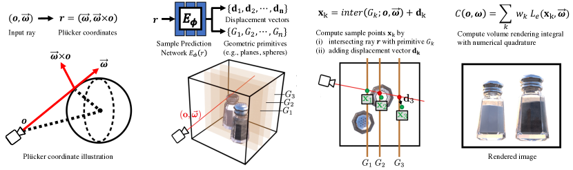
(a) Ray parameterization

(b) Sample prediction network

(c) Sample generation

(d) Volume rendering

Figure 2: Overview of HyperReel for static scenes. Given a set of images and camera poses, the training objective is to reconstruct the measured color associated with every ray. (a) For a ray originating at the camera origin $\mathbf{o}$ and traveling in direction $\vec{\boldsymbol{\omega}}$, we first reparameterize the ray using Plücker coordinates. (b) A network $E_{\phi}$ takes this ray as input and outputs the parameters for a set of geometric primitives $\{G_{k}\}$ (such as axis-aligned planes and spheres) and displacement vectors $\{\mathbf{d}_{k}\}$. (c) To generate sample points $\{\mathbf{x}_{k}\}$ for volume rendering, we compute the intersections between the ray and the geometric primitives, and add the displacement vectors to the results. (d) Finally, we perform volume rendering via Equation 2 to produce a pixel color and supervise training based on the corresponding observation.

6–Degrees-of-Freedom Video

6-DoF video is an emergent technology that allows users to explore new views within videos [45]. Systems for 6-DoF video [39] use multi-view camera rigs that capture a full 360-degree field of view and use variants of depth-based reprojection [49] for view synthesis at each frame of the video. Other methods optimize time-varying multi-sphere images (MSIs) [9, 2], which can provide better visual quality but at a higher training cost.

6-DoF from Monocular Captures

Due to the success of neural radiance fields for static view synthesis, many recent approaches attempt to extend volumetric scene representations to dynamic scenes. Several such works reconstruct 6-DoF video from single-view (i.e. monocular) RGB sequences [25, 15, 37, 28]. This is a highly under-constrained setting, which requires decoupling camera and object motion. The natural signal priors provided by neural radiance fields help during reconstruction. However, most methods typically rely on additional priors, such as off-the-shelf networks for predicting scene flow and geometry or depth from ToF cameras [68, 3]. Still, other approaches model the scene at different time steps as smoothly “warped” copies of some canonical frame [37, 43], which works best for small temporal windows and smooth object motion.

6-DoF from Multi-View Captures

Other methods, like ours, aim to produce 6-DoF video from multi-view camera rigs [29, 9, 24]. Despite the additional constraints provided by multiple cameras, this remains a challenging task; an ideal 6-DoF video format must simultaneously achieve high visual quality, rendering speed, and memory efficiency. Directly extending recent volumetric methods to dynamic scenes can achieve high quality and rendering speed [61], but at the cost of substantial memory requirements, potentially gigabytes of memory [70] for each video frame. Contemporary works such as StreamRF [23] and NeRFPlayer [53] design volumetric 6-DoF video representations that mitigate storage requirements but sacrifice either rendering speed or visual quality. On the other hand, our approach achieves both fast and high-quality 6-DoF video rendering while maintaining a small memory footprint.

3 Method

We start by considering the problem of optimizing a volumetric representation for static view synthesis. Volume representations like NeRF [32] model the density and appearance of a static scene at every point in the 3D space. More specifically, a function $F_{\boldsymbol{\theta}}:(\mathbf{x},\vec{\boldsymbol{\omega}})\rightarrow(L_{\text{e}}(\mathbf{x},\vec{\boldsymbol{\omega}}),\sigma(\mathbf{x}))$ maps position $\mathbf{x}$ and direction $\vec{\boldsymbol{\omega}}$ along a ray to a color $L_{\text{e}}(\mathbf{x},\vec{\boldsymbol{\omega}})$ and density $\sigma(\mathbf{x})$. Here, the trainable parameters $\boldsymbol{\theta}$ may be neural network weights, $N$-dimensional array entries, or a combination of both.

We can then render new views of a static scene with

$$C(\mathbf{o},\vec{\boldsymbol{\omega}})=\int_{t_{\text{n}}}^{t_{\text{f}}}\!\!\!\underbrace{T\!\left(\mathbf{o},\mathbf{x}_{t}\right)}_{\text{\scriptsize Transmittance}}\,\underbrace{\sigma\!\left(\mathbf{x}_{t}\right)}_{\text{\scriptsize Density}}\,\underbrace{L_{\text{e}}\!\left(\mathbf{x}_{t},\vec{\boldsymbol{\omega}}\right)}_{\text{\scriptsize Radiance}}\,\mathrm{d}t\text{,}$$ (1)

where $T\left(\mathbf{o},\mathbf{x}_{t}\right)$ denotes the transmittance from $\mathbf{o}$ to $\mathbf{x}_{t}$.

In practice, we can evaluate Equation 1 using numerical quadrature by taking many sample points along a given ray:

$$C(\mathbf{o},\vec{\boldsymbol{\omega}})\approx\sum_{k=1}^{N}w_{k}\,L_{\text{e}}\!\left(\mathbf{x}_{k},\vec{\boldsymbol{\omega}}\right)\text{,}$$ (2)

where the weights $w_{k}=\hat{T}\left(\mathbf{o},\mathbf{x}_{k}\right)(1-e^{-\sigma(\mathbf{x}_{k})\Delta\mathbf{x}_{k}})$ specify the contribution of each sample point’s color to the output.

3.1 Sample Networks for Volume Rendering

Most scenes consist of solid objects whose surfaces lie on a 2D manifold within the 3D scene volume. In this case, only a small set of sample points contributes to the rendered color for each ray. To accelerate volume rendering, we would like to query color and opacity only for points with non-zero $w_{k}$. While most volume representations use importance sampling and pruning schemes that help reduce sample counts, they often require hundreds or even thousands of queries per ray to produce accurate renderings [11, 33].

As shown in Figure 2, we use a feed-forward network to predict a set of sample locations $\mathbf{x}_{k}$. Specifically, we use a sample prediction network $E_{\boldsymbol{\phi}}:\left(\mathbf{o},\vec{\boldsymbol{\omega}}\right)\rightarrow\left(\mathbf{x}_{1},\dots,\mathbf{x}_{n}\right)$ that maps a ray $(\mathbf{o},\vec{\boldsymbol{\omega}})$ to the sample points $\mathbf{x}_{k}$ for volume rendering in Equation 2. We use either the two-plane parameterization [22] (for forward facing scenes) or the Plücker parameterization (for all other scenes) to represent the ray:

$$\mathbf{r}=\textit{Pl\"{u}cker}(\mathbf{o},\vec{\boldsymbol{\omega}})=\left(\vec{\boldsymbol{\omega}},\vec{\boldsymbol{\omega}}\times\mathbf{o}\right)\text{.}$$ (3)

While many designs for the sample prediction network $E_{\boldsymbol{\phi}}$ are possible, giving the network too much flexibility may negatively affect view synthesis quality. For example, if $\left(\mathbf{x}_{1},\dots,\mathbf{x}_{n}\right)$ are completely arbitrary points, then renderings may not appear to be multi-view-consistent.

To address this problem, we choose to predict the parameters of a set of geometric primitives $G_{1},\dots,G_{n}$ defined in the world coordinate frame, where the primitive parameters themselves are a function of the input ray. To get our sample points, we then intersect the ray with each primitive:

$$\!\!\!\!E_{\boldsymbol{\phi}}(\mathbf{o},\vec{\boldsymbol{\omega}}) =\left(G_{1},\dots,G_{n}\right)\,,$$ (4)

$$\!\!\!\!\left(\mathbf{x}_{1},\dots,\mathbf{x}_{n}\right) =\left(\textit{inter}(G_{1};\mathbf{o},\vec{\boldsymbol{\omega}}),\dots,\textit{inter}(G_{n};\mathbf{o},\vec{\boldsymbol{\omega}})\right)\!\text{.}$$ (5)

Above, $\textit{inter}(G_{k};\mathbf{o},\vec{\boldsymbol{\omega}})$ is a differentiable operation that intersects the ray with the primitive $G_{k}$. In all of our experiments, we use axis-aligned $z$-planes (for forward-facing scenes) or concentric spherical shells centered at the origin (for all other scenes) as our geometric primitives.

This approach is constrained in that it produces sample points that initially lie along the ray. Further, predicting primitives defined in world space makes the sample signal easier to interpolate. For example, if two distinct rays observe the same point in the scene, then the sample network needs only predict one primitive for both rays (i.e., defining a primitive that passes through the point). In contrast, existing works such as NeuSample [12], AdaNeRF [21], and TermiNeRF [42] predict distances or per-segment weights that do not have this property.

Flexible Sampling for Challenging Appearance.

To grant our samples additional flexibility to better represent challenging view-dependent appearance, we also predict a set of Tanh-activated per-sample-point offsets $\left(\mathbf{e}_{1},\dots,\mathbf{e}_{n}\right)$, as well as a set of scalar values $\left(\delta_{1},\dots,\delta_{n}\right)$. We convert these scalar values to weights with a sigmoid activation, i.e., $\left(\gamma(\delta_{1}),\dots,\gamma(\delta_{n})\right)$ where $\gamma$ is the sigmoid operator. Specifically, we have:

$$\left(\mathbf{d}_{1},\dots\mathbf{d}_{n}\right) =\left(\gamma(\delta_{1})\mathbf{e}_{1},\dots,\gamma(\delta_{n})\mathbf{e}_{n}\right)$$ (6)

$$\left(\mathbf{x}_{1},\dots\mathbf{x}_{n}\right) \leftarrow\left(\mathbf{x}_{1}+\mathbf{d}_{1},\dots,\mathbf{x}_{n}+\mathbf{d}_{n}\right)\text{,}$$ (7)

where we use $\left(\mathbf{d}_{1},\dots,\mathbf{d}_{n}\right)$ to denote the final displacement, or “point-offset” added to each point.

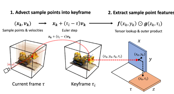
Figure 3: Extracting sample point appearance and opacity in the dynamic setting from our keyframe-based representation. (1) We first advect the sample points $\{\mathbf{x}_{k}\}$ at time $\tau$ into the nearest keyframe $\tau_{i}$, using velocities $\{\mathbf{v}_{k}\}$ from the sample prediction network. (2) We then query the outer products of space-time textures in order to produce per-sample-point appearance and opacity features, which are converted to colors/densities via Equation 10.

While the sample network outputs may appear to be over-parameterized and under-constrained, this is essential to achieve good-quality view synthesis. In particular, initializing the scalars $(\delta_{1},\dots,\delta_{n})$ to negative values, where the sigmoid is close to 0, and its gradient is small, implicitly discourages the network from unmasking the point offsets, while still allowing the network to use them as necessary.

In addition to enabling real-time rendering with low sample counts, one added benefit of our sample network architecture is the improved modeling of complex view-dependent appearance. For example, distorted refractions break epipolar geometry and appear to change the depth of the refracted content depending on the viewpoint. As illustrated in Figure 2, our sample network, on the other hand, has the flexibility to model sample points that warp depending on viewpoint, similar to flow-based models of scene appearance in IBR [36]

Existing works like Eikonal fields [8] can be considered a special case of this sample warping approach; they use physically derived Eikonal constraints to learn ray-conditional warp fields for refractive objects. Although our sample network is not guaranteed to be physically interpretable, it can handle both reflections and refractions. Further, it is far more efficient at inference time and does not require evaluating costly multi-step ODE solvers during rendering. See Figure 1 and our supplemental materials for additional results and comparisons on challenging view-dependent scenes.

3.2 Keyframe-Based Dynamic Volumes

So far, we have covered how to efficiently sample a 3D scene volume, but have not yet discussed how we represent the volume itself. In the static case, we use memory-efficient Tensorial Radiance Fields (TensoRF) approach (Section 3.2.1), and in the dynamic case we extend TensoRF to a keyframe-based dynamic volume representation (Section 3.2.2).

3.2.1 Representing 3D Volumes with TensoRF [11]

Recall that TensoRF factorizes a 3D volume as a set of outer products between functions of one or more spatial dimensions. Specifically, we can write the set of spherical harmonic coefficients $A\left(\mathbf{x}_{k}\right)$ capturing the appearance of a point $\mathbf{x}_{k}=(x_{k},y_{k},z_{k})$ as:

$$A\left(\mathbf{x}_{k}\right) =\mathcal{B}_{1}\!\left(\mathbf{f}_{1}(x_{k},y_{k})\odot\mathbf{g}_{1}(z_{k})\right)$$

$$+\mathcal{B}_{2}\!\left(\mathbf{f}_{2}(x_{k},z_{k})\odot\mathbf{g}_{2}(y_{k})\right)$$ (8)

$$+\mathcal{B}_{3}\!\left(\mathbf{f}_{3}(y_{k},z_{k})\odot\mathbf{g}_{3}(x_{k})\right)\text{.}$$

Above, $\mathbf{f}_{j}$ and $\mathbf{g}_{j}$ are vector-valued functions with output dimension $M$, and ‘$\odot$’ is an element-wise product. In the original TensoRF work [11], the functions $\mathbf{f}_{j}$ and $\mathbf{g}_{j}$ are discretized into $M$ different 2D and and 1D arrays, respectively.

Further, $\mathcal{B}_{j}$ denote linear transforms that map the products of $\mathbf{f}_{j}$ and $\mathbf{g}_{j}$ to spherical harmonic coefficients. The color $L_{e}(\mathbf{x}_{k},\vec{\boldsymbol{\omega}})$ for point $\mathbf{x}_{k}$ and direction $\vec{\boldsymbol{\omega}}$ is then given by the dot product of the coefficients $A\left(\mathbf{x}_{k}\right)$ and the spherical harmonic basis functions evaluated at ray direction $\vec{\boldsymbol{\omega}}$.

Similar to appearance, for density, we have:

$$\sigma(\mathbf{x}_{k}) =\mathbf{1}^{\top}\left(\mathbf{h}_{1}(x_{k},y_{k})\odot\mathbf{k}_{1}(z_{k})\right)$$

$$+\mathbf{1}^{\top}\left(\mathbf{h}_{2}(x_{k},z_{k})\odot\mathbf{k}_{2}(y_{k})\right)$$ (9)

$$+\mathbf{1}^{\top}\left(\mathbf{h}_{3}(y_{k},z_{k})\odot\mathbf{k}_{3}(x_{k})\right)\text{,}$$

where $\mathbf{1}$ is a vector of ones, and $\mathbf{h}_{j}$ and $\mathbf{k}_{j}$ are vector-valued functions with output dimension $M$. Given the color $L_{e}(\mathbf{x}_{k},\vec{\boldsymbol{\omega}})$ and density $\sigma(\mathbf{x}_{k})$ for all sample points $\{\mathbf{x}_{k}\}$ along a ray, we can then make use of Equation 2 to render the final color for that ray.

3.2.2 Representing Keyframe-Based Volumes

To handle dynamics, we adapt TensoRF to parameterize volumetric “keyframes”, or snapshots of a dynamic volume at a set of discrete time steps. If we denote $\tau_{i}$ as the time step corresponding to the $i^{\text{th}}$ keyframe, we can write:

$$A\left(\mathbf{x}_{k},\tau_{i}\right) =\mathcal{B}_{1}\!\left(\mathbf{f}_{1}(x_{k},y_{k})\odot\mathbf{g}_{1}(z_{k},\tau_{i})\right)$$

$$+\mathcal{B}_{2}\!\left(\mathbf{f}_{2}(x_{k},z_{k})\odot\mathbf{g}_{2}(y_{k},\tau_{i})\right)$$ (10)

$$+\mathcal{B}_{3}\!\left(\mathbf{f}_{3}(y_{k},z_{k})\odot\mathbf{g}_{3}(x_{k},\tau_{i})\right)\text{,}$$

$$\sigma(\mathbf{x}_{k},\tau_{i}) =\mathbf{1}^{\top}\left(\mathbf{h}_{1}(x_{k},y_{k})\odot\mathbf{k}_{1}(z_{k},\tau_{i})\right)$$

$$+\mathbf{1}^{\top}\left(\mathbf{h}_{2}(x_{k},z_{k})\odot\mathbf{k}_{2}(y_{k},\tau_{i})\right)$$ (11)

$$+\mathbf{1}^{\top}\left(\mathbf{h}_{3}(y_{k},z_{k})\odot\mathbf{k}_{3}(x_{k},\tau_{i})\right)\text{,}$$

where the only change from Section 3.2.1 is that $\mathbf{g}_{j}$ and $\mathbf{k}_{j}$ now depend on time, in addition to one spatial dimension.

We note that the above factorization of the dynamic volume representing all keyframes in a video has a similar memory footprint to a static TensoRF for a single frame, assuming that the number of keyframes is small relative to the resolution of our spatial dimensions. In particular, if the spatial resolution of our volume is $(N_{x},N_{y},N_{z})$ and the number of keyframes is $N_{t}$, then we can store a single component of $\mathbf{f}_{1}$ with an $N_{x}\times N_{y}$ array, and store a single component of $\mathbf{g}_{1}$ with an $N_{z}\times N_{t}$ array. Because $N_{t}\ll N_{x/y/z}$, the arrays $\mathbf{g}_{j}$ do not contribute significantly to the size of the model.

3.2.3 Rendering from Keyframe-Based Volumes

In order to combine our sampling procedure (Section 3.1) and keyframe-based volume representation (Section 3.2.2) to complete our system for 6-DoF video, a few additional modifications are required. First, since the surfaces in a dynamic scene move over time, the sample points $\{\mathbf{x_{k}}\}$ should be time dependent. We therefore augment our sample prediction network to take the current time $\tau$ as input. Second, the decomposition of the dynamic scene in Section 3.2.2 creates temporal “snapshots” of the volume at discrete keyframes $\tau_{i}$, but we would like to sample the volume at arbitrary times $\tau$. To generate the dynamic volume at all intermediate times, we also output velocities $\mathbf{v}_{k}\in\mathbb{R}^{3}$ from the sample prediction network, which we use to advect sample points into the nearest keyframe $\tau_{i}$ with a single forward-Euler step:

$$\mathbf{x}_{k}\leftarrow\mathbf{x}_{k}+\mathbf{v}_{k}(\tau_{i}-\tau)\text{.}$$ (12)

Equation 12 defines a backwards warp with scene flow field $\mathbf{v}_{k}$ that generates the volume at time $\tau$. The process of warping sample points and querying the keyframe-based dynamic volume is illustrated in Figure 3.

After querying the keyframe-based volume with $\{\mathbf{x}_{k}\}$, the equation for volume rendering is then:

$$C(\mathbf{o},\vec{\boldsymbol{\omega}},\tau)=\sum_{k=1}^{N}w_{k}\,L_{\text{e}}\left(\mathbf{x}_{k},\vec{\boldsymbol{\omega}},\tau_{i}\right)\text{,}$$ (13)

where $w_{k}=\hat{T}\!\left(\mathbf{o},\mathbf{x}_{k},\tau_{i}\right)(1-e^{-\sigma(\mathbf{x}_{k},\tau_{i})\Delta\mathbf{x}_{k}})$, and $\tau_{i}$ is the time step corresponding to the closest keyframe to time $\tau$. This is effectively the same as Equation 2, except $C$, $\mathbf{x}_{k}$, $w_{k}$ and $L_{\text{e}}$ now depend on the time $\tau$. The sampling procedure (Section 3.1), volume representation (Section 3.2.2), and rendering scheme for keyframe-based volumes (Section 3.2.3) comprise our 6-DoF video representation: HyperReel.

3.3 Optimization

We optimize our representation using only the training images, and apply total variation and $\ell_{1}$ sparsity regularization to our tensor components, similar to TensoRF [11]:

$$\mathcal{L} =\mathcal{L}_{\text{L2}}+w_{\text{L1}}\mathcal{L}_{\text{L1}}+w_{\text{TV}}\mathcal{L}_{\text{TV}}\quad\text{where}$$ (14)

$$\mathcal{L}_{\text{L2}} =\sum_{\mathbf{o},\vec{\boldsymbol{\omega}},\tau}\lVert C(\mathbf{o},\vec{\boldsymbol{\omega}},\tau)-C_{\text{GT}}(\mathbf{o},\vec{\boldsymbol{\omega}},\tau)\rVert\text{.}$$ (15)

The loss is summed over training rays and times, and $C_{\text{GT}}$ represents the ground-truth color for a given ray and time.

We only use a subset of all training rays to make the optimization tractable on machines with limited memory. In all dynamic experiments, for frame numbers divisible by 4, we alternate between using all training rays and using training rays from images downsampled by a 4$\times$ factor. For all other instances, we downsample images by an 8$\times$ factor.

4 Experiments

Implementation Details

We implement our method in PyTorch [40] and run experiments on a single NVIDIA RTX 3090 GPU with 24 GB RAM. Our sample network is a 6-layer, 256-hidden unit MLP with Leaky ReLU activations for both static and dynamic settings. Unless otherwise specified, for forward-facing scenes, we predict 32 $z$-planes as our geometric primitives with our ray-conditioned sample prediction network. In all other settings, we predict the radii of 32 spherical shells centered at the origin. For our keyframe-based volume representation, we use the same space contraction scheme for unbounded scenes as in mip-NeRF 360 [6]. We give the $(x,y)$ and $(z,t)$ textures eight components each and four components to all other textures. For all dynamic datasets, we use every 4th frame as a keyframe. Further, we split every input video into 50 frame chunks. For each of these chunks, we train a model for approximately 1.5 hours.

4.1 Comparisons on Static Scenes

Table 1: Static comparisons. We compare our approach to others on the DoNeRF dataset [34]. See our supplemental material for comparisons on the LLFF dataset [31]. FPS is normalized per megapixel; memory in MB.

Dataset	Method	PSNR$\uparrow$	FPS$\uparrow$	Memory $\downarrow$
DoNeRF 400$\times$400	Single sample
	R2L [60]	35.5	—	23.7
	Ours (per-frame)	36.7	4.0	58.8
DoNeRF 800$\times$800	Uniform sampling
	NeRF [32]	30.9	0.3	3.8
	Instant NGP [33]	33.1	3.8	64.0
	Adaptive sampling
	DoNeRF [34]	30.8	2.1	4.1
	AdaNeRF [21]	30.9	4.7	4.1
	TermiNeRF [42]	29.8	2.1	4.1
	Ours (per-frame)	35.1	4.0	58.8

Table 2: Dynamic comparisons. We compare HyperReel to existing 3D video methods. All FPS numbers are for megapixel images, and memory is in MB per frame. ¹On the Neural 3D Video dataset [24], the authors of Neural 3D Video and StreamRF [23] only evaluate their method on the flame salmon sequence. ²StreamRF [23] does not provide SSIM and LPIPS scores.

Dataset	Method	PSNR$\uparrow$	SSIM$\uparrow$	LPIPS$\downarrow$	FPS$\uparrow$	Memory$\downarrow$
Technicolor [48]	Neural 3D Video [24]	31.8	0.958	0.140	0.02	0.6
	Ours	32.7	0.906	0.109	4.00	1.2
Neural 3D Video [24]	Neural 3D Video [24]1	29.6	0.961	0.083	0.02	0.1
	NeRFPlayer [53]	30.7	0.931	0.111	0.06	17.1
	StreamRF [23]1	28.3	—2	—2	10.90	17.7
	Ours	31.1	0.927	0.096	2.00	1.2
Google LF videos [9]	NeRFPlayer [53]	25.8	0.848	0.196	0.12	17.1
	Ours	28.8	0.874	0.193	4.00	1.2

Table 3: Network ablations. We perform several ablations on our method, including on the number of keyframes, the use of the sampling network, and model size. All FPS numbers per megapixel.

Dataset	Method	PSNR$\uparrow$	SSIM$\uparrow$	LPIPS$\downarrow$	FPS$\uparrow$
Technicolor	Ours (keyframe: every frame)	32.34	0.895	0.117	4.0
	Ours (keyframe: every 4 frames)	32.73	0.906	0.109	4.0
	Ours (keyframe: every 16 frames)	32.07	0.893	0.112	4.0
	Ours (keyframe: every 50 frames)	32.35	0.896	0.110	4.0
	Ours (w/o sample network)	29.08	0.815	0.209	1.3
	Ours (Tiny)	30.09	0.835	0.157	17.5
	Ours (Small)	31.76	0.903	0.125	9.1

Table 4: Point offset ablation. We evaluate the performance of our network with and without point offsets.

Scene	Point offset	PSNR$\uparrow$	SSIM$\uparrow$	LPIPS$\downarrow$
DoNeRF “Forest” [34]	Without	34.86	0.969	0.0146
(diffuse)	With	36.34	0.975	0.0122
Shiny “Lab” [65]	Without	31.28	0.943	0.0416
(highly refractive)	With	32.49	0.959	0.0294

Ground truth (Technicolor [48])

Ours

Neural 3D Video [24]

Ground truth (Neural 3D Video [24])

Ours

NeRFPlayer [53]

Ground truth (Google Immersive LF Video [9])

Ours

NeRFPlayer [53]

Figure 4: Qualitative comparisons of dynamic reconstruction. We show visual comparisons of our method on three datasets against two baselines on heldout views. We pick non-keyframe time-steps for evaluation, except for the Google Immersive light field video (last row), for which we pick the matching image to the NeRFPlayer [53] result. See our project webpage for more results and comparisons.

DoNeRF Dataset

The DoNeRF dataset [34] contains six synthetic sequences with images of 800$\times$800 pixel resolution. Here, we validate the efficacy of our sample prediction network approach by comparing it to existing methods for static view synthesis, including NeRF, InstantNGP, and three sampling-network–based approaches [34, 21, 42].

As demonstrated in Table 1, our approach outperforms all baselines in terms of quality and improves the performance of other sampling network schemes by a large margin. Additionally, our model is implemented in vanilla PyTorch and renders 800$\times$800 pixel images at 6.5 FPS on a single RTX 3090 GPU (or 29 FPS with our Tiny model).

We also compare our sampling network-based approach to the single-sample R2L light field representation [60] on the downsampled 400$\times$400 resolution DoNeRF dataset (with their provided metrics). We outperform their approach quantitatively without using pretrained teacher networks. Further, inference with our six-layer, 256-hidden-unit network, and TensoRF volume backbone is faster than R2L’s deep 88-layer, 256-hidden-unit MLP.

LLFF Dataset

See supplementary material for additional quantitative comparisons on the LLFF dataset [32], showing our network achieving high quality on real-world scenes.

4.2 Comparisons on Dynamic Scenes

Technicolor Dataset

The Technicolor light field dataset [48] contains videos of varied indoor environments captured by a time-synchronized 4$\times$4 camera rig. Each image in each video stream is 2048$\times$1088 pixels, and we hold out the view in the second row and second column for evaluation. We compare HyperReel to Neural 3D Video [24] at full image resolution on five sequences (Birthday, Fabien, Painter, Theater, Trains) from this dataset, each 50 frames long. We train Neural 3D Video on each sequence for approximately one week on a machine with 8 NVIDIA V100 GPUs.

We show in Table 2 that the quality of HyperReel exceeds that of Neural 3D Video [24] while also training in just 1.5 GPU hours per sequence (rather than 1000+ GPU hours for Neural 3D), and rendering far more quickly.

Neural 3D Video Dataset

The Neural 3D Video dataset [24] contains six indoor multi-view video sequences captured by 20 cameras at 2704$\times$2028 pixel resolution. We downsample all sequences by a factor of 2 for training and evaluation and hold out the central view for evaluation. Metrics are averaged over all scenes. Additionally, due to the challenging nature of this dataset (time synchronization errors, inconsistent white balance, imperfect poses), we output 64 $z$-planes per ray with our sample network rather than 32.

We show in Table 2 that we quantitatively outperform NeRFPlayer [53] while rendering approximately 40 times faster. While StreamRF [23] makes use of a custom CUDA implementation that renders faster than our model, our approach consumes less memory on average per frame than both StreamRF and NeRFPlayer.

Google Immersive Dataset

The Google Immersive dataset [9] contains light field videos of various indoor and outdoor environments captured by a time-synchronized 46-fisheye camera rig. Here, we compare our approach to NeRFPlayer and select the same seven scenes as NeRFPlayer for evaluation on this dataset (Welder, Flames, Truck, Exhibit, Face Paint 1, Face Paint 2, Cave), holding out the central view for validation. Our results in Table 2 outperform NeRFPlayer’s by a 3 dB margin and renders more quickly.

DeepView Dataset

As Google’s Immersive Light Field Video [9] does not provide quantitative benchmarks for the performance of their approach in terms of image quality, we provide an additional comparison of our approach to DeepView [13] in the supplementary material.

4.3 Ablation Studies

Number of Keyframes.

In Table 3, we ablate our method on the Technicolor light field dataset with different numbers of keyframes. Increasing the number of keyframes allows our model to capture more complex motions, but also distributes the volume’s capacity over a larger number of time steps. Our choice of one keyframe for every four frames strikes a good balance between temporal resolution and spatial rank, and achieves the best overall performance (Table 3).

Network Size and Number of Primitives.

We also show the performance of our method with different network designs in Table 3, including the performance for a Tiny model (4-layers, 128-hidden-unit MLP with 8 predicted primitives), and Small model (4-layers, 256-hidden-unit MLP with 16 predicted primitives). Our Tiny model runs at 18 FPS, and our Small model runs at 9 FPS at megapixel resolution, again without any custom CUDA code. Our Tiny model performs reasonably well but achieves worse quality than Neural 3D Video on the Technicolor dataset. In contrast, our Small model achieves comparable overall performance to Neural3D—showing that we can still achieve good quality renderings at even higher frame rates. We show accompanying qualitative results for these models in Figure 5.

With and Without Sample Prediction Network.

We show results on the Technicolor dataset without our sample prediction network, using every frame as a keyframe, and with 4$\times$ the number of samples (128 vs. 32). Our full method outperforms this approach by a sizeable margin.

With and Without Point Offset.

In Table 4, we show results on two static scenes with and without point offsets (Equation 7): one diffuse and one highly refractive scene. Point offsets improve quality in both cases, suggesting that they may help with better model capacity allocation in addition to view-dependence—similar to “canonical frame” deformations used in Nerfies [38] and Neural Volumes [29].

GT

Full model

Small

Tiny

No sampling

Figure 5: Ablations on our sampling network. We show close-up results for various sampling networks architectures on two of the Technicolor sequences also shown in Figure 4.

5 Conclusion

$\underbracket{\hskip 411.93767pt}_{\begin{subarray}{c}\vspace{-3.0mm}\\ \hbox{\pagecolor{white}{Our result}}\end{subarray}}$

GT

$\underbracket{\hskip 411.93767pt}_{\begin{subarray}{c}\vspace{-3.0mm}\\ \hbox{\pagecolor{white}{Our result}}\end{subarray}}$

GT

Figure 6: Limitations. Our approach can sometimes produce blurry reconstructions due to the training ray subsampling scheme (Section 3.3) (left) or noisy reconstructions in sparsely observed regions due to an under-constrained sampling network (right).

HyperReel is a novel representation for 6-DoF video, which combines a ray-conditioned sampling network with a keyframe-based dynamic volume representation. It achieves a balance between high rendering quality, speed, and memory efficiency that sets it apart from existing 6-DoF video representations. We qualitatively and quantitatively compare our approach to prior and contemporary 6-DoF video representations, showing that HyperReel outperforms each of these works along multiple axes.

Limitations and Future Work

Our sample network is only supervised by a rendering loss on the training images, and predicts ray-dependent sample points that need not be consistent between different views. This can lead to a reduction in quality for views outside of the convex hull of the training cameras or for scene content that is only observed in a small number of views—manifesting in some cases as temporal jittering, view-dependent object motion, or noisy reconstructions (see Figure 6). Exploring regularization methods that enable reasonable geometry predictions even for extrapolated views is an important future direction.

Although our keyframe-based representation is more memory efficient than most existing 3D video formats, it cannot be streamed like NeRFPlayer [53] or StreamRF [23]. However, our sample network approach is in principle compatible with any streaming-based dynamic volume.

Currently, our approach falls short of the rendering speed required for settings like VR (ideally 72 FPS, in stereo). As our method is implemented in vanilla PyTorch, we expect to gain significant speedups with more engineering effort.

Acknowledgments

We thank Thomas Neff, Yu-Lun Liu, and Xiaoming Zhao for valuable feedback and discussions, Zhaoyang Lv for help with comparisons [24], and Liangchen Song for providing information about the Google Immersive Video dataset [9] used in NeRFPlayer [53]. Matthew O’Toole acknowledges support from NSF IIS-2008464.

Appendix A Appendix Overview

Within the appendix, we provide:

1. Additional details regarding training and evaluation for static and dynamic datasets in  Appendix C;

2. Additional details regarding sample network design, implementation, and training in Appendix D;

3. Additional details regarding keyframe-based volume design in Appendix E;

4. Additional quantitative comparisons against static view synthesis approaches on the LLFF [32] and DeepView [13] datasets in Appendix F;

5. Additional qualitative comparisons to Neural 3D Video Synthesis [24] on the Technicolor dataset [48] in Appendix G;

6. Additional qualitative results for, (a) full 360 degree FoV captures and (b) highly refractive scenes in Appendix H;

Further, we provide a full per-scene breakdown of image metrics for the Technicolor dataset in Table H.3, the Neural 3D Video dataset in Table H.3, and the Google Immersive Light Field Video dataset in Table H.3.

Appendix B Website Overview

Finally, in addition to our appendix, our supplemental website https://hyperreel.github.io contains:

1. A link to our codebase;

2. Videos of a demo running in real-time at high-resolution without any custom CUDA code;

3. Dynamic dataset results from our method on each of Technicolor ([48]), Neural 3D Video ([24]), and Google Immersive Video ([9]);

4. Qualitative results and comparisons on view-dependent static scenes from the Shiny Dataset ([65]) and the Stanford Light Field Dataset ([62]);

5. Qualitative comparison to [9].

Appendix C Additional Training & Evaluation Details

Input: Number of videos $\{N\}$, Number of frames $\{M\}$

Output: Training Rays $\textit{rays}_{GT}$, Ground Truth Colors $C_{GT}$

// Initialize rays and colors

$rays_{GT}=$ {}

$C_{GT}=$ {}

// Iterate over all $N$ videos

for $n\in\{1,\cdots,\text{N}\}$ do

      // Iterate over all $M$ frames in video $n$

      for $m\in\{1,\cdots,M\}$ do

           // Get frame $m$ from video $n$

           $C_{n,m}=\textit{GetFrame}(n,m)$

           // Get corresponding rays for this frame

           $\textit{rays}_{n,m}=\textit{GetRays}(n,m)$

           if $m$ is not divisible by 8 then

                // Downsample rays and colors by a factor of 4

                $C_{n,m}\leftarrow\textit{NearestNeighborDownsample}(C_{n,m},4)$

                $\textit{rays}_{n,m}\leftarrow\textit{NearestNeighborDownsample}(\textit{rays}_{n,m},4)$

                if $m$ is not divisible by 4 then

                     // Downsample rays and colors by an additional factor of 2

                     $C_{n,m}\leftarrow\textit{NearestNeighborDownsample}(C_{n,m},2)$

                     $\textit{rays}_{n,m}\leftarrow\textit{NearestNeighborDownsample}(\textit{rays}_{n,m},2)$

                    

                     end if

                    

                     end if

                    // Add current rays and colors to output

                     $C_{GT}\leftarrow C_{GT}+C_{n,m}$

                     $\textit{rays}_{GT}\leftarrow\textit{rays}_{GT}+\textit{rays}_{n,m}$

                    

                     end for

                    

                     end for

ALGORITHM 1 Training Ray-Subsampling Scheme

C.1 Training Ray-Subsampling

We provide pseudo-code for our ray-subsampling scheme in Algorithm 1, which is used to enable more memory efficient training.

C.2 LPIPS Evaluation Details

For LPIPS computation, we use the AlexNet LPIPS variant for all of our comparisons in the main paper (as do all of the baseline methods).

C.3 SSIM Evaluation Details

For SSIM computation, we use the structural_similarity scikit-image library function, with our images normalized to the range of $[0,1]$, and the data_range parameter set to $1$. We note, however, that several methods either:

1. Use their own implementation of SSIM, which are not consistent with this standard implementation (e.g. R2L [61]);

2. Fail to set the data_range parameter appropriately, so that it defaults to the value of 2.0 (e.g. Neural 3D Video  [24]).

In both of these cases, the SSIM function returns higher-than-intended values. While we believe that this inconsistency makes SSIM scores somewhat less reliable, we still report our aggregated SSIM metrics in the quantitative result tables in the main paper.

Appendix D Sample Prediction Network Details

D.1 Additional Training Details

For both static and dynamic datasets, we use a batch size of 16,384 rays for training, an initial learning rate of 0.02 for the parameters of the keyframe-based volume, and an initial learning rate of 0.0075 for our sample prediction network. For Technicolor, Google Immersive, and all static scenes, we set the $w_{\text{TV}}$ weight Equation 14 to 0.05 for both appearance and density, which is decayed by a factor of 0.1 every 30,000 iterations. On the other hand, $w_{\text{L1}}$ starts at $8\!\cdot\!10^{-5}$ and decays to $4\!\cdot\!10^{-5}$ over 30,000 iterations and is only applied to the density components.

D.2 Additional Network Details

In order to make it so that the sample network outputs (primitives $G_{1},\dots,G_{n}$, point offsets $\mathbf{d}_{1},\dots,\mathbf{d}_{n}$, velocities $\mathbf{v_{1}},\dots,\mathbf{v}_{n}$) vary smoothly, we use 1 positional encoding frequency for the ray $\mathbf{r}$ (in both static and dynamic settings) and 2 positional encoding frequencies for the time step $\tau$ (in dynamic settings).

D.3 Forward Facing Scenes

For forward facing scenes, we first convert all rays to normalized device coordinates (NDC) [32], so that the view frustum of a “reference” camera lives within $[-1,1]^{3}$. After mapping a ray with origin $\mathbf{o}$ and direction $\vec{\boldsymbol{\omega}}$ to its two-plane parameterization [22] (with planes at $z=-1$ and $z=0$), we predict the parameters of a set of planes normal to the z-axis with our sample network. In particular, we predict $(z_{1},\dots,z_{n})$, and intersect the ray with the axis-aligned planes at these distances to produce our sample points $(\mathbf{x}_{1},\dots,\mathbf{x}_{n})$. Additionally, we initialize the values $(z_{1},\dots,z_{n})$ in a stratified manner, so that they uniformly span the range of $[-1,1]$.

D.4 Outward Facing Scenes

For all other (outward facing) scenes, we map a ray to its Plücker parameterization via

$$\mathbf{r}=\textit{Pl\"{u}cker}(\mathbf{o},\vec{\boldsymbol{\omega}})=\left(\vec{\boldsymbol{\omega}},\vec{\boldsymbol{\omega}}\times\mathbf{o}\right)\text{.}$$ (16)

and predict the radii of a set of spheres centered at the origin $(r_{1},\dots,r_{n})$. We then intersect the ray with each sphere to produce our sample points. We initialize $(r_{1},\dots,r_{n})$ so that they range from the minimum distance to the maximum distance in the scene.

D.5 Differentiable Intersection

In both of the above cases, we make use of the implicit form of each primitive (for planes normal to the z-axis, $z=z_{k}$, and for the spheres centered at the origin $x^{2}+y^{2}+z^{2}=r_{k}^{2}$) and the parameteric equation for a ray $\mathbf{o}+t_{k}\vec{\boldsymbol{\omega}}$, to solve for the intersection distances $t_{k}$ (as is done in typical ray-tracers). The intersection distance is differentiable with respect to the primitive parameters, so that gradients can propagate from the color loss to the sample network.

D.6 Implicit Color Correction

In order to better handle multi-view datasets with inconsistent color correction / white balancing, we also output a color scale $\mathbf{c}^{\textit{scale}}_{k}$ and shift $\mathbf{c}^{\textit{shift}}_{k}$ from the sample prediction network for each sample point $\mathbf{x}_{k}$. These are used to modulate the color $L_{e}(\mathbf{x}_{k},\vec{\boldsymbol{\omega}},\tau_{i})$ extracted from the dynamic volume via:

$$L_{e}(\mathbf{x}_{k},\vec{\boldsymbol{\omega}},\tau_{i})\leftarrow L_{e}(\mathbf{x}_{k},\vec{\boldsymbol{\omega}},\tau_{i})\cdot\mathbf{c}^{\textit{scale}}_{k}+\mathbf{c}^{\textit{shift}}_{k}\text{.}$$ (17)

Note that these outputs vary with low-frequency with respect to the input ray (since we use few positional encoding frequencies for the sample prediction network). Additionally, the density from the volume remains unchanged.

Appendix E Keyframe-Based Volume Details

We initialize our keyframe-based dynamic volume within a $128^{3}$ grid, so that each of the spatial tensor components have resolution 128$\times$128. Our final grid size is $640^{3}$. We upsample the volume at iterations 4,000, 6,000, 8,000, 10,000, and 12,000, interpolating the resolution linearly in log space.

Appendix F Quantitative Comparisons

F.1 LLFF Dataset

The LLFF dataset [32] contains eight real-world sequences with 1008$\times$756 pixel images. In Table F.1, we compare our method to the same approaches as above on this dataset. Our approach outperforms DoNeRF, AdaNeRF, TermiNeRF, and InstantNGP but achieves slightly worse quality than NeRF. This dataset is challenging for explicit volume representations (which have more parameters and thus can more easily overfit to the training images) due to a combination of erroneous camera calibration and input-view sparsity. For completeness, we also include a comparison to R2L on the downsampled 504$\times$378 LLFF dataset, where we perform slightly worse in terms of quality.

F.2 DeepView Dataset

Unfortunately, Google’s Immersive Light Field Video [9] does not provide quantitative benchmarks for the performance of their approach in terms of image quality. As a proxy, we compare our approach to DeepView [13], the method upon which their representation is built, on the static Spaces dataset in Table F.2.

Our method achieves superior quality, outperforming DeepView by a large margin. Further, HyperReel consumes less memory per frame than the Immersive Light Field Video’s baked layered mesh representation: 1.2 MB per frame vs. 8.87 MB per frame (calculated from the reported bitrate numbers [9]). Their layered mesh can render at more than 100 FPS on commodity hardware, while our approach renders at a little over 4 FPS. However, our approach is entirely implemented in vanilla PyTorch and can be further optimized using custom CUDA kernels or baked into a real-time renderable representation for better performance.

Table F.1: Quantitative comparisons on LLFF. We compare our approach to others on the real-world LLFF dataset [32]. FPS is normalized per megapixel; memory in MB.

Dataset	Method	PSNR$\uparrow$	FPS$\uparrow$	Memory $\downarrow$
LLFF 504$\times$378	Single sample
	R2L [60]	27.7	—	23.7
	Ours (per-frame)	27.5	4.0	58.8
LLFF 1008$\times$756	Uniform sampling
	NeRF [32]	26.5	0.3	3.8
	Instant NGP [33]	25.6	5.3	64.0
	Adaptive sampling
	DoNeRF [34]	22.9	2.1	4.1
	AdaNeRF [21]	25.7	5.6	4.1
	TermiNeRF [42]	23.6	2.1	4.1
	Ours (per-frame)	26.2	4.0	58.8

Table F.2: Quantitative comparisons to DeepView. In addition to the comparison to NeRFPlayer, we report a comparison with DeepView [13], a variant of which is used per-frame in immersive LF video [9]. We thus compare to DeepView as a proxy for quantitative comparison. FPS normalized per megapixel.

Dataset	Method	PSNR$\uparrow$	SSIM$\uparrow$	LPIPS$\downarrow$	FPS$\uparrow$
Spaces [13]	DeepView [13]	31.60	0.965	0.085	$>$100
	Ours	35.47	0.968	0.080	4.0

Appendix G Qualitative Comparisons to Neural 3D [24]

We provide additional qualitative still-frame comparisons to Neural 3D Video Synthesis [24] in Figure H.1.

Appendix H Additional Results

H.1 Panoramic 6-DoF Video

In general, our method can support an unlimited FoV. We show a panoramic rendering of a synthetic 360 degree scene from our model, using spherical primitives in Figure H.3.

H.2 Point Offsets for Modeling Refractions

Point offsets allow the sample network to capture appearance that violates epipolar constraints, noticeably improving quality for refractive scenes. We show a visual comparison between our approach with and without point offsets in Figure H.3. More results are available on the website.

Ground truth (Technicolor [48])

Ours

Neural 3D Video [24]

Figure H.1: Additional qualitative comparisons to Neural 3D Video Synthesis. We show two additional qualitative comparisons against Neural 3D Video Synthesis [24] on the Technicolor dataset [48], demonstrating that our approach recovers more accurate/detailed appearance.

\begin{overpic}[width=433.62pt]{figures/rebuttal/panorama.png}\end{overpic}

Figure H.2: Example panoramic rendering from our approach applied to a synthetic scene with captures spanning a full 360 degree FoV. In this case, our sample network predicts spherical geometric primitives. The scene is one of the shots from the Blender Foundations Agent 327 open movie [14].

\begin{overpic}[width=433.62pt]{figures/rebuttal/point.png}\end{overpic}

Tarot

GT

w/ offset

w/o offset

\begin{overpic}[trim=284.52756pt 0.0pt 0.0pt 0.0pt,clip,width=433.62pt]{figures/rebuttal/lab_point.png}\end{overpic}

Tarot

GT

w/ offset

w/o offset

Figure H.3: Comparison of our method with and without point offset on the Tarot sequence from the Stanford Light Field dataset [63] and Lab sequence from the Shiny dataset [64].

Table H.1: Per-scene results from the Technicolor dataset [48]. See Section Section C.3 for a discussion of the reliability of SSIM metrics.

Scene	PSNR$\uparrow$				SSIM$\uparrow$				LPIPS$\downarrow$
	Neural 3D Video [24]	Ours	Small	Tiny	Neural 3D Video [24]	Ours	Small	Tiny	Neural 3D Video [24]	Ours	Small	Tiny
Birthday	29.20	29.99	29.32	27.80	0.952	0.922	0.907	0.876	0.0668	0.0531	0.0622	0.0898
Fabien	32.76	34.70	33.67	32.25	0.965	0.895	0.882	0.860	0.2417	0.1864	0.1942	0.2233
Painter	35.95	35.91	36.09	34.61	0.972	0.923	0.920	0.905	0.1464	0.1173	0.1182	0.1311
Theater	29.53	33.32	32.19	30.74	0.939	0.895	0.880	0.845	0.1881	0.1154	0.1306	0.1739
Trains	31.58	29.74	27.51	25.02	0.962	0.895	0.835	0.773	0.0670	0.0723	0.1196	0.1660

Table H.2: Per-scene results from the Neural 3D Video dataset [24], available only for our method and NeRFPlayer [53].

Scene	PSNR$\uparrow$		SSIM$\uparrow$		LPIPS$\downarrow$
	NeRFPlayer [53]	Ours	NeRFPlayer [53]	Ours	NeRFPlayer [53]	Ours
Coffee Martini	31.534	28.369	0.951	0.892	0.085	0.127
Cook Spinach	30.577	32.295	0.929	0.941	0.113	0.089
Cut Roasted Beef	29.353	32.922	0.908	0.945	0.144	0.084
Flame Salmon	31.646	28.260	0.940	0.882	0.098	0.136
Flame Steak	31.932	32.203	0.950	0.949	0.088	0.078
Sear Steak	29.129	32.572	0.908	0.952	0.138	0.077

Table H.3: Per-scene results from the Google Immersive Light Field Video dataaset [9], available only for our method and NeRFPlayer [53].

Scene	PSNR$\uparrow$		SSIM$\uparrow$		LPIPS$\downarrow$
	NeRFPlayer [53]	Ours	NeRFPlayer [53]	Ours	NeRFPlayer [53]	Ours
01_Welder	25.568	25.554	0.818	0.790	0.289	0.281
02_Flames	26.554	30.631	0.842	0.905	0.154	0.159
04_Truck	27.021	27.175	0.877	0.848	0.164	0.223
09_Exhibit	24.549	31.259	0.869	0.903	0.151	0.140
10_Face_Paint_1	27.772	29.305	0.916	0.913	0.147	0.139
11_Face_Paint_2	27.352	27.336	0.902	0.879	0.152	0.195
12_Cave	21.825	30.063	0.715	0.881	0.314	0.214

References

- Aliev et al. [2020] Kara-Ali Aliev, Artem Sevastopolsky, Maria Kolos, Dmitry Ulyanov, and Victor Lempitsky. Neural point-based graphics. In ECCV, 2020.
- Attal et al. [2020] Benjamin Attal, Selena Ling, Aaron Gokaslan, Christian Richardt, and James Tompkin. MatryODShka: Real-time 6DoF video view synthesis using multi-sphere images. In ECCV, 2020.
- Attal et al. [2021] Benjamin Attal, Eliot Laidlaw, Aaron Gokaslan, Changil Kim, Christian Richardt, James Tompkin, and Matthew O’Toole. TöRF: Time-of-flight radiance fields for dynamic scene view synthesis. In NeurIPS, 2021.
- Attal et al. [2022] Benjamin Attal, Jia-Bin Huang, Michael Zollhöfer, Johannes Kopf, and Changil Kim. Learning neural light fields with ray-space embedding networks. In CVPR, 2022.
- Barron et al. [2021] Jonathan T. Barron, Ben Mildenhall, Matthew Tancik, Peter Hedman, Ricardo Martin-Brualla, and Pratul P. Srinivasan. Mip-NeRF: A multiscale representation for anti-aliasing neural radiance fields. In ICCV, 2021.
- Barron et al. [2022] Jonathan T. Barron, Ben Mildenhall, Dor Verbin, Pratul P. Srinivasan, and Peter Hedman. Mip-NeRF 360: Unbounded anti-aliased neural radiance fields. In CVPR, 2022.
- Bemana et al. [2020] Mojtaba Bemana, Karol Myszkowski, Hans-Peter Seidel, and Tobias Ritschel. X-Fields: Implicit neural view-, light- and time-image interpolation. ACM Trans. Graph., 2020.
- Bemana et al. [2022] Mojtaba Bemana, Karol Myszkowski, Jeppe Revall Frisvad, Hans-Peter Seidel, and Tobias Ritschel. Eikonal fields for refractive novel-view synthesis. In SIGGRAPH Conference Proceedings, pages 39:1–9, 2022.
- Broxton et al. [2020] Michael Broxton, John Flynn, Ryan Overbeck, Daniel Erickson, Peter Hedman, Matthew DuVall, Jason Dourgarian, Jay Busch, Matt Whalen, and Paul Debevec. Immersive light field video with a layered mesh representation. ACM Trans. Graph., 39(4):86:1–15, 2020.
- Buehler et al. [2001] Chris Buehler, Michael Bosse, Leonard McMillan, Steven Gortler, and Michael Cohen. Unstructured lumigraph rendering. In SIGGRAPH, 2001.
- Chen et al. [2022] Anpei Chen, Zexiang Xu, Andreas Geiger, Jingyi Yu, and Hao Su. TensoRF: Tensorial radiance fields. In ECCV, 2022.
- Fang et al. [2021] Jiemin Fang, Lingxi Xie, Xinggang Wang, Xiaopeng Zhang, Wenyu Liu, and Qi Tian. NeuSample: Neural sample field for efficient view synthesis. arXiv:2111.15552, 2021.
- Flynn et al. [2019] John Flynn, Michael Broxton, Paul Debevec, Matthew DuVall, Graham Fyffe, Ryan Overbeck, Noah Snavely, and Richard Tucker. DeepView: View synthesis with learned gradient descent. In CVPR, 2019.
- [14] Blender Foundation. Agent 327.
- Gao et al. [2021] Chen Gao, Ayush Saraf, Johannes Kopf, and Jia-Bin Huang. Dynamic view synthesis from dynamic monocular video. In ICCV, 2021.
- Gao et al. [2022] Kyle Gao, Yina Gao, Hongjie He, Denning Lu, Linlin Xu, and Jonathan Li. NeRF: Neural radiance field in 3D vision, a comprehensive review. arXiv:2210.00379, 2022.
- Gortler et al. [1996] Steven J. Gortler, Radek Grzeszczuk, Richard Szeliski, and Michael F. Cohen. The lumigraph. In SIGGRAPH, 1996.
- Guo et al. [2022] Yuan-Chen Guo, Di Kang, Linchao Bao, Yu He, and Song-Hai Zhang. NeRFReN: Neural radiance fields with reflections. In CVPR, 2022.
- Karnewar et al. [2022] Animesh Karnewar, Tobias Ritschel, Oliver Wang, and Niloy J. Mitra. ReLU fields: The little non-linearity that could. In SIGGRAPH Conference Proceedings, pages 27:1–9, 2022.
- Kopanas et al. [2022] Georgios Kopanas, Thomas Leimkühler, Gilles Rainer, Clément Jambon, and George Drettakis. Neural point catacaustics for novel-view synthesis of reflections. ACM Trans. Graph., 41(6):201:1–15, 2022.
- Kurz et al. [2022] Andreas Kurz, Thomas Neff, Zhaoyang Lv, Michael Zollhöfer, and Markus Steinberger. AdaNeRF: Adaptive sampling for real-time rendering of neural radiance fields. In ECCV, 2022.
- Levoy and Hanrahan [1996] Marc Levoy and Pat Hanrahan. Light field rendering. In SIGGRAPH, 1996.
- Li et al. [2022a] Lingzhi Li, Zhen Shen, Zhongshu Wang, Li Shen, and Ping Tan. Streaming radiance fields for 3D video synthesis. In NeurIPS, 2022a.
- Li et al. [2022b] Tianye Li, Mira Slavcheva, Michael Zollhöfer, Simon Green, Christoph Lassner, Changil Kim, Tanner Schmidt, Steven Lovegrove, Michael Goesele, Richard Newcombe, and Zhaoyang Lv. Neural 3D video synthesis from multi-view video. In CVPR, 2022b.
- Li et al. [2021] Zhengqi Li, Simon Niklaus, Noah Snavely, and Oliver Wang. Neural scene flow fields for space-time view synthesis of dynamic scenes. In CVPR, 2021.
- Li et al. [2022c] Zhong Li, Liangchen Song, Celong Liu, Junsong Yuan, and Yi Xu. NeuLF: Efficient novel view synthesis with neural 4D light field. Comput. Graph. Forum, 2022c.
- Lindell et al. [2021] David B. Lindell, Julien N. P. Martel, and Gordon Wetzstein. AutoInt: Automatic integration for fast neural volume rendering. In CVPR, 2021.
- Liu et al. [2023] Yu-Lun Liu, Chen Gao, Andreas Meuleman, Hung-Yu Tseng, Ayush Saraf, Changil Kim, Yung-Yu Chuang, Johannes Kopf, and Jia-Bin Huang. Robust dynamic radiance fields. In CVPR, 2023.
- Lombardi et al. [2019] Stephen Lombardi, Tomas Simon, Jason Saragih, Gabriel Schwartz, Andreas Lehrmann, and Yaser Sheikh. Neural volumes: Learning dynamic renderable volumes from images. ACM Trans. Graph., 38(4):65:1–14, 2019.
- Meuleman et al. [2023] Andreas Meuleman, Yu-Lun Liu, Chen Gao, Jia-Bin Huang, Changil Kim, Min H. Kim, and Johannes Kopf. Progressively optimized local radiance fields for robust view synthesis. In CVPR, 2023.
- Mildenhall et al. [2019] Ben Mildenhall, Pratul P. Srinivasan, Rodrigo Ortiz-Cayon, Nima Khademi Kalantari, Ravi Ramamoorthi, Ren Ng, and Abhishek Kar. Local light field fusion: Practical view synthesis with prescriptive sampling guidelines. ACM Trans. Graph., 38(4):29:1–14, 2019.
- Mildenhall et al. [2020] Ben Mildenhall, Pratul P. Srinivasan, Matthew Tancik, Jonathan T. Barron, Ravi Ramamoorthi, and Ren Ng. NeRF: Representing scenes as neural radiance fields for view synthesis. In ECCV, 2020.
- Müller et al. [2022] Thomas Müller, Alex Evans, Christoph Schied, and Alexander Keller. Instant neural graphics primitives with a multiresolution hash encoding. ACM Trans. Graph., 41(4):102:1–15, 2022.
- Neff et al. [2021] Thomas Neff, Pascal Stadlbauer, Mathias Parger, Andreas Kurz, Chakravarty R. Alla Chaitanya, Anton Kaplanyan, and Markus Steinberger. DONeRF: Towards real-time rendering of neural radiance fields using depth oracle networks. Comput. Graph. Forum, 2021.
- Nguyen-Phuoc et al. [2019] Thu Nguyen-Phuoc, Chuan Li, Lucas Theis, Christian Richardt, and Yong-Liang Yang. HoloGAN: Unsupervised learning of 3D representations from natural images. In ICCV, 2019.
- Nieto et al. [2017] Gregoire Nieto, Frederic Devernay, and James Crowley. Linearizing the plenoptic space. In Proceedings of the IEEE Conference on Computer Vision and Pattern Recognition Workshops, pages 1–12, 2017.
- Park et al. [2021a] Keunhong Park, Utkarsh Sinha, Jonathan T. Barron, Sofien Bouaziz, Dan B Goldman, Steven M. Seitz, and Ricardo-Martin Brualla. Nerfies: Deformable neural radiance fields. In ICCV, 2021a.
- Park et al. [2021b] Keunhong Park, Utkarsh Sinha, Peter Hedman, Jonathan T. Barron, Sofien Bouaziz, Dan B Goldman, Ricardo Martin-Brualla, and Steven M. Seitz. HyperNeRF: A higher-dimensional representation for topologically varying neural radiance fields. ACM Trans. Graph., 40(6):238:1–12, 2021b.
- Parra Pozo et al. [2019] Albert Parra Pozo, Michael Toksvig, Terry Filiba Schrager, Joyse Hsu, Uday Mathur, Alexander Sorkine-Hornung, Rick Szeliski, and Brian Cabral. An integrated 6DoF video camera and system design. ACM Trans. Graph., 38(6):216:1–16, 2019.
- Paszke et al. [2019] Adam Paszke, Sam Gross, Francisco Massa, Adam Lerer, James Bradbury, Gregory Chanan, Trevor Killeen, Zeming Lin, Natalia Gimelshein, Luca Antiga, Alban Desmaison, Andreas Kopf, Edward Yang, Zachary DeVito, Martin Raison, Alykhan Tejani, Sasank Chilamkurthy, Benoit Steiner, Lu Fang, Junjie Bai, and Soumith Chintala. PyTorch: An imperative style, high-performance deep learning library. In NeurIPS, 2019.
- Penner and Zhang [2017] Eric Penner and Li Zhang. Soft 3D reconstruction for view synthesis. ACM Trans. Graph., 36(6):235:1–11, 2017.
- Piala and Clark [2021] Martin Piala and Ronald Clark. TermiNeRF: Ray termination prediction for efficient neural rendering. In 3DV, 2021.
- Pumarola et al. [2021] Albert Pumarola, Enric Corona, Gerard Pons-Moll, and Francesc Moreno-Noguer. D-NeRF: Neural radiance fields for dynamic scenes. In CVPR, 2021.
- Rakhimov et al. [2022] Ruslan Rakhimov, Andrei-Timotei Ardelean, Victor Lempitsky, and Evgeny Burnaev. NPBG++: Accelerating neural point-based graphics. In CVPR, 2022.
- Richardt et al. [2020] Christian Richardt, James Tompkin, and Gordon Wetzstein. Capture, reconstruction, and representation of the visual real world for virtual reality. In Real VR – Immersive Digital Reality: How to Import the Real World into Head-Mounted Immersive Displays, pages 3–32. Springer, 2020.
- Riegler and Koltun [2020] Gernot Riegler and Vladlen Koltun. Free view synthesis. In ECCV, 2020.
- Riegler and Koltun [2021] Gernot Riegler and Vladlen Koltun. Stable view synthesis. In CVPR, 2021.
- Sabater et al. [2017] Neus Sabater, Guillaume Boisson, Benoit Vandame, Paul Kerbiriou, Frederic Babon, Matthieu Hog, Remy Gendrot, Tristan Langlois, Olivier Bureller, Arno Schubert, et al. Dataset and pipeline for multi-view light-field video. In CVPR Workshops, 2017.
- Serrano et al. [2019] Ana Serrano, Incheol Kim, Zhili Chen, Stephen DiVerdi, Diego Gutierrez, Aaron Hertzmann, and Belen Masia. Motion parallax for 360° RGBD video. TVCG, 25(5):1817–1827, 2019.
- Shum et al. [2007] Heung-Yeung Shum, Shing-Chow Chan, and Sing Bing Kang. Image-Based Rendering. Springer, 2007.
- Sitzmann et al. [2019] Vincent Sitzmann, Justus Thies, Felix Heide, Matthias Nießner, Gordon Wetzstein, and Michael Zollhöfer. DeepVoxels: Learning persistent 3D feature embeddings. In CVPR, 2019.
- Sitzmann et al. [2021] Vincent Sitzmann, Semon Rezchikov, William T. Freeman, Joshua B. Tenenbaum, and Fredo Durand. Light field networks: Neural scene representations with single-evaluation rendering. In NeurIPS, 2021.
- Song et al. [2023] Liangchen Song, Anpei Chen, Zhong Li, Zhang Chen, Lele Chen, Junsong Yuan, Yi Xu, and Andreas Geiger. NeRFPlayer: A streamable dynamic scene representation with decomposed neural radiance fields. TVCG, 2023.
- Suhail et al. [2022] Mohammed Suhail, Carlos Esteves, Leonid Sigal, and Ameesh Makadia. Light field neural rendering. In CVPR, 2022.
- Sun et al. [2022] Cheng Sun, Min Sun, and Hwann-Tzong Chen. Direct voxel grid optimization: Super-fast convergence for radiance fields reconstruction. In CVPR, 2022.
- Takikawa et al. [2022] Towaki Takikawa, Alex Evans, Jonathan Tremblay, Thomas Müller, Morgan McGuire, Alec Jacobson, and Sanja Fidler. Variable bitrate neural fields. In SIGGRAPH Conference Proceedings, pages 41:1–9, 2022.
- Tancik et al. [2022] Matthew Tancik, Vincent Casser, Xinchen Yan, Sabeek Pradhan, Ben Mildenhall, Pratul P. Srinivasan, Jonathan T. Barron, and Henrik Kretzschmar. Block-NeRF: Scalable large scene neural view synthesis. In CVPR, 2022.
- Tewari et al. [2022] Ayush Tewari, Justus Thies, Ben Mildenhall, Pratul Srinivasan, Edgar Tretschk, Yifan Wang, Christoph Lassner, Vincent Sitzmann, Ricardo Martin-Brualla, Stephen Lombardi, Tomas Simon, Christian Theobalt, Matthias Niessner, Jonathan T. Barron, Gordon Wetzstein, Michael Zollhöfer, and Vladislav Golyanik. Advances in neural rendering. Comput. Graph. Forum, 41(2):703–735, 2022.
- Verbin et al. [2022] Dor Verbin, Peter Hedman, Ben Mildenhall, Todd Zickler, Jonathan T. Barron, and Pratul P. Srinivasan. Ref-NeRF: Structured view-dependent appearance for neural radiance fields. In CVPR, 2022.
- Wang et al. [2022a] Huan Wang, Jian Ren, Zeng Huang, Kyle Olszewski, Menglei Chai, Yun Fu, and Sergey Tulyakov. R2L: Distilling neural radiance field to neural light field for efficient novel view synthesis. In ECCV, 2022a.
- Wang et al. [2022b] Liao Wang, Jiakai Zhang, Xinhang Liu, Fuqiang Zhao, Yanshun Zhang, Yingliang Zhang, Minye Wu, Lan Xu, and Jingyi Yu. Fourier PlenOctrees for dynamic radiance field rendering in real-time. In CVPR, 2022b.
- Wilburn et al. [2005a] Bennett Wilburn, Neel Joshi, Vaibhav Vaish, Eino-Ville Talvala, Emilio R. Antúnez, Adam Barth, Andrew Adams, Mark Horowitz, and Marc Levoy. High performance imaging using large camera arrays. ACM Trans. Graph., 24(3):765–776, 2005a.
- Wilburn et al. [2005b] Bennett Wilburn, Neel Joshi, Vaibhav Vaish, Eino-Ville Talvala, Emilio Antunez, Adam Barth, Andrew Adams, Mark Horowitz, and Marc Levoy. High performance imaging using large camera arrays. ACM Trans. Graph., 24(3):765–776, 2005b.
- Wizadwongsa et al. [2021a] Suttisak Wizadwongsa, Pakkapon Phongthawee, Jiraphon Yenphraphai, and Supasorn Suwajanakorn. NeX: Real-time view synthesis with neural basis expansion. In CVPR, 2021a.
- Wizadwongsa et al. [2021b] Suttisak Wizadwongsa, Pakkapon Phongthawee, Jiraphon Yenphraphai, and Supasorn Suwajanakorn. NeX: Real-time view synthesis with neural basis expansion. In CVPR, 2021b.
- Wu et al. [2022a] Liwen Wu, Jae Yong Lee, Anand Bhattad, Yuxiong Wang, and David Forsyth. DIVeR: Real-time and accurate neural radiance fields with deterministic integration for volume rendering. In CVPR, 2022a.
- Wu et al. [2022b] Zijin Wu, Xingyi Li, Juewen Peng, Hao Lu, Zhiguo Cao, and Weicai Zhong. DoF-NeRF: Depth-of-field meets neural radiance fields. In ACM MULTIMEDIA, 2022b.
- Xian et al. [2021] Wenqi Xian, Jia-Bin Huang, Johannes Kopf, and Changil Kim. Space-time neural irradiance fields for free-viewpoint video. In CVPR, 2021.
- Xie et al. [2022] Yiheng Xie, Towaki Takikawa, Shunsuke Saito, Or Litany, Shiqin Yan, Numair Khan, Federico Tombari, James Tompkin, Vincent Sitzmann, and Srinath Sridhar. Neural fields in visual computing and beyond. Comput. Graph. Forum, 2022.
- Yu et al. [2022] Alex Yu, Sara Fridovich-Keil, Matthew Tancik, Qinhong Chen, Benjamin Recht, and Angjoo Kanazawa. Plenoxels: Radiance fields without neural networks. In CVPR, 2022.
- Zhang et al. [2020] Kai Zhang, Gernot Riegler, Noah Snavely, and Vladlen Koltun. NeRF++: Analyzing and improving neural radiance fields. arXiv:2010.07492, 2020.
- Zhou et al. [2018] Tinghui Zhou, Richard Tucker, John Flynn, Graham Fyffe, and Noah Snavely. Stereo magnification: Learning view synthesis using multiplane images. ACM Trans. Graph., 37(4):65:1–12, 2018.