Dissipative light-matter coupling and anomalous dispersion in nonideal cavities

Abstract

We consider the scenario of an emitter embedded in a nonideal cavity. Using an input-output approach to describe the open system, we show that an effective dissipative coupling between the emitter and the cavity can emerge because of their interaction with a common photonic environment. The underlying mechanism is independent of the nature of the emitter and exists even at zero temperature; hence our results provide a pathway for accessing a range of non-Hermitian phenomena in a variety of light-matter coupled systems. In particular, we show that the effective dissipative coupling can lead to the phenomenon of level attraction between the emitter and cavity mode when the radiative decay rates exceed the conventional Rabi coupling. Our model thus provides a possible explanation for the anomalous dispersions and negative mass observed in recent photoluminescence measurements in semiconductor microcavities. Finally, we show that our effective non-Hermitian system can produce hybrid light-matter exceptional points and bound states in the continuum.

I Introduction

In quantum optics, the spontaneous emission of radiation is understood as arising from the coupling between an emitter and the vacuum of the electromagnetic field in its surroundings . Importantly, this means that the spontaneous emission is not an intrinsic property of the emitter, but can be controlled (enhanced or inhibited) by placing the emitter in an optical cavity, thus modifying its electromagnetic environment Purcell (1946); Goy et al. (1983); Kleppner (1981); Yablonovitch (1987). This fact is at the heart of the research field of cavity quantum electrodynamics Walther et al. (2006); Reiserer and Rempe (2015); Lodahl et al. (2015).

In the ideal case, there are negligible interactions between the cavity and the outside electromagnetic environment, allowing one to achieve a strong coupling between an emitter and a cavity photon mode. Here, the eigenstates at low excitation density consist of superpositions between the emitter and bare cavity photon states — the so-called polariton states. In practice, however, the cavity cannot be perfect and the light-matter-coupled system is affected by the external environment. In this context, there are two effects: the damping of the cavity, which has been extensively studied theoretically for the Jaynes-Cummings model Sachdev (1984); Barnett and Knight (1986); Agarwal and Puri (1986); Kukliński and Madajczyk (1988); and the possibility for the emitter itself to emit radiation outside of the cavity Carmichael et al. (1989); Cirac et al. (1991); Auffèves et al. (2008); Carmichael (2009). Such dissipative effects are generic and have been similarly modelled for a range of scenarios beyond the original case of an atomic emitter, such as semiconductor microcavities with either two-level systems Andreani et al. (1999); Laucht et al. (2009); del Valle et al. (2009); Giesz et al. (2016) or bosonic modes Verger et al. (2006); Laussy et al. (2008, 2009) as emitters. However, to our knowledge, these previous works have always assumed that the decay channels for the emitter and the cavity photon are independent.

In this Article, we consider the situation in which the emitter and the cavity photon interact with a common photonic environment, a scenario which is readily realized in a nonideal cavity [Fig. 1(a)]. As we show, this gives rise to an effective dissipative coupling between the cavity photon and emitter, which is analogous to the induced interactions between two oscillators immersed in the same medium [Fig. 1(b)]. In principle, this configuration only requires a mirror that is not perfect: it is independent of the nature of the emitter and exists even when the environment is at zero temperature. Therefore, our findings are of potential relevance for a variety of experimental platforms. To be concrete, we consider the system to be a planar semiconductor microcavity that hosts cavity photons and excitons Kavokin et al. (2017), and we use an input-output approach Gardiner and Collett (1985); Ciuti and Carusotto (2006) to describe the open quantum system. In particular, we find an effective dissipative light-matter coupling that can lead to level attraction between the exciton and cavity mode. This effect provides a plausible and simple explanation for the recently observed anomalous dispersions in planar semiconductor microcavities Dhara et al. (2018); Wurdack et al. (2023), as well as earlier reports of level attraction in quantum dot cavities Tawara et al. (2010); Dalacu et al. (2010); Valente et al. (2014). We also demonstrate the existence of hybrid light-matter exceptional points (EPs) and bound states in the continuum (BiCs) in our model.

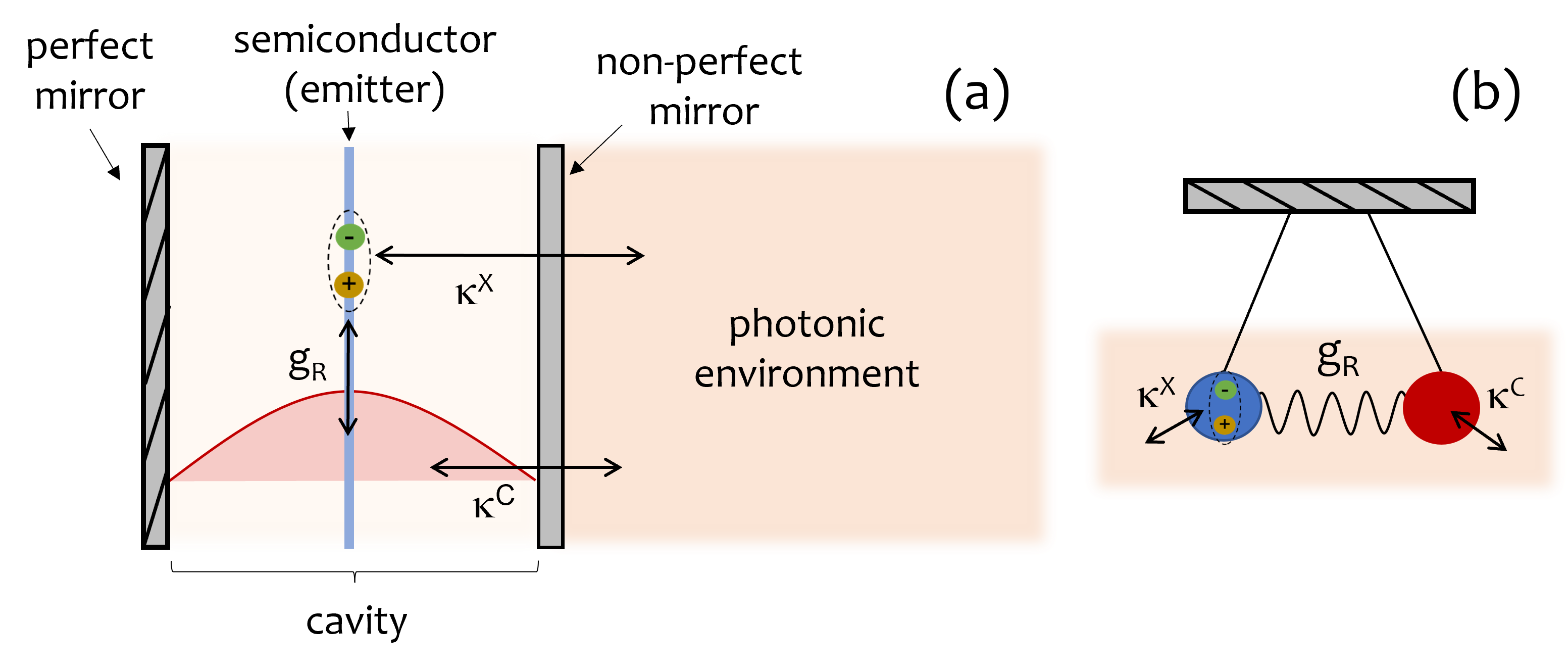
Figure 1: (a) Sketch of the hybrid light-matter system under consideration. It consists of a semiconductor layer embedded in a planar optical cavity. One of the mirrors is not perfect, which allows the emitter and the cavity photon to interact with the common photonic environment via the couplings $\kappa$. Panel (b) illustrates the analogy with two coupled oscillators immersed in a common medium.

The paper is organized as follows. The model and formalism are introduced in Section II. In Section III, we present the results obtained by making use of the memoryless approximation. Finally, in Section IV we extend the model to include non-radiative losses and calculate the reflection and absorption spectra. A brief summary and our conclusions are given in Section V. Additional information and technical details are provided in Appendices.

II Theoretical description

II.1 Model

We employ a system-environment decomposition, as is customary for the description of open quantum systems, and hence we start with a total Hamiltonian of the form $\hat{H}=\hat{H}_{S}+\hat{H}_{E}+\hat{H}_{SE}$. Here, $\hat{H}_{S}$ and $\hat{H}_{E}$ correspond to the system of interest and the environment, respectively, while $\hat{H}_{SE}$ describes the system-environment coupling. To be concrete, we consider the system illustrated in Fig. 1(a). It consists of two-dimensional excitons and cavity photons described by the Hamiltonian

$$\hat{H}_{S}=\sum_{\bf k}\left[\epsilon_{{\bf k}}^{C}\hat{c}_{{\bf k}}^{\dagger}\hat{c}_{{\bf k}}+\epsilon_{{\bf k}}^{X}\hat{x}_{{\bf k}}^{\dagger}\hat{x}_{{\bf k}}+g_{R}\left(\hat{x}_{{\bf k}}^{\dagger}\hat{c}_{{\bf k}}+\hat{c}_{{\bf k}}^{\dagger}\hat{x}_{{\bf k}}\right)\right].$$ (1)

Here, $\hat{c}_{\mathbf{k}}$ ($\hat{c}_{\mathbf{k}}^{\dagger}$) and $\hat{x}_{\mathbf{k}}$ ($\hat{x}_{\mathbf{k}}^{\dagger}$) are bosonic annihilation (creation) operators of cavity photons and quantum-well excitons, respectively, with in-plane momentum $\hbar\mathbf{k}$. The kinetic energies at low momenta are $\epsilon_{\mathbf{k}}^{C}=\epsilon_{0}+\hbar^{2}k^{2}/2m_{C}+\delta$ and $\epsilon_{\mathbf{k}}^{X}=\epsilon_{0}+\hbar^{2}k^{2}/2m_{X}$, where $k\equiv|{\bf k}|$ and $m_{C}$ ($m_{X}$) is the cavity photon (exciton) mass, while $\delta$ is the photon-exciton detuning and $\epsilon_{0}$ is the exciton transition energy. $g_{R}$ is the Rabi coupling, and we assume that the rotating wave approximation holds ($\epsilon_{0}\gg g_{R}$).

We consider the environment to be the electromagnetic field outside of the cavity. To describe this photonic bath, we use the following Hamiltonian

$$\hat{H}_{E}=\int dq\sum_{\mathbf{k}}\epsilon_{{\bf k},q}^{E}\hat{e}_{{\bf k}q}^{\dagger}\hat{e}_{{\bf k}q},$$ (2)

where $\hat{e}_{{\bf k}q}$ ($\hat{e}_{{\bf k}q}^{\dagger}$) are annihilation (creation) operators for photons outside the cavity with in- and out-of-plane wavevectors ${\bf k}$ and $q$, respectively, and $\epsilon_{{\bf k},q}^{E}=\hbar c\sqrt{k^{2}+q^{2}}$ is the corresponding photon kinetic energy.

Since we consider the situation where both the emitter and the cavity photons interact with the photonic environment, we describe the system-environment interaction with a Hamiltonian of the form $\hat{H}_{SE}=\hat{H}_{XE}+\hat{H}_{CE}$ with

$$\hat{H}_{XE} =\int dq\sum_{\mathbf{k}}\left(\kappa_{{\bf k},q}^{X}\hat{e}_{{\bf k}q}^{\dagger}\hat{x}_{{\bf k}}+h.c.\right),$$ (3a)

$$\hat{H}_{CE} =\int dq\sum_{\mathbf{k}}\left(\kappa_{{\bf k},q}^{C}\hat{e}_{{\bf k}q}^{\dagger}\hat{c}_{{\bf k}}+h.c.\right).$$ (3b)

$\hat{H}_{XE}$ encodes the fact that the probability of an exciton to recombine by emitting a photon directly to the environment is nonzero . In particular, this can become the dominant process for the radiative recombination of the emitter when the cavity mode and emitter frequencies are not resonant (i.e., the opposite of the Purcell effect Purcell (1946)). $\hat{H}_{CE}$ describes the cavity-environment coupling that exists even in the absence of the semiconductor layer. Crucially, the form of $\hat{H}_{SE}$ allows for interference effects to take place when the couplings $\kappa^{X}_{{\bf k},q}$ and $\kappa^{C}_{{\bf k},q}$ are both nonzero. This is an essential difference between the present model and those which consider independent environments for the emitter and the cavity (e.g., Refs. Carmichael et al. (1989); Cirac et al. (1991); Auffèves et al. (2008); Carmichael (2009); Andreani et al. (1999); Laucht et al. (2009); del Valle et al. (2009); Giesz et al. (2016); Verger et al. (2006); Laussy et al. (2008, 2009)). For each in-plane wavevector, the scenario we consider is analogous to the problem of two coupled oscillators immersed in a common medium illustrated in Fig. 1(b).

II.2 Input-output formalism

II.2.1 Time dependent equations

To obtain the time evolution of the system, we use an input-output approach Gardiner and Collett (1985); Ciuti and Carusotto (2006), which allows us to describe the response to an arbitrary input such as a coherent field. The key idea is to start from the Heisenberg equations of motion for the system and bath operators, and then eliminate the bath operators by using their initial conditions, i.e., the input, as detailed below.

The Heisenberg equations of motion for the system operators are

$$i\hbar\partial_{t}\hat{c}_{\bf k} = \left[\hat{c}_{\bf k},\hat{H}_{S}\right]+\int dq\,\kappa_{{\bf k},q}^{C*}\hat{e}_{{\bf k}q},$$ (4a)

$$i\hbar\partial_{t}\hat{x}_{\bf k} = \left[\hat{x}_{\bf k},\hat{H}_{S}\right]+\int dq\,\kappa_{{\bf k},q}^{X*}\hat{e}_{{\bf k}q}.$$ (4b)

In the same way, one obtains the evolution equations for the bath operators

$$i\hbar\partial_{t}\hat{e}_{{\bf k}q}= \epsilon_{{\bf k},q}^{E}\hat{e}_{{\bf k}q}+\kappa_{{\bf k},q}^{C}\hat{c}_{{\bf k}}+\kappa_{{\bf k},q}^{X}\hat{x}_{{\bf k}}.$$ (5)

The formal solution of Eq. (5) is of the form:

$$\hat{e}_{{\bf k}q}(t) =e^{-\frac{i}{\hbar}\epsilon_{{\bf k},q}^{E}(t-t_{0})}\hat{e}_{{\bf k}q}(t_{0})$$ (6)

$$+\frac{1}{i\hbar}\int_{t_{0}}^{t}dt^{\prime}e^{-\frac{i}{\hbar}\epsilon_{{\bf k},q}^{E}(t-t^{\prime})}\left(\kappa_{{\bf k},q}^{C}\hat{c}_{{\bf k}}(t^{\prime})+\kappa_{{\bf k},q}^{X}\hat{x}_{{\bf k}}(t^{\prime})\right).$$

If one defines input and output operators as

$$\hat{e}_{{\bf k}q}^{\text{I}} =\lim_{t_{0}\rightarrow-\infty}e^{\frac{i}{\hbar}\epsilon_{{\bf k},q}^{E}t_{0}}\hat{e}_{{\bf k}q}(t_{0}),$$ (7a)

$$\hat{e}_{{\bf k}q}^{\text{O}} =\lim_{t\rightarrow\infty}e^{\frac{i}{\hbar}\epsilon_{{\bf k},q}^{E}t}\hat{e}_{{\bf k}q}(t),$$ (7b)

one can use Eq. (6) to obtain the following relation

$$\hat{e}_{{\bf k}q}^{\text{O}}=\hat{e}_{{\bf k}q}^{\text{I}}+\frac{1}{i\hbar}\kappa_{{\bf k},q}^{C}\hat{\mathcal{C}}_{\bf k}(\omega_{{\bf k},q}^{E})+\frac{1}{i\hbar}\kappa_{{\bf k},q}^{X}\hat{\mathcal{X}}_{\bf k}(\omega_{{\bf k},q}^{E}).$$ (8)

Here, $\hat{\mathcal{A}}_{\bf k}(\omega)=\int dt\,e^{i\omega t}\hat{a}_{\bf k}(t)$ corresponds to the Fourier transform of the operator $\hat{a}_{\bf k}(t)$ and $\omega_{{\bf k},q}^{E}=\epsilon_{{\bf k},q}^{E}/\hbar$. We can see that Eq. (8) relates the output operator to those of the input and the system.

Inserting Eq. (6) into Eq. (4) and taking the limit $t_{0}\rightarrow-\infty$, one obtains the following equations for the system operators

$$i\hbar\partial_{t}\hat{c}_{\bf k} = \left[\hat{c}_{\bf k},\hat{H}_{S}\right]-i\int_{-\infty}^{\infty}dt^{\prime}\Gamma_{\bf k}^{CC}(t-t^{\prime})\hat{c}_{\bf k}(t^{\prime})-i\int_{-\infty}^{\infty}dt^{\prime}\Gamma_{\bf k}^{CX}(t-t^{\prime})\hat{x}_{\bf k}(t^{\prime})+\hat{F}_{\bf k}^{C}(t),$$ (9a)

$$i\hbar\partial_{t}\hat{x}_{\bf k} = \left[\hat{x}_{\bf k},\hat{H}_{S}\right]-i\int_{-\infty}^{\infty}dt^{\prime}\Gamma_{\bf k}^{XX}(t-t^{\prime})\hat{x}_{\bf k}(t^{\prime})-i\int_{-\infty}^{\infty}dt^{\prime}\Gamma_{\bf k}^{XC}(t-t^{\prime})\hat{c}_{\bf k}(t^{\prime})+\hat{F}_{\bf k}^{X}(t).$$ (9b)

Here, both the Langevin-like force operators $\hat{F}_{\bf k}^{X,C}(t)$ and the damping terms $\Gamma_{\bf k}^{AB}(\tau)$ originate from the interaction with the common photonic environment (3) and are not captured in $\hat{H}_{S}$. Importantly, we see that $\Gamma_{\bf k}^{CX}(\tau)$ in Eq. (9) induces an additional coupling between the excitons and cavity photons. Explicitly, one has

$$\Gamma_{\bf k}^{AB}(\tau) =\theta(\tau)\frac{1}{\hbar}\int dq\,\kappa_{{\bf k},q}^{A*}\kappa_{{\bf k},q}^{B}e^{-\frac{i}{\hbar}\epsilon_{{\bf k},q}^{E}\tau},$$ (10)

and the ‘force’ operators are related to the input operators as

$$\hat{F}_{\bf k}^{C}(t) = \int dq\,\kappa_{{\bf k},q}^{C*}e^{-\frac{i}{\hbar}\epsilon_{{\bf k},q}^{E}t}\hat{e}_{{\bf k}q}^{\text{I}},$$ (11a)

$$\hat{F}_{\bf k}^{X}(t) = \int dq\,\kappa_{{\bf k},q}^{X*}e^{-\frac{i}{\hbar}\epsilon_{{\bf k},q}^{E}t}\hat{e}_{{\bf k}q}^{\text{I}}.$$ (11b)

II.2.2 Frequency domain

Taking the Fourier transform of Eq. (9), we arrive at the matrix equation

$$\mathcal{M}({\bf k},\omega)\begin{pmatrix}\hat{\mathcal{C}}_{\bf k}(\omega)\\ \hat{\mathcal{X}}_{\bf k}(\omega)\end{pmatrix}=\begin{pmatrix}\hat{\mathcal{F}}_{{\bf k}}^{C}(\omega)\\ \hat{\mathcal{F}}_{{\bf k}}^{X}(\omega)\end{pmatrix}.$$ (12)

Here, $\hat{\mathcal{X}}_{\bf k}(\omega),\hat{\mathcal{C}}_{\bf k}(\omega),\hat{\mathcal{F}}_{\bf k}(\omega)$ denote the Fourier transforms of the operators $\hat{x}_{\bf k}(t),\hat{c}_{\bf k}(t),\hat{F}_{\bf k}(t)$ respectively, and

$$\mathcal{M}({\bf k},\omega)=\begin{pmatrix}\hbar\omega-\epsilon_{\bf k}^{C}+i\tilde{\Gamma}_{\bf k}^{CC}(\omega)&&-g_{R}+i\tilde{\Gamma}_{\bf k}^{CX}(\omega)\\ -g_{R}+i\tilde{\Gamma}_{\bf k}^{XC}(\omega)&&\hbar\omega-\epsilon_{\bf k}^{X}+i\tilde{\Gamma}_{\bf k}^{XX}(\omega)\end{pmatrix}.$$ (13)

We note that ${\cal M}^{-1}$ corresponds to the single-particle Green’s matrix of the system, modified by the interaction with the common photonic environment (see Appendix A). $\tilde{\Gamma}_{\bf k}^{AB}(\omega)$ denotes the Fourier transform of $\Gamma_{\bf k}^{AB}(\tau)$ and takes the form

$$\tilde{\Gamma}_{\bf k}^{AB}(\omega) =\frac{\pi}{\hbar}\int dq\,\kappa_{{\bf k},q}^{A*}\kappa_{{\bf k},q}^{B}\delta(\omega-\omega_{{\bf k},q}^{E})$$

$$\leavevmode\nobreak\ \leavevmode\nobreak\ \leavevmode\nobreak\ \leavevmode\nobreak\ \leavevmode\nobreak\ \leavevmode\nobreak\ +\frac{i}{\hbar}\mathcal{P}\int dq\frac{\kappa_{{\bf k},q}^{A*}\kappa_{{\bf k},q}^{B}}{\omega-\omega_{{\bf k},q}^{E}},$$ (14)

where $\mathcal{P}$ denotes the Cauchy principal value. The Fourier transform of the force operators are related to the input operator as

$$\hat{\mathcal{F}}_{{\bf k}}^{C}(\omega) =2\pi\kappa_{{\bf k},q_{p}}^{C*}\rho_{{\bf k}}(\omega)\hat{e}_{{\bf k},q_{p}}^{\text{I}},$$ (15a)

$$\hat{\mathcal{F}}_{{\bf k}}^{X}(\omega) =2\pi\kappa_{{\bf k},q_{p}}^{X*}\rho_{{\bf k}}(\omega)\hat{e}_{{\bf k},q_{p}}^{\text{I}},$$ (15b)

where the wavevector $q_{p}$ is defined by the resonance condition $\omega=\omega_{{\bf k},q_{p}}^{E}$ and we have introduced

$$\rho_{{\bf k}}(\omega)=(\partial_{q}\omega_{{\bf k},q}^{E})_{q=q_{p}}^{-1}.$$ (16)

Physically, $\rho_{{\bf k}}(\omega)$ corresponds to the photon environment density of states. It is real and well defined when $\omega>ck$, while when $\omega<ck$, it is not possible to emit radiation outside of the cavity since there are no free photon modes.

Inserting Eqs. (12) and (15) in Eq. (8), one obtains the following input-output relation

$$\hat{e}_{{\bf k},q_{p}}^{\text{O}}=S({\bf k},\omega)\hat{e}_{{\bf k},q_{p}}^{\text{I}},$$ (17)

where

$$S({\bf k},\omega)=1-i\frac{2\pi\rho_{{\bf k}}(\omega)}{\hbar}\sum_{i,j}\left[\mathcal{M}({\bf k},\omega)\right]_{ij}^{-1}\kappa_{{\bf k},q_{p}}^{i}\kappa_{{\bf k},q_{p}}^{j*}.$$ (18)

Here, $[\mathcal{M}({\bf k},\omega)]_{ij}^{-1}$ corresponds to the $(i,j)$th element of $\mathcal{M}^{-1}$. One can check that $|S({\bf k},\omega)|=1$, and therefore the transformation (17) is unitary. This implies that the output operators obey the same Bose commutation relations as the input operators. However, it is interesting to remark that the fact that we have a single common photonic bath with a given density of state $\rho_{{\bf k}}$ is important for this unitarity property. Indeed, in the different scenario where the emitter and cavity photon interact with independent matter and photon baths with different dispersion relations (i.e., different densities of states), the resulting input-output transformation cannot be unitary since it is not equivalent to have an input from the matter or from the photon bath. This subtlety seems to have been missed in Ref. Ciuti and Carusotto (2006), and must be accounted for to calculate reflection or absorption, as discussed in Sec. IV.

While these observables cannot be properly defined in a model with a single environment, one can use Eq. (12) to calculate the power spectrum

$$I({\bf k},\omega)=\langle\hat{\mathcal{C}}_{\bf k}^{\dagger}(\omega)\hat{\mathcal{C}}_{\bf k}(\omega)+\hat{\mathcal{X}}_{\bf k}^{\dagger}(\omega)\hat{\mathcal{X}}_{\bf k}(\omega)\rangle,$$ (19)

which encodes the emission spectrum of the system for a given input of the environment, such as a coherent drive. We note that in the absence of the environment, the right-hand side of Eq. (12) is zero and the power spectrum vanishes, as it should.

III Memoryless approximation and Non-Hermitian effects

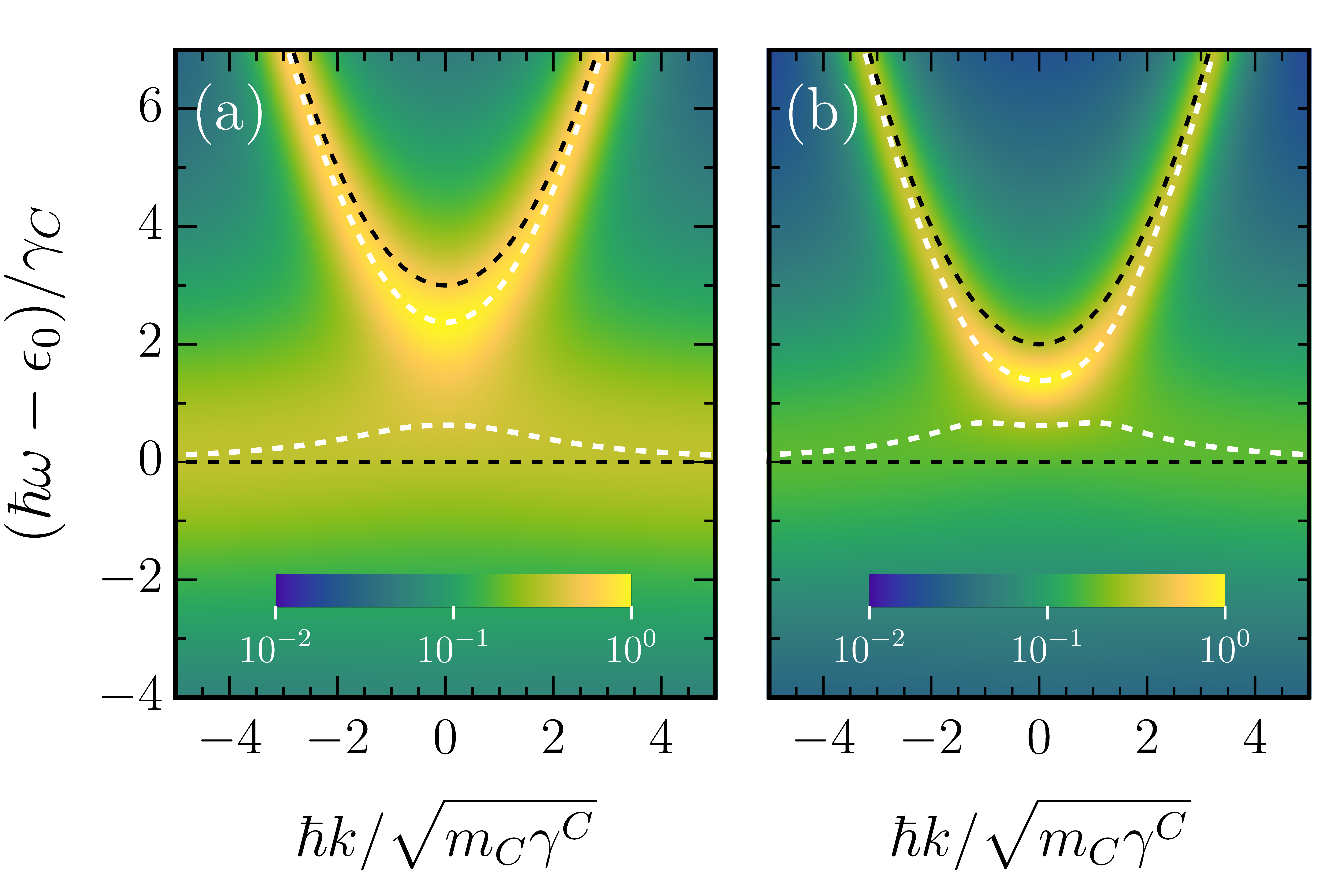
Figure 2: Anomalous dispersions. The color plots show the power spectra $I({\bf k},\omega)$ (color scale in arbitrary units). The dashed white lines correspond to the real parts of Eq. (22) and the dashed-black lines represent the bare exciton and cavity photon kinetic energies $\epsilon_{\bf k}^{X}$ and $\epsilon_{\bf k}^{C}$. (a) $\delta/\gamma^{C}=3$, (b) $\delta/\gamma^{C}=2$. The other parameters used for both panels are: $n_{\bf k}(\omega)=1$, $\gamma^{X}/\gamma^{C}=1.8$, $g_{R}/\gamma^{X}=0$, $m_{C}/m_{X}=0$.

The set of evolution equations in (9) implies that the system operators $\hat{c}_{\bf k},\hat{x}_{\bf k}$ at time $t$ are affected by their past at times $t^{\prime}<t$ through the functions $\Gamma_{\bf k}^{AB}(\tau)$. However, such memory effects disappear if we take the couplings $\kappa$ in Eq. (3) to be independent of $q$, and approximate $\Gamma_{\bf k}^{CC}(\tau)\simeq\gamma_{\bf k}^{C}\delta(\tau)$, $\Gamma_{\bf k}^{XX}(\tau)\simeq\gamma_{\bf k}^{X}\delta(\tau)$, and $\Gamma_{\bf k}^{CX}(\tau)\simeq\sqrt{\gamma_{\bf k}^{C}\gamma_{\bf k}^{X}}\delta(\tau)$, where $\gamma_{\bf k}^{C}$ and $\gamma_{\bf k}^{X}$ correspond to the photon and exciton linewidths, respectively. These can be related to the model parameters via (see Appendix B)

$$\gamma_{\bf k}^{C} =\pi\rho_{\bf k}(\omega_{0}^{X})|\kappa_{\bf k}^{C}|^{2}/\hbar,\leavevmode\nobreak\ \leavevmode\nobreak\ \gamma_{\bf k}^{X}=\pi\rho_{\bf k}(\omega_{0}^{X})|\kappa_{\bf k}^{X}|^{2}/\hbar.$$ (20)

where we have used $\rho_{{\bf k}}(\omega)\simeq\rho_{{\bf k}}(\omega_{0}^{X})$, with $\omega_{0}^{X}=\epsilon_{0}/\hbar$ , and we have assumed that $\arg(\kappa_{{\bf k}}^{C*}\kappa_{{\bf k}}^{X})=0$, since the two parts of the system (cavity-photon and exciton) are located at the same place. Such a memoryless approximation is also referred to as the Markov approximation Gardiner and Collett (1985), and we expect it to be accurate when $\epsilon_{\bf k}^{C},\epsilon_{\bf k}^{X}\gg\gamma_{\bf k}^{C},\gamma_{\bf k}^{X}$.

Within this approximation, the matrix (13) simplifies to

$$\mathcal{M}({\bf k},\omega)=\begin{pmatrix}\hbar\omega-z_{\bf k}^{C}&&-\tilde{g}_{\bf k}\\ -\tilde{g}_{\bf k}&&\hbar\omega-z_{\bf k}^{X}\end{pmatrix},$$ (21)

where we have introduced $z_{\bf k}^{C,X}=\epsilon_{\bf k}^{C,X}-i\gamma_{\bf k}^{C,X}$, and $\tilde{g}_{\bf k}=g_{R}-i\sqrt{\gamma_{\bf k}^{C}\gamma_{\bf k}^{X}}$. We can see that the matrix takes the form $\mathcal{M}({\bf k},\omega)=\hbar\omega\mathbb{1}-H_{{\bf k}}$, where $H_{{\bf k}}$ can be interpreted as an effective non-Hermitian Hamiltonian Ashida et al. (2020). Crucially, the imaginary part of the off-diagonal coupling is a consequence of the common environment, and would be absent in the typically assumed case of independent environments Ciuti and Carusotto (2006).

Solving $\det[\mathcal{M}]=0$, one obtains the complex eigenvalues

$$\hbar\omega_{\bf k}^{L,U} =\frac{1}{2}\left(z_{\bf k}^{C}+z_{\bf k}^{X}\pm\sqrt{(z_{\bf k}^{C}-z_{\bf k}^{X})^{2}+4\tilde{g}_{\bf k}^{2}}\right).$$ (22)

The power spectrum (19) can be calculated analytically and reads

$$I({\bf k},\omega) =\frac{A_{\bf k}(\omega)\gamma_{\bf k}^{C}+B_{\bf k}(\omega)\gamma_{\bf k}^{X}+D_{\bf k}(\omega)\sqrt{\gamma_{\bf k}^{X}\gamma_{\bf k}^{C}}}{|\hbar\omega-\hbar\omega_{\bf k}^{L}|^{2}|\hbar\omega-\hbar\omega_{\bf k}^{U}|^{2}}n_{\bf k}(\omega),$$ (23)

where $n_{\bf k}(\omega)=\pi\hbar\rho_{{\bf k}}(\omega_{0}^{X})\langle\hat{e}_{{\bf k},q_{p}}^{\text{I}\dagger}\hat{e}_{{\bf k},q_{p}}^{\text{I}}\rangle$ is proportional to the photon distribution in the input field and we have defined

$$A_{\bf k}(\omega) =4\left(|\tilde{g}_{\bf k}|^{2}+|\hbar\omega-z_{\bf k}^{X}|^{2}\right),$$

$$B_{\bf k}(\omega) =4\left(|\tilde{g}_{\bf k}|^{2}+|\hbar\omega-z_{\bf k}^{C}|^{2}\right),$$

$$D_{\bf k}(\omega) =8\real\left[(2\hbar\omega-z_{\bf k}^{C}-z_{\bf k}^{X})\tilde{g}_{\bf k}^{*}\right].$$

We emphasize that $\gamma_{\bf k}^{C}$ and $\gamma_{\bf k}^{X}$ only account for radiative decay into the common photonic environment. In realistic systems, there can also exist nonradiative photonic and excitonic losses. As we show in Section IV, these allow for absorption to take place and can be incorporated into Eqs. (21–23) by adding additional decay rates in the definition of $z_{\bf k}^{C},z_{\bf k}^{X}$. Importantly, the absorption spectrum can exhibit qualitatively similar features to the power spectrum. Here, we focus on the regime where such nonradiative losses are negligible with respect to $\gamma_{\bf k}^{X}$ and $\gamma_{\bf k}^{C}$. To shorten the notation in the discussion below, we introduce the $k$-dependent photon-exciton energy and linewidth detunings $\delta_{\epsilon_{\bf k}}=\real[z_{\bf k}^{C}-z_{\bf k}^{X}]$, and $\delta_{\gamma_{\bf k}}=-\imaginary[z_{\bf k}^{C}-z_{\bf k}^{X}]$.

III.1 Level attraction and anomalous dispersions

In the limit of negligible Rabi coupling, the argument of the square root in Eq. (22) can give rise to level attraction when $\delta_{\epsilon_{\bf k}}\neq 0$ and $\gamma_{\bf k}^{C}\sim\gamma_{\bf k}^{X}$. In particular, this effect provides a plausible and relatively simple explanation for recent puzzling photoluminescence measurements in semiconductor cavities Tawara et al. (2010); Dalacu et al. (2010); Valente et al. (2014); Dhara et al. (2018); Wurdack et al. (2023) which reported anomalous level attraction . In the opposite limit of strong Rabi coupling, $g_{R}\gg\gamma_{\bf k}^{C},\gamma_{\bf k}^{X},\delta_{\epsilon_{\bf k}}$, the argument of the square root in Eq. (22) gives rise to level repulsion and to the conventional lower and upper polariton modes Weisbuch et al. (1992). Finally, we note that when $\gamma_{\bf k}^{X}/\gamma_{\bf k}^{C}\rightarrow 0$, one recovers the case where the only radiative decay channel is from the cavity mode, as considered in Refs. Sachdev (1984); Barnett and Knight (1986); Agarwal and Puri (1986).

In order to illustrate the phenomenon of level attraction and to highlight how this can, in turn, lead to anomalous dispersion relations in planar cavities, we have plotted in Fig. 2 two examples of power spectra. For the purposes of this illustration, we have used decay parameters independent of the in-plane wavevector $\gamma^{C,X}$ and a vanishing Rabi coupling $g_{R}/\gamma^{C,X}\simeq 0$. The dispersion shown in panel (a) resembles the observation of Ref. Dhara et al. (2018), which reported an anomalous inverted parabolic behavior, i.e., a negative effective mass, of the lower line around $k=0$. While this effect was originally believed to have a many-body origin Dhara et al. (2018), it is not predicted by a recent more microscopic many-body theory Rana et al. (2021). The dispersion displayed in panel (b) resembles that reported in Ref. Wurdack et al. (2023), in which the inverted parabolic behavior of the lower line was observed at $k\neq 0$. We note that the power spectrum calculated here is not strictly equivalent to an experimental photoluminescence spectrum, as in such measurements some relaxation and partial thermalization take place which tends to favor the occupation of the lower energy states.

It is worth noticing that the single-mode version of the model in the regime $g_{R}/\gamma^{C,X}\simeq 0$ is potentially relevant for semiconductor quantum-dot cavities. As such, a dissipative coupling mediated by the common photon environment could also have played a role for the level attraction reported in photoluminescence measurements in these systems Tawara et al. (2010); Dalacu et al. (2010); Valente et al. (2014). In particular, we note that the observations of Ref. Tawara et al. (2010) could not be fully explained by their model, and that the paper evokes some ‘unknown mode-pulling effects’. We emphasize that the present mechanism is solely due to the common photonic environment, which was not considered in Tawara et al. (2010); Dalacu et al. (2010); Valente et al. (2014); Dhara et al. (2018); Wurdack et al. (2023), and it does not rely on material or temperature-dependent properties of solid-state emitters, nor on the pumping procedure.

III.2 Exceptional points and bound states in the continuum

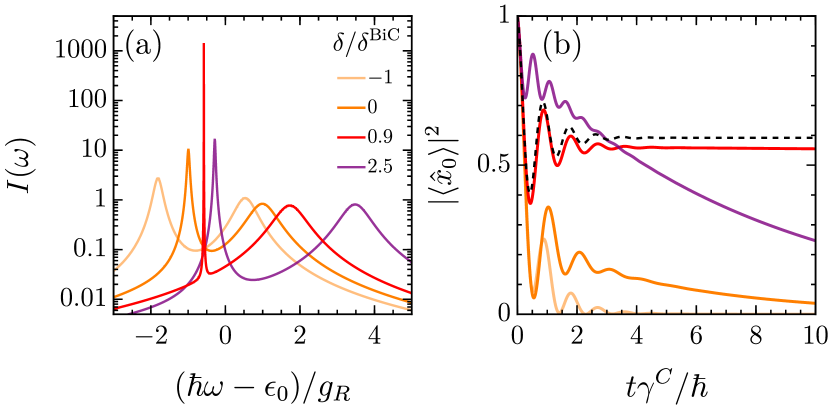
Figure 3: Vicinity of a bound state in the continuum. (a) Power spectra for different detunings. (b) Dynamics of $|\langle\hat{x}_{0}\rangle|^{2}$ with initial conditions $\langle\hat{x}_{0}(0)\rangle=1$, $\langle\hat{c}_{0}(0)\rangle=0$ and vacuum environment. The solid colored lines correspond to the same detunings used in panel (a) and the dashed black line corresponds to $\delta=\delta^{\text{BiC}}$ given in Eq. (25b). The other parameters used in both panels are $g_{R}/\gamma^{C}=3$, $\gamma^{X}/\gamma^{C}=0.3$, $k=0$.

Aside from the connection with recent experiments, the present model embeds additional interesting special cases. First, we note that exceptional points Berry (2004); Heiss (2012); Miri and Alù (2019) can arise when the square root in Eq. (22) vanishes . This occurs when the following conditions for the photon-exciton detunings are both satisfied:

$$\delta_{\epsilon_{\bf k}}^{\text{EP}} =\pm 2\sqrt{\gamma_{\bf k}^{C}\gamma_{\bf k}^{X}},\leavevmode\nobreak\ \leavevmode\nobreak\ \delta_{\gamma_{\bf k}}^{\text{EP}}=\mp 2g_{R}.$$ (24)

We note that these conditions would remain valid in the presence of an additional exciton broadening once it is incorporated into $\delta_{\gamma_{\bf k}}$; and that when $\gamma_{\bf k}^{X}=0$, Eq. (24) corresponds to the condition for the so-called weak to strong coupling crossover Savona et al. (1995); Andreani et al. (1999). EPs at such a crossover have been reported recently in Ref. Gao et al. (2018) which relied on a polarization dependent Rabi splitting. In our case, the Rabi coupling is constant and we have an in-plane isotropy such that Eq. (24) can give rise to rings of EPs which, to leading order in $m_{C}/m_{X}\ll 1$, occur at $\hbar k_{\text{EP}}=\sqrt{2m_{C}(\delta_{\epsilon_{\bf k}}^{\text{EP}}-\delta)}$ .

Another interesting configuration appears when $\delta_{\epsilon_{\bf k}}=\delta_{\epsilon_{\bf k}}^{\text{BiC}}\equiv g_{R}\delta_{\gamma_{\bf k}}/\sqrt{\gamma_{\bf k}^{C}\gamma_{\bf k}^{X}}$, in which case the imaginary part of $\omega_{\bf k}^{L}$ in Eq. (22) vanishes exactly. As a consequence, the corresponding modes remain undamped , which corresponds to the realization of bound states in the continuum Friedrich and Wintgen (1985); Hsu et al. (2016) (i.e., these states remain localized within the cavity despite the fact that they coexist with the continuum of photonic modes outside the cavity). These arise from the interference between two resonances (exciton and cavity photon) and are thus hybrid light-matter analogs of the BiCs proposed in Refs. Fonda and Newton (1960); Friedrich and Wintgen (1985). Like the EPs above, the condition $\delta_{\epsilon_{\bf k}}=\delta_{\epsilon_{\bf k}}^{\text{BiC}}$ in a planar cavity can give rise to a ring of BiCs occuring at $\hbar k_{\text{BiC}}=\sqrt{2m_{C}(\delta_{\epsilon_{\bf k}}^{\text{BiC}}-\delta)}$. To our knowledge, the possibility to achieve such a ring is a novelty of the present isotropic system with respect to previous BiC realisations in other platforms Hsu et al. (2016); Azzam and Kildishev (2021).

In Fig. 3(a), we have plotted the power spectrum at $k=0$ for different values of $\delta/\delta^{\text{BiC}}$. We can see that as the detuning approaches $\delta^{\text{BiC}}$ the width of the lower energy peak decreases and its amplitude increases. At exactly $\delta=\delta^{\text{BiC}}$, the width vanishes and the power spectrum (23) diverges as $(\omega-\omega_{0}^{L})^{-2}$ . To illustrate the impact of the BiC condition on the dynamics, in Fig. 3(b), we have plotted the amplitude of the exciton field as a function of time for the corresponding detunings. In this figure, we have used the solution of the memoryless equations of motion given in Appendix C with $\langle\hat{x}_{0}(t=0)\rangle=1$, and the environment and cavity mode in their vacuum state as initial conditions. We can observe damped oscillations at short times, while at long times, we see that the closer $\delta$ is to $\delta^{\text{BiC}}$, the lower is the decaying slope. At $\delta=\delta^{\text{BiC}}$, the time-dependent amplitudes can be expressed as

$$|\langle\hat{c}_{0}(t)\rangle|^{2} =\frac{1+e^{-\frac{2\gamma}{\hbar}t}-2e^{-\frac{\gamma}{\hbar}t}\cos[\frac{\tilde{\Omega}}{\hbar}t]}{\gamma^{2}}\gamma^{C}\gamma^{X},$$ (25a)

$$|\langle\hat{x}_{0}(t)\rangle|^{2} =\frac{\frac{\gamma^{C}}{\gamma^{X}}+\frac{\gamma^{X}}{\gamma^{C}}e^{-\frac{2\gamma}{\hbar}t}+2e^{-\frac{\gamma}{\hbar}t}\cos[\frac{\tilde{\Omega}}{\hbar}t]}{\gamma^{2}}\gamma^{C}\gamma^{X},$$ (25b)

with $\gamma=\gamma^{C}+\gamma^{X}$ and $\tilde{\Omega}=g_{R}\gamma/\sqrt{\gamma^{C}\gamma^{X}}$. We can clearly see that the amplitudes remain finite as $t\rightarrow\infty$ when $\gamma^{C},\gamma^{X}\neq 0$. In other words, the probabilities to find the emitter or the cavity excited do not vanish in the long time limit, which contrasts with the conventional behavior of damped vacuum Rabi oscillations in the absence of a common photonic environment.

IV Additional losses, Reflection and Absorption

In the presence of a single photonic environment, one cannot formally describe absorption or reflection. Indeed, in the absence of any other loss channels, all input photons eventually return into the same environment, and thus the reflection is necessarily unity. Therefore, to describe the absorption and reflection within the input-output formalism, one must include some additional losses in the model.

In realistic planar semiconductor cavities, there are several sources of nonradiative losses. For example, inhomogeneities of the mirrors can cause scattering of cavity photons into guided modes, while lattice phonons can cause scattering of excitons into nonradiative exciton states. We will model these by adding two independent baths with which the exciton and the cavity photon can interact

$$\hat{H}_{m} =\int dq\sum_{\mathbf{k}}\left[\epsilon_{{\bf k},q}^{m}\hat{m}_{{\bf k}q}^{\dagger}\hat{m}_{{\bf k}q}+\left(\kappa_{{\bf k},q}^{m}\hat{m}_{{\bf k}q}^{\dagger}\hat{x}_{{\bf k}}+h.c.\right)\right],$$ (26a)

$$\hat{H}_{\gamma} =\int dq\sum_{\mathbf{k}}\left[\epsilon_{{\bf k},q}^{\gamma}\hat{\gamma}_{{\bf k}q}^{\dagger}\hat{\gamma}_{{\bf k}q}+\left(\kappa_{{\bf k},q}^{\gamma}\hat{\gamma}_{{\bf k}q}^{\dagger}\hat{c}_{{\bf k}}+h.c.\right)\right].$$ (26b)

Here, $\epsilon_{{\bf k},q}^{m}$ and $\epsilon_{{\bf k},q}^{\gamma}$ correspond to the single particle energies in the distinct matter and photon baths respectively, and $\hat{m}_{{\bf k}q}$ and $\hat{\gamma}_{{\bf k}q}$ denote their annihilation operators.

The derivation provided in the Section II can be straightforwardly generalized to include these additional baths, and one obtains the modified matrix equation

$$\mathcal{M}^{\prime}({\bf k},\omega)\begin{pmatrix}\hat{\mathcal{C}}_{\bf k}(\omega)\\ \hat{\mathcal{X}}_{\bf k}(\omega)\end{pmatrix}=\begin{pmatrix}\hat{\mathcal{F}}_{{\bf k}}^{C}(\omega)+\hat{\mathcal{F}}_{{\bf k}}^{\gamma}(\omega)\\ \hat{\mathcal{F}}_{{\bf k}}^{X}(\omega)+\hat{\mathcal{F}}_{{\bf k}}^{m}(\omega)\end{pmatrix},$$ (27)

with

$$\mathcal{M}^{\prime}({\bf k},\omega)=\mathcal{M}({\bf k},\omega)+i\begin{pmatrix}\tilde{\Gamma}_{\bf k}^{\gamma}(\omega)&&0\\ 0&&\tilde{\Gamma}_{\bf k}^{m}(\omega)\end{pmatrix}.$$ (28)

We can see that Eq. (27) has a similar structure as Eq. (12), with the presence of the additional baths included in $\tilde{\Gamma}_{\bf k}^{m}(\omega)$, $\tilde{\Gamma}_{\bf k}^{\gamma}(\omega)$ and $\hat{\mathcal{F}}_{{\bf k}}^{m}(\omega)$, $\hat{\mathcal{F}}_{{\bf k}}^{\gamma}(\omega)$. In particular, we note that it gives rise to additional complex terms on the diagonal of the matrix $\mathcal{M}^{\prime}$ with respect to $\mathcal{M}$. Similarly to Eq. (II.2.2), these additional terms read

$$\tilde{\Gamma}_{\bf k}^{m}(\omega) =\frac{\pi}{\hbar}\int dq\,|\kappa_{{\bf k},q}^{m}|^{2}\delta(\omega-\omega_{{\bf k},q}^{m})+\frac{i}{\hbar}\mathcal{P}\int dq\frac{|\kappa_{{\bf k},q}^{m}|^{2}}{\omega-\omega_{{\bf k},q}^{m}},$$ (29a)

$$\tilde{\Gamma}_{\bf k}^{\gamma}(\omega) =\frac{\pi}{\hbar}\int dq\,|\kappa_{{\bf k},q}^{\gamma}|^{2}\delta(\omega-\omega_{{\bf k},q}^{\gamma})+\frac{i}{\hbar}\mathcal{P}\int dq\frac{|\kappa_{{\bf k},q}^{\gamma}|^{2}}{\omega-\omega_{{\bf k},q}^{\gamma}},$$ (29b)

with $\omega_{{\bf k},q}^{m}=\epsilon_{{\bf k},q}^{m}/\hbar$, and $\omega_{{\bf k},q}^{\gamma}=\epsilon_{{\bf k},q}^{\gamma}/\hbar$. In the same way as Eq. (15), the operators $\hat{\mathcal{F}}_{{\bf k}}^{m}(\omega)$, $\hat{\mathcal{F}}_{{\bf k}}^{\gamma}(\omega)$ are given by

$$\hat{\mathcal{F}}_{{\bf k}}^{m}(\omega) =2\pi\kappa_{{\bf k},q_{m}}^{m*}\rho_{{\bf k}}^{m}(\omega)\hat{m}_{{\bf k},q_{m}}^{\text{I}},$$ (30a)

$$\hat{\mathcal{F}}_{{\bf k}}^{\gamma}(\omega) =2\pi\kappa_{{\bf k},q_{\gamma}}^{\gamma*}\rho_{{\bf k}}^{\gamma}(\omega)\hat{\gamma}_{{\bf k},q_{\gamma}}^{\text{I}}.$$ (30b)

Here, however, $\rho_{{\bf k}}^{m}(\omega)$, $\rho_{{\bf k}}^{\gamma}(\omega)$ correspond to the density of states of the additional baths, and $\hat{m}_{{\bf k}q}^{\text{I}}$, $\hat{\gamma}_{{\bf k}q}^{\text{I}}$ denote their respective input operators, and $q_{m}$, $q_{\gamma}$ are defined by the resonance conditions $\omega=\omega^{m}_{{\bf k},q_{m}}$ and $\omega=\omega^{\gamma}_{{\bf k},q_{\gamma}}$.

IV.1 Generalized input-output relations

Due to the presence of the additional baths, the input-output relations are also modified. These can be expressed in a matrix form as

$$\begin{pmatrix}\hat{e}_{{\bf k},q_{p}}^{\text{O}}\\ \hat{m}_{{\bf k},q_{m}}^{\text{O}}\\ \hat{\gamma}_{{\bf k},q_{\gamma}}^{\text{O}}\end{pmatrix}=\mathcal{S}({\bf k},\omega)\begin{pmatrix}\hat{e}_{{\bf k},q_{p}}^{\text{I}}\\ \hat{m}_{{\bf k},q_{m}}^{\text{I}}\\ \hat{\gamma}_{{\bf k},q_{\gamma}}^{\text{I}}\end{pmatrix}.$$ (31)

$\mathcal{S}({\bf k},\omega)$ is a $3\times 3$ matrix, and its elements are

$$\mathcal{S}_{11}({\bf k},\omega) =1-i\frac{2\pi\rho_{{\bf k}}(\omega)}{\hbar}\bigg{(}\left[\mathcal{M}^{\prime}({\bf k},\omega)\right]_{11}^{-1}|\kappa_{{\bf k},q_{p}}^{C}|^{2}+\left[\mathcal{M}^{\prime}({\bf k},\omega)\right]_{22}^{-1}|\kappa_{{\bf k},q_{p}}^{X}|^{2}$$

$$\leavevmode\nobreak\ \leavevmode\nobreak\ \leavevmode\nobreak\ \leavevmode\nobreak\ \leavevmode\nobreak\ \leavevmode\nobreak\ \leavevmode\nobreak\ \leavevmode\nobreak\ \leavevmode\nobreak\ \leavevmode\nobreak\ \leavevmode\nobreak\ \leavevmode\nobreak\ \leavevmode\nobreak\ \leavevmode\nobreak\ \leavevmode\nobreak\ \leavevmode\nobreak\ \leavevmode\nobreak\ \leavevmode\nobreak\ \leavevmode\nobreak\ \leavevmode\nobreak\ \leavevmode\nobreak\ \leavevmode\nobreak\ \leavevmode\nobreak\ \leavevmode\nobreak\ +\left[\mathcal{M}^{\prime}({\bf k},\omega)\right]_{12}^{-1}\kappa_{{\bf k},q_{p}}^{C}\kappa_{{\bf k},q_{p}}^{X*}+\left[\mathcal{M}^{\prime}({\bf k},\omega)\right]_{21}^{-1}\kappa_{{\bf k},q_{p}}^{X}\kappa_{{\bf k},q_{p}}^{C*}\bigg{)},$$ (32a)

$$\mathcal{S}_{22}({\bf k},\omega) =1-i\frac{2\pi\rho_{{\bf k}}^{m}(\omega)}{\hbar}\left[\mathcal{M}^{\prime}({\bf k},\omega)\right]_{22}^{-1}|\kappa_{{\bf k},q_{m}}^{m}|^{2},$$ (32b)

$$\mathcal{S}_{33}({\bf k},\omega) =1-i\frac{2\pi\rho_{{\bf k}}^{\gamma}(\omega)}{\hbar}\left[\mathcal{M}^{\prime}({\bf k},\omega)\right]_{11}^{-1}|\kappa_{{\bf k},q_{\gamma}}^{\gamma}|^{2},$$ (32c)

$$\mathcal{S}_{12}({\bf k},\omega) =-i\frac{2\pi\rho_{{\bf k}}^{m}(\omega)}{\hbar}\left(\left[\mathcal{M}^{\prime}({\bf k},\omega)\right]_{12}^{-1}\kappa_{{\bf k},q_{p}}^{C}\kappa_{{\bf k},q_{m}}^{m*}+\left[\mathcal{M}^{\prime}({\bf k},\omega)\right]_{22}^{-1}\kappa_{{\bf k},q_{p}}^{X}\kappa_{{\bf k},q_{m}}^{m*}\right),$$ (32d)

$$\mathcal{S}_{13}({\bf k},\omega) =-i\frac{2\pi\rho_{{\bf k}}^{\gamma}(\omega)}{\hbar}\left(\left[\mathcal{M}^{\prime}({\bf k},\omega)\right]_{11}^{-1}\kappa_{{\bf k},q_{p}}^{C}\kappa_{{\bf k},q_{\gamma}}^{\gamma*}+\left[\mathcal{M}^{\prime}({\bf k},\omega)\right]_{21}^{-1}\kappa_{{\bf k},q_{p}}^{X}\kappa_{{\bf k},q_{\gamma}}^{\gamma*}\right),$$ (32e)

$$\mathcal{S}_{21}({\bf k},\omega) =-i\frac{2\pi\rho_{{\bf k}}(\omega)}{\hbar}\left(\left[\mathcal{M}^{\prime}({\bf k},\omega)\right]_{21}^{-1}\kappa_{{\bf k},q_{p}}^{C*}\kappa_{{\bf k},q_{m}}^{m}+\left[\mathcal{M}^{\prime}({\bf k},\omega)\right]_{22}^{-1}\kappa_{{\bf k},q_{p}}^{X*}\kappa_{{\bf k},q_{m}}^{m}\right),$$ (32f)

$$\mathcal{S}_{31}({\bf k},\omega) =-i\frac{2\pi\rho_{{\bf k}}(\omega)}{\hbar}\left(\left[\mathcal{M}^{\prime}({\bf k},\omega)\right]_{11}^{-1}\kappa_{{\bf k},q_{p}}^{C*}\kappa_{{\bf k},q_{\gamma}}^{\gamma}+\left[\mathcal{M}^{\prime}({\bf k},\omega)\right]_{12}^{-1}\kappa_{{\bf k},q_{p}}^{X*}\kappa_{{\bf k},q_{\gamma}}^{\gamma}\right)$$ (32g)

$$\mathcal{S}_{23}({\bf k},\omega) =-i\frac{2\pi\rho_{{\bf k}}^{\gamma}(\omega)}{\hbar}\left[\mathcal{M}^{\prime}({\bf k},\omega)\right]_{21}^{-1}\kappa_{{\bf k},q_{p}}^{\gamma*}\kappa_{{\bf k},q_{m}}^{m},$$ (32h)

$$\mathcal{S}_{32}({\bf k},\omega) =-i\frac{2\pi\rho_{{\bf k}}^{m}(\omega)}{\hbar}\left[\mathcal{M}^{\prime}({\bf k},\omega)\right]_{12}^{-1}\kappa_{{\bf k},q_{m}}^{m*}\kappa_{{\bf k},q_{\gamma}}^{\gamma}.$$ (32i)

We note that in the absence of the common environment (i.e., when $\kappa_{{\bf k},q}^{X}=0$ and $\kappa_{{\bf k},q}^{C}=0$), one recovers the input-output relation obtained in Ref. Ciuti and Carusotto (2006) in the case of two independent baths for the cavity photons and the excitons. However, as we mentioned above, the transformation $\mathcal{S}$ cannot be unitary when the different baths are not equivalent.

IV.2 Reflection and Absorption

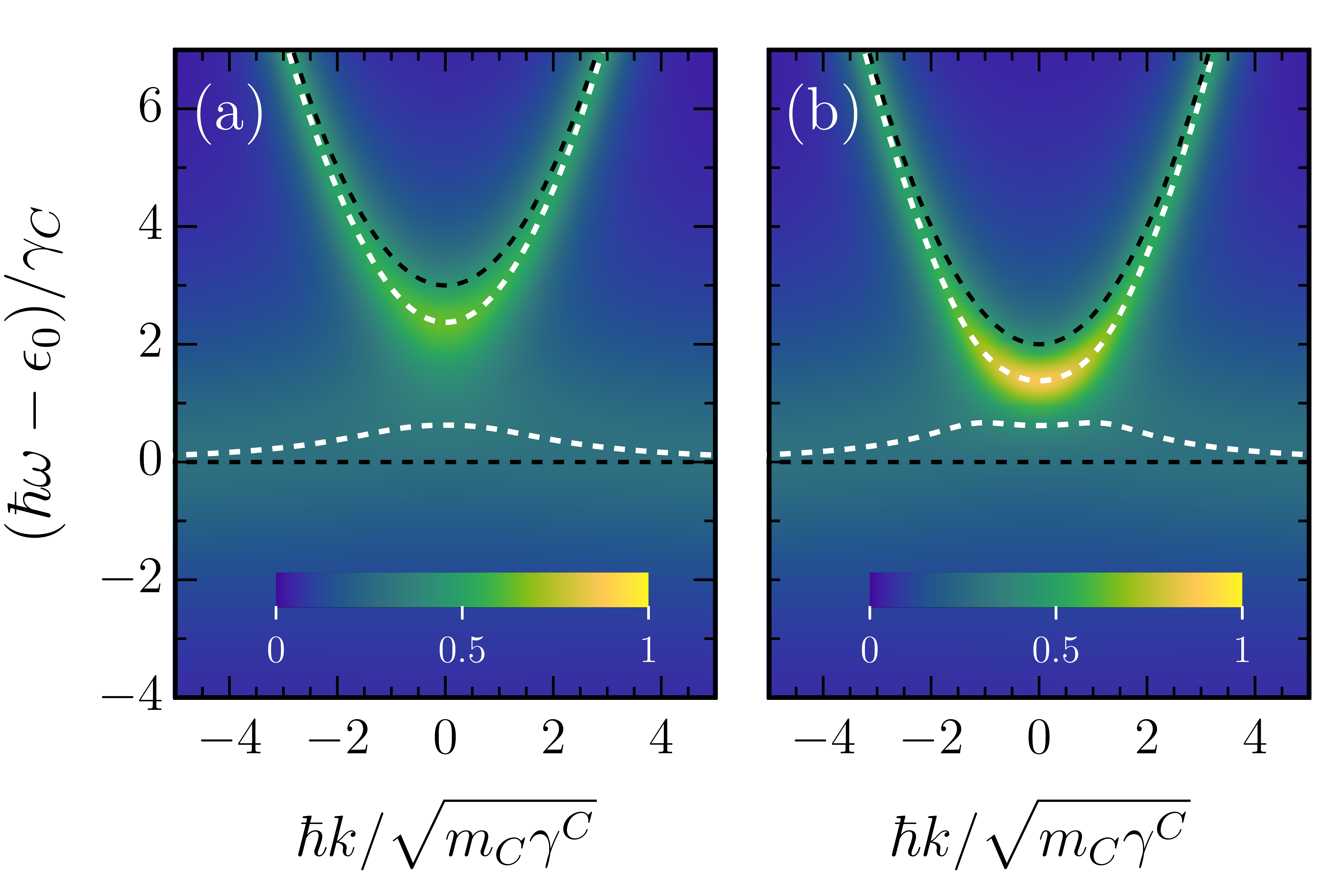
Figure 4: Absorption spectra. The color plots are obtained from Eq. (35). The dashed white lines correspond to the real parts of the eigenvalues [Eq. (22)] and the dashed-black lines represent the bare exciton and cavity photon kinetic energies $\epsilon_{\bf k}^{X}$ and $\epsilon_{\bf k}^{C}$. In both panels, the nonradiative decay parameters are $\gamma^{\gamma}/\gamma^{C}=\gamma^{m}/\gamma^{C}=0.15$. All the others parameters are identical to the ones used in Figure 2.

In order to introduce the notions of reflection and absorption one needs to use the conservation of the total particle number in the baths. This is given by the relation

$$\int d\omega\left[\rho_{\bf k}(\omega)\langle\hat{e}_{{\bf k},q_{p}}^{\text{O}\dagger}\hat{e}_{{\bf k},q_{p}}^{\text{O}}\rangle+\rho_{\bf k}^{m}(\omega)\langle\hat{m}_{{\bf k},q_{m}}^{\text{O}\dagger}\hat{m}_{{\bf k},q_{m}}^{\text{O}}\rangle+\rho_{\bf k}^{\gamma}(\omega)\langle\hat{\gamma}_{{\bf k},q_{\gamma}}^{\text{O}\dagger}\hat{\gamma}_{{\bf k},q_{\gamma}}^{\text{O}}\rangle\right]$$

$$\leavevmode\nobreak\ \leavevmode\nobreak\ \leavevmode\nobreak\ =\int d\omega\left[\rho_{\bf k}(\omega)\langle\hat{e}_{{\bf k},q_{p}}^{\text{I}\dagger}\hat{e}_{{\bf k},q_{p}}^{\text{I}}\rangle+\rho_{\bf k}^{m}(\omega)\langle\hat{m}_{{\bf k},q_{m}}^{\text{I}\dagger}\hat{m}_{{\bf k},q_{m}}^{\text{I}}\rangle+\rho_{\bf k}^{\gamma}(\omega)\langle\hat{\gamma}_{{\bf k},q_{\gamma}}^{\text{I}\dagger}\hat{\gamma}_{{\bf k},q_{\gamma}}^{\text{I}}\rangle\right].$$ (33)

The fact that the three baths are different is accounted for by the density of states.

In a reflection/absorption experiment, one excites the system from the photonic environment outside of the cavity while the other baths are initially in their vacuum states; hence, one has $\langle\hat{e}_{{\bf k},q_{p}}^{\text{I}\dagger}\hat{e}_{{\bf k},q_{p}}^{\text{I}}\rangle\neq 0$ and the other input averages are zero. One can then use Eq. (31) to express the output averages in term of the input ones such that Eq. (IV.2) reduces to

$$\rho_{\bf k}(1-|\mathcal{S}_{11}({\bf k},\omega)|^{2})-|\mathcal{S}_{21}({\bf k},\omega)|^{2}\rho_{\bf k}^{m}-|\mathcal{S}_{31}({\bf k},\omega)|^{2}\rho_{\bf k}^{\gamma}=0,$$

from which we can deduce the reflection and absorption spectra

$$\mathcal{R}({\bf k},\omega) =|\mathcal{S}_{11}({\bf k},\omega)|^{2},$$ (34a)

$$\mathcal{A}({\bf k},\omega) =|\mathcal{S}_{21}({\bf k},\omega)|^{2}\frac{\rho_{\bf k}^{m}}{\rho_{\bf k}}+|\mathcal{S}_{31}({\bf k},\omega)|^{2}\frac{\rho_{\bf k}^{\gamma}}{\rho_{\bf k}}.$$ (34b)

We note that the relation $\mathcal{R}+\mathcal{A}=1$ is respected, as it should, in the absence of any transmission. (We recall that no transmission can occur in the scenario we consider since only one mirror is not perfect, as schematized in Figure 1(a)).

Within the memoryless approximation, the absorption spectrum can be expressed as

$$\mathcal{A}({\bf k},\omega)=\gamma_{\bf k}^{\gamma}A_{\gamma}({\bf k},\omega)+\gamma_{\bf k}^{m}A_{m}({\bf k},\omega),$$ (35)

with

$$A_{\gamma}({\bf k},\omega) =4\frac{\gamma_{\bf k}^{C}|\hbar\omega-z_{\bf k}^{X}|^{2}+\gamma_{\bf k}^{X}|\tilde{g}_{\bf k}|^{2}}{|\hbar\omega-z_{\bf k}^{L}|^{2}|\hbar\omega-z_{\bf k}^{U}|^{2}}$$ (36a)

$$\leavevmode\nobreak\ \leavevmode\nobreak\ \leavevmode\nobreak\ +8\sqrt{\gamma_{\bf k}^{X}\gamma_{\bf k}^{C}}\frac{\real\left[\tilde{g}_{\bf k}^{*}(\hbar\omega-z_{\bf k}^{X})\right]}{|\hbar\omega-z_{\bf k}^{L}|^{2}|\hbar\omega-z_{\bf k}^{U}|^{2}},$$

$$A_{m}({\bf k},\omega) =4\frac{\gamma_{\bf k}^{C}|\tilde{g}_{\bf k}|^{2}+\gamma_{\bf k}^{X}|\hbar\omega-z_{\bf k}^{C}|^{2}}{|\hbar\omega-z_{\bf k}^{L}|^{2}|\hbar\omega-z_{\bf k}^{U}|^{2}}$$ (36b)

$$\leavevmode\nobreak\ \leavevmode\nobreak\ \leavevmode\nobreak\ +8\sqrt{\gamma_{\bf k}^{X}\gamma_{\bf k}^{C}}\frac{\real\left[\tilde{g}_{\bf k}^{*}(\hbar\omega-z_{\bf k}^{C})\right]}{|\hbar\omega-z_{\bf k}^{L}|^{2}|\hbar\omega-z_{\bf k}^{U}|^{2}}.$$

Here, we have $z_{\bf k}^{X}=\epsilon_{\bf k}^{X}-i\gamma_{\bf k}^{X}-i\gamma_{\bf k}^{m}$ and $z_{\bf k}^{C}=\epsilon_{\bf k}^{C}-i\gamma_{\bf k}^{C}-i\gamma_{\bf k}^{\gamma}$, and the additional photon and matter decay parameters $\gamma_{\bf k}^{\gamma},\gamma_{\bf k}^{m}$ are defined in a similar way as $\gamma_{\bf k}^{X}$ and $\gamma_{\bf k}^{C}$ with

$$\gamma_{\bf k}^{m} =\pi\rho_{\bf k}^{m}(\omega_{0}^{X})|\kappa_{\bf k}^{m}|^{2}/\hbar,\leavevmode\nobreak\ \leavevmode\nobreak\ \gamma_{\bf k}^{\gamma}=\pi\rho_{\bf k}^{\gamma}(\omega_{0}^{X})|\kappa_{\bf k}^{\gamma}|^{2}/\hbar.$$ (37)

Since in an absorption experiment the input is from the common photonic environment, the analytical expression we obtained previously for the power spectrum (23) remains valid once the additional decays are included in $z_{\bf k}^{X}$ and $z_{\bf k}^{C}$. One can then observe that the power spectrum is related to the absorption spectrum as

$$I({\bf k},\omega)=\left(A_{\gamma}({\bf k},\omega)+A_{m}({\bf k},\omega)\right)n_{\bf k}(\omega).$$ (38)

Interestingly, we can see that the contributions from $A_{\gamma}({\bf k},\omega)$ and $A_{m}({\bf k},\omega)$ are weighted by the nonradiative loss strengths in the absorption spectrum (35) but not in the power spectrum. This difference is related to the fact that there are two independent channels for absorption to take place, while the power spectrum can be defined in the absence of these nonradiative channels.

In Figure 4, we have plotted the absorption spectra using the parameters used in Figure 2 and symmetric nonradiative decay parameters $\gamma^{\gamma}/\gamma^{C}=\gamma^{m}/\gamma^{C}=0.15$. Apart from the different color scale, we can see that the absorption spectrum exhibits similar features as the power spectrum, as expected. This demonstrates that, in principle, one can experimentally access the anomalous dispersions in absorption measurements.

V Conclusions

We have demonstrated that the presence of a common photonic environment can lead to an effective dissipative coupling between light and matter in a nonideal cavity. Using a memoryless approximation, we have obtained analytical results for the power spectrum and the complex eigenenergies of this open system. This allowed us to highlight a potential connection with recent experiments that have reported anomalous level attraction, and to provide simple conditions under which rings of EPs and BiCs are expected. Furthermore, we have extended the model to incorporate non-radiative losses, thereby demonstrating that level attraction and anomalous dispersions could be probed in absorption experiments.

Our results open up intriguing perspectives. The inclusion of nonlinearities, which are system-dependent, could unveil novel regimes to generate photon antibunching in cavity systems Imamoḡlu et al. (1997); Verger et al. (2006); Liew and Savona (2010); Bamba et al. (2011); Gullans et al. (2013). Furthermore, to our knowledge, the possibility for the emitters and the cavity modes to interact with a common photonic environment is not accounted for in the usual models for single photon sources Auffèves et al. (2009); Grange et al. (2015); Choi et al. (2019) or laser theories Haken (1985), and it could be interesting to investigate whether it affects some of their properties. In this context, one expects that the hybrid light-matter BiC condition could favor low threshold lasing as evidenced with photonic BiCs Hsu et al. (2016); Azzam and Kildishev (2021); Kodigala et al. (2017).

Appendix A Connection to the Green’s function formalism

In this Appendix, we highlight the connection between the matrix $\mathcal{M}$ derived in the main text and the Green’s matrix of the system in presence of a common environment. The system single particle retarded Green’s matrix can be defined as

$$\mathbb{G}({\bf k},t)=\begin{pmatrix}G_{CC}({\bf k},t)&&G_{CX}({\bf k},t)\\ G_{XC}({\bf k},t)&&G_{XX}({\bf k},t)\end{pmatrix}=-\frac{i}{\hbar}\theta(t)\begin{pmatrix}\langle\hat{c}_{\bf k}(t)\hat{c}_{\bf k}^{\dagger}(0)\rangle&&\langle\hat{c}_{\bf k}(t)\hat{x}_{\bf k}^{\dagger}(0)\rangle\\ \langle\hat{x}_{\bf k}(t)\hat{c}_{\bf k}^{\dagger}(0)\rangle&&\langle\hat{x}_{\bf k}(t)\hat{x}_{\bf k}^{\dagger}(0)\rangle\end{pmatrix},$$ (39)

where the averages are taken over the vacuum. The cavity photon and exciton Green’s functions correspond to the diagonal elements of this matrix. It is also convenient to introduce the following system-environment retarded Green’s functions

$$G_{eC}({\bf k},q,t) =-\frac{i}{\hbar}\theta(t)\langle\hat{e}_{{\bf k}q}(t)\hat{c}_{\bf k}^{\dagger}(0)\rangle,$$ (40a)

$$G_{eX}({\bf k},q,t) =-\frac{i}{\hbar}\theta(t)\langle\hat{e}_{{\bf k}q}(t)\hat{x}_{\bf k}^{\dagger}(0)\rangle.$$ (40b)

Taking the time derivative of Eq. (39) gives

$$i\hbar\partial_{t}\mathbb{G}({\bf k},t) =\delta(t)\begin{pmatrix}\langle\hat{c}_{\bf k}(t)\hat{c}_{\bf k}^{\dagger}(0)\rangle&&\langle\hat{c}_{\bf k}(t)\hat{x}_{\bf k}^{\dagger}(0)\rangle\\ \langle\hat{x}_{\bf k}(t)\hat{c}_{\bf k}^{\dagger}(0)\rangle&&\langle\hat{x}_{\bf k}(t)\hat{x}_{\bf k}^{\dagger}(0)\rangle\end{pmatrix}-\frac{i}{\hbar}\theta(t)\begin{pmatrix}\langle i\hbar\partial_{t}\hat{c}_{\bf k}(t)\hat{c}_{\bf k}^{\dagger}(0)\rangle&&\langle i\hbar\partial_{t}\hat{c}_{\bf k}(t)\hat{x}_{\bf k}^{\dagger}(0)\rangle\\ \langle i\hbar\partial_{t}\hat{x}_{\bf k}(t)\hat{c}_{\bf k}^{\dagger}(0)\rangle&&\langle i\hbar\partial_{t}\hat{x}_{\bf k}(t)\hat{x}_{\bf k}^{\dagger}(0)\rangle\end{pmatrix}.$$ (41)

One can then use the equations of motion for the system operators to re-express the second term on the right hand side. Since the total Hamiltonian considered here only contains single-body couplings, the elements of this term can be expressed as linear combinations of single particle Green’s functions.

Making use of the equations of motion for the system operators (4), and Fourier transformation, one can obtain

$$\hbar\omega\mathcal{G}_{CC}({\bf k},\omega) =\epsilon_{\bf k}^{C}\mathcal{G}_{CC}({\bf k},\omega)+g_{R}\mathcal{G}_{XC}({\bf k},\omega)+\int dq\,\kappa_{{\bf k},q}^{C*}\mathcal{G}_{eC}({\bf k},q,\omega)+1,$$ (42a)

$$\hbar\omega\mathcal{G}_{XX}({\bf k},\omega) =\epsilon_{\bf k}^{X}\mathcal{G}_{XX}({\bf k},\omega)+g_{R}\mathcal{G}_{CX}({\bf k},\omega)+\int dq\,\kappa_{{\bf k},q}^{X*}\mathcal{G}_{eX}({\bf k},q,\omega)+1,$$ (42b)

$$\hbar\omega\mathcal{G}_{XC}({\bf k},\omega) =\epsilon_{\bf k}^{X}\mathcal{G}_{XC}({\bf k},\omega)+g_{R}\mathcal{G}_{CC}({\bf k},\omega)+\int dq\,\kappa_{{\bf k},q}^{X*}\mathcal{G}_{eC}({\bf k},q,\omega),$$ (42c)

$$\hbar\omega\mathcal{G}_{CX}({\bf k},\omega) =\epsilon_{\bf k}^{C}\mathcal{G}_{CX}({\bf k},\omega)+g_{R}\mathcal{G}_{XX}({\bf k},\omega)+\int dq\,\kappa_{{\bf k},q}^{C*}\mathcal{G}_{eX}({\bf k},q,\omega),$$ (42d)

where $\mathcal{G}_{AB}$ denotes the Fourier transform of $G_{AB}$. The same procedure applied to the system-environment Green’s functions (40) gives

$$\hbar\omega\mathcal{G}_{eC}({\bf k},q,\omega) =\epsilon_{{\bf k},q}^{E}\mathcal{G}_{eC}({\bf k},q,\omega)+\kappa_{{\bf k},q}^{C}\mathcal{G}_{CC}({\bf k},\omega)+\kappa_{{\bf k},q}^{X}\mathcal{G}_{XC}({\bf k},\omega),$$ (43a)

$$\hbar\omega\mathcal{G}_{eX}({\bf k},q,\omega) =\epsilon_{{\bf k},q}^{E}\mathcal{G}_{eX}({\bf k},q,\omega)+\kappa_{{\bf k},q}^{C}\mathcal{G}_{CX}({\bf k},\omega)+\kappa_{{\bf k},q}^{X}\mathcal{G}_{XX}({\bf k},\omega).$$ (43b)

We can now inject the system-environment Green’s function obtained from Eq. (43) into Eq. (42) and obtain the matrix equation

$$\begin{pmatrix}\hbar\omega-\epsilon_{\bf k}^{C}+i\tilde{\Gamma}_{\bf k}^{CC}(\omega)&&-g_{R}+i\tilde{\Gamma}_{\bf k}^{CX}(\omega)\\ -g_{R}+i\tilde{\Gamma}_{\bf k}^{XC}(\omega)&&\hbar\omega-\epsilon_{\bf k}^{X}+i\tilde{\Gamma}_{\bf k}^{XX}(\omega)\end{pmatrix}\begin{pmatrix}\mathcal{G}_{CC}({\bf k},\omega)&&\mathcal{G}_{CX}({\bf k},\omega)\\ \mathcal{G}_{XC}({\bf k},\omega)&&\mathcal{G}_{XX}({\bf k},\omega)\end{pmatrix}=\mathbb{1},$$ (44)

where $\mathbb{1}$ is the identity matrix. In Eq. (44), one can recognize the matrix $\mathcal{M}({\bf k},\omega)$ given in Eq. (13) of the main text, and observe that it corresponds to the inverse of the system retarded Green’s matrix in frequency space.

Appendix B Memoryless approximation

The set of evolution equations in (9) shows that the system operators $\hat{c}_{\bf k},\hat{x}_{\bf k}$ at time $t$ are affected by all their past at times $t^{\prime}<t$. This influence is encoded in the functions $\Gamma_{\bf k}^{AB}(\tau)$ defined in Eq. (10). As mentioned in the main text, one can simplify these equations by using a memoryless approximation. One can motivate this approximation by inspecting the functions $\Gamma_{\bf k}^{AB}(\tau)$

$$\Gamma_{\bf k}^{AB}(\tau) = \theta(\tau)\frac{1}{\hbar}\int_{-\infty}^{\infty}dq\,\kappa_{{\bf k},q}^{A*}\kappa_{{\bf k},q}^{B}e^{-\frac{i}{\hbar}\epsilon_{{\bf k},q}^{E}\tau}$$ (45)

$$= \theta(\tau)\frac{1}{\hbar}\int_{0}^{\infty}d\omega\,\rho_{{\bf k}}(\omega)\kappa_{{\bf k},q_{p}}^{A*}\kappa_{{\bf k},q_{p}}^{B}e^{-i\omega\tau}.$$ (46)

We expect the system-environment coupling strengths to be non-negligible only when the environment frequencies are in the vicinity of the system ones. Since the relevant frequencies are large (these are in the vicinity of the emitter frequency $\omega_{0}^{X}=\epsilon_{0}/\hbar$), we can neglect the frequency dependence of $\kappa_{{\bf k},q_{p}}^{A}\simeq\kappa_{{\bf k}}^{A}$ and take $\rho_{{\bf k}}(\omega)\simeq\rho_{{\bf k}}(\omega_{0}^{X})$. Then one has

$$\int_{0}^{\infty}d\omega\,\rho_{{\bf k}}(\omega)\kappa_{{\bf k},q_{p}}^{A*}\kappa_{{\bf k},q_{p}}^{B}e^{-i\omega\tau}$$

$$\leavevmode\nobreak\ \leavevmode\nobreak\ \simeq e^{-i\omega_{0}^{X}\tau}\int_{-\infty}^{\infty}d\omega\,\rho_{{\bf k}}(\omega_{0}^{X})\kappa_{{\bf k}}^{A*}\kappa_{{\bf k}}^{B}e^{-i\omega\tau}$$ (47)

$$\leavevmode\nobreak\ \leavevmode\nobreak\ =2\pi\rho_{{\bf k}}(\omega_{0}^{X})\kappa_{{\bf k}}^{A*}\kappa_{{\bf k}}^{B}\delta(\tau),$$ (48)

and thus one can approximate

$$\Gamma_{\bf k}^{AB}(\tau)\simeq\frac{\pi}{\hbar}\rho_{\bf k}(\omega_{0}^{X})\kappa_{\bf k}^{A*}\kappa_{\bf k}^{B}\delta(\tau).$$ (49)

Assuming $\arg(\kappa_{{\bf k}}^{C*}\kappa_{{\bf k}}^{X})=0$, in this approximation, Eqs. (9) reduce to

$$i\hbar\partial_{t}\hat{c}_{\bf k} =z_{\bf k}^{C}\hat{c}_{\bf k}+\tilde{g}_{\bf k}\hat{x}_{\bf k}+\hat{F}_{\bf k}^{C},$$ (50a)

$$i\hbar\partial_{t}\hat{x}_{\bf k} =z_{\bf k}^{X}\hat{x}_{\bf k}+\tilde{g}_{\bf k}\hat{c}_{\bf k}+\hat{F}_{\bf k}^{X},$$ (50b)

with $z_{\bf k}^{C,X}=\epsilon_{\bf k}^{C,X}-i\gamma_{\bf k}^{C,X}$ and $\tilde{g}_{\bf k}=g_{R}-i\sqrt{\gamma_{\bf k}^{C}\gamma_{\bf k}^{X}}$ and the decay parameters

$$\gamma_{\bf k}^{C} =\pi\rho_{\bf k}(\omega_{0}^{X})|\kappa_{\bf k}^{C}|^{2}/\hbar,\leavevmode\nobreak\ \leavevmode\nobreak\ \gamma_{\bf k}^{X}=\pi\rho_{\bf k}(\omega_{0}^{X})|\kappa_{\bf k}^{X}|^{2}/\hbar.$$ (51)

This leads to a simplification of the matrix (13) into (21) in the main text. In addition, within this approximation the force operators in frequency space (15) read

$$\hat{\mathcal{F}}_{{\bf k}}^{C}(\omega) =2\pi\kappa_{{\bf k}}^{C*}\rho_{{\bf k}}(\omega_{0}^{X})\hat{e}_{{\bf k},q_{p}}^{\text{I}},$$ (52a)

$$\hat{\mathcal{F}}_{{\bf k}}^{X}(\omega) =2\pi\kappa_{{\bf k}}^{X*}\rho_{{\bf k}}(\omega_{0}^{X})\hat{e}_{{\bf k},q_{p}}^{\text{I}},$$ (52b)

and one has

$$\langle\hat{\mathcal{F}}_{{\bf k}}^{A\dagger}(\omega)\hat{\mathcal{F}}_{{\bf k}}^{B}(\omega)\rangle=4\pi\hbar\rho_{{\bf k}}(\omega_{0}^{X})\sqrt{\gamma_{{\bf k}}^{A}\gamma_{{\bf k}}^{B}}\langle\hat{e}_{{\bf k},q_{p}}^{\text{I}\dagger}\hat{e}_{{\bf k},q_{p}}^{\text{I}}\rangle.$$ (53)

Appendix C Field amplitude dynamics

Assuming that the environment is initially in its vacuum and using the memoryless approximation, one can calculate analytically the evolution of the system field amplitudes. Taking the average of the evolution equations in (50), one has

$$i\hbar\partial_{t}\langle\hat{c}_{\bf k}\rangle = z_{\bf k}^{C}\langle\hat{c}_{\bf k}\rangle+\tilde{g}_{\bf k}\langle\hat{x}_{\bf k}\rangle,$$ (54a)

$$i\hbar\partial_{t}\langle\hat{x}_{\bf k}\rangle = z_{\bf k}^{X}\langle\hat{x}_{\bf k}\rangle+\tilde{g}_{\bf k}\langle\hat{c}_{\bf k}\rangle.$$ (54b)

The solutions are of the form

$$\langle\hat{c}_{\bf k}(t)\rangle =\frac{1}{\hbar\omega_{\bf k}^{U}-\hbar\omega_{\bf k}^{L}}\{e^{-i\omega_{\bf k}^{U}t}\left[\langle\hat{x}_{\bf k}(0)\rangle\tilde{g}_{\bf k}+\langle\hat{c}_{\bf k}(0)\rangle(\hbar\omega_{\bf k}^{U}-z_{\bf k}^{X})\right]-e^{-i\omega_{\bf k}^{L}t}\left[\langle\hat{x}_{\bf k}(0)\rangle\tilde{g}_{\bf k}-\langle\hat{c}_{\bf k}(0)\rangle(\hbar\omega_{\bf k}^{U}-z_{\bf k}^{C})\right]\},$$ (55a)

$$\langle\hat{x}_{\bf k}(t)\rangle =\frac{1}{\hbar\omega_{\bf k}^{U}-\hbar\omega_{\bf k}^{L}}\{e^{-i\omega_{\bf k}^{U}t}\left[\langle\hat{c}_{\bf k}(0)\rangle\tilde{g}_{\bf k}+\langle\hat{x}_{\bf k}(0)\rangle(\hbar\omega_{\bf k}^{U}-z_{\bf k}^{C})\right]-e^{-i\omega_{\bf k}^{L}t}\left[\langle\hat{c}_{\bf k}(0)\rangle\tilde{g}_{\bf k}-\langle\hat{x}_{\bf k}(0)\rangle(\hbar\omega_{\bf k}^{U}-z_{\bf k}^{X})\right]\}.$$ (55b)

Using the initial conditions $\langle\hat{c}_{\bf k}(0)\rangle=0$ and $\langle\hat{x}_{\bf k}(0)\rangle=1$, one can obtain Eq. (25) for $\delta=\delta^{\text{BiC}}$ and $k=0$.

It is interesting to note that the model used to fit the experimental Rabi oscillations reported in Ref. Dominici et al. (2014) contains a phenomenological “upper polariton decay/dephasing" term that seems to act as the present dissipative coupling ($\imaginary[\tilde{g}]$) in the evolution equations for the field amplitudes (54). This suggests that the mechanism introduced in our work could also have played a role in this time-resolved experiment.

References

• Note (1) Interestingly, the concept of spontaneous emission predates the formal quantization of the electromagnetic field as well as the introduction of the word photon.
• Purcell (1946) E. M. Purcell, Spontaneous Emission Probabilities at Radio FrequenciesPhysical Review 69, 681 (1946).
• Goy et al. (1983) P. Goy, J. M. Raimond, M. Gross,  and S. Haroche, Observation of Cavity-Enhanced Single-Atom Spontaneous EmissionPhys. Rev. Lett. 50, 1903 (1983).
• Kleppner (1981) D. Kleppner, Inhibited Spontaneous EmissionPhys. Rev. Lett. 47, 233 (1981).
• Yablonovitch (1987) E. Yablonovitch, Inhibited Spontaneous Emission in Solid-State Physics and ElectronicsPhys. Rev. Lett. 58, 2059 (1987).
• Walther et al. (2006) H. Walther, B. T. H. Varcoe, B.-G. Englert,  and T. Becker, Cavity quantum electrodynamicsReports on Progress in Physics 69, 1325 (2006).
• Reiserer and Rempe (2015) A. Reiserer and G. Rempe, Cavity-based quantum networks with single atoms and optical photonsRev. Mod. Phys. 87, 1379 (2015).
• Lodahl et al. (2015) P. Lodahl, S. Mahmoodian,  and S. Stobbe, Interfacing single photons and single quantum dots with photonic nanostructuresRev. Mod. Phys. 87, 347 (2015).
• Sachdev (1984) S. Sachdev, Atom in a damped cavityPhys. Rev. A 29, 2627 (1984).
• Barnett and Knight (1986) S. M. Barnett and P. L. Knight, Dissipation in a fundamental model of quantum optical resonancePhys. Rev. A 33, 2444 (1986).
• Agarwal and Puri (1986) G. S. Agarwal and R. R. Puri, Exact quantum-electrodynamics results for scattering, emission, and absorption from a Rydberg atom in a cavity with arbitrary QPhys. Rev. A 33, 1757 (1986).
• Kukliński and Madajczyk (1988) J. R. Kukliński and J. L. Madajczyk, Strong squeezing in the Jaynes-Cummings modelPhys. Rev. A 37, 3175 (1988).
• Carmichael et al. (1989) H. J. Carmichael, R. J. Brecha, M. G. Raizen, H. J. Kimble,  and P. R. Rice, Subnatural linewidth averaging for coupled atomic and cavity-mode oscillatorsPhys. Rev. A 40, 5516 (1989).
• Cirac et al. (1991) J. I. Cirac, H. Ritsch,  and P. Zoller, Two-level system interacting with a finite-bandwidth thermal cavity modePhys. Rev. A 44, 4541 (1991).
• Auffèves et al. (2008) A. Auffèves, B. Besga, J.-M. Gérard,  and J.-P. Poizat, Spontaneous emission spectrum of a two-level atom in a very-high-$Q$ cavityPhys. Rev. A 77, 063833 (2008).
• Carmichael (2009) H. J. Carmichael, Statistical methods in quantum optics 2: Non-classical fields (Springer Science & Business Media, 2009) Chap. 13 “Cavity QED I: Simple Calculations”.
• Andreani et al. (1999) L. C. Andreani, G. Panzarini,  and J.-M. Gérard, Strong-coupling regime for quantum boxes in pillar microcavities: TheoryPhys. Rev. B 60, 13276 (1999).
• Laucht et al. (2009) A. Laucht, N. Hauke, J. M. Villas-Bôas, F. Hofbauer, G. Böhm, M. Kaniber,  and J. J. Finley, Dephasing of Exciton Polaritons in Photoexcited InGaAs Quantum Dots in GaAs NanocavitiesPhys. Rev. Lett. 103, 087405 (2009).
• del Valle et al. (2009) E. del Valle, F. P. Laussy,  and C. Tejedor, Luminescence spectra of quantum dots in microcavities. II. FermionsPhys. Rev. B 79, 235326 (2009).
• Giesz et al. (2016) V. Giesz, N. Somaschi, G. Hornecker, T. Grange, B. Reznychenko, L. De Santis, J. Demory, C. Gomez, I. Sagnes, A. Lemaître, O. Krebs, N. D. Lanzillotti-Kimura, L. Lanco, A. Auffeves,  and P. Senellart, Coherent manipulation of a solid-state artificial atom with few photonsNature Communications 7, 11986 (2016).
• Verger et al. (2006) A. Verger, C. Ciuti,  and I. Carusotto, Polariton quantum blockade in a photonic dotPhys. Rev. B 73, 193306 (2006).
• Laussy et al. (2008) F. P. Laussy, E. del Valle,  and C. Tejedor, Strong Coupling of Quantum Dots in MicrocavitiesPhys. Rev. Lett. 101, 083601 (2008).
• Laussy et al. (2009) F. P. Laussy, E. del Valle,  and C. Tejedor, Luminescence spectra of quantum dots in microcavities. I. BosonsPhys. Rev. B 79, 235325 (2009).
• Kavokin et al. (2017) A. V. Kavokin, J. Baumberg, G. Malpuech,  and F. Laussy, Microcavities, 2nd ed. (Oxford University Press, Oxford, 2017).
• Gardiner and Collett (1985) C. W. Gardiner and M. J. Collett, Input and output in damped quantum systems: Quantum stochastic differential equations and the master equationPhys. Rev. A 31, 3761 (1985).
• Ciuti and Carusotto (2006) C. Ciuti and I. Carusotto, Input-output theory of cavities in the ultrastrong coupling regime: The case of time-independent cavity parametersPhys. Rev. A 74, 033811 (2006).
• Dhara et al. (2018) S. Dhara, C. Chakraborty, K. M. Goodfellow, L. Qiu, T. A. O’Loughlin, G. W. Wicks, S. Bhattacharjee,  and A. N. Vamivakas, Anomalous dispersion of microcavity trion-polaritonsNature Physics 14, 130 (2018).
• Wurdack et al. (2023) M. Wurdack, T. Yun, M. Katzer, A. G. Truscott, A. Knorr, M. Selig, E. A. Ostrovskaya,  and E. Estrecho, Negative-mass exciton polaritons induced by dissipative light-matter coupling in an atomically thin semiconductorNature Communications 14, 1026 (2023).
• Tawara et al. (2010) T. Tawara, H. Kamada, T. Tanabe, T. Sogawa, H. Okamoto, P. Yao, P. K. Pathak,  and S. Hughes, Cavity-QED assisted attraction between a cavity mode and an exciton mode in a planar photonic-crystal cavityOpt. Express 18, 2719 (2010).
• Dalacu et al. (2010) D. Dalacu, K. Mnaymneh, V. Sazonova, P. J. Poole, G. C. Aers, J. Lapointe, R. Cheriton, A. J. SpringThorpe,  and R. Williams, Deterministic emitter-cavity coupling using a single-site controlled quantum dotPhys. Rev. B 82, 033301 (2010).
• Valente et al. (2014) D. Valente, J. Suffczyński, T. Jakubczyk, A. Dousse, A. Lemaître, I. Sagnes, L. Lanco, P. Voisin, A. Auffèves,  and P. Senellart, Frequency cavity pulling induced by a single semiconductor quantum dotPhys. Rev. B 89, 041302 (2014).
• Note (2) The nonzero coupling between the emitter and the photonic environment originates from the fact that when the mirror is not perfect the free space (untrapped) electromagnetic modes penetrate in the cavity.
• Ashida et al. (2020) Y. Ashida, Z. Gong,  and M. Ueda, Non-Hermitian physicsAdvances in Physics 69, 249 (2020).
• Note (3) Similar level attraction have also attracted attention in cavity magnonic systems Harder et al. (2018); Wang et al. (2019).
• Weisbuch et al. (1992) C. Weisbuch, M. Nishioka, A. Ishikawa,  and Y. Arakawa, Observation of the coupled exciton-photon mode splitting in a semiconductor quantum microcavityPhys. Rev. Lett. 69, 3314 (1992).
• Rana et al. (2021) F. Rana, O. Koksal, M. Jung, G. Shvets, A. N. Vamivakas,  and C. Manolatou, Exciton-Trion Polaritons in Doped Two-Dimensional SemiconductorsPhys. Rev. Lett. 126, 127402 (2021).
• Berry (2004) M. V. Berry, Physics of Nonhermitian DegeneraciesCzechoslovak Journal of Physics 54, 1039 (2004).
• Heiss (2012) W. D. Heiss, The physics of exceptional pointsJournal of Physics A: Mathematical and Theoretical 45, 444016 (2012).
• Miri and Alù (2019) M.-A. Miri and A. Alù, Exceptional points in optics and photonicsScience 363, eaar7709 (2019).
• Note (4) The present exceptional points differ from those recently investigated in Refs. Richter et al. (2019); Su et al. (2021); Król et al. (2022) which are related to the polarization degree of freedom of cavity photons in anisotropic planar cavities. They also differ from the ones investigated theoretically in Hanai et al. (2019); Khurgin (2020) which require the presence of electronic pumping.
• Savona et al. (1995) V. Savona, L. C. Andreani, P. Schwendimann,  and A. Quattropani, Quantum well excitons in semiconductor microcavities: Unified treatment of weak and strong coupling regimesSolid State Communications 93, 733 (1995).
• Gao et al. (2018) W. Gao, X. Li, M. Bamba,  and J. Kono, Continuous transition between weak and ultrastrong coupling through exceptional points in carbon nanotube microcavity exciton-polaritonsNature Photonics 12, 362 (2018).
• Note (5) Rings of EPs are sometimes called “exceptional rings” Bergholtz et al. (2021), an example of such a ring has been reported experimentally using photonic crystal slabs Zhen et al. (2015).
• Note (6) We note that the hybrid light-matter BiCs presented here differ from the theoretical proposals based on a single emitter interacting with a semi-infinite 1D photonic environment Longhi (2007); Tufarelli et al. (2013); Calajó et al. (2019); Barkemeyer et al. (2021). Indeed, the existence of BiCs in our model does not rely on its semi-infinite nature, but on the presence of two resonances. We also note that the present BiCs are different from that investigated in the recent experiment of Ref. Ardizzone et al. (2022). In that work, the BiC originates from a periodically patterned waveguide structure and can exist in the absence of excitonic layer.
• Friedrich and Wintgen (1985) H. Friedrich and D. Wintgen, Interfering resonances and bound states in the continuumPhys. Rev. A 32, 3231 (1985).
• Hsu et al. (2016) C. W. Hsu, B. Zhen, A. D. Stone, J. D. Joannopoulos,  and M. Soljačić, Bound states in the continuumNature Reviews Materials 1, 16048 1 (2016).
• Fonda and Newton (1960) L. Fonda and R. G. Newton, Theory of resonance reactionsAnnals of Physics 10, 490 (1960).
• Azzam and Kildishev (2021) S. I. Azzam and A. V. Kildishev, Photonic Bound States in the Continuum: From Basics to ApplicationsAdvanced Optical Materials 9, 2001469 (2021).
• Note (7) We note that an additional excitonic broadening would remove the exact cancellation of the width.
• Imamoḡlu et al. (1997) A. Imamoḡlu, H. Schmidt, G. Woods,  and M. Deutsch, Strongly Interacting Photons in a Nonlinear CavityPhys. Rev. Lett. 79, 1467 (1997).
• Liew and Savona (2010) T. C. H. Liew and V. Savona, Single Photons from Coupled Quantum ModesPhys. Rev. Lett. 104, 183601 (2010).
• Bamba et al. (2011) M. Bamba, A. Imamoğlu, I. Carusotto,  and C. Ciuti, Origin of strong photon antibunching in weakly nonlinear photonic moleculesPhys. Rev. A 83, 021802 (2011).
• Gullans et al. (2013) M. Gullans, D. E. Chang, F. H. L. Koppens, F. J. G. de Abajo,  and M. D. Lukin, Single-Photon Nonlinear Optics with Graphene PlasmonsPhys. Rev. Lett. 111, 247401 (2013).
• Auffèves et al. (2009) A. Auffèves, J.-M. Gérard,  and J.-P. Poizat, Pure emitter dephasing: A resource for advanced solid-state single-photon sourcesPhys. Rev. A 79, 053838 (2009).
• Grange et al. (2015) T. Grange, G. Hornecker, D. Hunger, J.-P. Poizat, J.-M. Gérard, P. Senellart,  and A. Auffèves, Cavity-Funneled Generation of Indistinguishable Single Photons from Strongly Dissipative Quantum EmittersPhys. Rev. Lett. 114, 193601 (2015).
• Choi et al. (2019) H. Choi, D. Zhu, Y. Yoon,  and D. Englund, Cascaded Cavities Boost the Indistinguishability of Imperfect Quantum EmittersPhys. Rev. Lett. 122, 183602 (2019).
• Haken (1985) H. Haken, Laser light dynamics, Vol. 2 (North-Holland Amsterdam, 1985).
• Kodigala et al. (2017) A. Kodigala, T. Lepetit, Q. Gu, B. Bahari, Y. Fainman,  and B. Kanté, Lasing action from photonic bound states in continuumNature 541, 196 (2017).
• Dominici et al. (2014) L. Dominici, D. Colas, S. Donati, J. P. Restrepo Cuartas, M. De Giorgi, D. Ballarini, G. Guirales, J. C. López Carreño, A. Bramati, G. Gigli, E. del Valle, F. P. Laussy,  and D. Sanvitto, Ultrafast Control and Rabi Oscillations of PolaritonsPhys. Rev. Lett. 113, 226401 (2014).
• Harder et al. (2018) M. Harder, Y. Yang, B. M. Yao, C. H. Yu, J. W. Rao, Y. S. Gui, R. L. Stamps,  and C.-M. Hu, Level Attraction Due to Dissipative Magnon-Photon CouplingPhys. Rev. Lett. 121, 137203 (2018).
• Wang et al. (2019) Y.-P. Wang, J. W. Rao, Y. Yang, P.-C. Xu, Y. S. Gui, B. M. Yao, J. Q. You,  and C.-M. Hu, Nonreciprocity and Unidirectional Invisibility in Cavity MagnonicsPhys. Rev. Lett. 123, 127202 (2019).
• Richter et al. (2019) S. Richter, H.-G. Zirnstein, J. Zúñiga Pérez, E. Krüger, C. Deparis, L. Trefflich, C. Sturm, B. Rosenow, M. Grundmann,  and R. Schmidt-Grund, Voigt Exceptional Points in an Anisotropic ZnO-Based Planar Microcavity: Square-Root Topology, Polarization Vortices, and CircularityPhys. Rev. Lett. 123, 227401 (2019).
• Su et al. (2021) R. Su, E. Estrecho, D. Biegańska, Y. Huang, M. Wurdack, M. Pieczarka, A. G. Truscott, T. C. H. Liew, E. A. Ostrovskaya,  and Q. Xiong, Direct measurement of a non-Hermitian topological invariant in a hybrid light-matter systemScience Advances 7, eabj8905 (2021).
• Król et al. (2022) M. Król, I. Septembre, P. Oliwa, M. Kedziora, K. Łempicka-Mirek, M. Muszyński, R. Mazur, P. Morawiak, W. Piecek, P. Kula, W. Bardyszewski, P. G. Lagoudakis, D. D. Solnyshkov, G. Malpuech, B. Pietka,  and J. Szczytko, Annihilation of exceptional points from different Dirac valleys in a 2D photonic systemNature Communications 13, 5340 (2022).
• Hanai et al. (2019) R. Hanai, A. Edelman, Y. Ohashi,  and P. B. Littlewood, Non-Hermitian Phase Transition from a Polariton Bose-Einstein Condensate to a Photon LaserPhys. Rev. Lett. 122, 185301 (2019).
• Khurgin (2020) J. B. Khurgin, Exceptional points in polaritonic cavities and subthreshold Fabry–Perot lasersOptica 7, 1015 (2020).
• Bergholtz et al. (2021) E. J. Bergholtz, J. C. Budich,  and F. K. Kunst, Exceptional topology of non-Hermitian systemsRev. Mod. Phys. 93, 015005 (2021).
• Zhen et al. (2015) B. Zhen, C. W. Hsu, Y. Igarashi, L. Lu, I. Kaminer, A. Pick, S.-L. Chua, J. D. Joannopoulos,  and M. Soljačić, Spawning rings of exceptional points out of Dirac conesNature 525, 354 (2015).
• Longhi (2007) S. Longhi, Bound states in the continuum in a single-level Fano-Anderson modelThe European Physical Journal B 57, 45 (2007).
• Tufarelli et al. (2013) T. Tufarelli, F. Ciccarello,  and M. S. Kim, Dynamics of spontaneous emission in a single-end photonic waveguidePhys. Rev. A 87, 013820 (2013).
• Calajó et al. (2019) G. Calajó, Y.-L. L. Fang, H. U. Baranger,  and F. Ciccarello, Exciting a Bound State in the Continuum through Multiphoton Scattering Plus Delayed Quantum FeedbackPhys. Rev. Lett. 122, 073601 (2019).
• Barkemeyer et al. (2021) K. Barkemeyer, A. Knorr,  and A. Carmele, Strongly entangled system-reservoir dynamics with multiphoton pulses beyond the two-excitation limit: Exciting the atom-photon bound statePhys. Rev. A 103, 033704 (2021).
• Ardizzone et al. (2022) V. Ardizzone, F. Riminucci, S. Zanotti, A. Gianfrate, M. Efthymiou-Tsironi, D. G. Suàrez-Forero, F. Todisco, M. De Giorgi, D. Trypogeorgos, G. Gigli, K. Baldwin, L. Pfeiffer, D. Ballarini, H. S. Nguyen, D. Gerace,  and D. Sanvitto, Polariton Bose–Einstein condensate from a bound state in the continuumNature 605, 447 (2022).