Reduced nuclear helicity amplitudes for deuteron electrodisintegration and other processes

Abstract

We extend the original idea of reduced nuclear amplitudes to capture individual helicity amplitudes and discuss various applications to exclusive processes involving the deuteron. Specifically, we consider deuteron form factors, structure functions, tensor polarization observables, photodisintegration, and electrodisintegration. The basic premise is that nuclear processes at high momentum transfer can be approximated by tree graphs for point-like nucleons supplemented by empirical form factors for each nucleon. The latter represent the internal structure of the nucleon, and incorporate nonperturbative physics, which can allow for early onset of scaling behavior. The nucleon form factors are evaluated at the net momentum transfer experienced by the given nucleon, with use of $G_{E}$ for a no-flip contribution and $G_{M}$ for a helicity-flip contribution. Results are compared with data where available. The deuteron photodisintegration asymmetry $\Sigma$ is obtained with a value of $\Sigma(90^{\circ})\simeq-0.06$, which is much closer to experiment than the value of -1 originally expected. The method also provides an estimate of the momentum transfer values required for scaling onset. We find that the deuteron structure function $B$ is a good place to look, above momentum transfers of 10 GeV².

I Introduction

With the advent of the upgraded electron accelerator at the Thomas Jefferson National Accelerator Facility, scattering experiments with polarized beams and targets at high energy and high momentum transfer become possible. In the regime of high momentum transfer to all relevant nucleons, quantum chromodynamics (QCD) implies that the internal structure of every nucleon is important. Until ab initio QCD (lattice) calculations for nuclear scattering processes are available for more than very simple processes, one is led to consider models that can represent the basic physics.

One such approach is the reduced nuclear amplitude (RNA) analysis pioneered by Brodsky and Chertok [1]. In addition to their application to a generic deuteron form factor, the approach has been applied to deuteron disintegration [2], pion photoproduction [3], and photodisintegration of ³He [4]. As originally developed, a nuclear process was modeled as a tree-level amplitude multiplied by a generic form factor for each nucleon, with each form factor evaluated at the net momentum transferred to that nucleon. In order to model the behavior of polarization observables [5, 6, 7, 8, 9, 10, 11, 12, 13, 14, 15], we extend this approach to a reduced nuclear helicity amplitude (RNHA) method to combine a tree-level helicity amplitude for point-like nucleons with the appropriate form factor for each nucleon. When the nucleon does (not) flip its helicity, we use the electric (magnetic) form factor $G_{EN}$ ($G_{MN}$). As a check on the procedure, virtual photon absorption by a single nucleon in the RNHA approach is consistent with the definitions of $G_{EN}$ and $G_{MN}$.

A caveat in applications of the RNA approach is that the normalization is not determined by the model and is fixed to data at infinite momentum transfer by the coefficient of the leading power-law behavior. This means that the normalization cannot be determined in practice; fitting to a data point at some intermediate kinematics will give the wrong normalization and the wrong magnitude at higher momentum transfer. Instead, ratios need to be considered, so that the normalization becomes irrelevant.

The primary criterion for the asymptotic region is in the momentum transfer to each nucleon. For every nucleon in the process, the momentum transfer must be above some common threshold, which is at least 1 GeV². For example, for deuteron photodisintegration, the momentum transfer to a nucleon is $-t_{N}=-(p_{N}-p/2)^{2}$, where $p_{N}$ is the final four-momentum of the nucleon and $p$ is the initial deuteron momentum. When expressed in terms of the photon energy $E_{\gamma}$ and the final nucleon angle $\theta$, the constraint to be above 1 GeV² becomes [16]

$$m_{N}E_{\gamma}\left[1-\sqrt{\frac{E_{\gamma}}{m_{N}+E_{\gamma}}}|\cos\theta|\right]\geq 1\,\mbox{GeV}^{2}.$$ (1)

This relationship is illustrated in Fig. 1. Notice that away from 90^∘, the lower limit is quite high.

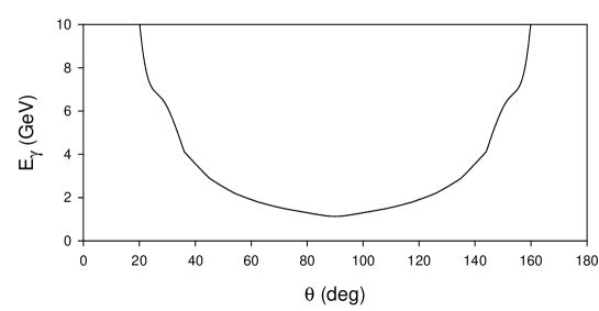
Figure 1: Angular dependence of the scale for large momentum transfer in deuteron photodisintegration.

For electrodisintegration, only the most recent data [17, 18] begins to reach this threshold.

Here we will focus on deuteron processes, including photodisintegration and electrodisintegration. For recent reviews of deuteron studies at high momentum transfer, see [19, 20, 16]. Elastic electron scattering data at high momentum transfer is presented in [21, 22, 23, 24, 25]. Recent photodisintegration data can be found in [26, 27, 28, 29], and for electrodisintegration data, in [30, 31, 32, 33, 17, 18]. Other analyses of deuteron processes include hidden-color contributions to deuteron form factors [34], the hard rescattering mechanism [35], quark-gluon strings [36], the Moscow NN potential [37], and AdS/QCD models [38, 39].

One recent experiment [17] used the 10.6 GeV electron beam at JLab and the Hall C spectrometers to measure electron scattering from a liquid deuterium target. The final electron and the proton were detected, with the kinematics restricted to the exclusive process $ed\rightarrow e^{\prime}pn$. One spectrometer measured the final electron at a nominal 12.2^∘ degrees from the beam direction, with a momentum of 8.5-9.1 GeV such that the recorded events had a distribution of momentum transfer squared reaching 5 GeV². The events studied were taken from a bin of 4.5$\pm$0.5 GeV² in the tail of the distribution; however, the nominal transfer was 4.2 GeV², because the majority of the events were in the lower half of the bin.

A second spectrometer measured the proton momentum at a range of angles to the beam direction, tuned to select events where the (missing) neutron had an angle relative to the direction of the momentum transfer that fell within a chosen bin. In the one-photon exchange approximation, which we assume, the momentum transferred is, of course, the photon momentum. The published neutron angles are binned at 35^∘, 45^∘ and 75^∘, with the first two selected to minimize final-state interactions. For our purposes, the importance of these two angles is that the momentum transferred to the neutron reaches 1 GeV in a zero-binding approximation, so that, rather than focus on the internal structure of the deuteron, we can consider the response to a large momentum transfer to all the nucleons involved and we can see that experiments may be approaching the threshold where our model can be applied.

The RNHA model is constructed in detail in Sec. II for two-nucleon processes. In the remainder of the paper, we consider various processes for the deuteron. In Sec. III, the form factors, structure functions, and tensor polarization observables of elastic electron scattering from the deuteron are obtained. Photodisintegration and electrodisintegration are analyzed in Secs. IV and V. Within the zero-binding approximation, elastic scattering and photodisintegration live at edges of the kinematic range of electrodisintegration and are essentially special cases that provide introductory examples. Section VI contains a summary of the results and suggestions for additional applications. Many details of the electrodisintegration helicity amplitudes are left to an appendix.

II Construction of the model

The basic process for a two-nucleon system to absorb a photon and exchange momentum between the nucleons is illustrated in Fig. 2. These diagrams are modeled on the primitive process of $\gamma^{*}ff\rightarrow ff$, with $f$ representing a point-like nucleon. The structure of each nucleon is then introduced by combining the Feynman amplitude for each diagram with the appropriate form factor for each nucleon, evaluated at the net momentum transfer for that nucleon. For a deuteron process in the zero-binding limit, the initial nucleons share the initial deuteron momentum $p$ equally, so that $p_{p}=p_{n}=p/2$. We also neglect the nucleon mass difference, setting $m_{p}=m_{n}\equiv m$. The distinction between different photon-absorption processes is then in the nature of the photon, being either real or virtual, and in the outcome for the final nucleons, bound as a deuteron or not.

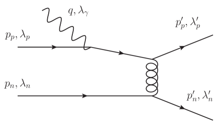
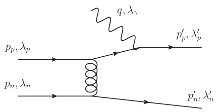
(a)	(b)
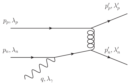
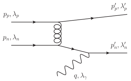
(c)	(d)

Figure 2: Tree graphs for deuteron processes that absorb a photon of momentum $q$ and helicity $\lambda_{\gamma}$. The initial (final) nucleon momentum and helicity are $p_{N}$ ($p^{\prime}_{N}$) and $\lambda_{N}$ ($\lambda^{\prime}_{N}$), with $N=p$ or $n$. The two nucleons exchange momentum via a vector particle. The four diagrams differ in the nature of the photon-absorbing nucleon and the order of this absorption and momentum transfer between nucleons.

The tree-level amplitudes for the four diagrams in Fig. 2 are

$$M_{a}^{\nu}(\lambda^{\prime}_{p},\lambda^{\prime}_{n},\lambda_{p},\lambda_{n}) = A_{p}^{\mu\nu}(p/2+q;\lambda^{\prime}_{p},\lambda_{p})\frac{1}{(p^{\prime}_{n}-p/2)^{2}}B_{n\mu}(\lambda^{\prime}_{n},\lambda_{n}),$$ (2)

$$M_{b}^{\nu}(\lambda^{\prime}_{p},\lambda^{\prime}_{n},\lambda_{p},\lambda_{n}) = A_{p}^{\nu\mu}(p^{\prime}_{p}-q;\lambda^{\prime}_{p},\lambda_{p})\frac{1}{(p^{\prime}_{n}-p/2)^{2}}B_{n\mu}(\lambda^{\prime}_{n},\lambda_{n}),$$ (3)

$$M_{c}^{\nu}(\lambda^{\prime}_{p},\lambda^{\prime}_{n},\lambda_{p},\lambda_{n}) = A_{n}^{\mu\nu}(p/2+q;\lambda^{\prime}_{n},\lambda_{n})\frac{1}{(p^{\prime}_{p}-p/2)^{2}}B_{p\mu}(\lambda^{\prime}_{p},\lambda_{p}),$$ (4)

$$M_{d}^{\nu}(\lambda^{\prime}_{p},\lambda^{\prime}_{n},\lambda_{p},\lambda_{n}) = A_{n}^{\nu\mu}(p^{\prime}_{n}-q;\lambda^{\prime}_{n},\lambda_{n})\frac{1}{(p^{\prime}_{p}-p/2)^{2}}B_{p\mu}(\lambda^{\prime}_{p},\lambda_{p}),$$ (5)

where

$$A_{N}^{\mu\nu}(p;\lambda^{\prime}_{N},\lambda_{N})=\bar{u}^{\prime}_{N}\gamma^{\mu}\frac{{\centernot{p}}+m}{p^{2}-m^{2}}\gamma^{\nu}u_{N},\;\;B_{N}^{\mu}(\lambda^{\prime}_{N},\lambda_{N})=\bar{u}^{\prime}_{N}\gamma^{\mu}u_{N},$$ (6)

with $u_{N}$ ($\bar{u}^{\prime}_{N}$) the initial (final) spinor for the nucleon $N$ with helicity $\lambda_{N}$ ($\lambda^{\prime}_{N}$). The sub-amplitude $A_{N}$ represents the fermion line that absorbs the photon, and $B_{N}$ represents the other fermion line. Calculation of these sub-amplitudes can be checked against the trace theorem for sums over helicities:

$$\sum_{\lambda_{N},\lambda^{\prime}_{N}}A_{N}^{\nu^{\prime}\mu^{\prime}*}(p;\lambda^{\prime}_{N},\lambda_{N})A_{N}^{\mu\nu}(p;\lambda^{\prime}_{N},\lambda_{N}) = {\rm Tr}\left[\gamma^{\nu^{\prime}}\frac{{\centernot{p}}+m}{p^{2}-m^{2}}\gamma^{\mu^{\prime}}({\centernot{p}}^{\prime}_{N}+m)\gamma^{\mu}\frac{{\centernot{p}}+m}{p^{2}-m^{2}}\gamma^{\nu}({\centernot{p}}_{N}+m)\right],$$

$$\sum_{\lambda_{N},\lambda^{\prime}_{N}}B_{N}^{\mu^{\prime}*}(\lambda^{\prime}_{N},\lambda_{N})B_{N}^{\mu}(\lambda^{\prime}_{N},\lambda_{N}) = {\rm Tr}\left[\gamma^{\mu^{\prime}}({\centernot{p}}^{\prime}_{N}+m)\gamma^{\mu}({\centernot{p}}_{N}+m)\right].$$ (8)

The full amplitude is constructed from the $M_{X}$ by combining them with form factors for each nucleon. For a deuteron with initial helicity $\lambda_{d}$, we have

$$M^{\nu}(\lambda^{\prime}_{p},\lambda^{\prime}_{n},\lambda_{d})=\sum_{\lambda_{p},\lambda_{n}}C_{\lambda_{p}\lambda_{n}}^{\lambda_{d}}\left[\sum_{X=a,b,c,d}M_{X}^{\nu}(\lambda^{\prime}_{p},\lambda^{\prime}_{n},\lambda_{p},\lambda_{n})\right]G_{p\lambda^{\prime}_{p}\lambda_{p}}(Q^{2}_{p})G_{n\lambda^{\prime}_{n}\lambda_{n}}(Q^{2}_{n}),$$ (9)

where $Q^{2}_{N}=-(p^{\prime}_{N}-p_{N})^{2}$,

$$C_{\lambda_{p}\lambda_{n}}^{\lambda_{d}}=\left\{\begin{array}[]{ll}\delta_{\lambda_{p}\pm\frac{1}{2}}\delta_{\lambda_{n}\pm\frac{1}{2}},&\lambda_{d}=\pm 1\\ \frac{1}{\sqrt{2}}\left(\delta_{\lambda_{p}\frac{1}{2}}\delta_{\lambda_{n}-\frac{1}{2}}+\delta_{\lambda_{p}-\frac{1}{2}}\delta_{\lambda_{n}+\frac{1}{2}}\right),&\lambda_{d}=0,\end{array}\right.$$ (10)

and

$$G_{N\lambda^{\prime}\lambda}=\left\{\begin{array}[]{ll}G_{EN},&\lambda^{\prime}=\lambda\\ G_{MN},&\lambda^{\prime}=-\lambda.\end{array}\right.$$ (11)

The form factors $G_{EN}$ and $G_{MN}$ represent the internal structure of the nucleons. They can be represented by data or empirical fits. For simplicity, we use the fits [40]

$$G_{Ep}\simeq\left(1+\frac{Q_{N}^{2}}{m_{0}^{2}}\right)^{-2},\;\;G_{Mp}\simeq\mu_{p}G_{Ep},\;\;G_{Mn}\simeq\mu_{n}G_{Ep},\;\;G_{En}\simeq-\frac{\mu_{n}\tau}{1+5.6\tau}G_{Ep},$$ (12)

where $m_{0}^{2}=0.71$ GeV², $\tau=\frac{Q_{N}^{2}}{4m^{2}}$, $\mu_{p}=2.79$, and $\mu_{n}=-1.91$. To limit the analysis to a single mass scale, we take the parameter $m_{0}$ to be proportional to the nuclear mass, with $m_{0}^{2}=0.80\,m^{2}$. We do not attempt to compute or assign an overall normalization to $M^{\nu}$, and the running of the strong coupling constant is not included.

The initial nucleon spinor, for a deuteron traveling along the negative $z$ direction, is [41]

$$u_{N}=\frac{{\centernot{p}}/2+m}{\sqrt{E_{d}/2+m}}\left(\begin{array}[]{c}\phi^{(\lambda_{N})}(-\hat{z})\\ 0\end{array}\right),$$ (13)

with

$$\phi^{(1/2)}(-\hat{z})=\left(\begin{array}[]{c}0\\ 1\end{array}\right),\;\;\phi^{(-1/2)}(-\hat{z})=\left(\begin{array}[]{c}1\\ 0\end{array}\right).$$ (14)

The final nucleon spinor is

$$u^{\prime}_{N}=\frac{{\centernot{p}}^{\prime}_{N}+m}{\sqrt{E^{\prime}_{N}+m}}\left(\begin{array}[]{c}\phi^{(\lambda^{\prime}_{N})}(\hat{p}^{\prime}_{N})\\ 0\end{array}\right),$$ (15)

with

$$\phi^{(1/2)}(\hat{p}^{\prime}_{N})=\left(\begin{array}[]{c}\cos(\theta_{N}/2)\\ e^{i\phi_{N}}\sin(\theta_{N}/2)\end{array}\right),\;\;\phi^{(-1/2)}(\hat{p}^{\prime}_{N})=\left(\begin{array}[]{c}-e^{-i\phi_{N}}\sin(\theta_{N}/2)\\ \cos(\theta_{N}/2)\end{array}\right),$$ (16)

where $\theta_{N}$ and $\phi_{N}$ are the polar and azimuthal angles of the outgoing momentum of the particular nucleon.

As discussed in the Introduction, the overall normalization of the RNHA amplitude is unknown. For comparison with data, we consider quantities which are themselves ratios or a ratio of the model to data.

III Elastic electron scattering

III.1 Form factors

The three deuteron form factors, $G_{C}$, $G_{M}$, and $G_{Q}$, are readily obtained from the hadronic helicity amplitudes of elastic electron-deuteron scattering in the Breit frame [42]. The kinematics are shown in Fig. 3. The photon four-momentum is $q=(0,0,0,q_{z})$ and the initial (final) deuteron four-momentum is $p=(E_{d},0,0,-q_{z}/2)$ ($p^{\prime}=(E_{d},0,0,q_{z}/2)$), with $q_{z}^{2}=Q^{2}$ and $E_{d}=\sqrt{Q^{2}/4+m_{d}^{2}}$. In the zero-binding limit, $m_{d}=2m$ and the individual nucleon four-momenta are $p_{p}=p_{n}=p/2$ and $p^{\prime}_{p}=p^{\prime}_{n}=p^{\prime}/2$. The hadronic matrix elements are given by

$$G_{\lambda^{\prime}_{d},\lambda_{d}}^{\mu}=\sum_{\lambda^{\prime}_{p},\lambda^{\prime}_{n}}C_{\lambda^{\prime}_{p}\lambda^{\prime}_{n}}^{\lambda^{\prime}_{d}}M^{\mu}(\lambda^{\prime}_{p},\lambda^{\prime}_{n},\lambda_{d}).$$ (17)

The initial spinors are as in (13); the final spinors are specified by

$$u^{\prime}_{N}=\frac{{\centernot{p}}^{\prime}/2+m}{\sqrt{E_{d}/2+m}}\left(\begin{array}[]{c}\phi^{(\lambda^{\prime}_{N})}(\hat{z})\\ 0\end{array}\right).$$ (18)

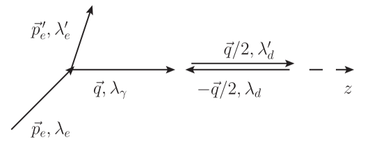
Figure 3: Kinematics for elastic electron-deuteron scattering in the Breit frame. The photon travels along the positive $z$ direction, and the deuteron comes from the right, along the negative $z$ direction.

The three form factors are then extracted as [42, 43]

$$G_{C}=\frac{-1}{2m_{d}\sqrt{1+\eta}}\frac{G_{00}^{+}-2G_{+-}^{+}}{3},\;\;G_{M}=\frac{2}{2m_{d}\sqrt{1+\eta}}\frac{G_{+0}^{x}}{\sqrt{2\eta}},\;\;G_{Q}=\frac{-1}{2m_{d}\sqrt{1+\eta}}\frac{G_{00}^{+}+G_{+-}^{+}}{2\eta},$$ (19)

with $\eta\equiv\frac{Q^{2}}{4m_{d}^{2}}$ and the $+$ superscript denoting the light-front sum of the 0 and $z$ components. For the helicity matrix elements, the model yields the following $Q^{2}$ dependence:

$$G_{00}^{+} = 0.5588{\cal N}m\left(\frac{m}{Q}\right)^{9}\left[1+129.1\frac{m^{2}}{Q^{2}}+{\cal O}(\frac{m^{4}}{Q^{4}})\right],$$ (20)

$$G_{+-}^{+} = -69.85{\cal N}m\left(\frac{m}{Q}\right)^{11}\left[1+4.8\frac{m^{2}}{Q^{2}}+{\cal O}(\frac{m^{4}}{Q^{4}})\right],$$ (21)

$$G_{+0}^{x} = 8.851{\cal N}m\left(\frac{m}{Q}\right)^{10}\left[1+4.8\frac{m^{2}}{Q^{2}}+{\cal O}(\frac{m^{4}}{Q^{4}})\right],$$ (22)

with ${\cal N}$ the unknown normalization. The factor of $m/Q$ associated with each helicity flip [44] is clearly evident. For the form factors, we find

$$G_{C} = -\frac{0.5588}{\sqrt{1+\eta}}\frac{{\cal N}}{12}\left(\frac{m}{Q}\right)^{9}\left[1+379.1\frac{m^{2}}{Q^{2}}+{\cal O}(\frac{m^{4}}{Q^{4}})\right],$$ (23)

$$G_{M} = \frac{8.851}{\sqrt{\eta(1+\eta)}}\frac{{\cal N}}{2\sqrt{2}}\left(\frac{m}{Q}\right)^{10}\left[1+4.8\frac{m^{2}}{Q^{2}}+{\cal O}(\frac{m^{4}}{Q^{4}})\right],$$ (24)

$$G_{Q} = -\frac{0.5588}{\eta\sqrt{1+\eta}}\frac{{\cal N}}{8}\left(\frac{m}{Q}\right)^{9}\left[1+4.086\frac{m^{2}}{Q^{2}}+{\cal O}(\frac{m^{4}}{Q^{4}})\right].$$ (25)

The leading $\pm$ signs are as expected for large $Q^{2}$.

We have left the kinematic factor $\eta=Q^{2}/16m^{2}$ without substitution, because there can be three regimes for $Q^{2}$. In addition to $Q^{2}$ large or small, there can be an intermediate region where $Q^{2}$ is large but $\eta$ is not. Such an intermediate regime does exist for $G_{M}$ and $G_{Q}$, where the coefficients of the nonleading terms are small enough for this correction to be small while $\eta$ is also small. For $G_{C}$, this is not the case, because the coefficient of the nonleading term is large enough to require a $Q^{2}$ value for which $\eta$ is also large. In the intermediate regime, we obtain

$$G_{M}\sim\left(\frac{m}{Q}\right)^{11},\;\;G_{Q}\sim\left(\frac{m}{Q}\right)^{11},$$ (26)

and for the large-$\eta$ regime

$$G_{C}\sim\left(\frac{m}{Q}\right)^{10},\;\;G_{M}\sim\left(\frac{m}{Q}\right)^{12},\;\;G_{Q}\sim\left(\frac{m}{Q}\right)^{12}.$$ (27)

Ratios of these form factors at very large $Q^{2}$ can be compared with the tree-level ratios for a point-like spin-one particle, such as the $W^{+}$, which are [43]

$$\frac{G_{C}}{G_{Q}}=\frac{2}{3}\eta-1,\;\;\frac{G_{M}}{G_{Q}}=-2.$$ (28)

Such behavior is immediately reproduced for form factors separated according to a Drell–Yan frame [45], with the assumption of strict $G^{+}_{00}$ dominance [43]. In terms of our hadronic matrix elements, we have

$$\frac{G_{C}}{G_{Q}}=\frac{2}{3}\eta-2\eta\frac{G^{+}_{+-}}{G^{+}_{00}+G^{+}_{+-}},\;\;\frac{G_{M}}{G_{Q}}=-2\sqrt{2\eta}\frac{G^{x}_{+0}}{G^{+}_{00}+G^{+}_{+-}}.$$ (29)

As already observed in [43], these Breit-frame ratios cannot both be resolved by simply assuming $G^{+}_{00}$ dominance. From our model, we obtain

$$\frac{G_{C}}{G_{Q}}=\frac{2}{3}\eta+15.6+{\cal O}(\frac{m^{2}}{Q^{2}}),\;\;\frac{G_{M}}{G_{Q}}=-11.2+{\cal O}(\frac{m^{2}}{Q^{2}}).$$ (30)

The leading $\frac{2}{3}\eta$ is just kinematic. The deviations of 15.6 and -11.2 from -1 and -2, respectively, are due to nonleading contributions multiplied by powers of $\eta$. Similar deviations will arise for calculations done in the Drell–Yan frame, because $\eta$ factors again interfere with strict $G_{00}^{+}$ dominance. Plots of these ratios are shown in Fig. 4.

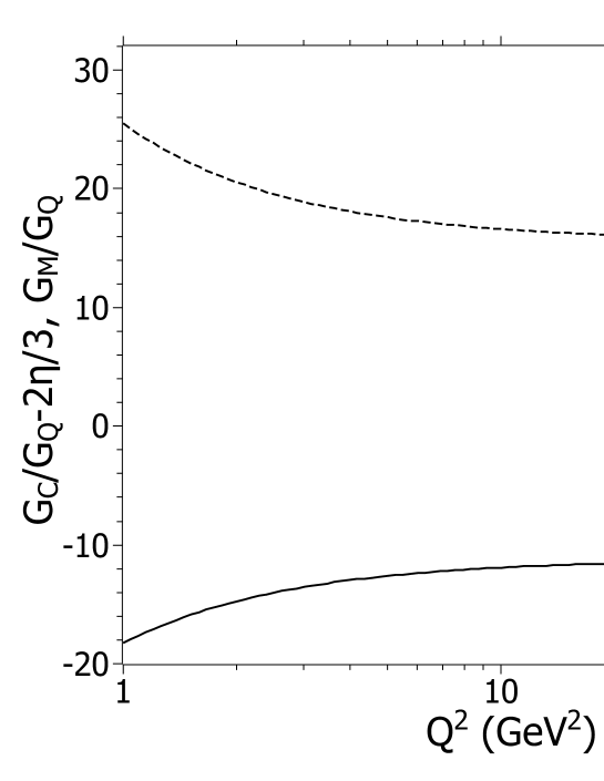
Figure 4: Ratios $G_{C}/G_{Q}-2\eta/3$ (dashed) and $G_{M}/G_{Q}$ (solid) for the model deuteron form factors.

III.2 Structure functions

Experiments designed to extract these form factors measure cross sections and polarization observables in elastic electron-deuteron scattering. The unpolarized cross section

$$\frac{d\sigma}{d\Omega}\propto S,\;\;S\equiv A(Q^{2})+B(Q^{2})\tan^{2}(\theta_{e}/2)$$ (31)

depends on the electron scattering angle $\theta_{e}$ and two structure functions

$$A(Q^{2}) \equiv G_{C}^{2}+\frac{8}{9}\eta^{2}G_{Q}^{2}+\frac{2}{3}\eta G_{M}^{2},$$ (32)

$$B(Q^{2}) \equiv \frac{4}{3}\eta(1+\eta)G_{M}^{2}.$$ (33)

These have been measured at the highest $Q^{2}$ yet attained at JLab [22, 23, 24], and $A$ has been measured at comparable $Q^{2}$ at SLAC [21]. However, these do not yet reach the $Q^{2}$ values needed for a definitive comparison. Figures 5 and 6 show plots of the data divided by the model, including an arbitrary normalization factor.

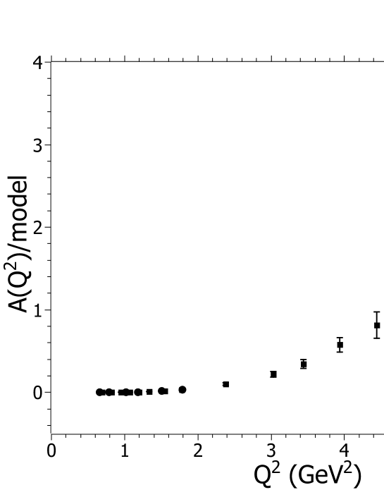
Figure 5: Data for the deuteron structure function $A(Q^{2})$ divided by the model function, including an arbitrary normalization. Experimental values are taken from [23] (circles) and [24] (squares).

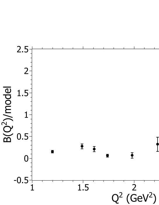
Figure 6: Data for the deuteron structure function $B(Q^{2})$ divided by the model function, including an arbitrary normalization. Experimental values are taken from [22].

In our model, expansions of these functions in inverse powers of $Q^{2}$ are

$$A(Q^{2}) = 0.1041{\cal N}^{2}\left(\frac{m}{Q}\right)^{20}\left[1+1246\frac{m^{2}}{Q^{2}}+{\cal O}(\frac{m^{4}}{Q^{4}})\right],$$ (34)

$$B(Q^{2}) = 13.06{\cal N}^{2}\left(\frac{m}{Q}\right)^{20}\left[1+9.6\frac{m^{2}}{Q^{2}}+{\cal O}(\frac{m^{4}}{Q^{4}})\right].$$ (35)

Because the expansion for $G_{C}$ is valid only for large $\eta$, we have used the explicit form of $\eta$ in constructing the expansion for $A$. The function $B$ is independent of $\eta$; the leading factor of $\eta(1+\eta)$ in its definition exactly cancels against factors in the relationship of $G_{M}$ to hadronic matrix elements. The expansion for $B$ converges much faster than the expansion for $A$, and the leading $Q^{2}$ behavior is dominant for $Q^{2}\gg 10$ GeV² only for $B$. For $A$, one must wait until impossibly large $Q^{2}$, which enters a regime where the collective quark substructure is important, including hidden-color effects [34], and the point-like approximation used in our model is invalid.

In [22] the large $Q^{2}$ behavior of $B$ is quoted as being $Q^{-24}$ from perturbative QCD. This faster fall off compared to $A$ is attributed to the extra suppression of the helicity flip involved in $G_{M}$. However, there are other compensating factors, and, just as in our model, the behavior of $B$ should be $Q^{-20}$, which is the same as $A$. In Fig. 7 we plot the ratio of $B$ to $A$ for a large range of $Q^{2}$. This ratio becomes constant at very large $Q^{2}$. Although the plots begin at low $Q^{2}$, there is nothing in the model that could reproduce diffractive minima, hence the smooth appearance.

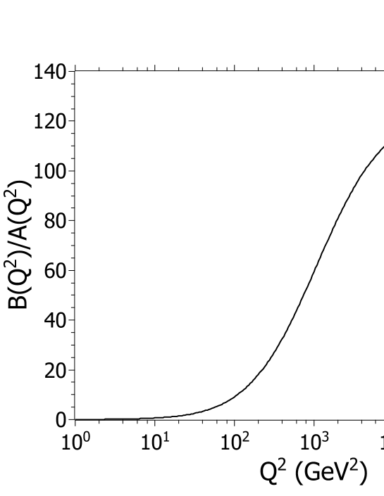
Figure 7: Ratio of $B$ to $A$ for the model deuteron structure functions.

III.3 Tensor polarization observables

Experiments can also extract tensor polarization observables [20, 25]

$$t_{20} \equiv -\frac{1}{\sqrt{2}S}\left[\frac{8}{3}\eta G_{C}G_{Q}+\frac{8}{9}\eta^{2}G_{Q}^{2}+\frac{1}{3}\eta\left(1+2(1+\eta)\tan^{2}(\theta_{e}/2)\right)G_{M}^{2}\right],$$ (36)

$$t_{21} \equiv \frac{2\eta}{\sqrt{3}S\cos(\theta_{e}/2)}\sqrt{\eta+\eta^{2}\sin^{2}(\theta_{e}/2)}G_{M}G_{Q},$$ (37)

$$t_{22} \equiv -\frac{\eta}{2\sqrt{3}S}G_{M}^{2}.$$ (38)

The highest $Q^{2}$ measurements of these were also done at JLab [25]. When $\eta$ is held explicit, expansions in $m/Q$ are

$$t_{20} = -\sqrt{2}+1064[1+2(1+\eta)\tan^{2}(\theta_{e}/2)]\left(\frac{m}{Q}\right)^{2}+{\cal O}(\frac{m^{4}}{Q^{4}}),$$ (39)

$$t_{21} = 38.8\sec(\theta_{e}/2)\sqrt{\eta+\sin^{2}(\theta_{e}/2)}\frac{m}{Q}$$

$$+\sec(\theta_{e}/2)\sqrt{\eta+\sin^{2}(\theta_{e}/2)}[48606+77869(1+\eta)\tan^{2}(\theta_{e}/2)]\left(\frac{m}{Q}\right)^{3}+{\cal O}(\frac{m^{4}}{Q^{4}}),$$

$$t_{22} = -434.5\left(\frac{m}{Q}\right)^{2}+[544703+872133(1+\eta)\tan^{2}(\theta_{e}/2)]\left(\frac{m}{Q}\right)^{4}+{\cal O}(\frac{m^{6}}{Q^{6}}).$$ (41)

While at very large $Q^{2}$, they are

$$t_{20} = -\sqrt{2}+133\tan^{2}(\theta_{e}/2)+1064[1+2\tan^{2}(\theta_{e}/2)]\left(\frac{m}{Q}\right)^{2}+{\cal O}(\frac{m^{4}}{Q^{4}}),$$ (42)

$$t_{21} = 1217\sec(\theta_{e}/2)\sin(\theta_{e}/2)[\tan^{2}(\theta_{e}/2)-0.007972]+\left[\right]\left(\frac{m}{Q}\right)^{2}+{\cal O}(\frac{m^{4}}{Q^{4}}),$$ (43)

$$t_{22} = -[434.5-54508\tan^{2}(\theta_{e}/2)]\left(\frac{m}{Q}\right)^{2}$$

$$+[544703+872133\tan^{2}(\theta_{e}/2)]\left(\frac{m}{Q}\right)^{4}+{\cal O}(\frac{m^{6}}{Q^{6}}).$$

The coefficients of nonleading terms are quite large. Thus, very large $Q^{2}$ is required for the leading term to be dominant, well beyond any available data. The limit of $-\sqrt{2}$ for $t_{20}$ at $\theta_{e}=0^{\circ}$ was an early prediction of perturbative QCD [46, 44]. However, as argued elsewhere [43], this value is obtained only at very large $Q^{2}$, and the value is quite different for small $\eta$. Figures 8 and 9 show plots of these observables at angles of 0^∘ and 30^∘, respectively. We also compare with data [25] in Figs. 10, 11, and 12. At these ‘small’ values of $Q^{2}$, only $t_{22}$ is consistent with data, something which is likely accidental with both data and model values near zero.

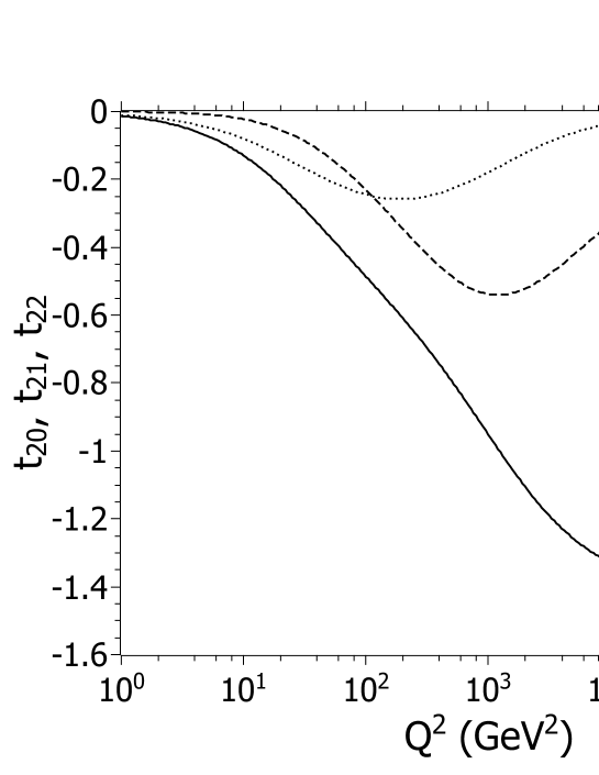
Figure 8: Deuteron tensor polarization observables $t_{20}$ (solid), $t_{21}$ (dashed), and $t_{22}$ (dotted) as computed in the model at an angle of $\theta_{e}=0^{\circ}$. The asymptotic value of $t_{20}(0^{\circ})$ is $-\sqrt{2}$, as predicted by perturbative QCD [46, 44].

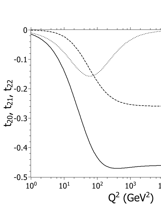
Figure 9: Same as Fig. 8 but for an angle of $\theta_{e}=30^{\circ}$.

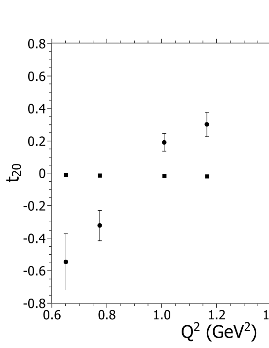
Figure 10: Plots of the tensor polarization observable $t_{20}$ of the deuteron from both data [25] (circles) and the model (squares) considered in the text. The angle $\theta_{e}$ varies and is as follows in order of increasing $Q^{2}$: 35.6^∘, 33.4^∘, 29.8^∘, 27.3^∘, 23.0^∘, and 19.8^∘.

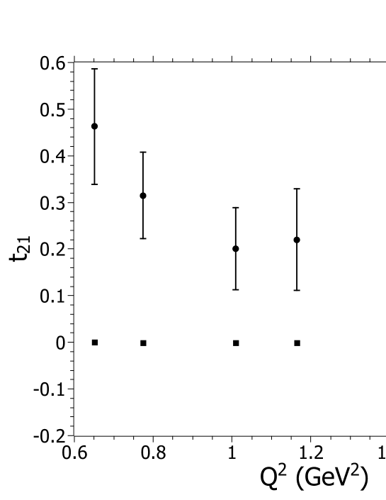
Figure 11: Same as Fig. 10 but for $t_{21}$.

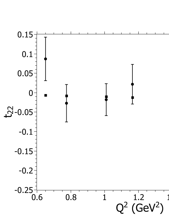
Figure 12: Same as Fig. 10 but for $t_{22}$.

IV Photodisintegration

In the photodisintegration of a deuteron, a real photon is absorbed and the two constituent nucleons emitted. This process is depicted in Fig. 13. The initial deuteron and photon four-momenta in the center-of-mass (c.m.) frame are $p=(E_{d},0,0,-q_{z})$ and $q=(q_{z},0,0,q_{z})$, where the incident photon is taken along the positive $z$ axis. The final proton and neutron four-momenta are $p^{\prime}_{p}=(E^{\prime}_{p},\vec{p}^{\,\prime}_{p})$ and $p^{\prime}_{n}=(E^{\prime}_{n},\vec{p}^{\,\prime}_{n})$, with $\theta_{p}$ and $\phi_{p}$ the polar and azimuthal angles of the final proton. By ignoring the nucleon mass difference, we have $E^{\prime}_{p}=E^{\prime}_{n}$, because momentum conservation guarantees $\vec{p}^{\,\prime}_{n}=-\vec{p}^{\,\prime}_{p}$ in the c.m. frame.

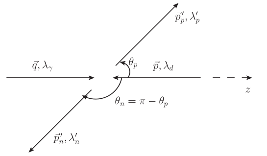
Figure 13: Kinematics for deuteron photodisintegration in the c.m. frame, with $\vec{q}$ the photon momentum and $\vec{p}=-\vec{q}$ the deuteron momentum. The final proton and neutron momenta are $\vec{p}^{\,\prime}_{p}$ and $\vec{p}^{\,\prime}_{n}$. The $\lambda$’s are helicities. Coordinates are chosen such that the photon enters along the positive $z$ direction and the azimuthal angle $\phi_{p}$ of the proton is zero.

In terms of the Mandelstam variable $s$, the c.m. energies and momenta are

$$E_{d}=(s+4m^{2})/(2\sqrt{s}),\;\;q_{z}=(s-4m^{2})/(2\sqrt{s}),\;\;E^{\prime}_{p}=\sqrt{s}/2,\;\;|\vec{p}^{\,\prime}_{p}|=\sqrt{s-4m^{2}}/2.$$ (45)

The photon energy in the lab frame is $E_{\gamma}=(s-4m^{2})/4m$. We will work at large $s$, so that momentum transfers are large.

The standard definition of helicity amplitudes for photodisintegration is [47]

$$F_{i\pm}\equiv\epsilon_{\nu}(\lambda_{\gamma})M^{\nu}(\lambda^{\prime}_{p},\lambda^{\prime}_{n},\lambda_{d})$$ (46)

with $\epsilon$ the polarization vector for a photon with helicity $\lambda_{\gamma}$ and $M^{\nu}$ given in (9). The index $i$ is associated with particular helicity combinations as follows:

$$F_{1\pm} = \epsilon_{\nu}(1)M^{\nu}(\pm\frac{1}{2},\pm\frac{1}{2},1),\;\;F_{2\pm}=\epsilon_{\nu}(1)M^{\nu}(\pm\frac{1}{2},\pm\frac{1}{2},0),$$ (47)

$$F_{3\pm} = \epsilon_{\nu}(1)M^{\nu}(\pm\frac{1}{2},\pm\frac{1}{2},-1),\;\;F_{4\pm}=\epsilon_{\nu}(1)M^{\nu}(\pm\frac{1}{2},\mp\frac{1}{2},1),$$ (48)

$$F_{5\pm} = \epsilon_{\nu}(1)M^{\nu}(\pm\frac{1}{2},\mp\frac{1}{2},0),\;\;F_{6\pm}=\epsilon_{\nu}(1)M^{\nu}(\pm\frac{1}{2},\mp\frac{1}{2},-1).$$ (49)

The other helicity combinations are related to these by parity.

The helicity amplitudes can be used to compute various polarization observables. The recoil-proton polarization $P_{y}$ measures the asymmetry parallel/antiparallel to the normal $\hat{y}\propto\vec{q}\times\vec{p}^{\,\prime}_{p}$ to the scattering plane:

$$P_{y}=2{\rm Im}\sum_{i=1}^{3}[F_{i+}^{\dagger}F_{i+3,-}+F_{i+3,+}^{\dagger}F_{i-}]/f(\theta),$$ (50)

where $f(\theta)=\sum_{i=1}^{6}[|F_{i+}|^{2}+|F_{i-}|^{2}]$ is the sum of all the helicity amplitudes squared. The transferred polarizations $C_{x^{\prime}}$ and $C_{z^{\prime}}$ measure asymmetries parallel/antiparallel to the $\hat{x}^{\prime}\propto\vec{p}^{\,\prime}_{p}\times\hat{y}$ and $\hat{z}^{\prime}=\hat{p}^{\,\prime}_{p}$ directions:

$$C_{x^{\prime}} = 2{\rm Re}\sum_{i=1}^{3}[F_{i+}^{\dagger}F_{i+3,-}+F_{i+3,+}^{\dagger}F_{i-}]/f(\theta),$$ (51)

$$C_{z^{\prime}} = \sum_{i=1}^{6}[|F_{i+}|^{2}-|F_{i-}|^{2}]/f(\theta).$$ (52)

The asymmetry $\Sigma$ for linearly polarized photons is given by

$$\Sigma=-2{\rm Re}\left[\sum_{\pm}(F_{1\pm}^{\dagger}F_{3\mp}-F_{4\pm}^{\dagger}F_{6\mp})-F_{2+}^{\dagger}F_{2-}+F_{5+}^{\dagger}F_{5-}\right]/f(\theta).$$ (53)

Each observable is formed as a ratio, which sets aside questions of normalization.

Because we only need to consider photons with helicity +1, the polarization vector is always $\epsilon=-\frac{1}{\sqrt{2}}(0,1,i,0)$, relative to the momentum in the positive $z$ direction. The final Dirac spinors are

$$u^{\prime}_{N}=\frac{{\centernot{p}}^{\prime}_{N}+m}{\sqrt{E^{\prime}_{N}+m}}\left(\begin{array}[]{c}\phi^{(\lambda^{\prime}_{N})}(\hat{p}^{\prime}_{N})\\ 0\end{array}\right),$$ (54)

with $\theta_{n}=\pi-\theta_{p}$, $\phi_{n}=\phi_{p}+\pi=\pi$, and

$$\phi^{(1/2)}(\hat{p}^{\prime}_{N})=\left(\begin{array}[]{c}\cos(\theta_{N}/2)\\ e^{i\phi_{N}}\sin(\theta_{N}/2)\end{array}\right),\;\;\phi^{(-1/2)}(\hat{p}^{\prime}_{N})=\left(\begin{array}[]{c}-e^{-i\phi_{N}}\sin(\theta_{N}/2)\\ \cos(\theta_{N}/2)\end{array}\right).$$ (55)

With these spinors as input, the amplitudes $\epsilon_{\nu}M_{X}^{\nu}$ can be evaluated in terms of Dirac matrix and spinor products and then combined to construct the predefined amplitudes $F_{i\pm}$. At large $s$, these RNHA predictions for the helicity amplitudes reduce to

$$F_{1+} \sim 4\frac{\sqrt{2}}{\sqrt{s}}{\rm csc}^{2}(\frac{\theta_{p}}{2})G_{En}(\theta_{p})G_{Ep}(\theta_{p}),\;\;F_{1-}\sim 0,$$ (56)

$$F_{2+} \sim 2\frac{m}{s}\cot^{3}(\frac{\theta_{p}}{2})[G_{En}(\theta_{p})G_{Mp}(\theta_{p})-G_{Mn}(\theta_{p})G_{Ep}(\theta_{p})],$$ (57)

$$F_{2-} \sim 2\frac{m}{s}\cot(\frac{\theta_{p}}{2})[G_{Mn}(\theta_{p})G_{Ep}(\theta_{p})-G_{En}(\theta_{p})G_{Mp}(\theta_{p})],$$

$$F_{3+} \sim 0,\;\;F_{3-}\sim 0,$$ (58)

$$F_{4+} \sim -4\sqrt{2}\frac{m}{s}\cot(\frac{\theta_{p}}{2})G_{Mn}(\theta_{p})G_{Ep}(\theta_{p}),\;\;F_{4-}\sim 4\sqrt{2}\frac{m}{s}\cot(\frac{\theta_{p}}{2})G_{En}(\theta_{p})G_{Mp}(\theta_{p}),$$ (59)

$$F_{5+} \sim \frac{2}{\sqrt{s}}\cot^{2}(\frac{\theta_{p}}{2})G_{En}(\theta_{p})G_{Ep}(\theta_{p}),\;\;F_{5-}\sim\frac{2}{\sqrt{s}}G_{En}(\theta_{p})G_{Ep}(\theta_{p}),$$ (60)

$$F_{6+} \sim 4\sqrt{2}\frac{m}{s}\cot^{3}(\frac{\theta_{p}}{2})G_{En}(\theta_{p})G_{Mp}(\theta_{p}),\;\;F_{6-}\sim-4\sqrt{2}\frac{m}{s}\cot(\frac{\theta_{p}}{2})G_{Mn}(\theta_{p})G_{Ep}(\theta_{p}).$$ (61)

From these we can calculate the various observables. Plots of the results and recent data [48, 49, 50] are given in Figs. 14, 15, 16, and 17. Because the tree-level amplitudes are real, $P_{y}$ is automatically zero. That $C_{x^{\prime}}$ is of order $m/\sqrt{s}$, rather than zero, is a correction to hadron helicity conservation [51]. Also, we find the asymmetry $\Sigma(90^{\circ})$ to be approximately -0.06, rather than the nominal expectation [52] of -1. In general, the trends with photon energy seem to be modestly consistent with data.

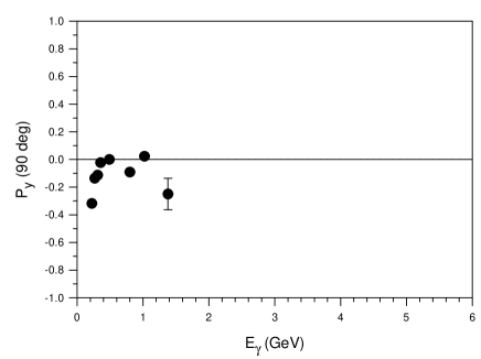
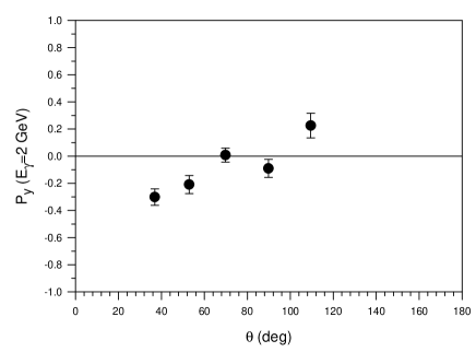
(a)	(b)

Figure 14: Recoil proton polarization $P_{y}$ as a function of (a) photon energy $E_{\gamma}$ and (b) proton angle $\theta$. For the latter, the photon energy is 2 GeV. The solid line is the RNHA prediction; the data points are from [48, 49].

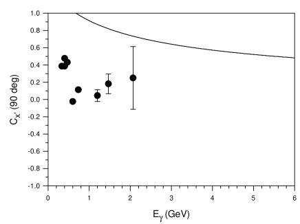
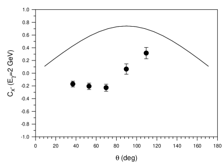
(a)	(b)

Figure 15: Same as Fig. 14 but for the transferred polarization $C_{x^{\prime}}$.

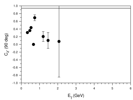
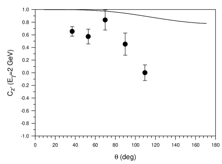
(a)	(b)

Figure 16: Same as Fig. 15 but for $C_{z^{\prime}}$.

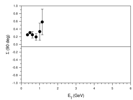
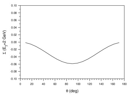
(a)	(b)

Figure 17: Same as Fig. 14 but for the asymmetry $\Sigma$. The data points are from [50].

V Electrodisintegration

The kinematics of the electrodisintegration process are shown in Fig. 18. The initial (final) momentum and helicity of the electron are $p_{e}$ ($p^{\prime}_{e}$) and $\lambda_{e}$ ($\lambda^{\prime}_{e}$). The intermediate photon carries four-momentum $q$. The azimuthal angle $\phi_{p}$ of the proton measures the rotation of the hadronic reaction plane relative to the electron scattering plane.

In the lab frame, with the $z$ axis taken along the photon three-momentum and the electron mass neglected, the initial and final electron four-momenta are

$$p_{e}=(E_{e},E_{e}\sin\theta_{e},0,E_{e}\cos\theta_{e}),\;\;p^{\prime}_{e}=(E^{\prime}_{e},E^{\prime}_{e}\sin\theta^{\prime}_{e},0,E^{\prime}_{e}\cos\theta^{\prime}_{e}),$$ (62)

with $E^{\prime}_{e}$ and $\tilde{\theta}=\theta^{\prime}_{e}-\theta_{e}$, the angle of the scattered electron to the beam direction, being measured. The photon four-momentum $q=(E_{\gamma},0,0,q_{z})$ is just $p_{e}-p^{\prime}_{e}$, which yields

$$Q^{2}\equiv-q^{2}=2E_{e}E^{\prime}_{e}(1-\cos\tilde{\theta}),\;\;E_{\gamma}=E_{e}-E^{\prime}_{e},\;\;q_{z}=\sqrt{E_{\gamma}^{2}+Q^{2}}.$$ (63)

The deuteron four-momentum is $p=(m_{d}=2m,0,0,0)$, and in the zero-binding limit, the initial proton and neutron four-momenta are $p_{p}=p_{n}=(m,0,0,0)$. The final nucleon four-momenta are

$$p^{\prime}_{p}=(E^{\prime}_{p}=\sqrt{\vec{p}^{\,\prime 2}_{p}+m^{2}},|\vec{p}^{\,\prime}_{p}|\sin\theta_{p}\cos\phi_{p},|\vec{p}^{\,\prime}_{p}|\sin\theta_{p}\sin\phi_{p},|\vec{p}^{\,\prime}_{p}|\cos\theta_{p}),$$ (64)

$$p^{\prime}_{n}=(E^{\prime}_{n}=\sqrt{\vec{p}^{\,\prime 2}_{n}+m^{2}},-|\vec{p}^{\,\prime}_{n}|\sin\theta_{n}\cos\phi_{p},-|\vec{p}^{\,\prime}_{n}|\sin\theta_{n}\sin\phi_{p},|\vec{p}^{\,\prime}_{n}|\cos\theta_{n}).$$ (65)

Within the one-photon-exchange approximation, the scattering amplitude is proportional to

$$M_{ed}(\lambda^{\prime}_{p},\lambda^{\prime}_{n},\lambda^{\prime}_{e};\lambda_{d},\lambda_{e})=\bar{u}^{\prime}_{e}\gamma_{\mu}u_{e}\frac{D_{\mu\nu}}{q^{2}}M^{\nu}(\lambda^{\prime}_{p},\lambda^{\prime}_{n},\lambda_{d}),$$ (66)

with $u_{e}$ ($u^{\prime}_{e}$) the initial (final) spinor of the electron and $M^{\nu}$ given in (9). The numerator of the photon progator is the sum over photon polarizations

$$D_{\mu\nu}=\sum_{\lambda=-1}^{1}(-1)^{\lambda}\epsilon_{\mu}^{*}(\lambda)\epsilon_{\nu}(\lambda).$$ (67)

The polarization four-vectors are

$$\epsilon(\pm 1)=\mp\frac{1}{\sqrt{2}}(0,1,\pm i,0),\;\;\epsilon(0)=(q_{z}/Q,0,0,E_{\gamma}/Q)$$ (68)

relative to the photon four-momentum $q=(E_{\gamma},0,0,q_{z})$. Polarization observables [5, 6, 7, 8, 9, 10, 11, 12, 13, 14, 15] can then be computed from these helicity amplitudes.

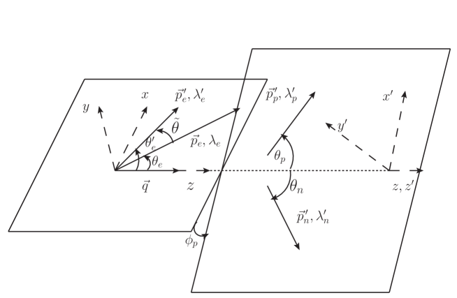
Figure 18: Kinematics for deuteron electrodisintegration. The unprimed axes are defined relative to the electron scattering plane, and the primed axes relative to the final nucleon momenta. The final proton momentum has polar angle $\theta_{p}$ and azimuthal angle $\phi_{p}$ relative to the unprimed frame.

In keeping with the notation of [6, 7] and [15], the differential cross section for electrodisintegration, summed over the final electron and neutron helicities in the lab frame, is [14, 15]

$$d\sigma \equiv \frac{d\sigma^{5}}{dE^{\prime}d\Omega^{\prime}_{e}d\Omega^{\prime}_{p}}$$

$$= \frac{m_{p}m_{n}|\vec{p}^{\,\prime}_{p}|}{16\pi^{3}m_{d}}\frac{\sigma_{\rm Mott}}{f_{\rm rec}}\left[\nu_{L}R_{L}+\nu_{T}R_{T}+\nu_{TT}R_{TT}+\nu_{LT}R_{LT}+2\lambda_{e}\nu_{LT^{\prime}}T_{LT^{\prime}}+2\lambda_{e}\nu_{T^{\prime}}R_{T^{\prime}}\right],$$

where $\Omega^{\prime}_{e}$ ($\Omega^{\prime}_{p}$) is the solid angle of the scattered electron (proton), $\sigma_{\rm Mott}$ is the Mott cross section, $f_{\rm rec}=|1+(E_{\gamma}|\vec{p}^{\,\prime}_{p}|-E^{\prime}_{p}q_{z}\cos\theta_{p})/(m_{d}|\vec{p}^{\,\prime}_{p}|)|$ is the lab recoil factor,

$$\nu_{L} = \frac{Q^{4}}{q_{z}^{4}},\;\;\nu_{T}=\frac{Q^{2}}{2q_{z}^{2}}+\tan^{2}\frac{\tilde{\theta}}{2},\;\;\nu_{TT}=\frac{Q^{2}}{2q_{z}^{2}},\;\;\nu_{LT}=\frac{Q^{2}}{\sqrt{2}q_{z}^{2}}\sqrt{\frac{Q^{2}}{q_{z}^{2}}+\tan^{2}\frac{\tilde{\theta}}{2}},$$ (70)

$$\nu_{LT^{\prime}} = -\frac{Q^{2}}{\sqrt{2}q_{z}^{2}}\tan\frac{\tilde{\theta}}{2},\;\;\nu_{T^{\prime}}=\tan\frac{\tilde{\theta}}{2}\sqrt{\frac{Q^{2}}{q_{z}^{2}}+\tan^{2}\frac{\tilde{\theta}}{2}},$$

and $\tilde{\theta}=\theta^{\prime}_{e}-\theta_{e}$ is the angle between the incoming and outgoing electron. The response functions $R_{X}$ depend upon the hadronic helicity amplitudes and the azimuthal angle $\phi_{p}$ of the hadronic scattering plane. The subscripts refer to the polarization of the intermediate photon, which enters on substitution of the polarization expansion (67) for the numerator of the photon propagator in the hadronic amplitude (66). The amplitude then decomposes into separate leptonic and hadronic factors

$$M_{ed}(\lambda^{\prime}_{p},\lambda^{\prime}_{n},\lambda^{\prime}_{e};\lambda_{d},\lambda_{e})=-\sum_{\lambda=-1}^{1}\bar{u}^{\prime}_{e}{\centernot{\epsilon}}^{*}(\lambda)u_{e}\frac{(-1)^{\lambda}}{Q^{2}}\epsilon_{\nu}(\lambda)M^{\nu}(\lambda^{\prime}_{p},\lambda^{\prime}_{n},\lambda_{d}).$$ (71)

The leptonic factors give rise to the $\nu_{X}$ coefficients, and the hadronic factors to the response functions in the square of the amplitude used to construct the cross section [15]. The subscript L(T) indicates a purely longitudinal (transverse) contribution, while LT is a cross term between longitudinal and transverse photon helicities. The TT subscript marks a cross term between different transverse helicities. A prime indicates a different combination of transverse helicities.

The response functions are computed from components of the hadronic tensor

$$w_{\lambda^{\prime},\lambda}=\frac{2}{3}\sum_{\lambda^{\prime\prime}_{p},\lambda^{\prime}_{p},\lambda^{\prime}_{n},\lambda^{\prime\prime}_{d},\lambda_{d}}\epsilon_{\nu}^{*}(\lambda^{\prime})M^{\nu*}(\lambda^{\prime\prime}_{p},\lambda^{\prime}_{n},\lambda^{\prime\prime}_{d})\rho^{p}_{\lambda^{\prime\prime}_{p},\lambda^{\prime}_{p}}\epsilon_{\mu}(\lambda)M^{\mu}(\lambda^{\prime}_{p},\lambda^{\prime}_{n},\lambda_{d})\rho^{d}_{\lambda^{\prime\prime}_{d},\lambda_{d}},$$ (72)

with $\rho^{p}$($\rho^{d}$) the density matrix for the proton (deuteron) helicity state. We construct these in the $xyz$ coordinate system of the electron scattering plane. The particular components are [6]

$$R_{L} = w_{0,0},\;\;R_{T}=w_{1,1}+w_{-1,-1},\;\;R_{T^{\prime}}=w_{1,1}-w_{-1,-1},$$ (73)

$$R_{TT} = 2{\rm Re}w_{1,-1},\;\;R_{LT}=-2{\rm Re}\left[w_{0,1}-w_{0,-1}\right],\;\;R_{LT^{\prime}}=-2{\rm Re}\left[w_{0,1}+w_{0,-1}\right].$$

For an unpolarized target, the deuteron density matrix is proportional to the identity, $\rho^{d}=\frac{1}{3}I$; similarly, if the proton helicity is not detected, $\rho^{p}=\frac{1}{2}I$. We then have the unpolarized cross section [6]

$$d\sigma_{\rm unpol}=\frac{m_{p}m_{n}|\vec{p}^{\,\prime}_{p}|}{16\pi^{3}m_{d}}\frac{\sigma_{\rm Mott}}{f_{\rm rec}}\sigma_{0},\;\;\sigma_{0}\equiv\nu_{L}R_{L}^{U}+\nu_{T}R_{T}^{U}+\nu_{TT}R_{TT}^{U}+\nu_{LT}R_{LT}^{U},$$ (74)

where the $R_{X}^{U}$ are computed with the simple density matrices. These are then computable in our model, with the basic computation being the evaluation of $\epsilon(\lambda_{\gamma})_{\mu}M^{\mu}$, which differs from the photodisintegration calculation in only two ways: $Q^{2}$ is not zero and $\lambda_{\gamma}$ ranges over all three possibilities.

The unpolarized response functions $R_{LT^{\prime}}^{U}$ and $R_{T^{\prime}}^{U}$ are identically zero. With $\rho^{d}$ replaced by $\frac{1}{3}I$ and the form (68) of the polarization vectors taken into account, ${\rm Re}w(0,1)$ is just the negative of ${\rm Re}w(0,-1)$, and $w_{1,1}$ is equal to $w_{-1,-1}$. Thus, the inputs to $R_{LT^{\prime}}^{U}$ and $R_{T^{\prime}}^{U}$, as given in (73), immediately cancel.

The recent $ed\rightarrow e^{\prime}pn$ experiment at JLab [17] does not include polarization but does begin to reach momentum transfers sufficient to consider the RNHA approach. Once polarization data is available, the expressions developed here and in the Appendix can be compared.

VI Summary

We have extended the reduced nuclear amplitude approach [1, 2] to helicity amplitudes and applied this model to analysis of elastic electron-deuteron scattering, deuteron photodisintegration, and deuteron electrodisintegration. These are just examples of the approach, which is generally applicable to exclusive nuclear processes. The primary limitation is that, for any process, the net momentum transfer to every nucleon must be large; therefore, as the number of nucleons increases, the required beam energy can increase dramatically. The primary gain is precocious scaling in the dependence on momentum transfer. What the model (or the original RNA approach) does not provide, though, is an overall normalization; comparisons must be made in terms of ratios.

By considering helicity amplitudes, many more quantities can be studied, including polarization dependence. All three of the deuteron’s electromagnetic form factors can be calculated and from there various elastic scattering observables can be constructed. In Sec. III we considered the standard structure functions $A$ and $B$ as well as the tensor polarizations $t_{2m}$. Generally, the model implies the need for momentum transfers larger than one would have hoped for seeing simple perturbative QCD scaling. However, our results do imply that the deuteron structure function $B$ is a good place to look, above a transfer of 10 GeV².

The RNHA results for polarization observables in deuteron photodisintegration, considered in Sec. IV, are somewhat consistent with experiment. In particular, our result for the asymmetry $\Sigma$, with a value of $\Sigma(90^{\circ})\simeq-0.06$, is much better than the value of -1 originally expected [52]. Higher photon energies would, of course, be useful.

We have also constructed the RNHA framework for analysis of deuteron electrodisintegration, in Sec. V. This stands ready for comparison with experiment when data is available at sufficient energies. One aspect that does remain is to consider polarization of the outgoing proton, in addition to polarization of the beam and target.

Other processes that one might consider include deeply virtual Compton scattering on the deuteron, pion photoproduction on the deuteron [3], and photodisintegration of ³He [4]. In each case, our approach can provide not only information about helicity amplitudes but also an analysis of nonleading momentum transfer dependence with respect to the onset of perturbative QCD scaling. We look forward to experiments at larger momentum transfers for all of these processes.

Appendix A Electrodisintegration with polarization

If we consider polarization for the beam and the target, the proton density matrix is still just $\rho^{p}=\frac{1}{2}I$, but the deuteron density matrix in the $xyz$ frame is [6]

$$\rho^{d}=\frac{1}{3}\left(\begin{array}[]{ccc}1+\sqrt{\frac{3}{2}}T_{10}+\frac{1}{\sqrt{2}}T_{20}&-\sqrt{\frac{3}{2}}(T_{11}^{*}+T_{21}^{*})&\sqrt{3}T_{22}^{*}\\ -\sqrt{\frac{3}{2}}(T_{11}+T_{21})&1-\sqrt{2}T_{20}&-\sqrt{\frac{3}{2}}(T_{11}^{*}-T_{21}^{*})\\ \sqrt{3}T_{22}&-\sqrt{\frac{3}{2}}(T_{11}-T_{21})&1-\sqrt{\frac{3}{2}}T_{10}+\frac{1}{\sqrt{2}}T_{20}\end{array}\right).$$ (75)

For a target polarization defined relative to the beam direction, rather than the $xyz$ system used above, the tensor polarization coefficients $T_{JM}$ are related to the coefficients $\tilde{T}_{JM}$ defined relative to the beam [6]. If only $\tilde{T}_{10}$ and $\tilde{T}_{20}$ are nonzero, the nonzero $T_{JM}$ are

$$T_{10} = \cos\tilde{\theta}\,\tilde{T}_{10},\;\;T_{11}=-\frac{1}{\sqrt{2}}\sin\tilde{\theta}\,\tilde{T}_{10},$$ (76)

$$T_{20} = \frac{1}{4}(1+3\cos 2\tilde{\theta})\tilde{T}_{20},\;\;T_{21}=-\sqrt{\frac{3}{8}}\sin 2\tilde{\theta}\,\tilde{T}_{20},\;\;T_{22}=\sqrt{\frac{3}{32}}(1-\cos 2\tilde{\theta})\tilde{T}_{20}.$$

The density matrix can then be written as

$$\rho^{d}=\left(\frac{1}{3}I+\tilde{T}_{10}\rho^{dV}+\tilde{T}_{20}\rho^{dT}\right),$$ (77)

where

$$\rho^{dV}=\frac{1}{3}\left(\begin{array}[]{ccc}\sqrt{\frac{3}{2}}\cos\tilde{\theta}&\frac{\sqrt{3}}{2}\sin\tilde{\theta}&0\\ \frac{\sqrt{3}}{2}\sin\tilde{\theta}&0&\frac{\sqrt{3}}{2}\sin\tilde{\theta}\\ 0&\frac{\sqrt{3}}{2}\sin\tilde{\theta}&-\sqrt{\frac{3}{2}}\cos\tilde{\theta}\end{array}\right)$$ (78)

and

$$\rho^{dT}=\frac{1}{3}\left(\begin{array}[]{ccc}\frac{1}{4\sqrt{2}}(1+3\cos 2\tilde{\theta})&\frac{3}{4}\sin 2\tilde{\theta}&\frac{3}{\sqrt{32}}(1-\cos 2\tilde{\theta})\\ \frac{3}{4}\sin 2\tilde{\theta}&-\frac{1}{2\sqrt{2}}(1+3\cos 2\tilde{\theta})&-\frac{3}{4}\sin 2\tilde{\theta}\\ \frac{3}{\sqrt{32}}(1-\cos 2\tilde{\theta})&-\frac{3}{4}\sin 2\tilde{\theta}&\frac{1}{4\sqrt{2}}(1+3\cos 2\tilde{\theta})\end{array}\right).$$ (79)

The response functions can then be separated into unpolarized, vector, and tensor contributions as $R_{X}=R_{X}^{U}+\tilde{T}_{10}R_{X}^{V}+\tilde{T}_{20}R_{X}^{T}$, with $R_{X}^{U}$, $R_{X}^{V}$, and $R_{X}^{T}$ computed with $\rho^{d}$ replaced by $\frac{1}{3}I$, $\rho^{dV}$, and $\rho^{dT}$, respectively.

With $d\sigma_{\rm unpol}$ defined as the unpolarized cross section, given in (74), the full cross section can be written as

$$d\sigma=\left[1+\tilde{T}_{10}\left(A_{d}^{V}+2\lambda_{e}A_{ed}^{V}\right)+\tilde{T}_{20}\left(A_{d}^{T}+2\lambda_{e}A_{ed}^{T}\right)\right]d\sigma_{\rm unpol},$$ (80)

in terms of the single and double asymmetries

$$A_{d}^{V} = \left[\nu_{L}R_{L}^{V}+\nu_{T}R_{T}^{V}+\nu_{TT}R_{TT}^{V}+\nu_{LT}R_{LT}^{V}\right]/\sigma_{0},$$ (81)

$$A_{ed}^{V} = \left[\nu_{LT^{\prime}}R_{LT^{\prime}}^{V}+\nu_{T^{\prime}}R_{T^{\prime}}^{V}\right]/\sigma_{0},$$ (82)

$$A_{d}^{T} = \left[\nu_{L}R_{L}^{T}+\nu_{T}R_{T}^{T}+\nu_{TT}R_{TT}^{T}+\nu_{LT}R_{LT}^{T}\right]/\sigma_{0},$$ (83)

$$A_{ed}^{T} = \left[\nu_{LT^{\prime}}R_{LT^{\prime}}^{T}+\nu_{T^{\prime}}R_{T^{\prime}}^{T}\right]/\sigma_{0}.$$ (84)

For a recent summary of data, see [54].

References

- [1] S.J. Brodsky and B.T. Chertok, The deuteron form-factor and the short distance behavior of the nuclear force, Phys. Rev. Lett. 37, 269 (1976); The asymptotic form-factors of hadrons and nuclei and the continuity of particle and nuclear dynamics, Phys. Rev. D 14, 3003 (1976).
- [2] S.J. Brodsky and J.R. Hiller, Reduced nuclear amplitudes in Quantum Chromodynamics, Phys. Rev. C 28, 475 (1983); 30, 412E (1984).
- [3] S. J. Brodsky, J. R. Hiller, C. R. Ji, and G. A. Miller, Perturbative QCD and factorization of coherent pion photoproduction on the deuteron, Phys. Rev. C 64, 055204 (2001).
- [4] S. J. Brodsky, L. Frankfurt, R. A. Gilman, J. R. Hiller, G. A. Miller, E. Piasetzky, M. Sargsian, and M. Strikman, Hard photodisintegration of a proton pair in 3He, Phys. Lett. B 578, 69 (2004).
- [5] S. Jeschonnek and J.W. Van Orden, Modeling quark-hadron duality in polarization observables, Phys. Rev. D 71, 054019 (2005); A new calculation for D at GeV energies, Phys. Rev. C 78, 014007 (2008).
- [6] S. Jeschonnek and J.W. Van Orden, Target polarization for at GeV energies, Phys. Rev. C 80, 054001 (2009).
- [7] S. Jeschonnek and J.W. Van Orden, Ejectile polarization for 2H at GeV energies, Phys. Rev. C 81, 014008 (2010).
- [8] W. P. Ford, S. Jeschonnek and J. W. Van Orden, 2H observables using a Regge model parameterization of final state interactions, Phys. Rev. C 87, 054006 (2013); Momentum distributions for 2H, Phys. Rev. C 90, 064006 (2014); S. Jeschonnek and J.W. Van Orden, Factorization breaking of for polarized deuteron targets in a relativistic framework, Phys. Rev. C 95, 044001 (2017).
- [9] J.M. Laget, The electro-disintegration of few body systems revisited, Phys. Lett. B 609, 49 (2005).
- [10] C. Ciofi delgi Atti and L.P. Kaptari, A non factorized calculation of the process 3HeH at medium energies, Phys. Rev. Lett. 100, 122301 (2008).
- [11] M.M. Sargsian, Large electrodisintegration of the deuteron in virtual nucleon approximation, Phys. Rev. C 82, 014612 (2010)
- [12] H. Arenhövel, W. Leidemann, and E.L. Tomusiak, General formulae for polarization observables in deuteron electrodisintegration and linear relations, Few Body Syst. 15, 109 (1993); General survey of polarization observables in deuteron electrodisintegration, Eur. Phys. J. A 23, 147 (2005).
- [13] G.I. Gakh, A.P. Rekalo, and E. Tomasi-Gustafsson, Relativistically invariant analysis of polarization effects in exclusive deuteron electrodisintegration process, Ann. Phys. 319, 150 (2005).
- [14] A.S. Raskin and T.W. Donnelly, Polarization in coincidence electron scattering from nuclei, Ann. Phys. 191, 78 (1989).
- [15] V. Dmitrasinovic and F. Gross, A Comment on general formulae for polarization observables in deuteron electrodisintegration and linear relations, Few Body Syst. 20, 41 (1996); Polarization observables in deuteron photodisintegration and electrodisintegration, Phys. Rev. C 40, 2479 (1989); 43, 1495E (1991).
- [16] C.E. Carlson, J.R. Hiller, and R.J. Holt, Relativistic QCD view of the deuteron, Ann. Rev. Nucl. Part. Sci. 47, 395 (1997).
- [17] C. Yero et al., Probing the deuteron at very large internal momenta, Phys. Rev. Lett. 125, 262501 (2020).
- [18] C. Yero, Cross Section Measurements of Deuteron Electro-Disintegration at Very High Recoil Momenta and Large 4-Momentum Transfers , Ph.D. thesis, Florida International University, Miami, Florida, 2020, [arXiv:2009.11343 [nucl-ex]].
- [19] W. Boeglin and M. Sargsian, Modern studies of the deuteron: From the lab frame to the light front, Int. J. Mod. Phys. E 24, 1530003 (2015).
- [20] R. A. Gilman and F. Gross, Electromagnetic structure of the deuteron, J. Phys. G 28, R37 (2002).
- [21] R.G. Arnold et al., Measurement of the electron-deuteron elastic-scattering cross section in the range GeV2, Phys. Rev. Lett. 35, 776 (1975).
- [22] P.E. Bosted et al., Measurements of the deuteron and proton magnetic form factors at large momentum transfers, Phys. Rev. C 42, 38 (1990).
- [23] D. Abbot et al., Precise measurement of the deuteron elastic structure function , Phys. Rev. Lett. 82, 1379 (1999).
- [24] L.C. Alexa et al., Measurements of the deuteron elastic structure function for (GeV/c)2 at Jefferson Laboratory, Phys. Rev. Lett. 82, 1374 (1999).
- [25] D. Abbot et al., Measurement of tensor polarization in elastic electron-deuteron scattering at large momentum transfer, Phys. Rev. Lett. 84, 5053 (2000).
- [26] C. Bochna et al., Measurements of deuteron photodisintegration up to 4.0 GeV, Phys. Rev. Lett. 81, 4576 (1998).
- [27] E.C. Schulte et al., Measurement of the high energy two-body deuteron photodisintegration differential cross section, Phys. Rev. Lett. 87, 102302 (2001).
- [28] E.C. Schulte et al., High energy angular distribution measurements of the exclusive deuteron photodisintegration reaction, Phys. Rev. C 66, 042201 (2002).
- [29] M. Mirazita et al,. Complete angular distribution measurements of two-body deuteron photodisintegration between 0.5 and 3 GeV, Phys. Rev. C 70, 014005 (2004).
- [30] W.-J. Kasdorp et al., Deuteron electrodisintegration at high missing momenta, Few Body Syst. 25, 115 (1998).
- [31] P.E. Ulmer et al., 2H reaction at high recoil momenta, Phys. Rev. Lett. 89, 062301 (2002).
- [32] W.U. Boeglin et al., Probing the high momentum component of the deuteron at high , Phys. Rev. Lett. 107, 262501 (2011).
- [33] K. S. Egiyan et al., Experimental study of exclusive 2H reaction mechanisms at high , Phys. Rev. Lett. 98 262502 (2007)
- [34] S.J. Brodsky, C.-R. Ji, and G.P. Lepage, Quantum Chromodynamic predictions for the deuteron form factor, Phys. Rev. Lett. 51, 83 (1983).
- [35] M.M. Sargsian, Polarization observables in hard rescattering mechanism of deuteron photodisintegration, Phys. Lett. B 587, 41 (2004).
- [36] V.Yu. Grishina et al, Forward-backward angle asymmetry and polarization observables in high-energy deuteron photodisintegration, Euro. Phys. J. A 19, 117 (2004).
- [37] V.A. Knyr, V.G. Neudachin, and N.A. Khokhlov, Description of polarization data for deuteron photodisintegration at photon energies in the range -2.5 GeV on the basis of the Moscow potential of NN interaction, Phys. Atom. Nucl. 70, 2152 (2007).
- [38] N. Huseynova, S. Mamedov, and J. Samadov, Deuteron electromagnetic form factors and tensor polarization observables in the framework of the hard-wall AdS/QCD model, [arXiv:2204.06205 [hep-ph]].
- [39] T. Gutsche, V. E. Lyubovitskij, I. Schmidt and A. Vega, Nuclear physics in soft-wall AdS/QCD: Deuteron electromagnetic form factors, Phys. Rev. D 91, 114001 (2015); T. Gutsche, V. E. Lyubovitskij and I. Schmidt, Deuteron electromagnetic structure functions and polarization properties in soft-wall AdS/QCD, Phys. Rev. D 94, 116006 (2016).
- [40] S. Glaster et al., Elastic electron-deuteron scattering and the electric neutron form factor at four-momentum transfers 5 fm 14 fm-2, Nucl. Phys. B 32, 221 (1971); M.A. Preston and R.K. Bhaduri, Structure of the nucleon, (Addison-Wesley,Reading, MA, 1975).
- [41] M.D. Scadron, Advanced quantum theory and its applications through Feynman diagrams, (Springer, Berlin, 1991).
- [42] R.G. Arnold, C.E. Carlson, and F. Gross, Elastic electron-deuteron scattering at high-energy, Phys. Rev. C 21, 1426 (1980).
- [43] S.J. Brodsky and J.R. Hiller, Universal properties of the electromagnetic interactions of spin one systems, Phys. Rev. D 46, 2141 (1992).
- [44] C. E. Carlson and F. Gross, ‘Smoking gun’ signatures for QCD in nuclear physics, Phys. Rev. Lett. 53, 127 (1984).
- [45] S.D. Drell and T.M. Yan, Connection of elastic electromagnetic nucleon form-factors at large and deep inelastic structure functions near threshold, Phys. Rev. Lett. 24, 181 (1970).
- [46] R. Dymarz and F.C. Khanna, Tensor polarization of the deuteron in elastic scattering, Phys. Rev. Lett. 56, 1448 (1986).
- [47] V.P. Barannik et al, Proton polarization in deuteron disintegration by linearly polarized photons and dibaryon resonances, Nucl. Phys. A 451, 751 (1986).
- [48] K. Wijesooriya et al., Polarization measurements in high-energy deuteron photodisintegration, Phys. Rev. Lett. 86, 2975 (2001).
- [49] X. Jiang et al., Recoil-proton polarization in high-energy deuteron photodisintegration with circularly polarized photons, Phys. Rev. Lett. 98, 182302 (2007).
- [50] F. Adamian et al., Measurement of the cross-section asymmetry of deuteron photodisintegration process by linearly polarized photons in the energy range GeV to 1.6 GeV, Eur. Phys. J. A 8, 423 (2000).
- [51] S.J. Brodsky and G.P. Lepage, Helicity selection rules and tests of gluon spin in exclusive QCD processes, Phys. Rev. D 24, 2848 (1981).
- [52] S.I. Nagornyi, Yu.A. Kasatkin, and I.K. Kirichenko, Photodisintegration of the deuteron at GeV in the model of asymptotic amplitudes, Sov. J. Nucl. Phys. 55, 189 (1992) [Yad. Fiz. 55, 345 (1992)].
- [53] D. Binosi, J. Collins, C. Kaufhold, and L. Theussl, JaxoDraw: A Graphical user interface for drawing Feynman diagrams. Version 2.0 release notes, Comput. Phys. Commun. 180, 1709 (2009); D. Binosi and L. Theussl, JaxoDraw: A Graphical user interface for drawing Feynman diagrams, Comput. Phys. Commun. 161, 76 (2004).
- [54] R. Mayer et al., Beam-target double-spin asymmetry in quasielastic electron scattering off the deuteron with CLAS, Phys. Rev. C 95, 024005 (2017).