HST Proper Motion Measurements of Supernova Remnant N132D: Center of Expansion and Age

Abstract

We present proper motion measurements of oxygen-rich ejecta of the LMC supernova remnant N132D using two epochs of Hubble Space Telescope Advanced Camera for Surveys data spanning 16 years. The proper motions of 120 individual knots of oxygen-rich gas were measured and used to calculate a center of expansion (CoE) of $\alpha$=$5^{h}25^{m}01.71^{s}$ and $\delta$=$-69^{\circ}38^{\prime}41\farcs 64$ (J2000) with a 1-$\sigma$ uncertainty of $2\farcs 90$. This new CoE measurement is $9\farcs 2$ and $10\farcs 8$ from two previous CoE estimates based on the geometry of the optically emitting ejecta. We also derive an explosion age of 2770 $\pm$ 500 yr, which is consistent with recent age estimates of $\approx 2500$ yr made from 3D ejecta reconstructions. We verify our estimates of the CoE and age using a new automated procedure that detected and tracked the proper motions of 137 knots, with 73 knots that overlap with the visually identified knots. We find the proper motions of ejecta are still ballistic, despite the remnant’s age, and are consistent with the notion that the ejecta are expanding into an ISM cavity. Evidence for explosion asymmetry from the parent supernova is also observed. Using the visually measured proper motion measurements and corresponding center of expansion and age, we compare N132D to other supernova remnants with proper motion ejecta studies.

1 Introduction

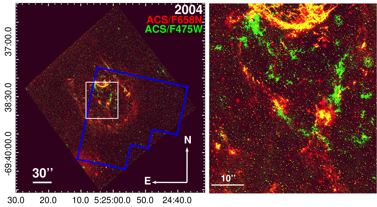
Figure 1: Left: Continuum subtracted image of N132D using images taken with HST/ACS and the F475W (green) and F658N (red) filters (additional image information can be found in Table 1). The blue polygon indicates the field of view of the 1994 WFPC2/F502N image. The white square is the cropped image of N132D used for proper motion measurements. Right: Enlarged view of the white square, highlighting in green the O-rich ejecta used for the proper motion measurements.

Supernova remnants (SNRs) provide valuable insights into the explosion processes of supernovae that are otherwise too distant to resolve (see Milisavljevic & Fesen, 2017, for a review). They offer unique opportunities to probe the elemental distribution of metal-rich ejecta and investigate the progenitor star’s mass loss history at fine scales (see Lopez & Fesen, 2018, for a review). Young, nearby oxygen-rich (O-rich) SNRs, created from the collapse of massive stars (ZAMS mass $>8M_{\odot}$; Smartt, 2009), are especially informative to study core-collapse dynamics because they are often associated with progenitor stars that were largely stripped of their hydrogen envelopes (e.g., Blair et al., 2000; Chevalier, 2005; Temim et al., 2022). The kinematic and chemical properties of their metal-rich ejecta retain information about the parent supernova explosion that would otherwise be lost in an H-rich explosion (Milisavljevic et al., 2010).

Tracking metal-rich ejecta over many years and measuring their proper motion enables estimates of the center of expansion (CoE) and explosion age, as well as information about the progenitor system’s circumstellar material (CSM) environment via ejecta interaction. The CoE and explosion age are important values for determining the kick velocity of compact objects (Vogt et al., 2018; Banovetz et al., 2021; Long et al., 2022), searching for surviving companions (Kerzendorf et al., 2019; Li et al., 2021), and measuring differences between optical and X-ray centers (Katsuda et al., 2018). These values can also serve as important tests for increasingly sophisticated 2D and 3D supernova simulations (e.g., Wongwathanarat et al., 2015; Janka et al., 2016; Burrows et al., 2019; Ferrand et al., 2021; Orlando et al., 2021, 2022).

Only a handful of known O-rich SNRs are sufficiently resolved to measure proper motion of high velocity ejecta from multi-epoch observations. This small list includes Cassiopeia A (Cas A; Kamper & van den Bergh, 1976; Thorstensen et al., 2001; Fesen et al., 2006; Hammell & Fesen, 2008), G292.0+1.8 (G292; Murdin & Clark, 1979; Winkler et al., 2009), and 1E 0102.2-7219 (E0102; Finkelstein et al., 2006; Banovetz et al., 2021). This paper focuses on the O-rich SNR N132D, which to date has no published proper motion measurements of its optically-emitting ejecta.

N132D is located in the bar of the Large Magellanic Cloud (LMC) and was first identified as a SNR from radio emission (Westerlund & Mathewson, 1966). Later, it was found to contain high velocity O-rich ejecta through optical spectra, classifying it as an O-rich SNR (Danziger & Dennefeld, 1976; Lasker, 1980). The parent supernova may have been a Type Ib with a 10-35 $M_{\odot}$ ZAMS progenitor (Blair et al., 2000; Sharda et al., 2020). Presently, the supernova continues to expand into a cavity created by the pre-supernova mass loss of the progenitor star (Hughes, 1987; Sutherland & Dopita, 1995; Blair et al., 2000; Chen et al., 2003; Sharda et al., 2020).

N132D is the brightest X-ray and gamma-ray SNR in the LMC (Clark, 1982; Favata et al., 1997; Borkowski et al., 2007; H. E. S. S. Collaboration et al., 2015; Ackermann et al., 2016). X-ray images show a horseshoe shaped forward shock (e.g., Borkowski et al., 2007; Bamba et al., 2018), the southern portion of which is associated with natal molecular clouds (Banas et al., 1997; Dopita et al., 2018; Sano et al., 2020). X-ray and radio observations indicate that N132D is transitioning from a young to middle-aged SNR and is about to enter the Sedov phase (Dickel & Milne, 1995; Favata et al., 1997; Bamba et al., 2018).

Table 1: HST Observations of N132D

PI	Date	Exp. Time	Instrument	Filter	$\lambda_{\rm center}$	Bandwidth	Pixel Scale
		(s)			(Å)	(Å)	(′′ pixel-1)
Blair	1994/08/09	3600	WFPC2/PC	F502N	5012	27	0.0455
Green	2004/01/22	1440	ACS/WFC	F658N	6584	75	0.049
Green	2004/01/22	1800	ACS/WFC	F550M	5580	389	0.049
Green	2004/01/21	1440	ACS/WFC	F775W	7702	1300	0.049
Green*	2004/01/22	1520	ACS/WFC	F475W	4760	1458	0.049
Milisavljevic*	2020/01/05	2320	ACS/WFC	F475W	4760	1458	0.049
Milisavljevic	2020/01/05	2480	WFC3/UVIS	F502N	5013	48	0.040

Note. — * denotes images used in proper motion analysis

Previous estimates of N132D’s explosion age have been made by dividing the radius of the SNR by the maximum radial velocity of the ejecta, yielding age estimates ranging from 1300-3440 yr (Danziger & Dennefeld, 1976; Lasker, 1980; Morse et al., 1995; Sutherland & Dopita, 1995). Morse et al. (1995) gave two estimates for the CoE of N132D. The first estimate was made by fitting an ellipse to the diffuse outer rim, and the second by finding the geometric center of O-rich ejecta. Recent 3D reconstructions of N132D use this geometrically-derived center as the CoE and find that N132D’s optically emitting oxygen-rich material is arranged in a torus distribution, inclined at an angle of $\approx 25-28^{\circ}$ in the plane of the sky (Vogt & Dopita, 2011; Law et al., 2020). They also provide the most recent age estimates of $\approx 2500$ yr.

This paper uses high resolution images obtained with the Hubble Space Telescope (HST) to measure proper motion of N132D’s oxygen-rich ejecta to estimate a CoE and explosion age. Section 2 discusses observations of N132D and the images used. Section 3 describes our proper motion measurements and analysis techniques. Section A introduces an automated procedure to measure proper motions using computer vision. Section 5 discusses the implications of the proper motion measurements, CoE, and explosion age as it pertains to previous estimates and other SNRs. We summarize and conclude in Section 6.

Figure 2: ACS/F475W images showing examples of the expanding ejecta knots in 2004 (left) and 2020 (right) in the area of the runaway knot (RK, see Section 5.1 for more details). The 2004 knot centroids are shown as yellow crosses while the 2020 centroids are shown as red crosses. The red arrow points in the direction of the CoE.

2 Observations

Using the Mikulski Archive for Space Telescopes (MAST) at the Space Telescope Science Institute, we examined three epochs of HST images that are sensitive to [O III] $\lambda\lambda$4959, 5007 emission tracing oxygen-rich ejecta of N132D. These consist of an image taken in 1994 using the Wide Field Planetary Camera 2 (WFPC2) with the F502N filter (PI: Blair GO-5365), a 2004 image using the the Advanced Camera for Surveys (ACS) and the F475W filter (PI: Green GO-12001), and a 2020 image using the ACS/F475W setup (PI: Milisavljevic GO-15818). The 1994 and 2020 F502N images use different instrument and filter configurations, whereas the 2004 and 2020 F475W images were both obtained with ACS. Utilizing the same camera/filter setup greatly improves the tracking confidence of the gas, as using different camera/filters setups can cause ambiguity in precise tracking due to brightening effects (see Banovetz et al., 2021). Thus, only the ACS images were used for proper motion tracking. The 2020 F502N image was used to confirm O-rich ejecta emission from possible continuum emission. All images were processed using Astrodrizzle (Gonzaga et al., 2012) and had a final image scale of approximately $0\farcs 05$ pixel^-1. Table 1 contains more information about the images used for analysis.

To align the images, we use the geomap task in PYRAF to create a transformation database using 30 anchor stars between the two images (see Table A1 in Appendix). These anchors were chosen for their low proper motions and small transformation residuals. The transformation had resulting residuals of $\approx 0.3$ pixels ($\approx 0\farcs 015$). We then used the PYRAF task geotran to apply this transformation, aligning the images. Once the images were aligned, they were cropped to a $51\farcs 5\times 58\farcs 3$ field of view that contains only the O-rich portion of the remnant (see Figure 1). The cropping extent was determined by visual examination of oxygen emission, and we ensured that all high proper motion ejecta knots were contained within the selected field of view. The World Coordinate System (WCS) was calculated using a locally compiled version of the Astrometry.net (Lang et al., 2010). This WCS solution is accurate to $\approx 0\farcs 17$ and was taken into account for the final CoE error.

3 Proper Motion Measurements: Manual Estimation

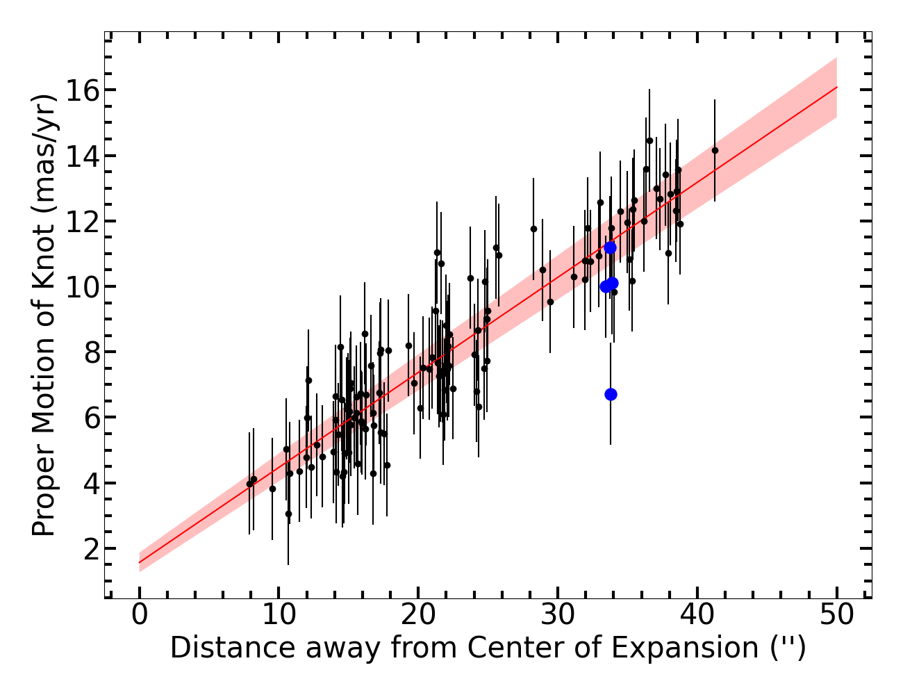
Figure 3: The absolute proper motion vs radial distance of the knots. The proper motions of the knots of ejecta are shown as black points with their corresponding 1-$\sigma$ error. The red line indicates a linear fit to the data with the shaded region indicating the 1-$\sigma$ error. The location of the four knots in the RK region are highlighted as blue points.

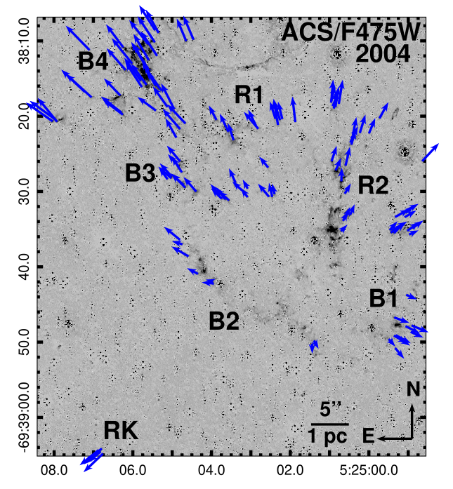
Figure 4: 2004 ACS/F475W continuum- and hydrogen-subtracted image with vectors representing the measured shifts (multiplied by a factor of 20 for visual clarity) shown in blue. The regions identified in Morse et al. (1995) are also labeled.

Using the aligned images, we identified knots with high proper motions. Knots were chosen by how well they could be tracked visually, with most knots being optically bright and circular to have confidence in the measurements. The shifts of the knots were calculated by blinking between the two images in SAOImage DS9 and visually locating the centers of the knots or other conspicuous features (see Figure 2). The centers were measured multiple times to estimate positional errors of each knot. During the 16 yrs, knots can possibly brighten/dim or change morphology as they interact with the surrounding medium (Fesen et al., 2011; Banovetz et al., 2021). This interaction can skew results if using the astrometric approach of fitting a Gaussian for the knots. We did apply a Gaussian based centroid fitting procedure (see Appendix and Section 4) and found more accurate results through manual inspection.

We applied our methodology to 120 knots (see Table A2 in Appendix), which resulted in proper motions ranging from 3–14.5 miliarcseconds (mas) per year, with a median proper motion of 7.54 mas yr^-1 and average relative error of $13\%$ (Figure 3). This translates to a median velocity of 1784 km s^-1 assuming a distance to the LMC of 50 kpc (Panagia et al., 1991). Our median velocity is consistent within uncertainties to the average expansion velocity of 1745 km s^-1 calculated using a fitted projected radius of N132D (Law et al., 2020). The linear fit also gives a higher scaling factor $S$ of $0\farcs 014$ per km s^-1 compared to $0\farcs 010$ per km s^-1 of Law et al. (2020). Figure 4 shows the locations and proper motions of the 120 knots, as well as the O-rich regions discussed in Morse et al. (1995).

3.1 Center of Expansion

Our approach to determine the CoE of N132D uses the trajectories of the ejecta augmented with a likelihood function. This method is similar to that used by Banovetz et al. (2021) and Thorstensen et al. (2001) for the calculation of E0102’s and Cas A’s CoE, respectively. We favor this method because it only depends on the direction of the knots, and is not sensitive to deceleration over time.

We assume that the likelihood of the CoE in the plane of sky coordinates (X,Y) is given by:

$$\mathcal{L}(X,Y)=\Pi_{i}\frac{w_{i}}{2\sigma_{i}}exp(-d^{2}_{i\perp}/(2\sigma_{i}^{2}))$$ (1)

$$w_{i}=\frac{1}{P_{y_{i}}P_{x_{i}}},$$ (2)

where $d_{i\perp}$ is the perpendicular distance between (X,Y) and the knot’s line of position, and $\sigma_{i}$ is the uncertainty associated with the point common to the knot’s extended line of position and $d_{i\perp}$ (Banovetz et al., 2021). We also define $w$, the probability of finding an individual knot in a given X and Y position, denoted by $P_{x_{i}}$ and $P_{y_{i}}$, respectively, which was calculated using a kernel density estimate (KDE) to fit knots in the (X,Y) plane. The (X,Y) combination that maximizes this function gives the CoE. The uncertainty of the CoE is derived from 100,000 artificial data sets generated from position and direction distributions of individual knots.

A notable difference from Banovetz et al. (2021) is the addition of a weight, $w$. We used this weight to minimize the effects of selection bias in our sample. As seen in Figure 4, N132D is unique compared to other O-rich SNRs in that the knot distribution is skewed, with a larger number of knots displaying proper motions in the northern region of the remnant as compared to the southern region. Without the weight, the CoE will skew in the direction of the more populated region. This added weight term compensates for sparse regions by giving proportionally more weight to knots in these regions.

Applying this procedure to our proper motion measurements yields a CoE of $\alpha$=5^h25^m01.71^s and $\delta$=-69^∘38^′$41\farcs 64$ (J2000) with a 1-$\sigma$ uncertainty of $2\farcs 90$. Figure 5 shows the trajectories of the knots as compared to the derived CoE.

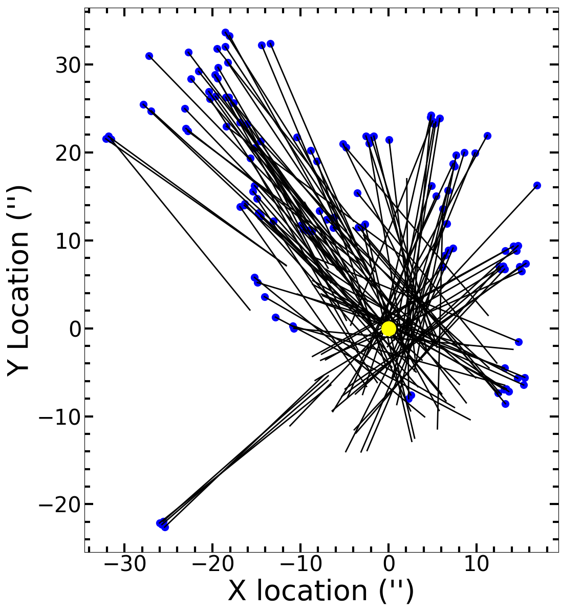
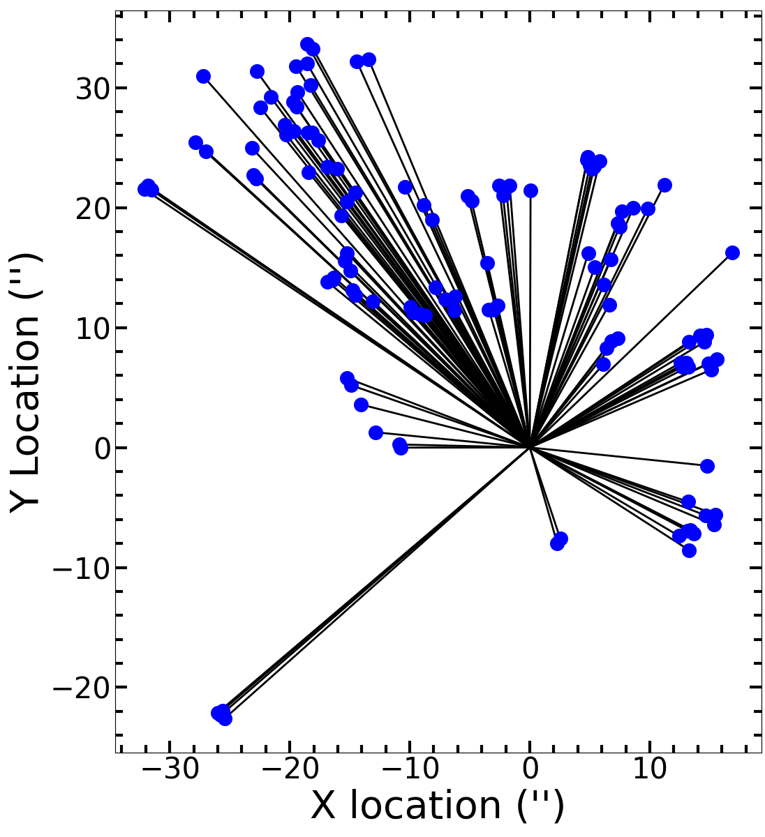
Figure 5: Left: The visually measured proper motions of the 120 knots traced back 25^′′ ($\approx$3000 yr assuming an average proper motion of 8.1 mas yr^-1 ). The CoE is shown in yellow. Right: The trajectories of the visually measured knots if forced to originate from our calculated CoE. Strong spatial asymmetry in the knot distribution is observed with respect to the CoE.

3.2 Explosion Age

Using the manually tracked knots and the associated center of expansion estimate, we calculated the explosion age of N132D by dividing the knot’s distance from the CoE by their proper motion measurements. Figure 6 shows the calculated explosion age of all 120 knots. Combining these ages resulted in an age of 2770 $\pm$ 500 yr.

We also calculated the explosion age using only the knots with the fastest proper motions. A similar approach was used by Fesen et al. (2006) for the explosion age of Cassiopeia A and Banovetz et al. (2021) for E0102. This method assumes that knots with the fastest proper motions are least decelerated, resulting in a more accurate explosion age. Forty-nine of the 120 knots with proper motions greater than the average (8.1 mas yr^-1 ) were selected. Almost all these knots correspond to the region B4 from Morse et al. (1995). Using these knots resulted in an explosion age of 2745 $\pm$ 404 yr, consistent with the age using all of the knots. For further discussion, we adopt the age of 2770 $\pm$ 500 yr, as this age is representative of all the knots.

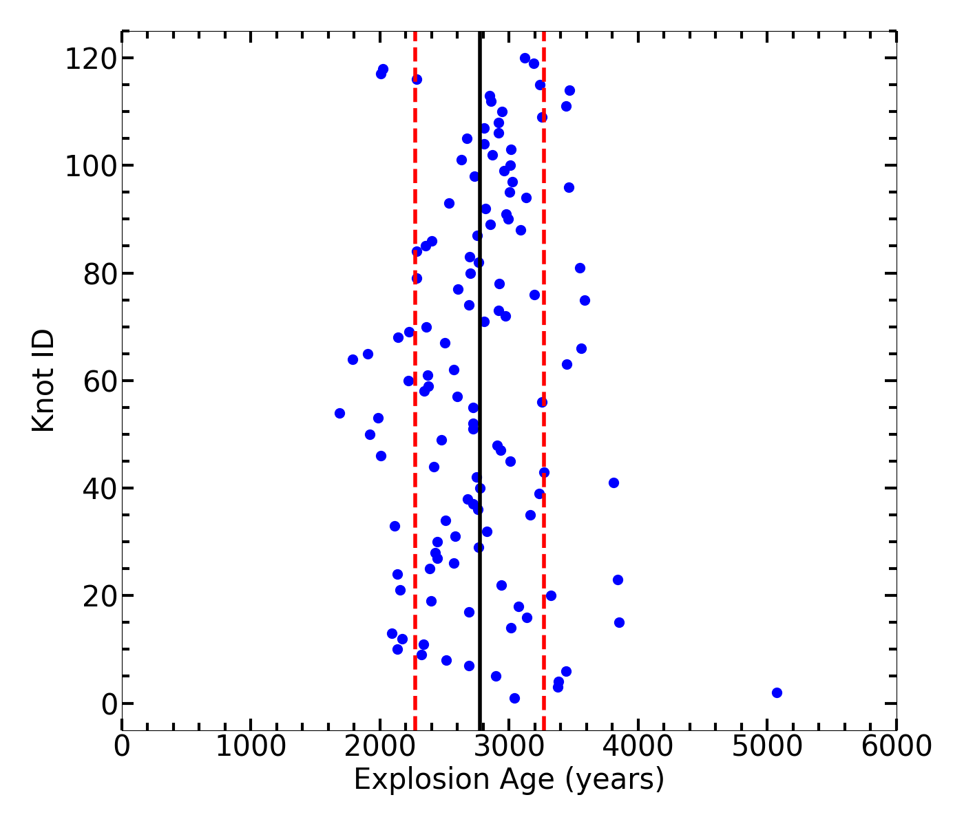
Figure 6: A comparison of the explosions age measurements, assuming our CoE. The black line represents the average age of the data set, while the red dashed line is the 1-$\sigma$ uncertainty. This results in an explosion age of 2770 $\pm$ 500 yr.

4 Proper Motion Measurements: Automated via Computer Vision

We also implemented a novel computer vision based approach to measure the proper motions of the ejecta. This approach utilizes hydrogen and continuum subtracted images between the epochs to insure that only the O-rich material is being tracked. Then, regions of high emission and/or high ejecta proper motions are specified. These regions, or stamps, are passed through an automated detection procedure to identify knots using image segmentation and deblending. To track the knots, a kernel density estimate (KDE) estimates the peaks within these segments, and we use these peaks to measure the proper motion between the epochs. A more detailed explanation of this procedure can be found in the Appendix.

The automated procedure identified and measured the proper motions of 137 knots of ejecta. Seventy-three of these 137 knots matched visually identified knots used in the manual procedure. The average difference in inferred values between the manual and automated procedures for the shift between epochs is $0\farcs 03$ (or $\approx 1.8$ mas yr^-1 ) and the vector angle is $\approx 12^{\circ}$. The error of the proper motions was set to 0.4 pixels ($\approx 0\farcs 2$), from the sub-pixel ratio of the KDE. While the automated proper-motion measurements generally followed the same ballistic $v\propto r$ relationship found with the visually tracked knots, the measurements exhibited more scatter and higher uncertainty. This discrepancy most likely arises from tracking fainter, less dense knots that are more susceptible to deceleration compared to the bright, denser knots that were found visually.

While our automated procedure generally produces similar results to the visually measured proper motions, the sample is contaminated by the less dense knots, possibly skewing the results. Hence, we adopt the visual measurement results for this paper. We note that, the results above used conservative metrics in the measurement of the proper motions in order to not be biased too heavily by any one parameter. Attempts to improve the results by fine-tuning these parameters can be found in the Appendix.

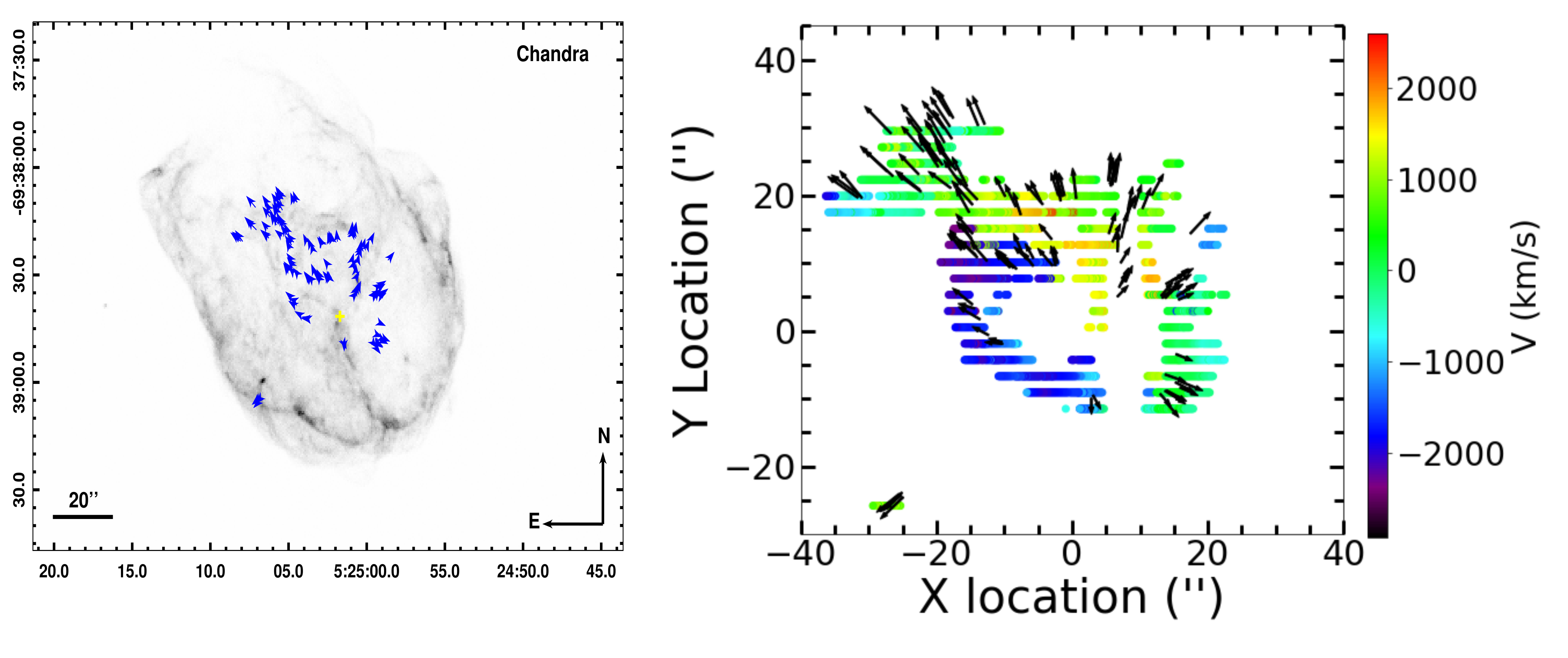
Figure 7: Left: Chandra image of N132D (PI: Borkowski). The proper motions from the visual measurements are in blue and our calculated CoE in yellow (see Section 3.1). Right: Vectors of proper motions (black) with Doppler velocities (Law et al., 2020), centered on our CoE (see Section 3.1).

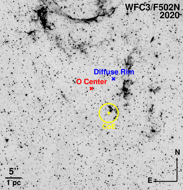
Figure 8: Center of expansion estimates for N132D. This paper’s CoE calculations and associated 1-$\sigma$ uncertainty is shown in yellow. This CoE is centered at $\alpha$=$5^{h}25^{m}01.71^{s}$ and $\delta$=$-69^{\circ}38^{\prime}41\farcs 64$ (J2000) with a 1-$\sigma$ uncertainty of $2\farcs 90$ and is $9\farcs 2$ and $10\farcs 8$ away from the estimates of Morse et al. (1995) found by fitting an ellipse to the diffuse outer rim (blue) and the O-rich geometric center (red).

5 Discussion

5.1 Proper Motion Measurements

Our work presents the first proper motion measurements of the O-rich ejecta of N132D. We visually identified and tracked 120 knots of ejecta across 16 years. While the baseline is large and could be on the order of shock cooling times, we are confident in our tracking ability. This is because the emission mechanism is most likely a combination of shock excitation and photoionization producing a high amount of [O III] emission (Sutherland & Dopita, 1995), the low densities of the shock will increase the cooling times (Blair et al., 2000), and we find similar morphology in the knots between epochs. With these 120 knots, we find that the ejecta follow homologous expansion with an average proper motion of 8.1 mas yr^-1 (median proper motion of 7.54 mas yr^-1 ) despite N132D’s advanced age approaching the Sedov phase.

Figure 3 shows the proper motions of the knots versus their distance away from our calculated CoE (see Section 3.1). Comparing this with spectroscopic measurements, the highest proper motion measurements are seen in the B4 region, as first reported in Morse et al. (1995), and shown in the left panel of Figure 4. This is to be expected, as B4 corresponds to a region of small Doppler velocities in the O-rich ejecta (Morse et al., 1995; Vogt & Dopita, 2011; Law et al., 2020), as seen in the upper left of the plot in the right panel of Figure 7. We find this inverse relationship between the proper motion measurements and Doppler velocities to hold true except for the region B1. B1 also corresponds to an area of small Doppler velocities, but the proper motion measurements are much smaller compared to B4. This difference in proper motions could be a result of B1 possibly being outside the reverse shock, as proposed by Vogt & Dopita (2011) (see Figure 7 for X-ray emission tracing the shocks). However, as this region is consistent with the ballistic trend, it is more likely associated with an explosion asymmetry (see Section 5.3 for more discussion).

Notably, the fit shown in Figure 3 does not pass through the origin and has an offset of $\approx+1.6$ mas yr^-1 . Forcing the line through the origin results in $S\approx 0\farcs 012$ per km s^-1 , which is closer to the value reported in Law et al. (2020). This offset in the original fit could be indicative of deceleration experienced by the ejecta over time. As the ejecta expands in the surrounding environment, the fastest ejecta will interact and decelerate at a different rate compared to the slower ejecta. This will disrupt the $v\propto r$ relation between ejecta velocity and distance from the CoE, introducing a positive offset term to the linear fit.

Table 2: Characteristics of Young O-rich SNRs

Parameter	G292	E0102	Cas A	N132D
Proper motion derived CoE (J2000)	11:24:34.4 [1]	1:04:02.48 [2]	23:23:27.77 [3]	5:25:01.71a
	-59:15:51	-72:01:53.92	+58:48:49.4	-69:38:41.64
CoE 1-$\sigma$ Error (′′)	5	1.77	0.4	2.90
Center of X-ray emission (J2000)	11:24:33.1 [4]	01:04:1.964 [5]	23:23:27.9 [4]	5:25:03.08b
	-59:15:51.1	-72:01:53.47	58:48:56.2	-69:38:32.6
Current Age (yr)	$\sim$2990 [1]	$\sim$1740 [2]	$\sim$350 [3]	$\sim$2770a
Distance to Remnant (kpc)	$6.2\pm 0.9$ [7]	$62.1\pm 1.9$ [8,9]	3.4 ${}^{+0.3}_{-0.1}$ [10]	$50.1\pm 3.1$ [11]
Size of Remnant (arcmin)	8.4–9.6 [12]	0.7 [5]	5.6 [13]	1.8 [14]
Ejecta transverse velocity (km/s)	$\sim$1500-3600 [1]	$\sim$1300–2700 [2]	$\sim$5500–14500 [15]	$\sim$700–3400a
Progenitor ZAMS Mass ($M_{\odot}$)	13–30 [16]	25–50 [17,18]	15–20 [19]	10–35 [17,20]

References. — [1] Winkler et al. (2009), [2] Banovetz et al. (2021), [3] Thorstensen et al. (2001), [4] Katsuda et al. (2018), [5] Xi et al. (2019), [6] Dickel & Milne (1995), [7] Gaensler & Wallace (2003), [8] Graczyk et al. (2014), [9] Scowcroft et al. (2016), [10] Reed et al. (1995), [11] Panagia et al. (1991), [12] Park et al. (2007), [13] Vink et al. (2022), [14] Law et al. (2020), [15] Fesen et al. (2006), [16] Bhalerao et al. (2019), [17] Blair et al. (2000), [18] Finkelstein et al. (2006), [19] Lee et al. (2014), [20] Sharda et al. (2020)

Figure 9: Locations of O-rich knots (blue) from N132D (this work), E0102 (Banovetz et al., 2021), Cas A (Hammell & Fesen, 2008), and G292 (Winkler et al., 2009), with trajectories (black) forced to originate on their proper-motion derived CoEs (Thorstensen et al., 2001; Winkler et al., 2009; Banovetz et al., 2021). Cas A also includes nitrogen rich knots (green) and fast moving knots (yellow) (Hammell & Fesen, 2008). The circle in the bottom right is 1 pc in radius. The physical distances were calculated using distance estimates and CoEs from Table 5.1.

A unique feature of N132D is the runaway knot (RK), which is an isolated small clump of ejecta located in the southwestern portion of the remnant and is unique in that it is enhanced in Si and S but not O (Law et al., 2020). The RK was first reported in Morse et al. (1995) and recent 3D reconstructions show that the knot is perpendicular to the main torus (Vogt & Dopita, 2011; Law et al., 2020). Explanations for the origin of the RK include evidence of a polar jet (Vogt & Dopita, 2011) and high velocity ejecta, similar to Cas A (Fesen & Gunderson, 1996; Law et al., 2020). We were able to find and measure the proper motions of four O-rich knots in the same region as the RK (see Figure 2 and Figure A2). The proper motions are faster than the global average but are still consistent with proper motions of other knots ($\approx 9.5$ mas yr^-1 or $\approx 2250$ km s^-1 ). Combining this with a Doppler velocity of 820 km s^-1 (Law et al., 2020), the RK has a 3D velocity of $\approx 2395$ km s^-1 . This is much lower than the total spatial velocity of $\approx 3650$ km s^-1 calculated by Law et al. (2020), which is a consequence of using a scaling relation found from the innermost ejecta that was then extended to the RK.

Although we conclude that the RK does not have kinematic features that distinguish it from the bulk of N132D’s ejecta, there remains a conspicuous gap in the proper motion measurements in the direction of the RK and our analysis was unable to uncover any new rapidly moving ejecta in this location. The isolated nature of the RK may imply that it passed through the reverse shock and only recently became optically bright again due to interaction with the CSM/ISM. This interpretation is supported by X-ray enhancement in close proximity to the RK (Borkowski et al., 2007; Law et al., 2020), which can be seen in the left panel of Figure 7, where the RK is located in the southeast, very close to the rim of X-ray emission. Further observations of this area may reveal more knots interacting with the CSM/ISM and fill the conspicuous gap.

5.2 CoE and Age Results

In Figure 10, we compare our resulting visually inspected CoE to the estimates from Morse et al. (1995) and the automated procedure (see Section 4 for more details) in Figure 8. Our estimate is located $9\farcs 2$ to the southwest of the oxygen geometric center and $10\farcs 8$ to the south and slightly east from the geometric center of the diffuse rim. Notably, these geometric center estimates are $\approx 3.2\sigma$ and $3.7\sigma$ away from our estimate, respectively. Our new age estimate of 2770 $\pm$ 500 yr is consistent with the value of $\approx 2500$ yr estimated by Vogt & Dopita (2011) and Law et al. (2020), as well as the estimate of $2350\pm 520$ yr made by Sutherland & Dopita (1995).

5.3 Comparison to other O-rich SNRs

With our new proper motion measurements of optically-emitting ejecta of N132D, we expand the number of young ($<3000$ yr) O-rich SNRs with proper motion studies from three to four. Table 5.1 shows properties of these remnants (E0102, Cas A, and G292) compared to those of N132D. Figure 9 displays the positions of O-rich knots with respect to their respective CoEs in physical space.

Compared to the three other SNRs, N132D shows the highest degree of spatial asymmetry in the distribution of high velocity ejecta knots. The majority of the knots are seen to the north of the CoE. Given that CSM/ISM in the northwest is associated with higher densities than in the south (Williams et al., 2006), this unique morphology is likely strongly influenced by explosion asymmetry. Further supporting the notion that N132D was an asymmetric explosion in a uniform environment is the ballistic proper motions we measure, the overall blueshift in the Doppler velocities of the ejecta (Lasker, 1980; Sutherland & Dopita, 1995; Morse et al., 1995; Vogt & Dopita, 2011; Law et al., 2020), asymmetry in the elemental abundances in X-ray observations (Sharda et al., 2020), and evidence of a bipolar explosion from 3D reconstructions (Vogt & Dopita, 2011).

In contrast, the distribution of high velocity ejecta knots in E0102 is fairly uniform, with only the northern part of the remnant lacking any high proper motion knots (Vogt et al., 2017). There is also a notable asymmetry in the proper motions, showing evidence that E0102 is now undergoing non-homologous expansion of optical ejecta (Banovetz et al., 2021). Proper motion measurements show non-ballisitic motion, with slower material preferentially in the east (Banovetz et al., 2021), suggesting that E0102 is likely interacting with an inhomogenous surrounding environment. X-ray studies also show varying densities across the remnant, as well as a non-spherical forward shock (Sasaki et al., 2006; Xi et al., 2019). While some level of explosion asymmetry may be present, E0102’s morphology is most likely dominated by effects from an inhomogenous surrounding environment.

G292, which is elongated along the north-south direction, shows very little evidence of an inhomogenous environment and its shape comes mostly from explosion asymmetry. Both proper motion studies and Doppler measurements show an asymmetric nature to the explosion (Ghavamian et al., 2005; Winkler et al., 2009). The proper motion-derived CoE coinciding with the X-ray and radio centers of emission (Winkler et al., 2009) also support the notion of minimal CSM interaction. Despite interaction with an equatorial bar of CSM material, overall G292 appears to be expanding into a low density environment (Ghavamian et al., 2005). However, CSM interactions cannot be ruled out. Recent simulations show that inhomogenous surrounding environments are reflected in the forward and reverse shock for only $\approx 2000$ yr (Orlando et al., 2022). There is also evidence that G292’s morphology is influenced by the motion of its surviving pulsar (Temim et al., 2022).

Cas A shows an asymmetry in the distribution of its highest velocity oxygen knots, although not to the extent of N132D. This remnant shows a main shell of material moving at $\approx$4000 to 6000 km s^-1 that is broadly symmetric in the plane of the sky, but there is also an extended component of sulfur-rich material to the northeast that extends to velocities upwards of $\approx 1.5\times 10^{4}$ km s^-1 (Hammell & Fesen, 2008; Fesen & Milisavljevic, 2016). A complementary high velocity outflow also exists in the southwest (Fesen, 2001). Knots of other chemical abundances of Cas A are more symmetrical (see Fesen et al., 2006; Hammell & Fesen, 2008; Milisavljevic & Fesen, 2013), and although there is a gap of O-rich material in the south of Cas A as seen in Figure 9, sulfur-rich main shell ejecta at slower velocities is present. Simulations and observations of clumpy, filamentary nebulosities have shown that Cas A likely interacted with an inhomogenous CSM environment (Weil et al., 2020; Orlando et al., 2022). Overall, Cas A is a mixture of explosion asymmetry and an inhomogenous surrounding environment.

6 Conclusion

We present the first proper motion measurements of optical emitting ejecta of SNR N132D in the LMC. The proper motions were measured using manual and automated procedures applied to two epochs of high resolution HST data taken 16 yr apart with the same ACS/F475W instrument+filter combination sensitive to [O III] $\lambda\lambda$4959, 5007 emission. With these proper motion measurements, we have increased the number of young, O-rich SNRs with proper motion derived CoEs from three to four.

Our measurement of the CoE made via visual inspection converged on coordinates $\alpha$=5^h25^m01.71^s $\delta$=-69^∘38^′$41\farcs 64$ (J2000) with 1-$\sigma$ uncertainty of $2\farcs 90$. Our new CoE estimate is approximately $9\farcs 2$ and $10\farcs 8$ from previous estimates using geometric centers of emission (Morse et al., 1995). Combining this CoE estimate with the proper motion measurements leads to an age of 2770 $\pm$ 500 yr, consistent with recent age estimates of $\approx 2500$ yr by 3D reconstructions of N132D (Vogt & Dopita, 2011; Law et al., 2020).

Our new CoE and explosion age serves as a useful guide for searches to possibly locate the associated neutron star of the original core collapse explosion of N132D (e.g., Holland-Ashford et al., 2017; Katsuda et al., 2018). To date, no neutron star has been identified in N132D, and our CoE identifies a region where a targeted search can be performed with new 1 Msec Chandra observations (PI: Plucinsky). Our CoE and age estimates of N132D can also effectively guide searches for a surviving binary companion to the progenitor system. To date, there have been no surviving stellar companions found for the population of nearby stripped-envelope SN remnants (see, e.g., Kerzendorf et al. 2019). The nearby distance of N132D makes it possible to probe individual stars in the remnant’s stellar neighborhood and avoid distance uncertainties and source confusion encountered in studies at extragalactic distances (Fox et al., 2022). An attempt was recently made to identify the surviving companion of E0102 (Li et al., 2021) using an updated CoE; thus our new CoE for N132D makes the remnant an excellent opportunity for a similar analysis.

Appendix A More Detailed look into the Computer Vision Approach

A.1 Previous Automation Techniques

In this paper, we used a new automated procedure for measuring the proper motions of supernova remnant ejecta. Although manual inspection is a reliable method, using computer vision measurement techniques can allow for rapidly reproducible results, testing various quantitative thresholds, and scale to a large number of proper motions more efficiently. One common technique is using a cross-correlation method (e.g., Currie et al., 1996), that was been used for the proper motion measurements of SNRs (e.g., Finkelstein et al., 2006; Winkler et al., 2009), stellar ejecta (e.g., Morse et al., 2001; Kiminki et al., 2016), and protostellar jets (e.g., Hartigan et al., 2001; Bally et al., 2002). This uses predefined box regions to outline a ‘clump’ in one epoch that is then translated to a new position. The translated image is then subtracted by the second epoch and the translation that produces the minimum sum of the differences is the translation that is used. Other computer vision techniques for measuring proper motions in SNRs include measuring the optical flow, projection methods, and maximum likelihood functions (e.g., Borkowski et al., 2020).

The success of these procedures depends on the knots being bright and are best suited for large regions of gas. However, with the high spatial resolution of HST, we are able to resolve individual knots and cover more of the periphery of the SNR where faint, high proper motion ejecta knots are expected to be. Still, these knots can change in illumination and shape between epochs (e.g. Fesen et al., 2011; Patnaude & Fesen, 2014), which can lead to errors in tracking. One of the goals of our new procedure is to be able to track fainter, individual knots for an older O-rich remnant such as N132D.

A.2 Automated Proper Motion Measurement Procedure

A.2.1 Image Preparation

The first step in image preparation was to ensure that emission unrelated to N132D’s oxygen-rich material was corrected for and removed. Doing so ensured that our computer vision procedure only tracked [O III] $\lambda\lambda$4959, 5007 emission and was not confused by CSM/ISM or stellar emission that was easily recognized in and avoided by the manually inspected proper motion measurements.

We first scaled the F550M (continuum) and F658N (H$\alpha$) images taken in 2004 to the ACS/F475W images by matching the flux of common stars and then subtracting the F550M and F658N emission from the ACS/F475W image. This is to remove the stellar continuum and H$\beta$ emission (using H$\alpha$ as a tracer) from our images in order to only track the oxygen-rich ejecta. We then manually removed any subtraction residuals outside of emission regions, and performed additional cleaning of the images using cosmicray_lacosmic task from the astropy package ccdproc.

Figure A1: 2004 ACS/F475W continuum- and hydrogen-subtracted image with vectors representing the automated procedure’s measured shifts (multiplied by a factor of 20 for visual clarity) shown in red. The stamps used in the automated procedure are shown as blue boxes. Empty boxes represent areas where the automated procedure could not detect any motion and/or identify knots.

A.2.2 Identifying Knots

Next, small regions were identified for further individual processing. We chose regions that had strong oxygen emission or showed evidence of proper motion measurements when blinking between epochs. We divide these regions into 2^′′ by 2^′′ boxes, or stamps. Figure A1 shows all of the stamps while the first row of Figure A2 shows an enlarged example of a stamp. The stamp’s size was chosen for its ability to encapsulate knot motion between epochs and to sample the local background. This is important since N132D’s non-uniform emission properties makes using a global background value impractical. We allowed large overlap between the stamps to ensure that no knots were missed.

We then used the detect_sources and deblend_sources tasks from the photutils package in astropy to identify knots, shown in the second and third row of Figure A2, respectively. Detect_sources creates a segmented image which identifies sources of emission above a certain threshold. In our case, this was 2$\sigma$ above the median background of the 2^′′ by 2^′′ stamp. We further restricted our analysis to those knots containing emission that spanned at least four adjacent pixels. This pixellimit was selected to account for smaller, fainter knots than those found through visual inspection.

Deblend_sources takes the segmented regions and finds the local maxima to separate potential overlapping knots. For this process, we assumed a Gaussian kernel and a low contrast between the knots. We then apply three initial filters to remove any embedded residuals or hot pixels that were missed with cosmicray_lacosmic. The first filter removes segments too close to the edges of the region, effectively reducing the region from 2^′′ by 2^′′ to $1\farcs 9$ by $1\farcs 9$. The next filter removes segments that do not move more than 1.5 mas yr^-1 , to remove any remaining residuals. This lower limit was chosen based on the manually inspected lowest proper motions around 3 mas yr^-1 . The last filter removes any segment that does not have a corresponding segment within $0\farcs 3$ around it in the other epoch, to remove residuals or hot pixels that appear in one epoch but not the other.

Figure A2: Steps needed for the computer vision technique to identify and measure the proper motion of ejecta knots. The 2004 and 2020 images of the same region as Figure 2 are shown on the left and right panels, respectively. The top row shows the original cutout of the continuum and hydrogen subtracted image in gray scale. The second and third rows show the results of the detect_sources and deblend_sources tasks, respectively. The fourth row shows the remaining segments after applying the KDE to the total region, identifying the localized peaks as shown in red. The final row shows the matched centroids. The centers are shown in red (2004) and blue (2020), with a white vector showing the motion between the two epochs.

A.2.3 Matching Knots and Calculating Shifts

The changing brightness and shape of individual knots over time, in addition to any residual hot pixels, can affect the local peak position and the geometric center determined for each knot. To mitigate these effects, the local peaks in the identified knots are calculated using a KDE fit of the stamp (fourth row of Figure A2). To achieve sub-pixel accuracy, we found the best results by resampling the stamp from 40x40 pixels to 100x100 before applying the KDE, resulting in an error of 0.4 pixels ($\approx 0\farcs 2$) for the calculated centers. We also found the best bandwidth for the KDE was the the Silverman kernel (Silverman, 1982) through manual inspection of the resulting KDE centers.

The next step is to match the knots between the epochs. Each pair of centroids is found using an initial guess of the center of expansion to find the position angle between the knot and the guess. We use the CoE calculated by the visually tracked knots for the initial guess. Each individual pair of knots between epochs is given a score, which is the shift between epochs multiplied by the difference between their trajectory and the position angle. The pair with the lowest score is selected as the correct combination. The combinations are then passed through two filters to mitigate outliers. Knot combinations are discarded if the difference between the trajectory and the position angle is greater than 90 degrees and if the shift is larger than 30 mas yr^-1 , double the largest proper motion found using visual measurements. The effect of changing these parameters are explored in Section 4. If multiple combinations use the same endpoint (e.g. the deblending process splits a knot into two between epochs), the combination with the lowest score is chosen and the other is discarded. The final row of Figure A2 shows an example final combinations.

Finally, we clip the top and bottom $5\%$ of the proper motion vectors to remove outliers, average duplicate measurements due to overlapping stamps, and remove measurements that are within 3 pixels of the mask for subtraction residuals. The remaining measurements are used for the proper motion analysis as was done for the manual inspection in Section 3. We ensured that the procedure is robust using a toy model simulation, detailed in the following section.

A.2.4 Simulated Proper Motion

We tested our procedure using a simulated, idealized SNR with ejecta moving ballisitically. We generated two 300 by 300 pixel images at a scale similar to HST with randomized background emission using the make_noise_image task in astropy’s photutils package. The first was an image of 45 knots randomly placed to concentrically surround a test CoE located at the center of the image. The knots were drawn from a sample of the visually inspected HST knots, the majority of which were in the top third of knot brightness, and were placed using the geometric center of each knot. The second image was then created using a different randomized background and placing these knots a certain distance, radially away from the simulated CoE with a proper motion with $v\propto r$. We implemented a scanning procedure to find regions containing the knots. This procedure scanned the image using subdivided regions to 40x40 pixel boxes with overlap between them.

Our automated procedure recovers all 45 knots. There was an average positional difference of 2.12 pixels ($\approx 0\farcs 1$ with HST resolution), an average shift difference of 1.53 pixels ($\approx$3.5 mas yr^-1 ), and an average angle difference of 0.12 radians between the inferred and true (simulated) values. We calculated a CoE of (154.77,155.97) with a 1$\sigma$ error radius of 10.88 pixels ($\approx 0\farcs 58$) as compared to the simulated CoE of (150,150). Overall, we were able to find all of the knots, match them correctly, and calculate their speed and trajectory to return a CoE that is within 1-$\sigma$ of the true value.

Figure A3: Similar to Figure 8 with the addition of the automated procedure’s result of $\alpha$=5^h25^m02.771^s and $\delta$=-69^∘38^′$38\farcs 985$ (J2000) with 1-$\sigma$ uncertainty of $4\farcs 47$ in purple.

A.3 Automated Procedure Results

This procedure was able to identify and track 137 knots of ejecta with the error of the proper motions was set to 0.4 pixels ($\approx 0\farcs 2$), from the sub-pixel ratio of the KDE. Figures A4–A7 show the knot locations, trajectory, and proper motion trends using this procedure. The procedure measured proper motions ranging from 2 to 17 mas yr^-1 and an $S$ of $0\farcs 015$ per km s^-1 .

Using the same CoE method as outlined in Section 3.1, the 137 proper motions yields a CoE of $\alpha$=5^h25^m02.771^s and $\delta$=-69^∘38^′$38\farcs 985$ (J2000) with 1-$\sigma$ uncertainty of $4\farcs 47$. Figure A3 in the Appendix shows this result as compared to the other center of expansion estimates.

Utilizing this CoE and proper motions, we calculate an age of 3377 $\pm$ 2241 yr using all 137 knots, as shown in the left panel of Figure A5. This large discrepancy is most likely due to the procedure measuring the proper motions of artifacts or heavily decelerated knots, skewing the age estimates to higher values. To account for the decelerated knots, we also calculated the age using knots above the median proper motion. These 70 knots yield an age of 2497 $\pm$ 638 yr (right panel of Figure A5), much closer to that derived from visually measured proper motions.

A.4 Effect of Tuning Parameters

Figures A4, A3, and A5 show the results of using the conservative metrics to measure the proper motions, their trajectories, and subsequent CoE and explosion ages, respectively. These results are highlighted in Section 4. The conservative parameter constraints used in the selection of knots adopted in our automated procedure were used to incorporate many degrees of freedom. However, the associated proper motion measurement uncertainties were much larger than those associated with our manual procedure. There are many ways that the parameters of knot selection can be further constrained to reduce the uncertainties and better match the manually measured CoE and age. We explored limiting the difference angle between the trajectory and position angle of the input CoE to 45 degrees (from 90), increasing the minimum proper motion to 3 mas yr^-1 (from 1.5 mas yr^-1 ), and using brighter knots by increasing the signal to noise of selected knots from 2$\sigma$ to 3$\sigma$. We found that by tightening the boundaries of these parameters, the CoE of the automated procedure and the age calculation were both within 1-$\sigma$ of the visual inspection results. The following section contains a detailed discussion about the effect of each of these parameters.

This procedure is ideal for ejecta proper motion analysis of other SNRs. Two parameters that must be changed between SNRs are the KDE bandwidth and the arbitrary CoE. The KDE bandwidth is very sensitive and needs to be fine-tuned depending on the SNR. A bandwidth that is too small will identify many flux peaks within a knot while a bandwidth that is too large can miss fainter knots.

Another parameter that we explored was the influence of the choice of the arbitrary CoE for the trajectory versus position angle cutoff. For our procedure outlined in Section A.2.3, we chose the CoE calculated using the visual inspection method. Assuming this CoE was not available, we could have chosen the [O III] geometric center for our arbitrary CoE (Morse et al., 1995). We experimented with the 45 and 90 degree cutoff with this arbitrary CoE and found that the resulting CoE did not match that found with the visually inspected CoE using an arbitrary initial CoE. However, we found that by iterating the arbitrary initial CoE calculation procedure, the CoE calculation converges to the same CoE as if using the visually inspected CoE for the arbitrary CoE. Running through 10 initial guess estimates of the CoE, we found that using a 45 degree cutoff would take 3–4 iterations, whereas the 90 degree cutoff would take 2 iterations before converging on the the same CoE as found by using the visual inspection CoE as the arbitrary CoE. As such, we would recommend anyone using our procedure to use the iteration method to verify results, especially if using a geometric center for the arbitrary CoE, as they are often offset from proper motion derived centers (see Thorstensen et al., 2001; Katsuda et al., 2018; Banovetz et al., 2021).

A.4.1 Further Fine-tuning of Parameters

Here we discuss how measurement and calculation of the CoE and age are affected by knot selection parameters in our automated procedure. Figure A4 shows the results of using the conservative parameters for the automated procedure. Figure A5 show the results of the age calculation when using all 137 knots, or only the fastest (70).

Figures A6 and A7 show the results of changing the parameters of the automated procedure. The left, middle left, middle right, and right panels show the effect of changing the parameters to incorporate a higher minimum speed (3 mas yr^-1 ), only bright knots (3$\sigma$), difference of trajectory and position angle of 45 degrees, and all three of the changes, respectively.

Figure A4: Similar to Figure 3 (left) and 5 (middle and right) but using the proper motions from the conservative parameters of the automated procedure.

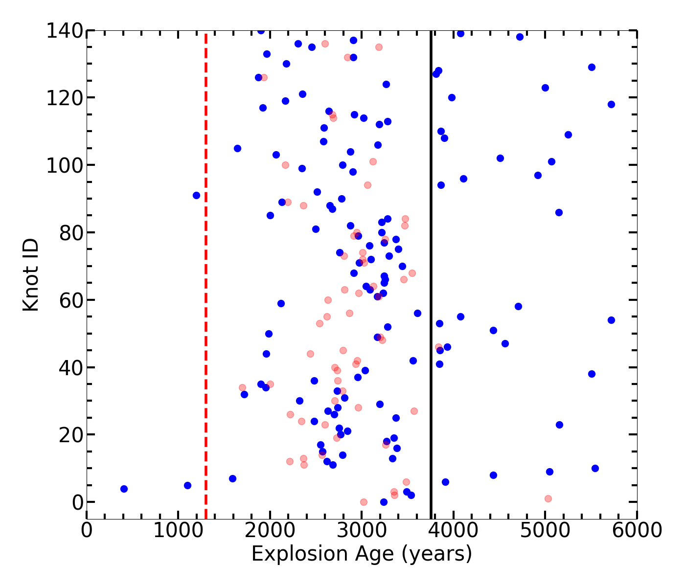
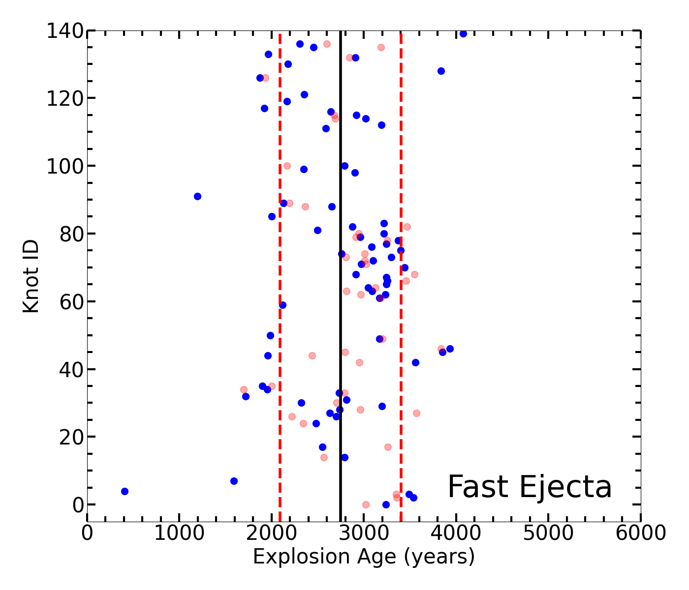
Figure A5: Similar to Figure 6 but using the proper motions from the automated procedure and including the results of only using the fastest ejecta. This results in an age of 3377 $\pm$ 2241 yr using all the knots and 2497 $\pm$ 638 yr using the fastest. The red shaded points correspond to the matching visually measured knots when applicable.

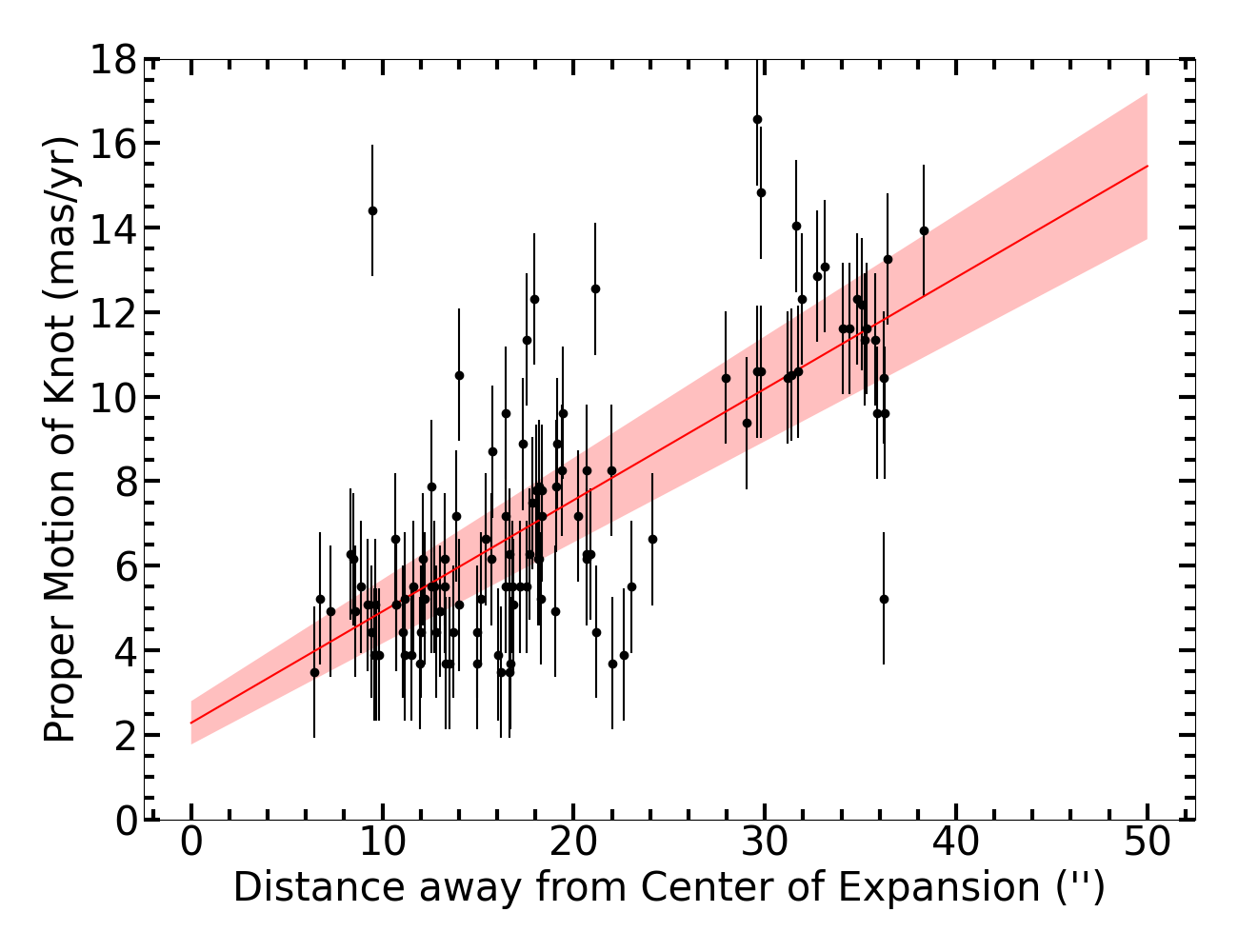
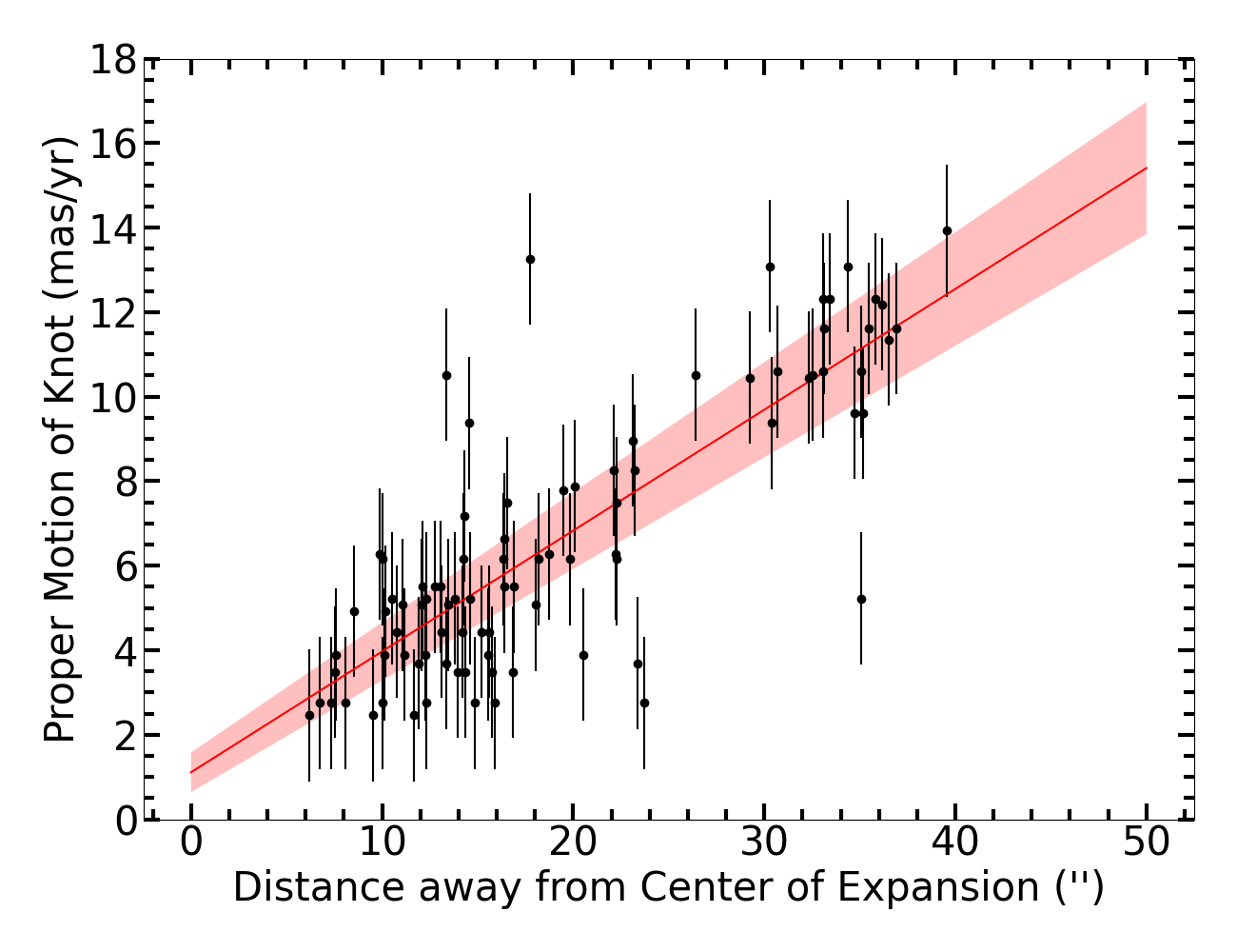
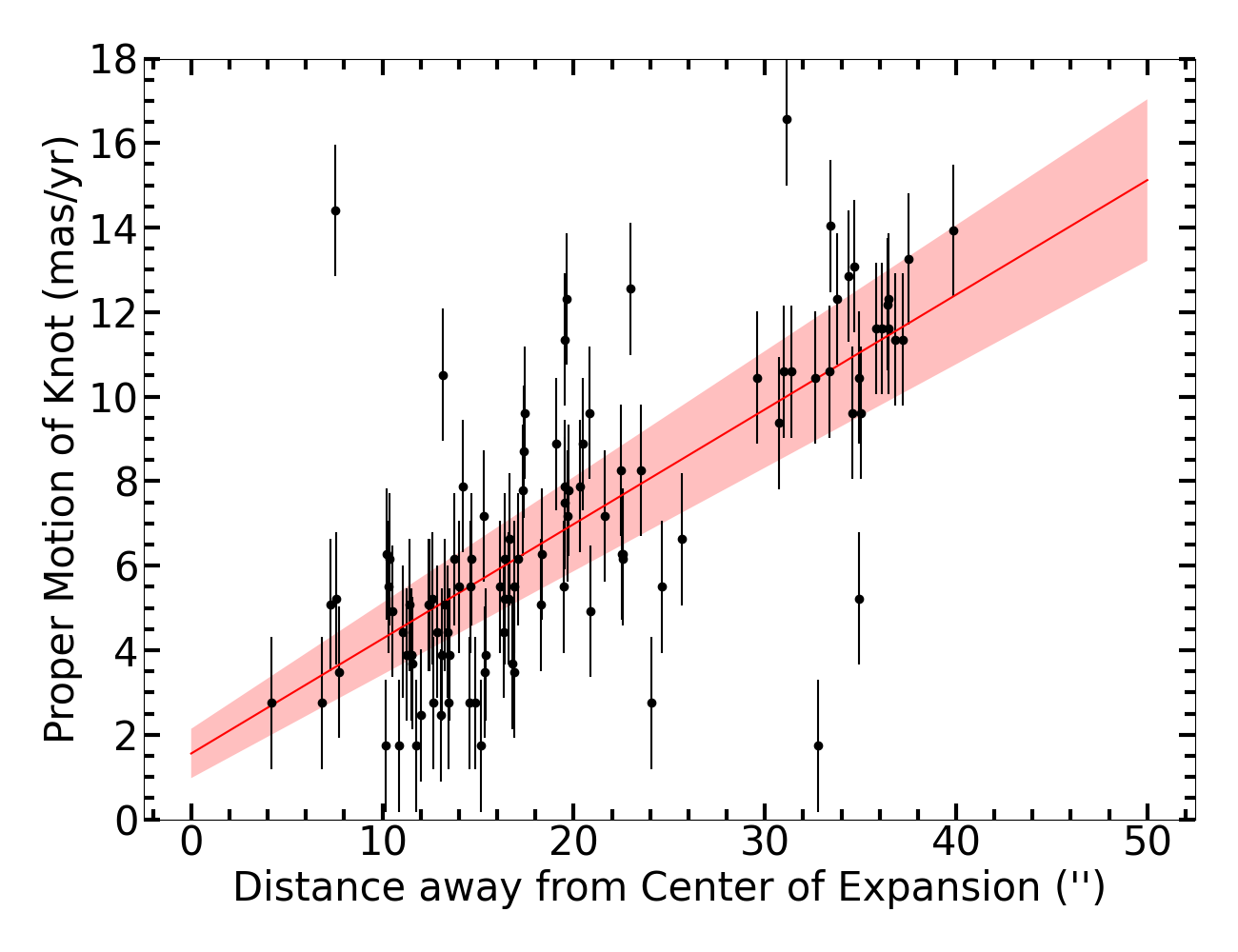
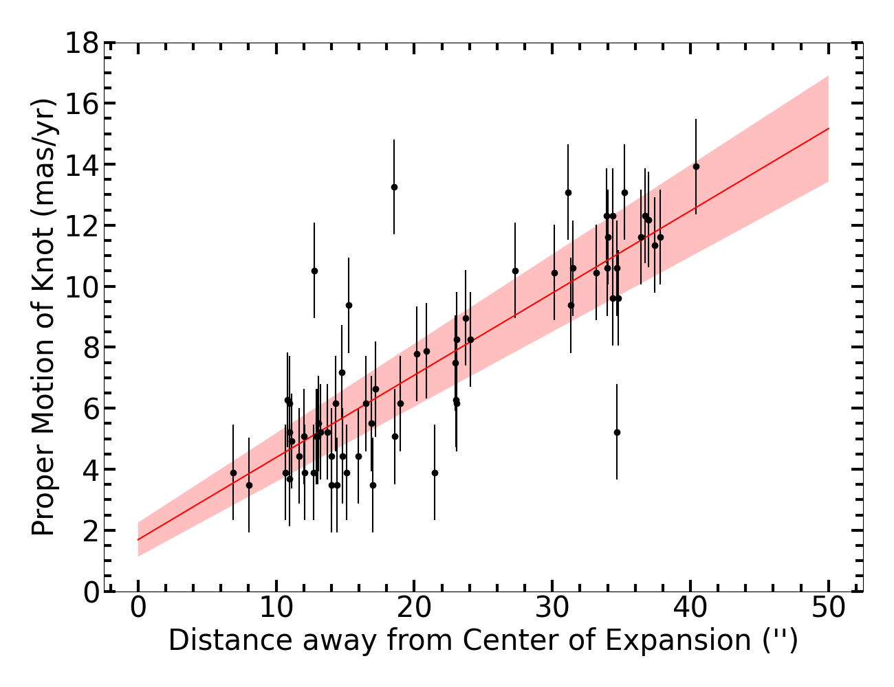
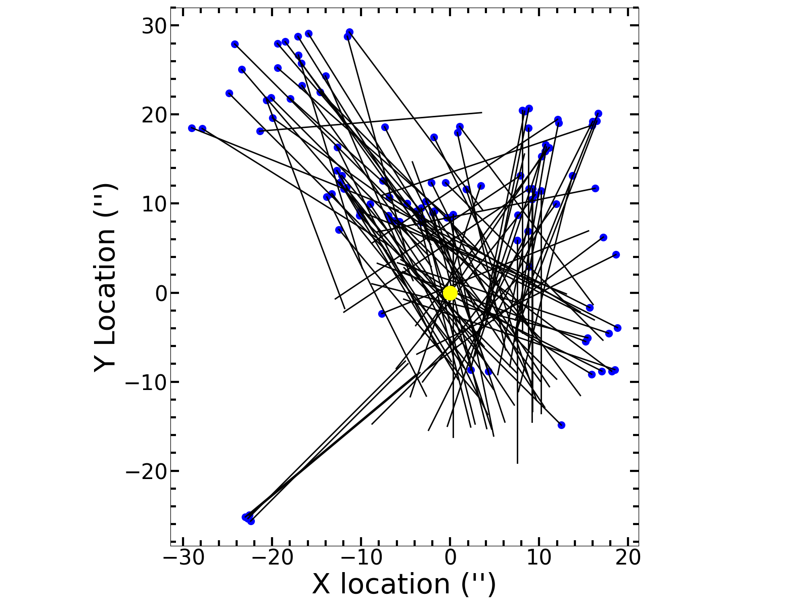
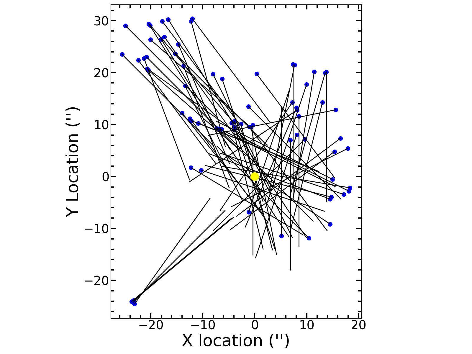
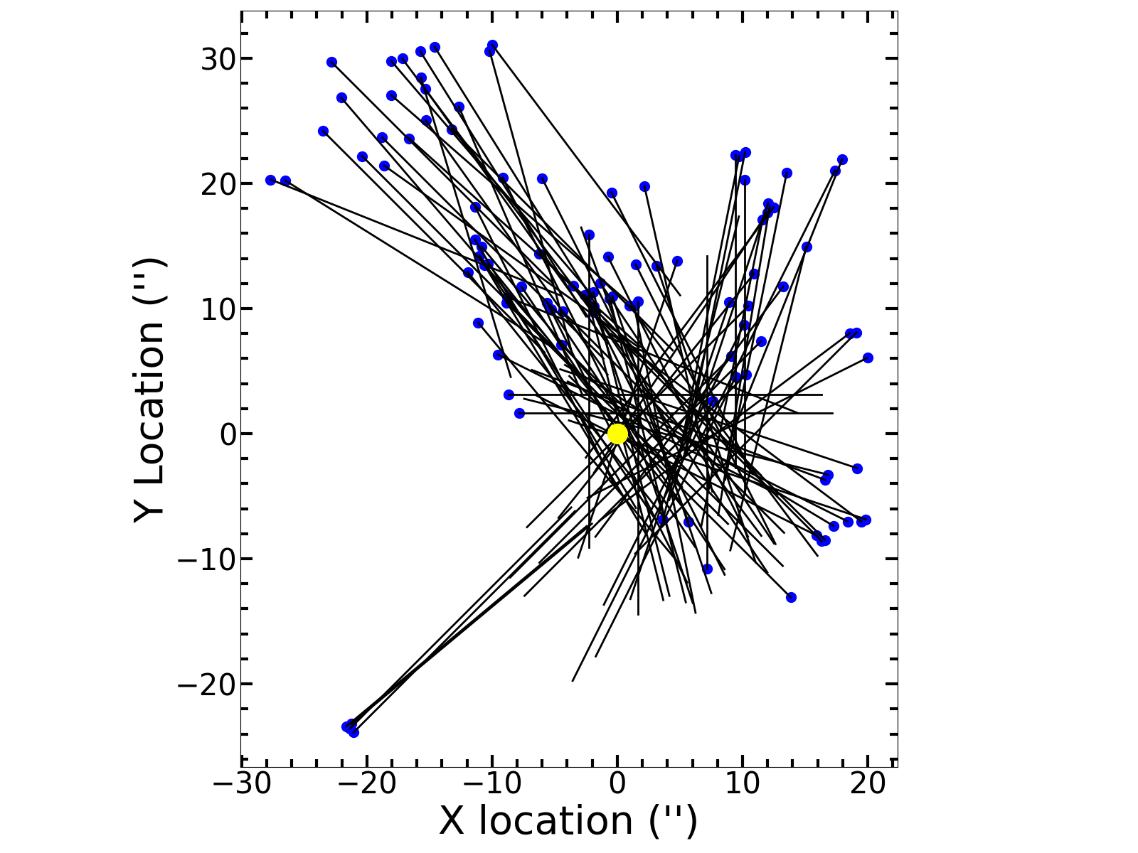
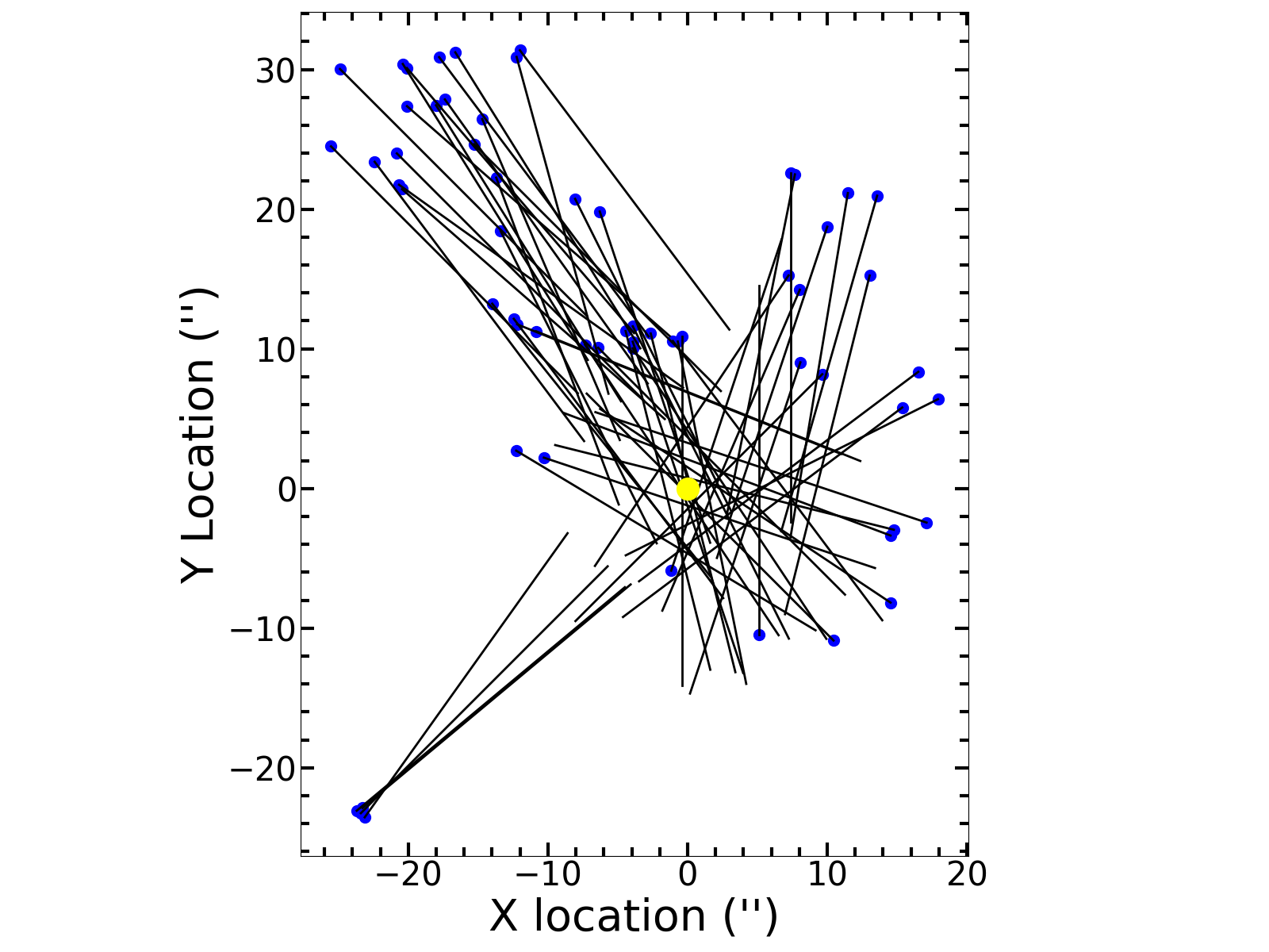
Figure A6: Similar to Figure A4 for the 3 mas yr^-1 lower limit (left), increase to 3-$\sigma$ of brightness (middle left), and reducing the trajectory and position angle difference of the knots to less than 45 degrees (middle right), and applying all three variations (right).

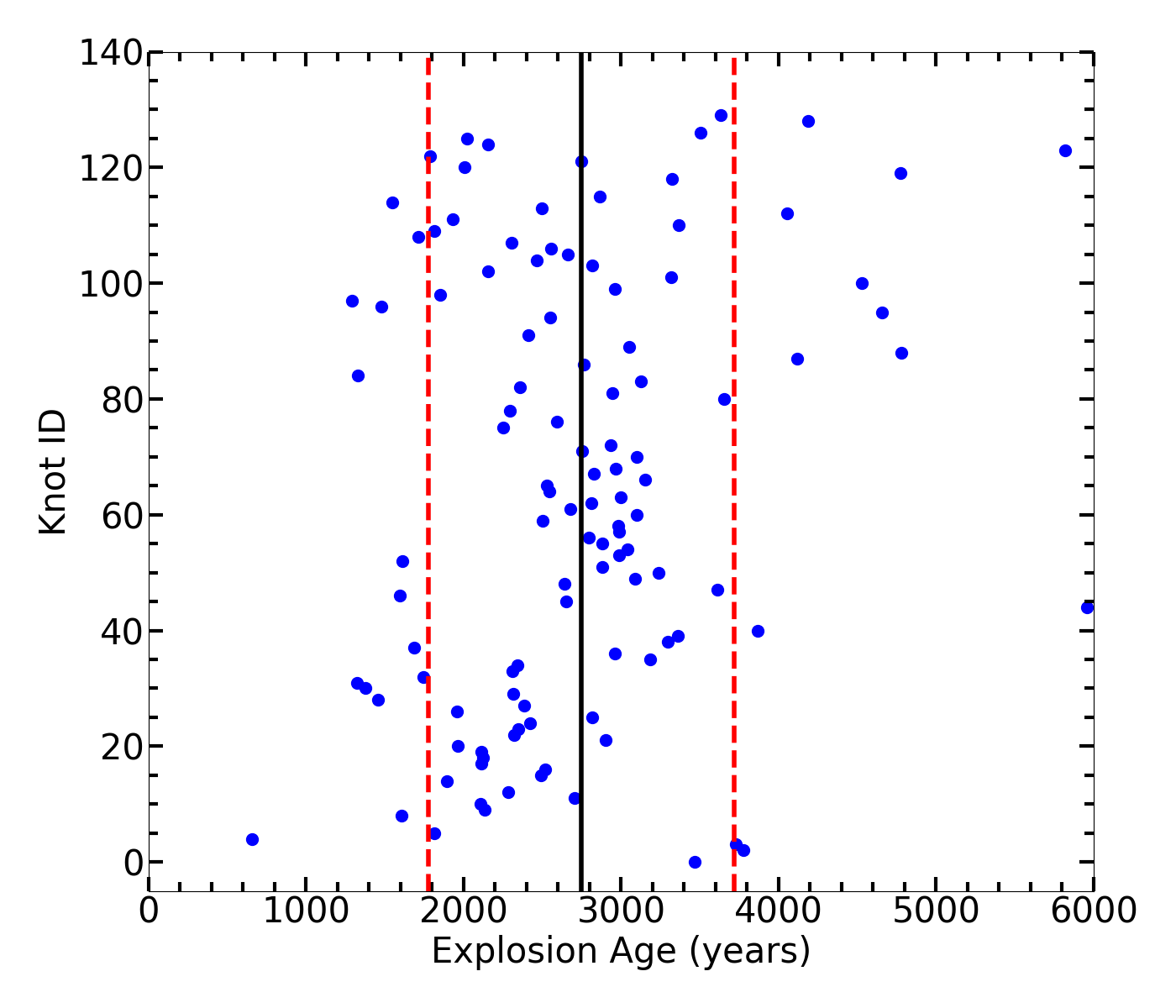
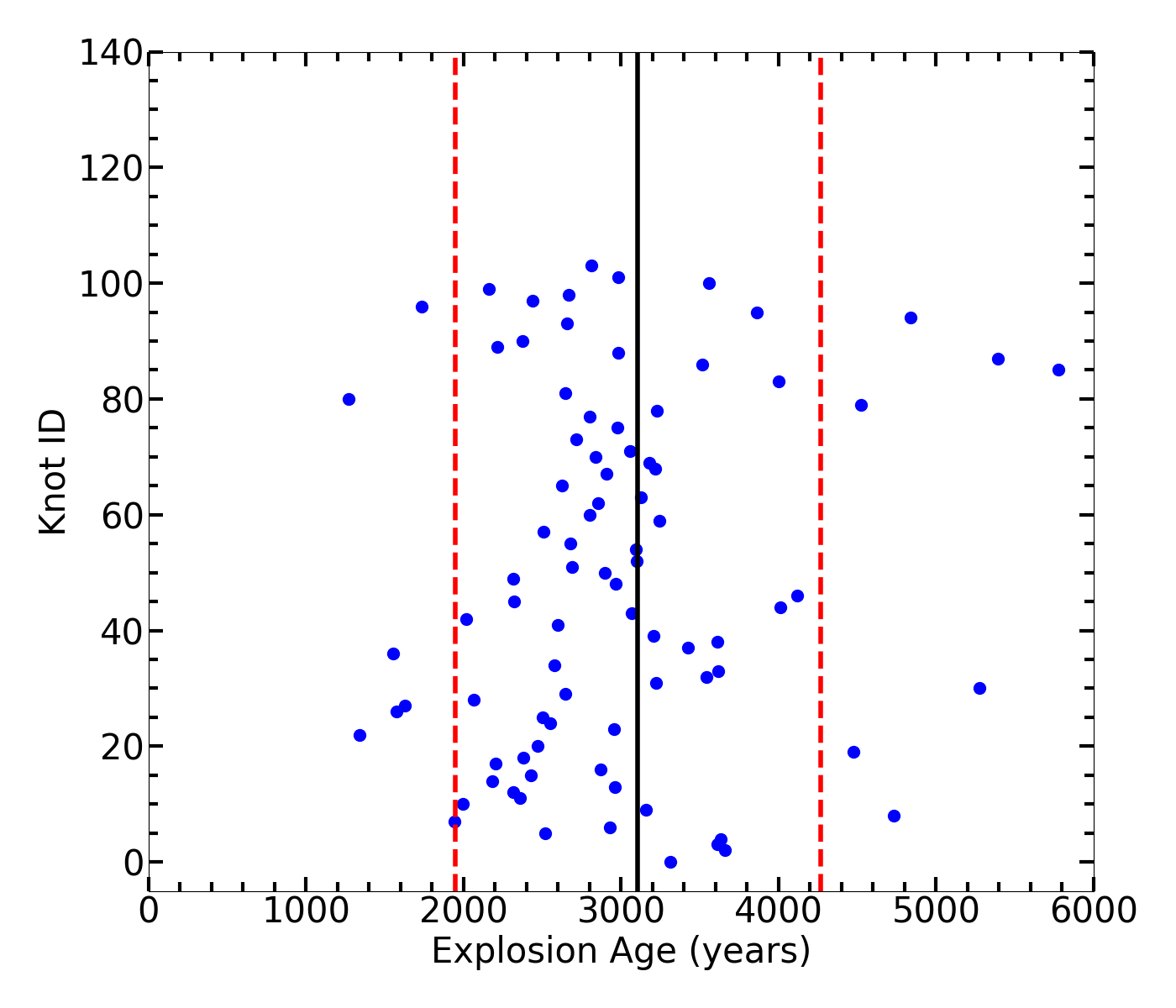
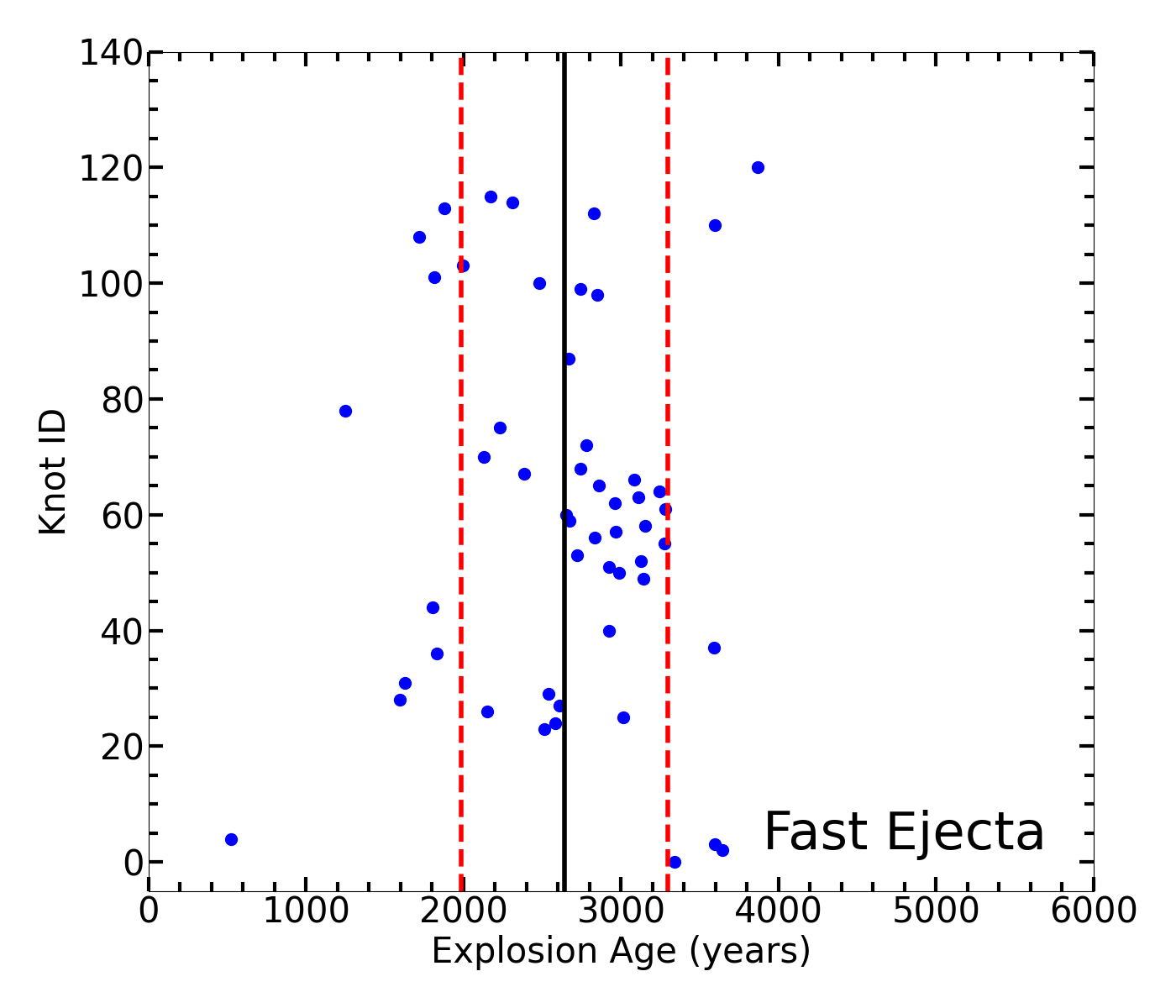
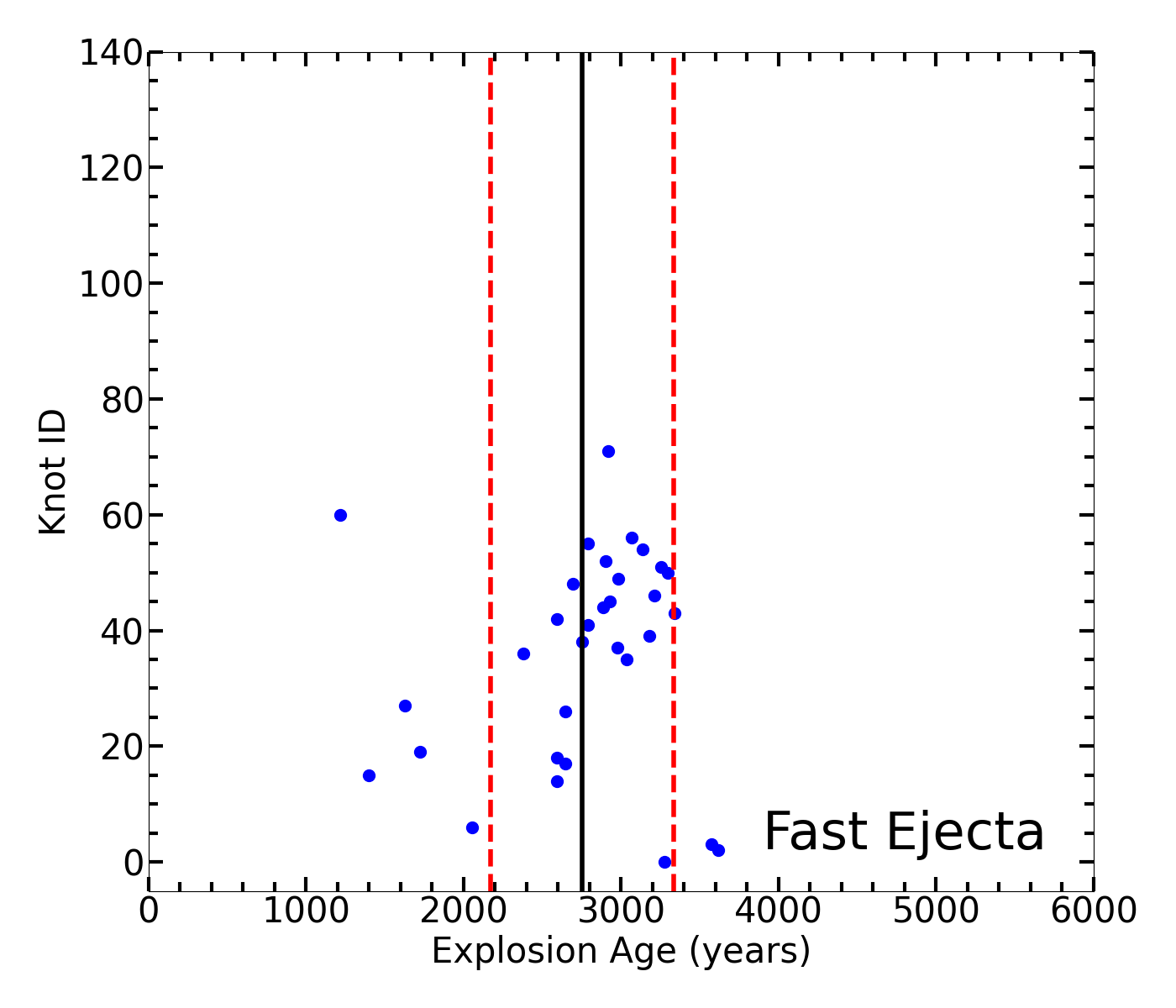
Figure A7: Similar to Figure 6 for the 3 mas yr^-1 lower limit (top left), increase to 3-$\sigma$ of brightness (top right),the trajectory and position angle difference of the knots to less than 45 degrees (bottom left), and using all the parameters (bottom right) that match closest to the visual inspection result.

Appendix B Additional Tables

Table A1: Anchor Star Coordinates

Star	RA (J2000)	Dec. (J2000)
1	5h24m53.7308s	69d38m15.310s
2	5h24m58.3686s	69d38m35.298s
3	5h24m57.8822s	69d38m46.447s
4	5h24m56.5386s	69d39m38.340s
5	5h24m58.2838s	69d39m39.118s
6	5h24m42.9113s	69d39m13.996s
7	5h24m47.0373s	69d38m43.292s
8	5h24m45.0608s	69d38m41.959s
9	5h24m49.4502s	69d38m29.224s
10	5h25m04.9414s	69d39m39.441s
11	5h25m00.6230s	69d38m00.893s
12	5h24m51.6282s	69d39m05.757s
13	5h24m49.5039s	69d38m47.073s
14	5h24m50.4438s	69d39m48.192s
15	5h24m52.2404s	69d39m22.696s
16	5h25m01.3169s	69d39m48.778s
17	5h24m44.4366s	69d39m09.882s
18	5h24m56.5344s	69d38m47.148s
19	5h25m04.2141s	69d40m09.653s
20	5h24m58.9991s	69d40m16.083s
21	5h25m07.3918s	69d40m02.308s
22	5h25m06.7103s	69d39m40.337s
23	5h25m11.2145s	69d38m20.227s
24	5h24m45.6713s	69d38m35.164s
25	5h24m47.2420s	69d38m17.491s
26	5h24m59.4994s	69d40m08.583s
27	5h25m08.2993s	69d39m18.289s
28	5h24m59.8352s	69d40m17.268s
29	5h24m49.7550s	69d38m06.447s
30	5h24m52.6476s	69d38m01.440s

Table A2: Manually Inspected Knot Measurements and Corresponding Automated Measurements

Knot	RA	Dec		Visual	Procedure		Automated	Procedure
			$\mu_{\alpha}$	$\sigma_{\mu_{\alpha}}$	$\mu_{\delta}$	$\sigma_{\mu_{\delta}}$	$\mu_{\alpha}$	$\mu_{\delta}$
	(J2000)	(J2000)	(mas yr-1)	(mas yr-1)	(mas yr-1)	(mas yr-1)	(mas yr-1)	(mas yr-1)
1	5h25m06.759s	69d39m04.815s	-8.095	0.452	-7.722	0.431	-7.386	-7.386
2	5h25m06.817s	69d39m04.523s	-5.075	0.472	-4.399	0.409	-3.693	-3.693
3	5h25m06.791s	69d39m04.138s	-7.498	0.469	-6.602	0.413	-7.386	-6.155
4	5h25m06.870s	69d39m04.341s	-7.866	0.487	-6.336	0.392	-7.386	-6.155
5	5h24m58.937s	69d38m48.660s	5.251	0.571	-2.335	0.254	NA	NA
6	5h24m59.498s	69d38m49.597s	2.766	0.412	-3.161	0.470	2.462	-3.693
7	5h24m59.334s	69d38m50.789s	3.786	0.403	-4.496	0.478	NA	NA
8	5h24m59.263s	69d38m49.396s	5.096	0.520	-3.409	0.347	NA	NA
9	5h24m59.365s	69d38m49.148s	5.557	0.543	-3.162	0.309	NA	NA
10	5h24m59.317s	69d38m49.096s	6.207	0.550	-3.349	0.297	NA	NA
11	5h24m59.068s	69d38m47.891s	5.977	0.555	-3.097	0.288	4.924	-3.693
12	5h24m58.914s	69d38m47.797s	7.006	0.578	-2.873	0.237	7.386	-2.462
13	5h24m59.357s	69d38m46.738s	6.259	0.589	-2.238	0.210	NA	NA
14	5h24m59.052s	69d38m43.732s	4.547	0.578	-1.877	0.238	3.693	-1.231
15	5h24m58.979s	69d38m35.721s	3.913	0.571	1.736	0.253	NA	NA
16	5h24m58.891s	69d38m34.856s	4.518	0.513	3.136	0.356	4.924	2.462
17	5h24m59.026s	69d38m35.230s	4.951	0.505	3.605	0.368	NA	NA
18	5h24m59.091s	69d38m33.413s	4.812	0.543	2.746	0.310	2.462	2.462
19	5h24m59.355s	69d38m35.500s	4.221	0.427	4.511	0.456	NA	NA
20	5h24m59.444s	69d38m35.482s	3.312	0.478	2.791	0.403	NA	NA
21	5h24m59.387s	69d38m35.145s	5.867	0.534	3.571	0.325	NA	NA
22	5h24m59.471s	69d38m35.149s	3.199	0.407	3.728	0.474	NA	NA
23	5h24m59.061s	69d38m32.842s	3.358	0.462	3.061	0.421	2.462	2.462
24	5h24m59.165s	69d38m32.899s	6.936	0.545	3.905	0.307	4.924	3.693
25	5h24m59.336s	69d38m33.396s	5.870	0.548	3.218	0.300	NA	NA
26	5h25m00.580s	69d38m33.323s	1.729	0.248	4.002	0.574	1.231	1.231
27	5h25m00.657s	69d38m33.912s	1.930	0.281	3.832	0.558	NA	NA
28	5h25m00.707s	69d38m35.283s	2.645	0.433	2.750	0.451	NA	NA
29	5h25m00.614s	69d38m30.296s	2.558	0.324	4.227	0.535	NA	NA
30	5h25m00.476s	69d38m33.102s	1.871	0.244	4.407	0.575	NA	NA
31	5h25m00.700s	69d38m28.663s	0.142	0.015	5.776	0.625	0.000	3.693
32	5h25m00.845s	69d38m27.202s	2.276	0.252	5.171	0.572	3.693	2.462
33	5h25m00.594s	69d38m26.570s	1.869	0.145	7.859	0.608	NA	NA
34	5h25m00.948s	69d38m26.000s	2.112	0.195	6.414	0.594	3.693 0	2.462
35	5h25m00.447s	69d38m23.793s	1.778	0.177	6.031	0.599	1.231	6.155
36	5h25m00.407s	69d38m22.524s	1.459	0.119	7.525	0.614	2.462	7.386
37	5h25m00.231s	69d38m22.238s	2.345	0.183	7.649	0.598	NA	NA
38	5h25m00.473s	69d38m23.509s	3.180	0.264	6.810	0.566	4.924	7.386
39	5h24m59.998s	69d38m22.286s	2.610	0.237	6.370	0.578	NA	NA
40	5h25m00.851s	69d38m18.795s	1.378	0.099	8.562	0.617	1.231	6.155
41	5h25m00.920s	69d38m18.666s	2.360	0.233	5.875	0.580	0.000	6.155
42	5h25m00.956s	69d38m17.995s	0.808	0.056	8.964	0.622	NA	NA
43	5h25m00.964s	69d38m18.212s	1.658	0.138	7.308	0.610	0.000	6.155
44	5h25m00.764s	69d38m18.370s	1.616	0.099	10.030	0.617	2.462	12.311
45	5h25m00.892s	69d38m18.986s	1.431	0.113	7.782	0.615	1.231	6.155
46	5h25m01.869s	69d38m20.792s	-1.263	0.074	10.628	0.621	NA	NA
47	5h25m02.200s	69d38m20.383s	-1.787	0.150	7.249	0.607	-3.693	4.924
48	5h25m02.373s	69d38m20.365s	-2.316	0.191	7.216	0.595	-3.693	4.924
49	5h25m02.258s	69d38m20.524s	-2.631	0.187	8.404	0.596	-3.693	4.924
50	5h25m02.309s	69d38m21.170s	-1.858	0.105	10.877	0.616	-2.462	11.080
51	5h25m02.559s	69d38m26.825s	-3.684	0.396	4.500	0.484	-3.693	3.693
52	5h25m02.397s	69d38m30.352s	-1.014	0.141	4.365	0.609	0.000	4.924
53	5h25m02.455s	69d38m30.719s	-1.352	0.141	5.836	0.609	-1.231	6.155
54	5h25m02.538s	69d38m30.703s	-4.625	0.405	5.428	0.476	-3.693	4.924
55	5h25m03.081s	69d38m30.761s	-2.899	0.377	3.830	0.498	-1.231	3.693
56	5h25m03.079s	69d38m29.633s	-2.074	0.300	3.791	0.548	-2.462	4.924
57	5h25m03.225s	69d38m29.853s	-4.040	0.461	3.700	0.422	-1.231	2.462
58	5h25m03.387s	69d38m28.857s	-2.748	0.259	6.035	0.569	-3.693	4.924
59	5h25m03.553s	69d38m31.191s	-4.421	0.466	3.954	0.417	-3.693	3.693
60	5h25m03.644s	69d38m31.047s	-4.108	0.393	5.077	0.486	-4.924	2.462
61	5h25m03.738s	69d38m30.971s	-4.446	0.443	4.420	0.441	-2.462	3.693
62	5h25m03.792s	69d38m30.488s	-3.843	0.400	4.604	0.480	-2.462	4.924
63	5h25m04.737s	69d38m37.017s	-4.387	0.599	1.320	0.180	NA	NA
64	5h25m04.584s	69d38m38.620s	-7.044	0.540	4.111	0.315	NA	NA
65	5h25m04.800s	69d38m36.432s	-6.623	0.483	5.433	0.396	NA	NA
66	5h25m03.965s	69d38m41.964s	-2.947	0.602	0.823	0.168	-2.462	1.231
67	5h25m04.343s	69d38m40.948s	-4.563	0.553	2.407	0.292	NA	NA
68	5h25m03.941s	69d38m42.226s	-5.002	0.622	0.481	0.060	-2.462	1.231
69	5h25m04.387s	69d38m30.020s	-5.281	0.410	6.064	0.471	-6.155	2.462
70	5h25m04.664s	69d38m29.489s	-5.792	0.441	5.809	0.443	NA	NA
71	5h25m04.712s	69d38m29.118s	-5.238	0.465	4.714	0.418	NA	NA
72	5h25m05.020s	69d38m28.243s	-5.438	0.469	4.799	0.414	-4.924	6.155
73	5h25m05.009s	69d38m28.027s	-4.951	0.417	5.517	0.465	-4.924	6.155
74	5h25m04.751s	69d38m27.468s	-4.284	0.342	6.548	0.523	-3.693	6.155
75	5h25m05.117s	69d38m28.383s	-3.508	0.360	4.986	0.511	-3.693	7.386
76	5h25m04.831s	69d38m26.683s	-4.528	0.413	5.136	0.469	-4.924	7.386
77	5h25m04.797s	69d38m26.002s	-5.496	0.402	6.537	0.478	-6.155	7.386
78	5h25m02.870s	69d38m21.258s	-3.230	0.273	6.654	0.562	-2.462	4.924
79	5h25m02.811s	69d38m21.684s	-5.987	0.404	7.064	0.477	-2.462	4.924
80	5h25m03.575s	69d38m22.023s	-3.531	0.270	7.370	0.564	0.000	1.231
81	5h25m03.874s	69d38m20.501s	-3.165	0.291	6.015	0.553	-3.693	7.386
82	5h25m03.436s	69d38m23.201s	-2.373	0.198	7.098	0.593	NA	NA
83	5h25m04.893s	69d38m22.848s	-4.533	0.306	8.081	0.545	-3.693	7.386
84	5h25m04.797s	69d38m21.717s	-7.334	0.410	8.452	0.472	NA	NA
85	5h25m04.663s	69d38m20.967s	-7.508	0.428	7.979	0.455	NA	NA
86	5h25m04.954s	69d38m18.989s	-5.288	0.281	10.497	0.558	NA	NA
87	5h25m05.116s	69d38m18.782s	-6.096	0.363	8.557	0.509	NA	NA
88	5h25m05.411s	69d38m19.262s	-7.661	0.502	5.670	0.372	NA	NA
89	5h25m08.036s	69d38m20.676s	-11.101	0.512	7.791	0.359	-12.311	4.924
90	5h25m07.979s	69d38m20.386s	-10.437	0.505	7.603	0.368	-12.311	4.924
91	5h25m07.921s	69d38m20.738s	-8.091	0.394	9.951	0.485	-9.848	6.155
92	5h25m07.220s	69d38m16.762s	-9.750	0.454	9.215	0.429	-8.617	8.617
93	5h25m07.046s	69d38m17.499s	-10.700	0.463	9.720	0.420	NA	NA
94	5h25m06.250s	69d38m19.801s	-8.183	0.501	6.116	0.374	-8.617	6.155
95	5h25m06.290s	69d38m19.507s	-8.475	0.492	6.644	0.386	-8.617	6.155
96	5h25m06.317s	69d38m17.245s	-6.808	0.433	7.101	0.451	-7.386	7.386
97	5h25m05.259s	69d38m16.604s	-6.608	0.401	7.889	0.479	-7.386	7.386
98	5h25m05.423s	69d38m15.945s	-5.608	0.298	10.350	0.550	NA	NA
99	5h25m05.352s	69d38m15.983s	-6.149	0.357	8.852	0.513	NA	NA
100	5h25m05.648s	69d38m15.853s	-6.412	0.367	8.849	0.506	-6.155	8.617
101	5h25m05.767s	69d38m16.143s	-6.894	0.343	10.506	0.523	-6.155	8.617
102	5h25m05.794s	69d38m15.290s	-6.897	0.366	9.563	0.507	NA	NA
103	5h25m06.181s	69d38m13.869s	-7.882	0.410	9.053	0.471	-9.848	8.617
104	5h25m05.608s	69d38m13.780s	-6.183	0.314	10.619	0.540	-6.155	8.617
105	5h25m06.015s	69d38m13.013s	-8.498	0.391	10.610	0.488	NA	NA
106	5h25m05.661s	69d38m13.407s	-6.182	0.323	10.241	0.535	-6.155	8.617
107	5h25m05.593s	69d38m12.558s	-6.322	0.313	10.925	0.541	NA	NA
108	5h25m07.099s	69d38m11.216s	-9.856	0.435	10.153	0.448	-9.848	9.848
109	5h25m06.241s	69d38m10.852s	-7.146	0.375	9.535	0.500	-7.386	8.617
110	5h25m05.609s	69d38m10.424s	-7.850	0.387	9.943	0.491	-6.155	9.848
111	5h25m05.343s	69d38m08.948s	-5.298	0.301	9.658	0.548	NA	NA
112	5h25m05.381s	69d38m11.992s	-6.841	0.346	10.297	0.521	NA	NA
113	5h25m05.438s	69d38m10.191s	-7.160	0.344	10.850	0.522	-6.155	9.848
114	5h25m04.640s	69d38m10.040s	-3.924	0.241	9.388	0.577	-7.386	9.848
115	5h25m04.454s	69d38m09.844s	-4.261	0.246	9.951	0.575	NA	NA
116	5h24m58.646s	69d38m25.981s	6.982	0.425	7.526	0.458	NA	NA
117	5h25m01.395s	69d38m49.800s	1.921	0.302	-3.487	0.547	NA	NA
118	5h25m01.442s	69d38m50.223s	0.035	0.005	-4.109	0.625	NA	NA
119	5h24m59.732s	69d38m20.293s	3.725	0.301	6.767	0.548	0.000	3.693
120	5h25m05.432s	69d38m08.588s	-6.583	0.334	10.405	0.528	NA	NA

Note. — Positive values indicate direction to the north and east for RA and Dec. respectively. Results of the automated procedure are matched when applicable.

References

- Ackermann et al. (2016) Ackermann, M., Albert, A., Atwood, W. B., et al. 2016, A&A, 586, A71, doi: 10.1051/0004-6361/201526920
- Astropy Collaboration et al. (2013) Astropy Collaboration, Robitaille, T. P., Tollerud, E. J., et al. 2013, A&A, 558, A33, doi: 10.1051/0004-6361/201322068
- Astropy Collaboration et al. (2018) Astropy Collaboration, Price-Whelan, A. M., Sipőcz, B. M., et al. 2018, AJ, 156, 123, doi: 10.3847/1538-3881/aabc4f
- Bally et al. (2002) Bally, J., Reipurth, B., Walawender, J., & Armond, T. 2002, AJ, 124, 2152, doi: 10.1086/342850
- Bamba et al. (2018) Bamba, A., Ohira, Y., Yamazaki, R., et al. 2018, ApJ, 854, 71, doi: 10.3847/1538-4357/aaa5a0
- Banas et al. (1997) Banas, K. R., Hughes, J. P., Bronfman, L., & Nyman, L. Å. 1997, ApJ, 480, 607, doi: 10.1086/303989
- Banovetz et al. (2021) Banovetz, J., Milisavljevic, D., Sravan, N., et al. 2021, ApJ, 912, 33, doi: 10.3847/1538-4357/abe2a7
- Bhalerao et al. (2019) Bhalerao, J., Park, S., Schenck, A., Post, S., & Hughes, J. P. 2019, ApJ, 872, 31, doi: 10.3847/1538-4357/aafafd
- Blair et al. (2000) Blair, W. P., Morse, J. A., & Raymond et al., J. C. 2000, ApJ, 537, 667, doi: 10.1086/309077
- Borkowski et al. (2007) Borkowski, K. J., Hendrick, S. P., & Reynolds, S. P. 2007, ApJ, 671, L45, doi: 10.1086/524733
- Borkowski et al. (2020) Borkowski, K. J., Miltich, W., & Reynolds, S. P. 2020, ApJ, 905, L19, doi: 10.3847/2041-8213/abcda7
- Burrows et al. (2019) Burrows, A., Radice, D., & Vartanyan, D. 2019, MNRAS, 485, 3153, doi: 10.1093/mnras/stz543
- Chen et al. (2003) Chen, Y., Zhang, F., Williams, R. M., & Wang, Q. D. 2003, ApJ, 595, 227, doi: 10.1086/377353
- Chevalier (2005) Chevalier, R. A. 2005, ApJ, 619, 839, doi: 10.1086/426584
- Clark (1982) Clark, D. H. 1982, The Observatory, 102, 111
- Currie et al. (1996) Currie, D. G., Dowling, D. M., & Shaya et al., E. J. 1996, AJ, 112, 1115, doi: 10.1086/118083
- Danziger & Dennefeld (1976) Danziger, I. J., & Dennefeld, M. 1976, ApJ, 207, 394, doi: 10.1086/154507
- Dickel & Milne (1995) Dickel, J. R., & Milne, D. K. 1995, AJ, 109, 200, doi: 10.1086/117266
- Dopita et al. (2018) Dopita, M. A., Vogt, F. P. A., Sutherland, R. S., et al. 2018, ApJS, 237, 10, doi: 10.3847/1538-4365/aac837
- Favata et al. (1997) Favata, F., Vink, J., Parmar, A. N., Kaastra, J. S., & Mineo, T. 1997, A&A, 324, L45. https://arxiv.org/abs/astro-ph/9707055
- Ferrand et al. (2021) Ferrand, G., Warren, D. C., Ono, M., et al. 2021, ApJ, 906, 93, doi: 10.3847/1538-4357/abc951
- Fesen (2001) Fesen, R. A. 2001, ApJS, 133, 161, doi: 10.1086/319181
- Fesen & Gunderson (1996) Fesen, R. A., & Gunderson, K. S. 1996, ApJ, 470, 967, doi: 10.1086/177923
- Fesen et al. (2006) Fesen, R. A., Hammell, M. C., & Morse et al., J. 2006, ApJ, 645, 283, doi: 10.1086/504254
- Fesen & Milisavljevic (2016) Fesen, R. A., & Milisavljevic, D. 2016, ApJ, 818, 17, doi: 10.3847/0004-637X/818/1/17
- Fesen et al. (2011) Fesen, R. A., Zastrow, J. A., Hammell, M. C., Shull, J. M., & Silvia, D. W. 2011, ApJ, 736, 109, doi: 10.1088/0004-637X/736/2/109
- Finkelstein et al. (2006) Finkelstein, S. L., Morse, J. A., Green, J. C., et al. 2006, ApJ, 641, 919, doi: 10.1086/500570
- Fox et al. (2022) Fox, O. D., Van Dyk, S. D., Williams, B. F., et al. 2022, ApJ, 929, L15, doi: 10.3847/2041-8213/ac5890
- Gaensler & Wallace (2003) Gaensler, B. M., & Wallace, B. J. 2003, ApJ, 594, 326, doi: 10.1086/376861
- Ghavamian et al. (2005) Ghavamian, P., Hughes, J. P., & Williams, T. B. 2005, ApJ, 635, 365, doi: 10.1086/497283
- Gonzaga et al. (2012) Gonzaga, S., Hack, W., Fruchter, A., & Mack, J. 2012, The DrizzlePac Handbook
- Graczyk et al. (2014) Graczyk, D., Pietrzyński, G., Thompson, I. B., et al. 2014, ApJ, 780, 59, doi: 10.1088/0004-637X/780/1/59
- Green (2012) Green, W. 2012, Society for Astronomical Sciences Annual Symposium, 31, 159
- H. E. S. S. Collaboration et al. (2015) H. E. S. S. Collaboration, Abramowski, A., Aharonian, F., et al. 2015, Science, 347, 406, doi: 10.1126/science.1261313
- Hammell & Fesen (2008) Hammell, M. C., & Fesen, R. A. 2008, ApJS, 179, 195, doi: 10.1086/591528
- Hartigan et al. (2001) Hartigan, P., Morse, J. A., Reipurth, B., Heathcote, S., & Bally, J. 2001, ApJ, 559, L157, doi: 10.1086/323976
- Holland-Ashford et al. (2017) Holland-Ashford, T., Lopez, L. A., Auchettl, K., Temim, T., & Ramirez-Ruiz, E. 2017, ApJ, 844, 84, doi: 10.3847/1538-4357/aa7a5c
- Hughes (1987) Hughes, J. P. 1987, ApJ, 314, 103, doi: 10.1086/165043
- Janka et al. (2016) Janka, H.-T., Melson, T., & Summa, A. 2016, Annual Review of Nuclear and Particle Science, 66, 341, doi: 10.1146/annurev-nucl-102115-044747
- Kamper & van den Bergh (1976) Kamper, K., & van den Bergh, S. 1976, ApJS, 32, 351, doi: 10.1086/190400
- Katsuda et al. (2018) Katsuda, S., Morii, M., & Janka et al., H.-T. 2018, ApJ, 856, 18, doi: 10.3847/1538-4357/aab092
- Kerzendorf et al. (2019) Kerzendorf, W. E., Do, T., de Mink, S. E., et al. 2019, A&A, 623, A34, doi: 10.1051/0004-6361/201732206
- Kiminki et al. (2016) Kiminki, M. M., Reiter, M., & Smith, N. 2016, MNRAS, 463, 845, doi: 10.1093/mnras/stw2019
- Lang et al. (2010) Lang, D., Hogg, D. W., Mierle, K., Blanton, M., & Roweis, S. 2010, AJ, 139, 1782, doi: 10.1088/0004-6256/139/5/1782
- Lasker (1980) Lasker, B. M. 1980, ApJ, 237, 765, doi: 10.1086/157923
- Law et al. (2020) Law, C. J., Milisavljevic, D., Patnaude, D. J., et al. 2020, ApJ, 894, 73, doi: 10.3847/1538-4357/ab873a
- Lee et al. (2014) Lee, J.-J., Park, S., Hughes, J. P., & Slane, P. O. 2014, ApJ, 789, 7, doi: 10.1088/0004-637X/789/1/7
- Li et al. (2021) Li, C.-J., Seitenzahl, I. R., Ishioka, R., et al. 2021, ApJ, 915, 20, doi: 10.3847/1538-4357/abf7c5
- Long et al. (2022) Long, X., Patnaude, D. J., Plucinsky, P. P., & Gaetz, T. J. 2022, ApJ, 932, 117, doi: 10.3847/1538-4357/ac704b
- Lopez & Fesen (2018) Lopez, L. A., & Fesen, R. A. 2018, SSR, 214, 44, doi: 10.1007/s11214-018-0481-x
- Milisavljevic & Fesen (2013) Milisavljevic, D., & Fesen, R. A. 2013, ApJ, 772, 134, doi: 10.1088/0004-637X/772/2/134
- Milisavljevic & Fesen (2017) —. 2017, in Handbook of Supernovae, ed. A. W. Alsabti & P. Murdin (Springer International Publishing AG), 2211, doi: 10.1007/978-3-319-21846-5_97
- Milisavljevic et al. (2010) Milisavljevic, D., Fesen, R. A., Gerardy, C. L., Kirshner, R. P., & Challis, P. 2010, ApJ, 709, 1343, doi: 10.1088/0004-637X/709/2/1343
- Morse et al. (2001) Morse, J. A., Kellogg, J. R., Bally, J., et al. 2001, ApJ, 548, L207, doi: 10.1086/319092
- Morse et al. (1995) Morse, J. A., Winkler, P. F., & Kirshner, R. P. 1995, AJ, 109, 2104, doi: 10.1086/117436
- Murdin & Clark (1979) Murdin, P., & Clark, D. H. 1979, MNRAS, 189, 501, doi: 10.1093/mnras/189.3.501
- Orlando et al. (2021) Orlando, S., Wongwathanarat, A., Janka, H. T., et al. 2021, A&A, 645, A66, doi: 10.1051/0004-6361/202039335
- Orlando et al. (2022) —. 2022, arXiv e-prints, arXiv:2202.01643. https://arxiv.org/abs/2202.01643
- Panagia et al. (1991) Panagia, N., Gilmozzi, R., Macchetto, F., Adorf, H. M., & Kirshner, R. P. 1991, ApJ, 380, L23, doi: 10.1086/186164
- Park et al. (2007) Park, S., Hughes, J. P., Slane, P. O., et al. 2007, ApJ, 670, L121, doi: 10.1086/524406
- Patnaude & Fesen (2014) Patnaude, D. J., & Fesen, R. A. 2014, ApJ, 789, 138, doi: 10.1088/0004-637X/789/2/138
- Reed et al. (1995) Reed, J. E., Hester, J. J., Fabian, A. C., & Winkler, P. F. 1995, ApJ, 440, 706, doi: 10.1086/175308
- Sano et al. (2020) Sano, H., Plucinsky, P. P., Bamba, A., et al. 2020, ApJ, 902, 53, doi: 10.3847/1538-4357/abb469
- Sasaki et al. (2006) Sasaki, M., Gaetz, T. J., Blair, W. P., et al. 2006, ApJ, 642, 260, doi: 10.1086/500789
- Scowcroft et al. (2016) Scowcroft, V., Freedman, W. L., Madore, B. F., et al. 2016, ApJ, 816, 49, doi: 10.3847/0004-637X/816/2/49
- Sharda et al. (2020) Sharda, P., Gaetz, T. J., Kashyap, V. L., & Plucinsky, P. P. 2020, ApJ, 894, 145, doi: 10.3847/1538-4357/ab8a46
- Silverman (1982) Silverman, B. W. 1982, Applied Statistics, 31, 67
- Smartt (2009) Smartt, S. J. 2009, ARA&A, 47, 63, doi: 10.1146/annurev-astro-082708-101737
- Smithsonian Astrophysical Observatory (2000) Smithsonian Astrophysical Observatory. 2000, SAOImage DS9: A utility for displaying astronomical images in the X11 window environment. http://ascl.net/0003.002
- Sutherland & Dopita (1995) Sutherland, R. S., & Dopita, M. A. 1995, ApJ, 439, 365, doi: 10.1086/175180
- Temim et al. (2022) Temim, T., Slane, P., Raymond, J. C., et al. 2022, arXiv e-prints, arXiv:2205.01798. https://arxiv.org/abs/2205.01798
- Thorstensen et al. (2001) Thorstensen, J. R., Fesen, R. A., & van den Bergh, S. 2001, AJ, 122, 297, doi: 10.1086/321138
- Vink et al. (2022) Vink, J., Patnaud, D. J., & Castro, D. 2022, arXiv e-prints, arXiv:2201.08911. https://arxiv.org/abs/2201.08911
- Vogt & Dopita (2011) Vogt, F., & Dopita, M. A. 2011, AP&SS, 331, 521, doi: 10.1007/s10509-010-0479-7
- Vogt et al. (2018) Vogt, F. P. A., Bartlett, E. S., Seitenzahl, I. R., et al. 2018, Nature Astronomy, 2, 465, doi: 10.1038/s41550-018-0433-0
- Vogt et al. (2017) Vogt, F. P. A., Seitenzahl, I. R., Dopita, M. A., & Ghavamian, P. 2017, A&A, 602, L4, doi: 10.1051/0004-6361/201730756
- Weil et al. (2020) Weil, K. E., Fesen, R. A., Patnaude, D. J., et al. 2020, ApJ, 891, 116, doi: 10.3847/1538-4357/ab76bf
- Westerlund & Mathewson (1966) Westerlund, B. E., & Mathewson, D. S. 1966, MNRAS, 131, 371, doi: 10.1093/mnras/131.3.371
- Williams et al. (2006) Williams, B. J., Borkowski, K. J., Reynolds, S. P., et al. 2006, ApJ, 652, L33, doi: 10.1086/509876
- Winkler et al. (2010) Winkler, P. F., Garber, J. H., Plunkett, A. L. D., Twelker, K., & Long, K. S. 2010, in AAS/High Energy Astrophysics Division, Vol. 11, AAS/High Energy Astrophysics Division #11, 18.13
- Winkler et al. (2009) Winkler, P. F., Twelker, K., & Reith et al., C. N. 2009, ApJ, 692, 1489, doi: 10.1088/0004-637X/692/2/1489
- Wongwathanarat et al. (2015) Wongwathanarat, A., Müller, E., & Janka, H. T. 2015, A&A, 577, A48, doi: 10.1051/0004-6361/201425025
- Xi et al. (2019) Xi, L., Gaetz, T. J., Plucinsky, P. P., Hughes, J. P., & Patnaude, D. J. 2019, ApJ, 874, 14, doi: 10.3847/1538-4357/ab09ea