CRADL: Contrastive Representations for Unsupervised Anomaly Detection and Localization

Abstract

Unsupervised anomaly detection in medical imaging aims to detect and localize arbitrary anomalies without requiring annotated anomalous data during training. Often, this is achieved by learning a data distribution of normal samples and detecting anomalies as regions in the image which deviate from this distribution. Most current state-of-the-art methods use latent variable generative models operating directly on the images. However, generative models have been shown to mostly capture low-level features, s.a. pixel-intensities, instead of rich semantic features, which also applies to their representations. We circumvent this problem by proposing CRADL whose core idea is to model the distribution of normal samples directly in the low-dimensional representation space of an encoder trained with a contrastive pretext-task. By utilizing the representations of contrastive learning, we aim to fix the over-fixation on low-level features and learn more semantic-rich representations. Our experiments on anomaly detection and localization tasks using three distinct evaluation datasets show that 1) contrastive representations are superior to representations of generative latent variable models and 2) the CRADL framework shows competitive or superior performance to state-of-the-art.

1 Introduction

The task of anomaly detection is a long-standing task in the medical domain, with many diseases being defined by their deviation from what is considered to be normal [1]. In medical image analysis detecting and localizing anomalies is, therefore also often the general goal. With powerful deep learning algorithms, this task is often tackled using supervised machine learning, which can be highly effective given that enough diseased cases are available and annotated during the training process [2, 3]. However, most supervised models are not explicitly designed to handle Out-of-Distribution (OoD) data. They thus might struggle to extrapolate to new settings e.g., the heterogeneity of diseases beyond the training distribution [4]. Consequently, each new class of pathology or imaging modality necessitates the creation of new annotated datasets—a process that scales poorly with the large number of existing pathologies and the ever-increasing amount of image acquisition methods. Unsupervised anomaly detection promises to deliver predictions in the absence of annotated diseased data. Thus, overcoming the need for cumbersome manual annotations of diseased images, this class of methods could offer a far greater breadth of applications. In principle, this can be realized by learning the distribution of healthy samples. Images (or rather some voxels in the images) ‘deviating’ from this distribution are then defined as outliers. The problem of detecting these deviations can be posed as an OoD detection problem similar to the statistical tests underlying blood tests using reference ranges [5]. Specifically, in the medical imaging domain, the current state-of-the-art methods for anomaly detection are latent variable generative models operating directly on image space, mainly different subtypes of and scoring methods based on Variational Autoencoders (VAEs) and Generative Adversarial Networks (GANs) [6, 7, 8]. It has been shown, however, that the likelihoods of generative models tend to focus on low-level features such as background characteristics [9, 10, 11, 12] and that their representations have problems capturing semantic information [9, 13]. Therefore the anomaly scores of these methods built on their likelihoods and representations are heavily dependent on the aforementioned characteristics not capturing fine semantic information.

Driven by the hypothesis that more discriminative semantic features are superior to low-level features, we investigate if the representations obtained with self-supervised contrastive learning can aid unsupervised anomaly detection and localization.

For this, we propose CRADL, a simple unsupervised representation-based OoD framework consisting of a generative model working on the representations of a feature extractor, trained in a self-supervised fashion based on SimCLR [14].

Our experimental results comparing it with state-of-the-art latent generative models and using the representation-based approach with generative representations on MRI-Brain lead to the following findings:

• In the low-dimensional representation space of CRADL (and generative models) computationally inexpensive generative models allow for reliable detection and even localization of anomalies.

• CRADL is comparable with state-of-the-art anomaly detection and localization approaches and is better suited to detect fine deviations from normality.

• Representations obtained with the contrastive pretext task of CRADL outperform representations of our latent generative models.

The remainder of this work is structured as follows: In Sec. 2, we give a brief task description and explain the thought process based on the literature landscape motivating our purely representation-based approach for anomaly detection. In Sec. 3 we detail the way CRADL obtains and uses representations allowing for anomaly detection and localization. Following this description, we give our experimental details in Sec. 4 and set the results into the context of our findings in Sec. 5. Finally, we conclude the advantages of CRADL in Sec. 6 with potential use cases based on its properties and the results of our experiments.

2 Improved Anomaly Detection & Localization

2.1 Anomaly Detection & Localization from an Out-of-Distribution Perspective

In anomaly and OoD detection we are interested in differentiating between normal samples (inliers) $x$ of a Dataset $\mathcal{D}$, drawn from the underlying distribution $p^{*}(x)$, and any anomalous samples, termed outliers $x_{\mathrm{ano}}$, which are drawn from a different –but generally unknown– distribution $Q(x)$. In OoD detection differentiating between inliers and outliers is commonly tackled by simply defining a score-based binary classifier with the help of a threshold. If $Q(x)$ were known exactly, the most straightforward approach would be to define the Bayes Optimal Score

$$s_{B}(x)=-\log(\dfrac{p^{*}(x)}{Q(x)}).$$ (1)

Generally, however, there is a distinct lack of anomalous samples drawn from $Q(x)$, which is made even more complicated due to the fact that the distribution $Q(x)$ is implicitly defined by the selection of outliers, which can be done arbitrarily. E.g., $Q(x)$ can be data stemming from a different dataset, noisy images from the original dataset, or samples containing (previously unknown) classes.
To circumvent this problem, a common approach is to use the NLL score $s^{*}(x)=-\log(p^{*}(x))$ where a generative model is used to approximate the underlying distribution $p(x)\approx p^{*}(x)$. This score can then detect outliers based on the assumption that generally: $s(x)\leq s(\hat{x})$ for $x\sim p^{*}(x)$, $x_{\mathrm{ano}}\sim Q(x)$.

For anomaly localization one wants to know now which regions of a singular sample $x$ are deviating from normality. Based on this task description, the implicit assumption for anomaly localization is that an anomalous sample $x_{\mathrm{ano}}$ is somewhat similar to a normal sample $x_{\mathrm{norm}}$ in a manner where $x_{\mathrm{ano}}=x_{\mathrm{norm}}+a$. Here, $a$ is the change making the sample anomalous. From an OoD perspective, this might be interpreted as raising the question: If this sample was normal, where would it differ? The detection of $a$ is tackled in the form of an anomaly heatmap $l(x)$ with the same spatial dimension as $x$ which can either directly be learned or be based on the OoD detection function $l(x)=\text{Localize}(s(x))$. The goal of $l(x)$ is to indicate regions of an anomalous sample where $a$ leads to changes from the normal samples while not highlighting any areas for normal samples.

2.2 Moving from Image Space to Representations

Current state-of-the-art for anomaly detection and localization on medical images are generative methods, s.a., VAEs and GANs operating directly in image space. The most forward and commonly used approach is the reconstruction difference scoring for both detection and localization [15, 6]. For anomaly detection, it has been shown to be advantageous to also use the information in the representation space for anomaly detection [15, 13, 16]. [6] compared the most common methods based on their anomaly localization capabilities. They conclude that a VAE-based iterative image restoration setting [7] making heavy use of the learned representations performed best across most datasets they evaluated. A similar trend has been observed by [13] where they show that the backpropagated loss of the KL-Divergence purely using the representations improved anomaly localization capability. Other lines of work using VQ-VAEs with discrete latent spaces capturing spatial information explicitly in conjunction with generative models on the latent space showed that a restoration approach purely using representations for resampling of unlikely regions improved anomaly localization performance [17, 18]. Take Away: Actively using the distribution in the representation space of generative models seems to improve the anomaly detection and localization performance of generative methods applied on image space.

General Problems of Generative Models on Image Space

The image space is highly dimensional, leading to two naturally arising problems of generative models, which are the curse of dimensionality –inherent to probability distributions– and the number of samples needed for a reliable fit of generative models –drastically increasing with the complexity of the model and the dimensionality of the distribution. However, the distribution of images in the image space is very complex (e.g., non-Gaussian) and is hypothesized to live on a very thin manifold of the whole space.

These properties might be one of the main reasons why it has been shown several times in natural imaging that generative models on pixel space have a hard time detecting samples being deemed as OoD [9, 19]. For example, a generative model trained on CIFAR10 gives samples from the SVHN generally a higher likelihood than samples on CIFAR10 [9, 19]. It is hypothesized that this might be due to the curse of dimensionality where SVHN is –from a pixel perspective–, basically, a subset of CIFAR-10 in the empty high-likelihood region [19]. Other works fit a generative model on the low-dimensional representations of supervised classifiers, showing that even simple generative models allow solving the OoD problem mentioned above reliably if used on semantically rich representations[20, 21, 22, 23]. Take Away: Lower-dimensional representations carrying meaningful information alleviate inherent problems of generative models on high-dimensional image spaces regarding fit and OoD detection ability.

The Problem of Obtaining and Usefulness of Meaningful Representations

For standard medical tests, e.g., a blood count, meaningful representations to model the distribution of the healthy population are features s.a. hemoglobin and white blood cell levels, which are directly read out by a procedure [5]. In general, obtaining meaningful features for medical imaging and images is not as straightforward. Deep Learning is often seen as a representation learning task, and latent variable generative models were historically used for the purpose of representation learning [24]. Currently, supervised learning is the de-facto standard for down-stream tasks on images, s.a. classification also leading to the best results, but it requires considerable amounts of annotated training data of each class [14]. As noted in the paragraph above, supervised representations have been shown to work well in the context of OoD with works using generative models on the representations of models trained in a supervised fashion. However, in cases where there is not sufficient annotated training data and/or the task associated with the annotation does not require capturing information, potentially crucial information about a sample is lost since injectivity is not per se a requirement which is a possible explanation for why classifiers are often overconfident for OoD inputs [22]. Alternatively, the representations of a generative model could be used, which, however, have been shown to focus on encoding low-level features, s.a., background and color on natural images leading to blurry reconstructions and generations [25]. Recently Self-Supervised Learning and, more specifically, contrastive learning have shown to be able to learn rich semantic representations without requiring label information by drastically reducing the amount of labeled data to reach fully-supervised down-stream task classification performance, substantially outperforming generative approaches in this setting. [26, 27]. Take Away: Self-Supervised Learning could lead to representations better suited for anomaly detection than that of generative models and also reduce the number of explicitly known annotated healthy samples compared to a fit of a generative model on image space.

3 Methods

We propose CRADL, a method using Contrastive Representations for unsupervised Anomaly Detection and Localization. Our proposed approach is comprised of two stages, as shown in Fig. 1. During the first stage, the encoder $f$, which maps a sample $x$ from the image space $X$ to a learned representation space $Z$ : $z=f(x)$, is trained in a self-supervised fashion with a contrastive task. The contrastive task should lead to the representations that are clustered based on semantic similarity which is defined implicitly by the task. In the second stage these clustered representations of the normal samples are used to fit a generative model $p(z)$. The anomaly-score of a sample $x$ is then given by the negative-log-likelihood (NLL) of its representation

$$s(x)=-\log(p(f(x))).$$ (2)

Anomaly localization is then performed using pixel-level anomaly scores (anomaly heatmap) for a sample by back-propagating the gradients of the NLL of the representation of a sample into the image space

$$l(x)=\left|\Delta_{x}\log s(x)\right|.$$ (3)

Implicitly this approach assumes that regions with large gradients exhibit anomalies.

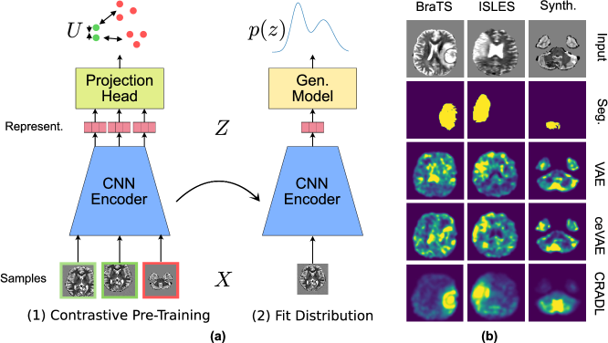
Figure 1: (a) Visualization of the fitting pipeline, from contrastive pretext (SimCLR) (1) to fitting of the generative model (2). (b) Pixel-wise scores - clamped and normalized for visual inspection.

3.1 Contrastive Training

During the first stage of training CRADL, a contrastive pretext-task is used to train the encoder. The contrastive task we use is conceptually identical to SimCLR [14] but uses different data augmentations changed for the medical domain as transformations. When using SimCLR, positive pairs are obtained using data augmentations $t$ drawn randomly from a set of augmentations $\mathcal{T}$ and all other pairs of the samples are used as negatives. To this end, each sample $x_{i}$ in a minibatch of $N$ examples is transformed twice, yielding two different views that make up the positive pair. The representations produced by feeding the views through the encoder $f$ and projection head $g$, $\tilde{u}_{i}=g(f(\tilde{t}(x_{i})))$ and $\hat{u}_{i}=g(f(\hat{t}(x_{i})))$, are encouraged to be similar by optimizing the NT-Xent contrastive loss:

$$L(x_{i})=-\log\dfrac{\exp(\text{sim}(\tilde{u}_{i},\hat{u}_{i})/\tau)}{\sum_{\bar{u}\in\Lambda^{-}}\exp(\text{sim}(\tilde{u}_{i},\bar{u}))/\tau)}$$ (4)

Here the set $\Lambda^{-}$ are the negative pairs for a sample $x_{i}$ consisting of all examples except $\tilde{u}_{i}$, which are all other $2N-1$ examples in the minibatch. The similarity measure $\text{sim}(x,y)$ is cosine similarity. The loss over the whole minibatch is then obtained by summing over all positive pairs.

3.2 Generative Model

The generative model operating on the representation space to detect and localize anomalies, which is trained in the second stage, can be essentially any generative model. In practice, there just needs to be a selection or aggregation criterion. However, due to the encoder’s clustered representations, a ‘simple’ generative model can be used. Concretely we decide to use two families being:

Gaussian Mixture Model A Gaussian Mixture Model (GMM) is used since it is one of the simplest generative models. The probability distribution of a GMM with $K$ components is noted in equation 5. We fit the GMM with the Expectation-Maximization (EM) Algorithm [28] with $K$ being the number of components (specified before the fit).

$$p(z;\Theta)=\sum_{k=1}^{K}\mathcal{N}(z;\mu_{k},\Sigma_{k})\cdot\pi_{k}$$ (5)

Here $\mu_{k}$ is the mean, $\Sigma_{k}$ is the covariance matrix and $\pi_{k}$ is the bias of mode $k$.

Normalizing Flow A simple Normalizing Flow (Flow) based on the invertible and volume-preserving RealNVP architecture [29] is used since it allows to model complex probability distributions. This is achieved through the use of the change of variable formula in combination with a standard normal (Gaussian) $\mathcal{N}(0,\text{I})$ with the same dimensionality as $Z$ as a prior in its latent space

$$p(z;\Theta)=\mathcal{N}(\text{Flow}(z);0,\text{I})\cdot\left|\det\left(\text{Jacobian}_{\text{Flow}}(z)\right)\right|.$$ (6)

The Normalizing Flow should be able to give an upper limit to the performance achievable with GMMs with more components.

4 Experimental Setup

All experiments were performed three times with different seeds to obtain a mean and standard deviation explicitly stated for all experimental results.

4.1 Datasets

All our experiments are conducted on T2-weighted MRI brain datasets consisting of 3D medical images. All datasets are pre-processed similarly, with the final step being image-wise z-score normalization of each image and clipping the intensity from -1.5 to 1.5 following [13]. For use with our models, the 3D images are sliced along the z-axis and are used as 2D inputs, which are then resized to a resolution of 128x128. This approach to reducing the complexity of the volumetric data and pre-processing is standard procedure [6, 13]

Training Dataset

For training all of our models, we use a subset of the HCP dataset [30], which purely consists of ‘normal’ MRI Scans, using 894 scans split into training and validation sets. The HCP dataset consists of young and healthy adults taken in a scientific study.

Anomalous Datasets

We use three anomalous datasets with test and validation sets for score selection to evaluate the anomaly detection and localization performance, all showcasing a 100% anomaly prevalence per image based on the presence of a tumor or diseased area in the segmentation mask. These three datasets are:

HCP Synth. An artificially created anomalous dataset we created based on the leftover 98 images from the HCP dataset (not used for training) by rendering real-world objects into brain regions as anomalies following the approach by [31]. This allows the test set to have the same original distribution (i.e., population, same scanner, site, registration…) as the training set, with only the anomalies differing.

ISLES The ischemic stroke lesion segmentation challenge 2015 (ISLES) dataset [32] with anomalous regions being the stroke lesions consisting of 28 scans taken from 2 institutions during clinical routine. This dataset is explicitly stated to contain different pathologies which are not annotated.

BraTS The Brain Tumor Segmentation Challenge 2017 (BraTS) dataset [33] with anomalous regions being glioblastoma and lower grade glioma consisting of 286 scans taken from multiple institutions during clinical routine.

To allow better interpretation of our results, we give a short dataset description with values for interpreting the results for anomaly detection based on slices and anomaly localization based on voxels can be seen in Tab. 1.

Level	Scans		Slices				Voxels
Value	# in Dataset		# in Dataset		Anomaly Prevalence		Anomaly Prevalence
Dataset	Test	Val.	Test	Val	Test	Val	Test	Val
HCP Synth.	49	49	7105	7105	20.5%	19.8%	0.649%	0.770%
ISLES	20	8	2671	1069	36.6%	34.1%	1.140%	1.099%
BraTS	266	20	35910	2700	49.0%	46.0%	2.427%	1.923%

Table 1: Statistically relevant characteristics of the anomalous datasets used in our evaluation. The baseline AUPRC of a random score is equal to the prevalence.

Distribution Shifts

Several distribution shifts from the HCP dataset created for scientific purposes to clinical datasets ISLES and BraTS lead to different intensity histograms and prevalences on slice and voxel levels. Firstly, a population shift is present due to the high prevalence of disease in both clinical datasets which is much higher than that of the whole human population and also often correlated with the age of the population. Therefore are not only unannotated anomalies present in images from BraTS and ISLES but also structural changes due to the different ages of the underlying populations of the datasets. Secondly, a shift in the images is present due to different scanners used to take the images. Generally, the scans for the scientific HCP dataset are taken with an MRI-Scanner with a higher magnetic field strength than used in clinical practice for both BraTS and ISLES.

4.2 Model

We use a unified model architecture for our experiments which is based on the deep convolutional architecture from [34], so our encoder solely consists of 2D-Conv-Layers and our decoder (for the VAE models) of 2D-Transposed-Conv-Layers (for more details, please refer to the Appendix). We chose an initial feature map size of 64 and a latent dimension of 512. For the projection head of CRADL, we use a simple 2-layer MLP with ReLU non-linearities, a 512 dim. hidden layer, and 256 dim. output. We performed for both our baselines and our proposed method experiments with different bottleneck sizes and feature map counts.

4.3 Training CRADL

Contrastive Pretext-Task

The contrastive pretext training of the encoder is performed for 100 epochs on the HCP training set using the Adam Optimizer, a learning rate of 1e-4, Cosine Annealing [35], 10 Warm-up Epochs and a weight decay of 1e-6, the temperature of the contrastive loss is 0.5 [14]. The encoder for later evaluation is selected based on the smallest loss on the HCP validation set. As transformations for generating different views for the contrastive task, we use a combination of random cropping, random scaling, random mirroring, rotations, and multiplicative brightness, and Gaussian noise.

Generative Model

We fit a batch of GMMs with $K\in\{1,2,4,8\}$ on representations of the encoder from all samples in the HCP training set without any augmentation. The means of the components are randomly initialized, and the convergence limit for the EM algorithm is set to $0.1$. In the Appendix, we present the performance of CRADL in relation to $K$.

The Normalizing Flow is also trained on the representation space in the same manner as the GMM to maximize the likelihood of the samples [29]. All further information regarding the exact training process and model architecture are shown in the Appendix.

4.4 Baselines

We train both the VAE and ceVAE for 100 epochs using the Adam Optimizer, a learning rate of 1e-4, and the unified architecture for both the encoder and decoder on the HCP training dataset. The final models for evaluation are chosen based on the lowest loss on the HCP validation set. The transformations we use during training of the VAE consist of random scaling, random mirroring, rotations, multiplicative brightness, and Gaussian noise, which have shown clear performance improvements in our early experiments. For the ceVAE, we add random cutout transformations [13].

4.5 Inference

We select the best scoring function for CRADL and all baselines concerning each anomalous evaluation dataset based on the best validation set AUPRC metric (see Appendix). For CRADL, the scoring functions are the different generative models on its representations. For the VAE and ceVAE, these are the different terms of the loss (Reconstruction difference (Rec.)[16], KL-Divergence [13], ELBO/combi[13, 16]). We deem this approach of scoring function selection reasonable and motivate the choice of generative model selection for CRADL by the fact that the fit of all GMMs and the Normalizing Flow on representations take only 50 minutes on one GPU together compared to more than 8 hours for the fit of one VAE or ceVAE.

Post-processing of Anomaly Heatmaps

The post-processing pipeline for the pixel-level scores is identical for all methods evaluated and, based on the approach from [6], restricted to only use one sample (2D): We zero out all pixel scores outside the brain region. In the next step, 2D median pooling (kernel size=5) is applied to filter out edges and single outliers. As the last step, Gaussian smoothing is applied, inspired by the finding of sparse gradients and convolutional artifacts by [13]. Empirically, the reconstruction-based scores of the VAE and ceVAE benefited from this step.

4.6 Evaluation Metrics

For the two different tasks of anomaly detection and localization, the discriminative power of the scoring function is measured using the Area Under the Receiver Operator Curve (AUROC) and the Area Under the Precision-Recall Curve (AUPRC) due to their independence of a threshold with anomalies being defined as positives. In our setting, it is more critical to detect outliers than inliers in combination with a larger number of normal slices/voxels than anomalous slices/voxels. Hence, we emphasize the importance of the AUPRC score because it better captures the detection of anomalies.

For anomaly detection, we aggregate all slices of a dataset, and each slice is seen as anomalous if more than five voxels contain an anomaly.

For anomaly localization, we aggregate the anomaly heatmaps of all slices and the corresponding ground-truth segmentations.

5 Results & Discussion

First, we analyze the performance of CRADL for anomaly detection and localization with our re-implementations of the state-of-the-art methods VAE and ceVAE [6, 13] in sections 5.1 and 5.2. Then, we analyze the discriminative power of the representations obtained with contrastive learning to that of the aforementioned generative models in the context of anomaly detection and localization in 5.3.

The results of every scoring method of each anomaly detection and localization approach are shown in the Appendix, whereas in the following subsections, only relevant results are portrayed.

5.1 Comparison to State-of-the-Art for Anomaly Detection

Method	HCP Synth.		ISLES		BraTS
	AUPRC	AUROC	AUPRC	AUROC	AUPRC	AUROC
CRADL	77.8(0.7)	89.8(0.3)	54.9(0.5)	69.3(0.0)	81.9(0.2)	82.6(0.3)
ceVAE	43.2(0.2)	76.9(0.1)	54.1(0.8)	72.7(0.1)	85.6(0.2)	86.5(0.1)
VAE	48.5(0.9)	79.4(0.1)	51.9(0.6)	71.7(0.2)	80.7(0.7)	83.3(0.6)

Table 2: Slice-wise anomaly detection performance. AUROC and AUPRC are given in: mean(standard deviation)%

By comparing CRADL with our re-implementations of the VAE and ceVAE for slice-wise anomaly detection, we want to assess the general performance of our approach to that of state-of-the-art baselines. The results are shown in Tab. 2. For the HCP Synth. dataset CRADL substantially outperforms both the VAE and ceVAE. On both ISLES and BRATS, the ceVAE is the best-performing approach showcasing the advantage of the additional self-supervised task on ISLES, whereas it is tied with the VAE on BraTS.

Due to the aforementioned distribution shifts from the normal (healthy) population on HCP to ISLES and BraTS and the more diverse and subtle set of anomalies on HCP Synth. we conclude, therefore, that CRADL can capture fine deviations from normality better than a VAE and ceVAE. And it can be hypothesized that this exact property of CRADL being able to capture delicate deviations from normality better than a VAE and ceVAE might be the reason for it performing worst on ISLES and BraTS since, based on a distribution perspective, essentially all slices from ISLES and BraTs could be considered anomalous.

This hypothesis could also be backed up since on HCP Synth. the best performing scoring methods are based on the GMM with 8 components and the Normalizing Flow, which both should be able to capture even relatively complex distributions well, while for ISLES and BraTS the GMM with 1 component leads to the best anomaly detection performance where the latter is not as well suited to capture the fine difference in the representation space than the former.

5.2 Comparison to State-of-the-Art Anomaly Localization

Method	HCP Synth.		ISLES		BraTS
	AUPRC	AUROC	AUPRC	AUROC	AUPRC	AUROC
CRADL	32.5(0.8)	97.8(0.0)	18.6 (3.9)	89.8(0.3)	38.0(1.6)	94.2(0.1)
ceVAE	17.2(1.5)	92.1(0.4)	14.5(1.3)	87.9 (0.2)	48.3(3.0)	94.8(0.3)
VAE	24.9(0.6)	95.5(0.1)	7.7(1.2)	87.5 (0.6)	29.8(0.4)	92.5(0.1)

Table 3: Voxel-wise anomaly localization performance. AUROC and AUPRC are given in: mean(standard deviation)%

The goal of this experiment is to verify the effectiveness of our approach for anomaly localization by backpropagating gradients of the NLL of generative models operating on a representation space to the image space through an encoder. To this end, we compare our results again with our state-of-the-art implementations of a VAE and ceVAE each with three different scores, which are reconstruction differences, backpropagated gradients of the KL-Divergence [13] and the combi-scoring based on a multiplication of KL-Divergence gradients and reconstruction differences [13]. The results of the best-performing anomaly localization scoring methods for CRADl, VAE and ceVAE are shown in Tab. 3. On HCP Synth. and ISLES CRADL outperforms both VAE and ceVAE. On the BraTS dataset, the ceVAE is the best-performing method followed by the VAE. The trend already discussed in Sec. 5.1 continues where HCP Synth. favors for CRADL more complex generative models with the performance increasing, for higher values of K. Interestingly the Normalizing Flow does not perform well, but this might be due to convoluted gradients in the representation space, which do not behave as ‘nice’ as the one of a GMM approximately scaling quadratically with regard to Mahalanobis distance from a center. The trend that using representations for anomaly localization is advantageous can be observed for the VAE and ceVAE where the combi-score performs best by combining both information from the representation and the prior distribution with the reconstruction error by defining a distribution in image space [13]. Further, the fact that CRADL performs not as much better on ISLES and worse on BraTS than the ceVAE might be due to the context-encoding task better suited to these datasets where anomalies regions are lesions that often glow brightly in T2-weighted MRI scans.

We interpret the strong results on HCP Synth for anomaly localization to showcase that CRADL can localize anomalies that are close to the normal distribution and diverse in appearance (not only bright glowing) better than both ceVAE and VAE.

5.3 Anomaly Detection & Localization with Generative Models on Representation

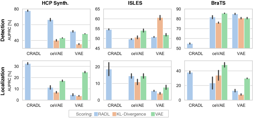
Figure 2: Performance comparison of CRADL with representation-based anomaly detection and localization (RADL) on the ceVAE and VAE alongside the KL-Divergence and the best VAE scoring method to assess the performance of purely representation-based approaches in general and the advantage of contrastive representations.

This experiment was performed to assess two things with regard to the down-stream tasks of anomaly detection and localization. Firstly, whether purely representation-based anomaly scoring for the generative methods VAE and ceVAE offers advantages over standard anomaly scoring. To this end, we define the representation-based anomaly detection and localization approach (RADL) where the use of a generative model on the representations of CRADL (see Sec. 3.2) is emulated on the representations of a VAE and ceVAE. Secondly, we want to assess whether the contrastive representations of CRADL are better suited for the two aforementioned down-stream tasks than the representations of generative models (generative pretext-task).

Tackling both questions, we depict both anomaly detection and localization performance in Fig. 2, where we followed the score selection criterion detailed in Sec. 4. Regarding the effectiveness of the purely representation-based RADL on the VAE and ceVAE, we compare it with the KL-Divergence and the best VAE scoring method selected in sections 5.1 & 5.2. For Anomaly Localization it improves the performance over the KL-Divergence on BraTS and on HCP Synth it improves upon the best-performing VAE scoring method while underperforming on ISLES. For Anomaly Detection the RADL approach leads to substantial performance improvements over the KL-Divergence in all cases except for the ceVAE on BraTS, but it never outperforms the VAE scoring methods also using reconstruction.

Based on these results we conclude that the RADL approach for generative methods using the representations yields performance benefits over the KL-Divergence and allows to detection of fine differences in the distribution as showcased by the results on HCP Synth..

Regarding the second point, assessing our hypothesis regarding performance benefits of the contrastive representations of CRADL, due to carrying more semantic information, compared with generative representations. We see our results as strengthening our hypothesis due to the clear performance improvements of CRADL for anomaly localization over the KL-Divergence and RADL approaches for anomaly localization and the performance improvement on HCP Synth. over the ceVAE and VAE performance as well as on ISLES with the exception of the KL-Divergence of the VAE. Even though, CRADL has the worst performance on BraTS for anomaly detection is directly counteracting our hypothesis. We argue again that this behavior might stem from the distribution shift already mentioned and that the contrastive representations allow for better detection and localization of fine semantic differences between anomalous and normal brain volumes as the HCP Synth. dataset provides A further supporting fact of the advantage of a self-supervised pretext task is that the ceVAE, which also employs a self-supervised task, outperforms the VAE.

5.4 Caveat of Experimental Setup

Our experimental evaluations suffer from either being a synthetic problem for HCP synth. or the distribution shifts of BraTS and ISLES discussed in section 4.1. We believe that the experimental evidence on HCP synth. is the most trustworthy with regard to the specific task since structural changes due to age and unannotated anomalies in BraTS and ISLES do not allow showcasing the performance benefits of certain methods over others.

Another critical aspect of the whole field, in general, is the high prevalence of anomalous cases during evaluation since this might lead to the possibility of methods being favored in evaluation metrics if giving per se high scores to certain regions of the brain prone to anomalies (here lesions). This aspect would need to be assessed either directly or evaluated by also having many normal images in the test datasets.

6 Conclusion

In this work, we propose to purely use representations for unsupervised anomaly detection and localization and investigate to this end contrastive representations of a SimCLR-like pretext task. CRADL a simple framework for unsupervised anomaly detection and localization is the result of this investigation.

Concretely, we have shown that purely representation-based anomaly detection has benefits over generative models operating on image space and that representations of an encoder, trained with a contrastive pretext-task, in combination with a simple generative model, show advantageous properties over generative models on image space leading to better performance in the context anomaly detection and localization. This could clearly be observed for fine and diverse deviations from the distribution of normal samples. For anomaly detection, slightly more powerful generative models like the normalizing flow operating on the representation space seem to perform best. Whereas for anomaly localization, simpler generative models like a GMM perform better.

We believe the following two use cases make good use CRADL’s properties for anomaly detection and localization:

- Cases with an Abundance of unannotated healthy and diseased images since the representation learning approach is decoupled from distribution learning. Further, it has been shown that using anomalous data for the pretext-task can even be helpful [17] for a VQ-VAE.

- Cases with a small healthy/normal dataset due to the low-dimensionality reducing the number of samples needed for the fit of the distribution with simpler generative models compared to generative modeling on image space.

To increase the potential use case for the medical domain a generalization to 3D inputs would be necessary and aggregation schemes for cases where a whole needs to be processed in smaller pieces s.a. the slice-wise approach here. Further, since the approach of representation-based anomaly detection itself is very general as showcased by the experiments in Sec. 5.3, we believe that other self-supervised tasks [36, 37] might further increase the performance of CRADL. Also, restorative techniques s.a. image restoration [7] and representation resampling [17, 18] might also be incorporated into the CRADL approach.

Anomaly detection and localization is a promising research field for the medical imaging domain, due to its potential to alleviate the annotation burden for medical screenings using deep learning to take place while having similar and understood properties to standard medical tests s.a. the blood count. We hope that our proposed method and insights help push anomaly detection and localization into clinical practice.

Appendix A Results

All results using all scoring methods for all anomaly detection and localization approaches are shown here. In Tab. 4 the selected scoring methods shown in Sec. 5 are displayed. For slice-wise anomaly detection the validation and test set performance is shown in Tab. 8 and Tab. 7. For voxel-wise anomaly localization the validation and test set performance is shown in Tab. 6 and Tab. 5.

Dataset	Method	Anomaly Detection		Anomaly Localization
		Section 5.1	Section 5.3	Section 5.2	Section 5.3
HCP Synth.	CRADL	Norm. Flow	Norm. Flow	GMM 8	GMM 8
	VAE	ELBO	GMM 8	combi	GMM 8
	ceVAE	ELBO	Norm. Flow	combi	GMM 8
BraTS	CRADL	GMM 1	GMM 1	GMM 2	GMM 2
	VAE	KL-Div	GMM 8	rec	GMM 4
	ceVAE	ELBO	GMM 1	combi	GMM 1
ISLES	CRADL	GMM 1	GMM 1	GMM 1	GMM 1
	VAE	ELBO	GMM 8	combi	GMM 1
	ceVAE	ELBO	GMM 1	combi	GMM 1

Table 4: Model Selection for all results shown in Sec. 5 based on validation set performance shown in Tabs. 8 and 6

			HCP Synth.		BraTS		ISLES
Pre-Text	Gen. Model	Score	AUPRC	AUROC	AUPRC	AUROC	AUPRC	AUROC
VAE	GMM 1 Comp	NLL-grad	0.0236$\pm$0.0011	0.8501$\pm$0.0035	0.1282$\pm$0.0123	0.8889$\pm$0.0023	0.0563$\pm$0.0033	0.86$\pm$0.0016
	GMM 2 Comp	NLL-grad	0.0206$\pm$0.0006	0.8436$\pm$0.0022	0.1095$\pm$0.0096	0.8808$\pm$0.0021	0.0471$\pm$0.0024	0.8523$\pm$0.0036
	GMM 4 Comp	NLL-grad	0.0348$\pm$0.004	0.8851$\pm$0.0054	0.1295$\pm$0.0173	0.8918$\pm$0.0038	0.0562$\pm$0.0057	0.8578$\pm$0.0035
	GMM 8 Comp	NLL-grad	0.048$\pm$0.0086	0.9019$\pm$0.007	0.1345$\pm$0.013	0.8949$\pm$0.0026	0.0584$\pm$0.0058	0.8605$\pm$0.0028
	Norm. Flow	NLL-grad	0.04$\pm$0.0066	0.8885$\pm$0.0077	0.0978$\pm$0.012	0.8666$\pm$0.009	0.0498$\pm$0.0098	0.8516$\pm$0.0048
	VAE	combi	0.2491$\pm$0.0063	0.9546$\pm$0.0005	0.2269$\pm$0.0328	0.9198$\pm$0.0038	0.077$\pm$0.0122	0.8745$\pm$0.0059
		KL-Div.-grad	0.0373$\pm$0.0032	0.8657$\pm$0.0014	0.0772$\pm$0.0091	0.8446$\pm$0.011	0.0409$\pm$0.0047	0.8466$\pm$0.0081
		Rec.	0.2101$\pm$0.003	0.9511$\pm$0.0003	0.2976$\pm$0.0035	0.9248 $\pm$0.0006	0.0513$\pm$0.0001	0.8532$\pm$0.0023
ceVAE	GMM 1 Comp	NLL-grad	0.1072$\pm$0.0109	0.901$\pm$0.01	0.2343$\pm$0.0816	0.9129$\pm$0.0159	0.0618 $\pm$0.0176	0.86$\pm$0.0089
	GMM 2 Comp	NLL-grad	0.0757$\pm$0.0057	0.8952$\pm$0.0041	0.177$\pm$0.0426	0.9062$\pm$0.0097	0.0449$\pm$0.0093	0.8445$\pm$0.0068
	GMM 4 Comp	NLL-grad	0.0967$\pm$0.0156	0.9116$\pm$0.0085	0.1906$\pm$0.0184	0.9105$\pm$0.004	0.0511$\pm$0.0123	0.8456$\pm$0.006
	GMM 8 Comp	NLL-grad	0.1122$\pm$0.016	0.9223$\pm$0.0058	0.2068$\pm$0.033	0.9119$\pm$0.006	0.0612$\pm$0.0084	0.8488$\pm$0.0055
	Norm. Flow	NLL-grad	0.0606$\pm$0.0148	0.9008$\pm$0.0101	0.1072$\pm$0.0159	0.8756$\pm$0.0079	0.0304$\pm$0.0007	0.8157$\pm$0.0013
	VAE	combi	0.1716$\pm$0.0146	0.9212$\pm$0.004	0.483$\pm$0.0299	0.9482$\pm$0.0032	0.1451$\pm$0.0125	0.8794$\pm$0.0022
		KL-Div.-grad	0.0702$\pm$0.0069	0.8586$\pm$0.0047	0.3394$\pm$0.067	0.9252$\pm$0.0163	0.1085$\pm$0.0163	0.8785$\pm$0.0059
		Rec.	0.0913$\pm$0.0023	0.9266$\pm$0.0017	0.4073$\pm$0.0389	0.9269$\pm$0.0074	0.0653$\pm$0.0044	0.8544$\pm$0.005
CRADL	GMM 1 Comp	NLL-grad	0.2263$\pm$0.0112	0.9664$\pm$0.0017	0.3341$\pm$0.0402	0.9357$\pm$0.0035	0.1859$\pm$0.0385	0.8977$\pm$0.0033
	GMM 2 Comp	NLL-grad	0.2243$\pm$0.0125	0.9685$\pm$0.0017	0.3802$\pm$0.0163	0.9418$\pm$0.0009	0.1653$\pm$0.02	0.8955$\pm$0.0029
	GMM 4 Comp	NLL-grad	0.2875$\pm$0.0101	0.9741$\pm$0.0006	0.3383$\pm$0.0161	0.9384$\pm$0.0012	0.1441$\pm$0.0024	0.8935$\pm$0.003
	GMM 8 Comp	NLL-grad	0.3246$\pm$0.0076	0.9779$\pm$0.0003	0.2908$\pm$0.0199	0.9309$\pm$0.0022	0.1257$\pm$0.0151	0.8906$\pm$0.0019
	Norm. Flow	NLL-grad	0.0924$\pm$0.0097	0.9397$\pm$0.0031	0.1362$\pm$0.0102	0.8736$\pm$0.0068	0.0393$\pm$0.0044	0.8213$\pm$0.0153

Table 5: Voxel-Wise anomaly localization metrics on test datasets. Values are shown in the Results & Discussion section and selected based on the results of the best AUPRC scores on the validation set (Tab. 6)

			HCP Synth.		BraTS		ISLES
Pre-Text	Gen. Model	Score	AUPRC	AUROC	AUPRC	AUROC	AUPRC	AUROC
VAE	GMM 1	NLL-grad	0.0353$\pm$0.0056	0.8547$\pm$0.0025	0.0935$\pm$0.0047	0.8841$\pm$0.0022	0.0676$\pm$0.0149	0.8745$\pm$0.0095
	GMM 2	NLL-grad	0.0276$\pm$0.0018	0.8487$\pm$0.0031	0.0799$\pm$0.0046	0.8751$\pm$0.0038	0.0548$\pm$0.0102	0.8632$\pm$0.0067
	GMM 4	NLL-grad	0.0503$\pm$0.0071	0.8859$\pm$0.0043	0.1009$\pm$0.0131	0.8897$\pm$0.0058	0.0627$\pm$0.0064	0.8701$\pm$0.0032
	GMM 8	NLL-grad	0.0774$\pm$0.0035	0.9088$\pm$0.0023	0.0925$\pm$0.0073	0.8875$\pm$0.0041	0.0624$\pm$0.0029	0.8805$\pm$0.0006
	Norm. Flow	NLL-grad	0.0395$\pm$0.0008	0.8665$\pm$0.0021	0.0691$\pm$0.0036	0.8584$\pm$0.0052	0.0509$\pm$0.0091	0.863$\pm$0.0091
	VAE	combi	0.2945$\pm$0.0059	0.9527$\pm$0.0005	0.1842$\pm$0.0403	0.9171$\pm$0.0061	0.0894$\pm$0.012	0.8812$\pm$0.0051
		KL-Div.-grad	0.0735$\pm$0.0012	0.8771$\pm$0.0007	0.0677$\pm$0.0096	0.8553$\pm$0.0131	0.041$\pm$0.0009	0.8456$\pm$0.0044
		Rec.	0.2081$\pm$0.0042	0.9426$\pm$0.0004	0.2248$\pm$0.0077	0.9119$\pm$0.0015	0.0543$\pm$0.0082	0.8618$\pm$0.0056
ceVAE	GMM 1	NLL-grad	0.1212$\pm$0.024	0.9057$\pm$0.0111	0.2313$\pm$0.0829	0.9181$\pm$0.0138	0.0609$\pm$0.0166	0.8633$\pm$0.0059
	GMM 2	NLL-grad	0.0741$\pm$0.0142	0.8989$\pm$0.0065	0.1611$\pm$0.0291	0.9126$\pm$0.0051	0.0385$\pm$0.0056	0.8436$\pm$0.005
	GMM 4	NLL-grad	0.1067$\pm$0.0132	0.9167$\pm$0.0039	0.1955$\pm$0.0214	0.9163$\pm$0.0024	0.0423$\pm$0.0058	0.8513$\pm$0.0033
	GMM 8	NLL-grad	0.1464$\pm$0.0285	0.9286$\pm$0.007	0.1841$\pm$0.0162	0.911$\pm$0.0002	0.0404$\pm$0.0054	0.8471$\pm$0.0044
	Norm. Flow	NLL-grad	0.0907$\pm$0.0144	0.9002$\pm$0.0081	0.0784$\pm$0.0144	0.8681$\pm$0.0088	0.0311$\pm$0.0017	0.8223$\pm$0.0094
	VAE	combi	0.2183$\pm$0.0206	0.9148$\pm$0.0057	0.4321$\pm$0.005	0.9393$\pm$0.0038	0.1628$\pm$0.0242	0.8847$\pm$0.0042
		KL-Div.-grad	0.096$\pm$0.0096	0.8655$\pm$0.0037	0.3337$\pm$0.04	0.9317$\pm$0.0078	0.0956$\pm$0.0278	0.8751$\pm$0.0092
		Rec.	0.1163$\pm$0.0019	0.9117$\pm$0.0021	0.2884$\pm$0.0403	0.9068$\pm$0.0088	0.1321$\pm$0.029	0.8649$\pm$0.0041
VAE	GMM 1	NLL-grad	0.3309$\pm$0.0064	0.969$\pm$0.0013	0.3102$\pm$0.0129	0.9364$\pm$0.0007	0.3279$\pm$0.0096	0.9342$\pm$0.0027
	GMM 2	NLL-grad	0.3184$\pm$0.0063	0.9688$\pm$0.0012	0.3748$\pm$0.0129	0.942$\pm$0.0016	0.3523$\pm$0.0034	0.9259$\pm$0.0034
	GMM 4	NLL-grad	0.3269$\pm$0.0058	0.9698$\pm$0.0012	0.3284$\pm$0.0095	0.9369$\pm$0.0014	0.3173$\pm$0.0246	0.9175$\pm$0.0032
	GMM 8	NLL-grad	0.3354$\pm$0.0085	0.9725$\pm$0.001	0.3179$\pm$0.0091	0.9376$\pm$0.0025	0.2908$\pm$0.0242	0.9187$\pm$0.0017
	Norm. Flow	NLL-grad	0.1176$\pm$0.004	0.9297$\pm$0.0043	0.1474$\pm$0.0152	0.8943$\pm$0.0052	0.1159$\pm$0.0235	0.8781$\pm$0.0123

Table 6: Pixel-Wise anomaly localization metrics on validation datasets. Values show the scoring methods with the highest AUPRC scores.

			HCP Synth.		BraTS		ISLES
Pre-Text	Gen. Model	Score	AUPRC	AUROC	AUPRC	AUROC	AUPRC	AUROC
VAE	GMM 1	NLL	0.3710 $\pm$ 0.0083	0.7238 $\pm$ 0.0072	0.8254 $\pm$ 0.0079	0.8481 $\pm$ 0.0034	0.5121 $\pm$ 0.0050	0.7093 $\pm$ 0.0007
	GMM 2	NLL	0.3516 $\pm$ 0.0056	0.7229 $\pm$ 0.0060	0.8054 $\pm$ 0.0076	0.8351 $\pm$ 0.0041	0.4812 $\pm$ 0.0066	0.6783 $\pm$ 0.004
	GMM 4	NLL	0.4383 $\pm$ 0.0104	0.7748 $\pm$ 0.0054	0.8271 $\pm$ 0.0051	0.8467 $\pm$ 0.0029	0.4766 $\pm$ 0.0076	0.6824 $\pm$ 0.0081
	GMM 8	NLL	0.5164 $\pm$ 0.0087	0.7961 $\pm$ 0.0044	0.8495 $\pm$ 0.0062	0.8574 $\pm$ 0.0030	0.5077 $\pm$ 0.0024	0.7059 $\pm$ 0.0033
	Norm. Flow	NLL	0.5422 $\pm$ 0.0129	0.8010 $\pm$ 0.0050	0.8293 $\pm$ 0.0089	0.8462 $\pm$ 0.0051	0.4882 $\pm$ 0.0024	0.6838 $\pm$ 0.0075
	VAE	ELBO	0.4853 $\pm$ 0.0041	0.7941 $\pm$ 0.0010	0.8546 $\pm$ 0.0010	0.8647 $\pm$ 0.0007	0.5188 $\pm$ 0.0055	0.7174 $\pm$ 0.0022
		KL-Div.	0.3536 $\pm$ 0.0059	0.7294 $\pm$ 0.0020	0.8073 $\pm$ 0.0069	0.8329 $\pm$ 0.0050	0.6068 $\pm$ 0.0124	0.7612 $\pm$ 0.0030
		Rec.	0.4889 $\pm$ 0.004	0.7983 $\pm$ 0.0009	0.8521 $\pm$ 0.0008	0.8640 $\pm$ 0.0008	0.5126 $\pm$ 0.0065	0.7108 $\pm$ 0.0026
ceVAE	GMM 1	NLL	0.4758 $\pm$ 0.0271	0.7893 $\pm$ 0.0113	0.8173 $\pm$ 0.0147	0.8456 $\pm$ 0.0079	0.4967 $\pm$ 0.0191	0.6857 $\pm$ 0.0083
	GMM 2	NLL	0.4892 $\pm$ 0.0371	0.7958 $\pm$ 0.0133	0.7518 $\pm$ 0.0286	0.8063 $\pm$ 0.0094	0.3924 $\pm$ 0.022	0.5836 $\pm$ 0.0176
	GMM 4	NLL	0.5287 $\pm$ 0.0371	0.8076 $\pm$ 0.0123	0.8013 $\pm$ 0.0268	0.8308 $\pm$ 0.0147	0.4098 $\pm$ 0.0186	0.5981 $\pm$ 0.0246
	GMM 8	NLL	0.5900 $\pm$ 0.0328	0.8233 $\pm$ 0.0101	0.7824 $\pm$ 0.0395	0.8211 $\pm$ 0.0175	0.3824 $\pm$ 0.0415	0.5696 $\pm$ 0.0463
	Norm. Flow	NLL	0.6642 $\pm$ 0.0162	0.8452 $\pm$ 0.0091	0.7296 $\pm$ 0.043	0.7700 $\pm$ 0.0285	0.4005 $\pm$ 0.0185	0.5976 $\pm$ 0.0277
	VAE	ELBO	0.4321 $\pm$ 0.0021	0.7691 $\pm$ 0.0010	0.8556 $\pm$ 0.0019	0.8653 $\pm$ 0.0009	0.5412 $\pm$ 0.0082	0.7266 $\pm$ 0.0008
		KL-Div.	0.4022 $\pm$ 0.0100	0.7547 $\pm$ 0.0046	0.7612 $\pm$ 0.0063	0.8024 $\pm$ 0.0033	0.5064 $\pm$ 0.0071	0.6967 $\pm$ 0.0088
		Rec.	0.4294 $\pm$ 0.0036	0.7683 $\pm$ 0.0007	0.8563 $\pm$ 0.0023	0.8660 $\pm$ 0.0012	0.5467 $\pm$ 0.009	0.7279 $\pm$ 0.0003
CRADL	GMM 1	NLL	0.6988 $\pm$ 0.0032	0.8679 $\pm$ 0.0024	0.8187 $\pm$ 0.0024	0.8264 $\pm$ 0.0010	0.5488 $\pm$ 0.0049	0.6927 $\pm$ 0.0003
	GMM 2	NLL	0.7043 $\pm$ 0.0044	0.8733 $\pm$ 0.0023	0.7913 $\pm$ 0.0026	0.7967 $\pm$ 0.0011	0.4891 $\pm$ 0.0048	0.6367 $\pm$ 0.0020
	GMM 4	NLL	0.7538 $\pm$ 0.0027	0.8856 $\pm$ 0.0019	0.7787 $\pm$ 0.0030	0.7867 $\pm$ 0.0012	0.4831 $\pm$ 0.0001	0.6369 $\pm$ 0.0030
	GMM 8	NLL	0.7598 $\pm$ 0.0034	0.8871 $\pm$ 0.0021	0.7949 $\pm$ 0.0034	0.8010 $\pm$ 0.0017	0.5028 $\pm$ 0.0038	0.6441 $\pm$ 0.0011
	Norm. Flow	NLL	0.7777 $\pm$ 0.0069	0.8979 $\pm$ 0.0027	0.6883 $\pm$ 0.0145	0.7163 $\pm$ 0.0139	0.4427 $\pm$ 0.0185	0.6289 $\pm$ 0.0212

Table 7: Slice-Wise anomaly detection metrics on test datasets. Values are shown in the Results & Discussion section and selected based on the results of the best AUPRC scores on the validation set (Tab. 8)

			HCP Synth.		BraTS		ISLES
Pre-Text	Gen. Model	Score	AUPRC	AUROC	AUPRC	AUROC	AUPRC	AUROC
VAE	GMM 1	NLL	0.4214 $\pm$ 0.0057	0.7269 $\pm$ 0.0054	0.8068 $\pm$ 0.0162	0.8463 $\pm$ 0.0032	0.7408 $\pm$ 0.0065	0.8450 $\pm$ 0.0036
	GMM 2	NLL	0.4120 $\pm$ 0.0052	0.7269 $\pm$ 0.0053	0.7899 $\pm$ 0.0128	0.8273 $\pm$ 0.0019	0.7149 $\pm$ 0.0022	0.8130 $\pm$ 0.0015
	GMM 4	NLL	0.4479 $\pm$ 0.0065	0.7613 $\pm$ 0.0035	0.8117 $\pm$ 0.0147	0.8342 $\pm$ 0.0086	0.6913 $\pm$ 0.0167	0.8042 $\pm$ 0.0105
	GMM 8	NLL	0.5236 $\pm$ 0.0105	0.7890 $\pm$ 0.0046	0.8304 $\pm$ 0.0156	0.8506 $\pm$ 0.0064	0.7487 $\pm$ 0.0072	0.8353 $\pm$ 0.0041
	Norm. Flow	NLL	0.5126 $\pm$ 0.0074	0.7800 $\pm$ 0.0091	0.8024 $\pm$ 0.0050	0.8321 $\pm$ 0.0031	0.7184 $\pm$ 0.0165	0.8149 $\pm$ 0.0043
	VAE	ELBO	0.5724 $\pm$ 0.0035	0.8161 $\pm$ 0.0011	0.7871 $\pm$ 0.0026	0.8464 $\pm$ 0.0010	0.7013 $\pm$ 0.0166	0.8312 $\pm$ 0.0078
		KL-Div.	0.4304 $\pm$ 0.0025	0.7686 $\pm$ 0.0045	0.7967 $\pm$ 0.0122	0.8438 $\pm$ 0.0048	0.6818 $\pm$ 0.0162	0.8439 $\pm$ 0.0133
		Rec.	0.5717 $\pm$ 0.0031	0.8172 $\pm$ 0.0007	0.7803 $\pm$ 0.0037	0.8436 $\pm$ 0.0009	0.6905 $\pm$ 0.0204	0.8251 $\pm$ 0.0095
ceVAE	GMM 1	NLL	0.5333 $\pm$ 0.0198	0.7918 $\pm$ 0.0151	0.7935 $\pm$ 0.0051	0.8396 $\pm$ 0.0032	0.6492 $\pm$ 0.0785	0.8115 $\pm$ 0.0249
	GMM 2	NLL	0.5365 $\pm$ 0.0322	0.7915 $\pm$ 0.0148	0.7345 $\pm$ 0.0302	0.7937 $\pm$ 0.0120	0.5069 $\pm$ 0.1066	0.7083 $\pm$ 0.0393
	GMM 4	NLL	0.5731 $\pm$ 0.0370	0.8101 $\pm$ 0.0188	0.7999 $\pm$ 0.018	0.8246 $\pm$ 0.0103	0.5716 $\pm$ 0.0810	0.7510 $\pm$ 0.0268
	GMM 8	NLL	0.6099 $\pm$ 0.0299	0.8238 $\pm$ 0.0127	0.7657 $\pm$ 0.0396	0.8107 $\pm$ 0.0199	0.5103 $\pm$ 0.1109	0.7065 $\pm$ 0.0487
	Norm.Flow	NLL	0.6616 $\pm$ 0.0315	0.8372 $\pm$ 0.0153	0.6305 $\pm$ 0.0372	0.7233 $\pm$ 0.0324	0.5497 $\pm$ 0.1038	0.7210 $\pm$ 0.0509
	VAE	ELBO	0.5360 $\pm$ 0.0019	0.8036 $\pm$ 0.0011	0.8016 $\pm$ 0.0035	0.8570 $\pm$ 0.0011	0.7297 $\pm$ 0.0191	0.8381 $\pm$ 0.0095
		KL-Div.	0.4563 $\pm$ 0.0107	0.7768 $\pm$ 0.0037	0.7722 $\pm$ 0.0069	0.8215 $\pm$ 0.0045	0.6165 $\pm$ 0.0198	0.8044 $\pm$ 0.0143
		Rec.	0.5340 $\pm$ 0.0021	0.8030 $\pm$ 0.0012	0.7973 $\pm$ 0.0068	0.8546 $\pm$ 0.0032	0.7270 $\pm$ 0.0192	0.8359 $\pm$ 0.0100
CRADL	GMM 1	NLL	0.7380 $\pm$ 0.0046	0.8775 $\pm$ 0.0023	0.7357 $\pm$ 0.0064	0.7791 $\pm$ 0.0032	0.7306 $\pm$ 0.0059	0.8356 $\pm$ 0.0021
	GMM 2	NLL	0.7442 $\pm$ 0.0042	0.8797 $\pm$ 0.0021	0.7017 $\pm$ 0.0051	0.7341 $\pm$ 0.0013	0.6417 $\pm$ 0.0018	0.7506 $\pm$ 0.0028
	GMM 4	NLL	0.7781 $\pm$ 0.0044	0.8901 $\pm$ 0.0017	0.6832 $\pm$ 0.0071	0.7245 $\pm$ 0.0050	0.6329 $\pm$ 0.0139	0.7416 $\pm$ 0.0084
	GMM 8	NLL	0.7803 $\pm$ 0.0045	0.8911 $\pm$ 0.0021	0.7056 $\pm$ 0.0070	0.7436 $\pm$ 0.0026	0.6359 $\pm$ 0.0050	0.7431 $\pm$ 0.0037
	Norm. Flow	NLL	0.8006 $\pm$ 0.0112	0.8975 $\pm$ 0.0043	0.5983 $\pm$ 0.0234	0.6845 $\pm$ 0.0209	0.6420 $\pm$ 0.0151	0.7716 $\pm$ 0.0059

Table 8: Slice-Wise anomaly detection metrics on validation datasets. Values show the scoring methods with the highest AUPRC scores.

Appendix B Baselines

VAE

The Variational Autoencoder uses an Encoder (Enc) producing a distribution in the latent space $q(z|x)=\mathrm{Enc}(x)$and a Decoder (Dec) $\hat{x}=\mathrm{Dec}(z)$ mapping from the latent space to the image space. In the latent space a prior $p(z)$ is taken to which $q(z|x)$ should converge. It is trained using a reconstructive loss (L1) between the original image and reconstruction $\hat{x}=\mathrm{Dec}(z)$ for $z\sim q(z|x)$ with the KL-Divergence weighed against each using the factor $\beta=1$.

$$\mathcal{L}_{\mathrm{VAE}}(x)=\mathcal{L}_{\mathrm{Rec}}(x,\hat{x})+\beta\cdot\mathcal{D}_{\mathrm{KL}}(q(z|x)||p(z))$$ (7)

ceVAE

The context encoding Variational Autoencoder is built identically to the VAE. Still, it has an additional term in the loss function corresponding to an image restoration where an image with a masked out area $x_{\mathrm{mask}}$ should be restored (using the VAE $\hat{x}_{\mathrm{restore}}=\mathrm{Dec}(\mathbb{E}_{z\sim q(z|x)}[z])$)to the original image $x$. The corresponding loss is added with a factor $\gamma=1$ to the training objective of the VAE.

$$\mathcal{L}_{\mathrm{ceVAE}}(x)=\mathcal{L}_{\mathrm{VAE}}+\gamma\mathcal{L}_{\mathrm{Rec}}(x,\hat{x}_{\mathrm{restore}})$$ (8)

Appendix C Scoring

All scoring methods for anomaly detection and anomaly localization are detailed in Tab. 9. A visualization of the inference phase of CRADL (and RADL) is detailed in Fig. 3.

Anomaly Task	Name	Formula
Detection	NLL (proposed)	$s(x)=-\log(p(\mathrm{Enc}(x))$
Detection	ElBO	$s(x)=\mathcal{L}_{\mathrm{VAE}}(x)$
Detection	KL-Div.	$s(x)=\mathcal{D}_{\mathrm{KL}}(q(z|x)||p(z))$
Detection	Rec.	$s(x)=\mathcal{L}_{\mathrm{Rec}}(x,\hat{x})$
Localization	nll-grad (proposed)	$l_{\mathrm{nll-grad}}(x)=\left|\Delta_{x}(-\log(p(\mathrm{Enc}(x)))\right|$
Localization	Rec.	$l_{\mathrm{rec}}(x)=|x-\hat{x}|$
Localization	KL-Div.-grad [13]	$l_{\mathrm{kl-grad}}(x)=\left|\Delta_{x}\mathcal{D}_{\mathrm{KL}}(q(z|x)||p(z))\right|$
Localization	Combi [13]	$l_{\mathrm{combi}}(x)=l_{\mathrm{kl-grad}}(x)\cdot l_{\mathrm{rec}}(x)$

Table 9: Anomaly scoring methods for all anomaly detection and localization methods. For the VAE and ceVAE $\mathrm{Enc}(x)=\mathbb{E}_{z\sim(q(z|x)}[z]$ while for CRADL $\mathrm{Enc}(x)=f(x)$

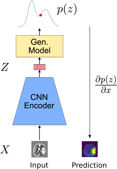
Figure 3: Visualization of the testing/ prediction phase of the model. The anomaly score in image space (anomaly heatmap) is calculated as the derivative of the predicted likelihood with respect to the input image.

Appendix D Experiment Details

General details regarding the experiments is given below and in Tab. 10 the design of the Deep-Convolutional Encoder and Decoder is shown.

• Implementation: Pytorch and Pytorch Lightining.

• Hardware for Training: Single Nvidia GPUs with 12Gb VRAM (Titan XP, 2080Ti).

• Training times: SimCLR $\sim 12$h, GMM $\sim 1$m, RealNVP $\sim 30$m, VAE $\sim 24$h.

• Data augmentations implemented using batchgenerators:

  • SimCLR: random mirroring, random cropping, random scaling, random multiplicative brightness, additive gaussian noise

  • VAE: random scaling, random mirroring, rotations, multiplicative brightness, additive gaussian noise

DC-Encoder	DC-Decoder
Input $x$	Input $z$
4 x 4 Convnf Stride 2, BN, ReLU	4 x 4 Trans-Conv16xnf Stride 1, BN, ReLU
4 x 4 Conv2xnf Stride 2, BN, ReLU	4 x 4 Trans-Conv8xnf Stride 2 Padding 1, BN, ReLU
4 x 4 Conv4xnf Stride 2, BN, ReLU	4 x 4 Trans-Conv4xnf Stride 2 Padding 1, BN, ReLU
4 x 4 Conv8xnf Stride 2. BN, ReLU	4 x 4 Trans-Conv2xnv Stride 2 Padding 1, BN, ReLU
4 x 4 Conv16xnf Stride 2, BN, ReLU	4 x 4 Trans-Convnf Stride 2 Padding 1, BN, ReLU
4 x 4 Convnz Stride 2	4 x 4 Trans-Convnc Stride 2 Padding 1, Sigmoid
Output $z$	Output $\hat{x}$

Table 10: Deep Convolutional Architecture, nf and nz are the hyperparameters for the architecture and bottleneck width. All experiments shown were conducted with nz=512 and nf=64. In the case of VAE and ceVAE nz$=512\cdot 2$ (BN: Batch Normalization)

Gaussian Mixture Models

The Gaussian Mixture Models were implemented in Pytorch to enable fast fits and backpropagation of the NLL.

Normalizing Flow

• Architecture: We used the 8 consecutive flows of the Real NVP Architecture without splitting. Since the Model operates on the representations $z$ (dim=512), we use Linear layers inside the coupling blocks parametrized by $c_{\mathrm{block}}$=512 and $c_{\mathrm{out}}=c_{\mathrm{in}}=256$.

  • Flow:

    1. Coupling Block (Linear($c_{\mathrm{in}}$, $c_{\mathrm{block}}$), ReLU, Linear($c_{\mathrm{block}},c_{\mathrm{out}}))$

    2. Random Permutation of Dimensions

• Training Scheme:

  • We added additional Gaussian noise ($\sigma=$1E-3) to our samples as preprocessing

  • Optimization Parameters: 60 epochs on the representations of the HCP training set with Adam Optimizer and the following parameters: learning rate 1E-3, weight decay 1E-4, gradient clipping (grad_clip_val=5 and additionally the learning rate is divided by 10 every 20 epochs

  • We chose the model for later evaluation based on the smallest loss on the HCP validation set.

Appendix E Data Description

Additional to the statistical information about the dataset for evaulation in Sec. 4, we also show visual examples in Fig. 4.

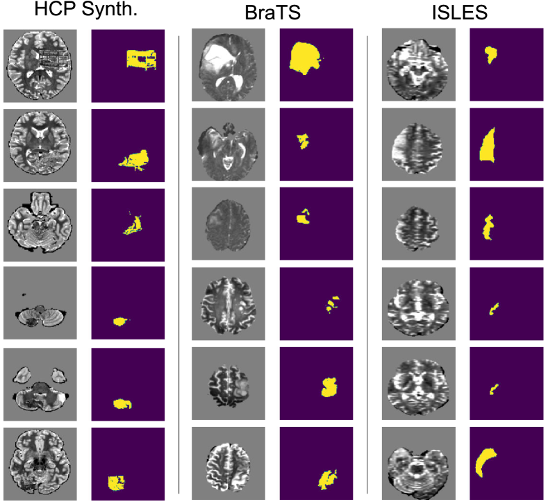
Figure 4: Visual examples of the anomalies present in our synthetically created in-house dataset HCP Synth., BraTS as well as ISLES. Shown are 6 exemplary images for each dataset with their corresponding reference annotations. Please note, that while for BraTS and ISLES, the anomaly primarily differs from the normal tissue by intensity (which can be seen as a bright area), for the HCP Synth. dataset the anomalies also differ by texture and hence might present a better use-case for anomaly detection methods [12].

References

- [1] Andrzej Żytkowski et al. “Anatomical normality and variability: Historical perspective and methodological considerations” In Translational Research in Anatomy 23, 2021, pp. 100105 DOI: https://doi.org/10.1016/j.tria.2020.100105
- [2] Ravi Aggarwal et al. “Diagnostic accuracy of deep learning in medical imaging: A systematic review and meta-analysis” In NPJ digital medicine 4.1 Nature Publishing Group, 2021, pp. 1–23
- [3] Scott Mayer McKinney et al. “International Evaluation of an AI System for Breast Cancer Screening” In Nature 577.7788, 2020, pp. 89–94 DOI: 10.1038/s41586-019-1799-6
- [4] Christopher J. Kelly et al. “Key Challenges for Delivering Clinical Impact with Artificial Intelligence” In BMC Med 17.1, 2019, pp. 195 DOI: 10.1186/s12916-019-1426-2
- [5] “Dacie and Lewis Practical Haematology” Philadelphia, Pa.: Elsevier, 2017
- [6] Christoph Baur et al. “Autoencoders for unsupervised anomaly segmentation in brain MR images: A comparative study” In Medical Image Analysis 69, 2021, pp. 101952 DOI: 10.1016/j.media.2020.101952
- [7] Xiaoran Chen, Suhang You, Kerem Can Tezcan and Ender Konukoglu “Unsupervised Lesion Detection via Image Restoration with a Normative Prior” In Medical Image Analysis 64, 2020, pp. 101713 DOI: 10.1016/j.media.2020.101713
- [8] Thomas Schlegl et al. “F-AnoGAN: Fast Unsupervised Anomaly Detection with Generative Adversarial Networks” In Medical Image Analysis 54, 2019, pp. 30–44 DOI: 10.1016/j.media.2019.01.010
- [9] Eric Nalisnick et al. “Do Deep Generative Models Know What They Don’t Know?” In arXiv:1810.09136 [cs, stat], 2019 arXiv:1810.09136 [cs, stat]
- [10] Jie Ren et al. “Likelihood Ratios for Out-of-Distribution Detection” In arXiv:1906.02845 [cs, stat], 2019 arXiv:1906.02845 [cs, stat]
- [11] Zhisheng Xiao, Qing Yan and Yali Amit “Likelihood Regret: An Out-of-Distribution Detection Score For Variational Auto-Encoder” In arXiv:2003.02977 [cs, stat], 2020 arXiv:2003.02977 [cs, stat]
- [12] Felix Meissen, Georgios Kaissis and Daniel Rueckert “Challenging Current Semi-Supervised Anomaly Segmentation Methods for Brain MRI”, 2021 arXiv:2109.06023 [eess.IV]
- [13] David Zimmerer et al. “Context-Encoding Variational Autoencoder for Unsupervised Anomaly Detection” In arXiv:1812.05941 [cs, stat], 2018 arXiv:1812.05941 [cs, stat]
- [14] Ting Chen, Simon Kornblith, Mohammad Norouzi and Geoffrey Hinton “A Simple Framework for Contrastive Learning of Visual Representations” In arXiv:2002.05709 [cs, stat], 2020 arXiv:2002.05709 [cs, stat]
- [15] David Zimmerer et al. “Unsupervised Anomaly Localization Using Variational Auto-Encoders” In arXiv:1907.02796 [cs, eess, stat], 2019 arXiv:1907.02796 [cs, eess, stat]
- [16] Christoph Baur, Benedikt Wiestler, Shadi Albarqouni and Nassir Navab “Deep autoencoding models for unsupervised anomaly segmentation in brain MR images” In International MICCAI brainlesion workshop, 2018, pp. 161–169 Springer
- [17] Walter Hugo Lopez Pinaya et al. “Unsupervised Brain Anomaly Detection and Segmentation with Transformers” In arXiv:2102.11650 [cs, eess, q-bio], 2021 arXiv:2102.11650 [cs, eess, q-bio]
- [18] Sergio Naval Marimont and Giacomo Tarroni “Anomaly detection through latent space restoration using vector quantized variational autoencoders” In 2021 IEEE 18th International Symposium on Biomedical Imaging (ISBI), 2021, pp. 1764–1767 IEEE
- [19] Eric Nalisnick, Akihiro Matsukawa, Yee Whye Teh and Balaji Lakshminarayanan “Detecting Out-of-Distribution Inputs to Deep Generative Models Using Typicality” In arXiv:1906.02994 [cs, stat], 2019 arXiv:1906.02994 [cs, stat]
- [20] Shiyu Liang, Yixuan Li and R. Srikant “Enhancing The Reliability of Out-of-Distribution Image Detection in Neural Networks” In arXiv:1706.02690 [cs, stat], 2020 arXiv:1706.02690 [cs, stat]
- [21] Kimin Lee, Kibok Lee, Honglak Lee and Jinwoo Shin “A Simple Unified Framework for Detecting Out-of-Distribution Samples and Adversarial Attacks” In arXiv:1807.03888 [cs, stat], 2018 arXiv:1807.03888 [cs, stat]
- [22] Jim Winkens et al. “Contrastive Training for Improved Out-of-Distribution Detection” In arXiv:2007.05566 [cs, stat], 2020 arXiv:2007.05566 [cs, stat]
- [23] Hongjie Zhang, Ang Li, Jie Guo and Yanwen Guo “Hybrid Models for Open Set Recognition” In arXiv:2003.12506 [cs], 2020 arXiv:2003.12506 [cs]
- [24] Ian Goodfellow, Yoshua Bengio and Aaron Courville “Deep Learning” http://www.deeplearningbook.org MIT Press, 2016
- [25] Lars Maaløe, Marco Fraccaro, Valentin Liévin and Ole Winther “BIVA: A Very Deep Hierarchy of Latent Variables for Generative Modeling” In arXiv:1902.02102 [cs, stat], 2019 arXiv:1902.02102 [cs, stat]
- [26] Ting Chen et al. “Big Self-Supervised Models Are Strong Semi-Supervised Learners” In arXiv:2006.10029 [cs, stat], 2020 arXiv:2006.10029 [cs, stat]
- [27] Jean-Bastien Grill et al. “Bootstrap Your Own Latent: A New Approach to Self-Supervised Learning” In arXiv:2006.07733 [cs, stat], 2020 arXiv:2006.07733 [cs, stat]
- [28] A.. Dempster, N.. Laird and D.. Rubin “Maximum Likelihood from Incomplete Data Via the EM Algorithm” In Journal of the Royal Statistical Society: Series B (Methodological) 39.1, 1977, pp. 1–22 DOI: 10.1111/j.2517-6161.1977.tb01600.x
- [29] Laurent Dinh, Jascha Sohl-Dickstein and Samy Bengio “Density Estimation Using Real NVP” In arXiv:1605.08803 [cs, stat], 2017 arXiv:1605.08803 [cs, stat]
- [30] D.C. Van Essen et al. “The Human Connectome Project: A Data Acquisition Perspective” In NeuroImage 62.4, 2012, pp. 2222–2231 DOI: 10.1016/j.neuroimage.2012.02.018
- [31] David Zimmerer et al. “Medical Out-of-Distribution Analysis Challenge” Zenodo, 2020 DOI: 10.5281/ZENODO.3784230
- [32] Oskar Maier et al. “ISLES 2015 - A Public Evaluation Benchmark for Ischemic Stroke Lesion Segmentation from Multispectral MRI” In Medical Image Analysis 35, 2017, pp. 250–269 DOI: 10.1016/j.media.2016.07.009
- [33] Spyridon Bakas et al. “Advancing The Cancer Genome Atlas Glioma MRI Collections with Expert Segmentation Labels and Radiomic Features” In Sci Data 4.1, 2017, pp. 170117 DOI: 10.1038/sdata.2017.117
- [34] Alec Radford, Luke Metz and Soumith Chintala “Unsupervised Representation Learning with Deep Convolutional Generative Adversarial Networks” In arXiv:1511.06434 [cs], 2016 arXiv:1511.06434 [cs]
- [35] Ilya Loshchilov and Frank Hutter “SGDR: Stochastic Gradient Descent with Warm Restarts” In arXiv:1608.03983 [cs, math], 2017 arXiv:1608.03983 [cs, math]
- [36] Chun-Liang Li, Kihyuk Sohn, Jinsung Yoon and Tomas Pfister “CutPaste: Self-Supervised Learning for Anomaly Detection and Localization” In 2021 IEEE/CVF Conference on Computer Vision and Pattern Recognition (CVPR), 2021, pp. 9659–9669 DOI: 10.1109/CVPR46437.2021.00954
- [37] Kaiming He et al. “Masked Autoencoders Are Scalable Vision Learners”, 2021 arXiv:2111.06377 [cs.CV]