A tensor bidiagonalization method for higher-order singular value decomposition with applications

A. El Hachimi22footnotemark: 2 Laboratory MSDA, Mohammed VI Polytechnic University, Green City, Morocco.    K. Jbilou11footnotemark: 1 Université du Littoral Cote d’Opale, LMPA, 50 rue F. Buisson, 62228 Calais-Cedex, France    A. Ratnani11footnotemark: 1    L. Reichel Department of Mathematical Sciences, Kent State University, Kent, OH 44242, USA.
Abstract

The need to know a few singular triplets associated with the largest singular values of third-order tensors arises in data compression and extraction. This paper describes a new method for their computation using the t-product. Methods for determining a couple of singular triplets associated with the smallest singular values also are presented. The proposed methods generalize available restarted Lanczos bidiagonalization methods for computing a few of the largest or smallest singular triplets of a matrix. The methods of this paper use Ritz and harmonic Ritz lateral slices to determine accurate approximations of the largest and smallest singular triplets, respectively. Computed examples show applications to data compression and face recognition.

keywords:
tensors, t-product, partial tensor bidiagonalization, restarted tensor bidiagonalization, singular value decomposition, face recognition.

1 Introduction

The last 20 years has seen an immense growth of the amount of data that is collected for analysis, but it is a challenging problem to extract useful information from available data. This difficulty arises, e.g., in machine learning, data mining, and deep learning; see, e.g., Arnold et al. [1]. The extraction of useful information from data that is represented by a matrix often is facilitated by the singular value decomposition of the matrix. Typically, only a few of the largest singular triplets, i.e., the largest singular values and associated right and left singular vectors, are required to extract useful information from the matrix. A restarted Lanczos bidiagonalization method for computing accurate approximations of these singular triplets is described in [5], and R code written by Bryan W. Lewis is available at [6].

In many recent applications the given data are represented by a multidimensional array. These arrays, known as tensors, are natural generalizations of matrices. Several approaches to define tensor-tensor products and tensor-matrix products are described in the literature, including the n𝑛n-mode product [9, 25], the t-product [22, 31], and the c-product [21, 30]. Generalizations of the singular value decomposition (SVD) to tensors are described in [25] using the n𝑛n-mode product (the so-called HOSVD), and in [21, 22] using the tensor c-product and t-product. The need to compute the SVD or a partial SVD of a tensor arises in a variety of applications, including image restoration, tensor completion [10], robust tensor principal component analysis [13], tensor compression [3], and recognition of color faces [17, 18]. These applications require knowledge of the largest singular values and associated lateral tensor singular slices.

It is the purpose of the this paper to introduce a new restarted tensor Lanczos bidiagonalization method for third-order tensors using the t-product for approximating a few of the largest singular values and associated lateral tensor singular slices. This method generalizes the approach described in [5] from matrices to tensors. We remark that the Lanczos bidiagonalization method (also known as the Golub-Kahan bidiagonalization method) for third-order tensors using the t-product has been described in [15, 16, 22, 32]; however, this bidiagonalization method differs from the one of the present paper.

In [5] the authors also describe a restarted Lanczos bidiagonalization method for the computation of a few of the smallest singular values and associated singular vectors of a large matrix by determining harmonic Ritz values is presented. This paper presents an analogous scheme for third-order tensors.

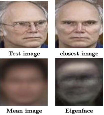
The organization of this paper is as follows. Section 2 recalls some properties of the t-product and Section 3 reviews tensor Lanczos bidiagonalization of third-order tensors using the t-product. Restarted tensor Lanczos bidiagonalization methods are presented for the approximation of a few of the largest singular values and associated lateral tensor singular slices by computing lateral tensor Ritz slices, as well as for approximating a few of the smallest singular values and associated lateral tensor singular slices by evaluating harmonic lateral tensor Ritz slices. Section 4 discusses multidimensional principal component analysis using a partial tensor HOSVD with application to face recognition, and Section 5 presents a few computed examples. Concluding remarks and possible extensions can be found in Section 6.

2 The tensor t-product

This section reviews results by Kilmer et al. [22, 23] and uses notation employed there and by Kolda and Bader [25]. A third-order tensor is an array 𝒜=[aijk]×p×n𝒜delimited-[]subscript𝑎𝑖𝑗𝑘superscript𝑝𝑛\mathscr{A}=[a_{ijk}]\in\mathbb{R}^{\ell\times p\times n}. Matrices and vectors are tensors of order two and one, respectively. A slice or frame of a third-order tensor 𝒜𝒜\mathscr{A} is a section obtained by fixing any one of the three indices. Using MATLAB notation, 𝒜(i,:,:)𝒜𝑖::\mathscr{A}(i,:,:), 𝒜(:,j,:)𝒜:𝑗:\mathscr{A}(:,j,:), and 𝒜(:,:,k)𝒜::𝑘\mathscr{A}(:,:,k) denote the i𝑖ith horizontal, the j𝑗jth lateral, and the k𝑘kth frontal slices of 𝒜𝒜\mathscr{A}, respectively. The lateral slice 𝒜(:,j,:)𝒜:𝑗:\mathscr{A}(:,j,:) also is denoted by 𝒜jsubscript𝒜𝑗\vec{\mathscr{A}}_{j}, and the frontal slice 𝒜(:,:,k)𝒜::𝑘\mathscr{A}(:,:,k) is an ×p𝑝\ell\times p matrix that is sometimes denoted by 𝒜(k)superscript𝒜𝑘\mathscr{A}^{(k)}. A fiber of a third order tensor 𝒜𝒜\mathscr{A} is defined by fixing any two of the three indices. The fiber 𝒜(i,j,:)𝒜𝑖𝑗:\mathscr{A}(i,j,:) is called a tube of 𝒜𝒜\mathscr{A}. We will use capital calligraphic letters 𝒜𝒜\mathscr{A} to denote third-order tensors, capital letters A𝐴A to identify matrices, bold face lower case letters 𝒂𝒂\bm{a} to denote tubes, and lower case letters a𝑎a stand for scalars. Further, 𝕂n×p=×p×nsubscriptsuperscript𝕂𝑝𝑛superscript𝑝𝑛\mathbb{K}^{\ell\times p}_{n}=\mathbb{R}^{\ell\times p\times n} denotes the space of third-order tensors of size ×p×n𝑝𝑛\ell\times p\times n, 𝕂n=×1×nsubscriptsuperscript𝕂𝑛superscript1𝑛\mathbb{K}^{\ell}_{n}=\mathbb{R}^{\ell\times 1\times n} stands for the space of lateral slices of size ×n𝑛\ell\times n, and 𝕂n=1×1×nsubscript𝕂𝑛superscript11𝑛\mathbb{K}_{n}=\mathbb{R}^{1\times 1\times n} denotes the space of tubes with n𝑛n entries. For a third-order tensor 𝒜𝕂n×p𝒜subscriptsuperscript𝕂𝑝𝑛\mathscr{A}\in\mathbb{K}^{\ell\times p}_{n} with frontal slices 𝒜(i)superscript𝒜𝑖\mathscr{A}^{(i)}, i=1,,n𝑖1𝑛i=1,\ldots,n, we define:

  • The block circulant matrix associated with 𝒜𝒜\mathscr{A}:

    𝚋𝚌𝚒𝚛𝚌(𝒜)=[𝒜(1)𝒜(n)𝒜(2)𝒜(2)𝒜(1)𝒜(3)𝒜(n)𝒜(n1)𝒜(1)]𝕂n×pn.𝚋𝚌𝚒𝚛𝚌𝒜matrixsuperscript𝒜1superscript𝒜𝑛superscript𝒜2superscript𝒜2superscript𝒜1superscript𝒜3superscript𝒜𝑛superscript𝒜𝑛1superscript𝒜1superscript𝕂𝑛𝑝𝑛{\tt bcirc}(\mathscr{A})=\begin{bmatrix}\mathscr{A}^{(1)}&\mathscr{A}^{(n)}&\ldots&\mathscr{A}^{(2)}\\ \mathscr{A}^{(2)}&\mathscr{A}^{(1)}&\ldots&\mathscr{A}^{(3)}\\ \vdots&\ddots&\ddots&\vdots\\ \mathscr{A}^{(n)}&\mathscr{A}^{(n-1)}&\ldots&\mathscr{A}^{(1)}\\ \end{bmatrix}\in\mathbb{K}^{\ell n\times pn}. (1)
  • The operator 𝚞𝚗𝚏𝚘𝚕𝚍𝚞𝚗𝚏𝚘𝚕𝚍{\tt unfold} applied to 𝒜𝒜{\mathscr{A}} gives the matrix made up of its frontal slices,

    𝚞𝚗𝚏𝚘𝚕𝚍(𝒜)=[𝒜(1)𝒜(2)𝒜(n)]𝕂n×p.𝚞𝚗𝚏𝚘𝚕𝚍𝒜matrixsuperscript𝒜1superscript𝒜2superscript𝒜𝑛superscript𝕂𝑛𝑝{\tt unfold}(\mathscr{A})=\begin{bmatrix}\mathscr{A}^{(1)}\\ \mathscr{A}^{(2)}\\ \vdots\\ \mathscr{A}^{(n)}\end{bmatrix}\in\mathbb{K}^{\ell n\times p}.

    We also will need the inverse operator 𝚏𝚘𝚕𝚍𝚏𝚘𝚕𝚍{\tt fold} such that 𝚏𝚘𝚕𝚍(𝚞𝚗𝚏𝚘𝚕𝚍(𝒜))=𝒜𝚏𝚘𝚕𝚍𝚞𝚗𝚏𝚘𝚕𝚍𝒜𝒜{\tt fold}\left(\tt unfold\left(\mathscr{A}\right)\right)=\mathscr{A}.

  • The block diagonal matrix associated with 𝒜𝒜\mathscr{A} is defined as

    𝚋𝚍𝚒𝚊𝚐(𝒜)=[𝒜(1)𝒜(2)𝒜(n)]𝕂n×pn.𝚋𝚍𝚒𝚊𝚐𝒜matrixsuperscript𝒜1missing-subexpressionmissing-subexpressionmissing-subexpressionmissing-subexpressionsuperscript𝒜2missing-subexpressionmissing-subexpressionmissing-subexpressionmissing-subexpressionmissing-subexpressionmissing-subexpressionmissing-subexpressionmissing-subexpressionsuperscript𝒜𝑛superscript𝕂𝑛𝑝𝑛{\tt bdiag}\left(\mathscr{A}\right)=\begin{bmatrix}\mathscr{A}^{(1)}&&&\\ &\mathscr{A}^{(2)}&&\\ &&\ddots&\\ &&&\mathscr{A}^{(n)}\end{bmatrix}\in\mathbb{K}^{\ell n\times pn}.
Definition 1.

([23]) Let 𝒜𝕂n×q𝒜subscriptsuperscript𝕂𝑞𝑛\mathscr{A}\in\mathbb{K}^{\ell\times q}_{n} and 𝕂nq×psubscriptsuperscript𝕂𝑞𝑝𝑛\mathscr{B}\in\mathbb{K}^{q\times p}_{n} be third-order tensors. The t-product of 𝒜𝒜\mathscr{A} and \mathscr{B} is defined by

𝒜:=𝚏𝚘𝚕𝚍(𝚋𝚌𝚒𝚛𝚌(𝒜)𝚞𝚗𝚏𝚘𝚕𝚍())𝕂n×p.assign𝒜𝚏𝚘𝚕𝚍𝚋𝚌𝚒𝚛𝚌𝒜𝚞𝚗𝚏𝚘𝚕𝚍subscriptsuperscript𝕂𝑝𝑛\mathscr{A}\star\mathscr{B}:={\tt fold}\left({\tt bcirc}(\mathscr{A})\,{\tt unfold}(\mathscr{B})\right)\in\mathbb{K}^{\ell\times p}_{n}.

The block circulant matrix (1) can be block-diagonalized by using the discrete Fourier transform (DFT) as follows:

𝚋𝚌𝚒𝚛𝚌(𝒜)=(FnHI)𝚋𝚍𝚒𝚊𝚐(𝒜^)(FnIp),𝚋𝚌𝚒𝚛𝚌𝒜tensor-productsuperscriptsubscript𝐹𝑛𝐻subscript𝐼𝚋𝚍𝚒𝚊𝚐^𝒜tensor-productsubscript𝐹𝑛subscript𝐼𝑝{\tt bcirc}(\mathscr{A})=\left(F_{n}^{H}\otimes I_{\ell}\right){\tt bdiag}(\widehat{\mathscr{A}})\left(F_{n}\otimes I_{p}\right),

where Fnn×nsubscript𝐹𝑛superscript𝑛𝑛F_{n}\in\mathbb{C}^{n\times n} is the discrete Fourier matrix, FnHsuperscriptsubscript𝐹𝑛𝐻F_{n}^{H} denotes its conjugate transpose, 𝒜^^𝒜\widehat{\mathscr{A}} stands for the Fourier transform of 𝒜𝒜\mathscr{A} along each tube, I×subscript𝐼superscriptI_{\ell}\in\mathbb{R}^{\ell\times\ell} denotes the identity matrix, and tensor-product\otimes is the Kronecker product. The matrix 𝒜^^𝒜\widehat{\mathscr{A}} can be computed with the fast Fourier transform (FFT) algorithm; see [23] for details. Using MATLAB notations, we have

𝒜^=𝚏𝚏𝚝(𝒜,[],3).^𝒜𝚏𝚏𝚝𝒜3\widehat{\mathscr{A}}={\tt fft}(\mathscr{A},[\,],3).

The inverse operation can be evaluated in MATLAB with the command

𝒜=𝚒𝚏𝚏𝚝(𝒜^,[],3).𝒜𝚒𝚏𝚏𝚝^𝒜3\mathscr{A}={\tt ifft}(\widehat{\mathscr{A}},[\,],3).

Hence, the t-product 𝒞=𝒜𝒞𝒜\mathscr{C}=\mathscr{A}\star\mathscr{B} can be evaluated as

𝒞^(i)=𝒜^(i)^(i),i=1,2,,n,formulae-sequencesuperscript^𝒞𝑖superscript^𝒜𝑖superscript^𝑖𝑖12𝑛\widehat{\mathscr{C}}^{(i)}=\widehat{\mathscr{A}}^{(i)}\widehat{\mathscr{B}}^{(i)},\qquad i=1,2,\ldots,n, (2)

where 𝒜^(i)superscript^𝒜𝑖\widehat{\mathscr{A}}^{(i)}, ^(i)superscript^𝑖\widehat{\mathscr{B}}^{(i)}, and 𝒞^(i)superscript^𝒞𝑖\widehat{\mathscr{C}}^{(i)} are the i𝑖ith frontal slices of the tensors 𝒜^^𝒜\widehat{\mathscr{A}}, ^^\widehat{\mathscr{B}}, and 𝒞^^𝒞\widehat{\mathscr{C}}, respectively.

As already pointed out by Kilmer et al. [22], one can use symmetry properties of the DFT when applied to real data to reduce the computational effort when evaluating the t-product with the FFT. This is described by the following result, which can be found, e.g., in [33].

Lemma 1.

Given a real vector vn𝑣superscript𝑛v\in\mathbb{R}^{n}, the associated DFT vector v^=Fnv^𝑣subscript𝐹𝑛𝑣\widehat{v}=F_{n}v satisfies

v^1,𝚌𝚘𝚗𝚓(v^i)=v^ni+2,i=2,3,,[n+12],formulae-sequencesubscript^𝑣1formulae-sequence𝚌𝚘𝚗𝚓subscript^𝑣𝑖subscript^𝑣𝑛𝑖2𝑖23delimited-[]𝑛12\widehat{v}_{1}\in\mathbb{R},\quad{\tt conj}\left(\widehat{v}_{i}\right)=\widehat{v}_{n-i+2},\quad i=2,3,\ldots,\left[\dfrac{n+1}{2}\right],

where 𝚌𝚘𝚗𝚓𝚌𝚘𝚗𝚓{\tt conj} denotes the complex conjugation operator and [n+12]delimited-[]𝑛12\left[\dfrac{n+1}{2}\right] denotes the integer part of n+12𝑛12\dfrac{n+1}{2}.

It follows that for a third-order tensor 𝒜𝕂n×p𝒜subscriptsuperscript𝕂𝑝𝑛\mathscr{A}\in\mathbb{K}^{\ell\times p}_{n}, we have

𝒜^(1)×p,𝚌𝚘𝚗𝚓(𝒜^(i))=𝒜^(ni+2),i=2,3,,[n+12].formulae-sequencesuperscript^𝒜1superscript𝑝formulae-sequence𝚌𝚘𝚗𝚓superscript^𝒜𝑖superscript^𝒜𝑛𝑖2𝑖23delimited-[]𝑛12\widehat{\mathscr{A}}^{(1)}\in\mathbb{R}^{\ell\times p},\quad{\tt conj}\left(\widehat{\mathscr{A}}^{(i)}\right)=\widehat{\mathscr{A}}^{(n-i+2)},\quad i=2,3,\ldots,\left[\dfrac{n+1}{2}\right].

This shows that the t-product of two third-order tensors can be determined by evaluating just about half the number of products involved in (2). Algorithm 1 describes the computations.

Algorithm 1 t-product of third-order tensors.

Input: 𝒜𝕂n×q𝒜subscriptsuperscript𝕂𝑞𝑛\mathscr{A}\in\mathbb{K}^{\ell\times q}_{n}, 𝕂nq×psubscriptsuperscript𝕂𝑞𝑝𝑛\mathscr{B}\in\mathbb{K}^{q\times p}_{n}.
Output: 𝒞:=𝒜𝕂n×passign𝒞𝒜subscriptsuperscript𝕂𝑝𝑛\mathscr{C}:=\mathscr{A}\star\mathscr{B}\in\mathbb{K}^{\ell\times p}_{n}.

1:  Compute 𝒜^=𝚏𝚏𝚝(𝒜,[],3)^𝒜𝚏𝚏𝚝𝒜3\widehat{\mathscr{A}}={\tt fft}(\mathscr{A},[\,],3), ^=𝚏𝚏𝚝(,[],3)^𝚏𝚏𝚝3\widehat{\mathscr{B}}={\tt fft}(\mathscr{B},[\,],3).
2:  for i=1,,[n+12]𝑖1delimited-[]𝑛12i=1,\ldots,\left[\dfrac{n+1}{2}\right] do
3:     𝒞^(i)=𝒜^(i)^(i)superscript^𝒞𝑖superscript^𝒜𝑖superscript^𝑖\phantom{000}\widehat{\mathscr{C}}^{(i)}=\widehat{\mathscr{A}}^{(i)}\widehat{\mathscr{B}}^{(i)}.
4:  end for
5:  for i=[n+12]+1,,n𝑖delimited-[]𝑛121𝑛i=\left[\dfrac{n+1}{2}\right]+1,\ldots,n do
6:     𝒞^(i)=𝚌𝚘𝚗𝚓(𝒞^(ni+2))superscript^𝒞𝑖𝚌𝚘𝚗𝚓superscript^𝒞𝑛𝑖2\phantom{000}\widehat{\mathscr{C}}^{(i)}={\tt conj}\left(\widehat{\mathscr{C}}^{(n-i+2)}\right).
7:  end for
8:  𝒞=𝚒𝚏𝚏𝚝(𝒞^,[],3)𝒞𝚒𝚏𝚏𝚝^𝒞3\mathscr{C}={\tt ifft}\left(\widehat{\mathscr{C}},[\,],3\right).

The following definition is concerned with the t-product of a third-order tensor and a tube.

Definition 2.

Let 𝒜𝕂n×p𝒜subscriptsuperscript𝕂𝑝𝑛\mathscr{A}\in\mathbb{K}^{\ell\times p}_{n} and 𝐛𝕂n𝐛subscript𝕂𝑛\bm{b}\in\mathbb{K}_{n}. Then 𝒞:=𝒜𝐛𝕂n×passign𝒞𝒜𝐛subscriptsuperscript𝕂𝑝𝑛\mathscr{C}:=\mathscr{A}\star\bm{b}\in\mathbb{K}^{\ell\times p}_{n} is obtained by applying the inverse DFT along each tube of 𝒞^^𝒞\widehat{\mathscr{C}}, where each frontal slice is determined by the standard matrix product between each frame of 𝒜^^𝒜\widehat{\mathscr{A}} and 𝐛^^𝐛\widehat{\bm{b}}, i.e.,

𝒞^(i)=𝒜^(i)𝒃^(i)=𝒃^(i)𝒜^(i),i=1,2,,n.formulae-sequencesuperscript^𝒞𝑖superscript^𝒜𝑖superscript^𝒃𝑖superscript^𝒃𝑖superscript^𝒜𝑖𝑖12𝑛\widehat{\mathscr{C}}^{(i)}=\widehat{\mathscr{A}}^{(i)}\widehat{\bm{b}}^{(i)}={\color[rgb]{0,0,0}\definecolor[named]{pgfstrokecolor}{rgb}{0,0,0}\pgfsys@color@gray@stroke{0}\pgfsys@color@gray@fill{0}\widehat{\bm{b}}^{(i)}\widehat{\mathscr{A}}^{(i)}},\quad i=1,2,\ldots,n.

A third-order tensor 𝒜𝕂n×p𝒜subscriptsuperscript𝕂𝑝𝑛\mathscr{A}\in\mathbb{K}^{\ell\times p}_{n} can be written as

𝒜=[𝒜1,𝒜2,,𝒜p],𝒜subscript𝒜1subscript𝒜2subscript𝒜𝑝\mathscr{A}=\left[\vec{\mathscr{A}}_{1},\vec{\mathscr{A}}_{2},\ldots,\vec{\mathscr{A}}_{p}\right],

thus, for the tensors 𝒜𝕂n×q𝒜subscriptsuperscript𝕂𝑞𝑛\mathscr{A}\in\mathbb{K}^{\ell\times q}_{n} and 𝕂nq×psubscriptsuperscript𝕂𝑞𝑝𝑛\mathscr{B}\in\mathbb{K}^{q\times p}_{n}, the t-product 𝒜𝒜\mathscr{A}\star\mathscr{B} can be expressed as

𝒜=[𝒜1,𝒜2,,𝒜p],𝒜𝒜subscript1𝒜subscript2𝒜subscript𝑝\mathscr{A}\star\mathscr{B}=\left[\mathscr{A}\star\vec{\mathscr{B}}_{1},\mathscr{A}\star\vec{\mathscr{B}}_{2},\ldots,\mathscr{A}\star\vec{\mathscr{B}}_{p}\right],

where

𝒜i=(𝒜)i,i=1,2,,p.formulae-sequence𝒜subscript𝑖subscript𝒜𝑖𝑖12𝑝\mathscr{A}\star\overrightarrow{\mathscr{B}}_{i}=\overrightarrow{\left(\mathscr{A}\star\mathscr{B}\right)}_{i},\quad i=1,2,\ldots,p.

The Frobenius norm of a third-order tensor 𝒜𝕂n×p𝒜subscriptsuperscript𝕂𝑝𝑛\mathscr{A}\in\mathbb{K}^{\ell\times p}_{n} is given by

𝒜F:=i1,i2,i3=1,p,nai1,i2,i32,assignsubscriptnorm𝒜𝐹superscriptsubscriptsubscript𝑖1subscript𝑖2subscript𝑖31𝑝𝑛superscriptsubscript𝑎subscript𝑖1subscript𝑖2subscript𝑖32\left\|\mathscr{A}\right\|_{F}:=\sqrt{\sum_{i_{1},i_{2},i_{3}=1}^{\ell,p,n}a_{i_{1},i_{2},i_{3}}^{2}},

and the inner product of two third-order tensors of the same size 𝒜,𝕂n×p𝒜subscriptsuperscript𝕂𝑝𝑛\mathscr{A},\mathscr{B}\in\mathbb{K}^{\ell\times p}_{n} is defined as

𝒜,:=i1,i2,i3=1,p,nai1,i2,i3bi1,i2,i3.assign𝒜superscriptsubscriptsubscript𝑖1subscript𝑖2subscript𝑖31𝑝𝑛subscript𝑎subscript𝑖1subscript𝑖2subscript𝑖3subscript𝑏subscript𝑖1subscript𝑖2subscript𝑖3\langle\mathscr{A},\mathscr{B}\rangle:=\sum_{i_{1},i_{2},i_{3}=1}^{\ell,p,n}a_{i_{1},i_{2},i_{3}}b_{i_{1},i_{2},i_{3}}.

We have the relations

𝒜F=1n𝒜^F,𝒜,=1n𝒜^,^.formulae-sequencesubscriptnorm𝒜𝐹1𝑛subscriptnorm^𝒜𝐹𝒜1𝑛^𝒜^\left\|\mathscr{A}\right\|_{F}=\dfrac{1}{\sqrt{n}}\left\|\widehat{\mathscr{A}}\right\|_{F},\qquad\langle\mathscr{A},\mathscr{B}\rangle=\dfrac{1}{n}\langle\widehat{\mathscr{A}},\widehat{\mathscr{B}}\rangle.

We recall for later use the definitions of some special tensors and operations:

  • The identity tensor 𝕂n×subscriptsubscriptsuperscript𝕂𝑛\mathscr{I}_{\ell}\in\mathbb{K}^{\ell\times\ell}_{n} is the tensor whose first frontal slice is the identity matrix and all other slices have zero entries only.

  • The transpose of a real third-order tensor, 𝒜𝕂n×p𝒜subscriptsuperscript𝕂𝑝𝑛\mathscr{A}\in\mathbb{K}^{\ell\times p}_{n}, denoted by 𝒜H𝕂np×superscript𝒜𝐻subscriptsuperscript𝕂𝑝𝑛\mathscr{A}^{H}\in\mathbb{K}^{p\times\ell}_{n}, is the tensor obtained by first transposing each one of the frontal slices of 𝒜𝒜\mathscr{A}, and then reversing the order of the transposed frontal slices 222 through n𝑛n; see [23]. Let the third-order tensors 𝒜𝒜{\mathscr{A}} and \mathscr{B} be such that the products 𝒜𝒜{\mathscr{A}}\star\mathscr{B} and H𝒜Hsuperscript𝐻superscript𝒜𝐻\mathscr{B}^{H}\star\mathscr{A}^{H} are defined. Then, similarly to the matrix transpose, the tensor transpose satisfies (𝒜)H=H𝒜Hsuperscript𝒜𝐻superscript𝐻superscript𝒜𝐻({\mathscr{A}}\star\mathscr{B})^{H}=\mathscr{B}^{H}\star\mathscr{A}^{H}.

  • A tensor 𝒬𝕂n×𝒬subscriptsuperscript𝕂𝑛\mathscr{Q}\in\mathbb{K}^{\ell\times\ell}_{n} is said to be orthogonal if and only if

    𝒬H𝒬=𝒬𝒬H=.superscript𝒬𝐻𝒬𝒬superscript𝒬𝐻subscript\mathscr{Q}^{H}\star\mathscr{Q}=\mathscr{Q}\star\mathscr{Q}^{H}=\mathscr{I}_{\ell}.
  • A square third-order tensor 𝒜𝕂n×𝒜subscriptsuperscript𝕂𝑛\mathscr{A}\in\mathbb{K}^{\ell\times\ell}_{n} is invertible if there is a third-order tensor 𝕂n×subscriptsuperscript𝕂𝑛\mathscr{B}\in\mathbb{K}^{\ell\times\ell}_{n} such that

    𝒜=,𝒜=.formulae-sequence𝒜subscript𝒜subscript\mathscr{A}\star\mathscr{B}=\mathscr{I}_{\ell},\quad\mathscr{B}\star\mathscr{A}=\mathscr{I}_{\ell}.

    In this case \mathscr{B} is said to be the inverse of 𝒜𝒜\mathscr{A}, and is denoted by 𝒜1superscript𝒜1\mathscr{A}^{-1}.

Definition 3.

([22]) Let 𝒜i𝕂nsubscript𝒜𝑖subscriptsuperscript𝕂𝑛\vec{\mathscr{A}}_{i}\in\mathbb{K}^{\ell}_{n} for i=1,2,,p𝑖12𝑝i=1,2,\ldots,p be lateral slices of the tensor 𝒜𝕂n×p𝒜superscriptsubscript𝕂𝑛𝑝\mathscr{A}\in\mathbb{K}_{n}^{\ell\times p}. A t-linear combination of these slices is defined as

𝒜1𝒃1+𝒜2𝒃2++𝒜p𝒃p,subscript𝒜1subscript𝒃1subscript𝒜2subscript𝒃2subscript𝒜𝑝subscript𝒃𝑝\vec{\mathscr{A}}_{1}\star\bm{b}_{1}+\vec{\mathscr{A}}_{2}\star\bm{b}_{2}+\ldots+\vec{\mathscr{A}}_{p}\star\bm{b}_{p},

where the 𝐛isubscript𝐛𝑖\bm{b}_{i} for i=1,2,,p𝑖12𝑝i=1,2,\ldots,p are tubes in 𝕂nsubscript𝕂𝑛\mathbb{K}_{n}. Moreover,

𝚜𝚙𝚊𝚗{𝒜1,𝒜2,,𝒜p}={i=1p𝒜i𝒃i:𝒃i𝕂n,i=1,2,,p}.{\tt span}\left\{\vec{\mathscr{A}}_{1},\vec{\mathscr{A}}_{2},\ldots,\vec{\mathscr{A}}_{p}\right\}=\left\{\sum_{i=1}^{p}\vec{\mathscr{A}}_{i}\star\bm{b}_{i}:\leavevmode\nobreak\ \leavevmode\nobreak\ \bm{b}_{i}\in\mathbb{K}_{n},\leavevmode\nobreak\ \leavevmode\nobreak\ i=1,2,\ldots,p\right\}.

The tensor singular value decomposition (t-SVD) associated with the t-product, introduced by Kilmer and Martin [23], generalizes the classical SVD of a matrix. It is described in the next theorem.

Theorem 4.

([23]) Let 𝒜𝕂n×p𝒜subscriptsuperscript𝕂𝑝𝑛\mathscr{A}\in\mathbb{K}^{\ell\times p}_{n} be a third-order tensor. Then it can be represented as the t-product of three third-order tensors,

𝒜=𝒰𝒮𝒱H,𝒜𝒰𝒮superscript𝒱𝐻\mathscr{A}=\mathscr{U}\star\mathscr{S}\star\mathscr{V}^{H}, (3)

where 𝒰𝕂n×𝒰subscriptsuperscript𝕂𝑛\mathscr{U}\in\mathbb{K}^{\ell\times\ell}_{n} and 𝒱𝕂np×p𝒱subscriptsuperscript𝕂𝑝𝑝𝑛\mathscr{V}\in\mathbb{K}^{p\times p}_{n} are orthogonal tensors, and 𝒮𝕂n×p𝒮subscriptsuperscript𝕂𝑝𝑛\mathscr{S}\in\mathbb{K}^{\ell\times p}_{n} is an f-diagonal tensor, i.e., each frontal slice of the DFT of 𝒮𝒮\mathscr{S} is a diagonal matrix.

Algorithm 2 summarizes the computation of the t-SVD of a third-order tensor with the aid of the FFT.

Algorithm 2 The t-SVD of a third-order tensor.

Input: 𝒜𝕂n×p𝒜subscriptsuperscript𝕂𝑝𝑛\mathscr{A}\in\mathbb{K}^{\ell\times p}_{n}.
Output: 𝒰𝕂n×,𝒮𝕂n×p,𝒱𝕂np×pformulae-sequence𝒰subscriptsuperscript𝕂𝑛formulae-sequence𝒮subscriptsuperscript𝕂𝑝𝑛𝒱subscriptsuperscript𝕂𝑝𝑝𝑛\mathscr{U}\in\mathbb{K}^{\ell\times\ell}_{n},\;\mathscr{S}\in\mathbb{K}^{\ell\times p}_{n},\;\mathscr{V}\in\mathbb{K}^{p\times p}_{n}.

1:  𝒜^=𝚏𝚏𝚝(𝒜,[],3).^𝒜𝚏𝚏𝚝𝒜3\widehat{\mathscr{A}}={\tt fft}(\mathscr{A},[\,],3).
2:  for i=1,,[n+12]𝑖1delimited-[]𝑛12i=1,\ldots,\left[\dfrac{n+1}{2}\right] do
3:     [𝒰^(i),𝒮^(i),𝒱^(i)]=𝚜𝚟𝚍(𝒜^(i))superscript^𝒰𝑖superscript^𝒮𝑖superscript^𝒱𝑖𝚜𝚟𝚍superscript^𝒜𝑖\phantom{000}[\widehat{\mathscr{U}}^{(i)},\widehat{\mathscr{S}}^{(i)},\widehat{\mathscr{V}}^{(i)}]={\tt svd}(\widehat{\mathscr{A}}^{(i)}).
4:  end for
5:  for i=1,,[n+12]+1𝑖1delimited-[]𝑛121i=1,\ldots,\left[\dfrac{n+1}{2}\right]+1 do
6:     𝒰^(i)=𝚌𝚘𝚗𝚓(𝒰^(ni+2))superscript^𝒰𝑖𝚌𝚘𝚗𝚓superscript^𝒰𝑛𝑖2\phantom{000}\widehat{\mathscr{U}}^{(i)}={\tt conj}\left(\widehat{\mathscr{U}}^{(n-i+2)}\right), 𝒮^(i)=𝚌𝚘𝚗𝚓(𝒮^(ni+2))superscript^𝒮𝑖𝚌𝚘𝚗𝚓superscript^𝒮𝑛𝑖2\widehat{\mathscr{S}}^{(i)}={\tt conj}\left(\widehat{\mathscr{S}}^{(n-i+2)}\right), and 𝒱^(i)=𝚌𝚘𝚗𝚓(𝒱^(ni+2))superscript^𝒱𝑖𝚌𝚘𝚗𝚓superscript^𝒱𝑛𝑖2\widehat{\mathscr{V}}^{(i)}={\tt conj}\left(\widehat{\mathscr{V}}^{(n-i+2)}\right).
7:  end for
8:  Compute 𝒰=𝚒𝚏𝚏𝚝(𝒰^,[],3)𝒰𝚒𝚏𝚏𝚝^𝒰3\mathscr{U}={\tt ifft}(\widehat{\mathscr{U}},[\,],3), 𝒮=𝚒𝚏𝚏𝚝(𝒮^,[],3)𝒮𝚒𝚏𝚏𝚝^𝒮3\mathscr{S}={\tt ifft}(\widehat{\mathscr{S}},[\,],3), and 𝒱=𝚒𝚏𝚏𝚝(𝒱^,[],3)𝒱𝚒𝚏𝚏𝚝^𝒱3\mathscr{V}={\tt ifft}(\widehat{\mathscr{V}},[\,],3).

The factorization (3) can be expressed as

𝒜=𝒰𝒮𝒱H=i=1min{,p}𝒰i𝒔i𝒱iH,𝒜𝒰𝒮superscript𝒱𝐻superscriptsubscript𝑖1𝑝subscript𝒰𝑖subscript𝒔𝑖superscriptsubscript𝒱𝑖𝐻\mathscr{A}=\mathscr{U}\star\mathscr{S}\star\mathscr{V}^{H}=\sum_{i=1}^{\min\{\ell,p\}}\vec{\mathscr{U}}_{i}\star\bm{s}_{i}\star\vec{\mathscr{V}}_{i}^{H},

where the 𝒔i=𝒮(i,i,:)subscript𝒔𝑖𝒮𝑖𝑖:\bm{s}_{i}=\mathscr{S}(i,i,:) are singular tubes, and 𝒰i=𝒰(:,i,:)subscript𝒰𝑖𝒰:𝑖:\vec{\mathscr{U}}_{i}=\mathscr{U}(:,i,:) and 𝒱i=𝒰(:,i,:)subscript𝒱𝑖𝒰:𝑖:\vec{\mathscr{V}}_{i}=\mathscr{U}(:,i,:) are right and left lateral tensor singular slices, respectively, for i=1,2,,min(,p)𝑖12𝑝i=1,2,\ldots,\min(\ell,p). The triplets {𝒔i,𝒰i,𝒱i}i=1:min(,p)subscriptsubscript𝒔𝑖subscript𝒰𝑖subscript𝒱𝑖:𝑖1𝑝\{\bm{s}_{i},\vec{\mathscr{U}}_{i},\vec{\mathscr{V}}_{i}\}_{i=1:\min(\ell,p)} will be referred to as singular triplets of the tensor 𝒜𝒜\mathscr{A}. The singular tubes are ordered so that their norms σi=𝒔iFsubscript𝜎𝑖subscriptnormsubscript𝒔𝑖𝐹\sigma_{i}=\|\bm{s}_{i}\|_{F} are decreasing with i𝑖i, i.e.,

σ1σ2σmin(,p)0.subscript𝜎1subscript𝜎2subscript𝜎𝑝0\sigma_{1}\geq\sigma_{2}\geq\ldots\geq\sigma_{\min(\ell,p)}\geq 0.

Note that we also have the relations

𝒜𝒱i=𝒰i𝒔i,𝒜H𝒰i=𝒱i𝒔i,i=1,2,,min{,p}.formulae-sequence𝒜subscript𝒱𝑖subscript𝒰𝑖subscript𝒔𝑖formulae-sequencesuperscript𝒜𝐻subscript𝒰𝑖subscript𝒱𝑖subscript𝒔𝑖𝑖12𝑝\mathscr{A}\star\vec{\mathscr{V}}_{i}=\vec{\mathscr{U}}_{i}\star\bm{s}_{i},\quad\mathscr{A}^{H}\star\vec{\mathscr{U}}_{i}=\vec{\mathscr{V}}_{i}\star\bm{s}_{i},\quad i=1,2,\ldots,\min\{\ell,p\}.

We remark that the latter relations have to be modified if 𝒜𝒜{\mathscr{A}} has complex-valued entries.

We note for future reference that

𝒮(i,i,1)=j=1n1n𝒮^(i,i,j).𝒮𝑖𝑖1superscriptsubscript𝑗1𝑛1𝑛^𝒮𝑖𝑖𝑗\mathscr{S}(i,i,1)=\sum_{j=1}^{n}\dfrac{1}{n}\widehat{\mathscr{S}}(i,i,j). (4)

In the following, we will need the notion of rank of a third-order tensor.

Definition 5.

Let 𝒜𝕂n×p𝒜subscriptsuperscript𝕂𝑝𝑛\mathscr{A}\in\mathbb{K}^{\ell\times p}_{n} be a third-order tensor. Then its tubal rank is defined as

𝚛𝚊𝚗𝚔t(𝒜)=𝚌𝚊𝚛𝚍{σi0,i=1,2,,min{,p}},subscript𝚛𝚊𝚗𝚔𝑡𝒜𝚌𝚊𝚛𝚍formulae-sequencesubscript𝜎𝑖0𝑖12𝑝{\tt rank}_{t}\left(\mathscr{A}\right)={\tt card}\left\{\sigma_{i}\neq 0,\leavevmode\nobreak\ \leavevmode\nobreak\ i=1,2,\ldots,\min\{\ell,p\}\right\},

where σisubscript𝜎𝑖\sigma_{i} is the norm of the singular tube 𝐬isubscript𝐬𝑖\bm{s}_{i} of 𝒜𝒜\mathscr{A} and 𝚌𝚊𝚛𝚍𝚌𝚊𝚛𝚍{\tt card} stands for the cardinality.

The next result generalizes the Eckart-Young theorem for matrices to third-order tensors. It is important in the context of data compression.

Theorem 6.

([3, 23]) Let the t-SVD of a third-order tensor 𝒜𝕂n×p𝒜subscriptsuperscript𝕂𝑝𝑛\mathscr{A}\in\mathbb{K}^{\ell\times p}_{n} be given by 𝒜=𝒰𝒮𝒱H𝒜𝒰𝒮superscript𝒱𝐻\mathscr{A}=\mathscr{U}\star\mathscr{S}\star\mathscr{V}^{H}. For 1kmin{,p}1𝑘𝑝1\leq k\leq\min\{\ell,p\}, define the truncated t-SVD by

𝒜k=i=1k𝒰i𝒔i𝒱iH.subscript𝒜𝑘superscriptsubscript𝑖1𝑘subscript𝒰𝑖subscript𝒔𝑖superscriptsubscript𝒱𝑖𝐻\mathscr{A}_{k}=\sum_{i=1}^{k}\vec{\mathscr{U}}_{i}\star\bm{s}_{i}\star\vec{\mathscr{V}}_{i}^{H}.

Then

𝒜k=argmin𝒜~𝕄𝒜𝒜~F.subscript𝒜𝑘~𝒜𝕄subscriptnorm𝒜~𝒜𝐹\mathscr{A}_{k}=\underset{\widetilde{\mathscr{A}}\in\mathbb{M}}{\arg\min}\left\|\mathscr{A}-\widetilde{\mathscr{A}}\right\|_{F}.

Where 𝕄𝕄\mathbb{M} is the set given by 𝕄={𝒳𝒴;with𝒳𝕂nl×k,𝒴𝕂nk×p}\mathbb{M}=\{\mathscr{X}\star\mathscr{Y};\;\text{with}\;\mathscr{X}\in\mathbb{K}^{l\times k}_{n},\;\mathscr{Y}\in\mathbb{K}^{k\times p}_{n}\}.

The matrix QR factorization also can be generalized to tensors.

Theorem 7.

([23]) Let 𝒜𝕂n×p𝒜subscriptsuperscript𝕂𝑝𝑛\mathscr{A}\in\mathbb{K}^{\ell\times p}_{n}. Then 𝒜𝒜\mathscr{A} can be factored as

𝒜=𝒬,𝒜𝒬\mathscr{A}=\mathscr{Q}\star\mathscr{R}, (5)

where 𝒬𝕂n×𝒬subscriptsuperscript𝕂𝑛\mathscr{Q}\in\mathbb{K}^{\ell\times\ell}_{n} is an orthogonal tensor and 𝕂n×psubscriptsuperscript𝕂𝑝𝑛\mathscr{R}\in\mathbb{K}^{\ell\times p}_{n} is an f-upper triangular tensor, i.e., each frontal slice of the DFT of \mathscr{R} is an upper triangular matrix. The factorization (5) is referred to as the t-QR factorization of 𝒜𝒜\mathscr{A}.

Algorithm 3 summarizes the computation of the t-QR factorization (5). The function 𝚚𝚛𝚚𝚛{\tt qr} in line 3 of the algorithm computes a QR factorization of the matrix 𝒜^(i)×psuperscript^𝒜𝑖superscript𝑝\widehat{\mathscr{A}}^{(i)}\in\mathbb{R}^{\ell\times p}; thus 𝒜^(i)=𝒬^(i)^(i)superscript^𝒜𝑖superscript^𝒬𝑖superscript^𝑖\widehat{\mathscr{A}}^{(i)}=\widehat{\mathscr{Q}}^{(i)}\widehat{\mathscr{R}}^{(i)}, where the matrix 𝒬^(i)×superscript^𝒬𝑖superscript\widehat{\mathscr{Q}}^{(i)}\in\mathbb{R}^{\ell\times\ell} is orthogonal and the matrix ^(i)×psuperscript^𝑖superscript𝑝\widehat{\mathscr{R}}^{(i)}\in\mathbb{R}^{\ell\times p} has an upper triangular leading principal submatrix of order \ell.

Algorithm 3 t-QR factorization of a third-order tensor.

Input: 𝒜𝕂n×p𝒜subscriptsuperscript𝕂𝑝𝑛\mathscr{A}\in\mathbb{K}^{\ell\times p}_{n}.
Output: 𝒬𝕂n×,𝕂n×pformulae-sequence𝒬subscriptsuperscript𝕂𝑛subscriptsuperscript𝕂𝑝𝑛\mathscr{Q}\in\mathbb{K}^{\ell\times\ell}_{n},\;\mathscr{R}\in\mathbb{K}^{\ell\times p}_{n}.

1:  𝒜^=𝚏𝚏𝚝(𝒜,[],3).^𝒜𝚏𝚏𝚝𝒜3\widehat{\mathscr{A}}={\tt fft}(\mathscr{A},[\,],3).
2:  for i=1,[n+12]𝑖1delimited-[]𝑛12i=1\,\ldots,\left[\dfrac{n+1}{2}\right] do
3:     [𝒬^(i),^(i)]=𝚚𝚛(𝒜^(i))superscript^𝒬𝑖superscript^𝑖𝚚𝚛superscript^𝒜𝑖\phantom{000}[\widehat{\mathscr{Q}}^{(i)},\widehat{\mathscr{R}}^{(i)}]={\tt qr}(\widehat{\mathscr{A}}^{(i)}).
4:  end for
5:  for i=[n+12]+1,n𝑖delimited-[]𝑛121𝑛i=\left[\dfrac{n+1}{2}\right]+1\ldots,n do
6:     𝒬^(i)=𝚌𝚘𝚗𝚓(𝒬^(ni+2))superscript^𝒬𝑖𝚌𝚘𝚗𝚓superscript^𝒬𝑛𝑖2\phantom{000}\widehat{\mathscr{Q}}^{(i)}={\tt conj}\left(\widehat{\mathscr{Q}}^{(n-i+2)}\right) and ^(i)=𝚌𝚘𝚗𝚓(^(ni+2))superscript^𝑖𝚌𝚘𝚗𝚓superscript^𝑛𝑖2\widehat{\mathscr{R}}^{(i)}={\tt conj}\left(\widehat{\mathscr{R}}^{(n-i+2)}\right).
7:  end for
8:  Compute 𝒬=𝚒𝚏𝚏𝚝(𝒬^,[],3)𝒬𝚒𝚏𝚏𝚝^𝒬3\mathscr{Q}={\tt ifft}(\widehat{\mathscr{Q}},[\,],3) and =𝚒𝚏𝚏𝚝(^,[],3)𝚒𝚏𝚏𝚝^3\mathscr{R}={\tt ifft}(\widehat{\mathscr{R}},[\,],3).

Following Kilmer et al. [22], we define orthogonality of lateral tensor slices. Let 𝒳𝒳\vec{\mathscr{X}} and 𝒴𝒴\vec{\mathscr{Y}} be two lateral tensor slices in 𝕂nsubscriptsuperscript𝕂𝑛\mathbb{K}^{\ell}_{n} and define the inner product of these slices as

𝒳,𝒴:=𝒳H𝒴𝕂n.assign𝒳𝒴superscript𝒳𝐻𝒴subscript𝕂𝑛\left<\vec{\mathscr{X}},\vec{\mathscr{Y}}\right>:=\vec{\mathscr{X}}^{H}\star\vec{\mathscr{Y}}\in\mathbb{K}_{n}.

The lateral slices in the set

{𝒳1,𝒳2,,𝒳p},subscript𝒳1subscript𝒳2subscript𝒳𝑝\left\{\vec{\mathscr{X}}_{1},\vec{\mathscr{X}}_{2},\ldots,\vec{\mathscr{X}}_{p}\right\}, (6)

with p2𝑝2p\geq 2, are said to be orthogonal if

𝒳i,𝒳j={αie1if i=j,0if ij,subscript𝒳𝑖subscript𝒳𝑗casessubscript𝛼𝑖subscripte1if i=j0if ij\left<\vec{\mathscr{X}}_{i},\vec{\mathscr{X}}_{j}\right>=\left\{\begin{array}[]{cc}\alpha_{i}\textbf{e}_{1}&\mbox{if $i=j$},\\ \textbf{0}&\mbox{if $i\neq j$},\end{array}\right.

where e1subscripte1\textbf{e}_{1} is the tube in 𝕂nsubscript𝕂𝑛\mathbb{K}_{n}, whose its first element is 111 and the remaining elements vanish, and the αisubscript𝛼𝑖\alpha_{i}, i=1,2,,p𝑖12𝑝i=1,2,\ldots,p, are nonvanishing scalars. Furthermore, if αi=1subscript𝛼𝑖1\alpha_{i}=1 for all i=1,2,,p𝑖12𝑝i=1,2,\ldots,p, then the set (6) is said to be orthonormal.

Following [22], we observe that any lateral slice 𝒳𝕂n𝒳subscriptsuperscript𝕂𝑛\vec{\mathscr{X}}\in\mathbb{K}^{\ell}_{n} can be normalized as

𝒳=𝒴a𝒳𝒴a\vec{\mathscr{X}}=\vec{\mathscr{Y}}\star\textbf{a} (7)

with 𝒴𝕂n𝒴subscriptsuperscript𝕂𝑛\vec{\mathscr{Y}}\in\mathbb{K}^{\ell}_{n}, 𝒴=1norm𝒴1\left\|\vec{\mathscr{Y}}\right\|=1, and a𝕂nasubscript𝕂𝑛\textbf{a}\in\mathbb{K}_{n}. Here the tensor norm is defined as

𝒴=𝒴,𝒴F𝒴F.norm𝒴subscriptnorm𝒴𝒴𝐹subscriptnorm𝒴𝐹\left\|\vec{\mathscr{Y}}\right\|=\dfrac{\left\|\left<\vec{\mathscr{Y}},\vec{\mathscr{Y}}\right>\right\|_{F}}{\left\|\vec{\mathscr{Y}}\right\|_{F}}.

Note that 𝒴𝒴\vec{\mathscr{Y}} has unit norm if and only if 𝒴,𝒴=𝒆1𝒴𝒴subscript𝒆1\left<\vec{\mathscr{Y}},\vec{\mathscr{Y}}\right>=\bm{e}_{1}; see [22] for more detail. Algorithm 4 summarizes the normalization process. The MATLAB function 𝚛𝚊𝚗𝚍𝚗𝚛𝚊𝚗𝚍𝚗{\tt randn} in the algorithm generates a vector in superscript\mathbb{R}^{\ell} with normally distributed pseudorandom entries with mean zero and variance one.

Algorithm 4 Normalize(𝒳𝒳\vec{\mathscr{X}}).

Input: 𝒳𝕂n𝒳subscriptsuperscript𝕂𝑛\vec{\mathscr{X}}\in\mathbb{K}^{\ell}_{n}.
Output: 𝒴𝕂n𝒴subscriptsuperscript𝕂𝑛\vec{\mathscr{Y}}\in\mathbb{K}^{\ell}_{n} of unit norm and a𝕂nasubscript𝕂𝑛\textbf{a}\in\mathbb{K}_{n} that satisfy (7).

1:  𝒴^=𝚏𝚏𝚝(𝒳,[],3)^𝒴𝚏𝚏𝚝𝒳3\vec{\widehat{\mathscr{Y}}}={\tt fft}(\vec{\mathscr{X}},[\,],3).
2:  for i=1,,[n+12]𝑖1delimited-[]𝑛12i=1,\ldots,\left[\dfrac{n+1}{2}\right] do
3:     a^(i)=𝒴^(i)Fsuperscript^a𝑖subscriptnormsuperscript^𝒴𝑖𝐹\widehat{\textbf{a}}^{(i)}=\left\|\vec{\widehat{\mathscr{Y}}}^{(i)}\right\|_{F}.
4:     if a^(i)>0superscript^a𝑖0\widehat{\textbf{a}}^{(i)}>0 then
5:        𝒴^(i)=𝒴^(i)a^(i)superscript^𝒴𝑖superscript^𝒴𝑖superscript^a𝑖\vec{\widehat{\mathscr{Y}}}^{(i)}=\dfrac{\vec{\widehat{\mathscr{Y}}}^{(i)}}{\widehat{\textbf{a}}^{(i)}}
6:     else
7:        𝒴^(i)=𝚛𝚊𝚗𝚍𝚗(,1);b(i)=𝒴^(i)Fformulae-sequencesuperscript^𝒴𝑖𝚛𝚊𝚗𝚍𝚗1superscriptb𝑖subscriptnormsuperscript^𝒴𝑖𝐹\vec{\widehat{\mathscr{Y}}}^{(i)}={\tt randn}(\ell,1);\;\textbf{b}^{(i)}=\left\|\vec{\widehat{\mathscr{Y}}}^{(i)}\right\|_{F}, and 𝒴^(i)=𝒴^(i)b(i)superscript^𝒴𝑖superscript^𝒴𝑖superscriptb𝑖\vec{\widehat{\mathscr{Y}}}^{(i)}=\dfrac{\vec{\widehat{\mathscr{Y}}}^{(i)}}{\textbf{b}^{(i)}}.
8:     end if
9:  end for
10:  for i=[n+12]+1,,n𝑖delimited-[]𝑛121𝑛i=\left[\dfrac{n+1}{2}\right]+1,\ldots,n do
11:     𝒴^(i)=𝚌𝚘𝚗𝚓(𝒴^(ni+2))superscript^𝒴𝑖𝚌𝚘𝚗𝚓superscript^𝒴𝑛𝑖2\vec{\widehat{\mathscr{Y}}}^{(i)}={\tt conj}\left(\vec{\widehat{\mathscr{Y}}}^{(n-i+2)}\right), a^(i)=𝚌𝚘𝚗𝚓(a^(ni+2))superscript^a𝑖𝚌𝚘𝚗𝚓superscript^a𝑛𝑖2\widehat{\textbf{a}}^{(i)}={\tt conj}\left(\widehat{\textbf{a}}^{(n-i+2)}\right).
12:  end for
13:  𝒴^=𝚒𝚏𝚏𝚝(𝒴^,[],3)^𝒴𝚒𝚏𝚏𝚝^𝒴3\vec{\widehat{\mathscr{Y}}}={\tt ifft}(\vec{\widehat{\mathscr{Y}}},[\,],3), a=𝚒𝚏𝚏𝚝(a^,[],3)a𝚒𝚏𝚏𝚝^a3\textbf{a}={\tt ifft}(\widehat{\textbf{a}},[\,],3).

3 Tensor Lanczos bidiagonalization for computing the largest and smallest singular triplets

This section describes the Lanczos bidiagonalization process for tensors using the t-product, and discusses how approximations of the largest and smallest singular triplets of a large third-order tensor 𝒜𝕂n×p𝒜subscriptsuperscript𝕂𝑝𝑛\mathscr{A}\in\mathbb{K}^{\ell\times p}_{n} can be computed.

3.1 The tensor Lanczos bidiagonalization algorithm

The Lanczos bidiagonalization process was introduced for matrices by Golub and Kahan [14] and therefore sometimes is referred to as the Golub-Kahan bidiagonalization process. For a matrix A×p𝐴superscript𝑝A\in\mathbb{R}^{\ell\times p}, this process is closely related to symmetric Lanczos process applied to the real symmetric matrices AAT𝐴superscript𝐴𝑇AA^{T} and ATAsuperscript𝐴𝑇𝐴A^{T}A, or alternatively to the symmetric matrix

[0AAT0].matrix0𝐴superscript𝐴𝑇0\begin{bmatrix}0&A\\ A^{T}&0\end{bmatrix}.

Lanczos bidiagonalization algorithms have been applied to solve numerous problems such as large-scale least squares problem [28], the approximation of the largest or smallest singular triplets of a large matrix [5, 19, 24], and in Tikhonov regularization of large linear discrete ill-posed problems; see, e.g., [11, 12]. We note that the bidiagonalization method described in [28] and applied in [11, 12] reduces a large matrix A𝐴A to a small lower bidiagonal matrix, while in [5] the matrix A𝐴A is reduced to a small upper bidiagonal matrix. We will review the latter approach.

Application of mmin{,p}much-less-than𝑚𝑝m\ll\min\{\ell,p\} steps of the Lanczos bidiagonalization process to the matrix A×p𝐴superscript𝑝A\in\mathbb{R}^{\ell\times p} with the initial unit vector p1subscript𝑝1superscriptp_{1}\in\mathbb{R}^{\ell} generically produces two matrices

Pm=[p1,p2,,pm]p×m,Qm=[q1,q2,,qm]×m.formulae-sequencesubscript𝑃𝑚subscript𝑝1subscript𝑝2subscript𝑝𝑚superscript𝑝𝑚subscript𝑄𝑚subscript𝑞1subscript𝑞2subscript𝑞𝑚superscript𝑚P_{m}=\left[p_{1},p_{2},\ldots,p_{m}\right]\in\mathbb{R}^{p\times m},\quad Q_{m}=\left[q_{1},q_{2},\ldots,q_{m}\right]\in\mathbb{R}^{\ell\times m}.

The columns of Pmsubscript𝑃𝑚P_{m} and Qmsubscript𝑄𝑚Q_{m} form orthonormal bases for the Krylov subspaces

𝒦m(ATA,p1)subscript𝒦𝑚superscript𝐴𝑇𝐴subscript𝑝1\displaystyle\mathscr{K}_{m}\left(A^{T}A,p_{1}\right) =\displaystyle= 𝚜𝚙𝚊𝚗{p1,ATAp1,(ATA)2p1,,(ATA)m1p1},𝚜𝚙𝚊𝚗subscript𝑝1superscript𝐴𝑇𝐴subscript𝑝1superscriptsuperscript𝐴𝑇𝐴2subscript𝑝1superscriptsuperscript𝐴𝑇𝐴𝑚1subscript𝑝1\displaystyle{\tt span}\{p_{1},A^{T}Ap_{1},\left(A^{T}A\right)^{2}p_{1},\ldots,\left(A^{T}A\right)^{m-1}p_{1}\},
𝒦m(AAT,q1)subscript𝒦𝑚𝐴superscript𝐴𝑇subscript𝑞1\displaystyle\mathscr{K}_{m}\left(AA^{T},q_{1}\right) =\displaystyle= 𝚜𝚙𝚊𝚗{q1,AATq1,(AAT)2q1,,(AAT)m1q1},𝚜𝚙𝚊𝚗subscript𝑞1𝐴superscript𝐴𝑇subscript𝑞1superscript𝐴superscript𝐴𝑇2subscript𝑞1superscript𝐴superscript𝐴𝑇𝑚1subscript𝑞1\displaystyle{\tt span}\{q_{1},AA^{T}q_{1},\left(AA^{T}\right)^{2}q_{1},\ldots,\left(AA^{T}\right)^{m-1}q_{1}\},

respectively, where q1=Ap1/Ap12subscript𝑞1𝐴subscript𝑝1subscriptnorm𝐴subscript𝑝12q_{1}=Ap_{1}/\|Ap_{1}\|_{2}. A matrix interpretation of the recursion relations of the Lanczos process gives the matrix relations

APm=𝐴subscript𝑃𝑚absent\displaystyle AP_{m}= QmBm,subscript𝑄𝑚subscript𝐵𝑚\displaystyle Q_{m}B_{m}, (8)
ATQm=superscript𝐴𝑇subscript𝑄𝑚absent\displaystyle A^{T}Q_{m}= PmBmT+βmpm+1emT,subscript𝑃𝑚superscriptsubscript𝐵𝑚𝑇subscript𝛽𝑚subscript𝑝𝑚1superscriptsubscript𝑒𝑚𝑇\displaystyle P_{m}B_{m}^{T}+\beta_{m}p_{m+1}e_{m}^{T}, (9)

where em=[0,,0,1]Tmsubscript𝑒𝑚superscript001𝑇superscript𝑚e_{m}=[0,\ldots,0,1]^{T}\in\mathbb{R}^{m}, βm0subscript𝛽𝑚0\beta_{m}\geq 0 is a scalar, and pm+1psubscript𝑝𝑚1superscript𝑝p_{m+1}\in\mathbb{R}^{p}. The matrix Bmm×msubscript𝐵𝑚superscript𝑚𝑚B_{m}\in\mathbb{R}^{m\times m} is upper bidiagonal and satisfies Bm=QmTAPmsubscript𝐵𝑚superscriptsubscript𝑄𝑚𝑇𝐴subscript𝑃𝑚B_{m}=Q_{m}^{T}AP_{m}.

When considering bidiagonalization of a third-order tensor 𝒜𝒜\mathscr{A} using the t-product, the scalars and the columns of the matrices Pmsubscript𝑃𝑚P_{m} and Qmsubscript𝑄𝑚Q_{m} in the matrix decompositions (8) and (9) become tubes and lateral slices, respectively, in the decompositions determined by the tensor Lanczos bidiagonalization process. The application of m𝑚m steps of tensor Lanczos bidiagonalization to the third-order tensor 𝒜𝕂n×p𝒜subscriptsuperscript𝕂𝑝𝑛\mathscr{A}\in\mathbb{K}^{\ell\times p}_{n} generically computes two tensors

𝒫m=[𝒫1,𝒫2,,𝒫m]𝕂np×m and 𝒬m=[𝒬1,𝒬2,,𝒬m]𝕂n×m,subscript𝒫𝑚subscript𝒫1subscript𝒫2subscript𝒫𝑚subscriptsuperscript𝕂𝑝𝑚𝑛 and subscript𝒬𝑚subscript𝒬1subscript𝒬2subscript𝒬𝑚subscriptsuperscript𝕂𝑚𝑛\mathscr{P}_{m}=\left[\vec{\mathscr{P}}_{1},\vec{\mathscr{P}}_{2},\dots,\vec{\mathscr{P}}_{m}\right]\in\mathbb{K}^{p\times m}_{n}\mbox{\leavevmode\nobreak\ \leavevmode\nobreak\ and\leavevmode\nobreak\ \leavevmode\nobreak\ }\mathscr{Q}_{m}=\left[\vec{\mathscr{Q}}_{1},\vec{\mathscr{Q}}_{2},\dots,\vec{\mathscr{Q}}_{m}\right]\in\mathbb{K}^{\ell\times m}_{n},

whose lateral slices form bases for the tensor Krylov subspaces 𝒦m(𝒜H𝒜,𝒫1)subscript𝒦𝑚superscript𝒜𝐻𝒜subscript𝒫1\mathscr{K}_{m}\left(\mathscr{A}^{H}\star\mathscr{A},\vec{\mathscr{P}}_{1}\right) and 𝒦m(𝒜𝒜H,𝒬1)subscript𝒦𝑚𝒜superscript𝒜𝐻subscript𝒬1\mathscr{K}_{m}\left(\mathscr{A}\star\mathscr{A}^{H},\vec{\mathscr{Q}}_{1}\right), respectively. They are defined by

𝒦m(𝒜H𝒜,𝒫1)subscript𝒦𝑚superscript𝒜𝐻𝒜subscript𝒫1\displaystyle\mathscr{K}_{m}\left(\mathscr{A}^{H}\star\mathscr{A},\vec{\mathscr{P}}_{1}\right) =\displaystyle= 𝚜𝚙𝚊𝚗{𝒫1,(𝒜H𝒜)𝒫1,,(𝒜H𝒜)m1𝒫1},𝚜𝚙𝚊𝚗subscript𝒫1superscript𝒜𝐻𝒜subscript𝒫1superscriptsuperscript𝒜𝐻𝒜𝑚1subscript𝒫1\displaystyle{\tt span}\{\vec{\mathscr{P}}_{1},\left(\mathscr{A}^{H}\star\mathscr{A}\right)\star\vec{\mathscr{P}}_{1},\ldots,\left(\mathscr{A}^{H}\star\mathscr{A}\right)^{m-1}\star\vec{\mathscr{P}}_{1}\},
𝒦m(𝒜𝒜H,𝒬1)subscript𝒦𝑚𝒜superscript𝒜𝐻subscript𝒬1\displaystyle\mathscr{K}_{m}\left(\mathscr{A}\star\mathscr{A}^{H},\vec{\mathscr{Q}}_{1}\right) =\displaystyle= 𝚜𝚙𝚊𝚗{𝒬1,(𝒜𝒜H)𝒬1,,(𝒜𝒜H)m1𝒬1},𝚜𝚙𝚊𝚗subscript𝒬1𝒜superscript𝒜𝐻subscript𝒬1superscript𝒜superscript𝒜𝐻𝑚1subscript𝒬1\displaystyle{\tt span}\{\vec{\mathscr{Q}}_{1},\left(\mathscr{A}\star\mathscr{A}^{H}\right)\star\vec{\mathscr{Q}}_{1},\ldots,\left(\mathscr{A}\star\mathscr{A}^{H}\right)^{m-1}\star\vec{\mathscr{Q}}_{1}\},

where 𝒫1𝕂npsubscript𝒫1subscriptsuperscript𝕂𝑝𝑛\vec{\mathscr{P}}_{1}\in\mathbb{K}^{p}_{n} is a lateral slice of unit norm, and the lateral slice 𝒬1𝕂nsubscript𝒬1subscriptsuperscript𝕂𝑛\vec{\mathscr{Q}}_{1}\in\mathbb{K}^{\ell}_{n} is of unit norm and proportional to 𝒜𝒫1𝒜subscript𝒫1\mathscr{A}\star\vec{\mathscr{P}}_{1}. Algorithm 5 describes the tensor Lanczos bidiagonalization algorithm.

Algorithm 5 Tensor Lanczos bidiagonalization using the t-product.

Input: 𝒜𝕂n×p𝒜subscriptsuperscript𝕂𝑝𝑛\mathscr{A}\in\mathbb{K}^{\ell\times p}_{n}, number of steps mmin{,p}𝑚𝑝m\leq\min\{\ell,p\}, 𝒫1𝕂npsubscript𝒫1subscriptsuperscript𝕂𝑝𝑛\vec{\mathscr{P}}_{1}\in\mathbb{K}^{p}_{n} with unit norm.
Output: 𝒫m=[𝒫1,𝒫2,,𝒫m]𝕂np×msubscript𝒫𝑚subscript𝒫1subscript𝒫2subscript𝒫𝑚subscriptsuperscript𝕂𝑝𝑚𝑛\mathscr{P}_{m}=[\vec{\mathscr{P}}_{1},\vec{\mathscr{P}}_{2},\ldots,\vec{\mathscr{P}}_{m}]\in\mathbb{K}^{p\times m}_{n} and 𝒬m=[𝒬1,𝒬2,,𝒬m]𝕂n×msubscript𝒬𝑚subscript𝒬1subscript𝒬2subscript𝒬𝑚subscriptsuperscript𝕂𝑚𝑛\mathscr{Q}_{m}=[\vec{\mathscr{Q}}_{1},\vec{\mathscr{Q}}_{2},\ldots,\vec{\mathscr{Q}}_{m}]\in\mathbb{K}^{\ell\times m}_{n} with orthonormal lateral slices, m𝕂nm×msubscript𝑚subscriptsuperscript𝕂𝑚𝑚𝑛\mathscr{B}_{m}\in\mathbb{K}^{m\times m}_{n} a bidiagonal tensor, and m𝕂msubscript𝑚subscriptsuperscript𝕂𝑚\vec{\mathscr{R}}_{m}\in\mathbb{K}^{\ell}_{m}.

1:  𝒫1=[𝒫1]subscript𝒫1delimited-[]subscript𝒫1\mathscr{P}_{1}=\left[\vec{\mathscr{P}}_{1}\right].
2:  𝒬1=𝒜𝒫1subscript𝒬1𝒜subscript𝒫1\vec{\mathscr{Q}}_{1}=\mathscr{A}\star\vec{\mathscr{P}}_{1}.
3:  [𝒬1,𝜶1]=𝙽𝚘𝚛𝚖𝚊𝚕𝚒𝚣𝚎(𝒬1)subscript𝒬1subscript𝜶1𝙽𝚘𝚛𝚖𝚊𝚕𝚒𝚣𝚎subscript𝒬1[\vec{\mathscr{Q}}_{1},\bm{\alpha}_{1}]={\tt Normalize}(\vec{\mathscr{Q}}_{1}).
4:  𝒬1=[𝒬1]subscript𝒬1delimited-[]subscript𝒬1\mathscr{Q}_{1}=\left[\vec{\mathscr{Q}}_{1}\right], m(1,1,:)=𝜶1subscript𝑚11:subscript𝜶1\mathscr{B}_{m}(1,1,:)=\bm{\alpha}_{1}.
5:  for i=1tom𝑖1to𝑚i=1\;\text{to}\;m do
6:     i=𝒜H𝒬i𝜶i𝒫isubscript𝑖superscript𝒜𝐻subscript𝒬𝑖subscript𝜶𝑖subscript𝒫𝑖\vec{\mathscr{R}}_{i}=\mathscr{A}^{H}\star\vec{\mathscr{Q}}_{i}-\bm{\alpha}_{i}\star\vec{\mathscr{P}}_{i}.
7:     Reorthogonalization i=i𝒫i(𝒫iHi)subscript𝑖subscript𝑖subscript𝒫𝑖superscriptsubscript𝒫𝑖𝐻subscript𝑖\vec{\mathscr{R}}_{i}=\vec{\mathscr{R}}_{i}-\mathscr{P}_{i}\star(\mathscr{P}_{i}^{H}\star\vec{\mathscr{R}}_{i}).
8:     if i<m𝑖𝑚i<m then
9:        [𝒫i+1,𝜷i]=𝙽𝚘𝚛𝚖𝚊𝚕𝚒𝚣𝚎(i)subscript𝒫𝑖1subscript𝜷𝑖𝙽𝚘𝚛𝚖𝚊𝚕𝚒𝚣𝚎subscript𝑖[\vec{\mathscr{P}}_{i+1},\bm{\beta}_{i}]={\tt Normalize}(\vec{\mathscr{R}}_{i}).
10:        𝒫i+1=[𝒫i,𝒫i+1]subscript𝒫𝑖1subscript𝒫𝑖subscript𝒫𝑖1\mathscr{P}_{i+1}=\left[\mathscr{P}_{i},\vec{\mathscr{P}}_{i+1}\right], m(i,i+1,:)=𝜷isubscript𝑚𝑖𝑖1:subscript𝜷𝑖\mathscr{B}_{m}(i,i+1,:)=\bm{\beta}_{i}.
11:        𝒬i+1=𝒜𝒫i+1𝜷i𝒬i.subscript𝒬𝑖1𝒜subscript𝒫𝑖1subscript𝜷𝑖subscript𝒬𝑖\vec{\mathscr{Q}}_{i+1}=\mathscr{A}\star\vec{\mathscr{P}}_{i+1}-\bm{\beta}_{i}\star\vec{\mathscr{Q}}_{i}.
12:        Reorthogonalization 𝒬i+1=𝒬i+1𝒬i(𝒬iH𝒬i+1)subscript𝒬𝑖1subscript𝒬𝑖1subscript𝒬𝑖superscriptsubscript𝒬𝑖𝐻subscript𝒬𝑖1\vec{\mathscr{Q}}_{i+1}=\vec{\mathscr{Q}}_{i+1}-\mathscr{Q}_{i}\star(\mathscr{Q}_{i}^{H}\star\vec{\mathscr{Q}}_{i+1}).
13:        [𝒬i+1,𝜶i+1]=𝙽𝚘𝚛𝚖𝚊𝚕𝚒𝚣𝚎(𝒬i+1)subscript𝒬𝑖1subscript𝜶𝑖1𝙽𝚘𝚛𝚖𝚊𝚕𝚒𝚣𝚎subscript𝒬𝑖1[\vec{\mathscr{Q}}_{i+1},\bm{\alpha}_{i+1}]={\tt Normalize}(\vec{\mathscr{Q}}_{i+1}).
14:        𝒬i+1=[𝒬i,𝒬i+1]subscript𝒬𝑖1subscript𝒬𝑖subscript𝒬𝑖1\mathscr{Q}_{i+1}=\left[\mathscr{Q}_{i},\vec{\mathscr{Q}}_{i+1}\right], m(i+1,i+1,:)=𝜶i+1subscript𝑚𝑖1𝑖1:subscript𝜶𝑖1\mathscr{B}_{m}(i+1,i+1,:)=\bm{\alpha}_{i+1}.
15:     end if
16:  end for

We remark that Algorithm 5 differs from the tensor bidiagonalization algorithms described in [22, 32] in that the former produces an upper bidiagonal tensor msubscript𝑚\mathscr{B}_{m}, while the latter determine a lower bidiagonal tensor. The use of an upper bidiagonal tensor in the present paper is inspired by the choices in [5, 14]. Algorithm 5 is said to break down when one of the tensor slices isubscript𝑖\vec{\mathscr{R}}_{i} or 𝒬i+1subscript𝒬𝑖1\vec{\mathscr{Q}}_{i+1} vanishes. We comment below on this situation, but note that breakdown is exceedingly rare.

Theorem 8.

Generically, Algorithm 5 determines the decompositions

𝒜𝒫m𝒜subscript𝒫𝑚\displaystyle\mathscr{A}\star\mathscr{P}_{m} =\displaystyle= 𝒬mm,subscript𝒬𝑚subscript𝑚\displaystyle\mathscr{Q}_{m}\star\mathscr{B}_{m}, (10)
𝒜H𝒬msuperscript𝒜𝐻subscript𝒬𝑚\displaystyle\mathscr{A}^{H}\star\mathscr{Q}_{m} =\displaystyle= 𝒫mmH+mmH,subscript𝒫𝑚superscriptsubscript𝑚𝐻subscript𝑚superscriptsubscript𝑚𝐻\displaystyle\mathscr{P}_{m}\star\mathscr{B}_{m}^{H}+\vec{\mathscr{R}}_{m}\star\vec{\mathscr{E}}_{m}^{H}, (11)

with 𝒫m𝕂np×msubscript𝒫𝑚subscriptsuperscript𝕂𝑝𝑚𝑛\mathscr{P}_{m}\in\mathbb{K}^{p\times m}_{n}, 𝒬m𝕂n×msubscript𝒬𝑚subscriptsuperscript𝕂𝑚𝑛\mathscr{Q}_{m}\in\mathbb{K}^{\ell\times m}_{n}, where 𝒫mH𝒫m=msuperscriptsubscript𝒫𝑚𝐻subscript𝒫𝑚subscript𝑚\mathscr{P}_{m}^{H}\star\mathscr{P}_{m}=\mathscr{I}_{m} and 𝒬mH𝒬m=msuperscriptsubscript𝒬𝑚𝐻subscript𝒬𝑚subscript𝑚\mathscr{Q}_{m}^{H}\star\mathscr{Q}_{m}=\mathscr{I}_{m}. The tensor m𝕂nmsubscript𝑚subscriptsuperscript𝕂𝑚𝑛\vec{\mathscr{E}}_{m}\in\mathbb{K}^{m}_{n} is the canonical lateral slice whose elements are zero except for the first element of the m𝑚mth tube, which equals 111, and m𝕂npsubscript𝑚subscriptsuperscript𝕂𝑝𝑛\vec{\mathscr{R}}_{m}\in\mathbb{K}^{p}_{n} is determined by steps 444 and 555 of Algorithm 5 such that 𝒫mHm=0superscriptsubscript𝒫𝑚𝐻subscript𝑚0\mathscr{P}_{m}^{H}\star\vec{\mathscr{R}}_{m}=0. The tensor m𝕂nm×msubscript𝑚subscriptsuperscript𝕂𝑚𝑚𝑛\mathscr{B}_{m}\in\mathbb{K}^{m\times m}_{n} is upper bidiagonal, each of whose frontal slices is an upper bidiagonal matrix. Thus,

m=[𝜶1𝜷1000𝜶2𝜷200𝜶m1𝜷m100𝜶m],subscript𝑚matrixsubscript𝜶1subscript𝜷1000subscript𝜶2subscript𝜷200subscript𝜶𝑚1subscript𝜷𝑚100subscript𝜶𝑚\mathscr{B}_{m}=\begin{bmatrix}\bm{\alpha}_{1}&\bm{\beta}_{1}&\textbf{0}&\ldots&\textbf{0}\\ \textbf{0}&\bm{\alpha}_{2}&\bm{\beta}_{2}&\textbf{0}&\vdots\\ \vdots&\ddots&\ddots&\ddots&\vdots\\ \textbf{0}&\ldots&\ldots&\bm{\alpha}_{m-1}&\bm{\beta}_{m-1}\\ \textbf{0}&\ldots&\ldots&\textbf{0}&\bm{\alpha}_{m}\end{bmatrix},

where 𝛂isubscript𝛂𝑖\bm{\alpha}_{i} and 𝛃isubscript𝛃𝑖\bm{\beta}_{i} are tubes in 𝕂nsubscript𝕂𝑛\mathbb{K}_{n}.

Proof.

The relations (10) and (11) follow immediately from the recursion relations of Algorithm 5. The orthonormality of the lateral slices of 𝒫msubscript𝒫𝑚\mathscr{P}_{m} and 𝒬msubscript𝒬𝑚\mathscr{Q}_{m} can be shown by induction. The proof is closely related to the proof of the existence of the relations (8) and (9), and the properties of the matrices involved. The latter relations are used in [5]. ∎

The Lanczos bidiagonalization process may suffer from loss of orthogonality of the lateral slices of the tensors 𝒫msubscript𝒫𝑚{\mathscr{P}}_{m} and 𝒬msubscript𝒬𝑚{\mathscr{Q}}_{m}. Therefore, reorthogonalization is carried out in Lines 555 and 999 in Algorithm 5. We remark that reorthogonalization makes the algorithm more costly both in terms of storage and arithmetic floating point operations. The extra cost may be acceptable as long as the number of steps m𝑚m is fairly small; see [5, 34] for discussions in the matrix case.

Let msubscript𝑚\vec{\mathscr{R}}_{m} be the tensor whose lateral slices are defined in Line 5. Then

[𝒫m+1,𝜷m]=𝙽𝚘𝚛𝚖𝚊𝚕𝚒𝚣𝚎(m).subscript𝒫𝑚1subscript𝜷𝑚𝙽𝚘𝚛𝚖𝚊𝚕𝚒𝚣𝚎subscript𝑚[\vec{\mathscr{P}}_{m+1},\bm{\beta}_{m}]={\tt Normalize}\left(\vec{\mathscr{R}}_{m}\right). (12)

In the rare event that some 𝜷jsubscript𝜷𝑗\bm{\beta}_{j}, 1j<m1𝑗𝑚1\leq j<m, vanishes, Algorithm 5 breaks down. Then the singular tubes of jsubscript𝑗\mathscr{B}_{j} are singular tubes of 𝒜𝒜\mathscr{A}, and the left and right lateral tensor singular slices are obtained as described below. When no breakdown takes place, we can express equation (11) as

𝒜H𝒬m=𝒫m+1m,m+1H,superscript𝒜𝐻subscript𝒬𝑚subscript𝒫𝑚1subscriptsuperscript𝐻𝑚𝑚1\mathscr{A}^{H}\star\mathscr{Q}_{m}=\mathscr{P}_{m+1}\star\mathscr{B}^{H}_{m,m+1},

where 𝒫m+1subscript𝒫𝑚1\mathscr{P}_{m+1} is obtained from 𝒫msubscript𝒫𝑚\mathscr{P}_{m} by appending the lateral slice 𝒫m+1subscript𝒫𝑚1\vec{\mathscr{P}}_{m+1}, defined in (12), to get 𝒫m+1=[𝒫m,𝒫m+1]𝕂np×(m+1)subscript𝒫𝑚1subscript𝒫𝑚subscript𝒫𝑚1subscriptsuperscript𝕂𝑝𝑚1𝑛\mathscr{P}_{m+1}=\left[\mathscr{P}_{m},\vec{\mathscr{P}}_{m+1}\right]\in\mathbb{K}^{p\times(m+1)}_{n}, and m,m+1𝕂nm×(m+1)subscript𝑚𝑚1subscriptsuperscript𝕂𝑚𝑚1𝑛\mathscr{B}_{m,m+1}\in\mathbb{K}^{m\times(m+1)}_{n} is obtained by appending the lateral slice 𝜷𝒎msubscript𝜷𝒎subscript𝑚\bm{\beta_{m}}\star\vec{\mathscr{E}}_{m} to msubscript𝑚\mathscr{B}_{m}, i.e., m,m+1=[m,𝜷mm]subscript𝑚𝑚1subscript𝑚subscript𝜷𝑚subscript𝑚\mathscr{B}_{m,m+1}=\left[\mathscr{B}_{m},\bm{\beta}_{m}\star\vec{\mathscr{E}}_{m}\right].

We turn to the connection between the partial Lanczos tridiagonalization of a third-order tensor and the partial Lanczos tridiagonalization process of the tensor 𝒜H𝒜superscript𝒜𝐻𝒜\mathscr{A}^{H}\star\mathscr{A}. This connection will be used later. Multiplying (10) from the left by 𝒜Hsuperscript𝒜𝐻\mathscr{A}^{H}, we get

𝒜H𝒜𝒫msuperscript𝒜𝐻𝒜subscript𝒫𝑚\displaystyle\mathscr{A}^{H}\star\mathscr{A}\star\mathscr{P}_{m} =\displaystyle= 𝒜H𝒬mmsuperscript𝒜𝐻subscript𝒬𝑚subscript𝑚\displaystyle\mathscr{A}^{H}\star\mathscr{Q}_{m}\star\mathscr{B}_{m} (13)
=\displaystyle= 𝒫mmHm+mmHmsubscript𝒫𝑚superscriptsubscript𝑚𝐻subscript𝑚subscript𝑚superscriptsubscript𝑚𝐻subscript𝑚\displaystyle\mathscr{P}_{m}\star\mathscr{B}_{m}^{H}\star\mathscr{B}_{m}+\vec{\mathscr{R}}_{m}\star\vec{\mathscr{E}}_{m}^{H}\star\mathscr{B}_{m}
=\displaystyle= 𝒫mmHm+mmH𝜶m.subscript𝒫𝑚superscriptsubscript𝑚𝐻subscript𝑚subscript𝑚superscriptsubscript𝑚𝐻subscript𝜶𝑚\displaystyle\mathscr{P}_{m}\star\mathscr{B}_{m}^{H}\star\mathscr{B}_{m}+\vec{\mathscr{R}}_{m}\star\vec{\mathscr{E}}_{m}^{H}\star\bm{\alpha}_{m}.

Let 𝒯msubscript𝒯𝑚\mathscr{T}_{m} be the symmetric tridiagonal tensor defined by

𝒯m=mHm𝕂nm×m.subscript𝒯𝑚superscriptsubscript𝑚𝐻subscript𝑚subscriptsuperscript𝕂𝑚𝑚𝑛\mathscr{T}_{m}=\mathscr{B}_{m}^{H}\star\mathscr{B}_{m}\in\mathbb{K}^{m\times m}_{n}.

Then (13) is a partial tensor Lanczos bidiagonalization of 𝒜H𝒜superscript𝒜𝐻𝒜\mathscr{A}^{H}\star\mathscr{A} with initial lateral slice 𝒫1=𝒫m1subscript𝒫1subscript𝒫𝑚subscript1\vec{\mathscr{P}}_{1}=\mathscr{P}_{m}\star\vec{\mathscr{E}}_{1}. The lateral slices of 𝒫msubscript𝒫𝑚\mathscr{P}_{m} form an orthonormal basis for the tensor Krylov subspace

𝒦m(𝒜H𝒜,𝒫1)=𝚜𝚙𝚊𝚗{𝒫1,𝒜H𝒜𝒫1,(𝒜H𝒜)2𝒫1,,(𝒜H𝒜)m1𝒫1}.subscript𝒦𝑚superscript𝒜𝐻𝒜subscript𝒫1𝚜𝚙𝚊𝚗subscript𝒫1superscript𝒜𝐻𝒜subscript𝒫1superscriptsuperscript𝒜𝐻𝒜2subscript𝒫1superscriptsuperscript𝒜𝐻𝒜𝑚1subscript𝒫1\mathscr{K}_{m}\left(\mathscr{A}^{H}\star\mathscr{A},\vec{\mathscr{P}}_{1}\right)={\tt span}\{\vec{\mathscr{P}}_{1},\mathscr{A}^{H}\star\mathscr{A}\star\vec{\mathscr{P}}_{1},\left(\mathscr{A}^{H}\star\mathscr{A}\right)^{2}\star\vec{\mathscr{P}}_{1},\ldots,\left(\mathscr{A}^{H}\star\mathscr{A}\right)^{m-1}\star\vec{\mathscr{P}}_{1}\}.

Similarly, multiplying (11) from the left by 𝒜𝒜\mathscr{A}, we obtain

𝒜𝒜H𝒬m=𝒬mmmH+𝒜mmH.𝒜superscript𝒜𝐻subscript𝒬𝑚subscript𝒬𝑚subscript𝑚superscriptsubscript𝑚𝐻𝒜subscript𝑚subscriptsuperscript𝐻𝑚\mathscr{A}\star\mathscr{A}^{H}\star\mathscr{Q}_{m}=\mathscr{Q}_{m}\star\mathscr{B}_{m}\star\mathscr{B}_{m}^{H}+\mathscr{A}\star\vec{\mathscr{R}}_{m}\star\vec{\mathscr{E}}^{H}_{m}.

It follows that the lateral slices of 𝒬msubscript𝒬𝑚\mathscr{Q}_{m} form an orthonormal basis for the Krylov subspace

𝒦m(𝒜𝒜H,𝒬1)=𝚜𝚙𝚊𝚗{𝒬1,𝒜𝒜H𝒬1,(𝒜𝒜H)2𝒬1,,(𝒜𝒜H)m1𝒬1}.subscript𝒦𝑚𝒜superscript𝒜𝐻subscript𝒬1𝚜𝚙𝚊𝚗subscript𝒬1𝒜superscript𝒜𝐻subscript𝒬1superscript𝒜superscript𝒜𝐻2subscript𝒬1superscript𝒜superscript𝒜𝐻𝑚1subscript𝒬1\mathscr{K}_{m}\left(\mathscr{A}\star\mathscr{A}^{H},\vec{\mathscr{Q}}_{1}\right)={\tt span}\{\vec{\mathscr{Q}}_{1},\mathscr{A}\star\mathscr{A}^{H}\star\vec{\mathscr{Q}}_{1},\left(\mathscr{A}\star\mathscr{A}^{H}\right)^{2}\star\vec{\mathscr{Q}}_{1},\ldots,\left(\mathscr{A}\star\mathscr{A}^{H}\right)^{m-1}\star\vec{\mathscr{Q}}_{1}\}.

3.2 Approximating singular tubes and singular lateral slices

We describe an approach to approximate the largest or smallest singular triplets (singular tubes and associated left and right lateral singular slices) of a large tensor 𝒜𝕂n×p𝒜subscriptsuperscript𝕂𝑝𝑛\mathscr{A}\in\mathbb{K}^{\ell\times p}_{n} using restarted partial tensor Lanczos bidiagonalization. Since the tensor 𝒜𝒜\mathscr{A} is large, computing its k𝑘k largest or smallest singular triplets by determining the t-SVD of 𝒜𝒜\mathscr{A} is very expensive. The idea is to approximate the extreme singular triplets of the tensor 𝒜𝒜\mathscr{A} by determining the extreme singular triplets the bidiagonal tensor msubscript𝑚\mathscr{B}_{m}, where m𝑚m is small. Let {𝒔i,𝒰i,𝒱i}subscript𝒔𝑖subscript𝒰𝑖subscript𝒱𝑖\{\bm{s}_{i},\vec{\mathscr{U}}_{i},\vec{\mathscr{V}}_{i}\}, 1im1𝑖𝑚1\leq i\leq m, denote the singular triplets of msubscript𝑚\mathscr{B}_{m}. They satisfy

m𝒱i=𝒔i𝒰i and mH𝒰i=𝒔i𝒱i.subscript𝑚subscript𝒱𝑖subscript𝒔𝑖subscript𝒰𝑖 and subscriptsuperscript𝐻𝑚subscript𝒰𝑖subscript𝒔𝑖subscript𝒱𝑖\mathscr{B}_{m}\star\vec{\mathscr{V}}_{i}=\bm{s}_{i}\star\vec{\mathscr{U}}_{i}\mbox{\leavevmode\nobreak\ \leavevmode\nobreak\ and\leavevmode\nobreak\ \leavevmode\nobreak\ }\mathscr{B}^{H}_{m}\star\vec{\mathscr{U}}_{i}=\bm{s}_{i}\star\vec{\mathscr{V}}_{i}.

The km𝑘𝑚k\leq m largest singular triplets of 𝒜𝒜\mathscr{A} are approximated by the triplets {𝒔i,m𝒜,𝒰i,m𝒜,𝒱i,m𝒜}superscriptsubscript𝒔𝑖𝑚𝒜superscriptsubscript𝒰𝑖𝑚𝒜superscriptsubscript𝒱𝑖𝑚𝒜\{\bm{s}_{i,m}^{\mathscr{A}},\vec{\mathscr{U}}_{i,m}^{\mathscr{A}},\vec{\mathscr{V}}_{i,m}^{\mathscr{A}}\} defined by

𝒔i,m𝒜=𝒔i,𝒰i,m𝒜=𝒬m𝒰i,𝒱i,m𝒜=𝒫m𝒱i,i=1,2,,k.formulae-sequencesuperscriptsubscript𝒔𝑖𝑚𝒜subscript𝒔𝑖formulae-sequencesuperscriptsubscript𝒰𝑖𝑚𝒜subscript𝒬𝑚subscript𝒰𝑖formulae-sequencesuperscriptsubscript𝒱𝑖𝑚𝒜subscript𝒫𝑚subscript𝒱𝑖𝑖12𝑘\bm{s}_{i,m}^{\mathscr{A}}=\bm{s}_{i},\quad\vec{\mathscr{U}}_{i,m}^{\mathscr{A}}=\mathscr{Q}_{m}\star\vec{\mathscr{U}}_{i},\quad\vec{\mathscr{V}}_{i,m}^{\mathscr{A}}=\mathscr{P}_{m}\star\vec{\mathscr{V}}_{i},\quad i=1,2,\ldots,k. (14)

For i=1,2,,k𝑖12𝑘i=1,2,\ldots,k, we have

𝒜𝒱i,m𝒜𝒜superscriptsubscript𝒱𝑖𝑚𝒜\displaystyle\mathscr{A}\star\vec{\mathscr{V}}_{i,m}^{\mathscr{A}} =\displaystyle= 𝒜𝒫m𝒱i𝒜subscript𝒫𝑚subscript𝒱𝑖\displaystyle\mathscr{A}\star\mathscr{P}_{m}\star\vec{\mathscr{V}}_{i}
=\displaystyle= 𝒬mm𝒱isubscript𝒬𝑚subscript𝑚subscript𝒱𝑖\displaystyle\mathscr{Q}_{m}\star\mathscr{B}_{m}\star\vec{\mathscr{V}}_{i}
=\displaystyle= 𝒬m𝒔i𝒰isubscript𝒬𝑚subscript𝒔𝑖subscript𝒰𝑖\displaystyle\mathscr{Q}_{m}\star\bm{s}_{i}\star\vec{\mathscr{U}}_{i}
=\displaystyle= 𝒬m𝒰i𝒔isubscript𝒬𝑚subscript𝒰𝑖subscript𝒔𝑖\displaystyle\mathscr{Q}_{m}\star\vec{\mathscr{U}}_{i}\star\bm{s}_{i}
=\displaystyle= 𝒰i,m𝒜𝒔i,m𝒜.superscriptsubscript𝒰𝑖𝑚𝒜superscriptsubscript𝒔𝑖𝑚𝒜\displaystyle\vec{\mathscr{U}}_{i,m}^{\mathscr{A}}\star\bm{s}_{i,m}^{\mathscr{A}}.

Similarly,

𝒜H𝒰i,m𝒜=𝒜H𝒬m𝒰isuperscript𝒜𝐻superscriptsubscript𝒰𝑖𝑚𝒜superscript𝒜𝐻subscript𝒬𝑚subscript𝒰𝑖\displaystyle\mathscr{A}^{H}\star\vec{\mathscr{U}}_{i,m}^{\mathscr{A}}=\mathscr{A}^{H}\star\mathscr{Q}_{m}\star\vec{\mathscr{U}}_{i} =\displaystyle= (𝒫mm+mmH)𝒰isubscript𝒫𝑚subscript𝑚subscript𝑚superscriptsubscript𝑚𝐻subscript𝒰𝑖\displaystyle\left(\mathscr{P}_{m}\star\mathscr{B}_{m}+\vec{\mathscr{R}}_{m}\star\vec{\mathscr{E}}_{m}^{H}\right)\star\vec{\mathscr{U}}_{i} (15)
=\displaystyle= 𝒱i,m𝒜𝒔i,m𝒜+mmH𝒰i.superscriptsubscript𝒱𝑖𝑚𝒜superscriptsubscript𝒔𝑖𝑚𝒜subscript𝑚superscriptsubscript𝑚𝐻subscript𝒰𝑖\displaystyle\vec{\mathscr{V}}_{i,m}^{\mathscr{A}}\star\bm{s}_{i,m}^{\mathscr{A}}+\vec{\mathscr{R}}_{m}\star\vec{\mathscr{E}}_{m}^{H}\star\vec{\mathscr{U}}_{i}.

To accept {𝒔i,m𝒜,𝒰i,m𝒜,𝒱i,m𝒜}superscriptsubscript𝒔𝑖𝑚𝒜superscriptsubscript𝒰𝑖𝑚𝒜superscriptsubscript𝒱𝑖𝑚𝒜\{\bm{s}_{i,m}^{\mathscr{A}},\vec{\mathscr{U}}_{i,m}^{\mathscr{A}},\vec{\mathscr{V}}_{i,m}^{\mathscr{A}}\} as an approximate singular triplet of 𝒜𝒜\mathscr{A}, the remainder term mmH𝒰isubscript𝑚superscriptsubscript𝑚𝐻subscript𝒰𝑖\vec{\mathscr{R}}_{m}\star\vec{\mathscr{E}}_{m}^{H}\star\vec{\mathscr{U}}_{i} should be small enough. We can bound the remainder term according to

mmH𝒰iFsubscriptnormsubscript𝑚superscriptsubscript𝑚𝐻subscript𝒰𝑖𝐹\displaystyle\left\|\vec{\mathscr{R}}_{m}\star\vec{\mathscr{E}}_{m}^{H}\star\vec{\mathscr{U}}_{i}\right\|_{F} =\displaystyle= 1n𝚋𝚍𝚒𝚊𝚐(m^)𝚋𝚍𝚒𝚊𝚐((mH)^)𝚋𝚍𝚒𝚊𝚐(𝒰i^)F1𝑛subscriptnorm𝚋𝚍𝚒𝚊𝚐^subscript𝑚𝚋𝚍𝚒𝚊𝚐^subscriptsuperscript𝐻𝑚𝚋𝚍𝚒𝚊𝚐^subscript𝒰𝑖𝐹\displaystyle\dfrac{1}{\sqrt{n}}\left\|{\tt bdiag}\left(\widehat{\vec{\mathscr{R}}_{m}}\right){\tt bdiag}\left(\widehat{\left(\vec{\mathscr{E}}^{H}_{m}\right)}\right){\tt bdiag}\left(\widehat{\vec{{\mathscr{U}}_{i}}}\right)\right\|_{F}
\displaystyle\leq 1n𝚋𝚍𝚒𝚊𝚐(m^)F𝚋𝚍𝚒𝚊𝚐((mH)^)𝚋𝚍𝚒𝚊𝚐(𝒰i^)F1𝑛subscriptnorm𝚋𝚍𝚒𝚊𝚐^subscript𝑚𝐹subscriptnorm𝚋𝚍𝚒𝚊𝚐^subscriptsuperscript𝐻𝑚𝚋𝚍𝚒𝚊𝚐^subscript𝒰𝑖𝐹\displaystyle\dfrac{1}{\sqrt{n}}\left\|{\tt bdiag}\left(\widehat{\vec{\mathscr{R}}_{m}}\right)\right\|_{F}\left\|{\tt bdiag}\left(\widehat{\left(\vec{\mathscr{E}}^{H}_{m}\right)}\right){\tt bdiag}\left(\widehat{\vec{{\mathscr{U}}_{i}}}\right)\right\|_{F}
=\displaystyle= 𝚋𝚍𝚒𝚊𝚐(m)F𝚋𝚍𝚒𝚊𝚐((mH)^)𝚋𝚍𝚒𝚊𝚐(𝒰i^)Fsubscriptnorm𝚋𝚍𝚒𝚊𝚐subscript𝑚𝐹subscriptnorm𝚋𝚍𝚒𝚊𝚐^subscriptsuperscript𝐻𝑚𝚋𝚍𝚒𝚊𝚐^subscript𝒰𝑖𝐹\displaystyle\left\|{\tt bdiag}\left(\vec{\mathscr{R}}_{m}\right)\right\|_{F}\left\|{\tt bdiag}\left(\widehat{\left(\vec{\mathscr{E}}^{H}_{m}\right)}\right){\tt bdiag}\left(\widehat{\vec{{\mathscr{U}}_{i}}}\right)\right\|_{F}
=\displaystyle= 𝜷mFs=1n|(mH)^(s)𝒰i^(s)|.subscriptnormsubscript𝜷𝑚𝐹superscriptsubscript𝑠1𝑛superscript^subscriptsuperscript𝐻𝑚𝑠superscript^subscript𝒰𝑖𝑠\displaystyle\left\|\bm{\beta}_{m}\right\|_{F}\sum_{s=1}^{n}\left|\widehat{\left(\vec{\mathscr{E}}^{H}_{m}\right)}^{(s)}\widehat{\vec{{\mathscr{U}}_{i}}}^{(s)}\right|.

Analogously as in [5], we require for 1sn1𝑠𝑛1\leq s\leq n that

|(mH)^(s)𝒰i^(s)|δ𝒜^(s)=δ(𝒔1,m𝒜^(s))=δ(𝒔1,m𝒜^)(s),superscript^subscriptsuperscript𝐻𝑚𝑠superscript^subscript𝒰𝑖𝑠superscript𝛿normsuperscript^𝒜𝑠superscript𝛿subscriptsuperscript𝒔superscript^𝒜𝑠1𝑚𝛿superscriptsubscriptsuperscript𝒔^𝒜1𝑚𝑠\left|\widehat{\left(\vec{\mathscr{E}}^{H}_{m}\right)}^{(s)}\widehat{\vec{{\mathscr{U}}_{i}}}^{(s)}\right|\leq\delta^{\prime}\left\|\widehat{\mathscr{A}}^{(s)}\right\|=\delta^{\prime}\left(\bm{s}^{\widehat{\mathscr{A}}^{(s)}}_{1,m}\right)=\delta\left(\bm{s}^{\widehat{\mathscr{A}}}_{1,m}\right)^{(s)},

for a user-chosen parameter δ>0superscript𝛿0\delta^{\prime}>0, where (𝒔j,m𝒜^)(s)superscriptsubscriptsuperscript𝒔^𝒜𝑗𝑚𝑠\left(\bm{s}^{\widehat{\mathscr{A}}}_{j,m}\right)^{(s)} denotes the s𝑠sth element of the j𝑗jth approximate singular tube of 𝒜^^𝒜\widehat{\mathscr{A}}. We obtain from eq. (4) that

mmH𝒰iFδ𝜷mFs=1n(𝒔1𝒜^)(s)=nδ𝜷mF(𝒔1𝒜)(1)=nδ′′(𝒔1𝒜)(1),subscriptnormsubscript𝑚superscriptsubscript𝑚𝐻subscript𝒰𝑖𝐹superscript𝛿subscriptnormsubscript𝜷𝑚𝐹superscriptsubscript𝑠1𝑛superscriptsubscriptsuperscript𝒔^𝒜1𝑠𝑛superscript𝛿subscriptnormsubscript𝜷𝑚𝐹superscriptsubscriptsuperscript𝒔𝒜11𝑛superscript𝛿′′superscriptsubscriptsuperscript𝒔𝒜11\left\|\vec{\mathscr{R}}_{m}\star\vec{\mathscr{E}}_{m}^{H}\star\vec{\mathscr{U}}_{i}\right\|_{F}\leq\delta^{\prime}\left\|\bm{\beta}_{m}\right\|_{F}\sum_{s=1}^{n}\left(\bm{s}^{\widehat{\mathscr{A}}}_{1}\right)^{(s)}=n\delta^{\prime}\left\|\bm{\beta}_{m}\right\|_{F}\left(\bm{s}^{\mathscr{A}}_{1}\right)^{(1)}=n\delta^{\prime\prime}\left(\bm{s}^{\mathscr{A}}_{1}\right)^{(1)},

where δ′′=δ𝜷mFsuperscript𝛿′′superscript𝛿subscriptnormsubscript𝜷𝑚𝐹\delta^{\prime\prime}=\delta^{\prime}\left\|\bm{\beta}_{m}\right\|_{F}. The computed approximate singular triplets {𝒔i,m𝒜,𝒰i,m𝒜,𝒱i,m𝒜}superscriptsubscript𝒔𝑖𝑚𝒜superscriptsubscript𝒰𝑖𝑚𝒜superscriptsubscript𝒱𝑖𝑚𝒜\{\bm{s}_{i,m}^{\mathscr{A}},\vec{\mathscr{U}}_{i,m}^{\mathscr{A}},\vec{\mathscr{V}}_{i,m}^{\mathscr{A}}\}, i=1,2,,k𝑖12𝑘i=1,2,\ldots,k, of 𝒜𝒜\mathscr{A} are accepted as singular triplets of 𝒜𝒜\mathscr{A} if

mmH𝒰iFδ(𝒔1,m𝒜)(1),i=1,2,k,formulae-sequencesubscriptnormsubscript𝑚superscriptsubscript𝑚𝐻subscript𝒰𝑖𝐹𝛿superscriptsubscriptsuperscript𝒔𝒜1𝑚1𝑖12𝑘\left\|\vec{\mathscr{R}}_{m}\star\vec{\mathscr{E}}_{m}^{H}\star\vec{\mathscr{U}}_{i}\right\|_{F}\leq\delta\left(\bm{s}^{\mathscr{A}}_{1,m}\right)^{(1)},\quad i=1,2,\ldots k, (16)

for some user-specified parameter δ>0𝛿0\delta>0.

To keep the storage requirement fairly small for large-scale problems, we would like the number of steps m𝑚m of the tensor Lanczos bidiagonalization process to be small. However, when m𝑚m is small, it may not be possible to approximate the desired singular triplets sufficiently accurately using the available Krylov subspaces 𝒦m(𝒜H𝒜,𝒬1)subscript𝒦𝑚superscript𝒜𝐻𝒜subscript𝒬1\mathscr{K}_{m}\left(\mathscr{A}^{H}\star\mathscr{A},\vec{\mathscr{Q}}_{1}\right) and 𝒦m(𝒜𝒜H,𝒫1)subscript𝒦𝑚𝒜superscript𝒜𝐻subscript𝒫1\mathscr{K}_{m}\left(\mathscr{A}\star\mathscr{A}^{H},\vec{\mathscr{P}}_{1}\right). A remedy for this situation is to restart the tensor Lanczos bidiagonalization process. The idea is to repeatedly update the initial lateral slices used for the tensor Lanczos bidiagonalization process, and in this way determine a sequence of increasingly more appropriate Krylov subspaces, until the k𝑘k desired singular triplets have been found with required accuracy. We remark that restarting techniques have been used for computing a few desired singular triplets or eigenvalue-eigenvector pairs of a large matrix, where properties of Ritz vectors, harmonic Ritz vectors, and refined Ritz vectors have been exploited; see, e.g., [5, 19, 20, 35, 36] for details.

3.3 Augmentation by Ritz lateral slices

Assume that we would like to approximate the k𝑘k largest singular triplets of 𝒜×p×n𝒜superscript𝑝𝑛\mathscr{A}\in\mathbb{R}^{\ell\times p\times n}. To this end, we carry out m>k𝑚𝑘m>k steps of tensor Lanczos bidiagonalization as described in the previous subsection. The approximate right singular lateral slice 𝒱i,m𝒜superscriptsubscript𝒱𝑖𝑚𝒜\vec{\mathscr{V}}_{i,m}^{\mathscr{A}} is a Ritz lateral slice of 𝒜H𝒜superscript𝒜𝐻𝒜\mathscr{A}^{H}\star\mathscr{A} associated with the Ritz tube (𝒔i,m𝒜)2=𝒔i,m𝒜𝒔i,m𝒜superscriptsuperscriptsubscript𝒔𝑖𝑚𝒜2superscriptsubscript𝒔𝑖𝑚𝒜superscriptsubscript𝒔𝑖𝑚𝒜\left(\bm{s}_{i,m}^{\mathscr{A}}\right)^{2}=\bm{s}_{i,m}^{\mathscr{A}}\star\bm{s}_{i,m}^{\mathscr{A}} for i{1,2,,m}𝑖12𝑚i\in\{1,2,\ldots,m\}, and we have

𝒜H𝒜𝒱i,m𝒜=𝒜H𝒰i,m𝒜𝒔i,m𝒜superscript𝒜𝐻𝒜superscriptsubscript𝒱𝑖𝑚𝒜superscript𝒜𝐻superscriptsubscript𝒰𝑖𝑚𝒜superscriptsubscript𝒔𝑖𝑚𝒜\displaystyle\mathscr{A}^{H}\star\mathscr{A}\star\vec{\mathscr{V}}_{i,m}^{\mathscr{A}}=\mathscr{A}^{H}\star\vec{\mathscr{U}}_{i,m}^{\mathscr{A}}\star\bm{s}_{i,m}^{\mathscr{A}} =\displaystyle= (𝒱i,m𝒜𝒔i,m𝒜+mmH𝒰i)𝒔i,m𝒜superscriptsubscript𝒱𝑖𝑚𝒜superscriptsubscript𝒔𝑖𝑚𝒜subscript𝑚superscriptsubscript𝑚𝐻subscript𝒰𝑖superscriptsubscript𝒔𝑖𝑚𝒜\displaystyle\left(\vec{\mathscr{V}}_{i,m}^{\mathscr{A}}\star\bm{s}_{i,m}^{\mathscr{A}}+\vec{\mathscr{R}}_{m}\star\vec{\mathscr{E}}_{m}^{H}\star\vec{\mathscr{U}}_{i}\right)\star\bm{s}_{i,m}^{\mathscr{A}}
=\displaystyle= 𝒱i,m𝒜(𝒔i,m𝒜)2+mmH𝒰i𝒔i,m𝒜.superscriptsubscript𝒱𝑖𝑚𝒜superscriptsuperscriptsubscript𝒔𝑖𝑚𝒜2subscript𝑚superscriptsubscript𝑚𝐻subscript𝒰𝑖superscriptsubscript𝒔𝑖𝑚𝒜\displaystyle\vec{\mathscr{V}}_{i,m}^{\mathscr{A}}\star\left(\bm{s}_{i,m}^{\mathscr{A}}\right)^{2}+\vec{\mathscr{R}}_{m}\star\vec{\mathscr{E}}_{m}^{H}\star\vec{\mathscr{U}}_{i}\star\bm{s}_{i,m}^{\mathscr{A}}.

In what follows we will show some results that will help us to approximate the largest or smallest singular triplets of a third-order tensor. The idea behind these results is to find equations that are analogous to (10) and (11), and such that the reduced tensor will contain the k𝑘k approximate singular tubes among its first k𝑘k elements on the diagonal, and the right projection tensor will contain the k𝑘k right Ritz lateral slices among its first k𝑘k lateral slices, and the left projection tensor will contain the k𝑘k left Ritz lateral slices among its first k𝑘k lateral slices. The following theorem will be helpful.

Theorem 9.

Assume that m𝑚m steps of Algorithm 5 have been applied to the third-order tensor 𝒜𝕂n×p𝒜subscriptsuperscript𝕂𝑝𝑛\mathscr{A}\in\mathbb{K}^{\ell\times p}_{n}, and suppose that 𝛃msubscript𝛃𝑚\bm{\beta}_{m} in (11) is nonvanishing. Then for k<m𝑘𝑚k<m, we have

𝒜𝒫~k+1𝒜subscript~𝒫𝑘1\displaystyle\mathscr{A}\star\widetilde{\mathscr{P}}_{k+1} =\displaystyle= 𝒬~k+1~k+1,subscript~𝒬𝑘1subscript~𝑘1\displaystyle\widetilde{\mathscr{Q}}_{k+1}\star\widetilde{\mathscr{B}}_{k+1}, (17)
𝒜H𝒬~k+1superscript𝒜𝐻subscript~𝒬𝑘1\displaystyle\mathscr{A}^{H}\star\widetilde{\mathscr{Q}}_{k+1} =\displaystyle= 𝒫~k+1~k+1H+𝜷~k+1𝒫~k+2k+1H,subscript~𝒫𝑘1superscriptsubscript~𝑘1𝐻subscript~𝜷𝑘1subscript~𝒫𝑘2superscriptsubscript𝑘1𝐻\displaystyle\widetilde{\mathscr{P}}_{k+1}\star\widetilde{\mathscr{B}}_{k+1}^{H}+\widetilde{\bm{\beta}}_{k+1}\star\vec{\widetilde{\mathscr{P}}}_{k+2}\star\vec{\mathscr{E}}_{k+1}^{H}, (18)

where 𝒫~k+1𝕂np×(k+1)subscript~𝒫𝑘1subscriptsuperscript𝕂𝑝𝑘1𝑛\widetilde{\mathscr{P}}_{k+1}\in\mathbb{K}^{p\times(k+1)}_{n} and 𝒬~k+1𝕂n×(k+1)subscript~𝒬𝑘1subscriptsuperscript𝕂𝑘1𝑛\widetilde{\mathscr{Q}}_{k+1}\in\mathbb{K}^{\ell\times(k+1)}_{n} have orthonormal lateral slices, and the first k𝑘k lateral slices of 𝒫~msubscript~𝒫𝑚\widetilde{\mathscr{P}}_{m} are the first k𝑘k Ritz lateral slices of 𝒜𝒜\mathscr{A}, ~k+1𝕂n(k+1)×(k+1)subscript~𝑘1subscriptsuperscript𝕂𝑘1𝑘1𝑛\widetilde{\mathscr{B}}_{k+1}\in\mathbb{K}^{(k+1)\times(k+1)}_{n} is an upper triangular tensor, 𝒫~k+2𝕂npsubscript~𝒫𝑘2subscriptsuperscript𝕂𝑝𝑛\vec{\widetilde{\mathscr{P}}}_{k+2}\in\mathbb{K}^{p}_{n} is a lateral slice that is orthogonal to 𝒫~k+1subscript~𝒫𝑘1\widetilde{\mathscr{P}}_{k+1}, 𝛃~k+1𝕂nsubscript~𝛃𝑘1subscript𝕂𝑛\widetilde{\bm{\beta}}_{k+1}\in\mathbb{K}_{n}, and k+1𝕂nk+1subscript𝑘1subscriptsuperscript𝕂𝑘1𝑛\vec{\mathscr{E}}_{k+1}\in\mathbb{K}^{k+1}_{n} is the canonical element under the t-product.

Proof.

Let the Ritz lateral slices 𝒱i,m𝒜superscriptsubscript𝒱𝑖𝑚𝒜\vec{\mathscr{V}}_{i,m}^{\mathscr{A}} for 1ik1𝑖𝑘1\leq i\leq k be associated with the k𝑘k Ritz tubes of 𝒜𝒜\mathscr{A}. Introduce the tensor

𝒫~k+1=[𝒱1,m𝒜,𝒱2,m𝒜,,𝒱k,m𝒜,𝒫m+1]𝕂np×(k+1),subscript~𝒫𝑘1superscriptsubscript𝒱1𝑚𝒜superscriptsubscript𝒱2𝑚𝒜superscriptsubscript𝒱𝑘𝑚𝒜subscript𝒫𝑚1subscriptsuperscript𝕂𝑝𝑘1𝑛\widetilde{\mathscr{P}}_{k+1}=\left[\vec{\mathscr{V}}_{1,m}^{\mathscr{A}},\vec{\mathscr{V}}_{2,m}^{\mathscr{A}},\ldots,\vec{\mathscr{V}}_{k,m}^{\mathscr{A}},\vec{\mathscr{P}}_{m+1}\right]\in\mathbb{K}^{p\times(k+1)}_{n}, (19)

where 𝒫m+1subscript𝒫𝑚1\vec{\mathscr{P}}_{m+1} is given by (12). Then, using the fact that 𝒜𝒱i,m𝒜=𝒰i,m𝒜𝒔i,m𝒜𝒜superscriptsubscript𝒱𝑖𝑚𝒜superscriptsubscript𝒰𝑖𝑚𝒜superscriptsubscript𝒔𝑖𝑚𝒜\mathscr{A}\star\vec{\mathscr{V}}_{i,m}^{\mathscr{A}}=\vec{\mathscr{U}}_{i,m}^{\mathscr{A}}\star\bm{s}_{i,m}^{\mathscr{A}} for i=1,2,,k𝑖12𝑘i=1,2,\ldots,k, we obtain

𝒜𝒫~k+1𝒜subscript~𝒫𝑘1\displaystyle\mathscr{A}\star\widetilde{\mathscr{P}}_{k+1} =\displaystyle= [𝒜𝒱1,m𝒜,𝒜𝒱2,m𝒜,,𝒜𝒱k,m𝒜,𝒜𝒫m+1]𝒜superscriptsubscript𝒱1𝑚𝒜𝒜superscriptsubscript𝒱2𝑚𝒜𝒜superscriptsubscript𝒱𝑘𝑚𝒜𝒜subscript𝒫𝑚1\displaystyle\left[\mathscr{A}\star\vec{\mathscr{V}}_{1,m}^{\mathscr{A}},\mathscr{A}\star\vec{\mathscr{V}}_{2,m}^{\mathscr{A}},\ldots,\mathscr{A}\star\vec{\mathscr{V}}_{k,m}^{\mathscr{A}},\mathscr{A}\star\vec{\mathscr{P}}_{m+1}\right] (20)
=\displaystyle= [𝒰1,m𝒜𝒔1,m𝒜,𝒰2,m𝒜𝒔2,m𝒜,,𝒰k,m𝒜𝒔k,m𝒜,𝒜𝒫m+1].superscriptsubscript𝒰1𝑚𝒜superscriptsubscript𝒔1𝑚𝒜superscriptsubscript𝒰2𝑚𝒜superscriptsubscript𝒔2𝑚𝒜superscriptsubscript𝒰𝑘𝑚𝒜superscriptsubscript𝒔𝑘𝑚𝒜𝒜subscript𝒫𝑚1\displaystyle\left[\vec{\mathscr{U}}_{1,m}^{\mathscr{A}}\star\bm{s}_{1,m}^{\mathscr{A}},\vec{\mathscr{U}}_{2,m}^{\mathscr{A}}\star\bm{s}_{2,m}^{\mathscr{A}},\ldots,\vec{\mathscr{U}}_{k,m}^{\mathscr{A}}\star\bm{s}_{k,m}^{\mathscr{A}},\mathscr{A}\star\vec{\mathscr{P}}_{m+1}\right].

Orthogonalizing the term 𝒜𝒫m+1𝒜subscript𝒫𝑚1\mathscr{A}\star\vec{\mathscr{P}}_{m+1} against {𝒰i,m𝒜}i=1:ksubscriptsuperscriptsubscript𝒰𝑖𝑚𝒜:𝑖1𝑘\{\vec{\mathscr{U}}_{i,m}^{\mathscr{A}}\}_{i=1:k} gives

𝒜𝒫m+1=i=1k𝝆i𝒰i,m𝒜+~k,𝒜subscript𝒫𝑚1superscriptsubscript𝑖1𝑘subscript𝝆𝑖superscriptsubscript𝒰𝑖𝑚𝒜subscript~𝑘\mathscr{A}\star\vec{\mathscr{P}}_{m+1}=\sum_{i=1}^{k}\bm{\rho}_{i}\star\vec{\mathscr{U}}_{i,m}^{\mathscr{A}}+\vec{\widetilde{\mathscr{R}}}_{k}, (21)

where ~ksubscript~𝑘\vec{\widetilde{\mathscr{R}}}_{k} is orthogonal to {𝒰i,m𝒜}i=1:ksubscriptsuperscriptsubscript𝒰𝑖𝑚𝒜:𝑖1𝑘\{\vec{\mathscr{U}}_{i,m}^{\mathscr{A}}\}_{i=1:k}, and the 𝝆isubscript𝝆𝑖\bm{\rho}_{i} for i{1,2,,k}𝑖12𝑘i\in\{1,2,\ldots,k\} are given by

𝝆i=(𝒰i,m𝒜)H(𝒜𝒫m+1)subscript𝝆𝑖superscriptsuperscriptsubscript𝒰𝑖𝑚𝒜𝐻𝒜subscript𝒫𝑚1\displaystyle\bm{\rho}_{i}=\left(\vec{\mathscr{U}}_{i,m}^{\mathscr{A}}\right)^{H}\star\left(\mathscr{A}\star\vec{\mathscr{P}}_{m+1}\right) =\displaystyle= (𝒜H𝒰i,m𝒜)H𝒫m+1superscriptsuperscript𝒜𝐻superscriptsubscript𝒰𝑖𝑚𝒜𝐻subscript𝒫𝑚1\displaystyle\left(\mathscr{A}^{H}\star\vec{\mathscr{U}}_{i,m}^{\mathscr{A}}\right)^{H}\star\vec{\mathscr{P}}_{m+1}
=\displaystyle= (𝒱i,m𝒜𝒔i,m𝒜+mmH𝒰i)H𝒫m+1superscriptsuperscriptsubscript𝒱𝑖𝑚𝒜superscriptsubscript𝒔𝑖𝑚𝒜subscript𝑚superscriptsubscript𝑚𝐻subscript𝒰𝑖𝐻subscript𝒫𝑚1\displaystyle\left(\vec{\mathscr{V}}_{i,m}^{\mathscr{A}}\star\bm{s}_{i,m}^{\mathscr{A}}+\vec{\mathscr{R}}_{m}\star\vec{\mathscr{E}}_{m}^{H}\star\vec{\mathscr{U}}_{i}\right)^{H}\star\vec{\mathscr{P}}_{m+1}
=\displaystyle= 𝜷mH(𝒰iHm𝒫m+1H)𝒫m+1superscriptsubscript𝜷𝑚𝐻superscriptsubscript𝒰𝑖𝐻subscript𝑚superscriptsubscript𝒫𝑚1𝐻subscript𝒫𝑚1\displaystyle\bm{\beta}_{m}^{H}\star\left(\vec{\mathscr{U}}_{i}^{H}\star\vec{\mathscr{E}}_{m}\star\vec{\mathscr{P}}_{m+1}^{H}\right)\star\vec{\mathscr{P}}_{m+1}
=\displaystyle= 𝜷m𝒰iHmsubscript𝜷𝑚superscriptsubscript𝒰𝑖𝐻subscript𝑚\displaystyle\bm{\beta}_{m}\star\vec{\mathscr{U}}_{i}^{H}\star\vec{\mathscr{E}}_{m}
=\displaystyle= 𝜷m𝒰i,m,subscript𝜷𝑚subscript𝒰𝑖subscript𝑚\displaystyle\bm{\beta}_{m}\star\left<\vec{\mathscr{U}}_{i},\vec{\mathscr{E}}_{m}\right>,

because 𝜷m=𝜷mHsubscript𝜷𝑚superscriptsubscript𝜷𝑚𝐻\bm{\beta}_{m}=\bm{\beta}_{m}^{H}.

Let ~k=~k𝜶~k+1subscript~𝑘subscript~superscript𝑘subscript~𝜶𝑘1\vec{\widetilde{\mathscr{R}}}_{k}=\vec{\widetilde{\mathscr{R}^{\prime}}}_{k}\star\widetilde{\bm{\alpha}}_{k+1} be a normalization of ~ksubscript~𝑘\vec{\widetilde{\mathscr{R}}}_{k}, and introduce the tensors

𝒬~k+1=[𝒰1,m𝒜,𝒰2,m𝒜,,𝒰k,m𝒜,~k]𝕂n×(k+1)subscript~𝒬𝑘1superscriptsubscript𝒰1𝑚𝒜superscriptsubscript𝒰2𝑚𝒜superscriptsubscript𝒰𝑘𝑚𝒜subscript~superscript𝑘subscriptsuperscript𝕂𝑘1𝑛\widetilde{\mathscr{Q}}_{k+1}=\left[\vec{\mathscr{U}}_{1,m}^{\mathscr{A}},\vec{\mathscr{U}}_{2,m}^{\mathscr{A}},\ldots,\vec{\mathscr{U}}_{k,m}^{\mathscr{A}},\vec{\widetilde{\mathscr{R}^{\prime}}}_{k}\right]\in\mathbb{K}^{\ell\times(k+1)}_{n} (22)

and

~k+1=[𝒔1,m𝒜00𝝆10𝒔2,m𝒜0𝝆200𝒔k,m𝒜𝝆k00𝜶~k+1]𝕂n(k+1)×(k+1).subscript~𝑘1matrixsuperscriptsubscript𝒔1𝑚𝒜00subscript𝝆10superscriptsubscript𝒔2𝑚𝒜0subscript𝝆200superscriptsubscript𝒔𝑘𝑚𝒜subscript𝝆𝑘00subscript~𝜶𝑘1subscriptsuperscript𝕂𝑘1𝑘1𝑛\widetilde{\mathscr{B}}_{k+1}=\begin{bmatrix}\bm{s}_{1,m}^{\mathscr{A}}&\textbf{0}&\ldots&\textbf{0}&\bm{\rho}_{1}\\ \textbf{0}&\bm{s}_{2,m}^{\mathscr{A}}&\ldots&\textbf{0}&\bm{\rho}_{2}\\ \vdots&\ddots&\ddots&\ddots&\vdots\\ \textbf{0}&\ldots&\textbf{0}&\bm{s}_{k,m}^{\mathscr{A}}&\bm{\rho}_{k}\\ \textbf{0}&\ldots&\ldots&\textbf{0}&\widetilde{\bm{\alpha}}_{k+1}\end{bmatrix}\in\mathbb{K}^{(k+1)\times(k+1)}_{n}. (23)

Then, from (20) and (21), we obtain

𝒜𝒫~k+1𝒜subscript~𝒫𝑘1\displaystyle\mathscr{A}\star\widetilde{\mathscr{P}}_{k+1} =\displaystyle= [𝒰1,m𝒜𝒔1,m𝒜,𝒰2,m𝒜𝒔2,m𝒜,,𝒰k,m𝒜𝒔k,m𝒜,i=1k𝝆i𝒰i,m𝒜+~k]superscriptsubscript𝒰1𝑚𝒜superscriptsubscript𝒔1𝑚𝒜superscriptsubscript𝒰2𝑚𝒜superscriptsubscript𝒔2𝑚𝒜superscriptsubscript𝒰𝑘𝑚𝒜superscriptsubscript𝒔𝑘𝑚𝒜superscriptsubscript𝑖1𝑘subscript𝝆𝑖superscriptsubscript𝒰𝑖𝑚𝒜subscript~𝑘\displaystyle\left[\vec{\mathscr{U}}_{1,m}^{\mathscr{A}}\star\bm{s}_{1,m}^{\mathscr{A}},\vec{\mathscr{U}}_{2,m}^{\mathscr{A}}\star\bm{s}_{2,m}^{\mathscr{A}},\ldots,\vec{\mathscr{U}}_{k,m}^{\mathscr{A}}\star\bm{s}_{k,m}^{\mathscr{A}},\sum_{i=1}^{k}\bm{\rho}_{i}\star\vec{\mathscr{U}}_{i,m}^{\mathscr{A}}+\vec{\widetilde{\mathscr{R}}}_{k}\right] (24)
=\displaystyle= 𝒬~k+1~k+1.subscript~𝒬𝑘1subscript~𝑘1\displaystyle\widetilde{\mathscr{Q}}_{k+1}\star\widetilde{\mathscr{B}}_{k+1}.

On the other hand, as

𝒜H𝒬~k+1=[𝒜H𝒰1,m𝒜,𝒜H𝒰2,m𝒜,,𝒜H𝒰k,m𝒜,𝒜H~k],superscript𝒜𝐻subscript~𝒬𝑘1superscript𝒜𝐻superscriptsubscript𝒰1𝑚𝒜superscript𝒜𝐻superscriptsubscript𝒰2𝑚𝒜superscript𝒜𝐻superscriptsubscript𝒰𝑘𝑚𝒜superscript𝒜𝐻subscript~superscript𝑘\mathscr{A}^{H}\star\widetilde{\mathscr{Q}}_{k+1}=\left[\mathscr{A}^{H}\star\vec{\mathscr{U}}_{1,m}^{\mathscr{A}},\mathscr{A}^{H}\star\vec{\mathscr{U}}_{2,m}^{\mathscr{A}},\ldots,\mathscr{A}^{H}\star\vec{\mathscr{U}}_{k,m}^{\mathscr{A}},\mathscr{A}^{H}\star\overrightarrow{\widetilde{\mathscr{R}^{\prime}}}_{k}\right],

using (15), we get

𝒜H𝒰i,m𝒜superscript𝒜𝐻superscriptsubscript𝒰𝑖𝑚𝒜\displaystyle\mathscr{A}^{H}\star\vec{\mathscr{U}}_{i,m}^{\mathscr{A}} =\displaystyle= 𝒱i,m𝒜𝒔i,m𝒜+mmH𝒰isuperscriptsubscript𝒱𝑖𝑚𝒜superscriptsubscript𝒔𝑖𝑚𝒜subscript𝑚superscriptsubscript𝑚𝐻subscript𝒰𝑖\displaystyle\vec{\mathscr{V}}_{i,m}^{\mathscr{A}}\star\bm{s}_{i,m}^{\mathscr{A}}+\vec{\mathscr{R}}_{m}\star\vec{\mathscr{E}}_{m}^{H}\star\vec{\mathscr{U}}_{i}
=\displaystyle= 𝒱i,m𝒜𝒔i,m𝒜+𝒫m+1𝜷mmH𝒰isuperscriptsubscript𝒱𝑖𝑚𝒜superscriptsubscript𝒔𝑖𝑚𝒜subscript𝒫𝑚1subscript𝜷𝑚superscriptsubscript𝑚𝐻subscript𝒰𝑖\displaystyle\vec{\mathscr{V}}_{i,m}^{\mathscr{A}}\star\bm{s}_{i,m}^{\mathscr{A}}+\vec{\mathscr{P}}_{m+1}\star\bm{\beta}_{m}\star\vec{\mathscr{E}}_{m}^{H}\star\vec{\mathscr{U}}_{i}
=\displaystyle= 𝒱i,m𝒜𝒔i,m𝒜+𝒫m+1𝝆iH.superscriptsubscript𝒱𝑖𝑚𝒜superscriptsubscript𝒔𝑖𝑚𝒜subscript𝒫𝑚1superscriptsubscript𝝆𝑖𝐻\displaystyle\vec{\mathscr{V}}_{i,m}^{\mathscr{A}}\star\bm{s}_{i,m}^{\mathscr{A}}+\vec{\mathscr{P}}_{m+1}\star\bm{\rho}_{i}^{H}.

Since

𝒜H~k,𝒱i,m𝒜=(~k)H𝒜𝒱i,m𝒜=𝒔i,m𝒜(~k)H𝒰i,m𝒜=0,superscript𝒜𝐻subscriptsuperscript~𝑘superscriptsubscript𝒱𝑖𝑚𝒜superscriptsubscriptsuperscript~𝑘𝐻𝒜superscriptsubscript𝒱𝑖𝑚𝒜superscriptsubscript𝒔𝑖𝑚𝒜superscriptsubscriptsuperscript~𝑘𝐻superscriptsubscript𝒰𝑖𝑚𝒜0\left<\mathscr{A}^{H}\star\vec{\widetilde{\mathscr{R}}}^{\prime}_{k},\vec{\mathscr{V}}_{i,m}^{\mathscr{A}}\right>=\left(\vec{\widetilde{\mathscr{R}}}^{\prime}_{k}\right)^{H}\star\mathscr{A}\star\vec{\mathscr{V}}_{i,m}^{\mathscr{A}}=\bm{s}_{i,m}^{\mathscr{A}}\star\left(\vec{\widetilde{\mathscr{R}}}^{\prime}_{k}\right)^{H}\star\vec{\mathscr{U}}_{i,m}^{\mathscr{A}}=\textbf{0},

the tensor 𝒜H~ksuperscript𝒜𝐻subscript~superscript𝑘\mathscr{A}^{H}\star\vec{\widetilde{\mathscr{R}^{\prime}}}_{k} is orthogonal to 𝒱i,m𝒜superscriptsubscript𝒱𝑖𝑚𝒜\vec{\mathscr{V}}_{i,m}^{\mathscr{A}}. Moreover, in view of that 𝒱i,m𝒜superscriptsubscript𝒱𝑖𝑚𝒜\vec{\mathscr{V}}_{i,m}^{\mathscr{A}} is orthogonal to 𝒫m+1subscript𝒫𝑚1\vec{\mathscr{P}}_{m+1}, we obtain

𝒜H~k=𝜸𝒫m+1+k+1,superscript𝒜𝐻subscript~superscript𝑘𝜸subscript𝒫𝑚1subscript𝑘1\mathscr{A}^{H}\star\overrightarrow{\widetilde{\mathscr{R}^{\prime}}}_{k}=\bm{\gamma}\star\vec{\mathscr{P}}_{m+1}+\vec{\mathscr{F}}_{k+1}, (25)

where k+1subscript𝑘1\vec{\mathscr{F}}_{k+1} is orthogonal to 𝒫m+1subscript𝒫𝑚1\vec{\mathscr{P}}_{m+1} as well as to 𝒱i,m𝒜superscriptsubscript𝒱𝑖𝑚𝒜\vec{\mathscr{V}}_{i,m}^{\mathscr{A}}. Due to the orthogonality of ~ksubscript~𝑘\vec{\widetilde{\mathscr{R}}}_{k} (or ~ksubscript~superscript𝑘\overrightarrow{\widetilde{\mathscr{R}^{\prime}}}_{k}) to {𝒰i,m𝒜}i=1:ksubscriptsuperscriptsubscript𝒰𝑖𝑚𝒜:𝑖1𝑘\left\{\vec{\mathscr{U}}_{i,m}^{\mathscr{A}}\right\}_{i=1:k}, the parameter 𝜸𝜸\bm{\gamma} in (25) is given by

𝜸=𝒫m+1,𝒜H~k𝜸subscript𝒫𝑚1superscript𝒜𝐻subscript~superscript𝑘\displaystyle\bm{\gamma}=\left<\vec{\mathscr{P}}_{m+1},\mathscr{A}^{H}\star\overrightarrow{\widetilde{\mathscr{R}^{\prime}}}_{k}\right> =\displaystyle= 𝒜𝒫m+1,~k𝒜subscript𝒫𝑚1subscript~superscript𝑘\displaystyle\left<\mathscr{A}\star\vec{\mathscr{P}}_{m+1},\overrightarrow{\widetilde{\mathscr{R}^{\prime}}}_{k}\right>
=\displaystyle= i=1k𝝆i𝒰i,m𝒜+~k,~ksuperscriptsubscript𝑖1𝑘subscript𝝆𝑖superscriptsubscript𝒰𝑖𝑚𝒜subscript~𝑘subscript~superscript𝑘\displaystyle\left<\sum_{i=1}^{k}\bm{\rho}_{i}\star\vec{\mathscr{U}}_{i,m}^{\mathscr{A}}+\vec{\widetilde{\mathscr{R}}}_{k},\overrightarrow{\widetilde{\mathscr{R}^{\prime}}}_{k}\right>
=\displaystyle= ~k,~k=𝜶~k+1.subscript~𝑘subscript~superscript𝑘subscript~𝜶𝑘1\displaystyle\left<\vec{\widetilde{\mathscr{R}}}_{k},\overrightarrow{\widetilde{\mathscr{R}^{\prime}}}_{k}\right>=\widetilde{\bm{\alpha}}_{k+1}.

Consequently,

𝒜H𝒬~k+1superscript𝒜𝐻subscript~𝒬𝑘1\displaystyle\mathscr{A}^{H}\star\widetilde{\mathscr{Q}}_{k+1} =\displaystyle= [𝒱1,m𝒜𝒔1,m𝒜+𝒫m+1𝝆1H,,𝒱k,m𝒜𝒔k,m𝒜+𝒫m+1𝝆kH,𝜶~k+1𝒫m+1+k+1]superscriptsubscript𝒱1𝑚𝒜superscriptsubscript𝒔1𝑚𝒜subscript𝒫𝑚1superscriptsubscript𝝆1𝐻superscriptsubscript𝒱𝑘𝑚𝒜superscriptsubscript𝒔𝑘𝑚𝒜subscript𝒫𝑚1superscriptsubscript𝝆𝑘𝐻subscript~𝜶𝑘1subscript𝒫𝑚1subscript𝑘1\displaystyle\left[\vec{\mathscr{V}}_{1,m}^{\mathscr{A}}\star\bm{s}_{1,m}^{\mathscr{A}}+\vec{\mathscr{P}}_{m+1}\star\bm{\rho}_{1}^{H},\ldots,\vec{\mathscr{V}}_{k,m}^{\mathscr{A}}\star\bm{s}_{k,m}^{\mathscr{A}}+\vec{\mathscr{P}}_{m+1}\star\bm{\rho}_{k}^{H},\widetilde{\bm{\alpha}}_{k+1}\star\vec{\mathscr{P}}_{m+1}+\vec{\mathscr{F}}_{k+1}\right] (26)
=\displaystyle= 𝒫~k+1~k+1H+k+1k+1Hsubscript~𝒫𝑘1superscriptsubscript~𝑘1𝐻subscript𝑘1superscriptsubscript𝑘1𝐻\displaystyle\widetilde{\mathscr{P}}_{k+1}\star\widetilde{\mathscr{B}}_{k+1}^{H}+\vec{\mathscr{F}}_{k+1}\star\vec{\mathscr{E}}_{k+1}^{H}
=\displaystyle= 𝒫~k+1~k+1H+𝜷~k+1𝒫~k+2k+1H,subscript~𝒫𝑘1superscriptsubscript~𝑘1𝐻subscript~𝜷𝑘1subscript~𝒫𝑘2superscriptsubscript𝑘1𝐻\displaystyle\widetilde{\mathscr{P}}_{k+1}\star\widetilde{\mathscr{B}}_{k+1}^{H}+\widetilde{\bm{\beta}}_{k+1}\star\vec{\widetilde{\mathscr{P}}}_{k+2}\star\vec{\mathscr{E}}_{k+1}^{H},

where 𝜷~k+1subscript~𝜷𝑘1\widetilde{\bm{\beta}}_{k+1} and 𝒫~k+2subscript~𝒫𝑘2\vec{\widetilde{\mathscr{P}}}_{k+2} are determined by the normalization of k+1subscript𝑘1\vec{\mathscr{F}}_{k+1}, i.e., k+1=𝜷~k+1𝒫~k+2subscript𝑘1subscript~𝜷𝑘1subscript~𝒫𝑘2\vec{\mathscr{F}}_{k+1}=\widetilde{\bm{\beta}}_{k+1}\star\vec{\widetilde{\mathscr{P}}}_{k+2}, because

~k+1H=[𝒔1,m𝒜𝟎𝟎𝟎𝟎𝒔2,m𝒜𝟎𝟎𝟎𝟎𝒔k,m𝒜𝟎𝝆1H𝝆2H𝝆kH𝜶~k+1]𝕂n(k+1)×(k+1).superscriptsubscript~𝑘1𝐻matrixsuperscriptsubscript𝒔1𝑚𝒜0000superscriptsubscript𝒔2𝑚𝒜0000superscriptsubscript𝒔𝑘𝑚𝒜0superscriptsubscript𝝆1𝐻superscriptsubscript𝝆2𝐻superscriptsubscript𝝆𝑘𝐻subscript~𝜶𝑘1subscriptsuperscript𝕂𝑘1𝑘1𝑛\widetilde{\mathscr{B}}_{k+1}^{H}=\begin{bmatrix}\bm{s}_{1,m}^{\mathscr{A}}&\bm{0}&\ldots&\bm{0}&\bm{0}\\ \bm{0}&\bm{s}_{2,m}^{\mathscr{A}}&\bm{0}&\ldots&\bm{0}\\ \vdots&\ddots&\ddots&\ddots&\vdots\\ \bm{0}&\ldots&\bm{0}&\bm{s}_{k,m}^{\mathscr{A}}&\bm{0}\\ \bm{\rho}_{1}^{H}&\bm{\rho}_{2}^{H}&\ldots&\bm{\rho}_{k}^{H}&\widetilde{\bm{\alpha}}_{k+1}\end{bmatrix}\in\mathbb{K}^{(k+1)\times(k+1)}_{n}.

The orthogonality of 𝒫~k+1subscript~𝒫𝑘1\widetilde{\mathscr{P}}_{k+1} and 𝒬~k+1subscript~𝒬𝑘1\widetilde{\mathscr{Q}}_{k+1} now follows from the orthogonality of the sequences {𝒱i,m𝒜}i=1:ksubscriptsuperscriptsubscript𝒱𝑖𝑚𝒜:𝑖1𝑘\left\{\vec{\mathscr{V}}_{i,m}^{\mathscr{A}}\right\}_{i=1:k} and {𝒰i,m𝒜}i=1:ksubscriptsuperscriptsubscript𝒰𝑖𝑚𝒜:𝑖1𝑘\left\{\vec{\mathscr{U}}_{i,m}^{\mathscr{A}}\right\}_{i=1:k}, respectively, given by (14). ∎

In the preceding theorem we assumed 𝜷msubscript𝜷𝑚\bm{\beta}_{m} to be nonvanishing. If, instead, 𝜷msubscript𝜷𝑚\bm{\beta}_{m} vanishes, then the singular tubes of msubscript𝑚\mathscr{B}_{m} are singular tubes of 𝒜𝒜\mathscr{A}, and the left and right singular lateral slices of 𝒜𝒜\mathscr{A} can be determined from those of msubscript𝑚\mathscr{B}_{m}. Similarly, if 𝜷~k+1subscript~𝜷𝑘1\widetilde{\bm{\beta}}_{k+1} in (25) vanishes, then the singular tubes of ~k+1subscript~𝑘1\widetilde{\mathscr{B}}_{k+1} are singular tubes of 𝒜𝒜\mathscr{A}, and the singular lateral slices of 𝒜𝒜\mathscr{A} can be determined from 𝒫~k+1subscript~𝒫𝑘1\widetilde{\mathscr{P}}_{k+1} and 𝒬~k+1subscript~𝒬𝑘1\widetilde{\mathscr{Q}}_{k+1}.

If the 𝜷~k+1subscript~𝜷𝑘1\widetilde{\bm{\beta}}_{k+1} is nonvanishing, then we append new lateral slices to 𝒫~k+1subscript~𝒫𝑘1\widetilde{\mathscr{P}}_{k+1} and 𝒬~k+1subscript~𝒬𝑘1\widetilde{\mathscr{Q}}_{k+1} repeatedly until iteration mk𝑚𝑘m-k. This is the subject of the following theorem.

Theorem 10.

Assume that m𝑚m steps of Algorithm 5 have been applied to 𝒜𝒜\mathscr{A} and that eqs. (24) and (26) hold. If the 𝛃~k+1subscript~𝛃𝑘1\widetilde{\bm{\beta}}_{k+1} are nonvanishing for 1k<m1𝑘𝑚1\leq k<m, then we have the following relations

𝒜𝒫~m𝒜subscript~𝒫𝑚\displaystyle\mathscr{A}\star\widetilde{\mathscr{P}}_{m} =\displaystyle= 𝒬~m~m,subscript~𝒬𝑚subscript~𝑚\displaystyle\widetilde{\mathscr{Q}}_{m}\star\widetilde{\mathscr{B}}_{m},
𝒜H𝒬~msuperscript𝒜𝐻subscript~𝒬𝑚\displaystyle\mathscr{A}^{H}\star\widetilde{\mathscr{Q}}_{m} =\displaystyle= 𝒫~m~mH+𝜷~m𝒫~m+1mH,subscript~𝒫𝑚superscriptsubscript~𝑚𝐻subscript~𝜷𝑚subscript~𝒫𝑚1superscriptsubscript𝑚𝐻\displaystyle\widetilde{\mathscr{P}}_{m}\star\widetilde{\mathscr{B}}_{m}^{H}+\widetilde{\bm{\beta}}_{m}\star\vec{\widetilde{\mathscr{P}}}_{m+1}\star\vec{\mathscr{E}}_{m}^{H},

where 𝒫~m𝕂np×msubscript~𝒫𝑚subscriptsuperscript𝕂𝑝𝑚𝑛\widetilde{\mathscr{P}}_{m}\in\mathbb{K}^{p\times m}_{n} and 𝒬~m𝕂n×msubscript~𝒬𝑚subscriptsuperscript𝕂𝑚𝑛\widetilde{\mathscr{Q}}_{m}\in\mathbb{K}^{\ell\times m}_{n} have orthonormal lateral slices, ~m𝕂nm×msubscript~𝑚subscriptsuperscript𝕂𝑚𝑚𝑛\widetilde{\mathscr{B}}_{m}\in\mathbb{K}^{m\times m}_{n} is an upper triangular, 𝛃~m𝕂nsubscript~𝛃𝑚subscript𝕂𝑛\widetilde{\bm{\beta}}_{m}\in\mathbb{K}_{n}, 𝒫~m+1𝕂npsubscript~𝒫𝑚1subscriptsuperscript𝕂𝑝𝑛\vec{\widetilde{\mathscr{P}}}_{m+1}\in\mathbb{K}^{p}_{n} is orthogonal to 𝒫~msubscript~𝒫𝑚\widetilde{\mathscr{P}}_{m}, and m𝕂nmsubscript𝑚subscriptsuperscript𝕂𝑚𝑛\vec{\mathscr{E}}_{m}\in\mathbb{K}^{m}_{n} is the canonical element under the t-product. The first k𝑘k lateral slices of 𝒫~msubscript~𝒫𝑚\widetilde{\mathscr{P}}_{m} and 𝒬~msubscript~𝒬𝑚\widetilde{\mathscr{Q}}_{m} are the same as those of the tensors 𝒫~k+1subscript~𝒫𝑘1\widetilde{\mathscr{P}}_{k+1} and 𝒬~k+1subscript~𝒬𝑘1\widetilde{\mathscr{Q}}_{k+1}, respectively, given in Theorem 9.

Proof.

Let the tensors 𝒫~k+1subscript~𝒫𝑘1\widetilde{\mathscr{P}}_{k+1} and 𝒬~k+1subscript~𝒬𝑘1\widetilde{\mathscr{Q}}_{k+1} defined in (24) and (26), respectively, be represented by

𝒫~k+1=[𝒫~1,𝒫~2,,𝒫~k+1]𝕂np×(k+1)subscript~𝒫𝑘1subscript~𝒫1subscript~𝒫2subscript~𝒫𝑘1subscriptsuperscript𝕂𝑝𝑘1𝑛\widetilde{\mathscr{P}}_{k+1}=\left[\vec{\widetilde{\mathscr{P}}}_{1},\vec{\widetilde{\mathscr{P}}}_{2},\ldots,\vec{\widetilde{\mathscr{P}}}_{k+1}\right]\in\mathbb{K}^{p\times(k+1)}_{n}

and

𝒬~k+1=[𝒬~1,𝒬~2,,𝒬~k+1]𝕂n×(k+1),subscript~𝒬𝑘1subscript~𝒬1subscript~𝒬2subscript~𝒬𝑘1subscriptsuperscript𝕂𝑘1𝑛\widetilde{\mathscr{Q}}_{k+1}=\left[\vec{\widetilde{\mathscr{Q}}}_{1},\vec{\widetilde{\mathscr{Q}}}_{2},\ldots,\vec{\widetilde{\mathscr{Q}}}_{k+1}\right]\in\mathbb{K}^{\ell\times(k+1)}_{n},

and the tensor 𝒫~k+2subscript~𝒫𝑘2\widetilde{\mathscr{P}}_{k+2} be given by

𝒫~k+2=[𝒫~k+1,𝒫~k+2]𝕂np×(k+2).subscript~𝒫𝑘2subscript~𝒫𝑘1subscript~𝒫𝑘2subscriptsuperscript𝕂𝑝𝑘2𝑛\widetilde{\mathscr{P}}_{k+2}=\left[\widetilde{\mathscr{P}}_{k+1},\vec{\widetilde{\mathscr{P}}}_{k+2}\right]\in\mathbb{K}^{p\times(k+2)}_{n}.

By normalizing the quantity (𝒬~k+1𝒬~k+1H)𝒜𝒫~k+2subscriptsubscript~𝒬𝑘1superscriptsubscript~𝒬𝑘1𝐻𝒜subscript~𝒫𝑘2\left(\mathscr{I}_{\ell}-\widetilde{\mathscr{Q}}_{k+1}\star\widetilde{\mathscr{Q}}_{k+1}^{H}\right)\star\mathscr{A}\star\vec{\widetilde{\mathscr{P}}}_{k+2}, we obtain the lateral slice 𝒬~k+2subscript~𝒬𝑘2\vec{\widetilde{\mathscr{Q}}}_{k+2} such that 𝜶~k+2𝒬~k+2=(𝒬~k+1𝒬~k+1H)𝒜𝒫~k+2subscript~𝜶𝑘2subscript~𝒬𝑘2subscriptsubscript~𝒬𝑘1superscriptsubscript~𝒬𝑘1𝐻𝒜subscript~𝒫𝑘2\widetilde{\bm{\alpha}}_{k+2}\star\vec{\widetilde{\mathscr{Q}}}_{k+2}=\left(\mathscr{I}_{\ell}-\widetilde{\mathscr{Q}}_{k+1}\star\widetilde{\mathscr{Q}}_{k+1}^{H}\right)\star\mathscr{A}\star\vec{\widetilde{\mathscr{P}}}_{k+2}. Application of (18) gives

𝜶~k+2𝒬~k+2subscript~𝜶𝑘2subscript~𝒬𝑘2\displaystyle\widetilde{\bm{\alpha}}_{k+2}\star\vec{\widetilde{\mathscr{Q}}}_{k+2} =\displaystyle= (𝒬~k+1𝒬~k+1H)𝒜𝒫~k+2subscriptsubscript~𝒬𝑘1superscriptsubscript~𝒬𝑘1𝐻𝒜subscript~𝒫𝑘2\displaystyle\left(\mathscr{I}_{\ell}-\widetilde{\mathscr{Q}}_{k+1}\star\widetilde{\mathscr{Q}}_{k+1}^{H}\right)\star\mathscr{A}\star\vec{\widetilde{\mathscr{P}}}_{k+2} (27)
=\displaystyle= 𝒜𝒫~k+2𝒬~k+1𝒬~k+1H𝒜𝒫~k+2𝒜subscript~𝒫𝑘2subscript~𝒬𝑘1superscriptsubscript~𝒬𝑘1𝐻𝒜subscript~𝒫𝑘2\displaystyle\mathscr{A}\star\vec{\widetilde{\mathscr{P}}}_{k+2}-\widetilde{\mathscr{Q}}_{k+1}\star\widetilde{\mathscr{Q}}_{k+1}^{H}\star\mathscr{A}\star\vec{\widetilde{\mathscr{P}}}_{k+2}
=\displaystyle= 𝒜𝒫~k+2𝒬~k+1(~k+1𝒫~k+1H+𝜷~k+1k+1𝒫~k+2H)𝒫~k+2𝒜subscript~𝒫𝑘2subscript~𝒬𝑘1subscript~𝑘1superscriptsubscript~𝒫𝑘1𝐻subscript~𝜷𝑘1subscript𝑘1superscriptsubscript~𝒫𝑘2𝐻subscript~𝒫𝑘2\displaystyle\mathscr{A}\star\vec{\widetilde{\mathscr{P}}}_{k+2}-\widetilde{\mathscr{Q}}_{k+1}\star\left(\widetilde{\mathscr{B}}_{k+1}\star\widetilde{\mathscr{P}}_{k+1}^{H}+\widetilde{\bm{\beta}}_{k+1}\star\vec{\mathscr{E}}_{k+1}\star\vec{\widetilde{\mathscr{P}}}_{k+2}^{H}\right)\star\vec{\widetilde{\mathscr{P}}}_{k+2}
=\displaystyle= 𝒜𝒫~k+2𝜷~k+1𝒬~k+1.𝒜subscript~𝒫𝑘2subscript~𝜷𝑘1subscript~𝒬𝑘1\displaystyle\mathscr{A}\star\vec{\widetilde{\mathscr{P}}}_{k+2}-\widetilde{\bm{\beta}}_{k+1}\star\vec{\widetilde{\mathscr{Q}}}_{k+1}.

Consider the tensors

𝒬~k+2=[𝒬~k+1,𝒬~k+2]𝕂n×(k+2)subscript~𝒬𝑘2subscript~𝒬𝑘1subscript~𝒬𝑘2subscriptsuperscript𝕂𝑘2𝑛\widetilde{\mathscr{Q}}_{k+2}=\left[\widetilde{\mathscr{Q}}_{k+1},\vec{\widetilde{\mathscr{Q}}}_{k+2}\right]\in\mathbb{K}^{\ell\times(k+2)}_{n}

and

~k+2=[𝒔1,m𝒜00𝝆100𝒔2,m𝒜0𝝆2000𝒔k,m𝒜𝝆k000𝜶~k+1𝜷~k+100𝜶~k+2]𝕂n(k+2)×(k+2).subscript~𝑘2matrixsuperscriptsubscript𝒔1𝑚𝒜00subscript𝝆100superscriptsubscript𝒔2𝑚𝒜0subscript𝝆2000superscriptsubscript𝒔𝑘𝑚𝒜subscript𝝆𝑘000subscript~𝜶𝑘1subscript~𝜷𝑘100subscript~𝜶𝑘2subscriptsuperscript𝕂𝑘2𝑘2𝑛\widetilde{\mathscr{B}}_{k+2}=\begin{bmatrix}\bm{s}_{1,m}^{\mathscr{A}}&\textbf{0}&\ldots&\textbf{0}&\bm{\rho}_{1}&\textbf{0}\\ \textbf{0}&\bm{s}_{2,m}^{\mathscr{A}}&\textbf{0}&\ldots&\bm{\rho}_{2}&\textbf{0}\\ \vdots&\ddots&\ddots&\ddots&\vdots&\vdots\\ \vdots&\ddots&\ddots&\ddots&\vdots&\vdots\\ \textbf{0}&\ldots&\textbf{0}&\bm{s}_{k,m}^{\mathscr{A}}&\bm{\rho}_{k}&\textbf{0}\\ \textbf{0}&\ldots&\ldots&\textbf{0}&\widetilde{\bm{\alpha}}_{k+1}&\widetilde{\bm{\beta}}_{k+1}\\ \textbf{0}&\ldots&\ldots&\ldots&\textbf{0}&\widetilde{\bm{\alpha}}_{k+2}\end{bmatrix}\in\mathbb{K}^{(k+2)\times(k+2)}_{n}.

Using (17) and (27), we get

𝒜𝒫~k+2=𝒬~k+2~k+2.𝒜subscript~𝒫𝑘2subscript~𝒬𝑘2subscript~𝑘2\mathscr{A}\star\widetilde{\mathscr{P}}_{k+2}=\widetilde{\mathscr{Q}}_{k+2}\star\widetilde{\mathscr{B}}_{k+2}.

To determine the lateral slice 𝒫~k+3subscript~𝒫𝑘3\vec{\widetilde{\mathscr{P}}}_{k+3}, we normalize (𝒫~k+2𝒫~k+2H)𝒜H𝒬~k+2subscript~𝒫𝑘2superscriptsubscript~𝒫𝑘2𝐻superscript𝒜𝐻subscript~𝒬𝑘2\left(\mathscr{I}-\widetilde{\mathscr{P}}_{k+2}\star\widetilde{\mathscr{P}}_{k+2}^{H}\right)\star\mathscr{A}^{H}\star\vec{\widetilde{\mathscr{Q}}}_{k+2} so that

𝜷~k+2𝒫~k+3=(𝒫~k+2𝒫~k+2H)𝒜H𝒬~k+2subscript~𝜷𝑘2subscript~𝒫𝑘3subscript~𝒫𝑘2superscriptsubscript~𝒫𝑘2𝐻superscript𝒜𝐻subscript~𝒬𝑘2\widetilde{\bm{\beta}}_{k+2}\star\vec{\widetilde{\mathscr{P}}}_{k+3}=\left(\mathscr{I}-\widetilde{\mathscr{P}}_{k+2}\star\widetilde{\mathscr{P}}_{k+2}^{H}\right)\star\mathscr{A}^{H}\star\vec{\widetilde{\mathscr{Q}}}_{k+2}

and

𝜷~k+2𝒫~k+3=𝒜H𝒬~k+2𝜶~k+2𝒫~k+2.subscript~𝜷𝑘2subscript~𝒫𝑘3superscript𝒜𝐻subscript~𝒬𝑘2subscript~𝜶𝑘2subscript~𝒫𝑘2\widetilde{\bm{\beta}}_{k+2}\star\vec{\widetilde{\mathscr{P}}}_{k+3}=\mathscr{A}^{H}\star\vec{\widetilde{\mathscr{Q}}}_{k+2}-\widetilde{\bm{\alpha}}_{k+2}\star\vec{\widetilde{\mathscr{P}}}_{k+2}. (28)

It now follows from (17) and (28) that

𝒜H𝒬~k+2=𝒫~k+2~k+2H+𝜷~k+2𝒫~k+3k+2H.superscript𝒜𝐻subscript~𝒬𝑘2subscript~𝒫𝑘2superscriptsubscript~𝑘2𝐻subscript~𝜷𝑘2subscript~𝒫𝑘3superscriptsubscript𝑘2𝐻\mathscr{A}^{H}\star\widetilde{\mathscr{Q}}_{k+2}=\widetilde{\mathscr{P}}_{k+2}\star\widetilde{\mathscr{B}}_{k+2}^{H}+\widetilde{\bm{\beta}}_{k+2}\star\vec{\widetilde{\mathscr{P}}}_{k+3}\star\vec{\mathscr{E}}_{k+2}^{H}.

We can continue this procedure until iteration mk𝑚𝑘m-k and then obtain

𝒜𝒫~m=𝒬~m~m,𝒜H𝒬~m=𝒫~m~mH+𝜷~m𝒫~m+1mH,formulae-sequence𝒜subscript~𝒫𝑚subscript~𝒬𝑚subscript~𝑚superscript𝒜𝐻subscript~𝒬𝑚subscript~𝒫𝑚superscriptsubscript~𝑚𝐻subscript~𝜷𝑚subscript~𝒫𝑚1superscriptsubscript𝑚𝐻\mathscr{A}\star\widetilde{\mathscr{P}}_{m}=\widetilde{\mathscr{Q}}_{m}\star\widetilde{\mathscr{B}}_{m},\quad\mathscr{A}^{H}\star\widetilde{\mathscr{Q}}_{m}=\widetilde{\mathscr{P}}_{m}\star\widetilde{\mathscr{B}}_{m}^{H}+\widetilde{\bm{\beta}}_{m}\star\vec{\widetilde{\mathscr{P}}}_{m+1}\star\vec{\mathscr{E}}_{m}^{H},

where 𝒫~msubscript~𝒫𝑚\widetilde{\mathscr{P}}_{m} and 𝒬~msubscript~𝒬𝑚\widetilde{\mathscr{Q}}_{m} have orthonormal lateral slices and

~m=[𝒔1,m𝒜0𝝆100𝒔k,m𝒜𝝆k𝜶~k+1𝜷~k+1𝜶~m1𝜷~m1𝜶~m]𝕂nm×m.subscript~𝑚matrixsuperscriptsubscript𝒔1𝑚𝒜0subscript𝝆100missing-subexpressionmissing-subexpressionmissing-subexpressionmissing-subexpressionmissing-subexpressionmissing-subexpressionmissing-subexpressionsuperscriptsubscript𝒔𝑘𝑚𝒜subscript𝝆𝑘missing-subexpressionmissing-subexpressionmissing-subexpressionmissing-subexpressionmissing-subexpressionmissing-subexpressionsubscript~𝜶𝑘1subscript~𝜷𝑘1missing-subexpressionmissing-subexpressionmissing-subexpressionmissing-subexpressionmissing-subexpressionmissing-subexpressionmissing-subexpressionmissing-subexpressionmissing-subexpressionmissing-subexpressionmissing-subexpressionsubscript~𝜶𝑚1subscript~𝜷𝑚1missing-subexpressionmissing-subexpressionmissing-subexpressionmissing-subexpressionmissing-subexpressionmissing-subexpressionsubscript~𝜶𝑚subscriptsuperscript𝕂𝑚𝑚𝑛\widetilde{\mathscr{B}}_{m}=\begin{bmatrix}\bm{s}_{1,m}^{\mathscr{A}}&\textbf{0}&\ldots&\bm{\rho}_{1}&\textbf{0}&\ldots&\textbf{0}\\ &\ddots&&\vdots&&&\\ &&\bm{s}_{k,m}^{\mathscr{A}}&\bm{\rho}_{k}&&&\\ &&&\widetilde{\bm{\alpha}}_{k+1}&\widetilde{\bm{\beta}}_{k+1}&\\ &&&&\ddots&\ddots&\\ &&&&&\widetilde{\bm{\alpha}}_{m-1}&\widetilde{\bm{\beta}}_{m-1}\\ &&&&&&\widetilde{\bm{\alpha}}_{m}\end{bmatrix}\in\mathbb{K}^{m\times m}_{n}.

This gives the desired result. ∎

If we would like to compute the smallest singular triplets of 𝒜𝒜\mathscr{A}, then we can use the same theorem, but instead of working with the first right singular lateral slices 𝒱i,m𝒜superscriptsubscript𝒱𝑖𝑚𝒜\vec{\mathscr{V}}_{i,m}^{\mathscr{A}} for 1ik1𝑖𝑘1\leq i\leq k, we use the last k𝑘k right singular lateral slices in (19). The computations are analogous to those described above.

3.4 Augmentation by harmonic Ritz lateral slices

When the smallest singular values of a matrix A𝐴A are clustered, their computation by the restarted Lanczos bidiagonalization method as described above may require many iterations. In this situation it may be beneficial to instead compute approximations of the smallest singular values of A𝐴A by seeking to determine approximations of the largest singular values of the matrix (ATA)1superscriptsuperscript𝐴𝑇𝐴1\left(A^{T}A\right)^{-1} without explicitly computing the matrix (ATA)1superscriptsuperscript𝐴𝑇𝐴1\left(A^{T}A\right)^{-1}. This was done for the matrix case by using computing harmonic Ritz vectors; see [5, 27]. Harmonic Ritz vectors furnish approximations of eigenvectors of ATAsuperscript𝐴𝑇𝐴A^{T}A associated with the corresponding harmonic Ritz values.

In the case of tensors, harmonic Ritz lateral slices furnish approximations of eigenvectors of 𝒜H𝒜superscript𝒜𝐻𝒜\mathscr{A}^{H}\star\mathscr{A} associated with harmonic Ritz tubes of 𝒜H𝒜superscript𝒜𝐻𝒜\mathscr{A}^{H}\star\mathscr{A}. The harmonic Ritz tubes 𝜽ˇjsubscriptˇ𝜽𝑗\widecheck{\bm{\theta}}_{j} of 𝒜H𝒜superscript𝒜𝐻𝒜\mathscr{A}^{H}\star\mathscr{A} associated with the partial tensor tridiagonalization defined in (13) are the eigentubes of the generalized eigenvalue problem

((mHm)2+𝜶m2𝜷m2mmH)ωˇj=𝜽ˇjmHmωˇj,1jm.formulae-sequencesuperscriptsuperscriptsubscript𝑚𝐻subscript𝑚2superscriptsubscript𝜶𝑚2superscriptsubscript𝜷𝑚2subscript𝑚superscriptsubscript𝑚𝐻subscriptˇ𝜔𝑗subscriptˇ𝜽𝑗superscriptsubscript𝑚𝐻subscript𝑚subscriptˇ𝜔𝑗1𝑗𝑚\left(\left(\mathscr{B}_{m}^{H}\star\mathscr{B}_{m}\right)^{2}+\bm{\alpha}_{m}^{2}\star\bm{\beta}_{m}^{2}\star\vec{\mathscr{E}}_{m}\star\vec{\mathscr{E}}_{m}^{H}\right)\star\vec{\widecheck{\mathscr{\omega}}}_{j}=\widecheck{\bm{\theta}}_{j}\star\mathscr{B}_{m}^{H}\star\mathscr{B}_{m}\star\vec{\widecheck{\mathscr{\omega}}}_{j},\quad 1\leq j\leq m. (29)

The eigenpair {𝜽ˇj,ωˇj}subscriptˇ𝜽𝑗subscriptˇ𝜔𝑗\{\widecheck{\bm{\theta}}_{j},\vec{\widecheck{\mathscr{\omega}}}_{j}\} can be computed without forming the tensor mHmsuperscriptsubscript𝑚𝐻subscript𝑚\mathscr{B}_{m}^{H}\star\mathscr{B}_{m}. Let

ωj=mωˇj.subscript𝜔𝑗subscript𝑚subscriptˇ𝜔𝑗\vec{\mathscr{\omega}}_{j}=\mathscr{B}_{m}\star\vec{\widecheck{\mathscr{\omega}}}_{j}. (30)

Using the relations

𝜶mmH=mHm and 𝜶mm=mHm,subscript𝜶𝑚superscriptsubscript𝑚𝐻superscriptsubscript𝑚𝐻subscript𝑚 and subscript𝜶𝑚subscript𝑚superscriptsubscript𝑚𝐻subscript𝑚\bm{\alpha}_{m}\star\vec{\mathscr{E}}_{m}^{H}=\vec{\mathscr{E}}_{m}^{H}\star\mathscr{B}_{m}\text{\leavevmode\nobreak\ \leavevmode\nobreak\ and\leavevmode\nobreak\ \leavevmode\nobreak\ }\bm{\alpha}_{m}\star\vec{\mathscr{E}}_{m}=\mathscr{B}_{m}^{H}\star\vec{\mathscr{E}}_{m},

we can write

𝜶m2𝜷m2mmH=𝜷m2mHmmHm.superscriptsubscript𝜶𝑚2superscriptsubscript𝜷𝑚2subscript𝑚superscriptsubscript𝑚𝐻superscriptsubscript𝜷𝑚2superscriptsubscript𝑚𝐻subscript𝑚superscriptsubscript𝑚𝐻subscript𝑚\bm{\alpha}_{m}^{2}\star\bm{\beta}_{m}^{2}\star\vec{\mathscr{E}}_{m}\star\vec{\mathscr{E}}_{m}^{H}=\bm{\beta}_{m}^{2}\star\mathscr{B}_{m}^{H}\star\vec{\mathscr{E}}_{m}\star\vec{\mathscr{E}}_{m}^{H}\star\mathscr{B}_{m}.

Therefore, using (30), the relation (29) can be written as

mH(mmHm+𝜷m2mmHm)m1ωj=𝜽ˇjmHmm1ωj.superscriptsubscript𝑚𝐻subscript𝑚superscriptsubscript𝑚𝐻subscript𝑚superscriptsubscript𝜷𝑚2subscript𝑚superscriptsubscript𝑚𝐻subscript𝑚superscriptsubscript𝑚1subscript𝜔𝑗subscriptˇ𝜽𝑗superscriptsubscript𝑚𝐻subscript𝑚superscriptsubscript𝑚1subscript𝜔𝑗\displaystyle\mathscr{B}_{m}^{H}\star\left(\mathscr{B}_{m}\star\mathscr{B}_{m}^{H}\star\mathscr{B}_{m}+\bm{\beta}_{m}^{2}\star\vec{\mathscr{E}}_{m}\star\vec{\mathscr{E}}_{m}^{H}\star\mathscr{B}_{m}\right)\star\mathscr{B}_{m}^{-1}\star\vec{\mathscr{\omega}}_{j}=\widecheck{\bm{\theta}}_{j}\star\mathscr{B}_{m}^{H}\star\mathscr{B}_{m}\star\mathscr{B}_{m}^{-1}\star\vec{\mathscr{\omega}}_{j}.

It follows that

(mmH+𝜷m2mmH)ωj=𝜽ˇjωjsubscript𝑚superscriptsubscript𝑚𝐻superscriptsubscript𝜷𝑚2subscript𝑚superscriptsubscript𝑚𝐻subscript𝜔𝑗subscriptˇ𝜽𝑗subscript𝜔𝑗\left(\mathscr{B}_{m}\star\mathscr{B}_{m}^{H}+\bm{\beta}_{m}^{2}\star\vec{\mathscr{E}}_{m}\star\vec{\mathscr{E}}_{m}^{H}\right)\star\vec{\mathscr{\omega}}_{j}=\widecheck{\bm{\theta}}_{j}\star\vec{\mathscr{\omega}}_{j} (31)

and

(mmH+𝜷m2mmH)=m,m+1m,m+1H.subscript𝑚superscriptsubscript𝑚𝐻superscriptsubscript𝜷𝑚2subscript𝑚superscriptsubscript𝑚𝐻subscript𝑚𝑚1superscriptsubscript𝑚𝑚1𝐻\left(\mathscr{B}_{m}\star\mathscr{B}_{m}^{H}+\bm{\beta}_{m}^{2}\star\vec{\mathscr{E}}_{m}\star\vec{\mathscr{E}}_{m}^{H}\right)=\mathscr{B}_{m,m+1}\star\mathscr{B}_{m,m+1}^{H}.

In this subsection, we denote the singular triplets of m,m+1subscript𝑚𝑚1\mathscr{B}_{m,m+1} by {𝒔i,𝒰i,𝒱i}superscriptsubscript𝒔𝑖superscriptsubscript𝒰𝑖superscriptsubscript𝒱𝑖\{\bm{s}_{i}^{\prime},\vec{\mathscr{U}}_{i}^{\prime},\vec{\mathscr{V}}_{i}^{\prime}\} for 1im1𝑖𝑚1\leq i\leq m, with the first k𝑘k of them being the smallest singular triplets. Recall that we are interested in determining approximations of the smallest singular triplets of 𝒜𝒜\mathscr{A}. The k𝑘k smallest singular triplets of m,m+1subscript𝑚𝑚1\mathscr{B}_{m,m+1} form the tensors

𝒰ksuperscriptsubscript𝒰𝑘\displaystyle\mathscr{U}_{k}^{\prime} =\displaystyle= [𝒰1,𝒰2,,𝒰k]𝕂nm×k,𝒱k=[𝒱1,𝒱2,,𝒱k]𝕂n(m+1)×k,formulae-sequencesuperscriptsubscript𝒰1superscriptsubscript𝒰2superscriptsubscript𝒰𝑘subscriptsuperscript𝕂𝑚𝑘𝑛superscriptsubscript𝒱𝑘superscriptsubscript𝒱1superscriptsubscript𝒱2superscriptsubscript𝒱𝑘subscriptsuperscript𝕂𝑚1𝑘𝑛\displaystyle\left[\vec{\mathscr{U}}_{1}^{\prime},\vec{\mathscr{U}}_{2}^{\prime},\ldots,\vec{\mathscr{U}}_{k}^{\prime}\right]\in\mathbb{K}^{m\times k}_{n},\quad\mathscr{V}_{k}^{\prime}=\left[\vec{\mathscr{V}}_{1}^{\prime},\vec{\mathscr{V}}_{2}^{\prime},\ldots,\vec{\mathscr{V}}_{k}^{\prime}\right]\in\mathbb{K}^{(m+1)\times k}_{n},
𝒮ksuperscriptsubscript𝒮𝑘\displaystyle\mathscr{S}_{k}^{\prime} =\displaystyle= [𝒔11,𝒔22,,𝒔kk]𝕂nk×k,superscriptsubscript𝒔1subscript1superscriptsubscript𝒔2subscript2superscriptsubscript𝒔𝑘subscript𝑘subscriptsuperscript𝕂𝑘𝑘𝑛\displaystyle\left[\bm{s}_{1}^{\prime}\star\vec{\mathscr{E}}_{1},\bm{s}_{2}^{\prime}\star\vec{\mathscr{E}}_{2},\ldots,\bm{s}_{k}^{\prime}\star\vec{\mathscr{E}}_{k}\right]\in\mathbb{K}^{k\times k}_{n},

where

m,m+1𝒱k=𝒰k𝒮kandm,m+1H𝒰k=𝒱k𝒮k.formulae-sequencesubscript𝑚𝑚1superscriptsubscript𝒱𝑘superscriptsubscript𝒰𝑘superscriptsubscript𝒮𝑘andsuperscriptsubscript𝑚𝑚1𝐻superscriptsubscript𝒰𝑘superscriptsubscript𝒱𝑘superscriptsubscript𝒮𝑘\mathscr{B}_{m,m+1}\star\mathscr{V}_{k}^{\prime}=\mathscr{U}_{k}^{\prime}\star\mathscr{S}_{k}^{\prime}{\rm\leavevmode\nobreak\ \leavevmode\nobreak\ and\leavevmode\nobreak\ \leavevmode\nobreak\ }\mathscr{B}_{m,m+1}^{H}\star\mathscr{U}_{k}^{\prime}=\mathscr{V}_{k}^{\prime}\star\mathscr{S}_{k}^{\prime}.

We obtain from the above equations that

m,m+1m,m+1H𝒰k=𝒰k(𝒮k)2,subscript𝑚𝑚1superscriptsubscript𝑚𝑚1𝐻superscriptsubscript𝒰𝑘superscriptsubscript𝒰𝑘superscriptsuperscriptsubscript𝒮𝑘2\mathscr{B}_{m,m+1}\star\mathscr{B}_{m,m+1}^{H}\star\mathscr{U}_{k}^{\prime}=\mathscr{U}_{k}^{\prime}\star\left(\mathscr{S}_{k}^{\prime}\right)^{2},

where

(𝒮k)2=[(𝒔1)21,,(𝒔k)2k].superscriptsuperscriptsubscript𝒮𝑘2superscriptsuperscriptsubscript𝒔12subscript1superscriptsuperscriptsubscript𝒔𝑘2subscript𝑘\left(\mathscr{S}_{k}^{\prime}\right)^{2}=\left[\left(\bm{s}_{1}^{\prime}\right)^{2}\star\vec{\mathscr{E}}_{1},\ldots,\left(\bm{s}_{k}^{\prime}\right)^{2}\star\vec{\mathscr{E}}_{k}\right].

Consequently, the eigenpair {(𝒔i)2,𝒰i}superscriptsuperscriptsubscript𝒔𝑖2superscriptsubscript𝒰𝑖\left\{\left(\bm{s}_{i}^{\prime}\right)^{2},\mathscr{U}_{i}^{\prime}\right\} satisfies (31), and {(𝒔i)2,m1𝒰i}superscriptsuperscriptsubscript𝒔𝑖2superscriptsubscript𝑚1superscriptsubscript𝒰𝑖\left\{\left(\bm{s}_{i}^{\prime}\right)^{2},\mathscr{B}_{m}^{-1}\star\mathscr{U}_{i}^{\prime}\right\} is an eigenpair of (29). It follows that the harmonic Ritz lateral slice associated with 𝜽ˇjsubscriptˇ𝜽𝑗\widecheck{\bm{\theta}}_{j} is given by

𝒱ˇj=𝒫mωˇj=𝒫mm1𝒰j.subscriptˇ𝒱𝑗subscript𝒫𝑚subscriptˇ𝜔𝑗subscript𝒫𝑚superscriptsubscript𝑚1superscriptsubscript𝒰𝑗\vec{\widecheck{\mathscr{V}}}_{j}=\mathscr{P}_{m}\star\vec{\widecheck{\mathscr{\omega}}}_{j}=\mathscr{P}_{m}\star\mathscr{B}_{m}^{-1}\star\vec{\mathscr{U}}_{j}^{\prime}. (32)

We turn to the computation of the residual of harmonic Ritz lateral slices. Using eqs. (13) and (31), we obtain the relations

𝒜H𝒜𝒱ˇj𝜽ˇj𝒱ˇjsuperscript𝒜𝐻𝒜subscriptˇ𝒱𝑗subscriptˇ𝜽𝑗subscriptˇ𝒱𝑗\displaystyle\mathscr{A}^{H}\star\mathscr{A}\star\vec{\widecheck{\mathscr{V}}}_{j}-\widecheck{\bm{\theta}}_{j}\star\vec{\widecheck{\mathscr{V}}}_{j} =\displaystyle= 𝒜H𝒜𝒫mωˇj𝜽ˇj𝒫mωˇjsuperscript𝒜𝐻𝒜subscript𝒫𝑚subscriptˇ𝜔𝑗subscriptˇ𝜽𝑗subscript𝒫𝑚subscriptˇ𝜔𝑗\displaystyle\mathscr{A}^{H}\star\mathscr{A}\star\mathscr{P}_{m}\star\vec{\widecheck{\mathscr{\omega}}}_{j}-\widecheck{\bm{\theta}}_{j}\star\mathscr{P}_{m}\star\vec{\widecheck{\mathscr{\omega}}}_{j}
=\displaystyle= (𝒫mmHm+𝜷mmHm)ωˇj𝜽ˇj𝒫mωˇjsubscript𝒫𝑚superscriptsubscript𝑚𝐻subscript𝑚subscript𝜷𝑚superscriptsubscript𝑚𝐻subscript𝑚subscriptˇ𝜔𝑗subscriptˇ𝜽𝑗subscript𝒫𝑚subscriptˇ𝜔𝑗\displaystyle\left(\mathscr{P}_{m}\star\mathscr{B}_{m}^{H}\star\mathscr{B}_{m}+\bm{\beta}_{m}\star\vec{\mathscr{E}}_{m}^{H}*\mathscr{B}_{m}\right)\star\vec{\widecheck{\omega}}_{j}-\widecheck{\bm{\theta}}_{j}\star\mathscr{P}_{m}\star\vec{\widecheck{\omega}}_{j}
=\displaystyle= 𝒫mm1(mmH𝜽jm)ωj+𝜷m𝒫m+1mHωjsubscript𝒫𝑚superscriptsubscript𝑚1subscript𝑚superscriptsubscript𝑚𝐻subscript𝜽𝑗subscript𝑚subscript𝜔𝑗subscript𝜷𝑚subscript𝒫𝑚1superscriptsubscript𝑚𝐻subscript𝜔𝑗\displaystyle\mathscr{P}_{m}\star\mathscr{B}_{m}^{-1}\star\left(\mathscr{B}_{m}\star\mathscr{B}_{m}^{H}-\bm{\theta}_{j}*\mathscr{I}_{m}\right)\star\vec{\omega}_{j}+\bm{\beta}_{m}\star\vec{\mathscr{P}}_{m+1}\star\vec{\mathscr{E}}_{m}^{H}\star\vec{\omega}_{j}
=\displaystyle= 𝜷m2𝒫mm1mmHωj+𝜷m𝒫m+1mHωjsuperscriptsubscript𝜷𝑚2subscript𝒫𝑚superscriptsubscript𝑚1subscript𝑚superscriptsubscript𝑚𝐻subscript𝜔𝑗subscript𝜷𝑚subscript𝒫𝑚1superscriptsubscript𝑚𝐻subscript𝜔𝑗\displaystyle-\bm{\beta}_{m}^{2}\star\mathscr{P}_{m}\star\mathscr{B}_{m}^{-1}*\vec{\mathscr{E}}_{m}\star\vec{\mathscr{E}}_{m}^{H}\star\vec{\omega}_{j}+\bm{\beta}_{m}*\vec{\mathscr{P}}_{m+1}\star\vec{\mathscr{E}}_{m}^{H}\star\vec{\omega}_{j}
=\displaystyle= mHωj𝜷m(𝒫m+1𝜷m𝒫mm1m).superscriptsubscript𝑚𝐻subscript𝜔𝑗subscript𝜷𝑚subscript𝒫𝑚1subscript𝜷𝑚subscript𝒫𝑚superscriptsubscript𝑚1subscript𝑚\displaystyle\vec{\mathscr{E}}_{m}^{H}\star\vec{\mathscr{\omega}}_{j}\star\bm{\beta}_{m}\left(\vec{\mathscr{P}}_{m+1}-\bm{\beta}_{m}\star\mathscr{P}_{m}\star\mathscr{B}_{m}^{-1}\star\vec{\mathscr{E}}_{m}\right).

It follows that the residual can be expressed as

ˇm=𝒫m+1𝜷m𝒫mm1m.subscriptˇ𝑚subscript𝒫𝑚1subscript𝜷𝑚subscript𝒫𝑚superscriptsubscript𝑚1subscript𝑚\vec{\widecheck{\mathscr{R}}}_{m}=\vec{\mathscr{P}}_{m+1}-\bm{\beta}_{m}\star\mathscr{P}_{m}\star\mathscr{B}_{m}^{-1}\star\vec{\mathscr{E}}_{m}. (33)

We now proceed analogously as in the previous subsection, i.e., we use the smallest harmonic Ritz eigentubes of m+1,mHm+1,msuperscriptsubscript𝑚1𝑚𝐻subscript𝑚1𝑚\mathscr{B}_{m+1,m}^{H}\star\mathscr{B}_{m+1,m} and associated eigenslices to approximate the k𝑘k smallest singular triplets of 𝒜𝒜\mathscr{A}. This yields relations that are analogous to (10) and (11). The following theorem provides the details.

Theorem 11.

Apply m𝑚m steps of Algorithm 5 to the third-order tensor 𝒜𝒜\mathscr{A} and assume that the tensor msubscript𝑚\mathscr{B}_{m} in (10) and (11) is invertible. Then, for k=1,,m1𝑘1𝑚1k=1,\ldots,m-1, we have the relations

𝒜𝒫ˇk+1𝒜subscriptˇ𝒫𝑘1\displaystyle\mathscr{A}\star\widecheck{\mathscr{P}}_{k+1} =\displaystyle= 𝒬ˇk+1ˇk+1,subscriptˇ𝒬𝑘1subscriptˇ𝑘1\displaystyle\widecheck{\mathscr{Q}}_{k+1}\star\widecheck{\mathscr{B}}_{k+1}, (34)
𝒜H𝒬ˇk+1superscript𝒜𝐻subscriptˇ𝒬𝑘1\displaystyle\mathscr{A}^{H}\star\widecheck{\mathscr{Q}}_{k+1} =\displaystyle= 𝒫ˇk+1ˇk+1H+𝜷ˇk+1𝒫ˇk+2k+1H,subscriptˇ𝒫𝑘1superscriptsubscriptˇ𝑘1𝐻subscriptˇ𝜷𝑘1subscriptˇ𝒫𝑘2subscriptsuperscript𝐻𝑘1\displaystyle\widecheck{\mathscr{P}}_{k+1}\star\widecheck{\mathscr{B}}_{k+1}^{H}+\widecheck{\bm{\beta}}_{k+1}\star\vec{\widecheck{\mathscr{P}}}_{k+2}\star\vec{\mathscr{E}}^{H}_{k+1}, (35)

where 𝒫ˇk+1𝕂np×(k+1)subscriptˇ𝒫𝑘1subscriptsuperscript𝕂𝑝𝑘1𝑛\widecheck{\mathscr{P}}_{k+1}\in\mathbb{K}^{p\times(k+1)}_{n} and 𝒬ˇk+1𝕂n×(k+1)subscriptˇ𝒬𝑘1subscriptsuperscript𝕂𝑘1𝑛\widecheck{\mathscr{Q}}_{k+1}\in\mathbb{K}^{\ell\times(k+1)}_{n} have orthonormal lateral slices and ˇk+1𝕂n(k+1)×(k+1)subscriptˇ𝑘1subscriptsuperscript𝕂𝑘1𝑘1𝑛\widecheck{\mathscr{B}}_{k+1}\in\mathbb{K}^{(k+1)\times(k+1)}_{n} is an upper triangular tensor, where the k𝑘k first lateral slices of 𝒫ˇk+1subscriptˇ𝒫𝑘1\widecheck{\mathscr{P}}_{k+1} are a t-linear combination of the k𝑘k first harmonic Ritz lateral slices of 𝒜𝒜\mathscr{A} with 𝒫ˇk+2𝕂npsubscriptˇ𝒫𝑘2subscriptsuperscript𝕂𝑝𝑛\vec{\widecheck{\mathscr{P}}}_{k+2}\in\mathbb{K}^{p}_{n} is orthogonal to 𝒫ˇk+1subscriptˇ𝒫𝑘1\widecheck{\mathscr{P}}_{k+1}. Moreover, k+1𝕂nmsubscript𝑘1subscriptsuperscript𝕂𝑚𝑛\vec{\mathscr{E}}_{k+1}\in\mathbb{K}^{m}_{n} is the canonical lateral slice under the t-product.

Proof.

Let {𝒱ˇi}i=1:ksubscriptsubscriptˇ𝒱𝑖:𝑖1𝑘\{\vec{\widecheck{\mathscr{V}}}_{i}\}_{i=1:k} be the first k𝑘k harmonic Ritz lateral slices of 𝒜𝒜\mathscr{A}. Using (32) and (33), we get

[𝒔1𝒱ˇ1,𝒔2𝒱ˇ2,,𝒔k𝒱ˇk,ˇm]superscriptsubscript𝒔1subscriptˇ𝒱1superscriptsubscript𝒔2subscriptˇ𝒱2superscriptsubscript𝒔𝑘subscriptˇ𝒱𝑘subscriptˇ𝑚\displaystyle\left[\bm{s}_{1}^{\prime}\star\vec{\widecheck{\mathscr{V}}}_{1},\bm{s}_{2}^{\prime}\star\vec{\widecheck{\mathscr{V}}}_{2},\ldots,\bm{s}_{k}^{\prime}\star\vec{\widecheck{\mathscr{V}}}_{k},\vec{\widecheck{\mathscr{R}}}_{m}\right] =\displaystyle= [𝒫m,𝒫m+1][m1𝒰k𝒮k𝜷mm1m0𝒆]subscript𝒫𝑚subscript𝒫𝑚1matrixsuperscriptsubscript𝑚1superscriptsubscript𝒰𝑘superscriptsubscript𝒮𝑘subscript𝜷𝑚superscriptsubscript𝑚1subscript𝑚0𝒆\displaystyle\left[\mathscr{P}_{m},\vec{\mathscr{P}}_{m+1}\right]\star\begin{bmatrix}\mathscr{B}_{m}^{-1}\star\mathscr{U}_{k}^{\prime}\star\mathscr{S}_{k}^{\prime}&-\bm{\beta}_{m}\star\mathscr{B}_{m}^{-1}\star\vec{\mathscr{E}}_{m}\\ \textbf{0}&\bm{e}\end{bmatrix}
=\displaystyle= 𝒫m+1[m1𝒰k𝒮k𝜷mm1m0𝒆].subscript𝒫𝑚1matrixsuperscriptsubscript𝑚1superscriptsubscript𝒰𝑘superscriptsubscript𝒮𝑘subscript𝜷𝑚superscriptsubscript𝑚1subscript𝑚0𝒆\displaystyle\mathscr{P}_{m+1}\star\begin{bmatrix}\mathscr{B}_{m}^{-1}\star\mathscr{U}_{k}^{\prime}\star\mathscr{S}_{k}^{\prime}&-\bm{\beta}_{m}\star\mathscr{B}_{m}^{-1}\star\vec{\mathscr{E}}_{m}\\ \textbf{0}&\bm{e}\end{bmatrix}.

Define the tensor

𝒥k+1=[m1𝒰k𝒮k𝜷mm1m0𝒆].subscript𝒥𝑘1matrixsuperscriptsubscript𝑚1superscriptsubscript𝒰𝑘superscriptsubscript𝒮𝑘subscript𝜷𝑚superscriptsubscript𝑚1subscript𝑚0𝒆\mathscr{J}_{k+1}=\begin{bmatrix}\mathscr{B}_{m}^{-1}\star\mathscr{U}_{k}^{\prime}\star\mathscr{S}_{k}^{\prime}&-\bm{\beta}_{m}\star\mathscr{B}_{m}^{-1}\star\vec{\mathscr{E}}_{m}\\ \textbf{0}&\bm{e}\end{bmatrix}. (36)

Using the reduced t-QR factorization of 𝒥k+1subscript𝒥𝑘1\mathscr{J}_{k+1}, we get

𝒥k+1=𝒬k+1k+1,subscript𝒥𝑘1superscriptsubscript𝒬𝑘1superscriptsubscript𝑘1\mathscr{J}_{k+1}=\mathscr{Q}_{k+1}^{\prime}\star\mathscr{R}_{k+1}^{\prime},

where 𝒬k+1𝕂n(m+1)×(k+1)superscriptsubscript𝒬𝑘1subscriptsuperscript𝕂𝑚1𝑘1𝑛\mathscr{Q}_{k+1}^{\prime}\in\mathbb{K}^{(m+1)\times(k+1)}_{n} has orthonormal lateral slices and k+1𝕂n(k+1)×(k+1)superscriptsubscript𝑘1subscriptsuperscript𝕂𝑘1𝑘1𝑛\mathscr{R}_{k+1}^{\prime}\in\mathbb{K}^{(k+1)\times(k+1)}_{n} is an f-upper triangular tensor. This factorization can be computed by a simple modification of Algorithm 3.

Let

𝒫ˇk+1=[𝒫ˇ1,𝒫ˇ2,,𝒫ˇk+1]=𝒫m+1𝒬k+1𝕂n×(k+1).subscriptˇ𝒫𝑘1subscriptˇ𝒫1subscriptˇ𝒫2subscriptˇ𝒫𝑘1subscript𝒫𝑚1superscriptsubscript𝒬𝑘1subscriptsuperscript𝕂𝑘1𝑛\widecheck{\mathscr{P}}_{k+1}=\left[\vec{\widecheck{\mathscr{P}}}_{1},\vec{\widecheck{\mathscr{P}}}_{2},\ldots,\vec{\widecheck{\mathscr{P}}}_{k+1}\right]=\mathscr{P}_{m+1}\star\mathscr{Q}_{k+1}^{\prime}\in\mathbb{K}^{\ell\times(k+1)}_{n}. (37)

Then

𝒜𝒫ˇk+1𝒜subscriptˇ𝒫𝑘1\displaystyle\mathscr{A}\star\widecheck{\mathscr{P}}_{k+1} =\displaystyle= 𝒜𝒫m+1𝒬k+1𝒜subscript𝒫𝑚1superscriptsubscript𝒬𝑘1\displaystyle\mathscr{A}\star\mathscr{P}_{m+1}\star\mathscr{Q}_{k+1}^{\prime}
=\displaystyle= [𝒜𝒫m,𝒜𝒫m+1]𝒬k+1𝒜subscript𝒫𝑚𝒜subscript𝒫𝑚1superscriptsubscript𝒬𝑘1\displaystyle\left[\mathscr{A}\star\mathscr{P}_{m},\mathscr{A}\star\vec{\mathscr{P}}_{m+1}\right]\star\mathscr{Q}_{k+1}^{\prime}
=\displaystyle= [𝒜𝒫m,𝒜𝒫m+1]𝒥k+1(k+1)1𝒜subscript𝒫𝑚𝒜subscript𝒫𝑚1subscript𝒥𝑘1superscriptsuperscriptsubscript𝑘11\displaystyle\left[\mathscr{A}\star\mathscr{P}_{m},\mathscr{A}\star\vec{\mathscr{P}}_{m+1}\right]\star\mathscr{J}_{k+1}\star\left(\mathscr{R}_{k+1}^{\prime}\right)^{-1}
=\displaystyle= [𝒜𝒫mm1𝒰k𝒮k,𝒜𝒫m+1𝒜𝒫m𝜷mm1m](k+1)1𝒜subscript𝒫𝑚superscriptsubscript𝑚1superscriptsubscript𝒰𝑘superscriptsubscript𝒮𝑘𝒜subscript𝒫𝑚1𝒜subscript𝒫𝑚subscript𝜷𝑚superscriptsubscript𝑚1subscript𝑚superscriptsuperscriptsubscript𝑘11\displaystyle\left[\mathscr{A}\star\mathscr{P}_{m}\star\mathscr{B}_{m}^{-1}\star\mathscr{U}_{k}^{\prime}\star\mathscr{S}_{k}^{\prime},\mathscr{A}\star\vec{\mathscr{P}}_{m+1}-\mathscr{A}\star\mathscr{P}_{m}\star\bm{\beta}_{m}\star\mathscr{B}_{m}^{-1}\star\vec{\mathscr{E}}_{m}\right]\star\left(\mathscr{R}_{k+1}^{\prime}\right)^{-1}
=\displaystyle= [𝒬m𝒰k𝒮k,𝒜𝒫m+1𝒬m𝜷m](k+1)1.subscript𝒬𝑚superscriptsubscript𝒰𝑘superscriptsubscript𝒮𝑘𝒜subscript𝒫𝑚1subscript𝒬𝑚subscript𝜷𝑚superscriptsuperscriptsubscript𝑘11\displaystyle\left[\mathscr{Q}_{m}\star\mathscr{U}_{k}^{\prime}\star\mathscr{S}_{k}^{\prime},\mathscr{A}\star\vec{\mathscr{P}}_{m+1}-\vec{\mathscr{Q}}_{m}\star\bm{\beta}_{m}\right]\star\left(\mathscr{R}_{k+1}^{\prime}\right)^{-1}.

Define

𝒬ˇk=𝒬m𝒰k𝕂np×k.subscriptˇ𝒬𝑘subscript𝒬𝑚superscriptsubscript𝒰𝑘subscriptsuperscript𝕂𝑝𝑘𝑛\widecheck{\mathscr{Q}}_{k}=\mathscr{Q}_{m}\star\mathscr{U}_{k}^{\prime}\in\mathbb{K}^{p\times k}_{n}. (38)

Using the orthogonality of 𝒜𝒫m+1𝜷m𝒬m𝒜subscript𝒫𝑚1subscript𝜷𝑚subscript𝒬𝑚\mathscr{A}\star\vec{\mathscr{P}}_{m+1}-\bm{\beta}_{m}\star\vec{\mathscr{Q}}_{m} against the lateral slices of 𝒬ˇksubscriptˇ𝒬𝑘\widecheck{\mathscr{Q}}_{k} gives

𝜶ˇk+1𝒬ˇk+1=𝜷m𝒬m+𝒜𝒫m+1𝒬ˇk[𝜸ˇ1𝜸ˇ2𝜸ˇk],subscriptˇ𝜶𝑘1subscriptˇ𝒬𝑘1subscript𝜷𝑚subscript𝒬𝑚𝒜subscript𝒫𝑚1subscriptˇ𝒬𝑘matrixsubscriptˇ𝜸1subscriptˇ𝜸2subscriptˇ𝜸𝑘\widecheck{\bm{\alpha}}_{k+1}\star\vec{\widecheck{\mathscr{Q}}}_{k+1}=-\bm{\beta}_{m}\star\vec{\mathscr{Q}}_{m}+\mathscr{A}\star\vec{\mathscr{P}}_{m+1}-\widecheck{\mathscr{Q}}_{k}\star\begin{bmatrix}\widecheck{\bm{\gamma}}_{1}\\ \widecheck{\bm{\gamma}}_{2}\\ \vdots\\ \widecheck{\bm{\gamma}}_{k}\\ \end{bmatrix}, (39)

where 𝒬ˇk+1=1normsubscriptˇ𝒬𝑘11\left\|\vec{\widecheck{\mathscr{Q}}}_{k+1}\right\|=1 and 𝜶ˇk+1subscriptˇ𝜶𝑘1\widecheck{\bm{\alpha}}_{k+1} is the tube obtained from the normalization of the tensor

𝜷m𝒬m+𝒜𝒫m+1𝒬ˇk[𝜸ˇ1𝜸ˇ2𝜸ˇk]subscript𝜷𝑚subscript𝒬𝑚𝒜subscript𝒫𝑚1subscriptˇ𝒬𝑘matrixsubscriptˇ𝜸1subscriptˇ𝜸2subscriptˇ𝜸𝑘-\bm{\beta}_{m}\star\vec{\mathscr{Q}}_{m}+\mathscr{A}\star\vec{\mathscr{P}}_{m+1}-\widecheck{\mathscr{Q}}_{k}\star\begin{bmatrix}\widecheck{\bm{\gamma}}_{1}\\ \widecheck{\bm{\gamma}}_{2}\\ \vdots\\ \widecheck{\bm{\gamma}}_{k}\\ \end{bmatrix}

with

𝒬ˇkH(𝜷m𝒬m+𝒜𝒫m+1)=[𝜸ˇ1𝜸ˇ2𝜸ˇk].superscriptsubscriptˇ𝒬𝑘𝐻subscript𝜷𝑚subscript𝒬𝑚𝒜subscript𝒫𝑚1matrixsubscriptˇ𝜸1subscriptˇ𝜸2subscriptˇ𝜸𝑘\widecheck{\mathscr{Q}}_{k}^{H}\star\left(-\bm{\beta}_{m}\star\vec{\mathscr{Q}}_{m}+\mathscr{A}\star\vec{\mathscr{P}}_{m+1}\right)=\begin{bmatrix}\widecheck{\bm{\gamma}}_{1}\\ \widecheck{\bm{\gamma}}_{2}\\ \vdots\\ \widecheck{\bm{\gamma}}_{k}\\ \end{bmatrix}.

It follows from (38) and (39) that

𝒜𝒫ˇk+1𝒜subscriptˇ𝒫𝑘1\displaystyle\mathscr{A}\star\widecheck{\mathscr{P}}_{k+1} =\displaystyle= [𝒬m𝒰k𝒮k,𝜶ˇk+1𝒬ˇk+1+𝒬ˇk[𝜸𝟏ˇ𝜸ˇk]](k+1)1matrixsubscript𝒬𝑚superscriptsubscript𝒰𝑘superscriptsubscript𝒮𝑘subscriptˇ𝜶𝑘1subscriptˇ𝒬𝑘1subscriptˇ𝒬𝑘matrixˇsubscript𝜸1subscriptˇ𝜸𝑘superscriptsubscriptsuperscript𝑘11\displaystyle\begin{bmatrix}\mathscr{Q}_{m}\star\mathscr{U}_{k}^{\prime}\star\mathscr{S}_{k}^{\prime},\widecheck{\bm{\alpha}}_{k+1}\star\vec{\widecheck{\mathscr{Q}}}_{k+1}+\widecheck{\mathscr{Q}}_{k}\star\begin{bmatrix}\widecheck{\bm{\gamma_{1}}}\\ \vdots\\ \widecheck{\bm{\gamma}}_{k}\end{bmatrix}\end{bmatrix}\star\left(\mathscr{R}^{\prime}_{k+1}\right)^{-1}
=\displaystyle= [𝒬m𝒰k,𝒬ˇk+1][𝒔1𝜸ˇ1𝒔k𝜸ˇk𝜶ˇk+1](k+1)1.subscript𝒬𝑚superscriptsubscript𝒰𝑘subscriptˇ𝒬𝑘1matrixsuperscriptsubscript𝒔1missing-subexpressionmissing-subexpressionmissing-subexpressionsubscriptˇ𝜸1missing-subexpressionmissing-subexpressionmissing-subexpressionmissing-subexpressionmissing-subexpressionmissing-subexpressionsuperscriptsubscript𝒔𝑘subscriptˇ𝜸𝑘missing-subexpressionmissing-subexpressionmissing-subexpressionmissing-subexpressionsubscriptˇ𝜶𝑘1superscriptsubscriptsuperscript𝑘11\displaystyle\left[\mathscr{Q}_{m}\star\mathscr{U}_{k}^{\prime},\vec{\widecheck{\mathscr{Q}}}_{k+1}\right]\star\begin{bmatrix}\bm{s}_{1}^{\prime}&&&&\widecheck{\bm{\gamma}}_{1}\\ &\ddots&&&\vdots\\ &&&\bm{s}_{k}^{\prime}&\widecheck{\bm{\gamma}}_{k}\\ &&&&\widecheck{\bm{\alpha}}_{k+1}\end{bmatrix}\star\left(\mathscr{R}^{\prime}_{k+1}\right)^{-1}.

Hence,

𝒜𝒫ˇk+1=𝒬ˇk+1ˇk+1,𝒜subscriptˇ𝒫𝑘1subscriptˇ𝒬𝑘1subscriptˇ𝑘1\mathscr{A}\star\widecheck{\mathscr{P}}_{k+1}=\widecheck{\mathscr{Q}}_{k+1}\star\widecheck{\mathscr{B}}_{k+1}, (40)

with

ˇk+1=[𝒔1𝜸ˇ1𝒔k𝜸ˇk𝜶ˇk+1](k+1)1𝕂n(k+1)×(k+1),subscriptˇ𝑘1matrixsuperscriptsubscript𝒔1missing-subexpressionmissing-subexpressionmissing-subexpressionsubscriptˇ𝜸1missing-subexpressionmissing-subexpressionmissing-subexpressionmissing-subexpressionmissing-subexpressionmissing-subexpressionsuperscriptsubscript𝒔𝑘subscriptˇ𝜸𝑘missing-subexpressionmissing-subexpressionmissing-subexpressionmissing-subexpressionsubscriptˇ𝜶𝑘1superscriptsuperscriptsubscript𝑘11subscriptsuperscript𝕂𝑘1𝑘1𝑛\widecheck{\mathscr{B}}_{k+1}=\begin{bmatrix}\bm{s}_{1}^{\prime}&&&&\widecheck{\bm{\gamma}}_{1}\\ &\ddots&&&\vdots\\ &&&\bm{s}_{k}^{\prime}&\widecheck{\bm{\gamma}}_{k}\\ &&&&\widecheck{\bm{\alpha}}_{k+1}\end{bmatrix}\star\left(\mathscr{R}_{k+1}^{\prime}\right)^{-1}\in\mathbb{K}^{(k+1)\times(k+1)}_{n}, (41)

where ˇk+1subscriptˇ𝑘1\widecheck{\mathscr{B}}_{k+1} is an upper triangular tensor as it is the t-product of two upper triangular tensors.

To show (35), we first notice that

𝒜H𝒬ˇk=𝒜H𝒬m𝒰k=𝒫m+1m,m+1H𝒰k=𝒫m+1𝒱k𝒮k.superscript𝒜𝐻subscriptˇ𝒬𝑘superscript𝒜𝐻subscript𝒬𝑚superscriptsubscript𝒰𝑘subscript𝒫𝑚1superscriptsubscript𝑚𝑚1𝐻superscriptsubscript𝒰𝑘subscript𝒫𝑚1superscriptsubscript𝒱𝑘superscriptsubscript𝒮𝑘\mathscr{A}^{H}\star\widecheck{\mathscr{Q}}_{k}=\mathscr{A}^{H}\star\mathscr{Q}_{m}\star\mathscr{U}_{k}^{\prime}=\mathscr{P}_{m+1}\star\mathscr{B}_{m,m+1}^{H}\star\mathscr{U}_{k}^{\prime}=\mathscr{P}_{m+1}\star\mathscr{V}_{k}^{\prime}\star\mathscr{S}_{k}^{\prime}.

Using the fact that

m,m+1=[m,𝜷mm]=m[m,𝜷mm1m],subscript𝑚𝑚1subscript𝑚subscript𝜷𝑚subscript𝑚subscript𝑚subscript𝑚subscript𝜷𝑚superscriptsubscript𝑚1subscript𝑚\mathscr{B}_{m,m+1}=\left[\mathscr{B}_{m},\bm{\beta}_{m}\star\vec{\mathscr{E}}_{m}\right]=\mathscr{B}_{m}\star\left[\mathscr{I}_{m},\bm{\beta}_{m}\star\mathscr{B}_{m}^{-1}\star\vec{\mathscr{E}}_{m}\right],

we get

m,m+1𝒱k=𝒰k𝒮k[m,𝜷mm1m]𝒱k=m1𝒰k𝒮k.subscript𝑚𝑚1superscriptsubscript𝒱𝑘superscriptsubscript𝒰𝑘superscriptsubscript𝒮𝑘subscript𝑚subscript𝜷𝑚superscriptsubscript𝑚1subscript𝑚superscriptsubscript𝒱𝑘superscriptsubscript𝑚1superscriptsubscript𝒰𝑘superscriptsubscript𝒮𝑘\mathscr{B}_{m,m+1}\star\mathscr{V}_{k}^{\prime}=\mathscr{U}_{k}^{\prime}\star\mathscr{S}_{k}^{\prime}\Leftrightarrow\left[\mathscr{I}_{m},\bm{\beta}_{m}\star\mathscr{B}_{m}^{-1}\star\vec{\mathscr{E}}_{m}\right]\star\mathscr{V}_{k}^{\prime}=\mathscr{B}_{m}^{-1}\star\mathscr{U}_{k}^{\prime}\star\mathscr{S}_{k}^{\prime}.

It follows from the above result that

𝒱k=[m1𝒰k𝒮k𝜷mm1m0𝒆][km+1H𝒱k]=𝒥k+1[km+1H𝒱k].superscriptsubscript𝒱𝑘matrixsuperscriptsubscript𝑚1superscriptsubscript𝒰𝑘subscript𝒮𝑘subscript𝜷𝑚superscriptsubscript𝑚1subscript𝑚0𝒆matrixsubscript𝑘superscriptsubscript𝑚1𝐻superscriptsubscript𝒱𝑘subscript𝒥𝑘1matrixsubscript𝑘superscriptsubscript𝑚1𝐻superscriptsubscript𝒱𝑘\mathscr{V}_{k}^{\prime}=\begin{bmatrix}\mathscr{B}_{m}^{-1}\star\mathscr{U}_{k}^{\prime}\star\mathscr{S}_{k}&-\bm{\beta}_{m}\star\mathscr{B}_{m}^{-1}\star\vec{\mathscr{E}}_{m}\\ \textbf{0}&\bm{e}\end{bmatrix}\star\begin{bmatrix}\mathscr{I}_{k}\\ \vec{\mathscr{E}}_{m+1}^{H}\star\mathscr{V}_{k}^{\prime}\end{bmatrix}=\mathscr{J}_{k+1}\star\begin{bmatrix}\mathscr{I}_{k}\\ \vec{\mathscr{E}}_{m+1}^{H}\star\mathscr{V}_{k}^{\prime}\end{bmatrix}.

We obtain

𝒜H𝒬ˇksuperscript𝒜𝐻subscriptˇ𝒬𝑘\displaystyle\mathscr{A}^{H}\star\widecheck{\mathscr{Q}}_{k} =\displaystyle= 𝒜H𝒬m𝒰ksuperscript𝒜𝐻subscript𝒬𝑚superscriptsubscript𝒰𝑘\displaystyle\mathscr{A}^{H}\star\mathscr{Q}_{m}\star\mathscr{U}_{k}^{\prime}
=\displaystyle= 𝒫m+1m,m+1𝒰ksubscript𝒫𝑚1subscript𝑚𝑚1superscriptsubscript𝒰𝑘\displaystyle\mathscr{P}_{m+1}\star\mathscr{B}_{m,m+1}\star\mathscr{U}_{k}^{\prime}
=\displaystyle= 𝒫m+1𝒱k𝒮ksubscript𝒫𝑚1superscriptsubscript𝒱𝑘superscriptsubscript𝒮𝑘\displaystyle\mathscr{P}_{m+1}\star\mathscr{V}_{k}^{\prime}\star\mathscr{S}_{k}^{\prime}
=\displaystyle= 𝒫m+1𝒥k+1[km+1H𝒱k]𝒮ksubscript𝒫𝑚1subscript𝒥𝑘1matrixsubscript𝑘superscriptsubscript𝑚1𝐻superscriptsubscript𝒱𝑘superscriptsubscript𝒮𝑘\displaystyle\mathscr{P}_{m+1}\star\mathscr{J}_{k+1}\star\begin{bmatrix}\mathscr{I}_{k}\\ \vec{\mathscr{E}}_{m+1}^{H}\star\mathscr{V}_{k}^{\prime}\end{bmatrix}\star\mathscr{S}_{k}^{\prime}
=\displaystyle= 𝒫m+1𝒬k+1k+1[km+1H𝒱k]𝒮ksubscript𝒫𝑚1superscriptsubscript𝒬𝑘1superscriptsubscript𝑘1matrixsubscript𝑘superscriptsubscript𝑚1𝐻superscriptsubscript𝒱𝑘superscriptsubscript𝒮𝑘\displaystyle\mathscr{P}_{m+1}\star\mathscr{Q}_{k+1}^{\prime}\star\mathscr{R}_{k+1}^{\prime}\star\begin{bmatrix}\mathscr{I}_{k}\\ \vec{\mathscr{E}}_{m+1}^{H}\star\mathscr{V}_{k}^{\prime}\end{bmatrix}\star\mathscr{S}_{k}^{\prime}
=\displaystyle= 𝒫ˇk+1k+1[km+1H𝒱k]𝒮k.subscriptˇ𝒫𝑘1superscriptsubscript𝑘1matrixsubscript𝑘superscriptsubscript𝑚1𝐻superscriptsubscript𝒱𝑘superscriptsubscript𝒮𝑘\displaystyle\widecheck{\mathscr{P}}_{k+1}\star\mathscr{R}_{k+1}^{\prime}\star\begin{bmatrix}\mathscr{I}_{k}\\ \vec{\mathscr{E}}_{m+1}^{H}\star\mathscr{V}_{k}^{\prime}\end{bmatrix}\star\mathscr{S}_{k}^{\prime}.

The relation (40) now yields

𝒬ˇkH𝒜𝒫ˇk+1=ˇk,k+1𝒫ˇk+1H𝒜H𝒬ˇk=ˇk,k+1H,superscriptsubscriptˇ𝒬𝑘𝐻𝒜subscriptˇ𝒫𝑘1subscriptˇ𝑘𝑘1superscriptsubscriptˇ𝒫𝑘1𝐻superscript𝒜𝐻subscriptˇ𝒬𝑘superscriptsubscriptˇ𝑘𝑘1𝐻\widecheck{\mathscr{Q}}_{k}^{H}\star\mathscr{A}\star\widecheck{\mathscr{P}}_{k+1}=\widecheck{\mathscr{B}}_{k,k+1}\Leftrightarrow\widecheck{\mathscr{P}}_{k+1}^{H}\star\mathscr{A}^{H}\star\widecheck{\mathscr{Q}}_{k}=\widecheck{\mathscr{B}}_{k,k+1}^{H},

where ˇk,k+1𝕂n(k+1)×ksubscriptˇ𝑘𝑘1subscriptsuperscript𝕂𝑘1𝑘𝑛\widecheck{\mathscr{B}}_{k,k+1}\in\mathbb{K}^{(k+1)\times k}_{n} is the subtensor of ˇk+1subscriptˇ𝑘1\widecheck{\mathscr{B}}_{k+1}, which is obtained by removing the last horizontal slice of ˇk+1subscriptˇ𝑘1\widecheck{\mathscr{B}}_{k+1}. Then

𝒫ˇk+1H𝒜H𝒬ˇk=k+1[km+1H𝒱k]𝒮k=ˇk,k+1Hsuperscriptsubscriptˇ𝒫𝑘1𝐻superscript𝒜𝐻subscriptˇ𝒬𝑘superscriptsubscript𝑘1matrixsubscript𝑘superscriptsubscript𝑚1𝐻superscriptsubscript𝒱𝑘superscriptsubscript𝒮𝑘superscriptsubscriptˇ𝑘𝑘1𝐻\widecheck{\mathscr{P}}_{k+1}^{H}\star\mathscr{A}^{H}\star\widecheck{\mathscr{Q}}_{k}=\mathscr{R}_{k+1}^{\prime}\star\begin{bmatrix}\mathscr{I}_{k}\\ \vec{\mathscr{E}}_{m+1}^{H}\star\mathscr{V}_{k}^{\prime}\end{bmatrix}\star\mathscr{S}_{k}^{\prime}=\widecheck{\mathscr{B}}_{k,k+1}^{H}

and

𝒫ˇk+1H𝒜H𝒬ˇk+1=ˇk+1H𝒬ˇk+1H𝒬ˇk+1=ˇk+1Hk+1=𝜶ˇk+1k+1.superscriptsubscriptˇ𝒫𝑘1𝐻superscript𝒜𝐻subscriptˇ𝒬𝑘1superscriptsubscriptˇ𝑘1𝐻superscriptsubscriptˇ𝒬𝑘1𝐻subscriptˇ𝒬𝑘1superscriptsubscriptˇ𝑘1𝐻subscript𝑘1subscriptˇ𝜶𝑘1subscript𝑘1\widecheck{\mathscr{P}}_{k+1}^{H}\star\mathscr{A}^{H}\star\vec{\widecheck{\mathscr{Q}}}_{k+1}=\widecheck{\mathscr{B}}_{k+1}^{H}\star\widecheck{\mathscr{Q}}_{k+1}^{H}\star\vec{\widecheck{\mathscr{Q}}}_{k+1}=\widecheck{\mathscr{B}}_{k+1}^{H}\star\vec{\mathscr{E}}_{k+1}=\widecheck{\bm{\alpha}}_{k+1}\star\vec{\mathscr{E}}_{k+1}.

Hence,

𝒜H𝒬ˇk+1=𝜶ˇk+1𝒫ˇk+1+ˇk+1superscript𝒜𝐻subscriptˇ𝒬𝑘1subscriptˇ𝜶𝑘1subscriptˇ𝒫𝑘1superscriptsubscriptˇ𝑘1\mathscr{A}^{H}\star\vec{\widecheck{\mathscr{Q}}}_{k+1}=\widecheck{\bm{\alpha}}_{k+1}\star\vec{\widecheck{\mathscr{P}}}_{k+1}+\vec{\widecheck{\mathscr{R}}}_{k+1}^{\prime} (42)

with ˇk+1𝒫ˇk+1perpendicular-tosuperscriptsubscriptˇ𝑘1subscriptˇ𝒫𝑘1\vec{\widecheck{\mathscr{R}}}_{k+1}^{\prime}\perp\widecheck{\mathscr{P}}_{k+1}. It follows that

𝒜H𝒬ˇk+1=𝒫ˇk+1ˇk+1H+ˇk+1k+1H.superscript𝒜𝐻subscriptˇ𝒬𝑘1subscriptˇ𝒫𝑘1superscriptsubscriptˇ𝑘1𝐻superscriptsubscriptˇ𝑘1superscriptsubscript𝑘1𝐻\mathscr{A}^{H}\star\widecheck{\mathscr{Q}}_{k+1}=\widecheck{\mathscr{P}}_{k+1}\star\widecheck{\mathscr{B}}_{k+1}^{H}+\vec{\widecheck{\mathscr{R}}}_{k+1}^{\prime}\star\vec{\mathscr{E}}_{k+1}^{H}.

Normalization of ˇk+1superscriptsubscriptˇ𝑘1\vec{\widecheck{\mathscr{R}}}_{k+1}^{\prime} gives

𝒜H𝒬ˇk+1=𝒫ˇk+1ˇk+1H+𝜷ˇk+1𝒫ˇk+2k+1H.superscript𝒜𝐻subscriptˇ𝒬𝑘1subscriptˇ𝒫𝑘1superscriptsubscriptˇ𝑘1𝐻subscriptˇ𝜷𝑘1subscriptˇ𝒫𝑘2superscriptsubscript𝑘1𝐻\mathscr{A}^{H}\star\widecheck{\mathscr{Q}}_{k+1}=\widecheck{\mathscr{P}}_{k+1}\star\widecheck{\mathscr{B}}_{k+1}^{H}+\widecheck{\bm{\beta}}_{k+1}\star\vec{\widecheck{\mathscr{P}}}_{k+2}\star\vec{\mathscr{E}}_{k+1}^{H}.

The orthonormality of the lateral slices of 𝒫ˇk+1subscriptˇ𝒫𝑘1\widecheck{\mathscr{P}}_{k+1} and 𝒬ˇk+1subscriptˇ𝒬𝑘1\widecheck{\mathscr{Q}}_{k+1} holds by the construction of these tensors. Specifically, it follows from (37) that the lateral slices of 𝒫ˇk+1subscriptˇ𝒫𝑘1\widecheck{\mathscr{P}}_{k+1} are orthonormal. Due to (38), the first k𝑘k lateral slices of 𝒬ˇk+1subscriptˇ𝒬𝑘1\widecheck{\mathscr{Q}}_{k+1} are orthonormal. ∎

Notice that if 𝜷ˇk+1subscriptˇ𝜷𝑘1\widecheck{\bm{\beta}}_{k+1} given in (35) vanishes, then we have determined k𝑘k singular triplets, i.e., these singular triplets of 𝒜𝒜\mathscr{A} can be computed by using the singular triplets of ˇk+1subscriptˇ𝑘1\widecheck{\mathscr{B}}_{k+1}, as well as 𝒫ˇk+1subscriptˇ𝒫𝑘1\widecheck{\mathscr{P}}_{k+1} and 𝒬ˇk+1subscriptˇ𝒬𝑘1\widecheck{\mathscr{Q}}_{k+1} defined in (34) and (35). If 𝜷ˇk+1subscriptˇ𝜷𝑘1\widecheck{\bm{\beta}}_{k+1} does not vanish, then we append new lateral slices to 𝒫ˇk+1subscriptˇ𝒫𝑘1\widecheck{\mathscr{P}}_{k+1} and 𝒬ˇk+1subscriptˇ𝒬𝑘1\widecheck{\mathscr{Q}}_{k+1} in a similar way as we did in the previous subsection. The following result is analogous to Theorem 10.

Theorem 12.

Carry out m𝑚m steps of Algorithm 5 and assume that eqs (34) and (35) hold for k=1,2,,m1𝑘12𝑚1k=1,2,\ldots,m-1. Further, let 𝛃ˇk+1subscriptˇ𝛃𝑘1\widecheck{\bm{\beta}}_{k+1} in (35) be nonvanishing. Then we have the following relations

𝒜𝒫ˇm𝒜subscriptˇ𝒫𝑚\displaystyle\mathscr{A}\star\widecheck{\mathscr{P}}_{m} =\displaystyle= 𝒬ˇmˇm,subscriptˇ𝒬𝑚subscriptˇ𝑚\displaystyle\widecheck{\mathscr{Q}}_{m}\star\widecheck{\mathscr{B}}_{m},
𝒜H𝒬ˇmsuperscript𝒜𝐻subscriptˇ𝒬𝑚\displaystyle\mathscr{A}^{H}\star\widecheck{\mathscr{Q}}_{m} =\displaystyle= 𝒫ˇmˇmH+𝜷ˇm𝒫ˇm+1H,subscriptˇ𝒫𝑚superscriptsubscriptˇ𝑚𝐻subscriptˇ𝜷𝑚subscriptˇ𝒫𝑚1superscript𝐻\displaystyle\widecheck{\mathscr{P}}_{m}\star\widecheck{\mathscr{B}}_{m}^{H}+\widecheck{\bm{\beta}}_{m}\star\vec{\widecheck{\mathscr{P}}}_{m+1}\star\vec{\mathscr{E}}^{H},

where 𝒫ˇm𝕂np×msubscriptˇ𝒫𝑚subscriptsuperscript𝕂𝑝𝑚𝑛\widecheck{\mathscr{P}}_{m}\in\mathbb{K}^{p\times m}_{n} and 𝒬ˇm𝕂n×msubscriptˇ𝒬𝑚subscriptsuperscript𝕂𝑚𝑛\widecheck{\mathscr{Q}}_{m}\in\mathbb{K}^{\ell\times m}_{n} are orthonormal tensors, ˇm𝕂nm×msubscriptˇ𝑚subscriptsuperscript𝕂𝑚𝑚𝑛\widecheck{\mathscr{B}}_{m}\in\mathbb{K}^{m\times m}_{n} is an upper triangular tensor, 𝛃ˇmsubscriptˇ𝛃𝑚\widecheck{\bm{\beta}}_{m} is a tube of n𝑛n elements, 𝒫ˇm+1𝕂npsubscriptˇ𝒫𝑚1subscriptsuperscript𝕂𝑝𝑛\vec{\widecheck{\mathscr{P}}}_{m+1}\in\mathbb{K}^{p}_{n} is orthogonal to all the lateral slices of 𝒫ˇmsubscriptˇ𝒫𝑚\widecheck{\mathscr{P}}_{m} and H𝕂nsuperscript𝐻subscriptsuperscript𝕂𝑛\vec{\mathscr{E}}^{H}\in\mathbb{K}^{\ell}_{n} is the canonical lateral slice under the t-product, where the first k𝑘k lateral slices of 𝒫ˇmsubscriptˇ𝒫𝑚\widecheck{\mathscr{P}}_{m} and 𝒬ˇmsubscriptˇ𝒬𝑚\widecheck{\mathscr{Q}}_{m} are the same as the lateral slices of 𝒫ˇk+1subscriptˇ𝒫𝑘1\widecheck{\mathscr{P}}_{k+1} and 𝒬ˇk+1subscriptˇ𝒬𝑘1\widecheck{\mathscr{Q}}_{k+1}, respectively, given in Theorem 11.

Proof.

These results can be shown similarly as Theorem 10. ∎

Theorem 11 requires the invertibility of msubscript𝑚\mathscr{B}_{m}. Notice that this tensor is well conditioned if all the frontal slices of ^msubscript^𝑚\widehat{\mathscr{B}}_{m} are well conditioned, i.e., if

max1inκ(^m(i))subscript1𝑖𝑛𝜅superscriptsubscript^𝑚𝑖\max_{1\leq i\leq n}\kappa\left(\widehat{\mathscr{B}}_{m}^{(i)}\right)

is small, where

κ(^m(i))=(𝒔^1m)(i)(𝒔^mm)(i).𝜅superscriptsubscript^𝑚𝑖superscriptsuperscriptsubscript^𝒔1subscript𝑚𝑖superscriptsuperscriptsubscript^𝒔𝑚subscript𝑚𝑖\kappa(\widehat{\mathscr{B}}_{m}^{(i)})=\dfrac{\left(\widehat{\bm{s}}_{1}^{\mathscr{B}_{m}}\right)^{(i)}}{\left(\widehat{\bm{s}}_{m}^{\mathscr{B}_{m}}\right)^{(i)}}.

Algorithm 6 describes computations required to compute approximations of either the k𝑘k largest singular triplets or the k𝑘k smallest singular triplets of a third-order tensor 𝒜𝒜\mathscr{A} using the methods we developed in the present or previous subsections.

Algorithm 6 Tensor Lanczos Bidiagonalization Ritz (t-LBR) algorithm for computing the largest and the smallest singular triplets.

Input: 𝒜𝕂n×p𝒜subscriptsuperscript𝕂𝑝𝑛\mathscr{A}\in\mathbb{K}^{\ell\times p}_{n}.
           m𝑚m: the number of tensor Lanczos bidiagonalization steps.
           𝒫1𝕂npsubscript𝒫1subscriptsuperscript𝕂𝑝𝑛\vec{\mathscr{P}}_{1}\in\mathbb{K}^{p}_{n} with unit norm.
           k𝑘k: the number of the desired singular triplets.
           δ𝛿\delta: The tolerance to accept the singular triplets approximated.
           ϵitalic-ϵ\epsilon: machine epsilon.
           type: A Boolean variable for the kind of augmentation which is either ’Ritz’ for Ritz
           augmentation or ’Harm’ for harmonic Ritz augmentation.
Output: The k𝑘k desired singular triplets of 𝒜𝒜\mathscr{A}, {σi,𝒰i,𝒱i}i=1:ksubscriptsubscript𝜎𝑖subscript𝒰𝑖subscript𝒱𝑖:𝑖1𝑘\{\sigma_{i},\vec{\mathscr{U}}_{i},\vec{\mathscr{V}}_{i}\}_{i=1:k}.

1:  Compute the Partial Lanczos bidiagonalization of 𝒜𝒜\mathscr{A} by Algorithm 5.
2:  Compute the t-SVD of msubscript𝑚\mathscr{B}_{m} using Algorithm 2.
3:  Check the convergence stated in Equation (16). If all the k𝑘k desired singular triplets are well approximated, then exist.
4:  Compute the augmented vectors:
5:  if type=’Ritz’ or 𝒌(m)>ϵ12𝒌subscript𝑚superscriptitalic-ϵ12\bm{k}(\mathscr{B}_{m})>\epsilon^{\frac{1}{2}} then
6:     Compute the tensors 𝒫:=𝒫~k+1assign𝒫subscript~𝒫𝑘1\mathscr{P}:=\widetilde{\mathscr{P}}_{k+1}, 𝒬:=𝒬~k+1assign𝒬subscript~𝒬𝑘1\mathscr{Q}:=\widetilde{\mathscr{Q}}_{k+1}, :=~k+1assignsubscript~𝑘1\mathscr{B}:=\widetilde{\mathscr{B}}_{k+1} and the residual ksubscript𝑘\vec{\mathscr{F}}_{k} from (19), (22), (23) and (25).
7:  end if
8:  if type=’Harm’ and 𝒌(m)ϵ12𝒌subscript𝑚superscriptitalic-ϵ12\bm{k}(\mathscr{B}_{m})\leq\epsilon^{\frac{1}{2}} then
9:     Compute the t-SVD of m,m+1subscript𝑚𝑚1\mathscr{B}_{m,m+1}.
10:     Compute the t-QR factorization of 𝒥k+1subscript𝒥𝑘1\mathscr{J}_{k+1} in (36).
11:     Compute the tensors 𝒫:=𝒫ˇk+1assign𝒫subscriptˇ𝒫𝑘1\mathscr{P}:=\widecheck{\mathscr{P}}_{k+1}, 𝒬:=𝒬ˇk+1assign𝒬subscriptˇ𝒬𝑘1\mathscr{Q}:=\widecheck{\mathscr{Q}}_{k+1}, :=ˇk+1assignsubscriptˇ𝑘1\mathscr{B}:=\widecheck{\mathscr{B}}_{k+1} and the residual ˇmsubscriptˇ𝑚\vec{\widecheck{\mathscr{R}}}_{m} from (37), (38), (41) and (42).
12:  end if
13:  Append mk𝑚𝑘m-k lateral slices to 𝒫𝒫\mathscr{P} and 𝒬𝒬\mathscr{Q}, and mk𝑚𝑘m-k horizontal and lateral slices to \mathscr{B} to obtain 𝒫msubscript𝒫𝑚\mathscr{P}_{m}, 𝒬msubscript𝒬𝑚\mathscr{Q}_{m} and msubscript𝑚\mathscr{B}_{m}, and determine a new residual msubscript𝑚\vec{\mathscr{R}}_{m}.
14:  Go to 2.

4 Multidimensional principal component analysis for facial recognition

Principal component analysis (PCA) is used in numerous areas of science and engineering, such as in data denoising, image classification, and facial recognition. Some approaches to color image classification involve conversion of color images to grayscale images to reduce the computational burden, because color images are represented by tensors, while gray scale images can be represented by matrices; see [2, 29]. However, this conversion entails loss of information. A color image in RGB format can be represented by a third-order tensor. This section discusses the application of PCA to third-order tensors.

PCA when applied to gray-scale face recognition computes a set of characteristics (eigenfaces) corresponding to the main components of the initial set of training images. Recognition is done by projecting the training images into the eigenface subspace, in which an image of a person is classified by comparing it with other available images in the eigenface subspace. The main advantages of this procedure are its simplicity, speed, and insensitivity to small changes on the faces.

When applying PCA to third-order tensors using the t-product, tubes, lateral slices, and third-order tensors are analogues of scalars, vectors, and matrices in the eigenface technique for classifying grayscale images. Using this identification, PCA for third-order tensors that represent color images is structurally very similar to PCA for matrices that represent grayscale images. The latter is described in [17].

Let N𝑁N training color images I1,I2,,INsubscript𝐼1subscript𝐼2subscript𝐼𝑁I_{1},I_{2},\ldots,I_{N} of size ×p×n𝑝𝑛\ell\times p\times n be available. They are represented by the third-order tensors 1,2,,Nsubscript1subscript2subscript𝑁\mathscr{I}_{1},\mathscr{I}_{2},\ldots,\mathscr{I}_{N} in ×p×nsuperscript𝑝𝑛\mathbb{R}^{\ell\times p\times n}. The procedure of recognizing color facial images using third-order tensors is as follows:

  1. 1.

    For each image Iisubscript𝐼𝑖I_{i} for i=1,2,,N𝑖12𝑁i=1,2,\ldots,N, we determine a lateral slice 𝒳ip×1×nsubscript𝒳𝑖superscript𝑝1𝑛\vec{\mathscr{X}}_{i}\in\mathbb{R}^{\ell p\times 1\times n} by vectorizing each frontal slice, i.e., 𝒳i(s)=𝚟𝚎𝚌(i(s))superscriptsubscript𝒳𝑖𝑠𝚟𝚎𝚌superscriptsubscript𝑖𝑠\vec{\mathscr{X}}_{i}^{(s)}={\tt vec}(\mathscr{I}_{i}^{(s)}) for s=1,2,,n𝑠12𝑛s=1,2,\ldots,n. We then construct a tensor, whose frontal slices are given by 𝒳isubscript𝒳𝑖\vec{\mathscr{X}}_{i}, i.e.,

    𝒳=[𝒳1,𝒳2,,𝒳N]p×N×n.𝒳subscript𝒳1subscript𝒳2subscript𝒳𝑁superscript𝑝𝑁𝑛\mathscr{X}=\left[\vec{\mathscr{X}}_{1},\vec{\mathscr{X}}_{2},\ldots,\vec{\mathscr{X}}_{N}\right]\in\mathbb{R}^{\ell p\times N\times n}.
  2. 2.

    Compute the mean of the frontal slices of 𝒳𝒳\mathscr{X}, i.e.,

    =i=1N𝒳iN,superscriptsubscript𝑖1𝑁subscript𝒳𝑖𝑁\vec{\mathscr{M}}=\sum_{i=1}^{N}\dfrac{\vec{\mathscr{X}}_{i}}{N},

    and let

    𝒳¯=[𝒳¯1,𝒳¯2,,𝒳¯N],𝒳¯i=𝒳i.formulae-sequence¯𝒳subscript¯𝒳1subscript¯𝒳2subscript¯𝒳𝑁subscript¯𝒳𝑖subscript𝒳𝑖\overline{\mathscr{X}}=[\vec{\overline{\mathscr{X}}}_{1},\vec{\overline{\mathscr{X}}}_{2},\ldots,\vec{\overline{\mathscr{X}}}_{N}],\qquad\vec{\overline{\mathscr{X}}}_{i}=\vec{\mathscr{X}}_{i}-\vec{\mathscr{M}}.
  3. 3.

    Determine the first k𝑘k left singular vectors of 𝒳¯¯𝒳\overline{\mathscr{X}}. We denote them by 𝒰1,,𝒰ksubscript𝒰1subscript𝒰𝑘\vec{\mathscr{U}}_{1},\ldots,\vec{\mathscr{U}}_{k}. Construct the projection subspace

    𝕌k=𝚜𝚙𝚊𝚗{𝒰1,𝒰2,,𝒜k}subscript𝕌𝑘𝚜𝚙𝚊𝚗subscript𝒰1subscript𝒰2subscript𝒜𝑘\mathbb{U}_{k}={\tt span}\left\{\vec{\mathscr{U}}_{1},\vec{\mathscr{U}}_{2},\ldots,\vec{\mathscr{A}}_{k}\right\} (43)

    and let

    𝒰k=[𝒰1,𝒰2,,𝒰k]p×k×n.subscript𝒰𝑘subscript𝒰1subscript𝒰2subscript𝒰𝑘superscript𝑝𝑘𝑛\mathscr{U}_{k}=\left[\vec{\mathscr{U}}_{1},\vec{\mathscr{U}}_{2},\ldots,\vec{\mathscr{U}}_{k}\right]\in\mathbb{R}^{\ell p\times k\times n}.
  4. 4.

    Project each face Iisubscript𝐼𝑖I_{i} onto the subspace (43) to obtain 𝒰kH𝒳¯isuperscriptsubscript𝒰𝑘𝐻subscript¯𝒳𝑖\mathscr{U}_{k}^{H}\star\vec{\overline{\mathscr{X}}}_{i}. A test image I0subscript𝐼0I_{0} also is projected onto the same space to get 𝒰kH(𝒳0)superscriptsubscript𝒰𝑘𝐻subscript𝒳0\mathscr{U}_{k}^{H}\star\left(\vec{\mathscr{X}}_{0}-\vec{\mathscr{M}}\right). Finally, determine the closest image to the test image by computing the minimal distance between the projected test image and all the projected training images.

The main difference between methods that use PCA for facial recognition is the way that the first (dominant) left singular vectors of 𝒳¯¯𝒳\overline{\mathscr{X}} are computed. In the present paper, we use our proposed method to compute the dominant singular triplets that are used in PCA. The following algorithm summarises the different steps in our approach.

Algorithm 7 Facial recognition using tensor Lanczos bidiagonalization with Ritz augmentation.
1:  Input: Training set of images 𝒳𝒳\mathscr{X} (N𝑁N images), mean image 𝒳¯¯𝒳\overline{\mathscr{X}}, test image 0subscript0\mathscr{I}_{0} with its associate lateral slice 𝒳0=𝚟𝚎𝚌(0)subscript𝒳0𝚟𝚎𝚌subscript0\vec{\mathscr{X}}_{0}={\tt vec}(\mathscr{I}_{0}); m𝑚m the number of tensor Lanczos bidiagonalization algorithm; k𝑘k the number of the desired left singular slices.
2:  Output: Closest image in the database.
3:  [𝒰k,𝒮k,𝒱k]=t-LBR(𝒳¯,m,k)subscript𝒰𝑘subscript𝒮𝑘subscript𝒱𝑘t-LBR¯𝒳𝑚𝑘[\mathscr{U}_{k},\mathscr{S}_{k},\mathscr{V}_{k}]=\text{t-LBR}(\overline{\mathscr{X}},m,k) using Algorithm 6.
4:  Project 𝒳¯¯𝒳\overline{\mathscr{X}} onto 𝕌ksubscript𝕌𝑘\mathbb{U}_{k} to get 𝒫=𝒰kH𝒳¯𝒫superscriptsubscript𝒰𝑘𝐻¯𝒳\mathscr{P}=\mathscr{U}_{k}^{H}\star\overline{\mathscr{X}}.
5:  Project the mean of the test image I0subscript𝐼0I_{0} onto 𝕌ksubscript𝕌𝑘\mathbb{U}_{k}, 𝒫0=𝒰kH(𝒳0)=𝒰kH𝒳¯0.subscript𝒫0superscriptsubscript𝒰𝑘𝐻subscript𝒳0superscriptsubscript𝒰𝑘𝐻subscript¯𝒳0\vec{\mathscr{P}}_{0}=\mathscr{U}_{k}^{H}\star\left(\vec{\mathscr{X}}_{0}-\vec{\mathscr{M}}\right)=\mathscr{U}_{k}^{H}\vec{\overline{\mathscr{X}}}_{0}.
6:  Find i=argmini=1,2,,N𝒫0𝒫iF𝑖𝑖12𝑁subscriptnormsubscript𝒫0subscript𝒫𝑖𝐹i=\underset{i=1,2,\ldots,N}{\arg\min}\left\|\vec{\mathscr{P}}_{0}-\vec{\mathscr{P}}_{i}\right\|_{F}.

5 Numerical experiments

This section illustrates the performance of Algorithm 6 for detecting the largest or smallest singular triplets when applied to synthetic data, tensor compression, and facial recognition. All computations are carried out on a laptop computer with 2.3 GHz Intel Core i5 processors and 8 GB of memory using MATLAB 2018a.

5.1 Examples with synthetic data

We use synthetic data generated by the MATLAB command 𝚛𝚊𝚗𝚍𝚗(,p,n)𝚛𝚊𝚗𝚍𝚗𝑝𝑛{\tt randn}(\ell,p,n), which generates a tensor 𝒜×p×n𝒜superscript𝑝𝑛{\mathscr{A}}\in\mathbb{R}^{\ell\times p\times n}, whose entries are normally distributed pseudorandom numbers with mean zero and variance one.

5.1.1 Largest singular values

Table 1 displays the error in the four largest approximate singular tubes computed by augmentation by Ritz lateral slices (referred to as Ritz in the table) and by the partial Lanczos bidiagonalization/Golub-Kahan algorithm (referred to as GK in the table) as described in [17], but using the t-product. These errors are given by 𝒮(i,i,:)𝚺(i,i,:)Fsubscriptnorm𝒮𝑖𝑖:𝚺𝑖𝑖:𝐹\left\|\mathscr{S}(i,i,:)-\bm{\Sigma}(i,i,:)\right\|_{F} for i=1,2,3,4𝑖1234i=1,2,3,4 with m=20𝑚20m=20. Table 2 shows the number of iterations required when using augmentation by Ritz lateral slices to approximate the four largest singular triplets for tensors of different sizes and the number of Lanczos bidiagonalization steps m𝑚m.

i𝑖i Methods 100×100×31001003100\times 100\times 3 500×500×35005003500\times 500\times 3 1000×1000×31000100031000\times 1000\times 3 100×100×51001005100\times 100\times 5 500×500×55005005500\times 500\times 5
1 Ritz 7.13e-14 1.60e-13 2.27e-13 2.85e-14 1.63e-13
GK 8.16e-10 0.09 0.01 3.18e-08 0.01
2 Ritz 9.29e-14 1.98e-13 1.56e-13 5.62e-14 1.48e-13
GK 1.27e-05 0.07 0.44 3.12e-04 0.15
3 Ritz 5.01e-14 2.70e-13 8.93e-14 5.41e-14 2.66e-13
GK 0.02 0.95 1.78 6.05e-04 0.51
4 Ritz 3.39e-13 4.92e-11 9.01e-13 3.39e-14 6.74e-13
GK 0.01 1.60 3.37 0.08 2.03
Table 1: The Frobenius norm 𝒮(i,i,:)𝚺(i,i,:)Fsubscriptnorm𝒮𝑖𝑖:𝚺𝑖𝑖:𝐹\left\|\mathscr{S}(i,i,:)-\bm{\Sigma}(i,i,:)\right\|_{F}, where 𝒮(i,i,:)𝒮𝑖𝑖:\mathscr{S}(i,i,:) denotes the singular tubes computed by either augmentation by Ritz lateral slices (Ritz) or by partial Lanczos bidiagonalization also known a partial Golub-Kahan bidiagonalization (GK), and 𝚺(i,i,:)𝚺𝑖𝑖:\bm{\Sigma}(i,i,:) stands for the singular tubes determined by the t-SVD method with m=20𝑚20m=20 for i=1,2,3,4𝑖1234i=1,2,3,4.
Ritz 100×100×31001003100\times 100\times 3 500×500×35005003500\times 500\times 3 1000×1000×31000100031000\times 1000\times 3 100×100×51001005100\times 100\times 5 500×500×55005005500\times 500\times 5
augmentation iter time iter time iter time iter time iter time
m=10𝑚10m=10 15 0.40 29 2.84 41 18.20 13 0.41 29 4.09
m=20𝑚20m=20 3 0.15 5 2.14 7 12.88 3 0.18 5 2.91
Table 2: Number of iterations (iter) needed by the Ritz augmentation method to determine the four largest singular tubes for third-order tensors of different sizes with m=10, 20𝑚1020m=10,\,20. The columns with header “time” shows the CPU time in seconds.

Table 1 shows the Ritz augmentation method to yield much higher accuracy than the GK method. Figures 1 and 2 display the values of some frames of the first 101010 singular tubes of third-order tensors of sizes 100×100×31001003100\times 100\times 3 and 1000×1000×51000100051000\times 1000\times 5, respectively, computed by Ritz augmentation using Algorithm 6, the t-SVD, and partial Lanczos bidiagonalization (GK). Each tube is denoted by 𝒮(k,k,:)𝕂n𝒮𝑘𝑘:subscript𝕂𝑛\mathscr{S}(k,k,:)\in\mathbb{K}_{n}, where n𝑛n is equal to 333 or 555, and k=1,2,,10𝑘1210k=1,2,\ldots,10. In other word, for a fixed i𝑖i with 1in1𝑖𝑛1\leq i\leq n, we plot 𝒮(k,k,i)𝕂n𝒮𝑘𝑘𝑖subscript𝕂𝑛\mathscr{S}(k,k,i)\in\mathbb{K}_{n} for k=1,2,,10𝑘1210k=1,2,\ldots,10. As mentioned above, the i𝑖ith computed singular triplet is accepted as an approximate singular triplet if mmH𝒰isubscript𝑚superscriptsubscript𝑚𝐻subscript𝒰𝑖\vec{\mathscr{R}}_{m}\star\vec{\mathscr{E}}_{m}^{H}\star\vec{\mathscr{U}}_{i} is small enough for 1ik1𝑖𝑘1\leq i\leq k, where k𝑘k is the number of desired singular triplets and the 𝒰isubscript𝒰𝑖\vec{\mathscr{U}}_{i} are left singular lateral slice of the current tensor msubscript𝑚\mathscr{B}_{m}; see eq. (16). Figure 3 shows the evolution of the error computed by (16) for the first three singular triplets determined by Algorithm 6 when applied to a third-order tensor of size 1000×1000×31000100031000\times 1000\times 3 for m=20𝑚20m=20.

Refer to caption
Figure 1: On the left, we display the values of the first frontal slices (frames) of the first 101010 singular tubes detected by t-SVD, Ritz augmentation and Partial Lanczos bidiagonalization (GK) for a synthetic data of size 100×100×31001003100\times 100\times 3 with m=20𝑚20m=20, and on the right we plotted the third frontal slices of these tubes, i.e., 𝒮(k,k,i)𝒮𝑘𝑘𝑖\mathscr{S}(k,k,i) with k=1,2,,10𝑘1210k=1,2,\ldots,10 and i=1,3𝑖13i=1,3.

Figures 1 and 2 illustrate that using Algorithm 6 with Ritz augmented method gives more accurate approximations than the GK method. In particular, the frontal slices of each tube computed with Algorithm 6 are very close to the corresponding frontal slices of the tubes determined by the t-SVD, independently of the size of the third-order tensor.
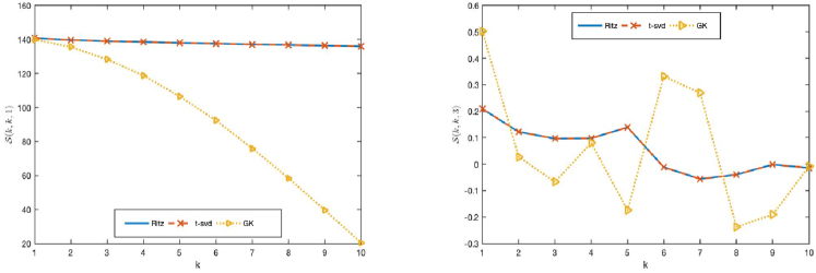
Refer to caption
Figure 2: The left-hand side pane shows the values of the first frontal slices (frames) of the first 101010 singular tubes computed by t-SVD, Ritz augmentation, and the partial Lanczos bidiagonalization (GK) method for a synthetic data of size 1000×1000×51000100051000\times 1000\times 5 with m=20𝑚20m=20. The right-hand side pane displays the third frontal slices of these tubes, i.e., 𝒮(k,k,i)𝒮𝑘𝑘𝑖\mathscr{S}(k,k,i) for k=1,2,,10𝑘1210k=1,2,\ldots,10 and i=1,3𝑖13i=1,3.
Refer to caption
Figure 3: Evolution of the remainder term for a third-order tensor of size 1000×1000×31000100031000\times 1000\times 3 when computing the first three singular triplets by Algorithm 6 with Ritz augmentation.

5.1.2 Smallest singular values

This subsection illustrates the performance of Algorithm 6 with Ritz augmentation (referred to as Ritz) and with harmonic Ritz augmentation (referred to as Harm) for computing the smallest singular triplets of synthetic third-order tensors of different sizes. Table 3 displays the error in the fourth smallest singular tubes computed by Ritz augmentation and harmonic Ritz augmentation for m=20𝑚20m=20, and compares with results determined by the t-SVD method. In Table 4 we show the number of iterations and the required CPU time (in seconds) for these methods when m=20𝑚20m=20.

i Method 100×100×31001003100\times 100\times 3 100×100×51001005100\times 100\times 5 500×500×35005003500\times 500\times 3 500×500×55005005500\times 500\times 5
n3𝑛3n-3 Ritz 3.82e-11 5.22e-12 1.34e-10 2.50e-10
Harm 1.03e-13 4.64e-13 4.66e-13 1.07e-13
n2𝑛2n-2 Ritz 1.99e-14 4.34e-13 1.20e-14 1.68e-11
Harm 4.94e-15 3.10e-13 2.46e-14 3.77e-14
n1𝑛1n-1 Ritz 8.36e-14 4.56e-14 1.77e-14 6.86e-12
Harm 1.64e-15 6.05e-15 2.88e-14 1.39e-13
n𝑛n Ritz 1.38e-15 7.71e-16 6.49e-15 2.00e-12
Harm 8.59e-16 7.90e-16 3.01e-15 1.41e-14
Table 3: The Frobenius norm 𝒮(i,i,:)𝚺(i,i,:)Fsubscriptnorm𝒮𝑖𝑖:𝚺𝑖𝑖:𝐹\left\|\mathscr{S}(i,i,:)-\bm{\Sigma}(i,i,:)\right\|_{F}, where 𝒮(i,i,:)𝒮𝑖𝑖:\mathscr{S}(i,i,:) denotes the singular tubes determined by Ritz augmentation or harmonic Ritz augmentation for m=20𝑚20m=20, and 𝚺(i,i,:)𝚺𝑖𝑖:\bm{\Sigma}(i,i,:) are tubes computed by the t-SVD method for the four smallest tubes, i.e., for i=n3,n2,n1,n𝑖𝑛3𝑛2𝑛1𝑛i=n-3,n-2,n-1,n.
Method 100×100×31001003100\times 100\times 3 500×500×35005003500\times 500\times 3 100×100×51001005100\times 100\times 5 500×500×55005005500\times 500\times 5
CPU time iter CPU time iter CPU time iter CPU time iter
Ritz 0.99 31 231.81 615 1.11 30 425.83 831
Harm 0.85 29 227.49 606 1.03 30 355.35 723
Table 4: CPU time in seconds, and number of iterations required by Algorithm 6 with Ritz augmentation and harmonic Ritz augmentation for m=20𝑚20m=20 to compute the four smallest singular triplets of synthetic third-order tensors of different sizes.

Tables 3 and 4 show that harmonic Ritz augmentation gives higher accuracy than Ritz augmentation when computing the smallest singular triplets. Figures 4 and 5 depict the Frobenius norm of the remainder term mmH𝒰isubscript𝑚superscriptsubscript𝑚𝐻subscript𝒰𝑖\vec{\mathscr{R}}_{m}\star\vec{\mathscr{E}}_{m}^{H}\star\vec{\mathscr{U}}_{i} for each iteration with Algorithm 6 with Ritz augmentation and harmonic Ritz augmentation when approximating the last two singular triplets for m=20𝑚20m=20.

Refer to caption
Figure 4: The Frobenius norm of mmH𝒰isubscript𝑚superscriptsubscript𝑚𝐻subscript𝒰𝑖\vec{\mathscr{R}}_{m}\star\vec{\mathscr{E}}_{m}^{H}\star\vec{\mathscr{U}}_{i} obtained by Algorithm 6 with Ritz augmentation when approximating the two smallest singular triplets of a synthetic tensor of size 500×500×55005005500\times 500\times 5 with m=20𝑚20m=20 at each iteration for i=499,500𝑖499500i=499,500.
Refer to caption
Figure 5: The Frobenius norm of mmH𝒰isubscript𝑚superscriptsubscript𝑚𝐻subscript𝒰𝑖\vec{\mathscr{R}}_{m}\star\vec{\mathscr{E}}_{m}^{H}\star\vec{\mathscr{U}}_{i} obtained by harmonic Ritz augmentation when approximating the last two singular triplets of a synthetic tensor data of size 500×500×55005005500\times 500\times 5 with m=20𝑚20m=20, at each iteration for i=499,500𝑖499500i=499,500.

Figures 4 and 5 show the error mmH𝒰iFsubscriptnormsubscript𝑚superscriptsubscript𝑚𝐻subscript𝒰𝑖𝐹\|\vec{\mathscr{R}}_{m}\star\vec{\mathscr{E}}_{m}^{H}\star\vec{\mathscr{U}}_{i}\|_{F} associated with Ritz augmentation in Algorithm 6 to converge in a smoother way than the corresponding error for harmonic Ritz augmentation. Both errors converge to zero as the number of iterations increases.

5.2 Application to data compression

Figure 6 displays examples of image compression using two color images: “house” of size 256×256×32562563256\times 256\times 3 and “Hawaii” of size 1200×1200×31200120031200\times 1200\times 3. For each image, we compute the k𝑘kth largest singular triplets using Ritz augmentation in Algorithm 6, which will be referred to as “Ritz,” for different numbers k𝑘k of desired singular triplets. Figure 7 displays the relative error of the compressed images for k=5,10,15,25𝑘5101525k=5,10,15,25, by using Ritz augmentation (Ritz) and the t-SVD method. This error is measured by

𝒜k𝒜F𝒜F,subscriptnormsubscript𝒜𝑘𝒜𝐹subscriptnorm𝒜𝐹\dfrac{\left\|\mathscr{A}_{k}-\mathscr{A}\right\|_{F}}{\left\|\mathscr{A}\right\|_{F}}, (44)

where 𝒜𝒜\mathscr{A} denotes the tensor that represents the original image and 𝒜k=i=1k𝒰i𝒔i𝒱Hsubscript𝒜𝑘superscriptsubscript𝑖1𝑘subscript𝒰𝑖subscript𝒔𝑖superscript𝒱𝐻\mathscr{A}_{k}=\sum_{i=1}^{k}\vec{\mathscr{U}}_{i}\star\bm{s}_{i}\star\vec{\mathscr{V}}^{H}.

Refer to caption
Figure 6: Examples of image compression applied to the “house” and “Hawaii” images for k=5,10,15,25𝑘5101525k=5,10,15,25 slices using Algorithm 6 with Ritz augmentation.
Refer to caption
Figure 7: Relative compression error (44) for the images “house” and “Hawaii” obtained with Algorithm 6 with Ritz augmentation (Ritz) and the t-SVD method.

Figure 7 shows the relative errors obtained with Algorithm 6 with Ritz augmentation and the t-SVD are almost the same. This means that the approximate singular tubes and the right and left singular lateral slices determined by Algorithm 6 with Ritz augmentation are very accurate.

5.3 Facial recognition

We illustrate the application of Algorithm 7 to facial recognition using color images that are represented by third-order tensors. The images in our test are from the Georgia Tech database GTDB__\_crop [26], which contains 750750750 images of 505050 persons, with each person represented by 151515 images that show various facial expressions and facial orientation, and different illumination conditions. Figure 8 shows an example of images of one person in the data set.
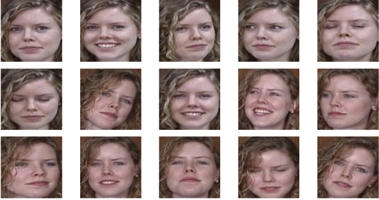
Refer to caption
Figure 8: An example of a person with different facial expressions and orientations.

Each image in the data set is of size 100×100×31001003100\times 100\times 3 pixels, and we use 333 randomly chosen images of each person as test images. The remaining 600600600 images form our training set and define the tensor 𝒳10000×600×3𝒳superscript100006003\mathscr{X}\in\mathbb{R}^{10000\times 600\times 3}. We applied Algorithm 7 and compared the results with those obtained by the t-SVD and also with results obtained by the‘ Golub-Kahan (GK) algorithm using the t-product. The performance of these methods is measured by the identification rate given by

Identification rate=number of correctly matched imagesnumber of test images×100(%).\text{Identification rate}=\dfrac{\text{number of correctly matched images}}{\text{number of test images}}\times 100(\%). (45)

Figures 9 and 10 show results obtained for k=1𝑘1k=1 and k=5𝑘5k=5 for two different persons. The mean image is defined as in Algorithm 7.

Refer to caption
Figure 9: A test for k=1𝑘1k=1.
Refer to caption
Figure 10: A test for k=5𝑘5k=5.
Refer to caption
Figure 11: Identification rates for different truncation indices k𝑘k by Ritz augmentation, t-SVD and Golub-kahan methods.

Figures 9 and 10 show that Algorithm 7 performs well for some values of the truncation index k𝑘k. In Figure 11, we plotted the identification rate (45) obtained with Algorithm 7 (Ritz augmentation), GK for m=k𝑚𝑘m=k, and with the exact t-SVD method for the 150150150 test images.

k 222 333 444
Method Ritz t-SVD Ritz t-SVD Ritz t-SVD
CPU time (s) 10.60 52.82 13.11 63.63 13.88 64.77
Table 5: CPU time (in seconds) for Algorithm 7 (Ritz) and for the t-SVD method for m=10𝑚10m=10 and different values of the truncation index k𝑘k.

Table 5 reports CPU times for Algorithm 7 for m=10𝑚10m=10 (Ritz) and for the t-SVD method for different values of the truncation index k𝑘k. The results show Algorithm 7 to be very effective both in terms of accuracy and CPU time compared to the t-SVD and the classical Golub-Kahan methods.

6 Conclusion and extensions

This paper presents two new methods for approximating the largest or smallest singular triplets of large third-order tensors using the t-product. We use restarted Lanczos bidiagonalization for third-order tensors to develop the Ritz augmentation method to determine the largest or smallest singular triplets. Moreover, we propose the harmonic Ritz augmentation method to compute the smallest singular triplets. These methods are applied to data compression and face recognition.

References

  • [1] T. Arnold, M. Kane, B. W. Lewis, A Computational Approach to Statistical Learning, CRC Press, Boca Raton, 2018.
  • [2] M. N. Asif, I. S. Bajwa, S. I. Hyder, M. Naweed, Feature based image classification by using principal component analysis, ICGST International Journal on Graphics, Vision and Image Processing. 9, 22–17 (2009).
  • [3] H. Avron, L. Horesh, M. E. Kilmer, E. Newman, Tensor-tensor algebra for optimal representation and compression of multiway data, Proceedings of the National Academy of Sciences, 188, 28 (2021)
  • [4] J. Baglama, V. Perovic, J. Picucci, Hybrid iterative refined restarted Lanczos bidiagonalization method, Numerical Algorithms, in press (2022).
  • [5] J. Baglama, L. Reichel, Augmented implicitly restarted Lanczos bidiagonalization methods, SIAM Journal on Scientific Computing, 27, 19–42 (2005).
  • [6] J. Baglama, L. Reichel, B. W. Lewis, irbla: Fast truncated singular value decomposition and principal component analysis, https://cran.r-project.org/web/packages/irlba/index.html.
  • [7] J. Baglama, L. Reichel, D. Richmond, An Augmented LSQR Method, Numerical Algorithms, 64, 263–293 (2013).
  • [8] J. Baglama, D. Richmond, Implicitly restarting the LSQR algorithm, Electronic Transactions on Numerical Analysis, 42, 85–105 (2014).
  • [9] F. P. A. Beik, M. Najafi-Kalyani, L. Reichel, Iterative Tikhonov regularization of tensor equations based on the Arnoldi process and some of its generalizations, Applied Numerical. Mathematics, 151, 425–447 (2020).
  • [10] A. H. Bentbib, A. EL Hachimi, K. Jbilou, A. Ratnani, A tensor regularized nuclear norm method for image and video completion, Journal of Optimization Theory and Applications, 192, 401–425 (2022).
  • [11] Å. Björck, A bidiagonalization algorithm for solving large and sparse ill-posed systems of linear equations, BIT Numerical Mathematics, 18, 659–670 (1988).
  • [12] D. Calvetti, L. Reichel, Tikhonov regularization of large linear problems, BIT Numerical Mathematics, 43, 263–283 (2003).
  • [13] Y. Chen, J. Feng, H. Lin, W. Liu, C. Lu, S. Yan, Tensor robust principal component analysis with a new tensor nuclear norm, IEEE Transactions on Pattern Analysis and Machine Intelligence, 42, 925–938 (2019).
  • [14] G. Golub, W. Kahan, Calculating the singular values and pseudo-inverse of a matrix, Journal of the Society for Industrial and Applied Mathematics, Series B: Numerical Analysis, 2, 205–224 (1965).
  • [15] M. El Guide, A. El Ichi, K. Jbilou and R. Sadaka, On tensor GMRES and Golub-Kahan methods via the T-product for color image processing, The Electronic Journal of Linear Algebra 37, 524–543 (2021).
  • [16] A. El Ichi, K. Jbilou, R. Sadaka, On tensor tubal-Krylov subspace methods, Linear and Multilinear Algebra, Linear and Multilinear Algebra, 37, 524–543 (2021).
  • [17] M. Hached, K. Jbilou, C. Koukouvinos, M. Mitrouli, A multidimensional principal component analysis via the C-product Golub-Kahan-SVD for classification and face recognition, Mathematics, 9, 1249 (2021).
  • [18] N. Hao, M. E. Kilmer, K. Braman, R. C. Hoover, Facial recognition using tensor-tensor decompositions, SIAM Journal on Imaging Sciences, 6, 437–463 (2013).
  • [19] M. E. Hochstenbach, A Jacobi-Davidson type SVD method, SIAM Journal on Scientific Computing, 23, 606–628 (2001).
  • [20] Z. Jia, D. Niu, A refined harmonic Lanczos bidiagonalization method and an implicitly restarted algorithm for computing the smallest singular triplets of large matrices, SIAM Journal on Scientific Computing, 32, 714–744 (2010).
  • [21] E. Kernfeld, M. Kilmer, S. Aeron, Tensor-tensor products with invertible linear transforms, Linear Algebra and Its Applications, 485, 545–570 (2015).
  • [22] M. E. Kilmer, K. Braman, N. Hao, R. C. Hoover, Third-order tensors as operators on matrices: A theoretical and computational framework with applications in imaging, SIAM Journal on Matrix Analysis and Applications, 34, 148–172 (2013).
  • [23] M. Kilmer, C. D. Martin, Factorization strategies for third-order tensors, Linear Algebra and Its Applications, 435, 641–658, (2011).
  • [24] E. Kokiopoulou, C. Bekas, E. Gallopoulos, Computing smallest singular triplets with implicitly restarted Lanczos bidiagonalization, Applied Numerical Mathematics, 49, 39–61 (2004).
  • [25] T. Kolda, B. W. Bader, Tensor decompositions and applications, SIAM Review, 51, 455–500 (2009).
  • [26] A.V. Nefian, Georgia Tech Face Database, Available online: http://www.anefian.com/research/face_reco.htm.
  • [27] C. C. Paige, B. N. Parlett, H. A. Van der Vorst, Approximate solutions and eigenvalue bounds from Krylov subspaces, Numerical Linear Algebra with Applications, 2, 115–133 (1995).
  • [28] C. C. Paige, M. A. Saunders, LSQR: An algorithm for sparse linear equations and sparse least squares, Transactions on Mathematical Software, 8, 43–71 (1982).
  • [29] P. K. Pandey, Y. Singh, S. Tripathi, Image processing using principle component analysis, International Journal of Computer Applications, 15, 37–40 (2011).
  • [30] L. Reichel, U. O. Ugwu, Tensor Krylov subspace methods with an invertible linear transform product applied to image processing, Applied Numerical Mathematics, 166, 186–207 (2021).
  • [31] L. Reichel and U. O. Ugwu, Tensor Arnoldi-Tikhonov and GMRES-type methods for ill-posed problems with a t-product structure, Journal of Scientific Computing, 90, Art. 59 (2022).
  • [32] L. Reichel, U. O. Ugwu, The tensor Golub-Kahan-Tikhonov method applied to the solution of ill-posed problems with a t-product structure, Numerical Linear Algebra with Applications, 29, e2412 (2022).
  • [33] H. Rojo, O. Rojo, Some results on symmetric circulant matrices and on symmetric centrosymmetric matrices, Linear Algebra and Its Applications, 391, 211-233 (2004).
  • [34] H. D. Simon, H. Zha, Low-rank matrix approximation using the Lanczos bidiagonalization process with applications, SIAM Journal on Scientific Computing, 21, 2257–2274 (2000).
  • [35] D. C. Sorensen, Implicit application of polynomial filters in a k𝑘k-step Arnoldi method, SIAM Journal on Matrix Analysis and Applications, 13, 357–385 (1992).
  • [36] A. Stathopoulos, Y. Saad, Restarting techniques for the (Jacobi-) Davidson symmetric eigenvalue methods, Electronic Transactions on Numerical Analysis, 7, 163–181 (1998).