Towards Long-Term Time-Series Forecasting: Feature, Pattern, and Distribution

Abstract

Long-term time-series forecasting (LTTF) has become a pressing demand in many applications, such as wind power supply planning. Transformer models have been adopted to deliver high prediction capacity because of the high computational self-attention mechanism. Though one could lower the complexity of Transformers by inducing the sparsity in point-wise self-attentions for LTTF, the limited information utilization prohibits the model from exploring the complex dependencies comprehensively. To this end, we propose an efficient Transformer-based model, named Conformer, which differentiates itself from existing methods for LTTF in three aspects: (i) an encoder-decoder architecture incorporating a linear complexity without sacrificing information utilization is proposed on top of sliding-window attention and Stationary and Instant Recurrent Network (SIRN); (ii) a module derived from the normalizing flow is devised to further improve the information utilization by inferring the outputs with the latent variables in SIRN directly; (iii) the inter-series correlation and temporal dynamics in time-series data are modeled explicitly to fuel the downstream self-attention mechanism. Extensive experiments on seven real-world datasets demonstrate that Conformer outperforms the state-of-the-art methods on LTTF and generates reliable prediction results with uncertainty quantification.

I Introduction

Time-series data evolve over time, which can result in perplexing time evolution patterns over the short- and long-term. The time evolution nature of time-series data is of great interest to many downstream tasks including time-series classification, outlier detection, and time-series forecasting. Among these tasks, time-series forecasting (TF) has attracted many researchers and practitioners in a wide range of application domains, such as transportation and urban planning [1], energy and smart grid management [2], as well as weather [3] and disease propagation analysis [4].

In many real-world application scenarios, given a substantial amount of time-series data recorded, there is a necessity to make a decision in advance, such that, with long-term prediction, the benefits can be maximized while the potential risks can be avoided. Therefore, in this work, we study the problem of forecasting time series that looks far into the future, namely long-term time-series forecasting (LTTF).

While tons of TF methods [5, 6, 7, 8] have been proposed with statistical learners, the use of domain knowledge however seems indispensable to model the temporal dependencies for TF but also limits the potential in applications. Recently, deep models [9, 10, 11, 12, 13] have been proposed for TF, which can be categorized into two types: the RNN-based and the Transformer-based models. RNN-based methods capture and utilize long- and short-term temporal dependencies to make the prediction, but fail to deliver good performance in long-term time-series forecasting tasks. Transformer-based models have achieved promising performance in extracting temporal patterns for LTTF because of the usage of self-attention mechanisms. However, such “full” attention mechanisms bring quadratic computation complexity for TF tasks, which thus becomes the main bottleneck for Transformer-based models to solve the long-term time-series forecasting task.

Several works have been devoted to improving the computation efficiency of self-attention mechanisms and lowering the complexity of handling a length-$L$ sequence to ($\mathcal{O}(L\log{L})$ or $\mathcal{O}(L\sqrt{L})$), such as Logtrans [14], Reformer [12], Informer [15] and Autoformer [13]. In the NLP field, some pioneering works have been proposed to reduce the complexity of self-attention to linear ($\mathcal{O}(L)$), including Longformer [16] and BigBird [17]. However, these deep models with a linear complexity might limit the information utilization and strain the performance of LTTF. Lowering the computational complexity to $\mathcal{O}(L)$ without sacrificing information utilization is a big challenge for LTTF.

In addition to the complexity, as the input length climbs up, the intricate time-series could exhibit obscure and confusing temporal patterns, which may lead to unstable prediction for self-attention-based models. Moreover, multivariate long-term time-series often embody multiple temporal patterns at different temporal resolutions, e.g., seconds, minutes, hours, or days. On the other hand, the intricate and prevailing multi-dimensional characteristics of the time-series data exhibit multi-faceted complex correlations among different series. Therefore, how to make the prediction for LTTF more stable and disaggregate multiscale dynamics and multivariate dependencies in time-series data are two more challenges.

To this end, our work devotes to the above three challenges and proposes a novel model based on Transformer for LTTF, namely Conformer. In particular, Conformer first explicitly explores the inter-series correlations and temporal dependencies with Fast Fourier Transform (FFT) plus multiscale dynamics extraction. Then, to address the LTTF problem in a sequence-to-sequence manner with linear computational complexity, an encoder-decoder architecture is employed on top of the sliding-window self-attention mechanism and the proposed stationary and instant recurrent network (namely, SIRN). More specifically, the sliding-window attention allows each point to attend to its local neighbors for reference, such that the self-attention dedicated to a length-$L$ time-series requires the $\mathcal{O}(L)$ complexity. Besides, to explore global signals in time-series data without violating the linear complexity, we renovate the cycle structure of the recurrent neural network (RNN) and distill stationary and instant patterns in long-term time-series with the series decomposition model in a recurrent way.

Moreover, to relieve the fluctuation effect caused by the aleatoric uncertainty [18] of time series data and improve the prediction reliability for LTTF, we further put efforts to model the underlying distribution of time-series data. To be specific, we devise a normalizing flow block to absorb latent states yielded in the SIRN model and generate the distribution of future series directly. More specifically, we leverage the outcome latent state of the encoder, as well as the latent state of the decoder, as input to initiate the normalizing flow. Afterward, the latent state of the decoder can be cascaded to infer the distribution of the target series. Along this line, the information utilization for LTTF can be further enhanced and the time-series forecasting can be implemented in a generative fashion, which is more noise-resistant.

Extensive experiments on seven real-world datasets validate that Conformer outperforms the state-of-the-art (SOTA) baselines with satisfactory margins. To sum up, our contributions can be highlighted as follows:

1. We reduce the complexity of self-attention to $\mathcal{O}(L)$ without sacrificing prediction capacity with the help of windowed attention and the renovated recurrent network.

2. We design a normalizing flow block to infer target series from hidden states directly, which can further improve the prediction and equip the output with uncertainty awareness.

3. Extensive experiments on five benchmark datasets and two collected datasets validate the superior long-term time-series forecasting performance of Conformer.

Figure 1: The framework overview of Conformer. In particular, the encoder extracts local patterns with sliding-window multi-head attention (MHA) and explores long-term trends and instant patterns with the proposed SIRN module. The decoder then receives long sequence inputs with the target elements being padded into zeros, measures the weighted composition of multi-faceted temporal patterns, and generates the prediction for target elements. At last, the normalizing flow block absorbs latent states yielded in the encoder-decoder architecture and predicts target elements with a chain of invertible transformations directly.

II Related Work

II-A Methods for Time-Series Forecasting

Many statistical methods have achieved big success in time-series forecasting (TF). For instance, ARIMA [5] is flexible to subsume multiple types of time-series but the limited scalability strains its further applications. Vector Autoregression (VAR) [6, 7] makes significant progress in multivariate TF by discovering dependencies between high-dimensional variables. Besides, there exist other traditional methods for the TF problem, such as SVR [8], SVM [19], etc., which also play important roles in different fields.

Another line of studies focuses on deep learning methods for TF, including RNN- and CNN-based models. For example, LSTM [20] and GRU [21] show their strengths in extracting the long- and short-term dependencies, LSTNet [1] combines the CNN and RNN to capture temporal dependencies in the time-series data, DeepAR [9] utilizes the autoregressive model, as well as the RNN, to model the distribution of future time-series. There are also some works focusing on CNN models [22, 23, 24, 25], which can capture inner patterns of the time-series data through convolution.

The Transformer [26] has shown its great superiority in NLP problems because of its effective self-attention mechanism, and it has been extended to many different fields successfully. There are many attempts to apply the Transformer to TF tasks, and the main idea lies in aiming to break the bottleneck of efficiency by focusing on the sparsity of the self-attention mechanism. The LogSparse Transformer [14] allows each point to attend to itself and its previous points with exponential step size, Reformer [12] explores the hashing self-attention, Informer [15] utilizes probability estimation to reduce the time and memory complexities, Autoformer [13] studies the auto-correlation mechanism in place of self-attention. All the above models reduce the complexity of self-attention to $\mathcal{O}(L\log L)$. The Sparse Transformer [27] reduces the complexity to $\mathcal{O}(L\sqrt{L})$ with attention matrix factorization. The very recent Longformer [16] and BigBird [17] adopt a number of attention patterns and can further reduce the complexity to $\mathcal{O}(L)$. However, the above reduction of complexity is often at the expense of sacrificing information utilization and the self-attention mechanism might not be reliable when temporal patterns are intricate in the LTTF task.

II-B Generative Models

There are works attempting to learn the distribution of future time-series data. Gaussian mixture model (GMM) [28] can learn the complex probability distribution with the EM algorithm, but it fails to suit dynamic scenarios. Wu et al. [29] proposed a generative model for TF by using the dynamic Gaussian mixture. [30] devises an end-to-end model to make coherent and probabilistic forecasts by generating the distribution of parameters. In addition, the authors of [31] proposed an autoregressive model to learn the distribution of the data and make the probabilistic prediction.

The variational inference was proposed for generative modeling and introduced latent variables to explain the observed data [32], which provides more flexibility in the inference. Both GAN [33] and VAE [34] show their impressive performances in distribution inference, but the cumbersome training process plus the limited generalization to new data hinder them for wider applications. Normalizing Flows (NFs) are a family of generative models, an NF is the transformation of a simple distribution that results in a more complex distribution. NF models have been applied in many fields successfully to learn intractable distribution, including image generation, noise modeling, video generation, audio generation, etc. Conformer employs the NF as an inner block for LTTF to absorb latent states in the encoder-decoder architecture, which differentiates itself from prior works.

III Problem Statement

We introduce the problem definition in this section. Given a length-$L$ time-series $\mathcal{X}=\{\mathbf{x}_{1},\mathbf{x}_{2},\cdots\,\mathbf{x}_{L}|\,\mathbf{x}_{i}\in\mathbb{R}^{d_{x}}\}$ where $\mathbf{x}_{i}$ is not limited to the univariate case (i.e., $d_{x}\geq 1$), the time series forecasting problem takes a length-$L_{x}$ time-series $\mathbf{X}=\{\mathbf{x}_{m+1},\cdots,\mathbf{x}_{m+{L_{x}}}\}$ as input to predict the future length-$L_{y}$ time series $\mathbf{Y}=\{\mathbf{x}_{n+1},\cdots,\mathbf{x}_{n+{L_{y}}}\}$ ($n=m+{L_{x}}$ and $m=1,\cdots,L-L_{y}$). For the sake of clarity, we denote $\mathbf{Y}=\{\mathbf{y}_{n+1},\cdots,\mathbf{y}_{n+{L_{y}}}\,|\,\mathbf{y}_{j}\in\mathcal{X}\}$. Long-term time-series forecasting is to predict the future time-series with larger $L_{y}$.

IV Methodology

The framework overview of Conformer is shown in Fig. 1. Conformer mainly consists of three parts: the input representation block, encoder-decoder architecture, and normalizing flow block. First, the input representation block preprocesses and embeds the input time series accordingly. Then, the encoder-decoder architecture explores the local temporal patterns with windowed attention from time-series representations and examines long-term intricate dynamics from both stationary and instant perspectives with the help of recurrent network and time-series decomposition. Moreover, to improve information utilization, the normalizing flow block leverages latent states in the recurrent network and generates target series from the latent states directly. The technical details of these three components will be introduced in the following subsections.

IV-A Input Representation

The time series data exhibits intricate patterns since multi-faceted underlying signals are often complex and varying. Given a length-$L$ time series $\mathcal{X}$, $\mathcal{X}=\{\mathbf{x}_{1},\mathbf{x}_{2},\cdots,\mathbf{x}_{L}|\mathbf{x}_{i}\in\mathbb{R}^{d_{x}}\}$ ($d_{x}\geq 1$), we investigate the underlying multi-faceted relatedness in $\mathcal{X}$ from two perspectives, i.e., the “vertical” feature perspective, and the “horizontal” temporal perspective.

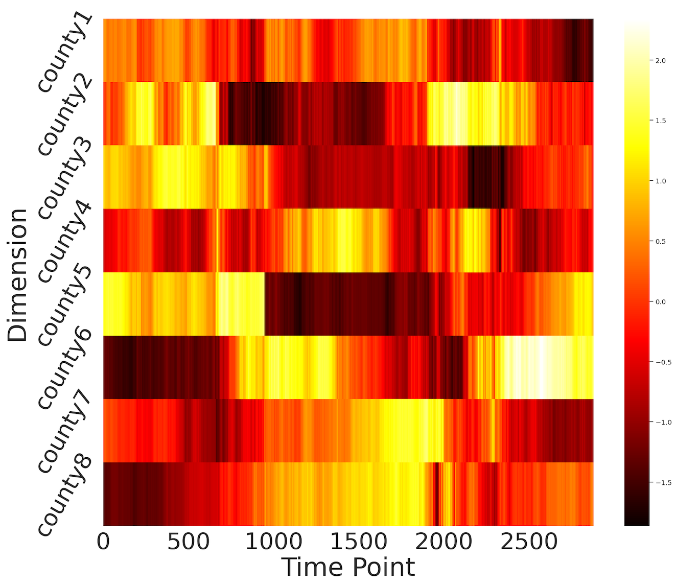
(a) Exchange rate.

(b) Wind power.

Figure 2: Different variables of time-series data evolve at varying rhythms and dynamics. The details of these datasets can be found in Section V-A1.

IV-A1 Multivariate Correlation

Complex relatedness among different variables in a multivariate time series hinders the effectiveness of distinguishing and harnessing important signals for future series prediction. On the one hand, the impacts of different variables on forecasting future series differ. For instance, the heatmaps in Fig. 2 illustrate rhythms of different variables in various time-series datasets, it is clear that different variables exhibit distinct relatedness to the target variable, which can also vary over time. On the other hand, the well-leveraged dependencies among variables can benefit time-series forecasting.

Fast Fourier Transform (FFT) [35] has been proven to be effective in discovering the correlations for time series data [36, 37, 38]. Inspired by this, we adopt FFT to represent implicit multivariate correlations of a length-$L$ time series by exploring the auto-correlation as follows:

$$\mathcal{MR}_{\mathcal{XX}}=f^{-1}(f(\mathcal{X})f^{\ast}(\mathcal{X}))\,,$$ (1)

where $f$ and $f^{-1}$ denote FFT and inverse FFT, respectively. The asterisk represents a conjugate operation. Besides, we employ Softmax to highlight informative variables accordingly:

$$\mathbf{W}^{\mathcal{R}}=\text{Softmax}(\mathcal{MR}_{\mathcal{XX}})\,.$$ (2)

IV-A2 Multiscale Dynamics

Temporal patterns are helpful in solving the long-term time-series forecasting problem [39]. We further examine the temporal patterns by means of multiscale representation. Specifically, a time series can present distinct temporal patterns at different temporal resolutions. In other words, more attention should be paid to informative dynamics extracted at certain temporal resolutions.

To implement the temporal pattern extraction at different scales, we first devise a temporal resolution set $S\subseteqq\{second,$ $minute,$ $hour,$ $day,$ $week,month,year\}$ for $\mathcal{X}$. Then the sampled time-series set ${\Gamma}^{S}=\{{\Gamma}^{S_{1}},\cdots,{\Gamma}^{S_{K}}\}$ is obtained, where $K$ denotes the number of temporal resolutions and ${\Gamma}^{S_{k}}$ is the sequence of sampled timestamps at corresponding temporal resolution $S_{k}$. Afterward, each series in ${\Gamma}^{S}$ is embedded into a latent space with $d\times L$ dimensionality, such that different series in ${\Gamma}^{S}$ are additive:

$$\tilde{{\Gamma}}^{S} =\mathcal{E}({\Gamma}^{S})=\{\mathcal{E}({\Gamma}^{S_{1}}),\cdots,\mathcal{E}({\Gamma}^{S_{K}})\}$$ (3)

$$=\{\tilde{{\Gamma}}^{S_{1}},\cdots,\tilde{{\Gamma}}^{S_{K}}\}\,,$$

where $\mathcal{E}$ denotes an embedding operation and $\tilde{{\Gamma}}^{S_{k}}\in\mathbb{R}^{d\times L}$ represents the embedded series at a certain temporal resolution $S_{k}$. Then the multiscale temporal patterns can be modeled as:

$$\bar{\Gamma}^{S} =\mathbf{W}^{S}\,\text{Concat}(\tilde{{\Gamma}}^{S})+(\mathbf{b}^{S})^{\prime}$$ (4)

$$=\sum_{k=1}^{K}\mathbf{W}_{k}^{S}\,(\tilde{\Gamma}^{S_{k}})^{\prime}+(\mathbf{b}^{S})^{\prime}\,,$$

where $\mathbf{W}^{S}\in\mathbb{R}^{L\times L\times K}$ and $\mathbf{b}^{S}\in\mathbb{R}^{d\times L}$ are trainable weights and bias, respectively. The prime symbol denotes the matrix transpose. Besides, $\mathbf{W}_{k}^{S}\in\mathbb{R}^{L\times L}$ denotes the $k$-th sliced matrix of $\mathbf{W}^{S}$.

IV-A3 Fusing Multivariate and Temporal Dependencies

Moreover, to make different variables in multivariate time series more distinguishable w.r.t. their importance for future series, we further apply the convolution to take temporal dependencies into account, which is defined as follows:

$$\mathcal{X}^{v}=\mathbf{W}^{v}\odot(\mathbf{W}^{\mathcal{R}}\,\mathcal{X}+\mathcal{X})+\mathbf{b}^{v}\,,$$ (5)

where $\odot$ denotes the convolution operation, and $\mathbb{W}^{v}\in\mathbb{R}^{d_{x}\times d}$ and $\mathbf{b}^{v}\in\mathbb{R}^{d\times L}$ denote weights and bias, respectively.

Finally, by combining the above multivariate correlations and multiscale dynamics with Eqs. 2 and 5, the outcome time-series representation can be obtained as follows:

$$\mathcal{X}^{in}=\mathcal{X}^{v}+\bar{\Gamma}^{S}\,.$$ (6)

IV-B Encoder-Decoder Architecture

Our proposed Conformer adopts the encoder-decoder architecture for long-term time-series forecasting.

IV-B1 Attention Mechanism

The standard attention mechanism [26] takes a three-tuple $(query,key,value)$ as input and employs the scaled dot product and Softmax to calculate the weights against the value as: $\text{Attn}(Q,K,V)=\text{Softmax}(\frac{QK^{T}}{\sqrt{d_{k}}})V$, where $Q\in\mathbb{R}^{L\times d_{k}}$, $K\in\mathbb{R}^{L\times d_{k}}$, and $V\in\mathbb{R}^{L\times d_{v}}$ represent query, key and value, respectively.

Moreover, the multi-head attention (MHA) [26] employs projections for the original query, key, and value $N$ times, and the $i$-th projected query, key, and value can be obtained by $Q_{i}=QW^{Q}_{i}$, $K_{i}=KW_{i}^{K}$, and $V_{i}=VW^{V}_{i}$, where $W_{i}^{Q}\in\mathbb{R}^{d_{k}\times d_{k}/N}$, $W_{i}^{K}\in\mathbb{R}^{d_{k}\times d_{K}/N}$, and $W_{i}^{V}\in\mathbb{R}^{d_{v}\times d_{v}/N}$. Afterward, the attention can be applied to these queries, keys, and values in parallel, and the outcome is further concatenated and projected as follows:

$$\text{ha}_{i}= \text{Attn}(Q_{i},K_{i},V_{i}),\quad i=1,2,\cdots,N$$ (7)

MHA $$(Q,K,V)=\text{Concat}(\text{ha}_{1},\text{ha}_{2},\cdots,\text{ha}_{N})W^{o}\,.$$

Sliding-Window Attention.  Duplicated messages exist across different heads in full self-attention [40]. A time series often shows a strong locality of reference, thus a great deal of information about a point can be derived from its neighbors. Hence, the full attention message might be too redundant for future series prediction. Given the importance of locality for TF, the sliding-window attention (with fixed window size $w$) allows each point attends to its $\frac{1}{2}w$ neighbors on each side. Thus, the time complexity of this pattern is $\mathcal{O}(w\times L)$, which scales linearly with input length. Therefore, we adopt this windowed attention to realize self-attention.

IV-B2 Stationary and Instant Recurrent Network

Although the windowed attention can reduce the complexity to $\mathcal{O}(L)$, the information utilization could be sacrificed for LTTF due to point-wise sparse connections. RNNs have achieved big successes in many sequential data applications [41, 42, 43, 44] attributed to their capabilities of capturing dynamics in sequences via cycles in the network of nodes. To enhance information utilization without increasing time and memory complexities, we, therefore, renovate the recurrent network accordingly. In particular, we not only distill the stationary (trend) and instant (seasonal) temporal patterns from input series but also integrate the distilled long-term patterns, as well as the aforementioned local temporal patterns, into the time-series representation. The architecture of the proposed Stationary and Instant Recurrent Network (SIRN) is demonstrated in Fig. 3(a).

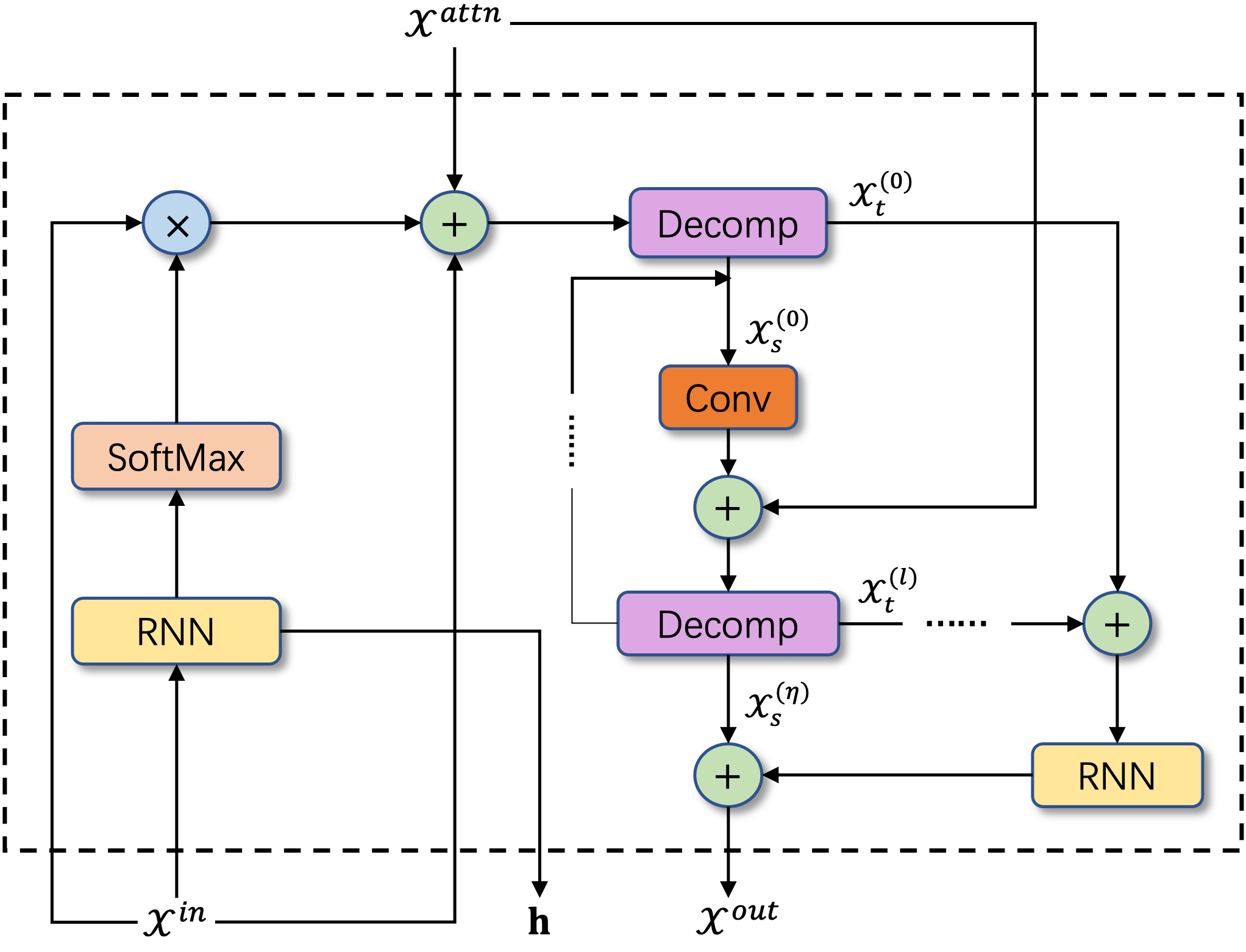
(a) Stationary and instant recurrent network (SIRN).

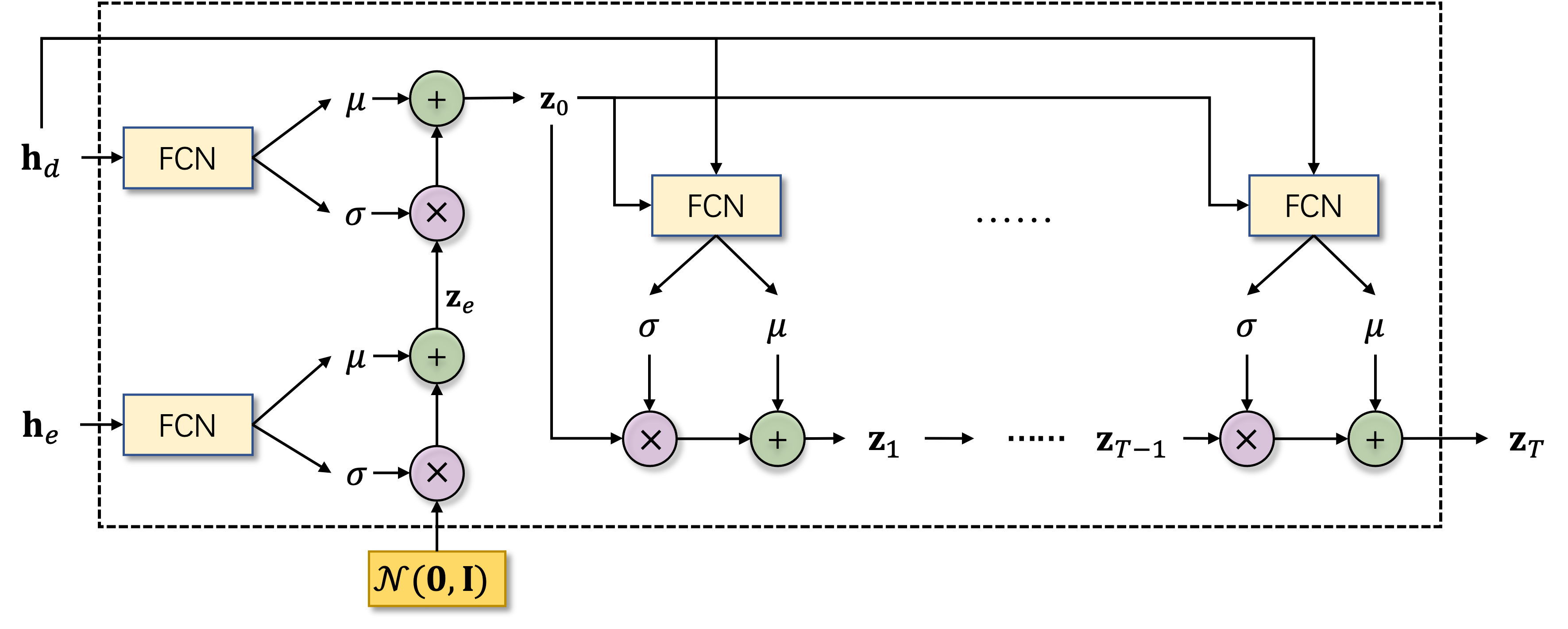
(b) Normalizing flow framework.

Figure 3: The architecture of SIRN and the normalizing flow framework. (a) The first RNN block embeds the global information of input time-series and the second RNN block represents the aggregated trend information extracted by the decomposition block. The decomposition procedure following the initial decomposition can be repeated multiple times. The latent state yielded by the first RNN will be utilized in the normalizing flow framework. (b) After initiating the flow of transformations with Eqs. 15 and 16, the latent state of decoder is adopted to generate the target variable.

Specifically, we feed the input representation to the first RNN block (followed by a Softmax) to initialize the global representation and add it to the local representation, as well as the original input representation, as follows:

$$\mathcal{X}^{in}= \text{SoftMax}(\text{RNN}(\mathcal{X}^{in}))\times\mathcal{X}^{in}$$ (8)

$$+\text{MHA}_{W}(\mathcal{X}^{in})+\mathcal{X}^{in}\,,$$

where $\text{MHA}_{W}(\cdot)$ denotes the sliding-window attention. Note that the RNN block (followed by Softmax) in the first term of Eq. 8 aims to capture the global temporal dependency, which can supplement the local dependency captured by the windowed attention.

Though intricate and diverse, the complex temporal patterns in different time-series data can be roughly divided into (coarse-grained) stationary trends and (fine-grained) instant patterns. Along this line, we employ the series decomposition introduced in [45, 13] to distill stationary and instant patterns by capturing trend and seasonal parts of the time-series data. Similar to [13], we adopt the moving average to capture long-term trends and the residual of the original series subtracting the moving average as seasonal patterns:

$$\mathcal{X}_{t}=\text{AvgPool}(\text{Padding}(\mathcal{X}^{in})),\quad\mathcal{X}_{s}=\mathcal{X}^{in}-\mathcal{X}_{t},$$ (9)

where $\mathcal{X}_{t},\mathcal{X}_{s}\in\mathbb{R}^{L\times d_{x}}$ denote the trend and seasonal parts of $\mathcal{X}^{in}$, respectively. Then, we use a convolution layer to embed the seasonal pattern. And, we feed the embedded representation, coupled with the local representation, to another decomposition block for distilling more seasonal patterns. This distillation process can be implemented in a recurrent way:

$$\mathcal{X}_{t}^{(l)},\mathcal{X}_{s}^{(l)} =\text{Decomp}(\text{Conv}(\mathcal{X}_{s}^{(l-1)})$$ (10)

$$+\text{MHA}_{W}(\mathcal{X}^{in})),\,\,l=1,\cdots,\eta\,,$$

where Decomp denotes Eq. 9, $\mathcal{X}_{s}^{(0)}=\mathcal{X}_{s}$ and $\mathcal{X}_{t}^{(0)}=\mathcal{X}_{t}$. On the other hand, the trend parts generated by different decompositions are merged and fed to the second RNN block. Finally, the distilled multi-faceted temporal dynamics are fused to generate the outcome representation:

$$\mathcal{X}^{out}=\mathbf{W}(\mathcal{X}_{s}^{(\eta)}+\text{RNN}(\sum_{l=0}^{\eta}\mathcal{X}_{t}^{(l)})).$$ (11)

IV-C Time Series Prediction with Normalizing Flow

The aforementioned SIRN framework adopts RNN to extract global signals. In addition, the hidden states yielded by RNN are beneficial for understanding the distribution of time-series data. Specifically, we design a normalizing-flow block to learn the distribution of hidden states to increase the reliability of prediction.

IV-C1 Background of Normalizing Flow

A time series $\mathcal{X}=\{\mathbf{x}_{1},$ $\cdots,$ $\mathbf{x}_{L}\}$ can be reconstructed by maximizing the marginal log-likelihood: $\log p(\mathcal{X})=\sum_{i=1}^{L}\log p(\mathbf{x}_{i})$. Due to the intractability of such log-likelihood, a parametric inference model over the latent variables $\mathbf{z}$, i.e., $q(\mathbf{z}|\mathbf{x})$, was introduced. Then, one can optimize the variational lower bound on the marginal log-likelihood of each observation $\mathbf{x}$ as follows:

$$\log p(\mathbf{x})\geqslant \mathbb{E}_{q(\mathbf{z}|\mathbf{x})}[\log p(\mathbf{x},\mathbf{z})-\log q(\mathbf{z},\mathbf{x})]$$ (12)

$$= \log p(\mathbf{x})-\mathcal{D}_{KL}(q(\mathbf{z}|\mathbf{x})\,||\,p(\mathbf{z}|\mathbf{x}))$$

$$= \mathcal{L}(\mathbf{x};\theta)\,,$$

where $\mathcal{D}_{KL}(\cdot)$ denotes the Kullback-Leibler divergence. When the dimensionality of $\mathbf{z}$ climbs up, the diagonal posterior distribution is often adopted, which is, however, not flexible enough to match the complex true posterior distributions [46]. To solve this, the Normalizing Flow [47] was proposed to build flexible posterior distributions.

Basically, one can start off with an initial random variable $\mathbf{z}_{0}$ (with a simple distribution, coupled with a known density function), and then apply a chain of invertible transformations $\text{f}_{t}$, such that the outcome $\mathbf{z}_{T}$ has a more flexible distribution:

$$\mathbf{z}_{0}\backsim q(\mathbf{z}_{0}|\mathbf{x}),\quad\mathbf{z}_{t}=\text{f}_{t}(\mathbf{z}_{t-1}),\quad t=1,\cdots,T\,.$$ (13)

Besides, as long as the Jacobian determinant $\det\left|\frac{d\mathbf{z}_{t}}{d\mathbf{z}_{t-1}}\right|$ is available, the transformation can take the following definition:

$$\text{f}_{t}(\mathbf{z}_{t-1})=\mathbf{z}_{t-1}+\mathbf{u}\,g(\mathbf{w}^{T}\mathbf{z}_{t-1}+{b})\,,$$ (14)

where $\mathbf{u}$, $\mathbf{w}$ and $b$ are parameters, and $g(\cdot)$ denotes a nonlinear function.

IV-C2 Normalizing Flow for LTTF

The proposed architecture of normalizing flow in Conformer is shown in Fig. 3(b).

Let $\mathbf{h}$ denote the hidden state yielded by the first RNN block in SIRN. Then, draw a random variable from a Gaussian distribution, i.e., $\bm{\epsilon}\backsim\mathcal{N}(\mathbf{0},\mathbf{I})$, and the distribution of the hidden state in the encoder can be obtained as:

$$\mathbf{z}_{e}=\text{FCN}_{\mu}^{(e)}(\mathbf{h}_{e})+\text{FCN}_{\sigma}^{(e)}(\mathbf{h}_{e})\cdot{\bm{\epsilon}}\,,$$ (15)

where $\text{FCN}_{\mu}^{(e)}$ and $\text{FCN}_{\sigma}^{(e)}$ are two fully connected networks, $\mathbf{h}_{e}$ denotes the hidden state in encoder. Afterward, we take the latent representation $\mathbf{z}_{e}$ and the decoder latent state $\mathbf{h}_{d}$ as input to initiate the normalizing flow:

$$\mathbf{z}_{0}=\text{FCN}_{\mu}^{(d)}(\mathbf{h}_{d})+\text{FCN}_{\sigma}^{(d)}(\mathbf{h}_{d})\cdot\mathbf{z}_{e}\,.$$ (16)

Now that the normalizing flow can be iterated as follows:

$$\mathbf{z}_{t}= \,\,\text{FCN}_{\mu}^{(t)}(\mathbf{h}_{d},\mathbf{z}_{t-1})$$ (17)

$$+ \,\,\text{FCN}_{\sigma}^{(t)}(\mathbf{h}_{d},\mathbf{z}_{t-1})\cdot\mathbf{z}_{t-1},\quad t=1,\cdots,T\,.$$

Here, we utilize the decoder latent state to cascade the message, such that the future series can be generated directly.

IV-D Loss Function

In order to coordinate with the other parts of Conformer, the commonly used log-likelihood is substituted for the MSE (mean squared error) loss function for learning the normalizing flow framework. In particular, the random variable sampled from the outcome distribution, i.e., $\mathbf{z}_{t}$, is deemed as the point estimation of the target series. Then, we adopt MSE loss functions on prediction w.r.t. the target series for both encoder-decoder architecture and normalizing flow framework. Finally, the loss function is defined as follows:

$$\mathcal{L}=\lambda\cdot\text{MSE}(\mathbf{Y}^{out},\mathbf{Y})+(1-\lambda)\cdot\text{MSE}(\mathbf{Z}^{out},\mathbf{Y})$$ (18)

where $\mathbf{Y}^{out}$ and $\mathbf{Z}^{out}$ denote the output of decoder and normalizing flow, respectively, and $\lambda$ is a trade-off hyperparameter balancing the relative contributions of encoder-decoder and normalizing flow.

V Experiments

V-A Experiment Settings

V-A1 Datasets

We conduct experiments on seven datasets including five benchmark datasets and two collected datasets. Table I describes some basic statistics of these datasets.

ECL was collected in 15-minute intervals from 2011 to 2014. We select the records from 2012 to 2014 since many zero values exist in 2011 [1]. The processed dataset contains the hourly electricity consumption of 321 clients. We use ’MT_321’ as the target, and the train/val/test is 12/2/2 months.

Weather was recorded in 10-minute intervals from 07/2020 to 07/2021. There exist 21 meteorological indicators, e.g., the amount of rain, humidity, etc. We choose temperature as the target, and the train/val/test is 10/1/1 months.

Exchange [1] records the daily exchange rates of eight countries from 1990 to 2016. We use the exchange rates of Singapore as the target, The train/val/test is 16/2/2 years.

ETT [15] records the electricity transformer temperature. Every data point consists of six power load features and the target value is “oil temperture”. This dataset is separated into {ETTh1, ETTh2} and {ETTm1, ETTm2} for 1-hour-level and 15-minute-level observations, respectively. We use ETTh1 and ETTm1 as our datasets. The train/val/test are 12/2/2 and 12/1/1 months for ETTh1 and ETTm1, respectively.

Wind (Wind Power) records the generated wind power of a wind farm in 15-minute intervals from 01/2020 to 07/2021. The train/val/test is 12/1/1 months.

AirDelay was collected from the “On-Time” database in the TranStas data library. We extracted the flights arrived at the airports in Texas and examined arrival delays in the first month of the year 2022, and the canceled flights were removed. Note that the time interval of this dataset is varying. This dataset was split into train/val/test as 7:1:2.

TABLE I: Statistical descriptions of the time-series datasets.

Datasets	# Dims.	Time Span	# Points	Target Variable	Interval
ECL	321	01/2012 - 12/2014	26304	MT_321	1 hour
Weather	21	01/2020 - 06/2021	36761	Temperature	10 mins
Exchange	8	01/1990 - 12/2016	7588	Country8	1 day
ETTh1	7	07/2016 - 07/2018	17420	OT	1 hour
ETTm1	7	07/2016 - 07/2018	69680	OT	15 mins
Wind	7	01/2020 - 05/2021	45550	Wind_Power	15 mins
AirDelay	6	01/01 - 01/31, 2022	54451	ArrDelay	–

V-A2 Baselines

We compare Conformer with 9 baselines, i.e., 5 Transformer methods (Autoformer, Informer, Reformer, Longformer, and LogTrans), 2 RNN methods (GRU and LSTNet), and 2 other deep methods (TS2Vec and N-Beats).

TABLE II: Comparisons of multivariate LTTF results (the best and 2nd best scores are boldfaced and underlined, resp.).

Model		Transformer-based										RNN-based				Others
		Conformer		Longformer [16]		Autoformer [13]		Informer [15]		Reformer [12]		LSTNet [1]		GRU [21]		N-beats[48]
Metric		MSE	MAE	MSE	MAE	MSE	MAE	MSE	MAE	MSE	MAE	MSE	MAE	MSE	MAE	MSE	MAE
ECL	96	0.2124	0.3193	0.3156	0.3939	0.2018	0.3100	0.5423	0.5568	0.9865	0.7795	1.1002	0.8066	0.7292	0.6274	1.3759	0.8753
	192	0.2378	0.3456	0.3371	0.4169	0.3579	0.4277	0.5304	0.5549	1.0119	0.7831	1.0965	0.8048	1.0093	0.7679	1.3228	0.8660
	384	0.2643	0.3620	0.3976	0.4183	0.4670	0.5019	0.6429	0.5921	1.0883	0.7867	1.1034	0.8057	1.0548	0.7898	1.3911	0.8709
	768	0.3396	0.4092	0.5651	0.5182	0.5525	0.5598	0.9534	0.7789	1.0624	0.7913	1.1132	0.8085	1.0651	0.7938	1.3645	0.8585
Weather	48	0.3216	0.3433	0.3475	0.3630	0.4552	0.4340	0.3929	0.3231	0.5099	0.4506	0.7852	0.6769	0.6569	0.5438	0.6171	0.5346
	192	0.4129	0.4170	0.4259	0.4235	0.4965	0.4711	0.4396	0.4332	0.6960	0.5852	0.7858	0.6770	0.7548	0.6025	0.6121	0.5402
	384	0.4997	0.4847	0.5518	0.5030	0.5832	0.5255	0.5848	0.5197	0.7525	0.6231	0.8063	0.6886	0.7679	0.6070	0.6032	0.5067
	768	0.6146	0.5603	0.6734	0.5769	0.6429	0.5682	0.7051	0.5881	0.7883	0.6529	0.8303	0.7003	0.7671	0.6100	0.5944	0.5143
Exchange	48	0.0764	0.2093	0.1736	0.3314	0.1431	0.2892	0.2310	0.3841	0.3653	0.4952	1.0319	0.8623	1.1399	0.9119	2.1053	1.0750
	96	0.1193	0.2607	0.3519	0.4829	0.2021	0.3586	0.3079	0.4488	0.9120	0.7731	1.0260	0.8648	1.3953	0.9837	1.8161	0.9896
	192	0.2900	0.4187	0.6145	0.6393	0.4249	0.5486	0.5902	0.6306	1.1195	0.8713	0.9954	0.8562	1.3754	0.9800	1.8113	0.9899
	384	0.4730	0.5369	0.8105	0.7513	1.2798	0.9983	0.8630	0.7953	1.2748	0.9435	0.9642	0.8457	1.3801	0.9858	2.4088	1.1708
ETTm1	96	0.6854	0.5901	1.0947	0.7079	0.8586	0.6591	1.0921	0.7023	1.6397	0.9771	1.6250	0.9045	1.7469	0.9714	1.2350	2.3957
	192	0.7856	0.6387	1.2555	0.7644	0.9406	0.6958	1.2657	0.7898	1.6499	0.9659	1.6012	0.9080	1.7223	0.9592	1.2253	2.3467
	384	0.9298	0.6988	1.2303	0.7786	1.1112	0.7593	1.3849	0.8459	1.6396	0.9783	1.5063	0.8916	1.5815	0.9124	1.2149	2.2922
	768	0.9835	0.7193	1.2247	0.7816	1.2974	0.7940	1.3537	0.8492	1.6121	0.9501	1.3637	0.8604	1.3437	0.8425	1.2420	2.3629
ETTh1	96	0.6978	0.5623	0.7276	0.5894	0.7515	0.5727	0.8901	0.6498	0.9794	0.6926	1.1763	0.7884	1.0490	0.7312	1.6426	0.9352
	192	0.8444	0.6249	0.9074	0.6566	0.9346	0.6375	1.0463	0.7082	1.0157	0.7156	1.1850	0.7870	1.0850	0.7469	1.7524	0.9709
	384	0.9708	0.6767	0.9804	0.6919	1.1832	0.7347	1.1237	0.7383	1.0673	0.7298	1.2493	0.8082	1.1081	0.7471	1.7703	0.9778
	768	1.0827	0.7275	1.0501	0.7083	1.2562	0.7676	1.1047	0.7292	1.1105	0.7447	1.5301	0.9207	1.1275	0.7524	1.7656	0.9822
Wind	48	0.9479	0.6539	0.9605	0.6767	1.3522	0.8099	1.0056	0.6552	1.1881	0.7949	1.3874	0.9246	1.1599	0.8022	1.5667	0.8727
	96	1.1725	0.7641	1.2467	0.7698	1.4859	0.8702	1.2371	0.7994	1.3283	0.8529	1.4489	0.9441	1.2797	0.8455	1.6842	0.9074
	192	1.3291	0.8464	1.4829	0.8487	1.6118	0.9172	1.5022	0.8489	1.4074	0.8980	1.4794	0.9508	1.3779	0.8866	1.6146	0.8839
	384	1.3644	0.8692	1.5479	0.8830	1.7363	0.9585	1.5002	0.8747	1.4541	0.9190	1.4966	0.9541	1.3818	0.8897	1.5746	0.8551
	768	1.3698	0.8905	1.4995	0.8954	1.6629	0.9426	1.5152	0.8956	1.5215	0.9540	1.4813	0.9471	1.4580	0.9253	1.6176	0.9009
AirDelay	96	0.7491	0.5702	0.7746	0.5984	0.7959	0.6041	0.7663	0.5904	0.7719	0.5961	0.7781	0.6058	0.7675	0.5859	0.7961	0.5940
	192	0.7523	0.5689	0.7770	0.5980	0.7865	0.5934	0.7659	0.5876	0.7724	0.5960	0.7782	0.6053	0.7705	0.5903	0.8041	0.5961
	384	0.7560	0.5718	0.7876	0.6051	0.7896	0.5889	0.7729	0.5841	0.7735	0.5963	0.7784	0.6049	0.7739	0.5968	0.8082	0.5988
	768	0.7614	0.5729	0.8081	0.6209	0.7952	0.5921	0.7868	0.6061	0.7749	0.5956	0.7797	0.6044	0.7750	0.5961	0.8099	0.5981

1. GRU [21]: GRU employs the gating mechanism such that each recurrent unit adaptively captures temporal signals in the series. In this work, we adopt a 2-layer GRU.

2. LSTNet [1]: LSTNet combines the convolution and recurrent networks to extract short-term dependencies among variables and long-term trends in the time series. Note that, to simplify the parameter tuning, the highway and skip connection mechanisms are omitted.

3. N-Beats [48]: N-Beats was proposed to address time-series forecasting via a deep model on top of the backward and forward residual links and a very deep stack of fully-connected layers. We implement N-Beats for multivariate LTTF with suggested settings.

4. Reformer [12]: Reformer uses locality-sensitive hashing (LSH) attention and reversible residual layers to reduce the computation complexity. We implement Reformer by setting the bucket_length and the number of rounds for LSH attention as 24 and 4, respectively.

5. Longformer [16]: Longformer combines the windowed attention with a task motivated global attention to scale up linearly as the sequence length grows.

6. LogTrans [14]: LogTrans breaks the memory bottleneck of Transformer for LTTF via producing queries and keys with the help of causal convolutional self-attention. The number of the LogTransformer blocks is set to 2 and the sub_len of the sparse-attention is set to 1.

7. Informer [15]: Informer proposes the ProbSparse slef-attention to reduce time and memory complexities, and handles the long-term sequence with self-attention distilling operation and generative style decoder.

8. Autoformer [13]: Autoformer renovates the series decomposition with the help of auto-correlation mechanism, and put the series decomposition as a basic inner block of the deep model.

9. TS2Vec [49]: TS2Vec is a universal framework for learning representations of time series. It performs contrastive learning in a hierarchical way over augmented context views, which leads to the robust contextual representation for each timestamp. We implement TS2Vec for univariate LTTF with the suggested settings.

All baselines employ the one-step prediction strategy. For the RNN-based methods, the number of hidden states is chosen from $\{16,24,32,64\}$. For the Transformer-based methods, the number of heads of the self-attention is 8 and the dimensionality is set as 512 for all attention mechanisms in the experiments. Moreover, the sampling factor of the self-attention is set to 1 for both Informer and Autoformer, other settings are the same as suggested by [13]. All Transformer-based baselines (except Autoformer) use the same embedding method applied to the Informer. As suggested by [13], we omit the position embedding and keep the value embedding and timestamp embedding for Autoformer.

V-A3 Implementation Details

Conformer includes a 2-layer encoder and a 1-layer decoder, as well as a 2-layer normalizing flow block. The window size of the sliding-window attention is 2, and $\lambda$ in Eq. 18 is set to $0.8$. We use an Adam optimizer, and the initial learning rate is $1\times 10^{-4}$. The batch-size is 32 and the training process employs early stopping within 10 epochs. In addition, we use MAE (mean absolute error) and MSE (mean squared error) as the evaluation metrics.

An input-$L_{x}$-predict-$L_{y}$ window is applied to roll the train, validation and test sets with stride one time step, respectively. This setting is adopted for all datasets. The input length $L_{x}$ is 96 and the predict length $L_{y}$ is chosen from {48, 96, 192, 384, 768} on all datasets. The averaged results in 5 runs are reported. All models are implemented in PyTorch and trained/tested on a Linux machine with one A100 40GB GPU.

All of the RNN blocks in Conformer are implemented with GRU. Under the multivariate LTTF setting, we adopt 1-layer GRU and 2-layer GRU for encoder and decoder, respectively. Under the univariate LTTF setting, both the encoder and decoder adopt 1-layer GRU.

TABLE III: Multivariate LTTF with time-determined lengths (boldface and underline for the best and 2nd best scores).

Model		Transformer-based										RNN-based				Others
		Conformer		Longformer [16]		Autoformer [13]		Informer [15]		Reformer [12]		LSTNet [1]		GRU [21]		N-beats[48]
Metric		MSE	MAE	MSE	MAE	MSE	MAE	MSE	MAE	MSE	MAE	MSE	MAE	MSE	MAE	MSE	MAE
ETTh1	1D	0.4158	0.4434	0.3924	0.4316	0.4248	0.4374	0.3985	0.4345	0.6987	0.5640	1.1549	0.7713	0.9265	0.6771	0.9027	1.5612
	1W	0.7326	0.5785	0.7583	0.5997	0.8682	0.6130	0.8585	0.6362	1.0286	0.7207	1.2254	0.8020	1.1184	0.7571	0.9388	1.6576
	2W	0.8661	0.6400	0.9328	0.6767	1.1191	0.7126	1.0686	0.7054	1.0796	0.7378	1.2231	0.7964	1.1095	0.7456	0.9533	1.6852
	1M	0.9845	0.6887	0.9205	0.6763	1.2151	0.7567	1.0292	0.6887	1.1092	0.7451	1.6012	0.9525	1.1341	0.7566	1.0084	1.8501
ETTm1	1D	0.6854	0.5901	1.0947	0.7079	0.8586	0.6591	1.0921	0.7023	1.6397	0.9771	1.6250	0.9045	1.7469	0.9714	1.2350	2.3957
	1W	0.9540	0.7009	1.2416	0.7912	1.2016	0.7660	1.4284	0.8551	1.4008	0.8697	1.3692	0.8576	1.3852	0.8551	1.2322	2.3267
	2W	1.0948	0.7583	1.2463	0.7871	1.5101	0.8469	1.2857	0.8177	1.2233	0.7952	1.2931	0.8326	1.2245	0.7945	1.2540	2.3790

TABLE IV: Comparisons of univariate LTTF results (the best and 2nd best scores are boldfaced and underlined, resp.).

Model		Transformer-based										RNN-based				Others
		Conformer		Autoformer [13]		Informer [15]		Reformer [12]		LogTrans [14]		LSTNet [1]		GRU [21]		TS2VEC[49]
Metric		MSE	MAE	MSE	MAE	MSE	MAE	MSE	MAE	MSE	MAE	MSE	MAE	MSE	MAE	MSE	MAE
ECL	96	0.3481	0.4587	0.4457	0.5295	0.3182	0.4425	0.7945	0.7286	0.6378	0.6859	0.9617	0.7872	0.8348	0.7358	1.1987	2.1247
	192	0.3565	0.4629	0.5327	0.5787	0.3906	0.4968	0.8575	0.7465	0.6373	0.6837	0.9929	0.7904	0.9379	0.7700	1.1557	2.0041
	384	0.3659	0.4656	0.6592	0.6506	0.4352	0.5260	0.9269	0.7666	0.6369	0.6807	1.0074	0.7928	0.9685	0.7784	1.1863	2.0864
	768	0.4283	0.4989	0.7821	0.7190	0.4987	0.5674	0.9521	0.7711	0.6468	0.6815	1.0429	0.8034	0.9917	0.7847	1.0891	1.7940
Weather	48	0.0846	0.2025	0.1719	0.3073	0.0914	0.2183	0.1809	0.3202	0.3231	0.4460	0.4818	0.5985	0.3660	0.4689	1.6989	3.8099
	192	0.1898	0.3114	0.2365	0.3562	0.2008	0.3330	0.3597	0.4651	0.3115	0.4270	0.4947	0.5994	0.4505	0.5232	1.6884	3.7227
	384	0.3006	0.4041	0.3249	0.4345	0.3095	0.4267	0.4386	0.5198	0.3500	0.4554	0.5218	0.6171	0.4869	0.5383	1.4820	3.1272
	768	0.4005	0.4811	0.4665	0.5314	0.5536	0.5891	0.4493	0.5240	0.4297	0.5065	0.5414	0.6302	0.5397	0.5508	1.7431	3.9300
Exchange	48	0.0676	0.2059	0.1446	0.2892	0.2308	0.3840	0.3655	0.4954	0.2768	0.4338	1.0319	0.8623	1.1399	0.9858	1.2644	2.2181
	96	0.1168	0.2693	0.1369	0.2935	0.1827	0.3408	1.5431	1.0742	0.1976	0.3432	1.7163	1.2134	2.2484	1.3663	1.2797	2.2738
	192	0.2107	0.3751	0.4256	0.5549	0.3889	0.5021	2.0076	1.2959	0.5285	0.6217	1.6056	1.1823	2.5891	1.5426	1.2846	2.3074
	384	0.4591	0.5770	1.2899	1.0128	1.1126	0.7888	2.2899	1.4411	0.5520	0.6415	1.5664	1.1789	2.5353	1.5355	1.2947	2.3176
ETTm1	96	0.0655	0.1827	0.0733	0.1979	0.0793	0.1945	0.1481	0.2865	0.0752	0.2008	0.1583	0.2952	0.3128	0.4853	1.0667	1.7871
	192	0.0898	0.2237	0.1018	0.2445	0.1124	0.2407	0.2135	0.3546	0.0906	0.2277	0.2099	0.3424	0.3007	0.4511	0.9113	1.4667
	384	0.1032	0.2549	0.1175	0.2746	0.2643	0.4057	0.2699	0.4092	0.1039	0.2560	0.0980	0.2479	0.2569	0.3891	1.0060	1.7039
	768	0.1194	0.2770	0.2058	0.3496	0.4202	0.5488	0.2017	0.3470	0.1219	0.2693	0.1197	0.2778	0.1693	0.3138	0.9859	1.6759
ETTh1	96	0.1139	0.2717	0.1484	0.3163	0.1517	0.3164	0.3425	0.4650	0.1362	0.3040	0.6936	0.7430	0.4917	0.6045	1.5564	3.2653
	192	0.1452	0.3114	0.1456	0.3095	0.1581	0.3264	0.4233	0.5264	0.1435	0.3108	0.8762	0.8584	0.4501	0.5678	1.5088	3.0289
	384	0.1431	0.3071	0.1478	0.3087	0.2189	0.3763	0.3917	0.5164	0.1719	0.3378	0.7613	0.7932	0.3959	0.5256	1.2817	2.2929
	768	0.1705	0.3368	0.1733	0.3404	0.2999	0.4599	0.3546	0.4922	0.2127	0.3711	0.7940	0.8163	0.3774	0.5125	1.1972	1.8658
Wind	48	2.6124	1.1886	3.5491	1.4283	2.7963	1.1904	3.3011	1.2922	3.3916	1.3999	3.0307	1.2898	2.9602	1.2638	4.0928	1.8116
	96	3.1175	1.3198	4.0628	1.5638	3.3353	1.3279	3.5927	1.3374	4.0250	1.5616	3.2913	1.3322	3.3277	1.3292	3.9678	1.7949
	192	3.3957	1.3623	4.2476	1.5732	3.6808	1.3659	3.7467	1.3671	4.2043	1.5623	3.5763	1.3773	3.7408	1.3951	4.1021	1.7965
	384	3.5119	1.3748	4.3452	1.5886	3.7133	1.3755	3.7970	1.3800	4.3374	1.5979	3.6803	1.3798	3.7605	1.3815	3.9905	1.7902
	768	3.5959	1.3853	4.0653	1.5428	3.7967	1.3860	3.8205	1.3857	4.0893	1.5324	3.7261	1.3888	3.8065	1.3851	3.9071	1.7978
AirDelay	96	0.4687	0.3120	0.4809	0.3348	0.5157	0.3954	0.4885	0.3594	0.4722	0.3190	0.5012	0.3870	0.4799	0.3336	0.6866	0.9315
	192	0.4727	0.3167	0.4887	0.3385	0.5355	0.4214	0.4848	0.3385	0.4768	0.3266	0.5067	0.3927	0.4874	0.3478	1.1279	1.9009
	384	0.4800	0.3176	0.5028	0.3402	0.5563	0.4429	0.4950	0.3530	0.4820	0.3212	0.5142	0.3966	0.4993	0.3662	0.8286	1.2476
	768	0.4894	0.3216	0.5193	0.3516	0.6081	0.4895	0.5041	0.3625	0.4953	0.3418	0.5185	0.3932	0.5071	0.3704	1.2700	2.2073

V-B Prediction Results of Multivariate LTTF

We compare Conformer to other baselines in terms of MSE and MAE under the multivariate time-series forecasting setting, and the results are reported in Table II. We can observe that Conformer outperforms SOTA Transformer-based models, as well as other competitive methods, under different predict-length settings. For example, under the predict-96 setting, compared to the second best results, Conformer achieves 41.0% (0.2021$\rightarrow$0.1193), 20.2% (0.8586$\rightarrow$ 0.6854), 5.2% (1.2371$\rightarrow$1.1725) and 4.1% (0.7276$\rightarrow$0.6978) MSE reductions on Exchange, ETTm1, Wind and ETTh1 datasets, respectively. Besides, when $L_{y}=384$, Conformer achieves 41.6% (0.8105$\rightarrow$0.4730), 33.5% (0.3976$\rightarrow$0.2643), 16.3% (1.1112$\rightarrow$0.9298) and 9.4% (0.5518$\rightarrow$0.4997) MSE reductions on Exchange, ECL, ETTm1 and Weather datasets, respectively, as well as 28.5% (0.7513$\rightarrow$0.5369), 13.5% (0.4183 $\rightarrow$0.3620) and 8.0% (0.7593$\rightarrow$0.6988) MAE reductions on Exchange, ECL and ETTm1 datasets, respectively. Moreover, when the predict-length $L_{y}$ is prolonged to 768, Conformer achieves 39.9% (0.5651$\rightarrow$0.3396), 19.7% (1.2247$\rightarrow$0.9835) and 6.0% (1.4580$\rightarrow$1.3698) MSE reductions on ECL, ETTm1 and Wind datasets, respectively, plus 21.0% (0.5182$\rightarrow$0.4092) and 9.4% (0.7940$\rightarrow$0.7193) MAE reductions on ECL and ETTm1 datasets, respectively.

On the other hand, in general, the Transformer-based models outperform the RNN-based models. This shows the strength of the self-attention mechanism in extracting intricate temporal dependencies in high-dimensional time-series data. Moreover, MSE and MAE scores of Conformer grows slower as the predict length prolongs than other baselines indicating better stability of our proposed model. For the datasets w/ periodicity (e.g., Weather, ECL) and w/o periodicity (e.g., Exchange), Conformer consistently delivers good performance, which suggests the promising generalization ability. In addition, for the dataset with irregular time intervals (e.g., AirDelay), Conformer still achieves the best performance consistently, while the improvements are less significant. This suggests that the temporal patterns in less-structured time-series data are more challenging for deep models to capture.

Forecasting with Time-Determined Lengths. We further evaluate the performance of multivariate LTTF when the input and output lengths are configured as time-determined intervals, e.g., 1 day. In particular, in this experiment, the input length $L_{x}$ is set to 1 day and the output length $L_{y}$ is chosen from $\{1\,\text{day}\,(1\text{D}),$ $1\,\text{week}\,(1\text{W}),$ $2\,\text{weeks}\,(2\text{W}),$ $1\,\text{month}\,(1\text{M})\}$. We inspect forecasting performances of different methods on ETTh1 and ETTm1 datasets. The results are reported in Table III. As depicted, Conformer still achieves the best (or competitive) performance, which suggests the high capacity of Conformer in perceiving long-term signals.

TABLE V: Ablation study of the input representation.

Dataset		ECL					ETTm1
Predict Length		48	96	192	384	768	96	192	384	768
$\mathcal{X}^{in}=\mathcal{X}^{v}+\bar{\Gamma}^{S}$ (refer to Eq. 6)	MSE	0.1921	0.2124	0.2378	0.2643	0.3396	0.6954	0.7856	0.9298	0.9835
	MAE	0.3034	0.3193	0.3456	0.3620	0.4092	0.5901	0.6387	0.6988	0.7193
$\mathcal{X}^{in}_{-\Gamma}\overset{\underset{\mathrm{def}}{}}{=}\mathcal{X}^{v}$	MSE	0.1995	0.2614	0.2787	0.2932	0.3406	0.8342	0.9878	1.0936	1.1578
	MAE	0.3123	0.3659	0.3766	0.3791	0.4083	0.6623	0.7353	0.7786	0.8066
$\mathcal{X}^{in}_{-\mathcal{R}}\overset{\underset{\mathrm{def}}{}}{=}\mathbf{W}^{v}\odot\mathcal{X}+\mathbf{b}^{v}+\bar{\Gamma}^{S}$	MSE	0.1896	0.2178	0.2421	0.2674	0.3425	0.7216	0.8313	0.9429	0.9794
	MAE	0.3002	0.3257	0.3512	0.3654	0.4109	0.6107	0.6593	0.7031	0.7152
$\mathcal{X}^{in}_{-\mathcal{R}-\Gamma}\overset{\underset{\mathrm{def}}{}}{=}\mathbf{W}^{v}\odot\mathcal{X}+\mathbf{b}^{v}$	MSE	0.2010	0.2735	0.2749	0.3078	0.3391	0.8853	0.9754	1.1112	1.1538
	MAE	0.3125	0.3770	0.3710	0.3899	0.4076	0.6846	0.7387	0.7842	0.7996
$\mathcal{X}^{in}_{-\mathcal{X}}\overset{\underset{\mathrm{def}}{}}{=}\mathbf{W}^{v}\odot\mathbf{W}^{\mathcal{R}}\mathcal{X}+\mathbf{b}^{v}+\bar{\Gamma}^{S}$	MSE	0.2774	0.2622	0.2789	0.3040	0.3065	0.8342	0.9878	1.0936	1.1578
	MAE	0.3638	0.3557	0.3732	0.3955	0.3889	0.6623	0.7353	0.7786	0.8066
$\mathcal{X}^{in}_{-\mathcal{X}-\Gamma}\overset{\underset{\mathrm{def}}{}}{=}\mathbf{W}^{v}\odot\mathbf{W}^{\mathcal{R}}\mathcal{X}+\mathbf{b}^{v}$	MSE	0.2493	0.2631	0.2649	0.2931	0.3217	0.7344	0.8455	1.0541	1.0540
	MAE	0.3404	0.3473	0.3561	0.3822	0.4057	0.6221	0.6636	0.7540	0.7474

TABLE VI: Ablation study of the Stationary and Instant Recurrent Network (on Wind dataset).

Setting	Multivariate Time-Series Forecasting						Univariate Time-Series Forecasting
Predict Length	48		96		192		48		96		192
	MSE	MAE	MSE	MAE	MSE	MAE	MSE	MAE	MSE	MAE	MSE	MAE
Conformer (with full SIRN)	0.9479	0.6539	1.1725	0.7641	1.3291	0.8464	2.6124	1.1886	3.1175	1.3198	3.3957	1.3623
Conformer (with Auto-Corr [13])	1.0253	0.7109	1.2878	0.8191	1.4263	0.8742	2.7366	1.2251	3.2173	1.3381	3.4182	1.3816
Conformer (with Prob-Attn [15])	1.0182	0.7069	1.2817	0.8144	1.4246	0.8734	2.7557	1.2229	3.2231	1.3425	3.4423	1.3801
Conformer (with LSH-Attn [12])	1.0223	0.7086	1.2778	0.8136	1.4209	0.8730	2.7454	1.2249	3.1930	1.3405	3.4140	1.3793
Conformer (with Log-Attn [14])	1.0393	0.7157	1.2866	0.8165	1.4272	0.8755	2.7449	1.2365	3.2116	1.3476	3.4148	1.3831
Conformer (with Full-Attn [26])	1.0165	0.7070	1.2756	0.8117	1.4195	0.8715	2.7356	1.2229	3.1964	1.3477	3.4165	1.3809

TABLE VII: Ablation Study of Normalizing Flow for LTTF on the Wind dataset.

Setting	Multivariate Time-series Forecasting						Univariate Time-series Forecasting
Predict Length	48		96		192		48		96		192
	MSE	MAE	MSE	MAE	MSE	MAE	MSE	MAE	MSE	MAE	MSE	MAE
Conformer	0.9479	0.6539	1.1725	0.7641	1.3291	0.8464	2.6124	1.1886	3.1175	1.3198	3.3957	1.3623
Conformer ${}_{-NF}^{\mathbf{z}_{e}+\mathbf{z}_{d}}$	1.0082	0.7015	1.2488	0.8017	1.4095	0.8686	2.7961	1.2492	3.3128	1.3807	3.4604	1.4155
Conformer ${}_{-NF}^{\mathbf{z}_{e}}$	0.9866	0.6953	1.2163	0.7960	1.3632	0.8599	2.7514	1.2363	3.2797	1.3814	3.4432	1.4176
Conformer ${}_{-NF}^{\mathbf{z}_{d}}$	0.9956	0.6949	1.2167	0.7954	1.3682	0.8473	2.7977	1.2651	3.3767	1.4256	3.5208	1.4302
Conformer -NF	0.9796	0.6927	1.2184	0.8015	1.3455	0.8517	2.7974	1.2614	3.5117	1.4469	3.4421	1.4159

V-C Performance Comparisons Under Univariate LTTF

Table IV reports prediction performances of different methods under the univariate LTTF setting. Conformer achieves the best (or competitive) MSE and MAE scores under various predict-length settings. In particular, satisfactory prediction improvements can be observed on Exchange, ECL and Weather datasets. For instance, compared to the second best results, Conformer achieves 45.8% (0.3889$\rightarrow$0.2107) MSE reduction under predict-192 on Exchange dataset, and 15.9% (0.4352$\rightarrow$0.3659) on ECL dataset and 7.4% (0.0914$\rightarrow$0.0846) on Weather dataset under predict-384 and predict-48, respectively. Moreover, Conformer still achieves the best scores on the AirDelay dataset, which further demonstrates the effectiveness of Conformer in extracting complex temporal patterns. 

In addition, under the univariate LTTF setting, we find that RNN-based methods achieve competitive prediction results on Weather and Wind datasets, which can validate the advantages of RNN in extracting temporal dynamics of the time-series data with low entropy and regular patterns.

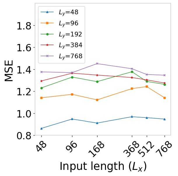
(a) Input length.

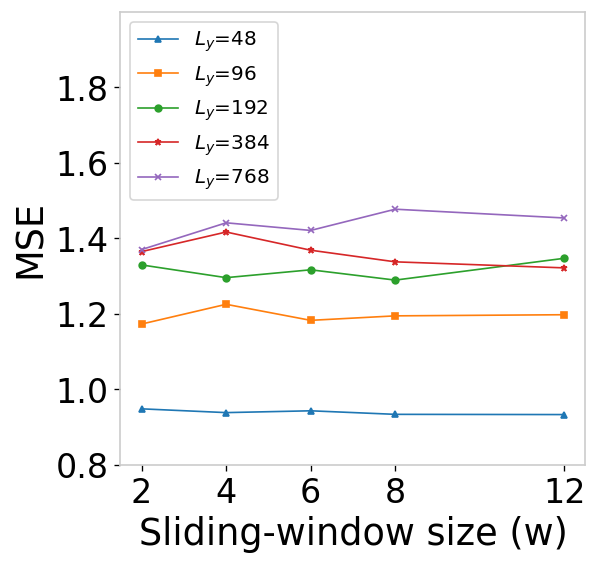
(b) Window size $w$.

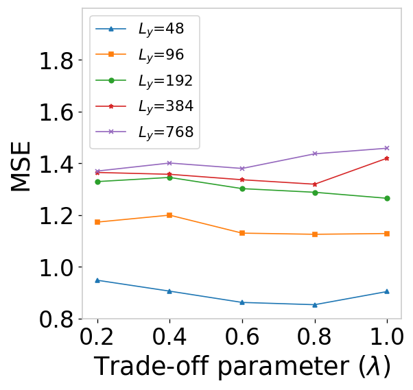
(c) Trade-off parameter $\lambda$.

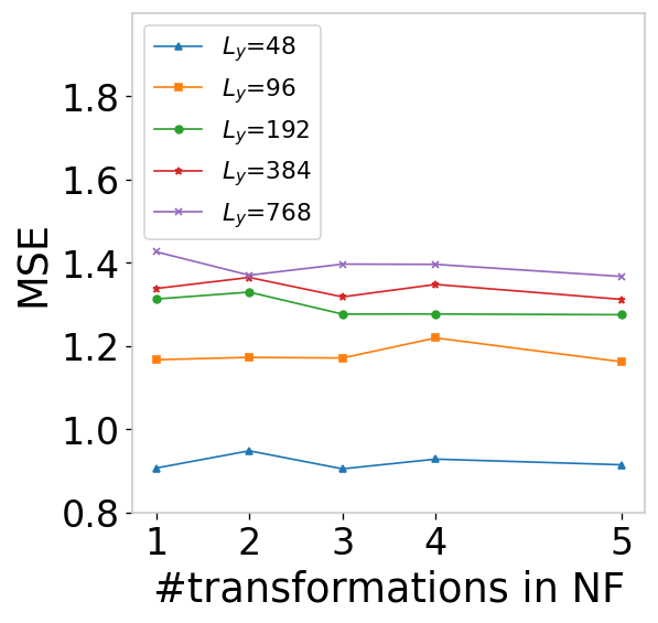
(d) Number of transformations in Normalizing Flow.

Figure 4: Parameter sensitivity analysis of Conformer.

V-D Ablation Study

We conduct the ablation study under multivariate TF setting.

V-D1 Multivariate Correlation and Multiscale Dynamics

We compare Conformer with its tailored variants w.r.t. the multivariate correlation and multiscale dynamics, and report their prediction performances on ECL and ETTm1 datasets. From Table V, we can obtain several insightful clues on how to embed the input series for LTTF. 1) $\mathcal{X}^{in}$ v. $\mathcal{X}^{in}_{-\mathcal{R}}$: Multivariate correlation contributes less when the dimensions of series is higher (#dims. of ECL data is much larger than ETTm1 data) or the predict-length is prolonged. 2) $\mathcal{X}^{in}$ v. $\mathcal{X}^{in}_{-\mathcal{X}-\Gamma}$: Temporal dependency is more important for the series with lower dimensions, and for high dimensional time-series, the effectiveness of temporal dependency can be replaced by the inter-series correlation when $L_{y}$ climbs up. 3) $\mathcal{X}^{in}_{-\mathcal{R}}$ v. $\mathcal{X}^{in}_{-\mathcal{X}}$ and $\mathcal{X}^{in}_{-\mathcal{R}-\Gamma}$ v. $\mathcal{X}^{in}_{-\mathcal{X}-\Gamma}$: Multiscale dynamics delivers better performance when being guided by the raw series, which holds regardless of #dims. of time-series. Besides, multivariate correlation contributes more than the raw data for low dimensional time-series. 4) $\mathcal{X}^{in}_{-\mathcal{R}}$ v. $\mathcal{X}^{in}_{-\mathcal{R}-\Gamma}$ and $\mathcal{X}^{in}_{-\mathcal{X}}$ v. $\mathcal{X}^{in}_{-\mathcal{X}-\Gamma}$: Multiscale dynamics could harm the performance for LTTF when being equipped with the multivariate correlation if the raw time-series is absent.

V-D2 Stationary and Instant Recurrent Network (SIRN)

For the ablation study of the proposed SIRN, we compare Conformer to its different variants by tailoring the encoder-decoder architecture on the Wind dataset, which can be found in Table VI. Specifically, we replace the sliding-window attention and the RNNs with other self-attention mechanisms to verify the effectiveness of SIRN. From Table VI, we can see that SIRN achieves best performance under different settings, which validate the effectiveness of information utilization of combining the local and global patterns.

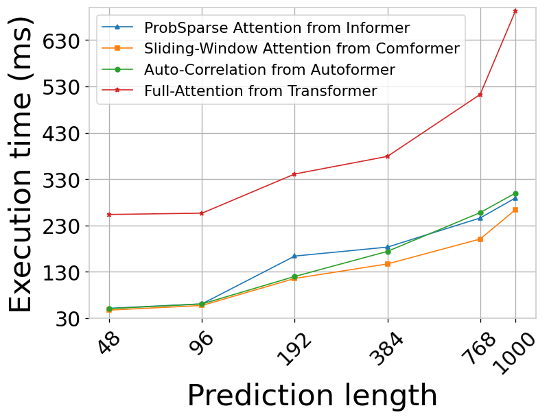
(a) Time complexity.

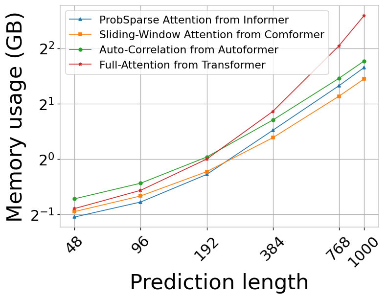
(b) Memory cost.

Figure 5: Computation efficiency analysis. The input length is set as 96 and all the experiments are conducted on the Wind dataset under the multivariate forecasting setting.

V-D3 Normalizing Flow

To verify the effectiveness of normalizing flow block in Conformer for LTTF task, we compare the original Conformer with its several variants. In particular, we tailor the normalizing flow block in Conformer by realizing a generative forecast method with the help of Gaussian probabilistic model as follows:

1. Conformer ${}_{-NF}^{\mathbf{z}_{e}}$: The outcome distribution $\mathbf{z}_{t}$ (yielded by normalizing flow) is replaced by $\mathbf{z}_{e}$ (obtained by Eq. 15).

2. Conformer ${}_{-NF}^{\mathbf{z}_{d}}$: The outcome distribution $\mathbf{z}_{t}$ (yielded by normalizing flow) is replaced by $\mathbf{z}_{d}$. In particular, we replace $\mathbf{h}_{e}$ with $\mathbf{h}_{d}$ in Eq. 15 and generate $\mathbf{z}_{d}$ accordingly.

3. Conformer ${}_{-NF}^{\mathbf{z}_{e}+\mathbf{z}_{d}}$: The outcome distribution $\mathbf{z}_{t}$ (yielded by normalizing flow) is replaced by $\mathbf{z}_{0}$ (obtained by Eq. 16).

4. Conformer _-NF: We implement a tailored Conformer by removing the normalizing flow framework.

The prediction results on Wind dataset are reported in Table VII. We can observe that: 1) The contribution of normalizing flow is indispensable for LTTF regardless of forecast setting and predict length, and 2) the way that we adapt the normalizing flow to the LTTF task is effective.

TABLE VIII: Comparisons of fusing inter-series correlation and time dependency for LTTF.

Dataset		ECL					Exchange
Predict Length		48	96	192	384	768	48	96	192	384
Conformer	MSE	0.1921	0.2124	0.2378	0.2643	0.3396	0.0764	0.1193	0.2900	0.4730
	MAE	0.3034	0.3193	0.3456	0.3620	0.4092	0.2093	0.2607	0.4187	0.5369
Conformer (Method 1)	MSE	0.2003	0.2713	0.2826	0.2898	0.3441	0.1839	0.2938	0.4347	1.0596
	MAE	0.3117	0.3784	0.3790	0.3775	0.4150	0.3371	0.4313	0.5190	0.8072
Conformer (Method 2)	MSE	0.1965	0.2354	0.2632	0.2987	0.3437	0.1593	0.3433	0.4321	0.5486
	MAE	0.3007	0.3323	0.3587	0.3821	0.4191	0.3144	0.4530	0.5197	0.6007
Conformer (Method 3)	MSE	0.1997	0.2791	0.2771	0.3061	0.3433	0.2443	0.3310	0.4089	0.9034
	MAE	0.3117	0.3854	0.3744	0.3881	0.4135	0.3795	0.4597	0.4965	0.7444
Conformer (Method 4)	MSE	0.2010	0.2735	0.2749	0.3078	0.3391	0.1135	0.1534	0.2344	0.5701
	MAE	0.3135	0.3770	0.3710	0.3899	0.4076	0.2597	0.3055	0.3805	0.5978

TABLE IX: Comparisons of feeding hidden states to the normalizing flow block. The best scores are in boldface and the 2nd best scores are in underlines.

Dataset		ECL					Exchange
Predict Length		48	96	192	384	768	48	96	192	384
Conformer	MSE	0.1921	0.2124	0.2378	0.2643	0.3396	0.0764	0.1193	0.2900	0.4730
	MAE	0.3034	0.3193	0.3456	0.3620	0.4092	0.2093	0.2607	0.4187	0.5369
Conformer ($\mathbf{h}^{(e)}_{k}$, $\mathbf{h}^{(d)}_{k}$)	MSE	0.1901	0.2300	0.2814	0.3057	0.3387	0.1150	0.1506	0.2787	0.5593
	MAE	0.3010	0.3322	0.3776	0.3920	0.4168	0.2643	0.3013	0.4108	0.5872
Conformer ($\mathbf{h}^{(e)}_{1}$, $\mathbf{h}^{(d)}_{k}$)	MSE	0.2004	0.2283	0.2554	0.2896	0.3398	0.1156	0.1476	0.2577	0.6053
	MAE	0.3112	0.3321	0.3588	0.3782	0.4121	0.2655	0.2983	0.3911	0.6086
Conformer ($\mathbf{h}^{(e)}_{1}$, $\mathbf{h}^{(d)}_{1}$)	MSE	0.1984	0.2265	0.2507	0.2751	0.3565	0.1181	0.1669	0.2498	0.5300
	MAE	0.3083	0.3304	0.3543	0.3732	0.4226	0.2676	0.3157	0.3925	0.5609
Conformer ($\mathbf{h}^{(e)}_{k}$, $\mathbf{h}^{(d)}_{1}$)	MSE	0.1904	0.2202	0.2512	0.2799	0.3547	0.1155	0.1497	0.2846	0.5203
	MAE	0.3018	0.3260	0.3586	0.3796	0.4259	0.2654	0.3004	0.4140	0.5549

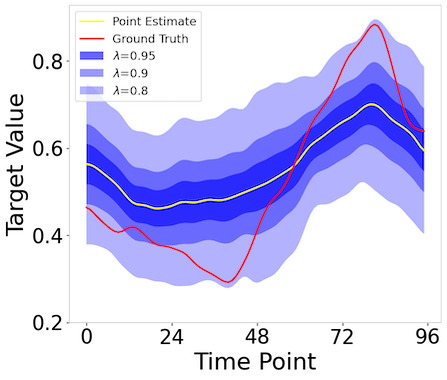
(a) Predict Length = 96.

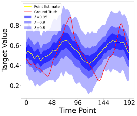
(b) Predict Length = 192.

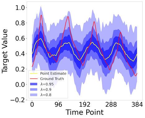
(c) Predict Length = 384.

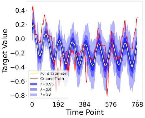
(d) Predict Length = 768.

Figure 6: With the help of Normalizing Flow, Conformer can generate the prediction results with uncertainty quantification for LTTF. Four illustrative cases are demonstrated on the ETTm1 dataset under the multivariate setting. $\lambda$ denotes the contributions of the encoder-decoder, that is, $1-\lambda$ represents the impacts of the normalizing flow block.

V-E Parameter Sensitivity Analysis

We report parameter sensitivity analysis in Fig. 4, which is conducted on the Wind dataset. To be specific, we inspect four hyper parameters including the input length $L_{x}$, the window size $w$ of sliding-window attention, the trade-off parameter $\lambda$ and the number of transformations in Normalizing Flow. Generally, we can observe that the performance of Conformer is quite stable most of the time w.r.t. the varying of different hyper-parameters. In particular, as shown in Fig. 4(a), long-term time-series forecasting setting (e.g., $L_{y}=384$) seems to be more capable of handling longer input, though the volatility of performance is small.

V-F Computational Efficiency Analysis

We conduct execution time consumption and memory usage comparisons between Conformer (with sliding-window attention) and other attention mechanisms. We replace the standard self-attention mechanism in Transformer with different variants and carry out the prediction with the corresponding method for $10^{3}$ times (taking the sequences in different time spans as inputs), then the averaged running time per forecast is reported. For the memory cost comparisons, the maximum memory usage is recorded. The time consumption and memory usage of different attentions are demonstrated in Fig. 5. Conformer performs with better efficiency in both short- and long-term time-series forecasting.

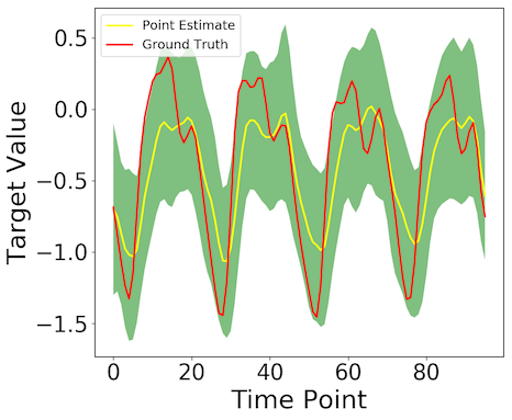
(a) #transformations = 1.

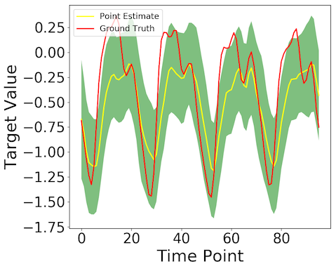
(b) #transformations = 2.

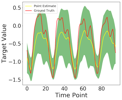
(c) #transformations = 3.

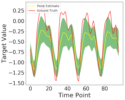
(d) #transformations = 4.

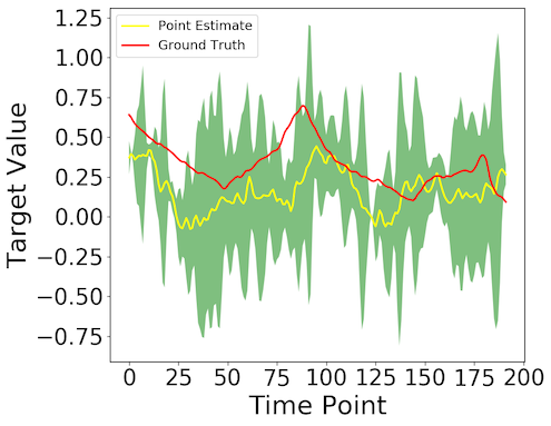
(e) #transformations = 1.

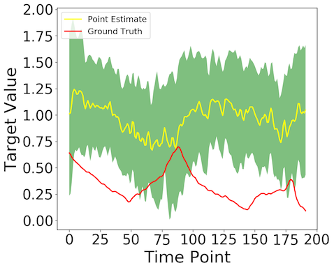
(f) #transformations = 2.

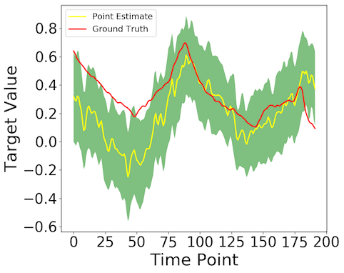
(g) #transformations = 3.

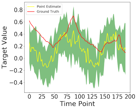
(h) #transformations = 4.

Figure 7: Uncertainty-aware LTTF with varying #transforms. To evaluate the performance of normalizing flow more clearly, we omit the contribution of SIRN by setting $\lambda=0$ in Eq. 18. (a)–(d) and (e)–(h) demonstrate two cases in ECL and ETTm1 datasets, respectively.

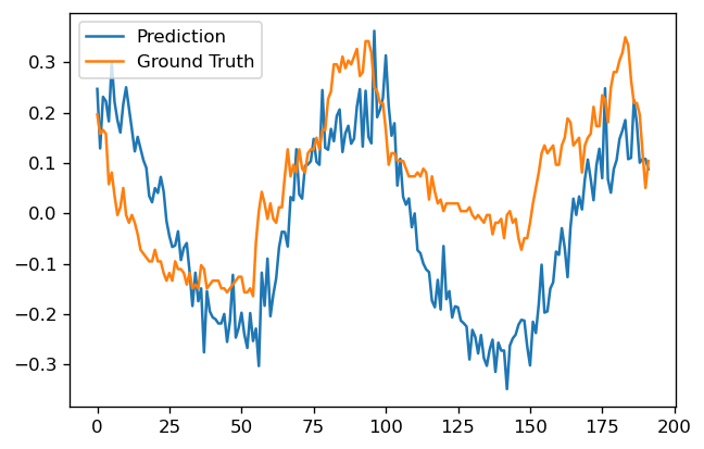
(a) Conformer

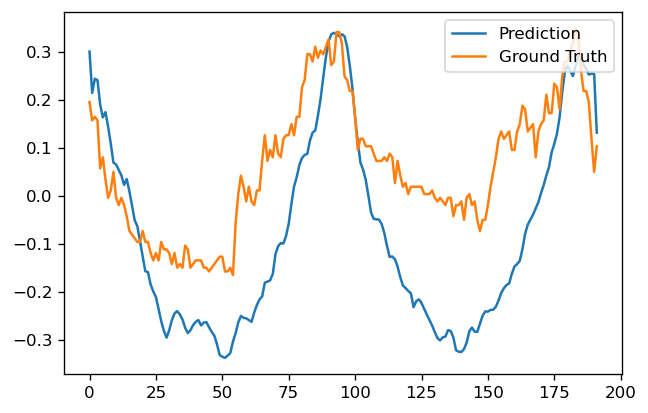
(b) Longformer

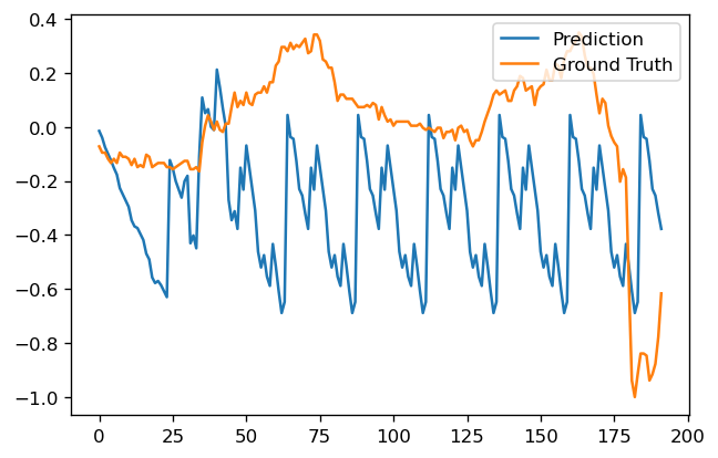
(c) Reformer

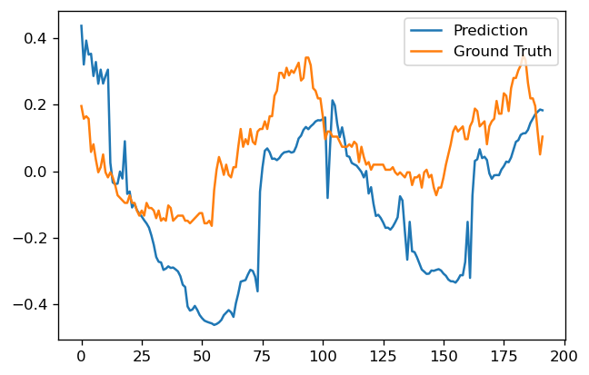
(d) Informer

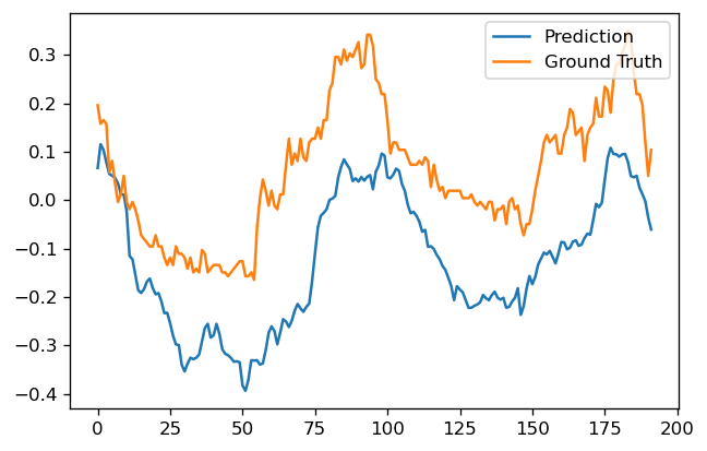
(e) Autoformer

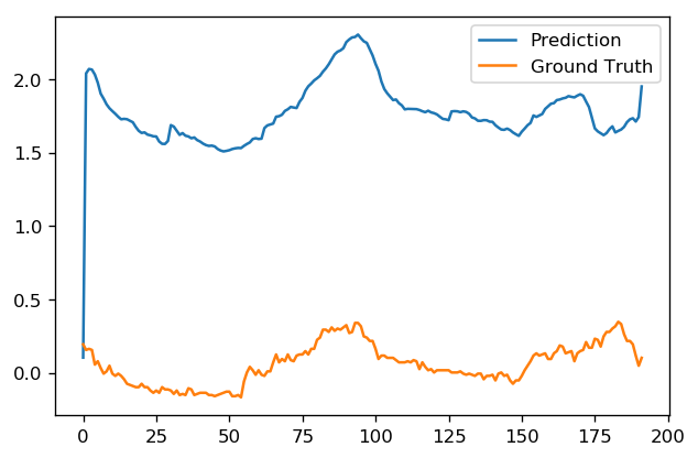
(f) N-Beats

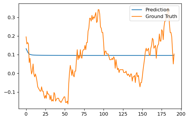
(g) LSTNet

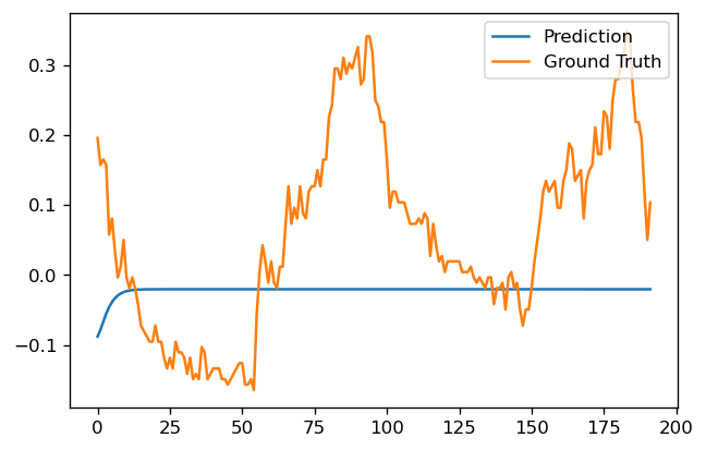
(h) GRU

Figure 8: Prediction cases on the ETTm1 dataset under the input-96-predict-192 setting.

V-G Model Analysis

V-G1 Fusing Inter-Series and Across-Time Dependencies

As introduced in Section IV-A, the series data is embedded and fused by taking the multivariate correlation and multiscale dynamics into account. To further assess the effectiveness of input representation module in Conformer, we realize different ways of fusing multivariate correlation and multiscale dynamics below (let $\mathbf{W}^{\Gamma}=\text{Softmax}(\bar{\Gamma}^{S})$):

1. Method 1: $\mathcal{X}^{in}=\mathbf{W}^{v}\odot(\mathbf{W}^{\Gamma}\mathbf{W}^{\mathcal{R}}\mathcal{X}+\mathcal{X})+\mathbf{b}^{v}$

2. Method 2: $\mathcal{X}^{in}=\mathbf{W}^{v}\odot(\mathbf{W}^{\mathcal{R}}\mathcal{X}+\mathbf{W}^{\Gamma}\mathcal{X})+\mathbf{b}^{v}$

3. Method 3: $\mathcal{X}^{in}=\mathbf{W}^{v}\odot(\mathbf{W}^{\mathcal{R}}\mathcal{X}+\mathbf{W}^{\Gamma}\mathcal{X}+\mathcal{X})+\mathbf{b}^{v}$

4. Method 4: $\mathcal{X}^{in}=[\mathbf{W}^{v}\odot(\mathbf{W}^{\mathcal{R}}\mathcal{X}+\mathcal{X})+\mathbf{b}^{v}]\mathbf{W}^{\Gamma}$

The results are reported in Table VIII. We can see that how to fuse the multivariate correlation and temporal dependency is important for the LTTF task. This impact weighs more for low dimensional time-series data since the self-attention mechanism in encoder-decoder architecture can better explore intricate dependencies when the dimensionality grows.

V-G2 Uncertainty-Aware Forecasting

The outcome variance of the Normalizing Flow block can suggest the fluctuation range of the forecasting results. We randomly select a case in ETTm1 dataset under the multivariate setting and demonstrate the forecasting results with uncertainty quantification for different output lengths in Fig. 6. We can see that Conformer tends to make a conservative forecast and the uncertainty quantification can cover the extreme ground truth values if the NF block can be weighted more.

V-G3 How Far The Message Should Be Cascaded in Normalizing Flow

We inspect how the normalizing flow works for LTTF by varying the number of transformations on two cases in ECL and ETTm1 datasets, respectively, in Fig. 7. We can see that the further the latent variable being transformed the better the outcome series performs. Therefore, the power of normalizing flow in Conformer for LTTF should be explored more dedicatedly.

V-G4 How to Feed Hidden States to The Normalizing Flow Block in Conformer

As shown in Fig. 1, in both encoder and decoder, the first outcome hidden state of the last SIRN layer is fed to the normalizing flow. To assess the effect of feeding hidden states to normalizing flow, we implement Conformer by combining the outcome hidden states in the first/last SIRN layer of the encoder/decoder, which results in Conformer ($\mathbf{h}^{(e)}_{k}$, $\mathbf{h}^{(d)}_{k}$), Conformer ($\mathbf{h}^{(e)}_{1}$, $\mathbf{h}^{(d)}_{k}$), Conformer ($\mathbf{h}^{(e)}_{1}$, $\mathbf{h}^{(d)}_{1}$) and Conformer ($\mathbf{h}^{(e)}_{k}$, $\mathbf{h}^{(d)}_{1}$) where $k$ denotes the last SIRN layer. We report the prediction results in Table IX. As can be seen, the impact of feeding different hidden states to normalizing flow is generally marginal though, the low dimensional time-series forecasting is more sensitive to the way of absorbing hidden states for normalizing flow.

V-H Multivariate Time-series Forecasting Showcase

We additionally plot the prediction and the ground truth of the target value. The qualitative comparisons between Conformer and other baselines on ETTm1 dataset are demonstrated in Fig. 8. We can see that, our model obviously achieves the best performance among different methods.

V-I Discussion

Windowed Attention: Conformer v. Swin Transformer. The windowed attention mechanism is applied in many applications thanks to its linear complexity, such that the powerful self-attention can be scaled up to large data. The very recent Swin Transformer [50] and its variant [51] adopt the windowed attention and devise a shifted window attention to implement a general purpose backbone for computer vision tasks. Basically, both Conformer and Swin Transformer exploit the self-attention within neighbored/partitioned windows regarding the computational efficiency. Besides the locality, connectivity is another merit one can not neglect. To achieve connectivity, a shifted window mechanism is proposed for Swin Transformer, while we propose SIRN for Conformer so as to absorb long-range dependencies in the time-series data. 

Comparisons of Computational Complexity. The windowed attention contributes most to the complexity reduction of Conformer. Hence, we take different SOTA attention mechanisms as competitors to conduct the computational complexity analysis in Section V-F. The computational costs of other components in Conformer are not elaborated, which will be provided in our future work.

VI Conclusion

In this paper, we proposed a transformer-based model, namely Conformer, to address the long-term time-series forecasting (LTTF) problem. Specifically, Conformer first embeds the input time series with the multivariate correlation modeling and multiscale dynamics extraction to fuel the downstream self-attention mechanism. Then, to reduce the computation complexity of self-attention and fully distill the series-level temporal dependencies without sacrificing information utilization for LTTF, sliding-window attention, as well as a proposed stationary and instant recurrent network (SIRN), are equipped to the Conformer. Moreover, a normalizing flow framework is employed to further absorb the latent states in the SIRN, such that the underlying distribution can be learned and the target series can be directly reconstructed in a generative way. Extensive empirical studies on six real-world datasets validate that Conformer achieves state-of-the-art performance on long-term time-series forecasting under multivariate and univariate prediction settings. In addition, with the help of normalizing flow, Conformer can generate the prediction results with uncertainty quantification.

References

- [1] G. Lai, W.-C. Chang, Y. Yang, and H. Liu, “Modeling long-and short-term temporal patterns with deep neural networks,” in The 41st International ACM SIGIR Conference on Research & Development in Information Retrieval, 2018, pp. 95–104.
- [2] Y. Wang, R. Zou, F. Liu, L. Zhang, and Q. Liu, “A review of wind speed and wind power forecasting with deep neural networks,” Applied Energy, vol. 304, p. 117766, 2021.
- [3] J. Han, H. Liu, H. Zhu, H. Xiong, and D. Dou, “Joint air quality and weather prediction based on multi-adversarial spatiotemporal networks,” in Proceedings of the 35th AAAI Conference on Artificial Intelligence, 2021.
- [4] Y. Matsubara, Y. Sakurai, W. G. Van Panhuis, and C. Faloutsos, “Funnel: automatic mining of spatially coevolving epidemics,” in Proceedings of the 20th ACM SIGKDD international conference on Knowledge discovery and data mining, 2014, pp. 105–114.
- [5] A. A. Ariyo, A. O. Adewumi, and C. K. Ayo, “Stock price prediction using the arima model,” in 2014 UKSim-AMSS 16th International Conference on Computer Modelling and Simulation. IEEE, 2014, pp. 106–112.
- [6] K. Gregor, I. Danihelka, A. Mnih, C. Blundell, and D. Wierstra, “Deep autoregressive networks,” in International Conference on Machine Learning. PMLR, 2014, pp. 1242–1250.
- [7] I. Melnyk and A. Banerjee, “Estimating structured vector autoregressive models,” in International Conference on Machine Learning. PMLR, 2016, pp. 830–839.
- [8] K.-j. Kim, “Financial time series forecasting using support vector machines,” Neurocomputing, vol. 55, no. 1-2, pp. 307–319, 2003.
- [9] D. Salinas, V. Flunkert, J. Gasthaus, and T. Januschowski, “Deepar: Probabilistic forecasting with autoregressive recurrent networks,” International Journal of Forecasting, vol. 36, no. 3, pp. 1181–1191, 2020.
- [10] A. Graves, “Generating sequences with recurrent neural networks,” arXiv preprint arXiv:1308.0850, 2013.
- [11] I. Sutskever, O. Vinyals, and Q. V. Le, “Sequence to sequence learning with neural networks,” in Advances in neural information processing systems, 2014, pp. 3104–3112.
- [12] N. Kitaev, Ł. Kaiser, and A. Levskaya, “Reformer: The efficient transformer,” arXiv preprint arXiv:2001.04451, 2020.
- [13] J. Xu, J. Wang, M. Long et al., “Autoformer: Decomposition transformers with auto-correlation for long-term series forecasting,” Advances in Neural Information Processing Systems, vol. 34, 2021.
- [14] S. Li, X. Jin, Y. Xuan, X. Zhou, W. Chen, Y. Wang, and X. Yan, “Enhancing the locality and breaking the memory bottleneck of transformer on time series forecasting,” CoRR, vol. abs/1907.00235, 2019. [Online]. Available: http://arxiv.org/abs/1907.00235
- [15] H. Zhou, S. Zhang, J. Peng, S. Zhang, J. Li, H. Xiong, and W. Zhang, “Informer: Beyond efficient transformer for long sequence time-series forecasting,” in Proceedings of the AAAI Conference on Artificial Intelligence, vol. 35, no. 12, 2021, pp. 11 106–11 115.
- [16] I. Beltagy, M. E. Peters, and A. Cohan, “Longformer: The long-document transformer,” CoRR, vol. abs/2004.05150, 2020. [Online]. Available: https://arxiv.org/abs/2004.05150
- [17] M. Zaheer, G. Guruganesh, A. Dubey, J. Ainslie, C. Alberti, S. Ontañón, P. Pham, A. Ravula, Q. Wang, L. Yang, and A. Ahmed, “Big bird: Transformers for longer sequences,” CoRR, vol. abs/2007.14062, 2020. [Online]. Available: https://arxiv.org/abs/2007.14062
- [18] J. Gawlikowski, C. R. N. Tassi, M. Ali, J. Lee, M. Humt, J. Feng, A. Kruspe, R. Triebel, P. Jung, R. Roscher et al., “A survey of uncertainty in deep neural networks,” arXiv preprint arXiv:2107.03342, 2021.
- [19] L.-J. Cao and F. E. H. Tay, “Support vector machine with adaptive parameters in financial time series forecasting,” IEEE Transactions on neural networks, vol. 14, no. 6, pp. 1506–1518, 2003.
- [20] S. Hochreiter and J. Schmidhuber, “Long short-term memory,” Neural computation, vol. 9, no. 8, pp. 1735–1780, 1997.
- [21] R. Dey and F. M. Salem, “Gate-variants of gated recurrent unit (gru) neural networks,” in 2017 IEEE 60th international midwest symposium on circuits and systems (MWSCAS). IEEE, 2017, pp. 1597–1600.
- [22] A. Borovykh, S. Bohte, and C. W. Oosterlee, “Conditional time series forecasting with convolutional neural networks,” arXiv preprint arXiv:1703.04691, 2017.
- [23] R. Mittelman, “Time-series modeling with undecimated fully convolutional neural networks,” arXiv preprint arXiv:1508.00317, 2015.
- [24] A. Borovykh, S. Bohte, and C. W. Oosterlee, “Dilated convolutional neural networks for time series forecasting,” Journal of Computational Finance, Forthcoming, 2018.
- [25] M. Benhaddi and J. Ouarzazi, “Multivariate time series forecasting with dilated residual convolutional neural networks for urban air quality prediction,” Arabian Journal for Science and Engineering, vol. 46, no. 4, pp. 3423–3442, 2021.
- [26] A. Vaswani, N. Shazeer, N. Parmar, J. Uszkoreit, L. Jones, A. N. Gomez, L. Kaiser, and I. Polosukhin, “Attention is all you need,” CoRR, vol. abs/1706.03762, 2017. [Online]. Available: http://arxiv.org/abs/1706.03762
- [27] R. Child, S. Gray, A. Radford, and I. Sutskever, “Generating long sequences with sparse transformers,” CoRR, vol. abs/1904.10509, 2019. [Online]. Available: http://arxiv.org/abs/1904.10509
- [28] D. A. Reynolds, “Gaussian mixture models.” Encyclopedia of biometrics, vol. 741, pp. 659–663, 2009.
- [29] Y. Wu, J. Ni, W. Cheng, B. Zong, D. Song, Z. Chen, Y. Liu, X. Zhang, H. Chen, and S. Davidson, “Dynamic gaussian mixture based deep generative model for robust forecasting on sparse multivariate time series,” arXiv preprint arXiv:2103.02164, 2021.
- [30] S. S. Rangapuram, L. D. Werner, K. Benidis, P. Mercado, J. Gasthaus, and T. Januschowski, “End-to-end learning of coherent probabilistic forecasts for hierarchical time series,” in Proceedings of the 38th International Conference on Machine Learning, ser. Proceedings of Machine Learning Research, M. Meila and T. Zhang, Eds., vol. 139. PMLR, 18–24 Jul 2021, pp. 8832–8843. [Online]. Available: https://proceedings.mlr.press/v139/rangapuram21a.html
- [31] K. Rasul, C. Seward, I. Schuster, and R. Vollgraf, “Autoregressive denoising diffusion models for multivariate probabilistic time series forecasting,” CoRR, vol. abs/2101.12072, 2021. [Online]. Available: https://arxiv.org/abs/2101.12072
- [32] I. Kobyzev, S. Prince, and M. Brubaker, “Normalizing flows: An introduction and review of current methods,” IEEE Transactions on Pattern Analysis and Machine Intelligence, 2020.
- [33] I. Goodfellow, J. Pouget-Abadie, M. Mirza, B. Xu, D. Warde-Farley, S. Ozair, A. Courville, and Y. Bengio, “Generative adversarial nets,” Advances in neural information processing systems, vol. 27, 2014.
- [34] D. P. Kingma and M. Welling, “Auto-encoding variational bayes,” arXiv preprint arXiv:1312.6114, 2013.
- [35] H. J. Nussbaumer, “The fast fourier transform,” in Fast Fourier Transform and Convolution Algorithms. Springer, 1981, pp. 80–111.
- [36] W. T. Cochran, J. W. Cooley, D. L. Favin, H. D. Helms, R. A. Kaenel, W. W. Lang, G. C. Maling, D. E. Nelson, C. M. Rader, and P. D. Welch, “What is the fast fourier transform?” Proceedings of the IEEE, vol. 55, no. 10, pp. 1664–1674, 1967.
- [37] H. Musbah, M. El-Hawary, and H. Aly, “Identifying seasonality in time series by applying fast fourier transform,” in 2019 IEEE Electrical Power and Energy Conference (EPEC), 2019, pp. 1–4.
- [38] G. E. Box, G. M. Jenkins, G. C. Reinsel, and G. M. Ljung, Time series analysis: forecasting and control. John Wiley & Sons, 2015.
- [39] M. Zaheer, A. Ahmed, and A. J. Smola, “Latent lstm allocation: Joint clustering and non-linear dynamic modeling of sequence data,” in International Conference on Machine Learning. PMLR, 2017, pp. 3967–3976.
- [40] O. Kovaleva, A. Romanov, A. Rogers, and A. Rumshisky, “Revealing the dark secrets of BERT,” CoRR, vol. abs/1908.08593, 2019. [Online]. Available: http://arxiv.org/abs/1908.08593
- [41] K. Cho, B. Van Merriënboer, C. Gulcehre, D. Bahdanau, F. Bougares, H. Schwenk, and Y. Bengio, “Learning phrase representations using rnn encoder-decoder for statistical machine translation,” arXiv preprint arXiv:1406.1078, 2014.
- [42] Y. Luo, Z. Chen, and T. Yoshioka, “Dual-path rnn: efficient long sequence modeling for time-domain single-channel speech separation,” in ICASSP 2020-2020 IEEE International Conference on Acoustics, Speech and Signal Processing (ICASSP). IEEE, 2020, pp. 46–50.
- [43] F. Wang, Z. Xuan, Z. Zhen, K. Li, T. Wang, and M. Shi, “A day-ahead pv power forecasting method based on lstm-rnn model and time correlation modification under partial daily pattern prediction framework,” Energy Conversion and Management, vol. 212, p. 112766, 2020.
- [44] M. Monti, J. Fiorentino, E. Milanetti, G. Gosti, and G. G. Tartaglia, “Prediction of time series gene expression and structural analysis of gene regulatory networks using recurrent neural networks,” Entropy, vol. 24, no. 2, p. 141, 2022.
- [45] C. Robert, C. William, and T. Irma, “Stl: A seasonal-trend decomposition procedure based on loess,” Journal of official statistics, vol. 6, no. 1, pp. 3–73, 1990.
- [46] N. Nguyen and B. Quanz, “Temporal latent auto-encoder: A method for probabilistic multivariate time series forecasting,” in Proceedings of the AAAI Conference on Artificial Intelligence, vol. 35, no. 10, 2021, pp. 9117–9125.
- [47] D. P. Kingma, T. Salimans, R. Jozefowicz, X. Chen, I. Sutskever, and M. Welling, “Improved variational inference with inverse autoregressive flow,” Advances in neural information processing systems, vol. 29, pp. 4743–4751, 2016.
- [48] B. N. Oreshkin, D. Carpov, N. Chapados, and Y. Bengio, “N-beats: Neural basis expansion analysis for interpretable time series forecasting,” in International Conference on Learning Representations, 2019.
- [49] Z. Yue, Y. Wang, J. Duan, T. Yang, C. Huang, Y. Tong, and B. Xu, “Ts2vec: Towards universal representation of time series,” in Proceedings of the AAAI Conference on Artificial Intelligence, vol. 36, no. 8, 2022, pp. 8980–8987.
- [50] Z. Liu, Y. Lin, Y. Cao, H. Hu, Y. Wei, Z. Zhang, S. Lin, and B. Guo, “Swin transformer: Hierarchical vision transformer using shifted windows,” in Proceedings of the IEEE/CVF International Conference on Computer Vision (ICCV), 2021.
- [51] Z. Liu, H. Hu, Y. Lin, Z. Yao, Z. Xie, Y. Wei, J. Ning, Y. Cao, Z. Zhang, L. Dong, F. Wei, and B. Guo, “Swin transformer v2: Scaling up capacity and resolution,” in International Conference on Computer Vision and Pattern Recognition (CVPR), 2022.