An Automatic Method for Generating Symbolic Expressions of Zernike Circular Polynomials

Abstract

Zernike circular polynomials (ZCP) play a significant role in optics engineering. The symbolic expressions for ZCP are valuable for theoretic analysis and engineering designs. However, there are still two problems which remain open: firstly, there is a lack of sufficient mathematical formulas of the ZCP for optics designers; secondly the formulas for inter-conversion of Noll’s single index and Born-Wolf’s double indices of ZCP are neither uniquely determinate nor satisfactory. An automatic method for generating symbolic expressions for ZCP is proposed based on five essential factors: the new theorems for converting the single/double indices of the ZCP, the robust and effective numeric algorithms for computing key parameters of ZCP, the symbolic algorithms for generating mathematical expressions of ZCP, and meta-programming & LaTeX programming for generating the table of ZCP. The theorems, method, algorithms and system architecture proposed are beneficial to both optics design process, optics software, computer-output typesetting in publishing industry as well as STEM education.
Keywords: Zernike circular polynomial, Symbolic computation, Mathematical table, Computer-output typesetting, LaTeX programming, STEM education

1 Introduction

In optics engineering, the Zernike circular polynomials (ZCP), also named Zernike polynomials for simplicity, are essential for representing aberrations in imaging system, optics design and optical testing [1, 2, 3, 4, 5, 6, 7, 8, 9]. Mathematically, ZCP are a sequence of bivariate polynomials defined on the unit disk

$$\mathcal{D} =\left\{(x,y):0\leq x^{2}+y^{2}\leq 1\right\}$$

$$=\left\{(\rho,\theta):0\leq\rho\leq 1,0\leq\theta\leq 2\pi\right\}$$

derived from the circular pupils of imaging system. Named after Frits Zernike, they play an important role in beam optics and optics design[10], atmospheric turbulence [11] and image processing [12]. The ZCP are orthogonal functions which represent balanced aberrations that yield minimum variance[9]. The computation of ZCP are significant for theoretic analysis and engineering applications. The numerical algorithms are discussed in lots of literature such as [4, 13, 12, 14]. However, the symbolic computation for automatically generating the mathematical expressions for the ZCP is missing. It may be inconvenient or troublesome for the optics designers to look for the formulas of ZCP with ”high” orders. Actually, there are less $28\sim 40$ and $70$ expressions for the ZCP in ZEMAX and CodeV respectively.

The purpose of this paper is to propose an automatic method for generating mathematical expressions for the ZCP. FIGURE 1 illustrates the framework of our work. There are five modules for the system architecture:

• Principle of Index Conversion, which includes our new theorems and proofs about the single/double index for the ZCP;

• Numeric computation, which computes key parameters robustly and effectively for large integers so as to avoid the overflow problem in computing factorials;

• Symbolic computation, which deals with the algorithms for automatic generating symbolic expressions of the ZCP;

• Meta-programming and LaTeX programming, which generates the long table of ZCP and outputs the corresponding pdf file for printing, reading and reference;

• System setting, which sets the necessary information for the mathematical formula of ZCP and the geometric configuration of the long table of mathematical expressions.

The contents of this paper are organized as follows: Section 2 deals with the preliminaries of backgrounds; Section 3 copes with the principle of inter-conversion of the single/double index for computing ZCP; Section 4 focuses on how to generate long table of mathematical expressions of ZCP; Section 5 is the conclusion.

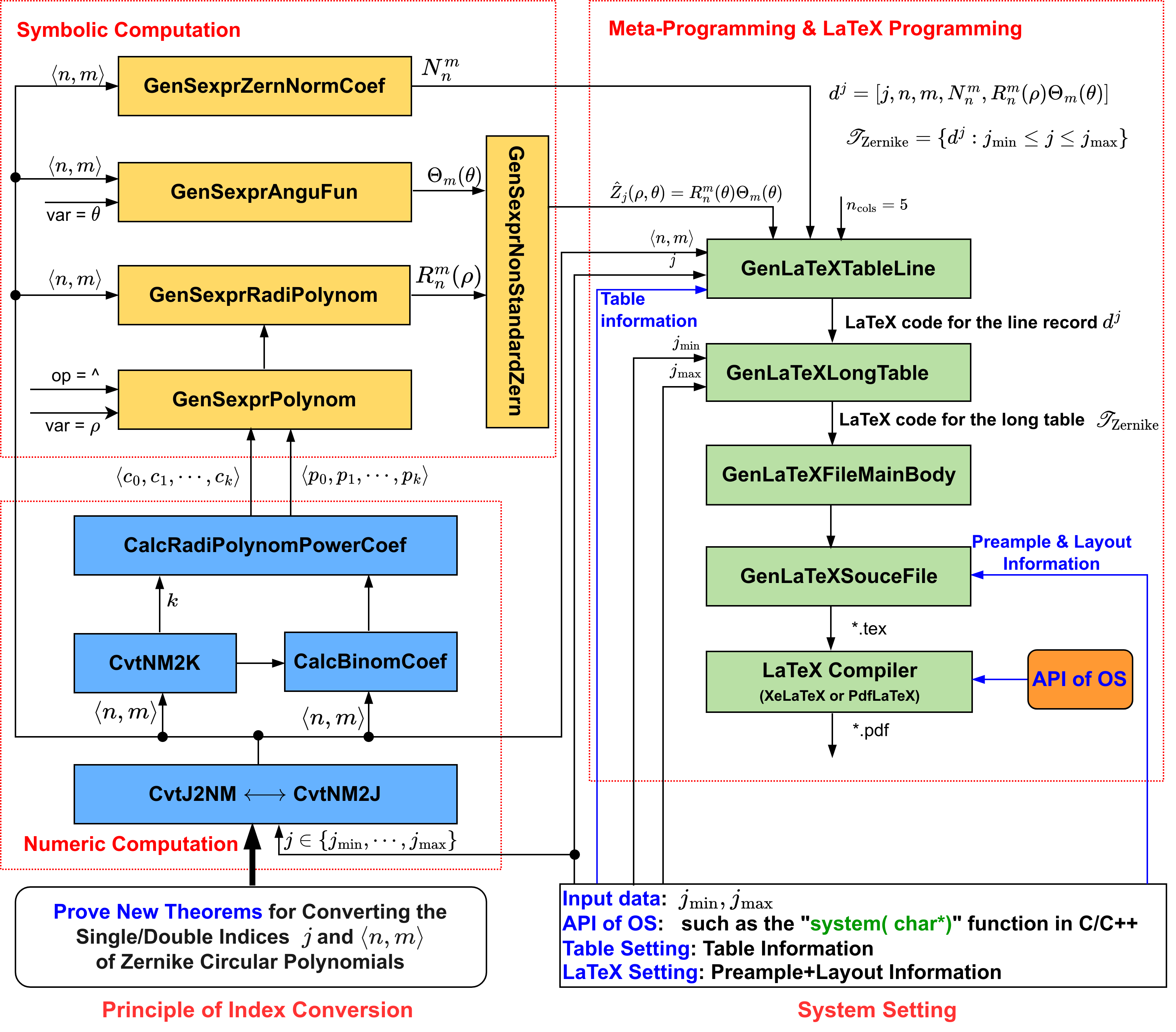
Figure 1: System architecture for automatically generating a long table of the mathematical expressions of ZCP $\left\{\operatorname{Z}_{j}(\rho,\theta):{j}_{\mathrm{min}}\leq j\leq{j}_{\mathrm{max}}\right\}$

2 Preliminaries

2.1 Fundamentals of Mathematics

2.1.1 Notations for Integers

For an integer $n\in\mathbb{Z}=\left\{0,\pm 1,\pm 2,\cdots\right\}$, it is even if and only if $2\mid n$, i.e., $2$ divides $n$ or equivalently $n\equiv 0\leavevmode\nobreak\ (\operatorname{mod}2)$; otherwise, it is odd if and only if $2\nmid n$ or equivalently $n\equiv 1\leavevmode\nobreak\ (\operatorname{mod}2)$. The sets of even and odd integers are denoted by

$$\mathbb{Z}_{\mathrm{odd}}=\left\{i\in\mathbb{Z}:2\nmid i\right\}=\left\{\pm 1,\pm 3,\pm 5,\cdots\right\}$$

and

$$\mathbb{Z}_{\mathrm{even}}=\left\{i\in\mathbb{Z}:2\mid i\right\}=\left\{0,\pm 2,\pm 4,\pm 6,\cdots\right\}$$

respectively. The set of positive integers are $\mathbb{N}=\left\{1,2,3,\cdots\right\}$ and the set of non-negative integers is $\mathbb{Z}^{+}=\mathbb{N}\cup\left\{0\right\}=\left\{0,1,2,\cdots\right\}$. Similarly, the set of negative integers is $\mathbb{Z}^{-}=-\mathbb{N}=\left\{-1,-2,-3,\cdots\right\}$. In consequence, the sets of non-negative even integers and non-negative odd integers can be denoted by ${\mathbb{Z}}_{\mathrm{even}}^{+}$ and ${\mathbb{Z}}_{\mathrm{odd}}^{+}$ respectively.

For any real number $x\in\mathbb{R}$, the unique integer $n=\left\lfloor{x}\right\rfloor\in\mathbb{Z}$ such that $n\leq x<n+1$ is called the floor of $x$. Similarly, the integer $n^{\prime}=\left\lceil{x}\right\rceil\in\mathbb{Z}$ such that $n^{\prime}-1<x\leq n^{\prime}$ is called the ceiling of $x$.

2.1.2 Expression of General Polynomials

A polynomial $T_{n}(x)$ with argument $x$ and degree $n$ can be written by

$$T_{n}(x)=\sum^{n}_{i=0}a_{i}x^{i}=a_{0}+a_{1}x+\cdots+a_{i}x^{i}+\cdots+a_{n}x^{n}$$ (1)

If $a_{i}=0$ for all odd $i$ , then $T_{n}(x)$ is an even polynomial. Similarly, if $a_{i}=0$ for all even $i$, then $T_{n}(x)$ is an odd polynomial. Futhermore, some of the coefficients $a_{0},a_{1},\cdots,a_{n}$ may be missing if they equal zero. In consequence, we can denote a polynomial as

$$T(x)=\sum^{k}_{s=0}c_{s}x^{p_{s}},\quad p_{s}\in\mathbb{Z}^{+}$$ (2)

where $p_{s}\in\mathbb{Z}^{+}$. In other words, a polynomial can be described by the sequence of coefficients $\texttt{c}=\langle c_{0},\cdots,c_{k}\rangle$ and the corresponding sequence of power indices $\texttt{p}=\langle p_{0},\cdots,p_{k}\rangle$.

2.1.3 Binomial and Tri-nomial Coefficients

In general, for any real number $\alpha\in\mathbb{R}$ and non-negative $i\in\mathbb{Z}^{+}=\left\{0,1,2,\cdots\right\}$ the generalized binomial expansion can be expressed by

$$(1+x)^{\alpha}=\sum^{\infty}_{i=0}\binom{\alpha}{i}x^{i},\quad x\in\mathrm{ROC}=(-1,1)$$

in which ROC is the region of convergence and

$$\binom{\alpha}{i}=\frac{\alpha(\alpha-1)\cdots(\alpha-i+1)}{i!}$$ (3)

is the binomial coefficient [15, 16, 17]. Particularly, if $\alpha\in\mathbb{Z}^{+}$ is a positive integer, we have

$$\binom{\alpha}{i}=\frac{\alpha!}{i!(\alpha-i)!}.$$ (4)

For any $r\in\mathbb{Z}^{+}$ we have

$$(x_{1}+x_{2}+x_{3})^{r}=\sum_{i_{1}+i_{2}+i_{3}=r}\binom{r}{i_{1},i_{2},i_{3}}x^{i_{1}}_{1}x^{i_{2}}_{2}x^{i_{3}}_{3}$$

where

$$\binom{r}{i_{1},i_{2},i_{3}}=\frac{(i_{1}+i_{2}+i_{3})!}{i_{1}!i_{2}!i_{3}!},\quad i_{1}+i_{2}+i_{3}=r$$ (5)

is the tri-nomial coefficients, which is symmetric for a permutation of $i_{1},i_{2},i_{3}$ and can be expressed in terms of binomial coefficients:

$$\binom{r}{i_{1},i_{2},i_{3}}=\binom{i_{1}+i_{2}}{i_{1}}\binom{i_{1}+i_{2}+i_{3}}{i_{1}+i_{2}}.$$ (6)

Therefore, for $r=n-s,p=3,i_{1}=s,i_{2}=k-s,i_{3}=n-k-s,i_{1}+i_{2}+i_{3}=n-s$, we can obtain

$$\binom{n-s}{s,k-s,n-k-s}=\binom{k}{s}\binom{n-s}{k}.$$ (7)

When computing the value of binomial coefficients with computer programs, we should keep an eye on the overflow problem since the factorial $r!$ increases rapidly with the integer $r$. We can avoid such a risk by reformulating the binomial coefficient properly, i.e., for any $i\in\mathbb{Z}=\left\{0\right\}\cup\mathbb{N}$,

$$\binom{\alpha}{i}=\left\{\begin{array}[]{ll}1,&i=0;\\ \prod\limits^{i-1}_{t=0}\cfrac{\alpha-t}{i-t},&i\geq 1.\end{array}\right.$$ (8)

The value of $\binom{\alpha}{i}$ can be computed with Algorithm 4.1.3 robustly and fastly.

2.1.4 Kronecker Symbol

The notation

$$\delta_{ij}=\left\{\begin{array}[]{ll}0,&i\neq j\\ 1,&i=j\end{array}\right.$$ (9)

is called the Kronecker symbol. Particularly, $\delta_{m0}=1$ for $m=0$ and $\delta_{m0}=0$ otherwise.

2.1.5 Discrete Unit Step Function

The discrete unit step function is defined by

$$u(m)=\left\{\begin{array}[]{ll}1,&m\in\mathbb{Z}^{+}=\left\{0,1,2,3,\cdots\right\}\\ 0,&m\in\mathbb{Z}^{-}=\left\{-1,-2,-3,\cdots\right\}\end{array}\right.$$ (10)

with the counterpart of Heaviside function in the continuous case.

2.1.6 Cardinality

For a finite set $A=\left\{x_{1},\cdots,x_{r}\right\}$, its cardinality is denoted by $\left|A\right|$, i.e.

$$\left|A\right|=\left|\left\{x_{1},\cdots,x_{r}\right\}\right|=r.$$ (11)

2.2 Zernike Circular Polynomials

2.2.1 Definition of Zernike Circular Polynomials

Generally, for $n\in\mathbb{Z}^{+}$ and $m\in\mathbb{Z}$ such that $\left|m\right|\leq n$ and $2\mid(n-m)$, the ZCP can be denoted by [1, 3, 4]

$$\operatorname{Z}_{n}^{m}(\rho,\theta)=N^{m}_{n}\operatorname{R}_{n}^{m}(\rho)\Theta_{m}(\theta),\quad\rho\in[0,1],\theta\in[0,2\pi]$$ (12)

where

$$N^{m}_{n}=\sqrt{\frac{2(n+1)}{1+\delta_{m0}}}=\left\{\begin{array}[]{ll}\sqrt{2(n+1)},&m\neq 0\\ \sqrt{n+1},&m=0\end{array}\right.$$ (13)

is the coefficients for normalization,

$$\Theta_{m}(\theta)=\left\{\begin{array}[]{ll}1,&m=0,j\in{\mathbb{Z}}_{\mathrm{odd}}^{+}\\ \cos(\left|m\right|\theta),&m\neq 0,j\in{\mathbb{Z}}_{\mathrm{even}}^{+}\\ \sin(\left|m\right|\theta),&m\neq 0,j\in{\mathbb{Z}}_{\mathrm{odd}}^{+}\end{array}\right.$$ (14)

is the angular function with equivalent complex form $\mathrm{e}^{\mathrm{i}\left|m\right|\theta}$,

$$\begin{split}\operatorname{R}_{n}^{m}(\rho)&=\frac{1}{(\frac{n-\left|m\right|}{2})!\rho^{\left|m\right|}}\left[\frac{\operatorname{d}}{\operatorname{d}(\rho^{2})}\right]^{\frac{n-\left|m\right|}{2}}\left[(\rho^{2})^{\frac{n+\left|m\right|}{2}}(\rho^{2}-1)^{\frac{n-\left|m\right|}{2}}\right]\\ &=\sum_{s=0}^{\frac{n-\left|m\right|}{2}}(-1)^{s}\cdot\frac{(n-s)!}{s!\left(\frac{n+\left|m\right|}{2}-s\right)!\left(\frac{n-\left|m\right|}{2}-s\right)!}\cdot\rho^{n-2s}\\ &=\sum_{s=0}^{k}(-1)^{s}\cdot\binom{n-s}{s,k-s,n-k-s}\cdot\rho^{n-2s}\\ &=\sum_{s=0}^{k}c_{s}\rho^{p_{s}}=c_{0}\rho^{n}+c_{1}\rho^{n-2}+\cdots+c_{k}\rho^{n-2k}\end{split}$$ (15)

is the radial Zernike polynomials in which

$$k=\frac{1}{2}(n-\left|m\right|)$$ (16)

and

$$\left\{\begin{aligned} c_{s}&=(-1)^{s}\binom{n-s}{s,k-s,n-k-s},\quad 0\leq s\leq k;\\ p_{s}&=n-2s,\quad 0\leq s\leq k.\end{aligned}\right.$$ (17)

Substituting (7) into (17), we obtain the following efficient expression for computing $c_{s}$

$$c_{s}=(-1)^{s}\binom{k}{s}\binom{n-s}{k},\quad 0\leq s\leq k.$$ (18)

2.2.2 Single and Double Indices for Zernike Circular Polynomials

There are different schemes for representing the order of ZCP in theory analysis and applications. The first scheme is the Born-Wolf notation (BWN), which uses the double indices $\left\langle{n},{m}\right\rangle$ in the expression $\operatorname{Z}_{n}^{m}(\rho,\theta)$. This kind of notation is well known in the famous book by Born-Wolf [1]. The BWN is also named with OSA notation.

The second scheme is characterized by a single index $j$. However, there are three choices for the single index:

• ANSI ”Standard Zernike Polynomials”. In this case ${j}_{\mathrm{{}_{ANSI}}}=\frac{n(n+2)+m}{2}$.

• ZEMAX ”Standard Zernike Coefficients”. This is introduced by Noll in studying atmospheric turbulence [11], in which $j$ is used to represent the order instead of $n$ and $m$. In the software ZEMAX for optics design, the Noll’s notation $j$ is taken.

• ZEMAX ”Zernike Fringe Polynomials” , which is introduced by James C. Wyant [18].

In this paper, we just concern the Noll’s $Z_{j}$ and the Born-Wolf’s $\operatorname{Z}_{n}^{m}$ due to their wide applications in optics design where the relation between $\left\langle{n},{m}\right\rangle$ and $j$ is well known for optics engineers. In this sense, we have [11, 10]

$$\operatorname{Z}_{j}(\rho,\theta)=\operatorname{Z}_{n}^{m}(\rho,\theta),\quad j=j(n,m)\in\mathbb{N}$$ (19)

such that

$$\langle\operatorname{Z}_{j}|\operatorname{Z}_{j^{\prime}}\rangle=\pi\delta_{jj^{\prime}}.$$ (20)

2.2.3 Problem of the Inter-conversion of Single/Double Indices

For the given single index $j$, we have [9, 19]

$$n=n(j)=\left\lfloor{\sqrt{2j-1}+\frac{1}{2}}\right\rfloor-1$$ (21)

and

$$m=m(j)=\left\{\begin{array}[]{ll}2\left\lfloor{\frac{2j+1-n(n+1)}{4}}\right\rfloor,&n\in{\mathbb{Z}}_{\mathrm{even}}^{+};\\ 2\left\lfloor{\frac{2j+1-n(n+1)}{4}}\right\rfloor-1,&n\in{\mathbb{Z}}_{\mathrm{odd}}^{+}.\end{array}\right.$$ (22)

However, there is a lack of simple expression to calculate $j$ when both $n$ and $m$ are given. Actually, what we can find is a description of $j$ in a range $n(n+1)/2+1\leq j\leq n(n+1)/2+n+1$ (as explained in [9, 19]). Here both the lower and the upper bound for $j$ is not tight, so it can not be used to determine $j$ uniquely. Consequently, it is worth exploring new results for the inter-conversion of $j$ and $\left\langle{n},{m}\right\rangle$.

2.3 Elements of a Table

2.3.1 General Description of a Table

For a general table with abstract data set

$$\mathscr{T}=\left\{d^{\alpha}\in S_{1}\times S_{2}\times\cdots\times S_{{n}_{\mathrm{cols}}}:{i}_{\mathrm{begin}}\leq\alpha\leq{i}_{\mathrm{end}}\right\}$$

where $d^{\alpha}=(d^{\alpha}_{1},\cdots,d^{\alpha}_{\beta},\cdots,d^{\alpha}_{{n}_{\mathrm{cols}}})$ is the $\alpha$-th record as shown in TABLE 1, there are some fundamental parameters for specifications: the caption of the table, the number of columns denoted by ${n}_{\mathrm{cols}}$, the number of rows denoted by ${n}_{\mathrm{rows}}={i}_{\mathrm{end}}-{i}_{\mathrm{begin}}+1$, the list of attribute names with the size ${n}_{\mathrm{cols}}$, the elements of attribute data which have ${n}_{\mathrm{rows}}$ records and each record is an array of abstract data type (ADT) with ${n}_{\mathrm{cols}}$ members.

Table 1: General form of caption for a table with ${n}_{\mathrm{cols}}$ attributes and ${n}_{\mathrm{rows}}={i}_{\mathrm{end}}-{i}_{\mathrm{begin}}+1$ records

attribname-#1	attribname-#2	$\cdots$	attribname-#$\beta$	$\cdots$	attribname-#${n}_{\mathrm{cols}}$
$d^{{i}_{\mathrm{begin}}}_{1}$	$d^{{i}_{\mathrm{begin}}}_{2}$	$\cdots$	$d^{{i}_{\mathrm{begin}}}_{\beta}$	$\cdots$	$d^{{i}_{\mathrm{begin}}}_{{n}_{\mathrm{cols}}}$
$d^{{i}_{\mathrm{begin}}+1}_{1}$	$d^{{i}_{\mathrm{begin}}+1}_{2}$	$\cdots$	$d^{{i}_{\mathrm{begin}}+1}_{\beta}$	$\cdots$	$d^{{i}_{\mathrm{begin}}+1}_{{n}_{\mathrm{cols}}}$
$\vdots$	$\vdots$	$\cdots$	$\vdots$	$\cdots$	$\vdots$
$d^{\alpha}_{1}$	$d^{\alpha}_{2}$	$\cdots$	$d^{\alpha}_{\beta}$	$\cdots$	$d^{\alpha}_{{n}_{\mathrm{cols}}}$
$\vdots$	$\vdots$	$\cdots$	$\vdots$	$\cdots$	$\vdots$
$d^{{{i}_{\mathrm{end}}}}_{1}$	$d^{{{i}_{\mathrm{end}}}}_{2}$	$\cdots$	$d^{{{i}_{\mathrm{end}}}}_{\beta}$	$\cdots$	$d^{{{i}_{\mathrm{end}}}}_{{n}_{\mathrm{cols}}}$

2.3.2 Table of Mathematical Expressions for Zernike Circular Polynomials

For our objective of automatically generating the long table

$${\mathscr{T}}_{\mathrm{Zernike}}=\left\{d^{j}=[j,n,m,N^{m}_{n},\operatorname{R}_{n}^{m}(\rho)\Theta_{m}(\theta)]:{j}_{\mathrm{min}}\leq j\leq{j}_{\mathrm{max}}\right\},$$ (23)

for the ZCP with algorithms and computer programs, all of the data terms in the table are strings specified with LaTeX grammar. It is easy for us to set the following specifications:

• the number of columns is ${n}_{\mathrm{cols}}=5$;

• the list of attribute names are:

  • attribname-#1 — $j$, the symbolic expression for the single index $j$ could be the string "$j$";

  • attribname-#2 — $n$, the symbolic expression for the $n$-component of double indices $\left\langle{n},{m}\right\rangle$ could be the string "$n$";

  • attribname-#3 — $m$, the symbolic expression for the $m$-component of double indices $\left\langle{n},{m}\right\rangle$ could be the string "$m$";

  • attribname-#4 — $N^{m}_{n}$, the symbolic expression for the normalization coefficient could be the string "$N^m_n$";

  • attribname-#5 — $\operatorname{R}_{n}^{m}(\rho)\Theta_{m}(\theta)$, the symbolic expression for the Zernike circular polynomial such that $\operatorname{Z}_{j}(\rho,\theta)=\operatorname{R}_{n}^{m}(\rho)\Theta_{m}(\theta)$ could be the string "$\\Zern_j(\\rho,\\theta) = \\Radipoly{n}{m}(\\rho)\\Theta_m(\\theta)$";

• the caption of the table could be

  • caption — Zernike Polynomials $\operatorname{Z}_{j}(\rho,\theta)=N^{m}_{n}\operatorname{R}_{n}^{m}(\rho)\Theta_{m}(\theta)$.

As an illustration, for $1\leq j\leq 465$, our table (obtained by compiling the LaTeX source file) will have the form like TABLE 2.

Table 2: Zernike Circular Polynomials $\operatorname{Z}_{j}(\rho,\theta)=N^{m}_{n}\operatorname{R}_{n}^{m}(\rho)\Theta_{m}(\theta)$

$j$	$n$	$m$	$N^{m}_{n}$	$\operatorname{R}_{n}^{m}(\rho)\Theta_{m}(\theta)$
$1$	$0$	$0$	$\sqrt{1}$	$1$
$2$	$1$	$-1$	$\sqrt{4}$	$\rho\cos(\theta)$
$3$	$1$	$1$	$\sqrt{4}$	$\rho\sin(\theta)$
$4$	$2$	$0$	$\sqrt{3}$	$2\rho^{2}-1$
$5$	$2$	$-2$	$\sqrt{6}$	$\rho^{2}\sin(2\theta)$
$6$	$2$	$2$	$\sqrt{6}$	$\rho^{2}\cos(2\theta)$
$7$	$3$	$-1$	$\sqrt{8}$	$(3\rho^{3}-2\rho)\sin(\theta)$
$8$	$3$	$1$	$\sqrt{8}$	$(3\rho^{3}-2\rho)\cos(\theta)$
$9$	$3$	$-3$	$\sqrt{8}$	$\rho^{3}\sin(3\theta)$
$10$	$3$	$3$	$\sqrt{8}$	$\rho^{3}\cos(3\theta)$
$11$	$4$	$0$	$\sqrt{5}$	$6\rho^{4}-6\rho^{2}+1$
$12$	$4$	$-2$	$\sqrt{10}$	$(4\rho^{4}-3\rho^{2})\cos(2\theta)$
$13$	$4$	$2$	$\sqrt{10}$	$(4\rho^{4}-3\rho^{2})\sin(2\theta)$
$14$	$4$	$-4$	$\sqrt{10}$	$\rho^{4}\cos(4\theta)$
$15$	$4$	$4$	$\sqrt{10}$	$\rho^{4}\sin(4\theta)$
$\vdots$	$\vdots$	$\vdots$	$\vdots$	$\vdots$
$46$	$9$	$-1$	$\sqrt{20}$	$(126\rho^{9}-280\rho^{7}+210\rho^{5}-60\rho^{3}+5\rho)\cos(\theta)$
$47$	$9$	$1$	$\sqrt{20}$	$(126\rho^{9}-280\rho^{7}+210\rho^{5}-60\rho^{3}+5\rho)\sin(\theta)$
$\vdots$	$\vdots$	$\vdots$	$\vdots$	$\vdots$
$464$	$29$	$-29$	$\sqrt{60}$	$\rho^{29}\cos(29\theta)$
$465$	$29$	$29$	$\sqrt{60}$	$\rho^{29}\sin(29\theta)$

3 Inter-conversion of Single/Double Indices of Zernike Circular Polynomials

The inter-conversion of the double indices $\left\langle{n},{m}\right\rangle$ and single index $j$ is significant for generating the table of ZCP and looking up the table for the polynomials of interests automatically. In this section, we will establish new formula and theorems to specify the implementation of the inter-conversion for Noll’s single index $j$ and Born-Wolf’s double indices $\left\langle{n},{m}\right\rangle$.

3.1 Conversion of Double/Single Indices

The Noll’s index $j$ and the Born-Wolf’s indices $\left\langle{n},{m}\right\rangle$ can be converted to each other and the conversions can be uniquely determined.

Theorem 1.

The Noll’s index $j$ can be computed with Born-Wolf’s indices $\left\langle{n},{m}\right\rangle$ by

$$j(n,m)=\frac{n(n+1)}{2}+\left|m\right|+u(m)$$ (24)

for $\left|m\right|\leq n$ and $2\mid(n-m)$.

Proof: Let

$$V_{n} =\langle v_{1},\cdots,v_{r},\cdots,v_{n+1}\ \rangle$$ (25)

$$=\left\{\begin{array}[]{ll}\langle 0,-2,2,-4,4,\cdots,-n,n\rangle,&n\in{\mathbb{Z}}_{\mathrm{even}}^{+}\\ \langle-1,1,-3,3,\cdots,-n,n\rangle,&n\in{\mathbb{Z}}_{\mathrm{odd}}^{+}\end{array}\right.$$

be the sequence of possible integers $m$ such that

$$m=v_{r}=\left\{\begin{array}[]{ll}r-1,&\mathrm{for}\leavevmode\nobreak\ 2\nmid r\leavevmode\nobreak\ \mathrm{and}\leavevmode\nobreak\ 2\mid n;\\ -r,&\mathrm{for}\leavevmode\nobreak\ 2\mid r\leavevmode\nobreak\ \mathrm{and}\leavevmode\nobreak\ 2\mid n;\\ -r,&\mathrm{for}\leavevmode\nobreak\ 2\nmid r\leavevmode\nobreak\ \mathrm{and}\leavevmode\nobreak\ 2\nmid n;\\ r-1,&\mathrm{for}\leavevmode\nobreak\ 2\mid r\leavevmode\nobreak\ \mathrm{and}\leavevmode\nobreak\ 2\nmid n.\end{array}\right.$$ (26)

In other words, the integer

$$r=\left|m\right|+u(m)=\left\{\begin{array}[]{ll}m+1,&m\geq 0\\ -m,&m<0\end{array}\right.$$ (27)

is the subscript $r$ or the position in the sequence $V_{n}$ for $m=v_{r}\in V_{n}$. It is easy to find that the cardinality of $V_{n}$ is

$$\left|V_{n}\right|=n+1,\quad n\in\mathbb{Z}^{+}$$ (28)

Therefore, for $i\in\left\{0,1,\cdots,n-1\right\}$, the total number of Zernike polynomial $\operatorname{Z}_{i}^{m}(\rho,\theta)$ is

$$\sum^{n-1}_{i=0}\left|V_{i}\right|=\sum^{n-1}_{i=0}(i+1)=1+2+\cdots+n=\frac{n(n+1)}{2}.$$

Thus for the given $n$ and $m$, let $r$ be position of $m\in V_{n\operatorname{mod}2}$, then the corresponding index $j$ for the $\operatorname{Z}_{j}(\rho,\theta)=\operatorname{Z}_{n}^{m}(\rho,\theta)$ must be the sum of base position $n(n+1)/2$ and relative position $r$, i.e.,

$$j=\frac{n(n+1)}{2}+r$$ (29)

This implies that (24) holds since we have (27). Q.E.D.

3.2 Conversion of Single/Double Indices

As mentioned above, there is a lack of simple formulae for converting Noll’s single index $j$ to Born-Wolf’s double indices $\left\langle{n},{m}\right\rangle$. The following theorem remedies the defects.

Theorem 2.

Given the Noll index $j$, the Born-Wolf’s indices $\left\langle{n},{m}\right\rangle$ can be computed with the following expressions:

$$n(j) =\left\lceil{\frac{-3+\sqrt{8j+1}}{2}}\right\rceil,$$ (30)

$$r(j) =j-\frac{n(j)[n(j)+1]}{2},$$ (31)

$$m(j) =v_{r(j)}=\left\{\begin{array}[]{ll}r(j)-1,&\mathrm{for}\leavevmode\nobreak\ 2\nmid r(j)\leavevmode\nobreak\ \mathrm{and}\leavevmode\nobreak\ 2\mid n(j);\\ -r(j),&\mathrm{for}\leavevmode\nobreak\ 2\mid r(j)\leavevmode\nobreak\ \mathrm{and}\leavevmode\nobreak\ 2\mid n(j);\\ -r(j),&\mathrm{for}\leavevmode\nobreak\ 2\nmid r(j)\leavevmode\nobreak\ \mathrm{and}\leavevmode\nobreak\ 2\nmid n(j);\\ r(j)-1,&\mathrm{for}\leavevmode\nobreak\ 2\mid r(j)\leavevmode\nobreak\ \mathrm{and}\leavevmode\nobreak\ 2\nmid n(j).\end{array}\right.$$ (36)

Proof: By (24), we have

$$\frac{n(n+1)}{2}<j\leq\frac{n(n+1)}{2}+n+1.$$ (37)

Consequently,

$$\frac{-3+\sqrt{8j+1}}{2}\leq n<\frac{-1+\sqrt{8j+1}}{2}$$ (38)

This implies (30) by the definition of floor of real number. (31) is obvious by (29). With the help of (26) we immediately have (36). Q.E.D.

4 Generating Table of Zernike Circular Polynomials

4.1 Numeric Computation for Generating Zernike Circular Polynomials

The purpose of numeric computation for generating ZCP is to determine the key parameters involved, which includes single/double indices $j,n,m$, binomial coefficients $\binom{\alpha}{i}$ and the powers $p_{i}$ in radial polynomial function $\operatorname{R}_{n}^{m}(\rho)$.

4.1.1 Calcualte the Parameter $k$ for the Radial Zernike Polynomial

The parameter $k$ in (16) determines the number of terms of the radial Zernike polynomial $\operatorname{R}_{n}^{m}(\rho)$. The $k$ can be directly obtained by the double indices $\left\langle{n},{m}\right\rangle$, see Algorithm 4.1.1.

 Algorithm 1 Calculate the parameter $k$ for the number of terms in the radial Zernike polynomial $\operatorname{R}_{n}^{m}(\rho)$

 

1:Noll’s double indices $\left\langle{n},{m}\right\rangle$

2:the parameter $k$ for the radial polynomial $\operatorname{R}_{n}^{m}(\rho)$

3:function CvtNM2K($\left\langle{n},{m}\right\rangle$)

4:     $k\leftarrow(n-\left|m\right|)/2$;

5:     return $k$;

6:end function

 

4.1.2 Interconversion of Single/Double Indices

Given the BWN pair $\left\langle{n},{m}\right\rangle$, the Noll’s single index $j$ can be determined by (24), please see the procedure CvtNM2J in Algorithm 4.1.2 for the details. On the other hand, suppose the single index $j$ is known, we can compute the double indices $\left\langle{n},{m}\right\rangle$ according to (30), (31) and (36). The procedure CvtJ2NM in Algorithm 4.1.2 illustrates the steps and details completely.

 Algorithm 2 Convert the BWN pair $\left\langle{n},{m}\right\rangle$ to the Noll’s single index $j$

 

1:Double indices $\left\langle{n},{m}\right\rangle$ of BWN where $n\in\mathbb{Z}^{+}$ and $m\in\mathbb{Z}$ such that $-n\leq m\leq n$ and $2\mid(n-m)$.

2:Single index $j\in\mathbb{N}$ of Noll notation.

3:function CvtNM2J($\left\langle{n},{m}\right\rangle$)

4:     Check the input $n$ and $m$: $n\geq 0,-n\leq m\leq n,2\mid(n-m)$.

5:     if ($m\geq 0$) then

6:         $j\leftarrow n(n+1)/2+m+1$;

7:     else

8:         $j\leftarrow n(n+1)/2-m$;

9:     end if

10:     return $j$;

11:end function

 

 Algorithm 3 Convert the single index $j$ of Noll notation to double indices $\left\langle{n},{m}\right\rangle$ of BWN

 

1:Single index $j$ of Noll notation.

2:BWN pair $\left\langle{n},{m}\right\rangle$ where $n\in\mathbb{Z}^{+}$ and $m\in\mathbb{Z}$ such that $\left|m\right|\leq n$ and $2\mid(n-m)$.

3:function CvtJ2NM($j$)

4:     Check the value of the integer $j$: $j\geq 1$

5:     $n\leftarrow\left\lceil{(-3+\sqrt{8j+1})/2}\right\rceil$;

6:     $r\leftarrow j-n(n+1)/2$;

7:     if ($2\mid n$) then

8:         if ($2\mid r$) then

9:              $m\leftarrow-r$;  // For $2\mid n$ and $2\mid r$, $m=-r$.

10:         else

11:              $m\leftarrow r-1$; // For $2\mid n$ and $2\nmid r$, $m=r-1$.

12:         end if

13:     else

14:         if ($2\mid r$) then

15:              $m\leftarrow r-1$; // For $2\nmid n$ and $2\mid r$, $m=r-1$.

16:         else

17:              $m\leftarrow-r$;  // For $2\nmid n$ and $2\nmid r$, $m=-r$.

18:         end if

19:     end if

20:     return $\left\langle{n},{m}\right\rangle$;

21:end function

 

4.1.3 Computation of Binomial Coefficients

The binomial coefficients $\binom{\alpha}{i}$ is important for computing the coefficients $c_{s}$ in (18). The robust and fast procedure CalcBinomCoef for computing the $\binom{\alpha}{i}$ is given in Algorithm 4.1.3.

 Algorithm 4 Calcluating the binomial coefficient $\displaystyle\binom{\alpha}{i}$

 

1:Real number $\alpha\in\mathbb{R}$ and non-negative integer $i\in\mathbb{Z}^{+}$;

2:The real number $\displaystyle\binom{\alpha}{i}$.

3:function CalcBinomCoef($\alpha,i$)

4:     Check the value of integer $i$: $i\geq 0$

5:     $\texttt{prod}\leftarrow 1$;

6:     if ($i\geq 1$) then

7:         for $t\in\langle 0,1,\cdots,i-1\rangle$ do

8:              $\texttt{prod}\leftarrow\texttt{prod}\cdot(\alpha-t)/(i-t)$;

9:         end for

10:     end if

11:     return prod;

12:end function

 

4.1.4 Computation of Coefficients and Power Indices of Radial Zernike Polynomials

The coefficients $\left\{c_{s}:0\leq s\leq k\right\}$ and power indices $\left\{p_{s}:0\leq s\leq k\right\}$ in the radial Zernike polynomials can be computed by the procedure CalcRadialPolyPowerCoef in Algorithm 4.1.4 according to (17) and (18).

 Algorithm 5 Calculate the sequence of coefficients $\texttt{c}=\langle c_{0},c_{1},\cdots,c_{k}\rangle$ and sequence of power indices $\texttt{p}=\langle p_{0},p_{1},\cdots,p_{k}\rangle$ for the radial polynomial function $\operatorname{R}_{n}^{m}(\rho)$

 

1:BWN pair $\left\langle{n},{m}\right\rangle$ where $n\in\mathbb{Z}^{+}$ and $m\in\mathbb{Z}$ such that $\left|m\right|\leq n$ and $n-m$ is even.

2:The sequence of coefficients $\texttt{c}=\langle c_{0},c_{1},\cdots,c_{k}\rangle$ and the sequence of powers $\texttt{p}=\langle p_{0},p_{1},\cdots,p_{k}\rangle$ of radial polynomial function $\operatorname{R}_{n}^{m}(\rho)$ where $k=(n-\left|m\right|)/2$.

3:function CalcRadialPolyPowerCoef($\left\langle{n},{m}\right\rangle$)

4:     $k\leftarrow\textsc{CvtNM2K}(\left\langle{n},{m}\right\rangle)$;

5:     $\texttt{sign}\leftarrow 1$;

6:     for $s\in\langle 0,1,\cdots,k\rangle$ do

7:         $c_{s}\leftarrow\texttt{sign}\cdot\textsc{CalcBinomCoef}(k,s)\cdot\textsc{CalcBinomCoef}(n-s,k)$;

8:         $p_{s}\leftarrow n-2s$;

9:         $\texttt{sign}\leftarrow-\texttt{sign}$;

10:     end for

11:     return $\left\langle{\texttt{c}},{\texttt{p}}\right\rangle$;

12:end function

 

4.2 Symbolic Computation for Generating Zernike Circular Polynomials

4.2.1 Generating Symbolic Expression for a Polynomial

Formally, there are two steps for generating the symbolic expression for a polynomial $g(x)=\sum\limits_{s=0}^{k}c_{s}x^{p_{s}}$:

• generate the symbolic expression for the general term $c_{s}x^{p_{s}}$

  • generate the unsigned general term $\left|c_{s}\right|x^{p_{s}}$;

  • determine the sign of $c_{s}$ since we may get "+", "-" or "0";

• generate all of the $k+1$ terms one by one with an iterative operation via loop construction in high level computer programming language.

FIGURE 2 illustrates these steps with the help of nesting procedures for sub-tasks.

[GenSexprPolynom [GenSexpreGeneralTerm [GenSexprCatSign] [GenSexprUsgnGeneralTerm] ] ]

Figure 2: Procedures involved in generating symbolic expression for a polynomial.

When the sequence of coefficients $\texttt{c}=\langle c_{0},c_{1},\cdots,c_{k}\rangle$ and the sequence of power indices $\texttt{p}=\langle p_{0},p_{1},\cdots,p_{k}\rangle$ of the polynomial $f(x)=c_{0}x^{p_{0}}+\cdots c_{s}x^{p_{s}}+\cdots+c_{k}x^{p_{k}}$ are given, the symbolic expression of $g(x)$ can be generated with an iterative process:

• determining the generating method for the symbolic expression of general term $c_{s}x^{p_{s}}$;

• generating all of the terms iteratively for $s=0,1,2,\cdots,k$.

However, there are three issues to be settled:

• specifying the formal variable $x$ for the polynomial since it may be $x$, $t$, $\rho$ or other possible symbol;

• specifying the operator for representing the power since $x^{r}$ could be implemented by x^r in LaTeX and MATLAB/Octave, or by x**r for Python, and so on;

• specifying the special cases for the general term:

  • if $p_{s}=1$, then $c_{s}x^{1}$ should be replaced by $c_{s}x$;

  • if $p_{s}=0$, then $c_{s}x^{0}$ should be replaced by $c_{s}$;

  • if $c_{s}<0$, then the string $+c_{s}x^{p_{s}}$ should be replaced by $-\left|c_{s}\right|x^{p_{s}}$;

  • if $c_{s}=0$, then the term $c_{s}x^{p_{s}}$ should disappear and be ignored.

For the mathematical expression of polynomials, we should consider the coefficients and their signs carefully. The procedure GenSexprCatSign in Algorithm 4.2.1 is used to determine the symbol ”$+$” or ”$-$” for concatenation. The steps for generating a general polynomial are built on the following operations:

• determining the symbol ”$+$” or ”$-$” for the $i$-th term $c_{i}x^{p_{i}}$ according to the procedure GenSexprCatSign;

• generating symbolic expressions for the term $\left|c_{i}\right|x^{p_{i}}$ without the sign of $c_{i}$ via the procedure GenSexprUsgnGeneralTerm in Algorithm 4.2.1;

• generating the symbolic expression for the general term $c_{i}x^{p_{i}}$ in the polynomial according to the procedure GenSexprGeneralTerm in Algorithm 4.2.1;

• generating the polynomial $\displaystyle f(x)=\sum_{i}c_{i}x^{p_{i}}$ with the procedure GenSexprPolynom in Algorithm 4.2.1.

It should be noted that if $c_{i}=0$, the term $c_{i}x^{p_{i}}$ will be ignored for generating symbolic expression.

 Algorithm 6 Generate the symbol ”$+$” or ”$-$” for concatenation

 

1:Argument fp for text file, Coefficient $c_{i}$ and position label $i$

2:The sign of $c_{i}$

3:function GenSexprCatSign(fp, $c_{i}$, $i$)

4:     if ($c_{i}<0$) then

5:         Fprintf(fp, ”$-$”);

6:     else // for $c_{i}\geq 0$

7:         if ($i\neq 0$) then

8:              Fprintf(fp, ”+”);

9:         end if

10:     end if

11:end function

 

 Algorithm 7 Generate symbolic expression for the term $\left|c_{i}\right|x^{p_{i}}$ without the sign of $c$

 

1:Argument $c_{i}$ for the $i$-th coefficient , argument $p_{i}$ for the power index;

2:The string of characters for $\left|c_{i}\right|x^{p_{i}}$;

3:function GenSexprUsgnGeneralTerm(var, op, $c_{i}$, $p_{i}$)

4:     $\texttt{ucoef}\leftarrow\left|c_{i}\right|$;

5:     switch $p_{i}$ do

6:         case $1$

7:              if ($\texttt{ucoef}\neq 1$) then

8:                  Fprintf(fp, "%d%s",ucoef,var);

9:              else

10:                  Fprintf(fp, "%s",var);

11:              end if

12:         end case

13:         case $0$

14:              Fprintf(fp, "%d",ucoef);

15:         end case

16:         default 

17:              if ($\texttt{ucoef}\neq 1$) then

18:                  Fprintf(fp, "%d%s%s{%d}", ucoef, var, op, $p_{i}$);

19:              else

20:                  Fprintf(fp, "%s%s{%d}", var, op, $p_{i}$);

21:              end if

22:         end default

23:     end switch

24:end function

 

 Algorithm 8 Generate the symbolic expression for the general term $c_{i}x^{p_{i}}$ in the polynomial

 

1:Argument fp for text file, integer $i$, string argument var for $x$, string argument op, argument $c_{i}$ for the $i$-th coefficient, integer argument for $p_{i}$ for the power index of single term

2:Symbolic expression of $c_{i}x^{p_{i}}$ stored in the text file accessed by fp.

3:function GenSexprGeneralTerm(fp, $i$, var, op, $c_{i}$, $p_{i}$)

4:     GenSexprCatSign(fp, $c_{i}$, $i$);

5:     GenSexprUsgnGeneralTerm(fp, var, op, $c_{i}$, $p_{i}$);

6:end function

 

 Algorithm 9 Generate Symbolic Expression for a polynomial $\displaystyle f(x)=\sum_{s=0}^{k}c_{s}x^{p_{s}}$

 

1:Argument fp for text file, symbolic argument var for $x$, symbolic argument op for the power operator, sequence of coefficients $\texttt{c}=\langle c_{0},c_{1},\cdots,c_{k}\rangle$, sequence of power indices $\texttt{p}=\langle p_{0},p_{1},\cdots,p_{k}\rangle$, integer size for the counting number of single terms in $f(x)$.

2:Symbolic expression for the polynomial $f(x)$ stored in the text file accessed by fp.

3:function GenSexprPolynom(fp, var, op, c, p, size)

4:     for $s\in\langle 0,1,\cdots,\texttt{size}-1\rangle$ do

5:         if ($c_{s}=0$) then // if $c_{s}$ is equal to 0

6:              continue; // just ignore the term $c_{s}x^{p_{s}}$ since it is zero, increase $s$ by 1

7:         end if

8:         GenSexprGeneralTerm(fp, $s$, var, op, $c_{s}$, $p_{s}$);

9:         Fprintf(fp, " "); // is is optional , print empty space for better visualization.

10:     end for

11:end function

 

4.2.2 Generating Symbolic Expressions for Radial Zernike Polynomials

Once the algorithm for generating a general polynomial is designed, we can use it to generate the Zernike radial polynomials $\operatorname{R}_{n}^{m}(\rho)$ where the coefficients and power indices should be computed properly. The procedure GenSexprRadialPolynom in Algorithm 4.2.2 is designed for this purpose.

 Algorithm 10 Generating symbolic expression for the Zernike radial polynomial $\operatorname{R}_{n}^{m}(\rho)$

 

1:Argument fp for text file, double indices $\left\langle{n},{m}\right\rangle$, string var for $\rho$, string op for "^".

2:Print symbolic expression for the Zernike Radial polynomial $\displaystyle\operatorname{R}_{n}^{m}(\rho)=\sum^{k}_{s=0}c_{s}\rho^{p_{s}}$.

3:function GenSexprRadialPolynom(fp, $\left\langle{n},{m}\right\rangle$, var, op)

4:     $\texttt{size}\leftarrow 1+\textsc{CvtNM2K}(\left\langle{n},{m}\right\rangle)$; // size = 1 + $k$;

5:     $\left\langle{\texttt{c}},{\texttt{p}}\right\rangle\leftarrow\textsc{CalcRadiPolynomPowerCoef}(\left\langle{n},{m}\right\rangle)$;  // Algorithm 4.1.4

6:     GenSexprPolynom(fp, var, op, c, p, size); // Algorithm 4.2.1

7:end function

 

4.2.3 Generating Symbolic Expressions for Angular Function

The symbolic computation for the angular function $\Theta_{m}(\theta)$ is straight ford according to (14), please see the procedure GenSexprAnguFun in Algorithm 4.2.3.

 Algorithm 11 Generate Symbolic Expression for Angular Function $\Theta_{m}(\theta)$

 

1:Argument fp for text file, double indices $\left\langle{n},{m}\right\rangle$

2:Symbolic expression for angular function $\theta_{m}(\theta)$

3:function GenSexprAnguFun(fp, $\left\langle{n},{m}\right\rangle$)

4:     $j\leftarrow\textsc{CvtNM2J}(\left\langle{n},{m}\right\rangle)$;

5:     $m\leftarrow\left|m\right|$;

6:     if ($j\in{\mathbb{Z}}_{\mathrm{even}}$) then

7:         switch $m$ do

8:              case 0

9:                  if ($j=0$) then

10:                       Fprintf(fp, "1");

11:                  end if

12:              end case

13:              case 1

14:                  Fprintf(fp, "\\cos(\\theta)");  // print $\cos(\theta)$

15:              end case

16:              default 

17:                  Fprintf(fp, "\\cos(%d\\theta)", $m$);  // print $\cos(m\theta)$

18:              end default

19:         end switch

20:     else

21:         switch $m$ do

22:              case 0

23:                  // do nothing

24:              end case

25:              case 1

26:                  Fprintf(fp, "\\sin(\\theta)");  // print $\sin(\theta)$

27:              end case

28:              default 

29:                  Fprintf(fp, "\\sin(%d\\theta)", $m$);  // print $\sin(m\theta)$

30:              end default

31:         end switch

32:     end if

33:end function

 

4.2.4 Generating Symbolic Expressions for Normalization Coefficient

The symbolic computation of the normalization coefficient $N^{m}_{n}$ can be based on (13) and a simple if-else statement is enough, please see the procedure GenSexprRadiNormCoef in Algorithm 4.2.4.

 Algorithm 12 Generating symbolic expression for the normalization coefficient $N_{n}^{m}$

 

1:Argument fp for text file, double indices $\left\langle{n},{m}\right\rangle$

2:Print the symbolic expression normalization of coefficient $N^{m}_{n}=\sqrt{2(n+1)/(1+\delta_{0m})}$

3:function GenSexprRadiNormCoef(fp, $\left\langle{n},{m}\right\rangle$)

4:     if $m=0$ then

5:         Fprintf(fp, "\\sqrt{%d}", $n+1$);  // print $\sqrt{n+1}$

6:     else

7:         Fprintf(fp, "\\sqrt{%d}", $2*(n+1)$);  // print $\sqrt{2(n+1)}$

8:     end if

9:end function

 

4.2.5 Generating Non-Standard (Unnormalized) Zernike Circular Polynomial

For any single index $j\in\mathbb{Z}^{+}$ or the corresponding double indices $\left\langle{n},{m}\right\rangle$, the ZCP $\operatorname{Z}_{j}(\rho,\theta)=\operatorname{Z}_{n}^{m}(\rho,\theta)=N^{m}_{n}\operatorname{R}_{n}^{m}(\rho)\Theta_{m}(\theta)$ consists of three parts: the normalization coefficient $N^{m}_{n}$ determined by (13), the radial polynomial $\operatorname{R}_{n}^{m}(\rho)$ specified by (15), and the angular function $\Theta_{m}(\theta)$ given by (14). The procedure GenSexprZernikePolynomNM in Algorithm 4.2.5 generates the un-normalized ZCP, which separates the normalization coefficient $N^{m}_{n}$ clearly.

 Algorithm 13 Generate the LaTeX code for the non-standard (un-normalized) Zernike circular function $\hat{Z}_{j}(\rho,\theta)=\operatorname{R}_{n}^{m}(\rho)\Theta_{m}(\theta)$

 

1:Argument fp for text file, double indices $\left\langle{n},{m}\right\rangle$

2:Symbolic expression for $\operatorname{R}_{n}^{m}(\rho)\Theta_{m}(\theta)$ denoted by the grammar of LaTeX

3:function GenSexprZernikePolynomNM(fp, $\left\langle{n},{m}\right\rangle$)

4:     $\texttt{size}\leftarrow 1+\textsc{CvtNM2K}(\left\langle{n},{m}\right\rangle)$;

5:     $\texttt{var}\leftarrow$ "\\rho";  // for the symbol $\rho$ in LaTeX

6:     $\texttt{op}\leftarrow$ "^";  // for the power operator in LaTeX

7:     if ($m=0$ or $\texttt{size}=1$) then

8:         GenSexprRadiPolynom(fp, $\left\langle{n},{m}\right\rangle$, var, op);  // print $\operatorname{R}_{n}^{m}(\rho)$

9:     else

10:         Fprintf(fp,"(");  // print left bracket

11:         GenSexprRadiPolynom(fp, $\left\langle{n},{m}\right\rangle$, var, op);

12:         Fprintf(fp,")");  // print right braket

13:     end if

14:     GenSexprAnguFun(fp, $\left\langle{n},{m}\right\rangle$);  // print $\Theta_{m}(\theta)$

15:end function

 

4.3 Meta-Programming and LaTeX Programming

For the purpose of generating mathematical formula for ZCP, we can use meta-programming and LaTeX programming. Essentially, the key idea of meta-programming is generating destination code with algorithms and computer programs implemented by source code. There are two fundamental steps to do so:

• generating LaTeX code (destination code) for creating symbolic expressions for Zernike circular polynomials with some high level programming languages such as C/C++, Octave/MATLAB, Python, Java and so on (source code);

• compiling the LaTeX code to generate the symbolic expressions and output a file with the format *.dvi or *.pdf.

In this work, we use the C programming language to generate the LaTeX source code for representing the symbolic expressions for ZCP. Our emphasis is put on the algorithms instead of concrete C code since the algorithms can be implemented with various programming languages.

4.3.1 Generating LaTeX Code for a Line of a Table

The procedure GenLaTeXTableLine is used to generate a line $d^{i}$ of a long table

$$\mathscr{T}=\left\{d^{i}\in S_{1}\times S_{2}\times\cdots\times S_{{n}_{\mathrm{cols}}}:{i}_{\mathrm{begin}}\leq i\in{i}_{\mathrm{end}}\right\}.$$

However, it depends on the concrete problem and we have to give details in the program. In object-oriented programming, it is a good idea to implement it with virtual function. For the purpose of generating ZCP, we can set $i\leftarrow j$ (Noll’s single index $j$), ${n}_{\mathrm{cols}}\leftarrow 5$, ${i}_{\mathrm{begin}}\leftarrow{j}_{\mathrm{min}}$ and ${i}_{\mathrm{end}}\leftarrow{j}_{\mathrm{max}}$. Algorithm 4.3.1 gives the method of generating the $\operatorname{Z}_{j}(\rho,\theta)$.

 Algorithm 14 Generate LaTeX code for the line of a table of Zernike Circular Polynomials

 

1:Argument fp for text file, single index $j\in\mathbb{N}$

2:LaTeX code for the $j$-th line $d^{j}$, viz.,

$$d^{j}=[j,n,m,N^{m}_{n},\operatorname{R}_{n}^{m}(\rho)\Theta_{m}(\theta)]\in{\mathscr{T}}_{\mathrm{Zernike}}$$

3:function GenLaTeXTableLine(fp, $j$)

4:     $\left\langle{n},{m}\right\rangle\leftarrow\textsc{CvtJ2NM}(j)$;

5:     Fprintf(fp, " $%d$ & $%d$ & $%d$", $j$, $n$, $m$);  // print the indices $j,n,m$

6:     Fprintf(fp, " &$");

7:     GenSexprRadiNormCoef(fp, $\left\langle{n},{m}\right\rangle$);  // print the normalization coefficient $N^{m}_{n}$

8:     Fprintf(fp, "$");

9:     Fprintf(fp, " &$");

10:     GenSexprNonStandardZern(fp, $\left\langle{n},{m}\right\rangle$);  // print $\hat{\operatorname{Z}}_{j}(\rho,\theta)=\operatorname{R}_{n}^{m}(\rho)\Theta_{m}(\theta)$

11:     Fprintf(fp, "$");

12:end function

 

4.3.2 Generate LaTeX Code for Long Table

We can set the format of the long table based on the \usepackage{longtable} in the preamble of the LaTeX source file. The procedure GenLaTeXLongTable in Algorithm 4.3.2 is used for automatically generating a long table which may span multiple pages.

 Algorithm 15 Generate LaTeX code for a long table with the data sheet of size ${n}_{\mathrm{rows}}\times{n}_{\mathrm{cols}}$ where ${n}_{\mathrm{rows}}={i}_{\mathrm{end}}-{i}_{\mathrm{begin}}+1$.

 

1:Argument fp for LaTeX file, integer ${i}_{\mathrm{begin}}$, integer ${i}_{\mathrm{end}}$, variable tab for table information with the four members:

• ${n}_{\mathrm{cols}}$: number of attribute

• attribname: list of attribute names

• alignctrl: alignment information

• caption: name of the table title

2:LaTeX code for the long table

$$\mathscr{T}=\left\{d^{\alpha}\in S_{1}\times S_{2}\times\cdots\times S_{{n}_{\mathrm{cols}}}:{i}_{\mathrm{begin}}\leq\alpha\leq{i}_{\mathrm{end}}\right\}$$

3:function GenLaTeXLongTable(fp, tab, ${i}_{\mathrm{begin}}$, ${i}_{\mathrm{end}}$)

4:     SetLtabBeginCenter(fp);

5:     SetLtabBeginLtable(fp, tab);

6:     SetLtabCaption(fp, tab);

7:     SetLtabHline(fp);

8:     SetLtabTableHead(fp, tab);

9:     SetLtabHline(fp);

10:     SetLtabEndFirstHead(fp);

11:     SetLtabCaptionContinue(fp, tab);

12:     SetLtabHline(fp);

13:     SetLtabTableHead(fp, tab);

14:     SetLtabHline(fp);

15:     SetLtabEndHead(fp);

16:     SetLtabHline(fp);

17:     SetLtabEndFoot(fp);

18:     SetLtabHline(fp);

19:     SetLtabEndLastFoot(fp);

20:     for $i\in\langle{i}_{\mathrm{begin}},{i}_{\mathrm{begin}}+1,\cdots,{i}_{\mathrm{end}}\rangle$ do

21:         GenLaTeXTableLine(fp, $i$); // depends on concrete problem

22:     end for

23:     SetLtabHline(fp);

24:     SetLtabEndLtable(fp);

25:     SetLtabEndCenter(fp);

26:end function

 

4.3.3 Generate Main Body of LaTeX Source File

The main body of the LaTeX source file is a necessary part of the LaTeX source file, which has simple specification. The procedure GenLaTeXFileMainBody in Algorithm 4.3.3 is used for generating the main body of LaTeX source file. For controlling the the format of the pdf file to be created, it is necessary for us to set the document class of the LaTeX source file. We just set it with the mode ”article” and select the 11pt fonts and A4 paper. Please see the procedure SetLaTeXDocCalss in Algorithm 4.3.3.

 Algorithm 16 Generate LaTeX code for the main body of the LaTeX source file for generating a long table

 

1:Argument fp for LaTeX file, integer ${i}_{\mathrm{begin}}$, integer ${i}_{\mathrm{end}}$

2:Main body of the LaTeX source file for generating a long table

3:function GenLaTeXFileMainBody(fp, tab, ${i}_{\mathrm{begin}}$, ${i}_{\mathrm{end}}$)

4:     Fprintf(fp, "\\begin{document}\n\n");

5:     Fprintf(fp, "\\maketitle\n\n");

6:     Fprintf(fp, "\n");

7:     GenLaTeXLongTable(fp, tab, ${i}_{\mathrm{begin}}$, ${i}_{\mathrm{end}}$);

8:     Fprintf(fp, "\n");

9:     Fprintf(fp, "\\end{document}\n");

10:end function

 

 Algorithm 17 Set the document class of the LaTeX source file

 

1:Argument fp for LaTeX source file

2:Text line for the document class

3:function SetLaTeXDocCalss(fp)

4:     Fprintf(fp, "\\documentclass[11pt,a4paper]{article}\n\n");

5:end function

 

4.3.4 Generate LaTeX Source File

In the LaTeX programming, it is important for us to set the preamble so as to import the macros or definitions for special symbols, mathematical environments, format specifications and so on. For our purpose, we need to import packages for mathematics, long table and paper size. Particularly, we should define new commands for printing the mathematical notations $\operatorname{Z}_{n}^{m}$ and $\operatorname{R}_{n}^{m}$. The procedure SetLaTeXDocPreamble in Algorithm 4.3.4 describes the details about setting the preamble.

 Algorithm 18 Set the preamble of the LaTeX source file

 

1:Argument fp for LaTeX source file, struct variable layout for the layout information which includes the following members:

• orient: orientation, it could be portrait or landscape

• left: distance for the left margin, say "2.0cm"

• right: distance for the right margin, say "2.0cm"

• top: distance for the top margin, say "2.0cm"

• bottom: distance for the bottom margin, say "2.0cm"

2:Text lines for the preamble of the LaTeX source file

3:function SetLaTeXDocPreamble(fp,layout)

4:     //Import LaTeX packages required for mathematical formula, paper size and long table

5:     Fprintf(fp, "\\usepackage{amsmath,amsfonts,amssymb}\n");

6:     Fprintf(fp, "\\usepackage[%s,left=%s,right=%s,top=%s,bottom=%s]{geometry}\n", layout.orient, layout.left, layout.right, layout.top, layout.bottom);

7:     Fprintf(fp, "\\usepackage{longtable}\n\n");

8:     //Set the macros for generating the symbolic expresstions for Zernike functions:

9:     Fprintf(fp, "\\DeclareMathOperator{\\Zern}{Z}\n");

10:     Fprintf(fp, "\\DeclareMathOperator{\\Radi}{R}\n");

11:     Fprintf(fp,"\\newcommand{\\Zernpoly}[2]{\\Zern_{#1}^{#2}}\n");

12:     Fprintf(fp,"\\newcommand{\\Radipoly}[2]{\\Radi_{#1}^{#2}}\n");

13:     //Set the title and author for the pdf document to be generated

14:     Fprintf(fp, "\\title{Table of Zernike Circular Polynoms}\n");

15:     Fprintf(fp, "\\author{...}\n");

16:end function

 

The key contents of LaTeX source file is the code in the LaTeX environment \begin{document} ... \end{document}, which includes the long table generated by the procedure GenLaTeXLtable in Algorithm 4.3.2. The procedure GenKeyContentsInTeXFile in Algorithm 4.3.4 shows the mechanicsm of generating the very LaTeX code of interest.

 Algorithm 19 Generate the key contents, i.e. the LaTeX long table, for the LaTeX source file

 

1:Argument fp for LaTeXsource file, struct variable tab with four members (viz. ${n}_{\mathrm{cols}}$, atribname, alignctrl and caption), integer ${i}_{\mathrm{begin}}$, and integer ${i}_{\mathrm{end}}$

2:The complete LaTeX code for creating long table

3:function GenKeyContentsInTeXFile(fp, tab, ${i}_{\mathrm{begin}}$, ${i}_{\mathrm{end}}$)

4:     Fprintf(fp, "\\begin{document}\n\n");

5:     Fprintf(fp, "\\maketitle\n\n");

6:     Fprintf(fp, "\n");

7:     GenLaTeXLtable(fp, tab, ${i}_{\mathrm{begin}}$, ${i}_{\mathrm{end}}$);

8:     Fprintf(fp, "\n");

9:     Fprintf(fp, "\\end{document}\n");

10:end function

 

The ultimate goal of automatically generating mathematical formula of ZCP is to create a LaTeX source file which consists of the following steps:

• creating an empty LaTeX *.tex file with the operation mode ”write”;

• setting the document class;

• setting the preamble;

• generating the key contents in of the LaTeX file, and

• closing the *.tex properly.

The procedure GenLaTeXFile in Algorithm 4.3.4 demonstrates the above steps clearly.

 Algorithm 20 Generate LaTeX source file *.tex for producing the long table of Zernike circular polynomials, viz. ${\mathscr{T}}_{\mathrm{Zernike}}=\left\{d^{j}=[j,m,n,N^{m}_{n},\operatorname{R}_{n}^{m}(\rho)\Theta_{m}(\theta)]:{j}_{\mathrm{min}}\leq j\leq{j}_{\mathrm{max}}\right\}$

 

1:String filename with the suffix .tex for LaTeX source file, struct variable tab with four members (viz. ${n}_{\mathrm{cols}}$, atribname, alignctrl and caption), minimum single index ${j}_{\mathrm{min}}$, maximum single index ${j}_{\mathrm{max}}$

2:LaTeX source file with the name filename

3:function GenLaTeXFile(filename, tab, ${j}_{\mathrm{min}}$, ${j}_{\mathrm{max}}$)

4:     fp $\leftarrow$ Fopen(filename, "w"); // Create the LaTeX source file with the suffix *.tex

5:     SetDocumentCalss(fp);

6:     SetDocumentPreamble(fp);

7:     GenKeyContentsInTeXFile(fp, tab, ${j}_{\mathrm{min}}$, ${j}_{\mathrm{max}}$);

8:     Fclose(fp);  // Close the LaTeX source file

9:end function

 

4.3.5 LaTeX Compiling

Generally, the LaTeX source code for editing should be compiled with the terminal of Unix/Linux/Windows operating system or with an IDE such as TeXMaker or TeXStudio. Fortunately, there are some application program interface (API) for the operating system in high level programming language. For example, in C/C++, we can use the built-in function system(command_expr) to compile the source file. Here the command_expr stands for the commands of LaTeX compiling with the type const char*. Typical implementations for command_expr could be the string "xelatex filename.tex" or "pdflatex filename.tex".

5 Conclusion

For the ZCP $\operatorname{Z}_{j}(\rho,\theta)=N^{m}_{n}\operatorname{R}_{n}^{m}(\rho)\Theta_{m}(\theta)$, our new theorems show that the conversion of Noll’s single index $j$ and Born-Wolf’s double indices $\left\langle{n},{m}\right\rangle$ can be implemented via (24), (30), (31) and (36). The inter-conversion is simple, complete and satisfactory. The symbolic expression of ZCP can be automatically generated with the GenLaTeXFile in Algorithm 4.3.4. For the convenience of theoretic analysis and engineering design, a system architecture of generating long table of mathematical expressions of ZCP is proposed with the help of meta-programming & LaTeX programming for computer-output typesetting. The value of the new paradigm for generating ZCP lies in three merits: editing mathematical expressions automatically instead of manually, avoiding potential errors by algorithms and programs that are verified, and saving the time overhead needed in manual operations.

As a useful reference, the mathematical expressions for $\left\{\operatorname{Z}_{j}(\rho,\theta):1\leq j\leq 465\right\}$ are provided on the GitHub site, which would be sufficient for the purpose of R & D. For the users without interest of the underlying principles and implementation details, they can just download the mathematical table of ZCP released on the GitHub web site.

The implementation of our algorithms is based on the C programming language and the API of OS (the standard library function system in the standard C). It is easy to implement the algorithms with other programming languages which can deal with strings more conveniently such as C++, Octave, MATLAB, Python and so on. The method for automatically generating long table of mathematical expressions for ZCP can be modified slightly so as to create various long tables in optics engineering as well as in other science and technology fields, which helps to make different kinds of handbook involving massive tables.

In the sense of project-driven science-tchnology-engineering-mathematics (STEM) education, the automatic method for generating symbolic expressions of ZCP can be used to create a comprehensive project for training college students’ ability of solving complex problem by combining multi-disciplinary knowledge and methods.

Data Availability Statement

The code for automatically generating the table of Zernike circular polynomials can be downloaded from the GitHub site https://github.com/GrAbsRD/ZernikeSymbolicExpression. For the readers who has no interest in the principles and implementation of the algorithms developed in this paper, they can just download the pdf file TableZernikePolynom-1-465.pdf or the LaTeX source file TableZernikePolynom-1-465.tex to generate the long table of 465 Zernike circular polynomials $\operatorname{Z}_{j}(\rho,\theta)$ such that $1={j}_{\mathrm{min}}\leq j\leq{j}_{\mathrm{max}}=465$ and $\left|m\right|\leq{n}_{\mathrm{max}}=29$. We believe that this table will satisfies the requirements of optics design.

References

- [1] Max Born and Emil Wolf. Principles of Optics. Cambridge University Press, London, 7 edition, 1999.
- [2] Virendra N. Mahajan. Zernike annular polynomials for imaging systems with annular pupils. Journal of The Optical Society of America, 71(1):75–85, Jan 1981.
- [3] A. J. E. M. Janssen. Zernike circle polynomials and infinite integrals involving the product of Bessel functions. online, Jul 5 2010. arXiv:1007.0667v1 [math-ph].
- [4] Barmak Honarvar Shakibaei and Raveendran Paramesran. Recursive formula to compute Zernike radial polynomials. Optics Letters, 38(14):2487–2489, Jul 2013.
- [5] José Antonio Díaz and Virendra N. Mahajan. Orthonormal aberration polynomials for optical systems with circular and annular sector pupils. Applied Optics, 52(6):1136–1147, Feb 2013.
- [6] Richard J. Mathar. Zernike basis to cartesian transformations. online, Sept. 13 2008. arXiv:0809.2368v1 [math-ph].
- [7] Jens Bühren. Zernike Coefficients, pages 1945–1946. Springer Berlin Heidelberg, Berlin, Heidelberg, 2018.
- [8] Christopher George Berger. Zernike Aberrations. Optics: The Website, https://opticsthewebsite.com/Zernike, Accessed on 08/18/2022.
- [9] Daniel Malacara, editor. Optical Shop Testing. John Wiley & Sons Inc, New York, 3 edition, 2007.
- [10] ZEMAX Development Corporation. ZEMAX: Optical Design Program User’s Guide, 2008. www.zemax.com.
- [11] Robert J. Noll. Zernike polynomials and atmospheric turbulence. Journal of the Optical Society of America, 66(3):207–211, Mar 1976.
- [12] C. W. Chong, P. Raveendran, and R. Mukundan. A comparative analysis of algorithms for fast computation of Zernike moments. Pattern Recognition, 36(3):731–742, 2003.
- [13] E. C. Kintner. On the Mathematical Properties of the Zernike Polynomials. Optics Acta, 23(8):679–680, 1976.
- [14] Hong-Yan Zhang, Yu Zhou, and Zhi-Qiang Feng. Balanced binary tree schemes for computing zernike radial polynomials, 2022. arXiv:2212.02495v2[math.NA].
- [15] Donald E. Knuth. The Art of Computer Programming, volume 1: Fundamental Algorithms. Addison-Wesley, New York, 3 edition, 1997.
- [16] Ronald Graham, Donald E. Knuth, and Oren Patashnik. Concrete Mathematics: A Foundation for Computer Science. Addison-Wesley Professional, New York, 2 edition, 1994.
- [17] Shan-Jie Zhang and Jian-Ming Jin. Computation of Special Functions. Wiley-Interscience, New York, 1996. the Chinese version was published in 2011 by the Nanjing University Press in China.
- [18] J. C. Wyant. Zernike polynomials. http://wyant.optics.arizona.edu/zernikes/zernikes.htm.
- [19] Virendra N. Mahajan. Optical Imaging and Aberrations, Part III: Wavefront Analysis. SPIE, Washington, 2013.