Parameter-Efficient Fine-Tuning Design Spaces

Abstract

Parameter-efficient fine-tuning aims to achieve performance comparable to fine-tuning, using fewer trainable parameters. Several strategies (e.g., Adapters, prefix tuning, BitFit, and LoRA) have been proposed. However, their designs are hand-crafted separately, and it remains unclear whether certain design patterns exist for parameter-efficient fine-tuning. Thus, we present a parameter-efficient fine-tuning design paradigm and discover design patterns that are applicable to different experimental settings. Instead of focusing on designing another individual tuning strategy, we introduce parameter-efficient fine-tuning design spaces that parameterize tuning structures and tuning strategies. Specifically, any design space is characterized by four components: layer grouping, trainable parameter allocation, tunable groups, and strategy assignment. Starting from an initial design space, we progressively refine the space based on the model quality of each design choice and make greedy selection at each stage over these four components. We discover the following design patterns: (i) group layers in a spindle pattern; (ii) allocate the number of trainable parameters to layers uniformly; (iii) tune all the groups; (iv) assign proper tuning strategies to different groups. These design patterns result in new parameter-efficient fine-tuning methods. We show experimentally that these methods consistently and significantly outperform investigated parameter-efficient fine-tuning strategies across different backbone models and different tasks in natural language processing.

1 Introduction

Large pretrained models have achieved the state-of-the-art performances across a wide variety of downstream natural language processing tasks through fine-tuning on task-specific labeled data (Devlin et al., 2019; Liu et al., 2019; Yang et al., 2019; Joshi et al., 2019; Sun et al., 2019; Clark et al., 2019; Lewis et al., 2020a; Bao et al., 2020; He et al., 2020; Raffel et al., 2020; Ziems et al., 2022). However, fine-tuning all the parameters and storing them separately for different tasks is expensive in terms of computation and storage overhead (e.g., $355$M parameters for RoBERTa (Liu et al., 2019) and $175$B parameters for GPT-$3$ (Brown et al., 2020)). This makes it difficult to deploy in real-world natural language processing (NLP) systems composed of multiple tasks.

To adapt general knowledge in pretrained models to specific down-stream tasks in a more parameter-efficient way, various strategies have been proposed where only a small number of (extra) parameters are learned while the remaining pretrained parameters are frozen (Houlsby et al., 2019a; Pfeiffer et al., 2021; Li and Liang, 2021; Brown et al., 2020; Lester et al., 2021a; Schick and Schütze, 2021; Ziems et al., 2022). Adapter tuning (Houlsby et al., 2019a) is among the earliest strategies to steer pretrained models with a limited number of parameters. It inserts adapters (small neural modules) to each layer of the pretrained network and only the adapters are trained at the fine-tuning time. Inspired by the success of prompting methods that control pretrained language models through textual prompts (Brown et al., 2020), prefix tuning (Li and Liang, 2021) and prompt tuning (Lester et al., 2021b) prepend additional tunable tokens to the input or hidden layers and only train these soft prompts when fine-tuning on downstream tasks. BitFit (Zaken et al., 2021) updates the bias terms in pretrained models while freezing the remaining parameters. LoRA (Hu et al., 2021) decomposes attention weight gradients into low-rank matrices to reduce the number of trainable parameters. With promising results from such research, He et al. (2022) proposed a unified view of these existing strategies and illustrated differences and connections among them. Like its antecedents, the resulting method is still equally assigned to different pretrained layers.

Despite being effective, most parameter-efficient fine-tuning strategies have been developed via manual design processes, without much consideration of whether design patterns exist across these different strategies and how such patterns might apply to different backbone models and downstream tasks. Moreover, different strategies are usually applied separately; thus, it is unclear which strategy works best when and where (Mao et al., 2022), as well as how these different strategies reinforce or complement each other. In this light, our goal is to understand the parameter-efficient fine-tuning design in a more comprehensive view and discover design patterns that are both interpretable and applicable across different experimental settings.

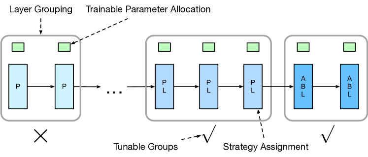
Figure 1: A parameter-efficient fine-tuning design space. It is characterized by (i) layer grouping (how to group consecutive layers), (ii) trainable parameter allocation (how to allocate the number of trainable parameters to layers), (iii) tunable groups (which groups will be finetuned), and (iv) strategy assignment (how to assign proper strategies, such as among Adapter, Prefix, BitFit, and LoRA, to groups).

Instead of designing yet another individual strategy that is equally applied to different pretrained layers, we introduce parameter-efficient fine-tuning design spaces that parameterize both tuning structures and strategies. More concretely, any of these design spaces is characterized by four major components as shown in Figure 1: layer grouping, trainable parameter allocation, tunable groups, and strategy assignment.

Starting from a relatively unconstrained parameter-efficient fine-tuning design space, we progressively refine the space by comparing the overall quality of models randomly sampled from design spaces enforced with different constraints (e.g., each group has the same number of layers). Throughout the experimental process, we discover several design patterns for parameter-efficient fine-tuning, such as group layers in a spindle pattern, allocate the number of trainable parameters to layers uniformly, tune all the groups, and assign proper tuning strategies to different groups. We further introduce new parameter-efficient fine-tuning methods that adopt all these discovered design patterns. Extensive experiments show that our methods consistently outperform investigated parameter-efficient fine-tuning strategies. Although we use T5 (Raffel et al., 2020) and classification tasks as the working example, we find that our methods with all these discovered design patters are applicable to other backbones (e.g., RoBERTa (Liu et al., 2019), BART (Lewis et al., 2020b), and XLNet (Yang et al., 2019)) and different natural language processing tasks (e.g., summarization, machine translation, and eight SuperGLUE datasets).

Our contributions can be summarized as follows: (i) We introduce parameter-efficient fine-tuning design spaces. (ii) Based on these design spaces, we discover several design patterns in parameter-efficient fine-tuning via comprehensive experiments. (iii) Our discovered design patterns lead to parameter-efficient fine-tuning methods, consistently outperforming investigated parameter-efficient fine-tuning strategies across different backbone models and different NLP tasks.

2 Related Work

Our work is closely related to and built upon the research about the network design spaces and parameter-efficient fine-tuning. We discuss the connections and differences below.

Network Design Spaces

A lot of works designed neural network models via an ad-hoc discovery of new design choices that improve performances (Radosavovic et al., 2019), such as the use of deeper architectures or residuals. Recently, there have been works (Radosavovic et al., 2020; You et al., 2020; Radosavovic et al., 2019) performing at the design space level to discover new design principles for convolutional neural networks (Radosavovic et al., 2020) and graph neural networks (You et al., 2020). Inspired by this line of research, we focus on the design space perspective to rethink parameter-efficient fine-tuning, with the goal of discovering design patterns that are applicable to different experimental settings.

Parameter-Efficient Fine-Tuning for NLP

As pretrained models grow in size, storing fine-tuned models becomes exceedingly expensive, and fine-tuning becomes infeasible for those without extremely high compute resources. A growing body of research has been devoted to finding parameter-efficient alternatives for adapting large-scale pretrained models with reduced memory and storage costs. Houlsby et al. (2019b) proposed to adapt large models using bottleneck layers (with skip-connections) between each layer. This idea has been extended in many domains  (Stickland and Murray, 2019; Pfeiffer et al., 2020; Rebuffi et al., 2017; Lin et al., 2020). Other works have aimed to avoid introducing additional parameters by identifying and training only a subset of all model parameters (Zhao et al., 2020; Guo et al., 2020; Mallya et al., 2018; Radiya-Dixit and Wang, 2020; Sung et al., 2021; Zaken et al., 2021). Recent works also explored the idea of rank decomposition based on parameterized hypercomplex multiplications via the Kronecker product (Zhang et al., 2021a) and injecting trainable rank decomposition matrices into each layer (Hu et al., 2021; Karimi Mahabadi et al., 2021). Li and Liang (2021) introduced prefix-tuning that prepends a set of prefixes to autoregressive language models or prepends prefixes for both encoders and decoders. The prefix parameters are updated while the pretrained parameters are fixed. Lester et al. (2021a) proposed a similar method, but only added virtual tokens at the embedding layer of large-scale models rather than discrete prompts (Deng et al., 2022; Zhong et al., 2022). Bari et al. (2022) proposed semi-parametric prompt tuning that converges more easily, where memory prompts are input-adaptive without the need for tuning. Recently, He et al. (2022) and Ding et al. (2022) proposed a unified view of the existing parameter-efficient fine-tuning strategies and illustrated the difference and connections among them. Mao et al. (2022) also introduced a unified framework to combine different methods through mixture-of-experts.

In contrast to these aforementioned works that assign their individual method equally to different pretrained layers, we focus on more general design spaces of parameter-efficient fine-tuning. This could provide a more comprehensive view of parameter-efficient fine-tuning in terms of both the tuning structures and tuning strategies. Through experiments where we progressively refine design spaces, we discover design patterns for parameter-efficient fine-tuning.

3 Components of Design Spaces

When defining design spaces of parameter-efficient fine-tuning, we aim to cover key design components and provide a representative set of choices in each design component. Note that our goal is not to enumerate all possible design spaces, but to demonstrate how the use of design spaces can help inform parameter-efficient fine-tuning research.

Concretely, in our work, the parameter-efficient fine-tuning design spaces are formed by a representative set of choices in parameter-efficient fine-tuning, which consists of the following four components: (i) layer grouping, (ii) trainable parameter allocation, (iii) tunable groups, and (iv) strategy assignment. Following the illustrated design space example in Figure 1, we describe these four design components in detail below and will explore their design choices in Section 4.

Layer Grouping

Different layers in pretrained models capture different information and behave differently. For example, Jawahar et al. (2019) found that the $\{3,4,5,6,7,9,12\}$-th layers have the most representation power in BERT and every layer captures a different type of information ranging from the surface, syntactic, to the semantic level representation of text. For instance, the 9th layer has predictive power for semantic tasks such as checking random swapping of coordinated clausal conjuncts, while the 3rd layer performs best in surface tasks like predicting sentence length. Therefore when adapting these pretrained models to downstream tasks, how to group layers with similar behaviors together is critical to the design and application of proper parameter-efficient fine-tuning strategies. For this design component, we study the patterns of how to group consecutive layers in pretrained models (e.g., transformer layers in T5) during the fine-tuning process.

Trainable Parameter Allocation

In parameter-efficient fine-tuning, the total number of trainable parameters is usually preset, such as a small portion of the total number of parameters in the pretrained models. We will study different design choices for how to allocate a predefined number of trainable parameters to layers.

Tunable Groups

Zaken et al. (2021) found that not all the parameters need to be tuned during fine-tuning on the downstream tasks. For instance, BitFit (Zaken et al., 2021) only updates the bias parameters in pretrained models while freezing the remaining parameters. Thus, we study which groups need to be learned during parameter-efficient fine-tuning to attain better performances.

Strategy Assignment

In order to improve the parameter efficiency, different sets of strategies (Li and Liang, 2021; Lester et al., 2021a; Houlsby et al., 2019a; Hu et al., 2021) have been proposed where only a small number of (extra) parameters are tuned and the remaining parameters in these pretrained models are frozen to adapt their general knowledge to specific down-stream tasks. Inspired by effectiveness of offering architectural flexibility (Zhang et al., 2021a, b), we hypothesize that different groups might benefit from different proper strategies (or combinations) for capturing different types of information. More formally, given a set of individual strategies $\mathcal{A}$ for assignment, for any group $G_{i}$, assign a subset $\mathcal{U}_{i}\subset\mathcal{A}$ to each layer in $G_{i}$.

4 Discovering Design Patterns

Building on these four different design components of PEFT design spaces, we will start from a relatively unconstrained design space and progressively discover the design patterns.

4.1 Design Space Experimental Setup

We first describe our experimental setup for discovering the design patterns. Note that our process is generic for other tasks and future pretrained backbone models.

Datasets

Our process for discovering design patterns of PEFT is based on the average performances on the widely-used GLUE benchmark (Wang et al., 2018). It covers a wide range of natural language understanding tasks. First, single-sentence tasks include (i) Stanford Sentiment Treebank (SST-2) and (ii) Corpus of Linguistic Acceptability (CoLA). Second, similarity and paraphrase tasks include (i) Quora Question Pairs (QQP), (ii) Semantic Textual Similarity Benchmark (STS-B), and (iii) Microsoft Research Paraphrase Corpus (MRPC). Third, inference tasks include (i) Multi-Genre Natural Language Inference (MNLI), (ii) Question Natural Language Inference (QNLI), and (iii) Recognizing Textual Entailment (RTE). To compare performances, the Matthews correlation is measured for CoLA; the Spearman correlation is used for STS-B, and accuracy is measured for the rest GLUE tasks.

Pretrained Backbone Models and Model Settings

We use T5-base/3b (Raffel et al., 2020) as the main pretrained backbone models for discovering design patterns via our PEFT design spaces. We use Hugging Face for our implementations and follow the default settings. During the exploration, we set the total number of trainable parameters (in the percentage of that in the backbone model) to 0.5% by following He et al. (2022).

4.2 Discovering Design Patterns Using T5-base

In this subsection, we describe the empirical process for discovering the design patterns using T5-base (pretrained backbone model) as the working example. Each PEFT design space (denoted as $\mathcal{S}_{i}$) consists of a set of models ($\mathcal{S}_{i}$-models) that satisfy constraints characterizing the space with respect to layer grouping, trainable parameter allocation, tunable groups, and strategy assignment. To discover design patterns, we start from a relatively unconstrained PEFT design space ($\mathcal{S}_{0}$). Then we progressively refine design spaces (from $\mathcal{S}_{0}$ to $\mathcal{S}_{1:4}$) by comparing overall quality of models in design spaces enforced with different constraints (e.g., each group has the same number of layers). To quantify the overall quality of models in any design space $\mathcal{S}_{i}$ with a low-compute, low-epoch regime (Radosavovic et al., 2020), we randomly sample 100 models from $\mathcal{S}_{i}$, fine-tune with 3 epochs, and compute the average of the GLUE average performances.

We emphasize that our goal is to demonstrate how the perspective of design spaces can help inform PEFT research, rather than to find out the “best” design space or method. For computational efficiency, it is beyond the scope of this work to enumerate all possible constraints with respect to the design space components (Section 3).

4.2.1 The Initial $\mathcal{S}_{0}$ Design Space

The initial relatively unconstrained design space $\mathcal{S}_{0}$ consists of all models without constraints on the design space components (Section 3). Individual PEFT strategies consist of Adapter, Prefix, BitFit, and LoRA. One can think of this $\mathcal{S}_{0}$ design space as a set of random models ($\mathcal{S}_{0}$-models) with random design patterns. Specifically, without grouping constraints, each layer of the pretrained layer has a half chance to be tuned: if tuned, random strategies (or combinations) with a random amount of trainable parameters are assigned to that layer.

Before comparing more subtle design patterns such as how to properly assign tunable strategies among Adapter, Prefix, BitFit, and LoRA, we begin with exploring how to group layers and how to allocate the total number of trainable parameters to layers.

4.2.2 The $\mathcal{S}_{1}$ Design Space with Additional Grouping Constraints

Inspired by Radosavovic et al. (2020), we also consider 4 groups ($G_{1},\ldots,G_{4}$, in the order of forward pass) in the experiments . Denote by $N_{i}$ the number of layers in $G_{i}$. As illustrated in Figure 2, we compare the following layer grouping patterns: (i) Increasing ($N_{i+1}>N_{i}$): the number of layers in groups gradually increases; (ii) Uniform ($N_{i+1}=N_{i}$): the number of layers in groups is the same; (iii) Decreasing ($N_{i+1}<N_{i}$): the number of layers in groups gradually decreases; (iv) Spindle (${N_{1}<N_{2}=N_{3}>N_{4}}$): the numbers of layers in groups at both ends are smaller; and (v) Bottleneck ($N_{1}>N_{2}=N_{3}<N_{4}$): the numbers of layers in groups at both ends are bigger.

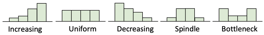
Figure 2: Layer grouping patterns, where the horizontal and vertical axes represent groups ($G_{1},\ldots,G_{4}$) and numbers of layers in groups.

These layer grouping patterns lead to 5 different design spaces. Any of these 5 design spaces consists of all models in the $\mathcal{S}_{0}$ design space that satisfy one of these grouping pattern constraints. To compare the overall model qualities of different design spaces, we (i) randomly sample 100 models from the $\mathcal{S}_{0}$ design space that satisfy each grouping pattern constraint (Figure 2); (ii) fine-tune with 3 epochs; and (iii) compute the average performances for each design space. We will follow this procedure as we progressively add new constraints later.

The averaged performances are shown in Table 1. We find that models from the design space with the spindle grouping pattern (Figure 2) consistently outperform those from the other design spaces across all the 8 GLUE tasks. This may be due to the complexities of information captured in different layers of large pretrained models, which favor information adaptation in the discovered layer grouping pattern.

From now on, we will group layers in a spindle pattern. We refer to $\mathcal{S}_{0}$ with this additional design pattern as the new $\mathcal{S}_{1}$ design space.

Table 1: Average performances (low-compute, low-epoch regime: 100 random models, 3 tuning epochs) on the GLUE datasets using the T5-base pretrained backbone model. We compare adding different layer grouping constraints to the $\mathcal{S}_{0}$ design space.

Layer Grouping	SST-2	MNLI	QNLI	QQP	RTE	STS-B	MRPC	CoLA	Avg
$\mathcal{S}_{0}$-models	76.9	70.1	72.5	73.3	63.6	71.7	73.8	24.3	65.7
Increasing	85.3	74.9	77.2	77.5	66.8	76.2	76.0	33.0	70.8
Uniform	84.8	73.7	78.1	78.6	68.5	77.8	79.2	36.1	72.1
Decreasing	81.9	72.1	78.3	76.7	67.3	75.9	78.6	28.7	70.0
Spindle	86.9	75.5	79.8	79.4	69.8	78.3	80.1	37.3	73.3
Bottleneck	84.5	74.6	76.9	78.1	69.2	76.2	78.6	32.1	71.3

Table 2: Average performances (low-compute, low-epoch regime: 100 random models, 3 tuning epochs) on the GLUE datasets using the T5-base pretrained backbone model. We compare adding different parameter allocation constraints to the $\mathcal{S}_{1}$ design space.

Param Allocation	SST-2	MNLI	QNLI	QQP	RTE	STS-B	MRPC	CoLA	Avg
Increasing	87.2	77.9	79.4	78.7	71.6	77.6	81.4	32.0	73.2
Uniform	87.8	77.4	80.1	80.5	73.9	78.1	80.4	34.3	74.0
Decreasing	86.4	75.8	78.4	77.0	70.4	77.1	78.7	35.8	72.4

4.2.3 The $\mathcal{S}_{2}$ Design Space with Additional Parameter Constraints

We continue to explore design patterns in trainable parameter allocation to refine the $\mathcal{S}_{1}$ design space. Denote by $n_{i}$ the number of trainable parameters for the $i$-th layer of the pretrained backbone model, we compare the following design patterns: (i) Increasing ($n_{i+1}\geq n_{i}$): the number of trainable parameters in every layer gradually increases (or remains the same); (ii) Uniform (${n_{i+1}=n_{i}}$): the number of trainable parameters in every layer is the same; and (iii) Decreasing ($n_{i+1}\leq n_{i}$): the number of trainable parameters in every layer gradually decreases (or remains the same). Following the procedure described in Section 4.2.2, we obtain 100 models for each of these 3 new design spaces. Table 2 reports the average performances of these 3 design spaces. The uniform allocation design pattern obtains the highest GLUE average performance, making this relatively simple, interpretable design pattern favorable.

We will allocate the number of trainable parameters to layers uniformly. We refer to $\mathcal{S}_{1}$ with this additional design pattern as the new $\mathcal{S}_{2}$ design space.

Table 3: Average performances (low-compute, low-epoch regime: 100 random models, 3 tuning epochs) on the GLUE datasets using the T5-base pretrained backbone model. We compare adding different tunable group constraints to the $\mathcal{S}_{2}$ design space.

Tunable Groups	SST-2	MNLI	QNLI	QQP	RTE	STS-B	MRPC	CoLA	Avg
$G_{1}$	82.6	72.1	77.6	70.6	65.3	71.9	77.6	27.6	68.2
$G_{2}$	83.3	72.8	77.5	72.8	63.6	72.8	77.5	27.5	68.4
$G_{3}$	83.6	73.3	78.2	73.3	66.4	71.3	77.9	22.9	68.4
$G_{4}$	83.2	73.0	77.9	73.7	63.9	72.0	77.9	27.9	68.7
$G_{1}$, $G_{2}$	83.5	73.2	78.0	75.4	67.7	73.2	78.0	28.0	69.6
$G_{3}$, $G_{4}$	87.8	74.6	78.3	76.9	68.6	74.3	78.3	28.3	70.7
$G_{1}$, $G_{2}$, $G_{3}$	86.0	75.8	79.0	77.8	71.8	78.8	79.0	33.0	72.6
$G_{2}$, $G_{3}$, $G_{4}$	85.2	76.6	79.1	78.6	70.1	77.6	79.1	31.9	72.2
$\bm{G_{1},G_{2},G_{3},G_{4}}$	88.3	77.4	82.1	81.5	74.9	79.4	81.4	34.3	74.9

4.2.4 The $\mathcal{S}_{3}$ Design Space with Additional Tunable Group Constraints

Before digging into the strategy assignment design patterns, it is necessary to examine which groups need to be tuned. After all, it is only meaningful to study assigning strategies to different groups after we find out which groups need to be fine-tuned. As shown in Table 3, we explore various design patterns in tunable groups to further constrain the $\mathcal{S}_{2}$ design space. Based on the GLUE average performances, we find that all the groups need to be tuned to obtain the best performances. This suggests that all the groups of pretrained layers have captured useful information that should be adapted to the downstream tasks.

We will tune all the groups. We refer to $\mathcal{S}_{2}$ with this additional design pattern as the new $\mathcal{S}_{3}$ design space.

4.2.5 The $\mathcal{S}_{4}$ Design Space with Additional Strategy Constraints

Finally, we study the subtle design pattern with respect to assigning proper strategies by further constraining the derived $\mathcal{S}_{3}$ design space. Specifically, each design space consists of models that assign a subset of {Adapter (A), Prefix (P), BitFit (B), and LoRA (L)} to all layers of any group $G_{i}$ ($i=1,\ldots,4$). We begin by adding different $G_{1}$ strategy assignment constraints to the $\mathcal{S}_{3}$ space. Following the same pattern discovery procedure (Section 4.2.2), we discover strategy assignment patterns for $G_{1}$. Then we progressively add $G_{i}$ ($i>1$) strategy assignment constraints together with the discovered strategy assignment patterns for all $G_{j}$ ($j=1,\ldots,i-1$) to the $\mathcal{S}_{3}$ space. Due to space limit, we present results of this process in the Appendix ($G_{1}$ in Table 8, $G_{2}$ Table 9, $G_{3}$ in Table 10, and $G_{4}$ in Table 11), which suggests strategy assignment of $G_{1}$-(A, L) – $G_{2}$-(A, P) – $G_{3}$-(A, P, B) – $G_{4}$-(P, B, L) for the T5-base pretrained backbone model.

We will assign the discovered proper tuning strategies to groups. We refer to $\mathcal{S}_{3}$ with this additional design pattern as the new $\mathcal{S}_{4}$ design space, which consists of the final $\mathcal{S}_{4}$-model.

4.3 Discovering Design Patterns Using T5-3b

We then repeat the above process on T5-3b to examine if the design patterns we discovered using smaller models (T5-base) still apply when we use larger models. The results are shown in Table 12 (layer grouping), Table 13 (trainable parameter allocation), Table 14 (tunable groups) and Table 15 (strategy assignment) in the Appendix. We observe that the design patterns still apply when larger models like T5-3b are used: (i) grouping layers in a spindle pattern (Table 12), (ii) uniformly allocating the number of trainable parameters to layers (Table 13), (iii) tuning all the groups (Table 14), and (iv) tuning different groups with proper strategies (Table 15). For T5-3b, the discovered proper strategy assignment is $G_{1}$-(P, L) – $G_{2}$-(A, L) – $G_{3}$-(P, B, L) – $G_{4}$-(A, P, B). We refer to the final design space as $\mathcal{S}_{4}$-3b and the final model in this space as $\mathcal{S}_{4}$-3b-model.

Table 4: Performances of different tuning methods on the GLUE datasets using the T5-base (upper part) and T5-3b (lower part) pretrained backbone models, respectively. The results are averaged over 20 random runs (with standard deviations as subscripts). The $\mathcal{S}_{4}$-model and the $\mathcal{S}_{4}$-3b-model perform significantly better than the second-best PEFT methods in all the eight datasets at the significance level $p<0.05(*)$ or even $p<0.01(**)$.

Method	SST-2	MNLI	QNLI	QQP	RTE	STS-B	MRPC	CoLA	Average
full	95.2	87.1	93.7	89.4	80.1	89.4	90.7	51.1	84.5
Adapter	94.6	85.5	89.8	86.7	75.3	86.7	89.1	59.2	83.3
Prefix	94.0	81.6	87.8	83.4	64.3	83.1	84.8	34.0	76.6
BitFit	94.4	84.5	90.6	88.3	74.3	86.6	90.1	57.7	83.3
LoRA	94.8	84.7	91.6	88.5	75.8	86.3	88.7	51.5	82.7
$\mathcal{S}_{4}$-model	$\mathbf{95.5}_{1.7}^{**}$	$\mathbf{87.6}_{1.0}^{**}$	$\mathbf{92.7}_{1.1}^{**}$	$\mathbf{88.8}_{1.0}^{**}$	$\mathbf{80.4}_{2.3}^{*}$	$\mathbf{87.4}_{2.0}^{*}$	$\mathbf{91.2}_{2.4}^{**}$	$\mathbf{62.2}_{3.2}^{*}$	85.7
full	97.4	91.4	96.3	89.7	91.1	90.6	92.5	67.1	89.5
Adapter	96.3	89.9	94.7	87.8	83.4	90	89.7	65.2	87.1
Prefix	96.3	82.8	88.9	85.5	78.3	83.5	85.4	42.7	80.4
BitFit	95.8	89.5	93.5	88.5	86.2	90.7	88.6	64.2	87.1
LoRA	96.2	90.6	94.9	89.1	91.2	91.1	91.1	67.4	88.9
$\mathcal{S}_{4}$-3b-model	$\mathbf{97.2}_{1.8}^{**}$	$\mathbf{91.6}_{1.2}^{**}$	$\mathbf{96.6}_{1.0}^{**}$	$\mathbf{89.5}_{1.5}^{**}$	$\mathbf{91.5}_{2.8}^{*}$	$\mathbf{91.5}_{2.5}^{*}$	$\mathbf{91.9}_{2.0}^{*}$	$\mathbf{69.7}_{3.4}^{*}$	89.9

Table 5: Performances of different tuning methods on GLUE datasets using the RoBERTa-base (upper part) and RoBERTa-large (lower part) pretrained backbone models. The results are averaged over 20 random runs (with standard deviations as subscripts). Here we also include two baselines: (i) $\mathcal{S}_{0}$-model, where all the designs are randomly selected for RoBERTa as in the $\mathcal{S}_{0}$ design space; (ii) $\mathcal{S}_{3}$-model, where strategies are randomly assigned to different RoBERTa layer groups as in the $\mathcal{S}_{3}$ design space. The $\mathcal{S}_{4}$-model and $\mathcal{S}_{4}$-3b-model perform significantly better than the second-best PEFT methods in all the eight datasets at the significance level $p<0.05(*)$ or even $p<0.01(**)$.

Method	SST-2	MNLI	QNLI	QQP	RTE	STS-B	MRPC	CoLA	Average
full	94.8	87.6	92.8	91.9	80.8	90.3	90.2	63.6	86.5
Adapter	94.2	87.1	93.1	90.2	71.5	89.7	88.5	60.8	84.4
Prefix	94.0	86.8	91.3	90.5	74.5	90.3	88.2	61.5	84.6
BitFit	93.7	84.8	91.3	84.5	77.8	90.8	90.0	61.8	84.3
LoRA	94.9	87.5	93.1	90.8	83.1	90.0	89.6	62.6	86.4
$\mathcal{S}_{0}$-model	94.2	95.3	90.4	90.6	75.6	89.6	88.0	60.9	85.6
$\mathcal{S}_{3}$-model	94.3	87.2	92.8	91.0	81.8	90.3	89.2	63.2	86.2
$\mathcal{S}_{4}$-model	$94.8_{1.6}$	$\mathbf{87.8}_{0.8}^{**}$	$\mathbf{93.4}_{1.3}^{**}$	$\mathbf{91.6}_{1.2}^{*}$	$\mathbf{85.8}_{1.8}^{**}$	$90.4_{2.0}^{*}$	$\mathbf{90.0}_{1.8}^{**}$	$\mathbf{63.2}_{3.5}^{*}$	87.1
full	96.4	90.2	94.7	92.2	86.6	92.4	90.9	68.0	88.9
Adapter	96.6	90.5	94.8	91.7	80.1	92.1	90.9	67.8	88.1
Prefix	95.7	87.6	92.1	88.7	82.3	89.6	87.4	62.8	85.7
BitFit	96.1	88.0	93.4	90.2	86.2	90.9	92.7	64.2	87.7
LoRA	96.2	90.6	94.7	91.6	87.4	92.0	89.7	68.2	88.8
$\mathcal{S}_{0}$-model	95.5	86.5	92.3	89.8	84.6	89.2	86.3	61.2	85.6
$\mathcal{S}_{3}$-model	96.3	89.4	93.8	90.2	85.9	90.8	90.9	63.4	87.6
$\mathcal{S}_{4}$-3b-model	$\mathbf{96.6}_{1.3}^{**}$	$\mathbf{90.8}_{1.1}^{*}$	$\mathbf{95.1}_{0.8}^{**}$	$\mathbf{92.0}_{1.2}^{**}$	$87.2_{2.8}$	$\mathbf{92.3}_{2.2}^{*}$	$91.8_{1.8}^{**}$	$\mathbf{68.4}_{3.2}^{*}$	89.3

5 Evaluation

The $\mathcal{S}_{4}$-model (Section 4.2.5) and $\mathcal{S}_{4}$-3b-model (Section 4.3) adopt all the design patterns that have been discovered by using T5-base and T5-3b, respectively. As a result, they are both new methods of PEFT. We will evaluate their effectiveness when applied to different pretrained backbone models and different NLP tasks.

5.1 Experimental Setup

Datasets

Besides the GLUE datasets (Wang et al., 2018) (Section 4.1), we further evaluate our methods on two generation tasks used by He et al. (2022): (i) Abstractive Summarization using XSum (Narayan et al., 2018), and (ii) Machine Translation using the WMT 2016 en-ro dataset (Bojar et al., 2016). We report ROUGE scores (Lin, 2004) on the XSum test set, and BLEU scores (Papineni et al., 2002) on the en-ro test set.

Models and Model Settings

We mainly compare our methods with the following baselines: (i) Full Fine-tuning (full): it fine-tunes all the model parameters in the pretrained models; (ii) Adapter (Houlsby et al., 2019a): it adds adapter modules to each transformer layer; (iii) Prefix (Li and Liang, 2021): it optimizes a set of small continuous vectors prepended to transformer layers; (iv) BitFit (Zaken et al., 2021): it only updates the bias terms in pretrained models; (v) LoRA (Hu et al., 2021): it decomposes the attention weight into low-rank matrices to reduce the number of trainable parameters. Besides T5 (Raffel et al., 2020), we additionally apply our methods to other backbone models including RoBERTa-base/large (Liu et al., 2019) and BART-base/large (Lewis et al., 2020a). We use the default settings. We set the total number of trainable parameters (in the percentage of that in the backbone model) by following He et al. (2022). Specifically, this value is set to 0.5% for Adapter, Prefix, LoRA, and our methods, and 0.1% for BitFit.

For all the experiments, we followed Liu et al. (2019) to set the linear decay scheduler with a warmup ratio of 0.06 for training. The batch size was 128 for base models and 64 for large models. The maximum learning rate was $5e-5$ and the maximum number of training epochs was set to be either $5$ or $10$. All the experiments were performed using 8 A100 GPUs.

Table 6: Performances of different tuning methods on generation tasks (XSUM and en-ro) using the BART-base (upper part) and BART-large (lower part) pretrained backbone models.

Method	XSUM(R-1/2/L)	en-ro (BLEU)
full	40.5/19.2/34.8	34.5
Adapter	37.7/17.9/33.1	33.3
Prefix	38.2/18.4/32.4	33.8
BitFit	37.2/17.5/31.4	33.2
LoRA	38.9/18.6/33.5	33.6
PA	39.3/18.7/33.8	33.8
$\mathcal{S}_{4}$-model	40.2/19.3/34.2	34.1
full	45.1/22.3/37.2	37.9
Adapter	43.8/20.8/35.7	35.3
Prefix	43.4/20.4/35.5	35.6
BitFit	42.8/18.7/33.2	35.2
LoRA	42.9/19.4/34.8	35.8
PA	43.9/20.6/35.6	36.4
$\mathcal{S}_{4}$-3b-model	44.3/21.7/36.8	37.2

5.2 Effectiveness on GLUE with T5 Backbones

With our discovered design patterns, we fine-tune T5-base ($\mathcal{S}_{4}$-model) and T5-3b ($\mathcal{S}_{4}$-3b-model) on GLUE and compare them with all the baseline methods. The results are shown in Table 4, where the key measure is the GLUE average performance (last column). We find that our $\mathcal{S}_{4}$-model and $\mathcal{S}_{4}$-3b-model consistently outperform the investigated methods in the key measure. By tuning only $0.5\%$ parameters, our methods even outperform the full fine-tuning baseline where all the parameters are tuned, indicating the effectiveness of our discovered PEFT design patterns.

5.3 General Effectiveness on GLUE with RoBERTa Backbones

We directly apply the $\mathcal{S}_{4}$-model and $\mathcal{S}_{4}$-3b-model (adopting design patterns discovered using T5-base and T5-3b) to fine-tune the RoBERTa-base and RoBERTa-large pretrained backbone models (with no extra discovery process), respectively. We keep all the other settings the same and evaluate them on GLUE datasets. We also compare with variant methods randomly sampled from two design spaces: (i) $\mathcal{S}_{0}$-model, where all the designs are randomly selected for RoBERTa as in $\mathcal{S}_{0}$; (ii) $\mathcal{S}_{3}$-model, where strategies are randomly assigned to different RoBERTa layer groups as in $\mathcal{S}_{3}$. Table 5 shows that (i) the design patterns (adopted by $\mathcal{S}_{4}$-model and $\mathcal{S}_{4}$-3b-model) discovered using T5 models are applicable to the RoBERTa backbone models and outperform the investigated methods in GLUE average performances with no extra discovery process;(ii) improved performances from $\mathcal{S}_{0}$-models, $\mathcal{S}_{3}$-models, to $\mathcal{S}_{4}$-(3b)-models support adding more constraints in the pattern discovery process (Section 4).

5.4 General Effectiveness on Generation Tasks with BART Backbones

Like in Section 5.3, we further directly apply the $\mathcal{S}_{4}$-model and $\mathcal{S}_{4}$-3b-model (adopting design patterns discovered using T5-base and T5-3b) to fine-tune the BART-base and BART-large pretrained backbone models (without additional discovery process.), respectively. We evaluate the models on two generation tasks: summarization (XSUM) and machine translation (en-ro) following He et al. (2022). We also compare with PA (parallel adapter) using the same number of trainable parameters (He et al., 2022). Table 6 shows that our methods, although adopting design patterns discovered from classification tasks using T5, still outperform investigated PEFT strategies on generation tasks with different BART backbones.

6 Conclusion

PEFT adapts knowledge in pretrained models to down-stream tasks in a more parameter-efficient fashion. Instead of focusing on designing another strategy in the first place, we introduced PEFT design spaces. We empirically discovered several design patterns in PEFT. These design patterns led to new PEFT methods. Experiments showed that these methods consistently outperform investigated PEFT strategies across different backbone models and different tasks in natural language processing.

Appendix A More Experimental Results

Table 7: Average performances (low-compute, low-epoch regime: 100 random models, tuning epochs $=1,2,3,4,20$ for five different blocks) on the GLUE datasets using the T5-base pretrained backbone model. We compare adding different grouping constraints to the $\mathcal{S}_{0}$ design space.

Grouping Patterns	SST-2	MNLI	QNLI	QQP	RTE	STS-B	MRPC	CoLA	Avg
1 epochs
Increasing	73.2	63.3	67.8	68.8	63.8	67.2	64.1	11.0	59.9
Uniform	72.8	64.1	63.4	63.4	62.5	69.8	65.8	12.1	59.2
Decreasing	72.4	63.2	65.1	69.8	59.3	62.7	63.6	18.7	59.4
Spindle	72.6	64.8	66.8	71.1	62.1	62.3	64.8	12.3	59.6
Bottleneck	72.2	63.7	65.3	68.3	61.2	63.2	66.6	12.1	59.0
2 epochs
Increasing	76.2	69.3	73.2	76.5	65.8	72.2	74.0	21.0	66.0
Uniform	74.8	70.9	74.1	75.6	66.5	73.4	71.2	22.1	66.1
Decreasing	71.4	70.1	72.1	76.8	64.3	71.7	73.6	18.7	64.8
Spindle	76.6	71.9	71.8	74.4	67.5	73.5	71.8	22.3	66.2
Bottleneck	74.2	71.1	69.6	73.3	65.2	73.3	73.6	24.1	65.5
3 epochs
Increasing	85.3	74.9	77.2	77.5	66.8	76.2	76.0	33.0	70.8
Uniform	84.8	73.7	78.1	78.6	68.5	77.8	79.2	36.1	72.1
Decreasing	81.9	72.1	78.3	76.7	67.3	75.9	78.6	28.7	69.9
Spindle	86.9	75.5	79.8	79.4	69.8	78.3	80.1	47.3	74.6
Bottleneck	84.5	74.6	76.9	78.1	69.2	76.2	78.6	32.1	71.3
4 epochs
Increasing	88.3	78.5	80.2	80.5	70.8	80.2	80.0	37.0	74.4
Uniform	88.8	78.9	81.9	81.5	71.5	80.8	81.4	39.1	75.4
Decreasing	87.6	74.1	80.8	81.7	79.3	78.9	79.6	38.7	75.1
Spindle	89.6	79.8	83.6	82.8	71.8	81.3	82.1	39.3	76.3
Bottleneck	86.5	77.6	82.7	81.1	70.2	70.9	81.6	36.1	73.3
20 epochs
Increasing	92.3	83.3	86.2	82.5	71.8	82.2	84.0	51.0	79.1
Uniform	92.8	83.9	86.1	83.6	72.5	83.8	84.2	52.1	79.9
Decreasing	91.4	82.1	85.1	83.1	69.3	81.7	83.6	48.7	78.1
Spindle	93.6	84.8	87.8	84.4	73.5	84.3	85.8	52.3	80.8
Bottleneck	92.1	82.6	85.6	83.3	71.2	83.2	84.6	52.1	79.3

Table 8: Average performances (low-compute, low-epoch regime: 100 random models, 3 tuning epochs) on the GLUE datasets using the T5-base pretrained backbone model. We compare adding different $G_{1}$ strategy assignment constraints to the $\mathcal{S}_{3}$ design space.

Strategy Assignment	SST-2	MNLI	QNLI	QQP	RTE	STS-B	MRPC	CoLA	Avg
$G_{1}$-Adapter (A)	89.8	83.5	84.9	80.8	72.5	80.8	78.5	37.7	76.1
$G_{1}$-Prefix (P)	89.3	83.1	84.4	80.1	70.1	80.0	77.6	33.0	74.7
$G_{1}$-BitFit (B)	89.0	82.9	84.1	81.4	72.0	81.1	77.0	30.8	74.8
$G_{1}$-LoRA (L)	89.9	83.6	85.0	81.1	71.8	81.0	78.8	35.3	75.8
$G_{1}$-(P, L)	89.1	82.8	85.1	81.2	71.9	81.5	79.1	35.0	75.7
$G_{1}$-(A, P)	89.8	82.8	84.8	81.1	72.2	81.3	79.2	36.4	75.9
$G_{1}$-(A, L)	89.6	83.8	85.6	81.3	72.9	81.7	79.5	36.8	76.4
$G_{1}$-(A, P, L)	89.6	83.5	85.2	81.5	72.2	81.4	79.2	35.2	75.9
$G_{1}$-(P, B, L)	89.3	83.6	85.5	81.6	72.3	81.0	78.8	35.7	76.0
$G_{1}$-(A, P, B)	89.2	83.3	84.8	81.8	72.5	81.1	78.6	35.6	75.8
$G_{1}$-(A, B, L)	89.8	83.4	84.8	81.1	72.6	81.6	79.4	34.8	75.9
$G_{1}$-(A, P, B, L)	90.0	83.1	85.3	81.6	72.6	81.4	79.2	36.5	76.1

Table 9: Average performances (low-compute, low-epoch regime: 100 random models, 3 tuning epochs) on the GLUE datasets using the T5-base pretrained backbone model. We compare adding different $G_{2}$ strategy assignment constraints with $G_{1}$-(L, A) to the $\mathcal{S}_{3}$ design space.

Strategy Assignment	SST-2	MNLI	QNLI	QQP	RTE	STS-B	MRPC	CoLA	Avg
$G_{2}$-Adapter (A)	91.6	84.3	85.5	82.3	73.5	82.8	81.3	38.8	77.5
$G_{2}$-Prefix (P)	89.6	84.0	86.5	81.5	73.3	82.5	80.5	36.2	76.7
$G_{2}$-BitFit (B)	91.2	83.6	85.7	82.9	72.6	82.6	80.8	33.1	76.5
$G_{2}$-LoRA (L)	91.4	84.4	86.1	82.0	72.8	81.8	81.6	39.8	77.4
$G_{2}$-(P, L)	91.6	84.6	86.8	81.8	73.8	82.8	82.0	38.5	77.7
$G_{2}$-(A, P)	92.2	84.2	87.1	82.2	74.4	83.0	82.5	40.8	78.3
$G_{2}$-(A, L)	92.0	84.4	86.5	81.8	73.6	82.6	82.2	40.1	77.9
$G_{2}$-(A, P, L)	91.8	84.8	86.8	81.8	74.1	83.0	82.1	37.9	77.7
$G_{2}$-(P, B, L)	91.6	84.1	87.1	82.0	74.0	82.9	82.4	35.8	77.4
$G_{2}$-(A, P, B)	91.8	84.2	86.8	82.1	73.7	83.3	82.2	41.2	78.1
$G_{2}$-(A, B, L)	92.2	84.3	86.1	82.0	74.1	83.2	82.0	37.6	77.6
$G_{2}$-(A, P, B, L)	92.0	84.1	87.0	81.9	74.2	83.1	81.3	42.4	78.1

Table 10: Average performances (low-compute, low-epoch regime: 100 random models, 3 tuning epochs) on the GLUE datasets using the T5-base pretrained backbone model. We compare adding different $G_{3}$ strategy assignment constraints with $G_{1}$-(L, A) – $G_{2}$-(P, A) to the $\mathcal{S}_{3}$ design space.

Strategy Assignment	SST-2	MNLI	QNLI	QQP	RTE	STS-B	MRPC	CoLA	Avg
$G_{3}$-Adapter (A)	92.5	85.3	87.5	83.3	73.9	84.0	83.8	44.9	79.4
$G_{3}$-Prefix (P)	91.5	84.7	86.7	82.6	74.2	83.8	82.9	40.5	78.4
$G_{3}$-BitFit (B)	91.9	84.3	87.0	82.0	73.6	84.1	83.3	36.1	77.8
$G_{3}$-LoRA (L)	92.8	85.4	87.8	83.5	74.7	82.4	84.0	44.0	79.3
$G_{3}$-(P, L)	93.0	85.2	88.3	83.8	75.2	84.4	84.2	37.9	79.0
$G_{3}$-(A, P)	92.4	85.6	88.1	83.6	75.0	84.2	84.0	41.8	79.3
$G_{3}$-(A, L)	92.0	85.9	88.2	83.1	75.3	84.3	83.9	42.2	79.4
$G_{3}$-(A, P, L)	92.6	86.0	87.5	83.4	75.6	84.6	83.5	43.9	79.6
$G_{3}$-(P, B, L)	92.7	85.8	87.2	83.7	75.2	84.5	83.8	40.8	79.2
$G_{3}$-(A, P, B)	93.3	85.8	88.6	84.0	75.5	84.9	84.1	42.1	79.8
$G_{3}$-(A, B, L)	93.7	86.5	88.0	83.2	75.8	84.2	84.2	39.7	79.4
$G_{3}$-(A, P, B, L)	93.3	85.6	87.7	83.8	75.2	84.3	84.4	41.6	79.4

Table 11: Average performances (low-compute, low-epoch regime: 100 random models, 3 tuning epochs) on the GLUE datasets using the T5-base pretrained backbone model. We compare adding different $G_{4}$ strategy assignment constraints with $G_{1}$-(A, L) – $G_{2}$-(A, P) – $G_{3}$-(A, P, B) to the $\mathcal{S}_{3}$ design space.

Strategy Assignment	SST-2	MNLI	QNLI	QQP	RTE	STS-B	MRPC	CoLA	Avg
$G_{4}$-Adapter (A)	93.8	85.8	88.6	84.8	76.3	85.8	86.0	48.5	81.2
$G_{4}$-Prefix (P)	93.5	85.2	88.3	83.6	76.8	85.3	85.6	44.8	80.3
$G_{4}$-BitFit (B)	94.1	85.3	88.9	84.4	77.1	85.4	86.2	46.1	80.9
$G_{4}$-LoRA (L)	94.0	86.0	89.2	85.0	77.2	85.5	85.8	47.7	81.3
$G_{4}$-(P, L)	94.3	86.2	89.3	85.8	78.0	86.0	88.2	47.2	81.8
$G_{4}$-(A, P)	94.1	86.2	89.6	85.4	77.9	86.2	86.9	45.3	81.4
$G_{4}$-(A, L)	94.2	85.9	89.2	85.5	77.8	86.2	88.0	46.8	81.7
$G_{4}$-(A, P, L)	94.1	85.8	88.8	85.7	77.4	86.5	87.9	44.8	81.3
$G_{4}$-(P, B, L)	94.6	86.4	90.4	86.1	78.2	86.8	88.5	47.2	82.3
$G_{4}$-(A, P, B)	94.5	86.0	89.6	86.0	78.0	86.2	88.1	44.8	81.6
$G_{4}$-(A, B, L)	94.3	86.4	89.2	85.6	78.2	86.4	88.3	46.6	81.9
$G_{4}$-(A, P, B, L)	94.2	86.2	89.2	85.9	78.5	86.1	88.0	45.3	81.6

Table 12: Average performances (low-compute, low-epoch regime: 100 random models, 3 tuning epochs) on the GLUE datasets using the T5-3b pretrained backbone model. We compare adding different layer grouping constraints to the $\mathcal{S}_{0}$ design space.

Grouping Patterns	SST-2	MNLI	QNLI	QQP	RTE	STS-B	MRPC	CoLA	Avg
$\mathcal{S}_{0}$-models	80.3	72.1	74.7	72.8	76.9	75.2	71.0	32.2	69.4
Increasing	84.4	75.7	83.0	78.3	82.7	80.3	76.3	42.1	75.3
Uniform	86.8	77.1	82.6	76.2	83.8	81.6	77.3	48.9	76.8
Decreasing	83.2	74.3	81.8	77.3	82.8	79.9	76.5	40.8	74.5
Spindle	88.6	78.8	83.7	77.7	84.2	80.9	78.3	44.6	77.1
Bottleneck	86.3	77.0	82.2	75.6	83.3	80.2	77.1	41.5	75.4

Table 13: Average performances (low-compute, low-epoch regime: 100 random models, 3 tuning epochs) on the GLUE datasets using the T5-3b pretrained backbone model. We compare adding different layer parameter constraints to the $\mathcal{S}_{1}$ design space.

Parameter Allocation	SST-2	MNLI	QNLI	QQP	RTE	STS-B	MRPC	CoLA	Avg
Increasing	90.3	79.3	84.9	79.3	85.2	82.8	79.2	50.1	78.9
Uniform	90.6	80.8	84.6	79.7	85.5	82.4	78.9	50.8	79.1
Decreasing	88.6	78.2	83.5	78.1	84.4	81.5	78.1	49.6	77.7

Table 14: Average performances (low-compute, low-epoch regime: 100 random models, 3 tuning epochs) on the GLUE datasets using the T5-3b pretrained backbone model. We compare adding different tuning groups constraints to the $\mathcal{S}_{2}$ design space.

Tunable Groups	SST-2	MNLI	QNLI	QQP	RTE	STS-B	MRPC	CoLA	Avg
$G_{1}$	88.3	78.3	82.2	77.4	82.1	80.7	76.1	49.4	76.8
$G_{2}$	89.1	78.8	82.1	77.2	82.3	81.2	76.4	49.6	77.1
$G_{3}$	89.6	78.5	82.6	78.1	83.8	81.9	77.4	48.7	77.5
$G_{4}$	89.8	79.3	82.7	77.9	83.5	81.9	77.9	48.5	77.1
$G_{1}$, $G_{2}$	90.1	80.2	83.4	78.5	84.3	82.4	78.5	51.1	78.5
$G_{3}$, $G_{4}$	90.5	80.6	83.8	78.7	84.2	83	78.2	50.3	78.6
$G_{1}$, $G_{2}$, $G_{3}$	90.6	80.3	84.9	79.3	84.7	82.9	79.3	50.2	79.0
$G_{2}$, $G_{3}$, $G_{4}$	90.8	80.9	84.6	79.1	85.1	83.1	79.1	49.2	78.9
$\bm{G_{1}}$, $\bm{G_{2}}$, $\bm{G_{3}}$, $\bm{G_{4}}$	91.1	81.4	85.2	80.4	85.9	83.5	80.0	51.6	79.9

Table 15: Average performances (low-compute, low-epoch regime: 100 random models, 3 tuning epochs) on the GLUE datasets using the T5-3b pretrained backbone model. We compare adding different strategy assignment constraints following the process in Section 4.2.5.

Strategy Assignment	SST-2	MNLI	QNLI	QQP	RTE	STS-B	MRPC	CoLA	Avg
$G_{1}$-Adapter (A)	91.1	81.4	86.1	80.5	86.7	83.3	80.1	50.8	80.0
$G_{1}$-Prefix (P)	90.8	81.1	85.5	80.2	86.2	83.1	79.8	50.2	79.6
$G_{1}$-BitFit (B)	90.2	81.3	85.1	79.6	85.8	82.8	79.6	49.5	79.2
$G_{1}$-LoRA (L)	91.4	81.9	86.2	80.8	86.4	83.9	80.8	49.6	80.0
$G_{1}$-(P, L)	91.8	82.9	86.8	81.3	87.1	84.2	81.6	52.3	81.0
$G_{1}$-(A, P)	91.3	81.9	86.4	81.1	85.6	83.7	80.7	52.8	80.1
$G_{1}$-(A, L)	91.6	82.3	86.1	81.5	85.8	84.9	81.5	51.8	80.6
$G_{1}$-(A, P, L)	91.1	81.7	85.8	81.2	86.4	84.2	80.9	52.3	80.4
$G_{1}$-(P, B, L)	91.5	82.8	86.3	81.4	86.1	83.6	81.2	51.5	80.5
$G_{1}$-(A, P, B)	91.3	82.3	86.7	80.8	86.8	84.3	80.7	51.8	80.5
$G_{1}$-(A, B, L)	91.7	82.5	86.2	81.3	86.3	84.6	81.3	51.7	80.7
$G_{1}$-(A, P, B, L)	91.6	82.3	86.2	81.1	86.6	84.2	81.1	51.1	80.5
$G_{2}$-Adapter (A)	92.1	82.5	86.4	81.8	87.2	84.8	81.8	53.8	81.3
$G_{2}$-Prefix (P)	91.8	83.1	87.2	81.6	86.2	84.4	81.1	52.8	81.0
$G_{2}$-BitFit (B)	91.2	82.1	86.4	81.1	86.3	84.6	80.3	53.1	80.6
$G_{2}$-LoRA (L)	92.6	82.9	87.5	81.3	87.4	85.1	81.9	52.2	81.4
$G_{2}$-(P, L)	91.6	82.7	87.6	81.6	87.8	85.3	82.1	52.8	81.4
$G_{2}$-(A, P)	92.1	83.3	87.5	81.9	87.4	85.5	81.8	53.1	81.5
$G_{2}$-(A, L)	92.5	83.7	88.1	82.2	87.4	85.7	82.9	53.6	82.1
$G_{2}$-(A, P, L)	92.3	83.4	87.4	81.6	87.1	85.3	81.4	53.2	81.4
$G_{2}$-(P, B, L)	91.8	83.1	87.4	81.5	87.2	85.1	82.7	53.8	81.5
$G_{2}$-(A, P, B)	91.5	82.6	87.8	81.3	86.5	85.2	82.1	54.2	81.4
$G_{2}$-(A, B, L)	92.6	83.5	87.2	82	87.3	86.5	82.5	52.8	81.8
$G_{2}$-(A, P, B, L)	92.8	83.2	87.6	81.6	87.5	85.5	82.4	51.2	81.5
$G_{3}$-Adapter (A)	92.6	84.1	88.3	81.8	87.8	85.4	82.8	55.2	82.2
$G_{3}$-Prefix (P)	92.1	83.3	87.6	81.4	87.1	85.4	82.6	53.5	81.6
$G_{3}$-BitFit (B)	92.4	83.9	88.4	82.1	87.2	85.8	82.4	53.3	81.9
$G_{3}$-LoRA (L)	93.1	84.3	87.7	82.4	87.8	86.2	83.1	54.3	82.3
$G_{3}$-(P, L)	92.8	84.1	88.7	82.6	88.2	86.2	83.3	54.7	82.6
$G_{3}$-(A, P)	93.1	83.8	89.1	82.3	88.1	85.8	82.6	55.1	82.5
$G_{3}$-(A, L)	92.7	84.5	88.4	82.8	88.2	86.1	83.5	54.6	82.6
$G_{3}$-(A, P, L)	92.8	84.6	88.1	82.5	87.7	85.5	83.2	53.8	82.3
$G_{3}$-(P, B, L)	93.6	84.9	89.3	83.1	88.2	86.5	83.9	55.8	83.2
$G_{3}$-(A, P, B)	93.3	83.9	88.5	82.2	88.4	86.2	83.5	55.3	82.6
$G_{3}$-(A, B, L)	93.4	84.2	88.9	82.6	87.8	85.8	84.2	54.9	82.7
$G_{3}$-(A, P, B, L)	92.2	84.4	88.7	82.3	88.5	86.2	84.2	54.2	82.5
$G_{4}$-Adapter (A)	92.8	85.2	89.1	83.5	87.8	86.5	84.2	56.3	83.2
$G_{4}$-Prefix (P)	92.8	84.6	89.5	82.6	87.4	86.5	83.8	55.8	82.8
$G_{4}$-BitFit (B)	93.8	84.9	89.5	83.3	88.7	86.8	84.4	55.2	83.3
$G_{4}$-LoRA (L)	93.3	84.7	89.3	82.7	88.3	86.2	82.7	54.7	82.7
$G_{4}$-(P, L)	93.8	85.3	89.6	83.6	88.6	86.8	84.6	56.3	83.5
$G_{4}$-(A, P)	93.8	84.9	89.8	84.3	88.5	86.6	84.8	56.7	83.6
$G_{4}$-(A, L)	93.7	85.6	89.5	84.1	88.2	86.6	85.2	55.4	83.5
$G_{4}$-(A, P, L)	94.2	85.2	89.6	83.9	88.2	86.4	84.9	55.9	83.5
$G_{4}$-(P, B, L)	93.8	85.9	89.8	83.6	88.6	86.9	85.2	56.3	83.7
$G_{4}$-(A, P, B)	94.4	85.7	90.1	84.8	88.9	87.2	85.3	57.3	84.2
$G_{4}$-(A, B, L)	93.8	85.3	89.5	84.1	88.8	86.7	85.5	56.6	83.7
$G_{4}$-(A, P, B, L)	94.1	85.4	89.7	84.4	88.5	86.5	85.2	56.8	83.8

Table 16: Average performances (low-compute, low-epoch regime: 100 random models, 3 tuning epochs) on the GLUE datasets using the T5-base pretrained backbone model. We compare adding different layer grouping constraints to the $\mathcal{S}_{0}$ design space. Layer grouping is based on 8 groups.

Layer Grouping	SST-2	MNLI	QNLI	QQP	RTE	STS-B	MRPC	CoLA	Avg
$\mathcal{S}_{0}$-models	76.9	70.1	72.5	73.3	63.6	71.7	73.8	24.3	65.7
Increasing	$83.2$	$74.1$	$76.6$	$77.1$	$67.7$	76.8	74.7	30.0	70.0
Uniform	83.6	73.4	78.0	77.9	68.2	76.4	78.6	34.2	71.3
Decreasing	80.3	71.6	77.4	75.5	67.0	75.3	77.2	26.4	68.9
Spindle	86.2	74.3	79.1	78.6	68.5	77.4	79.5	35.1	72.3
Bottleneck	83.2	73.1	75.8	77.6	67.9	75.3	78.2	31.4	70.3

Appendix B General Effectiveness on SuperGLUE with XLNet Backbones

We also directly use the $\mathcal{S}_{4}$-model and $\mathcal{S}_{4}$-3b-model (adopting design patterns discovered using T5-base and T5-3b) to fine-tune the XLNet-base and XLNet-large pretrained backbone models without any extra discovery process. We keep all the other settings the same and evaluate them on SuperGLUE datasets. Table 17 reiterates the fact that our PEFT design patterns discovered from T5 models are generelizable to the XLNet backbone models and outperform the investigated methods in other tasks (SuperGLUE) with no additional discovery process.

Table 17: Performances of different tuning methods on the SuperGLUE datasets using the XLNet-base (upper part) and XLNet-large (lower part) pretrained backbone models, respectively. The results are averaged over 10 random runs. The $\mathcal{S}_{4}$-model and $\mathcal{S}_{4}$-3b-model perform significantly better than the second-best PEFT methods in all the eight datasets at the significance level $p<0.05$ (*) or even $p<0.01$ (**).

Method	BoolQ	CB	COPA	MultiRC	ReCoRD	RTE	WiC	WSC	Average
Adapter	72.8	71.3/78.0	64.0	67.0/24.5	71.0/71.8	76.2	65.0	60.8	66.2
Prefix	72.0	70.5/77.0	63.3	66.4/23.8	69.9/71.0	75.5	64.4	60.8	65.9
BitFit	71.8	70.0/76.2	62.8	65.8/22.6	69.4/70.6	74.5	64.8	60.6	65.2
LoRA	72.2	71.1/77.8	64.7	67.4/24.8	70.8/71.3	76.8	65.1	61.1	66.4
$\mathcal{S}_{4}$-model	$\mathbf{73.8}^{**}$	$\mathbf{71.7/78.4}^{*}$	$\mathbf{65.9}^{**}$	$\mathbf{68.2/25.5}^{**}$	$\mathbf{71.1/72.0}^{*}$	$\mathbf{78.4}^{**}$	$\mathbf{65.8}^{*}$	$\mathbf{62.6}^{*}$	67.5
Adapter	74.4	71.4/81.1	67.4	68.8/26.4	71.7/72.4	80.8	68.0	64.6	68.8
Prefix	72.4	70.0/78.3	66.9	68.8/25.8	70.9/71.2	78.8	66.9	64.0	67.7
BitFit	71.1	70.7/79.8	68.0	68.6/25.4	71.1/71.6	80.4	67.2	64.3	68.1
LoRA	74.1	72.1/80.9	67.9	69.1/26.8	72.0/72.8	81.0	67.8	64.4	69.0
$\mathcal{S}_{4}$-3b-model	$\mathbf{76.8}^{**}$	$\mathbf{74.6/81.9}^{**}$	$\mathbf{68.6}^{**}$	$\mathbf{69.5/27.1}^{*}$	$\mathbf{72.4/73.3}^{*}$	$\mathbf{81.2}^{*}$	$\mathbf{68.2}^{**}$	$\mathbf{64.8}^{*}$	69.7

Table 18: Total training time (low-compute, low-epoch regime: 100 random models, 3 tuning epochs) on the GLUE datasets using the T5-base pretrained backbone model with 8 A100 GPUs from $\mathcal{S}_{0}$ to $\mathcal{S}_{1}$.

SST-2	MNLI	QNLI	QQP	RTE	STS-B	MRPC	CoLA
18 mins	22 mins	20 mins	40 mins	8 mins	12 mins	8 mins	6 mins

Appendix C On the Discovery Sequence

In this work, we follow the discovery sequence of “grouping patterns – trainable parameter allocation – tunable groups – strategy assignment”:

1. To explore and understand the design patterns in all the layers in large pre-trained models in scale, it is necessary and more efficient to study the layers in the unit of groups. So we start with the grouping patterns.

2. Once figuring out the optimal grouping patterns, it is then important to explore how to allocate the trainable parameters to these different groups in order to study more subtle designs with fair comparisons (e.g., this would allow comparing different patterns of strategy assignments without the impact from different trainable parameters.).

3. Next, it becomes influential to examine which groups need to be learned during fine-tuning before we dig into the strategy assignment patterns. Because it is only meaningful to study assigning strategies to different groups after we figure out which groups need to be learned.

4. Finally, we study the tuning strategy assignment, which is the most subtle design.

References

- Devlin et al. (2019) Jacob Devlin, Ming-Wei Chang, Kenton Lee, and Kristina Toutanova. Bert: Pre-training of deep bidirectional transformers for language understanding. In NAACL-HLT, 2019.
- Liu et al. (2019) Yinhan Liu, Myle Ott, Naman Goyal, Jingfei Du, Mandar Joshi, Danqi Chen, Omer Levy, Mike Lewis, Luke Zettlemoyer, and Veselin Stoyanov. Roberta: A robustly optimized bert pretraining approach. arXiv preprint arXiv:1907.11692, 2019.
- Yang et al. (2019) Zhilin Yang, Zihang Dai, Yiming Yang, Jaime Carbonell, Russ R Salakhutdinov, and Quoc V Le. Xlnet: Generalized autoregressive pretraining for language understanding. In Advances in neural information processing systems, pages 5754–5764, 2019.
- Joshi et al. (2019) Mandar Joshi, Danqi Chen, Yinhan Liu, Daniel S. Weld, Luke Zettlemoyer, and Omer Levy. Spanbert: Improving pre-training by representing and predicting spans. Transactions of the Association for Computational Linguistics, 8:64–77, 2019.
- Sun et al. (2019) Yu Sun, Shuohuan Wang, Yukun Li, Shikun Feng, Xuyi Chen, Han Zhang, Xin Tian, Danxiang Zhu, Hao Tian, and Hua Wu. Ernie: Enhanced representation through knowledge integration. arXiv preprint arXiv:1904.09223, 2019.
- Clark et al. (2019) Kevin Clark, Minh-Thang Luong, Quoc V Le, and Christopher D Manning. Electra: Pre-training text encoders as discriminators rather than generators. In International Conference on Learning Representations, 2019.
- Lewis et al. (2020a) Mike Lewis, Yinhan Liu, Naman Goyal, Marjan Ghazvininejad, Abdelrahman Mohamed, Omer Levy, Ves Stoyanov, and Luke Zettlemoyer. Bart: Denoising sequence-to-sequence pre-training for natural language generation, translation, and comprehension. SCL, 2020a.
- Bao et al. (2020) Hangbo Bao, Li Dong, Furu Wei, Wenhui Wang, Nan Yang, Xiaodong Liu, Yu Wang, Songhao Piao, Jianfeng Gao, Ming Zhou, et al. Unilmv2: Pseudo-masked language models for unified language model pre-training. arXiv preprint arXiv:2002.12804, 2020.
- He et al. (2020) Pengcheng He, Xiaodong Liu, Jianfeng Gao, and Weizhu Chen. Deberta: Decoding-enhanced bert with disentangled attention. arXiv preprint arXiv:2006.03654, 2020.
- Raffel et al. (2020) Colin Raffel, Noam Shazeer, Adam Roberts, Katherine Lee, Sharan Narang, Michael Matena, Yanqi Zhou, Wei Li, and Peter J. Liu. Exploring the limits of transfer learning with a unified text-to-text transformer, 2020.
- Ziems et al. (2022) Caleb Ziems, Jiaao Chen, Camille Harris, Jessica Anderson, and Diyi Yang. VALUE: Understanding dialect disparity in NLU. In Proceedings of the 60th Annual Meeting of the Association for Computational Linguistics (Volume 1: Long Papers), pages 3701–3720, Dublin, Ireland, May 2022. Association for Computational Linguistics. doi: 10.18653/v1/2022.acl-long.258. URL https://aclanthology.org/2022.acl-long.258.
- Brown et al. (2020) Tom B. Brown, Benjamin Mann, Nick Ryder, Melanie Subbiah, Jared Kaplan, Prafulla Dhariwal, Arvind Neelakantan, Pranav Shyam, Girish Sastry, Amanda Askell, Sandhini Agarwal, Ariel Herbert-Voss, Gretchen Krueger, Tom Henighan, Rewon Child, Aditya Ramesh, Daniel M. Ziegler, Jeffrey Wu, Clemens Winter, Christopher Hesse, Mark Chen, Eric Sigler, Mateusz Litwin, Scott Gray, Benjamin Chess, Jack Clark, Christopher Berner, Sam McCandlish, Alec Radford, Ilya Sutskever, and Dario Amodei. Language models are few-shot learners, 2020.
- Houlsby et al. (2019a) Neil Houlsby, Andrei Giurgiu, Stanislaw Jastrzebski, Bruna Morrone, Quentin De Laroussilhe, Andrea Gesmundo, Mona Attariyan, and Sylvain Gelly. Parameter-efficient transfer learning for NLP. In Kamalika Chaudhuri and Ruslan Salakhutdinov, editors, Proceedings of the 36th International Conference on Machine Learning, volume 97 of Proceedings of Machine Learning Research, pages 2790–2799. PMLR, 09–15 Jun 2019a. URL http://proceedings.mlr.press/v97/houlsby19a.html.
- Pfeiffer et al. (2021) Jonas Pfeiffer, Aishwarya Kamath, Andreas Rücklé, Kyunghyun Cho, and Iryna Gurevych. AdapterFusion: Non-destructive task composition for transfer learning. In Proceedings of the 16th Conference of the European Chapter of the Association for Computational Linguistics: Main Volume, pages 487–503, Online, April 2021. Association for Computational Linguistics. URL https://www.aclweb.org/anthology/2021.eacl-main.39.
- Li and Liang (2021) Xiang Lisa Li and Percy Liang. Prefix-tuning: Optimizing continuous prompts for generation, 2021.
- Lester et al. (2021a) Brian Lester, Rami Al-Rfou, and Noah Constant. The power of scale for parameter-efficient prompt tuning, 2021a.
- Schick and Schütze (2021) Timo Schick and Hinrich Schütze. Exploiting cloze-questions for few-shot text classification and natural language inference. In Proceedings of the 16th Conference of the European Chapter of the Association for Computational Linguistics: Main Volume, pages 255–269, Online, April 2021. Association for Computational Linguistics. doi: 10.18653/v1/2021.eacl-main.20. URL https://aclanthology.org/2021.eacl-main.20.
- Lester et al. (2021b) Brian Lester, Rami Al-Rfou, and Noah Constant. The power of scale for parameter-efficient prompt tuning. In Proceedings of the 2021 Conference on Empirical Methods in Natural Language Processing, pages 3045–3059, Online and Punta Cana, Dominican Republic, November 2021b. Association for Computational Linguistics. doi: 10.18653/v1/2021.emnlp-main.243. URL https://aclanthology.org/2021.emnlp-main.243.
- Zaken et al. (2021) Elad Ben Zaken, Shauli Ravfogel, and Yoav Goldberg. Bitfit: Simple parameter-efficient fine-tuning for transformer-based masked language-models, 2021. URL https://arxiv.org/abs/2106.10199.
- Hu et al. (2021) Edward J. Hu, Yelong Shen, Phillip Wallis, Zeyuan Allen-Zhu, Yuanzhi Li, Shean Wang, Lu Wang, and Weizhu Chen. Lora: Low-rank adaptation of large language models, 2021. URL https://arxiv.org/abs/2106.09685.
- He et al. (2022) Junxian He, Chunting Zhou, Xuezhe Ma, Taylor Berg-Kirkpatrick, and Graham Neubig. Towards a unified view of parameter-efficient transfer learning. In International Conference on Learning Representations, 2022.
- Mao et al. (2022) Yuning Mao, Lambert Mathias, Rui Hou, Amjad Almahairi, Hao Ma, Jiawei Han, Scott Yih, and Madian Khabsa. UniPELT: A unified framework for parameter-efficient language model tuning. In Proceedings of the 60th Annual Meeting of the Association for Computational Linguistics (Volume 1: Long Papers), pages 6253–6264, Dublin, Ireland, May 2022. Association for Computational Linguistics. doi: 10.18653/v1/2022.acl-long.433. URL https://aclanthology.org/2022.acl-long.433.
- Lewis et al. (2020b) Mike Lewis, Yinhan Liu, Naman Goyal, Marjan Ghazvininejad, Abdelrahman Mohamed, Omer Levy, Veselin Stoyanov, and Luke Zettlemoyer. BART: Denoising sequence-to-sequence pre-training for natural language generation, translation, and comprehension. In Proceedings of the 58th Annual Meeting of the Association for Computational Linguistics, pages 7871–7880, Online, July 2020b. Association for Computational Linguistics. doi: 10.18653/v1/2020.acl-main.703. URL https://www.aclweb.org/anthology/2020.acl-main.703.
- Radosavovic et al. (2019) Ilija Radosavovic, Justin Johnson, Saining Xie, Wan-Yen Lo, and Piotr Dollár. On network design spaces for visual recognition, 2019. URL https://arxiv.org/abs/1905.13214.
- Radosavovic et al. (2020) Ilija Radosavovic, Raj Prateek Kosaraju, Ross Girshick, Kaiming He, and Piotr Dollár. Designing network design spaces, 2020. URL https://arxiv.org/abs/2003.13678.
- You et al. (2020) Jiaxuan You, Rex Ying, and Jure Leskovec. Design space for graph neural networks, 2020. URL https://arxiv.org/abs/2011.08843.
- Houlsby et al. (2019b) Neil Houlsby, Andrei Giurgiu, Stanislaw Jastrzebski, Bruna Morrone, Quentin De Laroussilhe, Andrea Gesmundo, Mona Attariyan, and Sylvain Gelly. Parameter-efficient transfer learning for nlp. In International Conference on Machine Learning, pages 2790–2799. PMLR, 2019b.
- Stickland and Murray (2019) Asa Cooper Stickland and Iain Murray. Bert and pals: Projected attention layers for efficient adaptation in multi-task learning. In International Conference on Machine Learning, pages 5986–5995. PMLR, 2019.
- Pfeiffer et al. (2020) Jonas Pfeiffer, Aishwarya Kamath, Andreas Rücklé, Kyunghyun Cho, and Iryna Gurevych. Adapterfusion: Non-destructive task composition for transfer learning. arXiv preprint arXiv:2005.00247, 2020.
- Rebuffi et al. (2017) Sylvestre-Alvise Rebuffi, Hakan Bilen, and Andrea Vedaldi. Learning multiple visual domains with residual adapters. arXiv preprint arXiv:1705.08045, 2017.
- Lin et al. (2020) Zhaojiang Lin, Andrea Madotto, and Pascale Fung. Exploring versatile generative language model via parameter-efficient transfer learning. arXiv preprint arXiv:2004.03829, 2020.
- Zhao et al. (2020) Mengjie Zhao, Tao Lin, Fei Mi, Martin Jaggi, and Hinrich Schütze. Masking as an efficient alternative to finetuning for pretrained language models. arXiv preprint arXiv:2004.12406, 2020.
- Guo et al. (2020) Demi Guo, Alexander M Rush, and Yoon Kim. Parameter-efficient transfer learning with diff pruning. arXiv preprint arXiv:2012.07463, 2020.
- Mallya et al. (2018) Arun Mallya, Dillon Davis, and Svetlana Lazebnik. Piggyback: Adapting a single network to multiple tasks by learning to mask weights. In Proceedings of the European Conference on Computer Vision (ECCV), pages 67–82, 2018.
- Radiya-Dixit and Wang (2020) Evani Radiya-Dixit and Xin Wang. How fine can fine-tuning be? learning efficient language models. In International Conference on Artificial Intelligence and Statistics, pages 2435–2443. PMLR, 2020.
- Sung et al. (2021) Yi-Lin Sung, Varun Nair, and Colin A Raffel. Training neural networks with fixed sparse masks. In M. Ranzato, A. Beygelzimer, Y. Dauphin, P.S. Liang, and J. Wortman Vaughan, editors, Advances in Neural Information Processing Systems, volume 34, pages 24193–24205. Curran Associates, Inc., 2021. URL https://proceedings.neurips.cc/paper/2021/file/cb2653f548f8709598e8b5156738cc51-Paper.pdf.
- Zhang et al. (2021a) Aston Zhang, Yi Tay, Shuai Zhang, Alvin Chan, Anh Tuan Luu, Siu Hui, and Jie Fu. Beyond fully-connected layers with quaternions: Parameterization of hypercomplex multiplications with parameters. In International Conference on Learning Representations, 2021a.
- Karimi Mahabadi et al. (2021) Rabeeh Karimi Mahabadi, James Henderson, and Sebastian Ruder. Compacter: Efficient low-rank hypercomplex adapter layers. Advances in Neural Information Processing Systems, 34:1022–1035, 2021.
- Deng et al. (2022) Mingkai Deng, Jianyu Wang, Cheng-Ping Hsieh, Yihan Wang, Han Guo, Tianmin Shu, Meng Song, Eric P. Xing, and Zhiting Hu. Rlprompt: Optimizing discrete text prompts with reinforcement learning, 2022. URL https://arxiv.org/abs/2205.12548.
- Zhong et al. (2022) Wanjun Zhong, Yifan Gao, Ning Ding, Zhiyuan Liu, Ming Zhou, Jiahai Wang, Jian Yin, and Nan Duan. Improving task generalization via unified schema prompt, 2022. URL https://arxiv.org/abs/2208.03229.
- Bari et al. (2022) M Saiful Bari, Aston Zhang, Shuai Zheng, Xingjian Shi, Yi Zhu, Shafiq Joty, and Mu Li. Spt: Semi-parametric prompt tuning for multitask prompted learning. arXiv preprint arXiv:2212.10929, 2022.
- Ding et al. (2022) Ning Ding, Yujia Qin, Guang Yang, Fuchao Wei, Zonghan Yang, Yusheng Su, Shengding Hu, Yulin Chen, Chi-Min Chan, Weize Chen, Jing Yi, Weilin Zhao, Xiaozhi Wang, Zhiyuan Liu, Hai-Tao Zheng, Jianfei Chen, Yang Liu, Jie Tang, Juanzi Li, and Maosong Sun. Delta tuning: A comprehensive study of parameter efficient methods for pre-trained language models, 2022. URL https://arxiv.org/abs/2203.06904.
- Jawahar et al. (2019) Ganesh Jawahar, Benoît Sagot, and Djamé Seddah. What does BERT learn about the structure of language? In Proceedings of the 57th Annual Meeting of the Association for Computational Linguistics, pages 3651–3657, Florence, Italy, July 2019. Association for Computational Linguistics.
- Zhang et al. (2021b) Aston Zhang, Yi Tay, Yikang Shen, Alvin Chan, and Shuai Zhang. Self-instantiated recurrent units with dynamic soft recursion. Advances in Neural Information Processing Systems, 34:6503–6514, 2021b.
- Wang et al. (2018) Alex Wang, Amanpreet Singh, Julian Michael, Felix Hill, Omer Levy, and Samuel R. Bowman. Glue: A multi-task benchmark and analysis platform for natural language understanding. In BlackboxNLP@EMNLP, 2018.
- Narayan et al. (2018) Shashi Narayan, Shay B. Cohen, and Mirella Lapata. Don’t give me the details, just the summary! topic-aware convolutional neural networks for extreme summarization. In Proceedings of the 2018 Conference on Empirical Methods in Natural Language Processing, pages 1797–1807, Brussels, Belgium, October-November 2018. Association for Computational Linguistics. doi: 10.18653/v1/D18-1206. URL https://aclanthology.org/D18-1206.
- Bojar et al. (2016) Ondřej Bojar, Rajen Chatterjee, Christian Federmann, Yvette Graham, Barry Haddow, Matthias Huck, Antonio Jimeno Yepes, Philipp Koehn, Varvara Logacheva, Christof Monz, Matteo Negri, Aurélie Névéol, Mariana Neves, Martin Popel, Matt Post, Raphael Rubino, Carolina Scarton, Lucia Specia, Marco Turchi, Karin Verspoor, and Marcos Zampieri. Findings of the 2016 conference on machine translation. In Proceedings of the First Conference on Machine Translation: Volume 2, Shared Task Papers, pages 131–198, Berlin, Germany, August 2016. Association for Computational Linguistics. doi: 10.18653/v1/W16-2301. URL https://aclanthology.org/W16-2301.
- Lin (2004) Chin-Yew Lin. ROUGE: A package for automatic evaluation of summaries. In Text Summarization Branches Out, pages 74–81, Barcelona, Spain, July 2004. Association for Computational Linguistics. URL https://aclanthology.org/W04-1013.
- Papineni et al. (2002) Kishore Papineni, Salim Roukos, Todd Ward, and Wei-Jing Zhu. Bleu: a method for automatic evaluation of machine translation. In ACL, 2002.