Statically Condensed Iterated Penalty Method for High Order Finite Element Discretizations of Incompressible Flow

Abstract

We introduce and analyze a Statically Condensed Iterated Penalty (SCIP) method for solving incompressible flow problems discretized with $p$th-order Scott-Vogelius elements. While the standard iterated penalty method is often the preferred algorithm for computing the discrete solution, it requires inverting a linear system with $\mathcal{O}(p^{d})$ unknowns at each iteration. The SCIP method reduces the size of this system to $\mathcal{O}(p^{d-1})$ unknowns while maintaining the geometric rate of convergence of the iterated penalty method. The application of SCIP to Kovasznay flow and Moffatt eddies shows good agreement with the theory.

76M10, 65N30, 65N12

1 Introduction

The search for stable mixed finite element pairs for the Stokes equations has a long and rich history and recently, attention has been focused on finite elements that satisfy exact sequence properties; see e.g. the review paper [11] and references therein. Finite element spaces based on exact sequences are attractive in that they lead to schemes that exhibit “pressure robustness” and result in approximations to the velocity that are pointwise divergence free. These schemes are often inf-sup stable with respect to the mesh size and, in some cases, can be shown to be [2] uniformly stable with respect to the polynomial degree. Stability is crucial for avoiding nonphysical artifacts in the numerical solution, obtaining optimal a priori estimates, and constructing effective preconditioners.

A more classical approach to devising mixed finite element schemes, particularly in the context of higher order methods, consists of using a combination of the form $\bm{X}_{D}\times\operatorname{div}\bm{X}_{D}$ where the space $\bm{X}_{D}$ consists of continuous piecewise polynomial vector fields. Such schemes also form part of an exact sequence, but were not originally derived in this way [20, 21, 23]. While it is known [21, 23] that these elements are inf-sup stable with respect to the mesh size provided that the space $\bm{X}_{D}$ consists of fourth order polynomials or higher, the same analysis [21, 23] suggested that the inf-sup constant may decay algebraically as the polynomial order is increased. However, practical experience suggests that the scheme is uniformly inf-sup stable in the polynomial degree; one by-product of the current work is a formal proof of the uniform inf-sup stability of the Scott-Vogelius elements in both the mesh size and the polynomial degree under certain necessary (but mild) assumptions on the mesh. Despite providing the first proof of uniform stability, the main objective of the current work is quite different: we exhibit an algorithm that enables one to efficiently implement the Scott-Vogelius elements, particularly in the case of higher order elements.

One difficulty in applying the Scott-Vogelius elements is the difficulty of finding a basis for the discrete pressure space $\operatorname{div}\bm{X}_{D}$. In addition, as mentioned in Section 2, the pressure space possesses non-trivial constraints at certain element vertices, which further exacerbates the problem. For these reasons, the method is often implemented using the Iterated Penalty (IP) method [6, 7, 8, 15]. The IP approach circumvents the need to construct an explicit basis for the pressure space at the expense of proceeding iteratively which involves repeatedly having to solving finite element type problems involving only the velocity space $\bm{X}_{D}$. This kind of approach is attractive in the context of lower order methods but, as remarked in Section 3, the standard Iterated Penalty approach becomes increasingly less attractive for higher order elements owing to need to update the interior degrees of freedom on every iteration.

It is worth noting that the interior degrees of freedom number $\mathcal{O}(p^{d})$ while the remaining degrees of freedom associated with element boundaries number $\mathcal{O}(p^{d-1})$. As such, the interior degrees of freedom account for the bulk of the degrees of freedom and having to update them at every iterate dominates the overall cost. To remedy this issue, we propose a Statically Condensed Iterated Penalty (SCIP) method which requires only the degrees of freedom on the element boundaries to be updated at each iteration; the result being that the cost per iteration of SCIP is drastically reduced compared with the standard iterated penalty method.

Roughly speaking, the main idea behind the SCIP method consists of decomposing the discrete solution into contributions from a pair of subspaces associated with element boundaries and from local pairs of subspaces associated with element interiors. Each of these contributions can be obtained by solving a Stokes-like equation posed over their respective subspace. The boundary contribution is first solved using the standard iterated penalty method, while the interior contributions, for which bases may be readily constructed, are then solved via direct methods. The net effect is that the SCIP method only requires a single solve for the interior degrees of freedom rather than having to update at every iteration using the IP method.

In Section 4, we provide theoretical bounds for the convergence of SCIP, and detail its implementation. In Section 5, we present two numerical examples demonstrating SCIP’s performance. Section 6 introduces discrete extension operators that are then used to prove the convergence results of the SCIP method in Section 7. Finally, Appendix A contains the various properties of the Scott-Vogelius elements in 2D, including inf-sup stability, optimal approximation, and exact sequence properties.

2 Mathematical Preliminaries

Let $\Omega\subset\mathbb{R}^{d}$, $d\in\{2,3\}$ be a polygonal domain whose boundary $\Gamma$ is partitioned into disjoint subsets $\Gamma_{D}$ and $\Gamma_{N}$ with $|\Gamma_{D}|>0$. We consider the Stokes equations in $\Omega$:

(1a) $$-\operatorname{div}\bm{\varepsilon}(\bm{u})+\operatorname{\mathbf{grad}}q =\bm{f}\qquad \text{in }\Omega,$$

(1b) $$\operatorname{div}\bm{u} =0\qquad \text{in }\Omega,$$

(1c) $$\bm{u} =\bm{0}\qquad \text{on }\Gamma_{D},$$

(1d) $$-\bm{\varepsilon}(\bm{u})\cdot\hat{\bm{n}}+q\hat{\bm{n}} =\bm{g}\qquad \text{on }\Gamma_{N},$$

where $\bm{u}$ and $q$ are the unknown fluid velocity and pressure, $\bm{\varepsilon}(\cdot)$ is the strain rate tensor, and $\bm{f}\in\bm{L}^{2}(\Omega)$ and $\bm{g}\in\bm{L}^{2}(\Gamma_{N})$ are given data.

Let $\bm{H}_{D}^{1}(\Omega):=\{\bm{v}\in\bm{H}^{1}(\Omega):\bm{v}|_{\Gamma_{D}}=\bm{0}\}$ and $L^{2}_{D}(\Omega)=L^{2}(\Omega)$ if $|\Gamma_{D}|\neq|\Gamma|$ and $L^{2}_{D}(\Omega)=L^{2}_{0}(\Omega)$ otherwise. The variational form of Eq. 1 is then: Find $(\bm{u},q)\in\bm{H}^{1}_{D}(\Omega)\times L^{2}_{D}(\Omega)$ such that

(2a) $$a(\bm{u},\bm{v})-(q,\operatorname{div}\bm{v}) =L(\bm{v})\qquad \forall\bm{v}\in\bm{H}^{1}_{D}(\Omega),$$

(2b) $$-(r,\operatorname{div}\bm{u}) =0\qquad \forall r\in L^{2}_{D}(\Omega),$$

where

(3) $$a(\bm{u},\bm{v}):=(\bm{\varepsilon}(\bm{u}),\bm{\varepsilon}(\bm{v}))\quad\text{and}\quad L(\bm{v}) :=(\bm{v},\bm{f})+(\bm{v},\bm{g})_{\Gamma_{N}}\qquad\forall\bm{u},\bm{v}\in\bm{H}^{1}(\Omega)$$

and $(\cdot,\cdot)_{\omega}$ denotes the $L^{2}(\omega)$ or $\bm{L}^{2}(\omega)$ inner product. More generally, $|\cdot|_{s,\omega}$ and $\|\cdot\|_{s,\omega}$ denote the $H^{s}(\omega)$ or $\bm{H}^{s}(\omega)$ semi-norm and norm, respectively. We omit the subscript $\omega$ when $\omega=\Omega$. As a matter of fact, the ensuing discussion will be valid for the more general setting in which the bilinear form $a(\cdot,\cdot)$ satisfies the conditions:

• Boundedness: There exists $M>0$ such that

  (4) $$|a(\bm{u},\bm{v})|\leq M\|\bm{u}\|_{1}\|\bm{v}\|_{1}\qquad\forall\bm{u},\bm{v}\in\bm{H}^{1}_{D}(\Omega).$$

• Ellipticity: There exists $\alpha>0$ such that

  (5) $$a(\bm{u},\bm{u})\geq\alpha\|\bm{u}\|_{1}^{2}\qquad\forall\bm{u}\in\bm{H}^{1}_{D}(\Omega).$$

In particular, these conditions ensure the well-posedness of Eq. 2 by standard Babuška-Brezzi theory (see e.g. [10, Lemma 3.19]). Relevant examples of bilinear forms $a(\cdot,\cdot)$ satisfying Eqs. 4 and 5 include

• Oseen flow:

  (6) $$a(\bm{u},\bm{v})=2\nu(\bm{\varepsilon}(\bm{u}),\bm{\varepsilon}(\bm{v}))+((\bm{w}\cdot\nabla)\bm{u},\bm{v}),$$

  where $\nu$ is the kinematic viscosity and $\bm{w}$ is divergence free with $\bm{w}\cdot\hat{\bm{n}}\geq 0$ on $\Gamma_{N}$ (see e.g. [10, §1] for a precise description of the required regularity of $\bm{w}$).

• Singular perturbations to Oseen flow: $a(\bm{u},\bm{v})=(\bm{u},\bm{v})+\delta\{2\nu(\bm{\varepsilon}(\bm{u}),\bm{\varepsilon}(\bm{v}))+((\bm{w}\cdot\nabla)\bm{u},\bm{v})\}$, where $\nu$ and $\bm{w}$ are as above.

The Oseen equations arise in numerical methods for the steady Navier-Stokes equations, while the singular perturbation problems arise in time discretizations of unsteady Stokes and Navier-Stokes flow (see e.g. [10]) in which $\delta\sim\Delta t$, where $\Delta t$ is the timestep.

2.1 Scott-Vogelius Discretization

Let $X\subset H^{1}(\Omega)$ be the set of continuous, piecewise polynomials of degree $p\in\mathbb{N}$ on a triangulation $\mathcal{T}$ of $\Omega$:

$$X:=\{v\in C^{0}(\bar{\Omega}):v|_{K}\in\mathcal{P}_{p}(K)\ \forall K\in\mathcal{T}\},$$

where $\mathcal{P}_{p}(K)$ denotes the space of polynomials of degree at most $p$. In particular, we assume that the triangulation $\mathcal{T}$ is a partitioning of the domain $\Omega$ into simplices such that the nonempty intersection of any two distinct elements from $\mathcal{T}$ is a single common sub-simplex of both elements with mesh size $h:=\max_{K\in\mathcal{T}}h_{K}$ and $h_{K}:=\mathrm{diam}(K)$. We also assume that element boundaries are located at the intersections of $\bar{\Gamma}_{D}$ and $\bar{\Gamma}_{N}$. The space $X_{D}:=X\cap H^{1}_{D}(\Omega)$ then consists of functions in $X$ vanishing on the Dirichlet boundary $\Gamma_{D}$, and we discretize Eq. 2 using the space $\bm{X}_{D}:=[X_{D}]^{d}$ as follows: Find $(\bm{u}_{X},q_{X})\in\bm{X}_{D}\times\operatorname{div}\bm{X}_{D}$ such that

(7a) $$a(\bm{u}_{X},\bm{v})-(q_{X},\operatorname{div}\bm{v}) =L(\bm{v})\qquad \forall\bm{v}\in\bm{X}_{D},$$

(7b) $$-(r,\operatorname{div}\bm{u}_{X}) =0\qquad \forall r\in\operatorname{div}\bm{X}_{D}.$$

The pair $\bm{X}_{D}\times\operatorname{div}\bm{X}_{D}$ corresponds to the Scott-Vogelius elements [20, 21, 23] which possess properties that make them an attractive option for mixed high order discretization. Firstly, the velocity space consists of standard continuous finite elements, which are already implemented in most, if not all, high order finite element software packages. Secondly, choosing $r=\operatorname{div}\bm{u}_{X}$ in Eq. 7b shows that the resulting discrete velocity $\bm{u}_{X}$ is pointwise divergence free, which means that Eq. 1b is satisfied exactly. Moreover, a discrete inf-sup condition holds:

(8) $$\beta_{X}:=\inf_{0\neq q\in\operatorname{div}\bm{X}_{D}}\sup_{\bm{v}\in\bm{X}_{D}}\frac{(\operatorname{div}\bm{v},q)}{\|\bm{v}\|_{1}\|q\|},$$

where, in general, $\beta_{X}>0$ depends on $h$ and $p$, but is strictly positive. This is most easily seen by the following argument. The divergence operator $\operatorname{div}:\bm{X}_{D}\to\operatorname{div}\bm{X}_{D}$ is continuous and surjective and $\bm{X}_{D}$ is finite dimensional. Thus, the operator $\operatorname{div}$ admits a bounded right-inverse $R:\operatorname{div}\bm{X}_{D}\to\bm{X}_{D}$ with $\operatorname{div}Rq=q$ for all $q\in\operatorname{div}\bm{X}_{D}$. Choosing $\bm{v}=Rq$ in the supremum in Eq. 8 gives

$$\beta_{X}\geq\inf_{0\neq q\in\operatorname{div}\bm{X}_{D}}\frac{(\operatorname{div}Rq,q)}{\|Rq\|_{1}\|q\|}=\inf_{0\neq q\in\operatorname{div}\bm{X}_{D}}\frac{\|q\|}{\|Rq\|_{1}}\geq\|R\|^{-1}>0,$$

where $\|R\|$ denotes the usual operator norm.

3 Standard Iterated Penalty Method

A classical implementation of the finite element method Eq. 7 would proceed in two steps: (i) selecting a suitable basis for the spaces $\bm{X}_{D}$ and $\operatorname{div}\bm{X}_{D}$ and (ii) solving the resulting saddle point system. The standard nature of the velocity space $\bm{X}_{D}$ means that a basis may be constructed via the usual techniques. We use the Bernstein basis (see e.g. [13]) for the scalar space $X_{D}$ (other choices are perfectly acceptable). In the case $d=3$, the basis consists of (i) piecewise linear vertex functions, (ii) edge functions, (iii) face functions. and (iv) interior functions, while in the case $d=2$, the face functions play the role of interior degrees of freedom. In particular, there are $d+1$ vertex functions, $\binom{d+1}{2}(p-1)$ edge functions, $\binom{d+1}{3}(p-1)(p-2)/2$ face functions, and $(p-1)(p-2)(p-3)/6$ functions associated with a given element $K\in\mathcal{T}$. A basis for $\bm{X}_{D}$ is obtained using functions of the form $\{\phi_{j}\hat{\bm{e}}_{k}\}_{k=1}^{d}$, where $\{\hat{\bm{e}}_{k}\}_{k=1}^{d}$ is the standard basis for $\mathbb{R}^{d}$ and $\{\phi_{j}\}$ denotes the basis for $X_{D}$.

In contrast, constructing a basis for the pressure space $\operatorname{div}\bm{X}_{D}$ is far more complicated due, in part, to the large null space of the divergence operator. However, complications also arise from the fact [5, 20, 21, 23] that the dimension of the space $\operatorname{div}\bm{X}_{D}$ is affected by the element topology. For instance, in the case $d=2$ difficulties arise at singular vertices [21, 22]. An element vertex is singular if all element edges meeting at the vertex lie on exactly two straight lines. Thus, in the case of an interior vertex, a singular vertex can only arise when four elements abut the vertex. Together, these features mean that constructing a basis for the pressure space is a much more challenging task compared with constructing a basis for $\bm{X}_{D}$.

The iterated penalty method [6, 7, 8, 15] offers an attractive alternative to the classical implementation of Eq. 7 by virtue of the fact that one can circumvent the need to construct an explicit basis for $\operatorname{div}\bm{X}_{D}$ altogether. The iterated penalty method proceeds as follows for a chosen sufficiently large parameter $\lambda>0$ (see Theorem 3.1 below): For $n=0,1,\ldots,$ find $\bm{u}_{X}^{n}\in\bm{X}_{D}$ such that

(9a) $$a_{\lambda}(\bm{u}_{X}^{n},\bm{v}) =L(\bm{v})+(\operatorname{div}\bm{w}_{X}^{n},\operatorname{div}\bm{v})\qquad \forall\bm{v}\in\bm{X}_{D},$$

(9b) $$\bm{w}_{X}^{n+1} =\bm{w}_{X}^{n}-\lambda\bm{u}_{X}^{n},\qquad$$

where $\bm{w}_{X}^{0}:=\bm{0}$ and

(10) $$a_{\lambda}(\bm{u},\bm{v}):=a(\bm{u},\bm{v})+\lambda(\operatorname{div}\bm{u},\operatorname{div}\bm{v})\qquad\forall\bm{u},\bm{v}\in\bm{H}^{1}(\Omega).$$

Note that $\bm{u}_{X}^{n}$ is well-defined by Eq. 9a thanks to the Lax-Milgram lemma since $a(\cdot,\cdot)$, and hence $a_{\lambda}(\cdot,\cdot)$, is elliptic on $\bm{X}_{D}\subset\bm{H}^{1}_{D}(\Omega)$. The steps Eq. 9a-Eq. 9b are iterated until a suitable stopping criterion (see Theorem 3.1 below for one such criterion) is met, at which point the pressure approximation is taken to be $q_{X}\simeq q_{X}^{n}:=\operatorname{div}\bm{w}_{X}^{n}$. The following result concerns the convergence of Eq. 9.

Theorem 3.1.

Let $(\bm{u}_{X},q_{X})\in\bm{X}_{D}\times\operatorname{div}\bm{X}_{D}$ denote the solution to Eq. 7 and $(\bm{u}_{X}^{n},\bm{w}_{X}^{n})$, $n\in\mathbb{N}$ be given by Eq. 9. Then, the following error estimate holds:

$$\max\left\{\|\bm{u}_{X}-\bm{u}_{X}^{n}\|_{1},\left(\frac{M(M+\alpha)}{\alpha\beta_{X}^{2}}+\frac{\sqrt{d}\lambda}{\beta_{X}}\right)^{-1}\|q_{X}-\operatorname{div}\bm{w}_{X}^{n}\|\right\}\\ \leq\frac{M+\alpha}{\alpha\beta_{X}}\|\operatorname{div}\bm{u}_{X}^{n}\|,$$

where $M>0$ Eq. 4, $\alpha>0$ Eq. 5, and $\beta_{X}>0$ Eq. 8. Moreover,

$$\|\operatorname{div}\bm{u}_{X}^{n}\|\leq\sqrt{d}\left[\frac{M(M+\alpha)^{2}}{\alpha^{2}\beta_{X}^{2}\lambda}\right]^{n}\|\bm{u}_{X}-\bm{u}^{0}\|_{1}.$$

Theorem 3.1 is proved in Section 7.1 and shows that, for $\lambda$ sufficiently large, the standard iterated penalty method Eq. 9 converges at a geometric rate and that the quantity $\|\operatorname{div}\bm{u}_{X}^{n}\|$ may be used as the basis for a stopping criterion.

3.1 Implementation Cost

The main cost of using the standard iterated penalty method lies in Eq. 9a which entails solving a square system with $\mathcal{O}(|\mathcal{T}|p^{d})$ unknowns at every iteration. The bulk of the degrees of freedom are associated with the interior basis functions which, as remarked earlier, number $\mathcal{O}(p^{d})$ per element. In contrast, the number of degrees of freedom associated with element boundaries is $\mathcal{O}(|\mathcal{T}|p^{d-1})$. The question arises: Can system Eq. 9a be reduced to a system of size $\mathcal{O}(|\mathcal{T}|p^{d-1})$ unknowns by an (ideally) one-time elimination, or static condensation, of the interior degrees of freedom?

In order to explore this question, it is convenient to express static condensation in variational form. Given an element $K\in\mathcal{T}$, let

(11) $$\bm{X}_{I}(K):=\{\bm{v}\in\bm{X}_{D}:\operatorname{supp}\bm{v}\subseteq K\}\quad\text{and}\quad\bm{X}_{I}:=\bigoplus_{K\in\mathcal{T}}\bm{X}_{I}(K).$$

The orthogonal complement of $\bm{X}_{I}$ in $\bm{X}_{D}$ with respect to the $a_{\lambda}(\cdot,\cdot)$ form and its “adjoint” are given by

(12) $$\bm{X}_{B} :=\{\bm{v}\in\bm{X}_{D}:a_{\lambda,K}(\bm{v},\bm{w})=0\ \forall\bm{w}\in\bm{X}_{I}(K),\ \forall K\in\mathcal{T}\}$$

(13) $$\bm{X}_{B}^{\dagger} :=\{\bm{v}\in\bm{X}_{D}:a_{\lambda,K}(\bm{w},\bm{v})=0\ \forall\bm{w}\in\bm{X}_{I}(K),\ \forall K\in\mathcal{T}\},$$

where $a_{\lambda,K}(\cdot,\cdot)$ is the restriction of $a_{\lambda}(\cdot,\cdot)$ to the element $K$. Static condensation then amounts to seeking the solution to Eq. 9a in the form

(14) $$\bm{u}_{X}^{n}=\bm{u}_{B}+\sum_{K\in\mathcal{T}}\bm{u}_{K},$$

in which the contributions are given by

(15) $$\bm{u}_{K}\in\bm{X}_{I}(K) :\ \ a_{\lambda,K}(\bm{u}_{K},\bm{v}) =(\bm{f},\bm{v})_{K}+(\operatorname{div}\bm{w}_{X}^{n},\operatorname{div}\bm{v})_{K}\quad \forall\bm{v}\in\bm{X}_{I}(K),$$

(16) $$\bm{u}_{B}\in\bm{X}_{B} : a_{\lambda}(\bm{u}_{B},\bm{v}) =L(\bm{v})+(\operatorname{div}\bm{w}_{X}^{n},\operatorname{div}\bm{v})\quad \forall\bm{v}\in\bm{X}_{B}^{\dagger}.$$

The systems Eq. 15 consist of $\mathcal{O}(p^{d})$ interior unknowns on each element that are decoupled and can be solved in parallel using direct methods compared with the global system of $\mathcal{O}(|\mathcal{T}|p^{d})$ unknowns corresponding to Eq. 9a. Meanwhile Eq. 16 is equivalent to a global linear system of $\mathcal{O}(|\mathcal{T}|p^{d-1})$ unknowns. Algorithm 1 summarizes the standard iterated penalty method in which the solution to Eq. 9a is sought in the form Eq. 14. Unfortunately, the computational cost of Algorithm 1 per iteration remains $\mathcal{O}(|\mathcal{T}|p^{2d})$ operations owing to the need to solve Eq. 15 at every iteration.

Algorithm 1 Standard Iterated Penalty Method for Eq. 7

1: $\bm{w}_{X}^{0}:=\bm{0}$, $\lambda>0$

2:for $n=0,1,\ldots,$ do

3:     Find $\bm{u}_{B}\in\bm{X}_{B}$ such that

$$a_{\lambda}(\bm{u}_{B},\bm{v})=L(\bm{v})+(\operatorname{div}\bm{w}_{X}^{n},\operatorname{div}\bm{v})\qquad\forall\bm{v}\in\bm{X}_{B}^{\dagger}.$$

4:     For each $K\in\mathcal{T}$, find $\bm{u}_{K}\in\bm{X}_{I}(K)$ such that

$$a_{\lambda,K}(\bm{u}_{K},\bm{v})=(\bm{f},\bm{v})_{K}+(\operatorname{div}\bm{w}_{X}^{n},\operatorname{div}\bm{v})_{K}\qquad\forall\bm{v}\in\bm{X}_{I}(K).$$

5:     $\bm{u}_{X}^{n}:=\bm{u}_{B}+\sum_{K\in\mathcal{T}}\bm{u}_{K}$

6:     if stopping criteria is met then

7:         break

8:     end if

9:     $\bm{w}_{X}^{n+1}:=\bm{w}_{X}^{n}-\lambda\bm{u}_{X}^{n}$

10:end for

11:return $\bm{u}_{X}^{n}$, $q_{X}^{n}:=\operatorname{div}\bm{w}_{X}^{n}$

4 Reducing the Cost of the Standard Iterated Penalty Method

The foregoing discussion showed that, even with element-wise static condensation, the cost of the standard iterated penalty method remains at $\mathcal{O}(|\mathcal{T}|p^{2d})$ operations per iteration. The main reason why the static condensation failed to reduce the cost per iteration was that lines 4 and 8 in Algorithm 1 required the values of the interior degrees of freedom at every iteration in order to compute the RHS needed in line 2 for the boundary degrees of freedom. In essence, while static condensation decouples the LHS of the system appearing in Eqs. 15 and 16, the problem remains coupled owing to the form of the source terms on the RHS.

In this section, we show that a judicious modification of the choice the space $\bm{X}_{B}$ (and $\bm{X}_{B}^{\dagger}$) results in a full decoupling of the interior and boundary degrees of freedom. This means that one need only solve for the interior degrees of freedom once, as opposed to having to solve for the interiors at every iteration as in Algorithm 1. The main idea rests on using properties of the spaces of divergence free interior functions

(17) $$\bm{N}_{I}(K) :=\{\bm{v}\in\bm{X}_{I}(K):\operatorname{div}\bm{v}\equiv 0\},\ K\in\mathcal{T},\quad\text{and}\quad\bm{N}_{I}:=\bigoplus_{K\in\mathcal{T}}\bm{N}_{I}(K),$$

which will play a key role in analyzing the interior spaces and constructing the appropriate modification to $\bm{X}_{B}$.

4.1 The Interior Spaces

We start by examining the Stokes system associated with the interior degrees of freedom on an element $K\in\mathcal{T}$: Find $(\bm{u}_{K},q_{K})\in\bm{X}_{I}(K)\times\operatorname{div}\bm{X}_{I}(K)$ such that

(18a) $$a_{K}(\bm{u}_{K},\bm{v})-(q_{K},\operatorname{div}\bm{v})_{K} =L_{1}(\bm{v})\qquad \forall\bm{v}\in\bm{X}_{I}(K),$$

(18b) $$-(r,\operatorname{div}\bm{u}_{K})_{K} =L_{2}(r)\qquad \forall r\in\operatorname{div}\bm{X}_{I}(K),$$

where $L_{1}(\cdot)$ and $L_{2}(\cdot)$ are suitable linear functionals. Problem Eq. 18 may be written in terms of matrices as follows. Any $\bm{u}\in\bm{X}_{D}$ and $q_{K}\in\operatorname{div}\bm{X}_{I}(K)$, $K\in\mathcal{T}$, may be expressed as

$$\bm{u}=\vec{u}_{B}^{T}\vec{\Phi}_{B}+\vec{u}_{I}^{T}\vec{\Phi}_{I}\quad\text{and}\quad q_{K}=\vec{q}_{K}^{T}\vec{\psi}_{\iota,K},$$

where $\vec{\Phi}_{I}$ is a basis for the interior velocity functions, $\vec{\Phi}_{B}$ a basis for the vertex and edge functions, while $\vec{\psi}_{\iota,K}$ is a basis for $\operatorname{div}\bm{X}_{I}(K)$. For $K\in\mathcal{T}$, let $\bm{E}_{K}$ be the matrix corresponding to the form $a_{K}(\cdot,\cdot)$, partitioned as follows:

$$a_{K}(\bm{u},\bm{v})=\begin{bmatrix}\vec{v}_{B,K}\\ \vec{v}_{I,K}\end{bmatrix}^{T}\bm{E}_{K}\begin{bmatrix}\vec{u}_{B,K}\\ \vec{u}_{I,K}\end{bmatrix}=\begin{bmatrix}\vec{v}_{B,K}\\ \vec{v}_{I,K}\end{bmatrix}^{T}\begin{bmatrix}\bm{E}_{BB}&\bm{E}_{BI}\\ \bm{E}_{IB}&\bm{E}_{II}\end{bmatrix}\begin{bmatrix}\vec{u}_{B,K}\\ \vec{u}_{I,K}\end{bmatrix}\qquad\forall\bm{u},\bm{v}\in\bm{X}_{D},$$

where $\vec{u}_{B,K}$ and $\vec{u}_{I,K}$ are the boundary and interior degrees of freedom of $\bm{u}$ associated to element $K$. In a similar vein, $\bm{G}_{K}$ is the matrix corresponding to $-(\cdot,\operatorname{div}\cdot)_{K}$:

$$-(q_{K},\operatorname{div}\bm{u})_{K}=\vec{q}_{K}^{T}\bm{G}_{K}\begin{bmatrix}\vec{u}_{B,K}\\ \vec{u}_{I,K}\end{bmatrix}=\vec{q}_{K}^{T}\begin{bmatrix}\bm{G}_{\iota B}&\bm{G}_{\iota I}\end{bmatrix}\begin{bmatrix}\vec{u}_{B,K}\\ \vec{u}_{I,K}\end{bmatrix},$$

for all $q_{K}\in\operatorname{div}\bm{X}_{I}(K)$ and $\bm{u}\in\bm{X}_{D}$. In particular, the LHS of Eq. 18 corresponds to a square matrix

(19) $$\begin{bmatrix}\bm{E}_{II}&\bm{G}_{\iota I}^{T}\\ \bm{G}_{\iota I}&\bm{0}\end{bmatrix}.$$

The first result concerns existence and uniqueness of solutions to Eq. 18:

Lemma 4.1.

The interior Stokes system Eq. 18 is uniquely solvable.

Proof 4.2.

As shown above, Eq. 18 is equivalent to a square linear system involving the matrix Eq. 19, and therefore it suffices to show uniqueness. Suppose that $(\bm{u}_{K},q_{K})\in\bm{X}_{I}(K)\times\operatorname{div}\bm{X}_{I}(K)$ satisfy Eq. 18 with $L_{1}=L_{2}=0$. Thanks to Eq. 18b, $\bm{u}_{K}\in\bm{N}_{I}(K)$. Choosing $\bm{v}=\bm{u}_{K}$ in Eq. 18a then gives $a(\bm{u}_{K},\bm{u}_{K})=0$. Since $a(\cdot,\cdot)$ is elliptic on $\bm{N}_{I}(K)$ by Eq. 5, $\bm{u}_{K}\equiv 0$. By the definition of $\operatorname{div}\bm{X}_{I}(K)$, there exists $\bm{w}\in\bm{X}_{I}(K)$ such that $\operatorname{div}\bm{w}=q_{K}$, and so Eq. 18a gives $0=(q_{K},\operatorname{div}\bm{w})=(q_{K},q_{K})$. Thus, $q_{K}\equiv 0$, which completes the proof.

4.2 The Boundary Space

Previously, in Eqs. 12 and 13, the boundary space $\bm{X}_{B}$ was chosen to be the orthogonal complement with respect to the form $a_{\lambda}(\cdot,\cdot)$ defined in Eq. 10. However, the presence of the term $(\operatorname{div}\cdot,\operatorname{div}\cdot)$ in the data in lines 2-3 of Algorithm 1 was ultimately responsible for the need to recompute the static condensation at each iteration. In order to avoid this dependency on the data, we construct new spaces $\tilde{\bm{X}}_{B}$ and $\tilde{\bm{X}}_{B}^{\dagger}$ that explicitly decouple the dependency in the data arising from the $(\operatorname{div}\cdot,\operatorname{div}\cdot)$ term. In particular, if the space $\tilde{\bm{X}}_{B}$ has the property that

(20) $$\bm{v}\in\tilde{\bm{X}}_{B}\implies(\operatorname{div}\bm{v},q)=0\qquad\forall q\in\operatorname{div}\bm{X}_{I},$$

then the dependency on the data will be removed. Of course, we still want the space $\tilde{\bm{X}}_{B}$ to correspond to degrees of freedom associated with the element boundaries. Therefore, we augment Eq. 20 with additional conditions

(21) $$\bm{v}\in\tilde{\bm{X}}_{B}\implies a_{\lambda}(\bm{v},\bm{z})=0\qquad\forall\bm{z}\in\bm{N}_{I},$$

where $\bm{N}_{I}$ is given by Eq. 17. Below, we show that conditions Eqs. 20 and 21 are independent. Consequently, we arrive at the following choice of the boundary space:

(22) $$\tilde{\bm{X}}_{B} :=\{\bm{v}\in\bm{X}_{D}:a(\bm{v},\bm{z})=0\ \forall\bm{z}\in\bm{N}_{I}\text{ and }(\operatorname{div}\bm{v},r)=0\ \forall r\in\operatorname{div}\bm{X}_{I}\},$$

where we used the definition of $\bm{N}_{I}$ Eq. 17 to rewrite Eq. 21 in terms of $a(\cdot,\cdot)$ by dropping the $(\operatorname{div}\cdot,\operatorname{div}\cdot)$ term in $a_{\lambda}(\cdot,\cdot)$. Similarly, we define $\tilde{\bm{X}}_{B}^{\dagger}$ to be the corresponding “adjoint” space:

$$\tilde{\bm{X}}_{B}^{\dagger} :=\{\bm{v}^{\dagger}\in\bm{X}_{D}:a(\bm{z},\bm{v}^{\dagger})=0\ \forall\bm{z}\in\bm{N}_{I}\text{ and }(\operatorname{div}\bm{v}^{\dagger},r)=0\ \forall r\in\operatorname{div}\bm{X}_{I}\}.$$

The equivalences $\bm{N}_{I}=\oplus_{K\in\mathcal{T}}\bm{N}_{I}(K)$ and $\bm{X}_{I}=\oplus_{K\in\mathcal{T}}\bm{X}_{I}(K)$ mean that the conditions appearing in Eq. 22 decouple into independent local conditions for each $K\in\mathcal{T}$:

(23) $$a_{K}(\bm{v},\bm{z})=0\quad\forall\bm{z}\in\bm{N}_{I}(K)\quad\text{and}\quad(\operatorname{div}\bm{v},r)_{K}=0\quad\forall r\in\operatorname{div}\bm{X}_{I}(K).$$

Moreover, conditions Eq. 23 are linearly independent of one another. This can most easily be seen from the matrix form of Eq. 23 which reads

$$\vec{z}_{I,K}^{T}\bm{E}_{II}\vec{v}_{I,K} =-\vec{z}_{I,K}^{T}\bm{E}_{IB}\vec{v}_{B,K}\qquad \forall\bm{z}\in\bm{N}_{I}(K)$$

$$\vec{r}_{K}^{T}\bm{G}_{\iota I}\vec{v}_{I,K} =-\vec{r}_{K}^{T}\bm{G}_{\iota B}\vec{v}_{B,K}\qquad \forall r\in\operatorname{div}\bm{X}_{I}(K).$$

Note that for any $\bm{z}\in\bm{N}_{I}(K)$ and $s\in\operatorname{div}\bm{X}_{I}(K)$, $\vec{z}_{I,K}^{T}\bm{G}_{\iota I}^{T}\vec{s}_{K}=0$ by definition, and so we equivalently have

(24) $$\begin{bmatrix}\vec{z}_{I,K}\\ \vec{r}_{K}\end{bmatrix}^{T}\begin{bmatrix}\bm{E}_{II}&\bm{G}_{\iota I}^{T}\\ \bm{G}_{\iota I}&\bm{0}\end{bmatrix}\begin{bmatrix}\vec{v}_{I,K}\\ *\end{bmatrix}=-\begin{bmatrix}\vec{z}_{I,K}\\ \vec{r}_{K}\end{bmatrix}^{T}\begin{bmatrix}\bm{E}_{IB}\\ \bm{G}_{\iota B}\end{bmatrix}\vec{v}_{B,K}$$

for all $(\bm{z},r)\in\bm{N}_{I}(K)\times\operatorname{div}\bm{X}_{I}(K)$. Here, $*$ denotes an unimportant (but appropriately sized) vector. By Lemma 4.1, the matrix Eq. 19 appearing on the LHS above is invertible, which means that the conditions in Eq. 23 are indeed linearly independent. Moreover, we have the following inclusion:

(25) $$\{\bm{v}\in\bm{X}_{D}:\vec{v}_{I,K}=\bm{S}_{K}\vec{v}_{B,K}\ \forall K\in\mathcal{T}\}\subseteq\tilde{\bm{X}}_{B},$$

where

(26) $$\bm{S}_{K}:=-\begin{bmatrix}\bm{I}&\bm{0}\end{bmatrix}\begin{bmatrix}\bm{E}_{II}&\bm{G}_{\iota I}^{T}\\ \bm{G}_{\iota I}&\bm{0}\end{bmatrix}^{-1}\begin{bmatrix}\bm{E}_{IB}\\ \bm{G}_{\iota B}\end{bmatrix}.$$

As we later show (in Lemma 4.3), the reverse inclusion also holds, meaning that Eq. 25 holds as an equality.

A similar characterization is obtained for $\tilde{\bm{X}}_{B}^{\dagger}$ by first expressing conditions Eq. 24 as

(27) $$\begin{bmatrix}\begin{array}[]{c}\vec{0}\\ \vec{0}\\ \hline\cr\vec{z}_{I,K}\\ \vec{r}_{K}\end{array}\end{bmatrix}^{T}\begin{bmatrix}\begin{array}[]{cc|cc}*&*&\bm{E}_{BI}&\bm{G}_{\iota B}^{T}\\ &*&*&\bm{0}\\ \hline\cr\bm{E}_{IB}&*&\bm{E}_{II}&\bm{G}_{\iota I}^{T}\\ \bm{G}_{\iota B}&\bm{0}&\bm{G}_{\iota I}&\bm{0}\end{array}\end{bmatrix}\begin{bmatrix}\begin{array}[]{c}\vec{v}_{B,K}\\ \vec{0}\\ \hline\cr\vec{v}_{I,K}\\ \end{array}\end{bmatrix}=0$$

for all $(\bm{z},r)\in\bm{N}_{I}(K)\times\operatorname{div}\bm{X}_{I}(K)$, where we again use $*$ to denote unimportant (but again appropriately sized) vectors or matrices. Using similar arguments, we may show that the conditions for the adjoint space $\tilde{\bm{X}}_{B}^{\dagger}$ are the transpose of the conditions in Eq. 27, which leads to the following relation:

$$\{\bm{v}\in\bm{X}_{D}:\vec{v}_{I,K}=\bm{T}_{K}\vec{v}_{B,K}\ \forall K\in\mathcal{T}\}\subseteq\tilde{\bm{X}}_{B}^{\dagger},$$

where

(28) $$\bm{T}_{K}:=-\begin{bmatrix}\bm{I}&\bm{0}\end{bmatrix}\begin{bmatrix}\bm{E}_{II}^{T}&\bm{G}_{\iota I}^{T}\\ \bm{G}_{\iota I}&\bm{0}\end{bmatrix}^{-1}\begin{bmatrix}\bm{E}_{BI}^{T}\\ \bm{G}_{\iota B}\end{bmatrix}.$$

Note that $\bm{T}_{K}$ is well-defined since the matrix appearing in Eq. 28 is the transpose of the (invertible) matrix Eq. 19. In summary, we have

Lemma 4.3.

$\tilde{\bm{X}}_{B}=\{\bm{v}\in\bm{X}_{D}:\vec{v}_{I,K}=\bm{S}_{K}\vec{v}_{B,K}\ \forall K\in\mathcal{T}\}$ and $\tilde{\bm{X}}_{B}^{\dagger}=\{\bm{v}\in\bm{X}_{D}:\vec{v}_{I,K}=\bm{T}_{K}\vec{v}_{B,K}\ \forall K\in\mathcal{T}\}$.

Proof 4.4.

Let $\bm{v}\in\tilde{\bm{X}}_{B}$ and define $\bm{w}\in\bm{X}_{D}$ by the rule $\bm{w}:=\vec{\Phi}_{B}^{T}\vec{v}_{B}+\vec{\Phi}_{I}^{T}\vec{w}_{I}$, where $\vec{w}_{I,K}:=\bm{S}_{K}\vec{v}_{B,K}$ for all $K\in\mathcal{T}$. By Eq. 25, $\bm{w}\in\tilde{\bm{X}}_{B}$. The function $\bm{X}_{D}\ni\bm{e}:=\bm{v}-\bm{w}=\vec{\Phi}_{I}^{T}(\vec{v}_{I}-\vec{w}_{I})$ then satisfies $\bm{e}\in\tilde{\bm{X}}_{B}$ by linearity and $\bm{e}\in\bm{X}_{I}$ since the boundary degrees of freedom of $\bm{e}$ are identically zero. By the second condition in the definition of $\tilde{\bm{X}}_{B}$ Eq. 22, $\|\operatorname{div}\bm{e}\|^{2}=0$ and so $\bm{e}\in\bm{N}_{I}$. The first condition in the definition of $\tilde{\bm{X}}_{B}$ gives $a(\bm{e},\bm{e})=0$, and so $\bm{e}\equiv\bm{0}$ thanks to Eq. 5. Consequently, $\bm{v}=\bm{w}$ and $\tilde{\bm{X}}_{B}=\{\bm{v}\in\bm{X}_{D}:\vec{v}_{I,K}=\bm{S}_{K}\vec{v}_{B,K}\ \forall K\in\mathcal{T}\}$. Similar arguments show that $\tilde{\bm{X}}_{B}^{\dagger}=\{\bm{v}\in\bm{X}_{D}:\vec{v}_{I,K}=\bm{T}_{K}\vec{v}_{B,K}\ \forall K\in\mathcal{T}\}$.

Lemma 4.3 confirms the expectation that the spaces $\tilde{\bm{X}}_{B}$ and $\tilde{\bm{X}}_{B}^{\dagger}$ are associated with element boundaries: i.e. the interior degrees of freedom of a function in $\tilde{\bm{X}}_{B}$ or $\tilde{\bm{X}}_{B}^{\dagger}$ are uniquely determined by its boundary degrees of freedom, which, in turn, means that $\bm{X}_{D}=\bm{X}_{I}\oplus\tilde{\bm{X}}_{B}=\bm{X}_{I}\oplus\tilde{\bm{X}}_{B}^{\dagger}$.

We record this result, along with some useful properties of the spaces $\tilde{\bm{X}}_{B}$ and $\operatorname{div}\tilde{\bm{X}}_{B}$ which we shall need shortly:

Theorem 4.5.

There holds

(29) $$\bm{X}_{D}=\bm{X}_{I}\oplus\tilde{\bm{X}}_{B}\quad\text{and}\quad\operatorname{div}\bm{X}_{D}=\operatorname{div}\bm{X}_{I}\oplus\operatorname{div}\tilde{\bm{X}}_{B}.$$

Moreover, the pair $\tilde{\bm{X}}_{B}\times\operatorname{div}\tilde{\bm{X}}_{B}$ satisfies an inf-sup condition:

(30) $$\frac{\alpha\beta_{X}}{M+\alpha}\|\tilde{r}\| \leq\sup_{\bm{0}\neq\tilde{\bm{v}}\in\tilde{\bm{X}}_{B}}\frac{(\operatorname{div}\tilde{\bm{v}},\tilde{r})}{\|\tilde{\bm{v}}\|_{1}}\qquad\forall\tilde{r}\in\operatorname{div}\tilde{\bm{X}}_{B},$$

where $M>0$ Eq. 4, $\alpha>0$ Eq. 5, and $\beta_{X}>0$ Eq. 8. Equations 29 and 30 also hold with $\tilde{\bm{X}}_{B}$ replaced by $\tilde{\bm{X}}_{B}^{\dagger}$.

Proof 4.6.

As mentioned above, the decomposition $\bm{X}_{D}=\bm{X}_{I}\oplus\tilde{\bm{X}}_{B}=\bm{X}_{I}\oplus\tilde{\bm{X}}_{B}^{\dagger}$ follows from Lemma 4.3. Consequently, $\operatorname{div}\bm{X}_{D}=\operatorname{div}\bm{X}_{I}\oplus\operatorname{div}\tilde{\bm{X}}_{B}$.

Let $\tilde{r}\in\operatorname{div}\tilde{\bm{X}}_{B}$ be given. By Eq. 8, there exists $\bm{w}\in\bm{X}_{D}$ such that $\operatorname{div}\bm{w}=\tilde{r}$ and $\|\bm{w}\|_{1}\leq\beta_{X}^{-1}\|\tilde{r}\|$. Thanks to Eqs. 5 and 4, there exists $\bm{z}_{I}\in\bm{N}_{I}$ such that $a(\bm{z},\bm{n})=a(\bm{w},\bm{n})$ for all $\bm{n}\in\bm{N}_{I}$ satisfying $\|\bm{z}\|_{1}\leq M\alpha^{-1}\|\bm{w}\|_{1}$ by the Lax-Milgram Lemma. The function $\tilde{\bm{v}}:=\bm{w}-\bm{z}$ then satisfies $\operatorname{div}\tilde{\bm{v}}=\tilde{r}$, $\tilde{\bm{v}}\in\tilde{\bm{X}}_{B}$, and $\|\bm{v}\|_{1}\leq(M+\alpha)/(\alpha\beta_{X})\|\tilde{r}\|$. Given $\tilde{q}\in\operatorname{div}\tilde{\bm{X}}_{B}^{\dagger}$, a function $\bm{v}^{\dagger}\in\tilde{\bm{X}}_{B}^{\dagger}$ satisfying $\operatorname{div}\bm{v}^{\dagger}=\tilde{q}$ and $\|\bm{v}^{\dagger}\|_{1}\leq(M+\alpha)/(\alpha\beta_{X})\|\tilde{q}\|$ may be constructed analogously.

4.3 The Statically Condensed Iterated Penalty Method

Similarly to Eqs. 16 and 15, the decomposition Eq. 29 decouples the solution to Eq. 7 into its boundary and interior components. However, this time there is a crucial difference in that the interior components $\{\bm{u}_{K}\}$ defined in Eq. 32 do not appear in the data for the system Eq. 31 determining the boundary component $\tilde{\bm{u}}$:

Lemma 4.7.

The solution to Eq. 7 may be written in the form

$$\bm{u}_{X}:=\tilde{\bm{u}}+\sum_{K\in\mathcal{T}}\bm{u}_{K}\quad\text{and}\quad q_{X}:=\tilde{q}+\sum_{K\in\mathcal{T}}q_{K},$$

where:

1. $(\tilde{\bm{u}},\tilde{q})\in\tilde{\bm{X}}_{B}\times\operatorname{div}\tilde{\bm{X}}_{B}$ satisfy

(31a) $$a(\tilde{\bm{u}},\bm{v})-(\tilde{q},\operatorname{div}\bm{v}) =L(\bm{v})\qquad \forall\bm{v}\in\tilde{\bm{X}}_{B}^{\dagger},$$

(31b) $$-(r,\operatorname{div}\tilde{\bm{u}}) =0\qquad \forall r\in\operatorname{div}\tilde{\bm{X}}_{B}^{\dagger}.$$

2. For each $K\in\mathcal{T}$, $(\bm{u}_{K},q_{K})\in\bm{X}_{I}(K)\times\operatorname{div}\bm{X}_{I}(K)$ satisfy

(32a) $$a_{K}(\bm{u}_{K},\bm{v})-(q_{K},\operatorname{div}\bm{v})_{K} =(\bm{f},\bm{v})_{K}-a_{K}(\tilde{\bm{u}},\bm{v})\qquad \forall\bm{v}\in\bm{X}_{I}(K),$$

(32b) $$-(r,\operatorname{div}\bm{u}_{K})_{K} =0\qquad \forall r\in\operatorname{div}\bm{X}_{I}(K).$$

Moreover, the systems Eq. 31 and Eq. 32 are uniquely solvable.

Lemma 4.7, whose proof is given in Section 6.1, shows the finite element solution $(\bm{u}_{X},q_{X})$ to Eq. 7 may be computed by first solving a global Stokes system posed on the boundary spaces $\tilde{\bm{X}}_{B}\times\operatorname{div}\tilde{\bm{X}}_{B}$ Eq. 31 and then solving decoupled local Stokes systems posed on local interior spaces $\bm{X}_{I}(K)\times\operatorname{div}\bm{X}_{I}(K)$ Eq. 32. Crucially, the data in Eq. 31 which determines the boundary unknowns $\tilde{\bm{u}}$ is independent of the interior problem Eq. 32. In other words, the system Eq. 31 which determines the boundary degrees of freedom can now be solved independently of Eq. 32. By way of contrast, this was not the case previously when static condensation was based on $\bm{X}_{B}$.

The systems Eqs. 31 and 32 now take the form of Stokes problems posed over the spaces $\tilde{\bm{X}}_{B}\times\operatorname{div}\tilde{\bm{X}}_{B}$ and $\bm{X}_{I}(K)\times\operatorname{div}\bm{X}_{I}(K)$. In particular, the construction of a basis for $\operatorname{div}\tilde{\bm{X}}_{B}$ inherits all of the difficulties already mentioned when discussing $\operatorname{div}\bm{X}_{D}$, which led us to consider using the standard iterated penalty method in the first place. However, by the same token, we may solve the global system Eq. 31 using the standard iterated penalty method with the crucial difference that there is no need to perform static condensation during the iteration. Instead, the interior degrees of freedom are computed once after the boundary component $\tilde{\bm{u}}$ is in hand by solving Eq. 32.

The problem of solving the interior problems Eq. 32 posed over the spaces $\bm{X}_{I}(K)\times\operatorname{div}\bm{X}_{I}(K)$ remains. One could, of course, solve the problem using the iterated penalty method, but this would lead to having to iterate over problems of size $\mathcal{O}(p^{d})$, which is precisely what we are seeking to avoid. Fortunately, as shown in [23, Lemma 2.5] in the case $d=2$, the local interior pressure space can be characterized explicitly as follows:

(33) $$\operatorname{div}\bm{X}_{I}(K)=\{r\in\mathcal{P}_{p-1}(K)\cap L^{2}_{0}(K):r(\bm{a})=0\text{ for all vertices $\bm{a}$ of $K$}\}.$$

Similarly, in the case $d=3$, one has [17, Theorem 4.2]:

$$\operatorname{div}\bm{X}_{I}(K)=\{q\in\mathcal{P}_{p-1}(K)\cap L^{2}_{0}(K):q\text{ vanishes along element edges}\}.$$

These characterizations mean that a basis for $\operatorname{div}\bm{X}_{I}(K)$ may be constructed via standard methods; see e.g. Section 5.1 for a basis using Bernstein polynomials in the case $d=2$. Consequently, one can assemble and invert the local systems Eq. 32 directly proceeding element-by-element.

The overall scheme, dubbed the Statically Condensed Iterated Penalty (SCIP) method, is summarized in Algorithm 2. Crucially, the solve for the interior degrees of freedom now happens outside the for loop in Algorithm 2, which means that each iteration of the standard iterated penalty method applied to Eq. 31 only entails inverting a linear system of $\mathcal{O}(|\mathcal{T}|p^{d-1})$ unknowns, compared to inverting a system with $\mathcal{O}(|\mathcal{T|}p^{d})$ unknowns for the standard iterated penalty method applied to Eq. 7. Moreover, inf-sup condition for $\tilde{\bm{X}}_{B}\times\operatorname{div}\tilde{\bm{X}}_{B}$ Eq. 30 gives the following analogue of Theorem 3.1:

Theorem 4.8.

Let $(\tilde{\bm{u}},\tilde{q})\in\tilde{\bm{X}}_{B}\times\operatorname{div}\tilde{\bm{X}}_{B}$ be the solution to Eq. 31 and $(\tilde{\bm{u}}^{n},\tilde{\bm{w}}^{n})$, $n\in\mathbb{N}$ be given by Algorithm 2. Then, there holds

(34) $$\max\left\{\|\tilde{\bm{u}}-\tilde{\bm{u}}^{n}\|_{1},\left(\frac{M(M+\alpha)^{3}}{\alpha^{3}\beta_{X}^{2}}+\frac{\sqrt{d}\lambda(M+\alpha)}{\alpha\beta_{X}}\right)^{-1}\|\tilde{q}-\operatorname{div}\tilde{\bm{w}}^{n}\|\right\}\\ \leq\frac{(M+\alpha)^{2}}{\alpha^{2}\beta_{X}}\|\operatorname{div}\tilde{\bm{u}}^{n}\|,$$

where $M>0$ Eq. 4, $\alpha>0$ Eq. 5, and $\beta_{X}>0$ Eq. 8. Moreover,

(35) $$\|\operatorname{div}\tilde{\bm{u}}^{n}\|\leq\sqrt{d}\left[\frac{M(M+\alpha)^{4}}{\alpha^{4}\beta_{X}^{2}\lambda}\right]^{n}\|\tilde{\bm{u}}-\tilde{\bm{u}}^{0}\|_{1}.$$

The presence of the adjoint spaces $\tilde{\bm{X}}_{B}^{\dagger}$ and $\operatorname{div}\tilde{\bm{X}}_{B}^{\dagger}$ in Eq. 31 means that Theorem 4.8 is not an immediate consequence of results for the standard iterated penalty method e.g. [6, Theorem 13.1.19 & Theorem 13.2.2], and a short proof is therefore given in Section 7. In order to obtain a geometric rate of convergence, the parameter $\lambda$ must be chosen so that $\lambda\geq M(M+\alpha)^{2}(\alpha\beta_{X})^{-2}$ for the standard iterated penalty method Algorithm 1, whereas $\lambda$ must be chosen slightly larger with $\lambda\geq M(M+\alpha)^{4}(\alpha^{2}\beta_{X})^{-2}$ for Algorithm 2.

Algorithm 2 Statically Condensed Iterated Penalty Method (SCIP) for Eq. 7

1: $\tilde{\bm{w}}^{0}:=\bm{0}$, $\lambda>0$

2:for $n=0,1,\ldots,$ do

3:     Find $\tilde{\bm{u}}^{n}\in\tilde{\bm{X}}_{B}$ such that

(36) $$a_{\lambda}(\tilde{\bm{u}}^{n},\bm{v})=L(\bm{v})+(\operatorname{div}\tilde{\bm{w}}^{n},\operatorname{div}\bm{v})\qquad\forall\bm{v}\in\tilde{\bm{X}}_{B}^{\dagger}.$$

4:     if stopping criteria is met then

5:         break

6:     end if

7:     $\tilde{\bm{w}}^{n+1}:=\tilde{\bm{w}}^{n}-\lambda\tilde{\bm{u}}^{n}$

8:end for

9:For each $K\in\mathcal{T}$, find $(\bm{u}_{K},q_{K})\in\bm{X}_{I}(K)\times\operatorname{div}\bm{X}_{I}(K)$ such that

$$a_{K}(\bm{u}_{K},\bm{v})-(q_{K},\operatorname{div}\bm{v})_{K} =(\bm{f},\bm{v})_{K}-a_{K}(\tilde{\bm{u}}^{n},\bm{v})\qquad \forall\bm{v}\in\bm{X}_{I}(K),$$

$$-(r,\operatorname{div}\bm{u}_{K})_{K} =0\qquad \forall r\in\operatorname{div}\bm{X}_{I}(K).$$

10:return $\bm{u}_{X}^{n}:=\tilde{\bm{u}}^{n}+\sum_{K\in\mathcal{T}}\bm{u}_{K}$, $q_{X}^{n}:=\operatorname{div}\tilde{\bm{w}}^{n}+\sum_{K\in\mathcal{T}}q_{K}$

4.4 Matrix Form of SCIP

In order to facilitate the implementation of the SCIP method, we now derive the matrix form of Algorithm 2.

Stiffness Matrices and Load Vectors. We first consider the bilinear forms and load vectors in line 2 of Algorithm 2. Let $\bm{E}_{K}$ and $\bm{G}_{K}$ be defined and partitioned as in Section 4.2, and let $\bm{C}_{K}$ correspond to the form $(\operatorname{div}\cdot,\operatorname{div}\cdot)_{K}$, partitioned analogously, where we use the superscript “$(K)$” to explicitly indicate the dependence of matrix and vector sub-blocks on the element $K$:

$$(\operatorname{div}\bm{u},\operatorname{div}\bm{v})_{K}=\begin{bmatrix}\vec{v}_{B,K}\\ \vec{v}_{I,K}\end{bmatrix}^{T}\begin{bmatrix}\bm{C}_{BB}^{(K)}&\bm{C}_{BI}^{(K)}\\ \bm{C}_{IB}^{(K)}&\bm{C}_{II}^{(K)}\end{bmatrix}\begin{bmatrix}\vec{u}_{B,K}\\ \vec{u}_{I,K}\end{bmatrix}\qquad\forall\bm{u},\bm{v}\in\bm{X}_{D}.$$

Likewise, let $\vec{L}_{K}$ denote the element load vector satisfying corresponding to the data $\bm{f}$ and $\bm{g}$:

$$(\bm{f},\bm{v})_{K}+(\bm{g},\bm{v})_{\Gamma_{N}\cap\partial K}=L_{K}(\bm{v})=\begin{bmatrix}\vec{v}_{B,K}\\ \vec{v}_{I,K}\end{bmatrix}^{T}\vec{L}_{K}=\begin{bmatrix}\vec{v}_{B,K}\\ \vec{v}_{I,K}\end{bmatrix}^{T}\begin{bmatrix}\vec{L}_{B}^{(K)}\\ \vec{L}_{I}^{(K)}\end{bmatrix}\qquad\forall\bm{v}\in\bm{X}_{D}.$$

With the element matrices and load vectors in hand, we define

$$\tilde{\bm{E}}_{K} :=\bm{E}_{BB}^{(K)}+\bm{E}_{BI}^{(K)}\bm{S}_{K}+\bm{T}_{K}^{T}\bm{E}_{IB}^{(K)}+\bm{T}_{K}^{T}\bm{E}_{II}^{(K)}\bm{S}_{K},$$

$$\tilde{\bm{C}}_{K} :=\bm{C}_{BB}^{(K)}+\bm{C}_{BI}^{(K)}\bm{S}_{K}+\bm{T}_{K}^{T}\bm{C}_{IB}^{(K)}+\bm{T}_{K}^{T}\bm{C}_{II}^{(K)}\bm{S}_{K},$$

$$\tilde{\bm{A}}_{K} :=\tilde{\bm{E}}_{K}+\lambda\tilde{\bm{C}}_{K},$$

$$\vec{\tilde{L}}_{K} :=\vec{L}_{B}^{(K)}+\bm{T}_{K}^{T}\vec{L}_{I}^{(K)},$$

where $\bm{S}_{K}$ and $\bm{T}_{K}$ are defined in Eqs. 28 and 26 Thanks to Lemma 6.3, we have the following relations for all $\tilde{\bm{u}}\in\tilde{\bm{X}}_{B}$ and $\tilde{\bm{v}}\in\ \tilde{\bm{X}}_{B}^{\dagger}$:

$$a_{\lambda,K}(\tilde{\bm{u}},\tilde{\bm{v}}) =\vec{v}_{B,K}^{T}\tilde{\bm{A}}_{K}\vec{u}_{B,K},\ \ L_{K}(\tilde{\bm{v}})=\vec{v}_{B,K}^{T}\vec{\tilde{L}}_{K},\ \ (\operatorname{div}\tilde{\bm{u}},\operatorname{div}\tilde{\bm{v}})_{K}=\vec{v}_{B,K}^{T}\tilde{\bm{C}}_{K}\vec{u}_{B,K}.$$

The local matrices $\tilde{\bm{A}}_{K}$ and $\tilde{\bm{C}}_{K}$ and the load vector $\tilde{L}_{K}$ are sub-assembled in the usual way to obtain the global matrices $\tilde{\bm{A}}$ and $\tilde{\bm{C}}$ and the global load vector $\vec{\tilde{L}}$. Given $\tilde{\bm{w}}^{n}\in\tilde{\bm{X}}_{B}$, line 2 of Algorithm 2 corresponds to line 2 of Algorithm 3. We again emphasize that line 2 of Algorithm 3 consists of inverting a system of $\mathcal{O}(|\mathcal{T}|p^{d-1})$ unknowns at each iteration, while lines 2-3 of the standard iterated penalty method consists of inverting a system of $\mathcal{O}(|\mathcal{T}|p^{d})$ unknowns at each iteration.

Local Stokes Systems. For each $K\in\mathcal{T}$, the element-wise system in line 8 of Algorithm 2 corresponds to line 8 of Algorithm 3. The associated systems can be solved in parallel using a direct solver. In particular, observe that the interior degrees of freedom are not updated during each iteration.

Solution Representation. The final step in line 9 of Algorithm 2 entails expressing the solution $\bm{u}_{X}^{n}$ and $q_{X}^{n}$ with respect to some bases. For simplicity, we give the degrees of freedom on each element $K\in\mathcal{T}$. For the velocity $\bm{u}_{X}^{n}$, it is convenient to use the original basis for $\bm{X}_{D}$ restricted to $K$. By Lemma 4.3, we have

$$\bm{u}_{X}^{n}|_{K} =\vec{\Phi}_{B,K}^{T}\vec{u}_{B,K}^{n}+\vec{\Phi}_{I,K}^{T}\left(\vec{u}_{K}+\bm{S}_{K}\vec{u}_{B,K}^{n}\right),$$

$$\tilde{\bm{w}}^{n}|_{K} =\vec{\Phi}_{B,K}^{T}\vec{w}_{B,K}^{n}+\vec{\Phi}_{I,K}^{T}\bm{S}_{K}\vec{w}_{B,K}^{n}.$$

For the pressure $q$, we take $\{\psi_{B,K}\}\subset\mathcal{P}_{p-1}(K)$ to be any linearly independent set of $\dim\mathcal{P}_{p-1}(K)-\dim\operatorname{div}\bm{X}_{I}(K)$ functions such that $\{\psi_{\iota,K}\}\cup\{\psi_{B,K}\}$ is a basis for $\mathcal{P}_{p-1}(K)$. Then, there exists a matrix $\bm{H}_{K}$ such that

$$\operatorname{div}\bm{v}|_{K}=\begin{bmatrix}\psi_{B,K}\\ \psi_{\iota,K}\end{bmatrix}^{T}\bm{H}_{K}\vec{v}_{K}\qquad\forall\bm{v}\in\bm{X}_{D},$$

and so line 9 of Algorithm 3 corresponds to line 9 of Algorithm 2.

Algorithm 3 Matrix Form of the SCIP Method

1: $\vec{w}_{B}^{0}=\vec{0}$, $\lambda>0$

2:for $n=0,1,\ldots,$ do

3:     Solve $\tilde{\bm{A}}\vec{u}_{B}^{n}=\vec{\tilde{L}}+\tilde{\bm{C}}\vec{w}_{B}^{n}$

4:     if stopping criteria is met then

5:         break

6:     end if

7:     $\vec{w}_{B}^{n+1}:=\vec{w}_{B}^{n}-\lambda\vec{u}_{B}^{n}$

8:end for

9:For each $K\in\mathcal{T}$, solve $\begin{bmatrix}\bm{E}_{II}^{(K)}&(\bm{G}_{\iota I}^{(K)})^{T}\\ \bm{G}_{\iota I}^{(K)}&\bm{0}\end{bmatrix}\begin{bmatrix}\vec{u}_{K}\\ \vec{q}_{K}\end{bmatrix}=\begin{bmatrix}\vec{L}_{I}^{(K)}-\bm{E}_{IB}^{(K)}\vec{u}_{B,K}^{n}\\ \vec{0}\end{bmatrix}$.

10:return $\begin{bmatrix}\vec{u}_{B,K}^{n}\\ \vec{u}_{K}+\bm{S}_{K}\vec{u}_{B,K}^{n}\end{bmatrix}$ and $\bm{H}_{K}\begin{bmatrix}\vec{w}_{B,K}^{n}\\ \bm{S}_{K}\vec{w}_{B,K}^{n}\end{bmatrix}+\begin{bmatrix}\vec{0}\\ \vec{q}_{K}\end{bmatrix}$, $K\in\mathcal{T}$.

4.5 Generalization to Other Finite Elements

The foregoing discussion readily extends to any conforming finite element space $\bm{X}_{D}$ such that $\bm{X}_{I}$ defined by Eq. 11 is nonempty. In particular, all of the results of the current section, Section 6, and Section 7 are valid with identical proofs, where the inf-sup constant $\beta_{X}$ Eq. 8 now corresponds to the pair $\bm{X}_{D}\times\operatorname{div}\bm{X}_{D}$, which may depend on $h$ and $p$. Of course, implementing the SCIP method requires an explicit characterization of the space $\operatorname{div}\bm{X}_{I}(K)$, which may not be known or available in all cases.

5 Numerical Examples

We now present two numerical examples highlighting the convergence properties of the SCIP algorithm applied to the 2D Scott-Vogelius elements with $p\geq 4$. As shown in Theorem A.1, these elements are uniformly inf-sup stable in the mesh size $h$ and the polynomial degree $p$ and possess optimal approximation properties on a wide class of meshes. Consequently, estimate Eq. 34 ensures that the convergence of the SCIP method (in exact arithmetic) will not degrade as the mesh is refined or as the polynomial degree is increased. In particular, this choice of element allows us to examine the performance of SCIP independently of problems arising from element stability.

5.1 Implementation Details

We first detail how the Bernstein basis may be used to construct a basis for $\operatorname{div}\bm{X}_{I}(K)$, summarizing the construction in [4, §6.1.1]. Let $K\in\mathcal{T}$ and let $\{B_{\alpha}^{k}\}_{\alpha\in\mathcal{I}^{k}}$ denote the Bernstein polynomials on $K$:

$$B_{\alpha}^{k}=\frac{k!}{\alpha_{1}!\alpha_{2}!\alpha_{3}!}\lambda_{1}^{\alpha_{1}}\lambda_{2}^{\alpha_{2}}\lambda_{3}^{\alpha_{3}},$$

where $\mathcal{I}^{k}:=\{\alpha\in\mathbb{Z}_{+}^{3}:|\alpha|=k\}$ and $\{\lambda_{i}\}_{i=1}^{3}$ are the barycentric coordinates on $K$. The set $\{B_{\alpha}^{k}\}_{\alpha\in\mathcal{I}_{0}^{k}}$, where $\mathcal{I}_{0}^{k}:=\{\alpha\in\mathcal{I}:\alpha_{i}<k,\ 1\leq i\leq 3\}$ then consists of all degree $k$ polynomials that vanish at the vertices of $K$. Fix any $\gamma\in\mathcal{I}_{0}^{p-1}$; then, the set $\{B^{p-1}_{\alpha}-B^{p-1}_{\gamma}:\alpha\in\mathcal{I}_{0}^{p-1}\setminus\{\gamma\}\}$ is a basis for $\operatorname{div}\bm{X}_{I}(K)$ thanks to Eq. 33 since all Bernstein polynomials have the same average value. As we are using the Bernstein basis for $X_{D}$ as well, we can then use the algorithms in [1] to compute the element matrices $\bm{E}_{K}$, $\bm{G}_{K}$, and $\bm{C}_{K}$ in $\mathcal{O}(p^{4})$ operations and the element load vector $\vec{L}_{K}$ in $\mathcal{O}(p^{3})$ operations.

For consistency across different flow problems, we invert the sparse matrix $\tilde{\bm{A}}$ in line 2 of Algorithm 3 using the SparseLU solver in Eigen [9], while all local element matrices are inverted using Eigen’s FullPivLU solver.

5.2 Kovasznay Flow

We first consider Oseen flow Eq. 6 on the rectangular domain $\Omega=(-0.5,2)\times(-0.5,1.5)$ with viscosity $\nu=10^{-1}$, $\bm{f}=\bm{0}$, and

$$\bm{w}(x,y)=\begin{bmatrix}1-e^{\kappa x}\cos(2\pi y)\\ \frac{\kappa}{2\pi}e^{\kappa x}\sin(2\pi y)\end{bmatrix},$$

where $\kappa=\frac{1}{2\nu}-\sqrt{\frac{1}{4\nu^{2}}+4\pi^{2}}$. We additionally impose $\bm{u}=\bm{w}$ on $\Gamma$. The exact solution to this problem, originally derived by Kovasznay [12] in the context of Navier-Stokes flow, is

(38) $$\bm{u}(x,y)=\bm{w}(x,y)\quad\text{and}\quad q(x,y)=-\frac{1}{2}e^{2\kappa x}-\bar{q},\qquad(x,y)\in\Omega,$$

where $\bar{q}$ is the average value of $-\frac{1}{2}e^{2\kappa x}$ on $\Omega$.

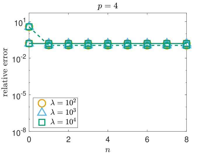
(a)

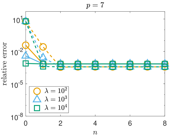
(b)

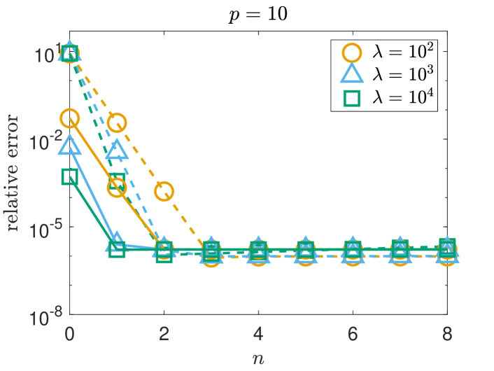
(c)

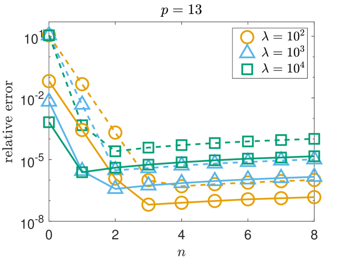
(d)

Figure 1: Relative velocity error (solid lines) and pressure error (dashed lines) of the solution $(\bm{u}_{X}^{n},p_{X}^{n})$ given by the SCIP method with (a) $p=4$, (b) $p=7$, (c) $p=10$, and (d) $p=13$ applied to the Kovasznay flow problem with $\nu=10^{-1}$.

We begin by examining the performance of SCIP using the 4x4 criss-cross mesh in Fig. 2(b). For $p\in\{4,7,10,13\}$, $\lambda\in\{10^{2},10^{3},10^{4}\}$, and $0\leq n\leq 8$, we terminate SCIP after $n$ steps and display the relative velocity error $\|\bm{u}-\bm{u}_{X}^{n}\|_{1}/\|\bm{u}\|_{1}$ and relative pressure error $\|q-q_{X}^{n}\|/\|q\|$ in Fig. 1. The relative errors are in agreement with Theorem 4.8. The errors decrease until the error in the SCIP method is smaller than the discretization error, at which point the errors level off. Additionally, the pressure errors generally require one to two more iterations of SCIP to level off compared to the velocity errors.

Figure 2(a) shows the behavior of the velocity and pressure errors versus the polynomial degree on a log-linear scale so that a straight line corresponds to the expected exponential convergence in $p$ since the exact solution Eq. 38 is analytic [19]. Observe that, while we indeed see exponential convergence for $p\in\{1,\ldots,10\}$, for higher values of $p$ there is a loss in accuracy which we attribute to the conditioning of the Bernstein basis.

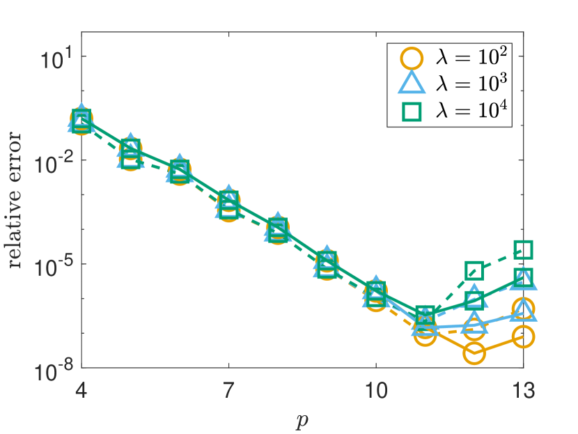
(a)

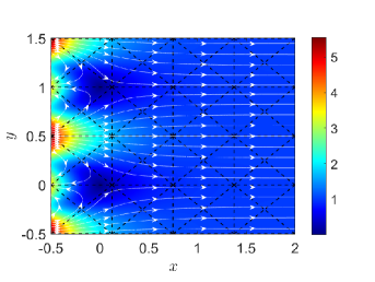
(b)

Figure 2: SCIP approximation to the Kovasznay flow problem with $\nu=10^{-1}$. (a) Smallest relative velocity error (solid lines) and pressure error (dashed lines) of the solution $(\bm{u}_{X}^{n},p_{X}^{n})$ over 8 iterations and (b) 4x4 criss-cross mesh (dashed lines) and velocity streamlines (solid lines) with $|\bm{u}_{X}^{n}|$ background color for the $p=10$ and $\lambda=10^{3}$ approximation after 8 iterations.

The divergence of the SCIP approximation $\|\operatorname{div}\bm{u}_{X}^{n}\|$ is another important quantity that, according to Theorem 4.8, converges exponentially fast as the number of iterations increases. The values of $\|\operatorname{div}\bm{u}_{X}^{n}\|$ for the same values of $n$ and $p$ in Fig. 1 are displayed in Fig. 3, where in agreement with Eq. 35, $\|\operatorname{div}\bm{u}_{X}^{n}\|$, and hence $\|\operatorname{div}\tilde{\bm{u}}^{n}\|$, decays exponentially fast in $n$, and the rate of decay is greater for larger values of $\lambda$. We observe some degradation of the results when $p>10$, which we again attribute to roundoff issues with the Bernstein basis. The approximation obtained after 8 iterations of SCIP with $p=10$ and $\lambda=10^{3}$ is displayed in Fig. 2(b).

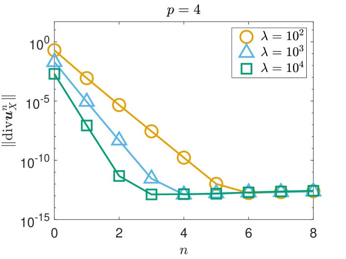
(a)

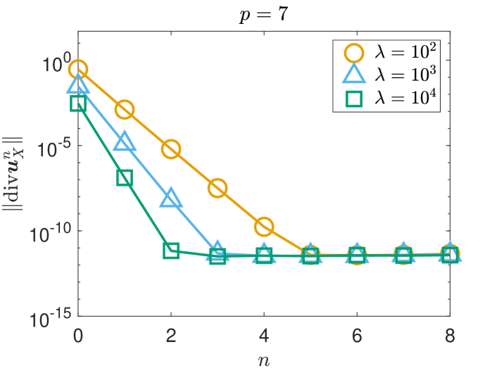
(b)

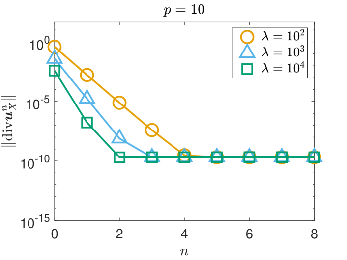
(c)

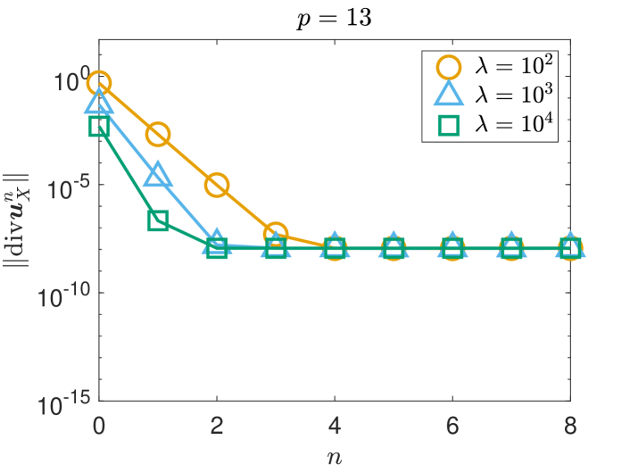
(d)

Figure 3: Values of $\|\operatorname{div}\bm{u}_{X}^{n}\|$ with(a) $p=4$, (b) $p=7$, (c) $p=10$, and (d) $p=13$ from the SCIP method applied to the Kovasznay flow problem with $\nu=10^{-1}$.

5.3 Moffatt Eddies

We now consider an example of Stokes flow due to Moffatt [14], which is a common benchmark for high order methods as it contains features on many scales. Let $\Omega$ be the wedge with a fixed mesh as shown in Fig. 4(a) with the following boundary conditions:

$$\bm{u}(x,0)=\begin{bmatrix}1-x^{2}\\ 0\end{bmatrix},\qquad-1\leq x\leq 1,\quad\text{and}\quad\bm{u}=\bm{0}\text{ on }\Gamma\setminus(-1,1)\times\{0\}.$$

The velocity contains an infinite cascade of eddies, each of which is about 400 times weaker than the previous one, while the pressure has an infinite cascade of singularities, starting at $(\pm 1,0)$. The combination of these two features makes this a challenging test problem.

(a)

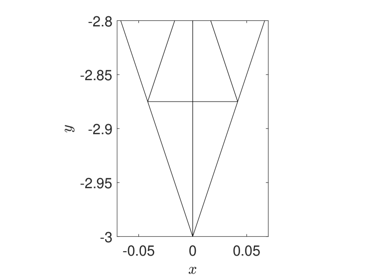
(b)

Figure 4: (a) Computational mesh consisting of 22 elements and (b) zoom for the Moffatt problem.

The numerical solution obtained after 8 iterations of the SCIP method with $p=10$ and $\lambda=10^{3}$ on the computational mesh in Fig. 4(a) satisfies $\|\operatorname{div}\bm{u}_{X}^{n}\|=$ 6.8e-11 and is shown in Fig. 5. Observe that the method nicely captures the profile of the pressure, as well as the three eddies. In Fig. 6, we zoom in on the numerical solution and observe that an additional two eddies are resolved, with $|\bm{u}_{X}^{n}|$ being on the order of $10^{-11}$. Thus, the method is able to resolve all eddies up to the order of $\|\operatorname{div}\bm{u}_{X}^{n}\|$ and capture the pressure profile without the need to use a priori knowledge of the solution.

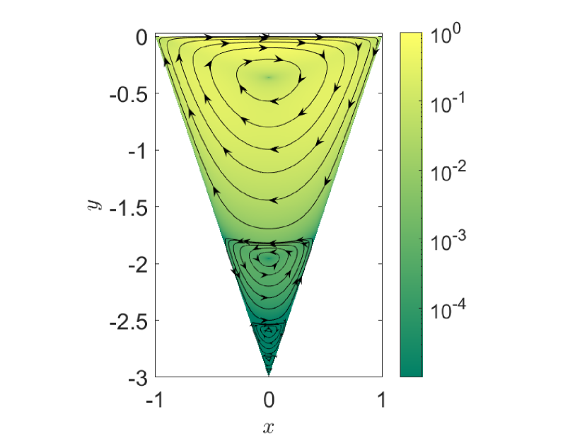
(a)

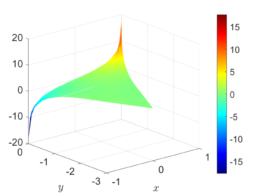
(b)

Figure 5: SCIP approximation of the Moffatt problem with $p=10$ and $\lambda=10^{3}$: (a) velocity streamlines with $|\bm{u}|$ background color and (b) pressure.

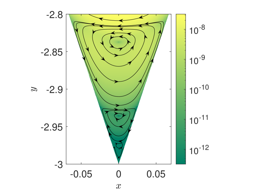
(a)

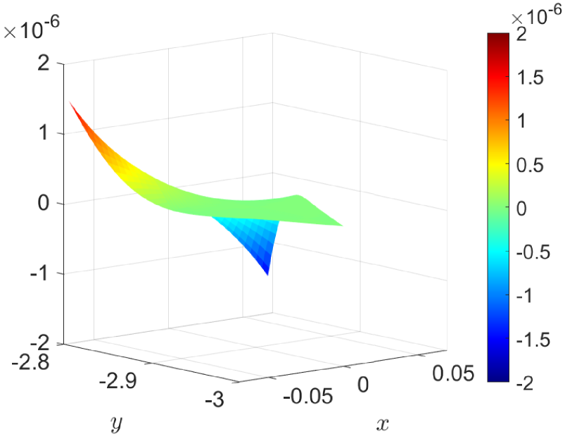
(b)

Figure 6: Zoom on bottom eddies of the SCIP approximation of the Moffatt problem with $p=10$ and $\lambda=10^{3}$: (a) velocity streamlines with $|\bm{u}|$ background color and (b) pressure.

6 Stokes Extension Operators

Given a function $\bm{u}\in\bm{X}:=X\times X$ and $K\in\mathcal{T}$, Lemma 4.1 shows that there exists a unique $(\bm{u}_{S,K},q_{S,K})\in\bm{\mathcal{P}}_{p}(K)\times\operatorname{div}\bm{X}_{I}(K)$ satisfying

(39a) $$a_{K}(\bm{u}_{S,K},\bm{v})-(q_{S,K},\operatorname{div}\bm{v})_{K} =0\qquad \forall\bm{v}\in\bm{X}_{I}(K),$$

(39b) $$-(r,\operatorname{div}\bm{u}_{S,K})_{K} =0\qquad \forall r\in\operatorname{div}\bm{X}_{I}(K),$$

(39c) $$(\bm{u}_{S,K}-\bm{u})|_{\partial K} =\bm{0}.\qquad$$

We define the discrete Stokes extension operators $\mathbb{S}:\bm{X}\to\bm{X}$ and $\mathbb{Q}:\bm{X}\to\operatorname{div}\bm{X}_{I}$ by the rules $\mathbb{S}\bm{u}|_{K}:=\bm{u}_{S,K}$ and $\mathbb{Q}\bm{u}|_{K}=q_{S,K}$ for all $K\in\mathcal{T}$. Similarly, there exist $\bm{u}_{S,K}^{\dagger}\in\bm{\mathcal{P}}_{p}(K)$ and $q_{S,K}^{\dagger}\in\operatorname{div}\bm{X}_{I}(K)$ satisfying

(40) $$a_{K}(\bm{v},\bm{u}_{S,K}^{\dagger})-(q_{S,K}^{\dagger},\operatorname{div}\bm{v})_{K} =0\qquad\forall\bm{v}\in\bm{X}_{I}(K),$$

along with Eq. 39b, and Eq. 39c. We define the “adjoint” Stokes extension operators $\mathbb{S}^{\dagger}$ and $\mathbb{Q}^{\dagger}$ in terms of $\bm{u}_{S,K}^{\dagger}$ and $q_{S,K}^{\dagger}$ analogously.

The next result gives a precise statement of the sense in which the above operators are “adjoints.” Let $s(\cdot,\cdot;\cdot,\cdot)$ denote the Stokes bilinear form

$$s(\bm{u},q;\bm{v},r):=a(\bm{u},\bm{v})-(q,\operatorname{div}\bm{v})-(r,\operatorname{div}\bm{u})\qquad\forall\bm{u},\bm{v}\in\bm{X},\ \forall q,r\in\operatorname{div}\bm{X}.$$

Additionally, let $\Pi_{I}:L^{2}(\Omega)\to\operatorname{div}\bm{X}_{I}$ denote the usual $L^{2}(\Omega)$ projection operator onto $\operatorname{div}\bm{X}_{I}$:

$$(\Pi_{I}q,r)=(q,r)\qquad\forall q\in L^{2}(\Omega),\ \forall r\in\operatorname{div}\bm{X}_{I},$$

and $\Pi_{I}^{\perp}:=I-\Pi_{I}$. Then, we have the following result:

Lemma 6.1.

For all $\bm{u},\bm{v}\in\bm{X}$ and $q,r\in\operatorname{div}\bm{X}$, there holds

(41) $$s(\mathbb{S}\bm{u},\mathbb{Q}\bm{u}+\Pi_{I}^{\perp}q;\bm{v},r)=s(\bm{u},q;\mathbb{S}^{\dagger}\bm{v},\mathbb{Q}^{\dagger}\bm{v}+\Pi_{I}^{\perp}r)$$

and

(42) $$\operatorname{div}\mathbb{S}\bm{u}=\operatorname{div}\mathbb{S}^{\dagger}\bm{u}=\Pi_{I}^{\perp}\operatorname{div}\bm{u}.$$

Proof 6.2.

Let $\bm{u}\in\bm{X}$ be given. Then, $\bm{u}_{I}:=\bm{u}-\mathbb{S}\bm{u}$ satisfies $\bm{u}_{I}\in\bm{X}_{I}$ by Eq. 39c, and so $\operatorname{div}\mathbb{S}\bm{u}=\operatorname{div}\bm{u}+\operatorname{div}\bm{u}_{I}$. Applying $\Pi_{I}^{\perp}$ gives

$$\operatorname{div}\mathbb{S}\bm{u}=\Pi_{I}^{\perp}\operatorname{div}\mathbb{S}\bm{u}=\Pi_{I}^{\perp}\operatorname{div}\bm{u}+\Pi_{I}^{\perp}\operatorname{div}\bm{u}_{I}=\Pi_{I}^{\perp}\operatorname{div}\bm{u},$$

where we used Eq. 39b and that $\Pi_{I}\operatorname{div}\bm{u}_{I}=\operatorname{div}\bm{u}_{I}$. Similar arguments show that $\operatorname{div}\mathbb{S}^{\dagger}\bm{u}=\Pi_{I}^{\perp}\operatorname{div}\bm{u}$, and Eq. 42 follows.

Now let $\bm{u},\bm{v}\in\bm{X}$ and $q,r\in\operatorname{div}\bm{X}$ be given. Thanks to Eq. 42, there holds

$$(\Pi_{I}^{\perp}q,\operatorname{div}\bm{v})+(r,\operatorname{div}\mathbb{S}\bm{u}) =(q,\Pi_{I}^{\perp}\operatorname{div}\bm{v})+(r,\Pi_{I}^{\perp}\operatorname{div}\bm{u})$$

$$=(q,\operatorname{div}\mathbb{S}^{\dagger}\bm{v})+(\Pi_{I}^{\perp}r,\operatorname{div}\bm{u}),$$

and so

$$s(\mathbb{S}\bm{u},\mathbb{Q}\bm{u}+\Pi_{I}^{\perp}q;\bm{v},r)=a(\mathbb{S}\bm{u},\bm{v})-(\mathbb{Q}\bm{u},\operatorname{div}\bm{v})-(q,\operatorname{div}\mathbb{S}^{\dagger}\bm{v})-(\Pi_{I}^{\perp}r,\operatorname{div}\bm{u}).$$

Since $\bm{v}-\mathbb{S}^{\dagger}\bm{v}\in\bm{X}_{I}$ by Eq. 39c, we have

$$a(\mathbb{S}\bm{u},\bm{v})-(\mathbb{Q}\bm{u},\operatorname{div}\bm{v})=a(\mathbb{S}\bm{u},\mathbb{S}^{\dagger}\bm{v})-(\mathbb{Q}\bm{u},\operatorname{div}\mathbb{S}^{\dagger}\bm{v})=a(\mathbb{S}\bm{u},\mathbb{S}^{\dagger}\bm{v}),$$

where we used Eq. 39a and Eq. 39b. Applying similar arguments to $\bm{u}-\mathbb{S}\bm{u}$ gives

$$a(\mathbb{S}\bm{u},\mathbb{S}^{\dagger}\bm{v})=a(\bm{u},\mathbb{S}^{\dagger}\bm{v})+(\mathbb{Q}^{\dagger}\bm{v},\operatorname{div}(\mathbb{S}\bm{u}-\bm{u}))=a(\bm{u},\mathbb{S}^{\dagger}\bm{v})-(\mathbb{Q}^{\dagger}\bm{v},\operatorname{div}\bm{u}),$$

where we used Eq. 40 and Eq. 39b. Equation 41 now follows on collecting results.

The next result characterizes $\tilde{\bm{X}}_{B}$ as an invariant subspace of $\bm{X}_{D}$ under the operator $\mathbb{S}$ and likewise for $\tilde{\bm{X}}_{B}^{\dagger}$ and $\mathbb{S}^{\dagger}$:

Lemma 6.3.

The following identities holds:

(43) $$\tilde{\bm{X}}_{B} =\{\bm{v}\in\bm{X}_{D}:\mathbb{S}\bm{v}=\bm{v}\}=\{\mathbb{S}\bm{v}:\bm{v}\in\bm{X}_{D}\},$$

(44) $$\tilde{\bm{X}}_{B}^{\dagger} =\{\bm{v}\in\bm{X}_{D}:\mathbb{S}^{\dagger}\bm{v}=\bm{v}\}=\{\mathbb{S}^{\dagger}\bm{v}:\bm{v}\in\bm{X}_{D}\}.$$

Moreover,

(45) $$\operatorname{div}\tilde{\bm{X}}_{B}=\operatorname{div}\tilde{\bm{X}}_{B}^{\dagger}.$$

Proof 6.4.

Let $\bm{u}\in\bm{X}_{D}$ and $K\in\mathcal{T}$. Using the notation of Section 4, $\bm{u}|_{K}$ may be expressed as $\bm{u}|_{K}=\vec{\Phi}_{B,K}^{T}\vec{u}_{B,K}+\vec{\Phi}_{I,K}^{T}\vec{u}_{I,K}$. By Eq. 39, $\mathbb{S}\bm{u}|_{K}=\vec{\Phi}_{B,K}^{T}\vec{u}_{B,K}+\vec{\Phi}_{I,K}^{T}\vec{u}_{I,K}^{\#}$, where

$$\begin{bmatrix}\bm{E}_{II}&\bm{G}_{\iota I}^{T}\\ \bm{G}_{\iota I}&\bm{0}\end{bmatrix}\begin{bmatrix}\vec{u}_{I,K}^{\#}\\ *\end{bmatrix}=-\begin{bmatrix}\bm{E}_{IB}\\ \bm{G}_{\iota B}\end{bmatrix}\vec{u}_{B,K}.$$

Thus, $\{\bm{v}\in\bm{X}_{D}:\mathbb{S}\bm{v}=\bm{v}\}=\{\mathbb{S}\bm{v}:\bm{v}\in\bm{X}_{D}\}=\{\bm{v}\in\bm{X}_{D}:\vec{v}_{I,K}=\bm{S}_{K}\vec{v}_{B,K}\ \forall K\in\mathcal{T}\}$, and so Eq. 43 follows from Lemma 4.3. Similar arguments give Eq. 44. Equation 45 is now a consequence of Eq. 42.

Lemma 6.5.

For all $\bm{u},\bm{v}\in\bm{X}$, there holds

(46) $$a(\mathbb{S}\bm{u},\mathbb{S}\bm{v})=a(\mathbb{S}\bm{u},\mathbb{S}^{\dagger}\bm{v})=a(\mathbb{S}^{\dagger}\bm{u},\mathbb{S}^{\dagger}\bm{v}).$$

Proof 6.6.

Let $\bm{u},\bm{v}\in\bm{X}$. By Eqs. 42 and 39c, $\mathbb{S}\bm{u}-\mathbb{S}^{\dagger}\bm{u},\mathbb{S}\bm{v}-\mathbb{S}^{\dagger}\bm{v}\in\bm{N}_{I}$, and so

$$a(\mathbb{S}\bm{u},\mathbb{S}\bm{v}) =a(\mathbb{S}\bm{u},\mathbb{S}^{\dagger}\bm{v})+a(\mathbb{S}\bm{u},\mathbb{S}\bm{v}-\mathbb{S}^{\dagger}\bm{v})=a(\mathbb{S}\bm{u},\mathbb{S}^{\dagger}\bm{v})$$

$$a(\mathbb{S}\bm{u},\mathbb{S}^{\dagger}\bm{v}) =a(\mathbb{S}^{\dagger}\bm{u},\mathbb{S}^{\dagger}\bm{v})+a(\mathbb{S}\bm{u}-\mathbb{S}^{\dagger}\bm{u},\bm{v})=a(\mathbb{S}^{\dagger}\bm{u},\mathbb{S}^{\dagger}\bm{v})$$

by Eq. 39a with $\bm{v}=\mathbb{S}\bm{v}-\mathbb{S}^{\dagger}\bm{v}$ and Eq. 40 with $\bm{v}=\mathbb{S}\bm{u}-\mathbb{S}^{\dagger}\bm{u}$.

Lemma 6.7.

Let $\tilde{\bm{N}}_{B}:=\{\bm{z}\in\tilde{\bm{X}}_{B}:\operatorname{div}\bm{z}\equiv 0\}$ and $\tilde{\bm{N}}_{B}^{\dagger}:=\{\bm{z}\in\tilde{\bm{X}}_{B}^{\dagger}:\operatorname{div}\bm{z}\equiv 0\}$. The variational problem

(47) $$\bm{z}\in\tilde{\bm{N}}_{B}:\qquad a(\bm{z},\bm{w})=F(\bm{w})\qquad\forall\bm{w}\in\tilde{\bm{N}}_{B}^{\dagger}$$

is uniquely solvable for all linear functionals $F$ on $\tilde{\bm{N}}_{B}^{\dagger}$.

Proof 6.8.

Since Eq. 47 is equivalent to a square linear system, it suffices to show uniqueness. Suppose that $\bm{z}\in\tilde{\bm{N}}_{B}$ satisfies Eq. 47 with $F\equiv 0$. Choosing $\bm{w}=\mathbb{S}^{\dagger}\bm{z}$ and applying Eq. 46 gives $a(\bm{z},\bm{z})=a(\bm{z},\mathbb{S}^{\dagger}\bm{z})=0$. By ellipticity Eq. 5, $\bm{z}\equiv 0$.

6.1 Proof of Lemma 4.7

Since Eq. 31 is equivalent to a square linear system, it again suffices to show uniqueness. Let $(\tilde{\bm{u}},\tilde{q})$ satisfy Eq. 31 with zero data on the RHS. Equations Eq. 31b and Eq. 45 means that $\operatorname{div}\tilde{\bm{u}}\equiv 0$ and so $\tilde{\bm{u}}\in\tilde{\bm{N}}_{B}$. Choosing $\bm{v}\in\tilde{\bm{N}}_{B}^{\dagger}$ in Eq. 31a shows that $\tilde{\bm{u}}$ satisfies Eq. 47 with $F\equiv 0$. By Lemma 6.7, $\tilde{\bm{u}}\equiv 0$.

Thanks to Eq. 45, there exists $\bm{v}\in\tilde{\bm{X}}_{B}^{\dagger}$ such that $\operatorname{div}\bm{v}=\tilde{q}$. Substituting this choice into Eq. 31a gives $\|\tilde{q}\|^{2}=(\tilde{q},\operatorname{div}\bm{v})=0$, and so $\tilde{q}\equiv 0$. Thus, Eq. 31 is uniquely solvable. Moreover, for each $K\in\mathcal{T}$, there exists $(\bm{u}_{K},q_{K})\in\bm{X}_{I}(K)\times\operatorname{div}\bm{X}_{I}(K)$ satisfying Eq. 32 by Lemma 4.1.

By Eq. 32, the functions $\bm{u}_{I}:=\sum_{K\in\mathcal{T}}\bm{u}_{K}$ and $q_{I}:=\sum_{K\in\mathcal{T}}q_{K}$ satisfy

(48a) $$a(\bm{u}_{I},\bm{v})-(q_{I},\operatorname{div}\bm{v}) =L(\bm{v})-a(\tilde{\bm{u}},\bm{v})\qquad \forall\bm{v}\in\bm{X}_{I},$$

(48b) $$-(r,\operatorname{div}\bm{u}_{I}) =0\qquad \forall r\in\operatorname{div}\bm{X}_{I}.$$

Let $\bm{u}_{X}:=\tilde{\bm{u}}+\bm{u}_{I}$ and $q_{X}:=\tilde{q}+q_{I}$. Equation 31b means that $\operatorname{div}\tilde{\bm{u}}\equiv 0$, while relation Eq. 48b means that $\operatorname{div}\bm{u}_{I}\equiv 0$. As a result, $\operatorname{div}\bm{u}_{X}\equiv 0$ and so Eq. 7b is satisfied.

We now show that Eq. 7a holds. For $\bm{v}\in\bm{X}_{I}$, there holds

$$a(\bm{u}_{X},\bm{v})-(q_{X},\operatorname{div}\bm{v}) =a(\tilde{\bm{u}},\bm{v})+a(\bm{u}_{I},\bm{v})-(q_{I},\operatorname{div}\bm{v})=L(\bm{v}),$$

where we used Eq. 48a and that $(\tilde{q},\operatorname{div}\bm{v})=0$ by Eq. 22. For $\bm{v}\in\tilde{\bm{X}}_{B}^{\dagger}$, there holds

$$a(\bm{u}_{X},\bm{v})-(q_{X},\operatorname{div}\bm{v})=a(\tilde{\bm{u}},\bm{v})-(\tilde{q},\operatorname{div}\bm{v})+a(\bm{u}_{I},\bm{v})=L(\bm{v})+a(\bm{u}_{I},\bm{v}),$$

where we used Eq. 31a and that $(q_{I},\operatorname{div}\bm{v})=0$ by Eq. 22. Since $\bm{v}\in\tilde{\bm{X}}_{B}^{\dagger}$ and $\operatorname{div}\bm{u}_{I}\equiv 0$, $a(\bm{u}_{I},\bm{v})=0$ by definition. Equation 7a now follows from linearity thanks to the decomposition Eq. 29 with $\tilde{\bm{X}}_{B}^{\dagger}$.

7 Convergence of SCIP and the Iterated Penalty Method

We begin with an estimate for functions in $\tilde{\bm{X}}_{B}$ that are orthogonal to divergence free functions:

Lemma 7.1.

Let $\tilde{\bm{N}}_{B}^{\perp}:=\{\bm{v}\in\tilde{\bm{X}}_{B}:a(\bm{v},\bm{z})=0\ \forall\bm{z}\in\tilde{\bm{N}}_{B}^{\dagger}\}$. Then,

(49) $$\|\bm{u}\|_{1}\leq\frac{(M+\alpha)^{2}}{\alpha^{2}\beta_{X}}\|\operatorname{div}\bm{u}\|\qquad\forall\bm{u}\in\tilde{\bm{N}}_{B}^{\perp},$$

where $M>0$ Eq. 4, $\alpha>0$ Eq. 5, and $\beta_{X}>0$ Eq. 8.

Proof 7.2.

Let $\bm{u}\in\tilde{\bm{N}}_{B}^{\perp}$. By the proof of Theorem 4.5, there exists $\bm{v}\in\tilde{\bm{X}}_{B}$ such that $\operatorname{div}\bm{v}=\operatorname{div}\bm{u}$ and $\|\bm{v}\|_{1}\leq(M+\alpha)(\alpha\beta_{X})^{-1}\|\operatorname{div}\bm{u}\|$. Since Eq. 47 is uniquely solvable by Lemma 6.7, there exists $\bm{z}\in\tilde{\bm{N}}_{B}$ such that $a(\bm{z},\bm{n})=a(\bm{v},\bm{n})$ for all $\bm{n}\in\tilde{\bm{N}}_{B}^{\dagger}$. By ellipticity Eq. 5 and Eq. 46, we have

$$\alpha\|\bm{z}\|_{1}^{2}\leq a(\bm{z},\bm{z})=a(\bm{z},\mathbb{S}^{\dagger}\bm{z})=a(\bm{v},\mathbb{S}^{\dagger}\bm{z})=a(\bm{v},\bm{z})\leq M\|\bm{v}\|_{1}\|\bm{z}\|_{1},$$

since $\mathbb{S}\bm{z}=\bm{z}$ by Lemma 6.3. Thus, $\|\bm{z}\|_{1}\leq M\alpha^{-1}\|\bm{v}\|_{1}$.

Let $\bm{w}:=\bm{v}-\bm{z}$. By construction, $\operatorname{div}\bm{w}=\operatorname{div}\bm{u}$ and $\bm{w}\in\tilde{\bm{N}}_{B}^{\perp}$. Moreover, $\bm{w}$ satisfies Eq. 49 thanks to the triangle inequality. To complete the proof, we now show that $\bm{u}=\bm{w}$. Since $\operatorname{div}(\bm{u}-\bm{w})=0$, there exists $\bm{e}:=\bm{u}-\bm{w}\in\tilde{\bm{N}}_{B}^{\perp}$. Thanks to Eq. 46, $0=a(\bm{e},\mathbb{S}^{\dagger}\bm{e})=a(\bm{e},\bm{e})\geq\alpha\|\bm{e}\|_{1}^{2}$. Consequently, $\bm{e}\equiv\bm{0}$ and so $\bm{u}=\bm{w}$.

With Lemma 7.1 in hand, the proof of Theorem 4.8 is a generalization of the convergence proof for the standard iterated penalty method (see e.g. [6, p.356-359]).

Proof 7.3 (Proof of Theorem 4.8).

Let $\bm{e}^{n}:=\tilde{\bm{u}}-\tilde{\bm{u}}^{n}$ and $r^{n}:=\tilde{q}-\tilde{q}^{n}$, $n\in\mathbb{N}_{0}$. Subtracting Eq. 36 from Eq. 31a gives, for $n\in\mathbb{N}_{0}$,

(50) $$a_{\lambda}(\bm{e}^{n},\bm{v}) =(r^{n},\operatorname{div}\bm{v})\qquad\forall\bm{v}\in\bm{X}_{B}^{\dagger}$$

and $r^{n+1}=r^{n}+\lambda\operatorname{div}\tilde{\bm{u}}^{n}=r^{n}-\lambda\operatorname{div}\bm{e}^{n}$ since $\operatorname{div}\tilde{\bm{u}}=0$. Using these relations, we obtain

$$a_{\lambda}(\bm{e}^{n+1},\bm{v}) =(r^{n},\operatorname{div}\bm{v})-\lambda(\operatorname{div}\bm{e}^{n},\operatorname{div}\bm{v})=a_{\lambda}(\bm{e}^{n},\bm{v})-\lambda(\operatorname{div}\bm{e}^{n},\operatorname{div}\bm{v})=a(\bm{e}^{n},\bm{v})$$

for all $\bm{v}\in\tilde{\bm{X}}_{B}^{\dagger}$. Choosing $\bm{v}=\mathbb{S}^{\dagger}\bm{e}^{n+1}$ and using Eqs. 46 and 42 then gives

(51) $$a(\bm{e}^{n+1},\bm{e}^{n+1})+\lambda\|\operatorname{div}\bm{e}^{n+1}\|^{2}=a(\bm{e}^{n},\mathbb{S}^{\dagger}\bm{e}^{n+1})=a(\bm{e}^{n},\bm{e}^{n+1})\leq M\|\bm{e}^{n}\|_{1}\|\bm{e}^{n+1}\|_{1},$$

where we used Eq. 46 and that $\mathbb{S}\bm{e}^{n+1}=\bm{e}^{n+1}$. Moreover, Eq. 50 shows that $\bm{e}^{n+1}\in\tilde{\bm{N}}_{B}^{\perp}$ for all $n\in\mathbb{N}_{0}$. Applying Lemma 7.1 and Eq. 5 to the LHS of Eq. 51 gives

(52) $$(\alpha+\lambda\tilde{\Upsilon}^{-2})\|\bm{e}^{n+1}\|_{1}\leq M\|\bm{e}^{n}\|_{1}\implies\|\bm{e}^{n}\|_{1}\leq(M\tilde{\Upsilon}^{2}\lambda^{-1})^{n}\|\bm{e}^{0}\|_{1},$$

where $\tilde{\Upsilon}:=(M+\alpha)^{2}/(\alpha^{2}\beta_{X})$, the constant appearing in Eq. 49. Equation 35 now follows from Eq. 52 on noting that $\operatorname{div}\tilde{\bm{u}}^{n}=-\operatorname{div}\bm{e}^{n}$.

Now, we use Lemma 7.1 to obtain

(53) $$\|\bm{e}^{n}\|\leq\tilde{\Upsilon}\|\operatorname{div}\bm{e}^{n}\|=\tilde{\Upsilon}\|\operatorname{div}\tilde{\bm{u}}^{n}\|.$$

Applying the inf-sup condition Eq. 30 for $\tilde{\bm{X}}_{B}^{\dagger}\times\operatorname{div}\tilde{\bm{X}}_{B}^{\dagger}$ and using Eqs. 50 and 45 gives

$$\tilde{\beta}_{X}\|r^{n}\|\leq\sup_{\bm{0}\neq\bm{v}\in\tilde{\bm{X}}_{B}^{\dagger}}\frac{(r^{n},\operatorname{div}\bm{v})}{\|\bm{v}\|_{1}}=\sup_{\bm{0}\neq\bm{v}\in\tilde{\bm{X}}_{B}^{\dagger}}\frac{a_{\lambda}(\bm{e}^{n},\bm{v})}{|\bm{v}|_{1}}\leq M\|\bm{e}^{n}\|_{1}+\sqrt{d}\lambda\|\operatorname{div}\bm{e}^{n}\|,$$

where $\tilde{\beta}_{X}:=\alpha\beta_{X}(M+\alpha)^{-1}$. Thanks to Eq. 53, $\|r^{n}\|\leq(M\tilde{\Upsilon}+\sqrt{d}\lambda)\tilde{\beta}_{X}^{-1}\|\operatorname{div}\tilde{\bm{u}}^{n}\|$. Equation 34 now follows on collecting results.

7.1 Convergence of the Standard IP Method

The following result, which is an immediate consequence of [6, eq. (13.1.16)], is the analogue of Lemma 7.1:

Lemma 7.4.

For all $\bm{u}\in\{\bm{v}\in\bm{X}_{D}:a(\bm{v},\bm{w})=0\ \forall\bm{w}\in\bm{X}_{D}:\operatorname{div}\bm{w}=0\}$, there holds

$$\|\bm{u}\|_{1}\leq\frac{M+\alpha}{\alpha\beta_{X}}\|\operatorname{div}\bm{u}\|,$$

where $M>0$ Eq. 4, $\alpha>0$ Eq. 5, and $\beta_{X}>0$ Eq. 8.

With Lemma 7.4 in hand, the proof of Theorem 3.1 is analogous to the proof of Theorem 4.8: the spaces $\tilde{\bm{X}}_{B}$ and $\tilde{\bm{X}}_{B}^{\dagger}$ are replaced by $\bm{X}_{D}$; the choice $\bm{v}=\mathbb{S}^{\dagger}\bm{e}^{n+1}$ is replaced by $\bm{v}=\bm{e}^{n+1}$; the use of Lemma 7.1 and $\tilde{\Upsilon}$ are replaced by Lemma 7.4 and $\Upsilon:=(M+\alpha)/(\alpha\beta_{X})$; and the inf-sup constant $\tilde{\beta}_{X}$ is replaced by $\beta_{X}$ defined in Eq. 8.

Appendix A Properties of the 2D Scott-Vogelius Elements

(a)

(b)

Figure 7: Notation for mesh around (a) an internal vertex $\bm{a}\in\mathcal{V}_{I}$ and (b) a boundary vertex $\bm{a}\in\mathcal{V}_{D}$, each abutting $m=|\mathcal{T}_{\bm{a}}|$ elements.

Finally, in this section, we turn to the the fundamental stability and approximation properties of the 2D Scott-Vogelius elements, as well as discrete exact sequence properties. One of the key conditions for optimal approximation properties is that the mesh is corner-split at Dirichlet vertices. Roughly speaking, a mesh is corner-split if every element has at most one edge lying on $\Gamma_{D}$. In order to give a precise definition, we let $\mathcal{V}$ denote the set of element vertices, $\mathcal{V}_{I}$ the set of interior vertices, and $\mathcal{V}_{C}$ the set of element vertices coinciding with the corners of the physical domain $\Omega$. For $\bm{a}\in\mathcal{V}_{I}\cup\mathcal{V}_{D}$, we label the elements as in Fig. 7 and define

(54) $$\xi(\bm{a}):=\sum_{i=1}^{|\mathcal{T}_{\bm{a}}|-\eta_{\bm{a}}}|\sin(\theta_{i}+\theta_{i+1})|,\qquad\text{where }\eta_{\bm{a}}=\begin{cases}1&\bm{a}\in\mathcal{V}_{D},\\ 0&\bm{a}\in\mathcal{V}_{I}.\end{cases}$$

A mesh is corner-split at Dirichlet vertices if $\{\bm{a}\in\mathcal{V}_{C}\cap\mathcal{V}_{D}:\xi(\bm{a})=0\}=\emptyset$.

The following result states that the 2D Scott-Vogelius elements are uniformly inf-sup stable in $h$ and $p$ and possess optimal approximation properties under mild assumptions on the mesh:

Theorem A.1.

Suppose that $p\geq 4$ and that the family of meshes $\{\mathcal{T}\}$ is corner-split at Dirichlet vertices and satisfies [5, eq. (5.14)]. Then, the Scott-Vogelius elements are uniformly inf-sup stable in $h$ and $p$; i.e., there exists $\beta>0$ independent of $h$ and $p$ such that

(55) $$\beta\|q\|\leq\sup_{\bm{0}\neq\bm{v}\in\bm{X}_{D}}\frac{(\operatorname{div}\bm{v},q)}{\|\bm{v}\|_{1}}\qquad\forall q\in\operatorname{div}\bm{X}_{D}.$$

Moreover, for $\bm{u}\in\bm{H}^{s}(\Omega)\cap\bm{H}^{1}_{D}(\Omega)$ and $q\in H^{s-1}(\Omega)\cap L^{2}_{D}(\Omega)$, $s>1$, there holds

(56) $$\inf_{\bm{v}\in\bm{X}_{D}}\|\bm{u}-\bm{v}\|_{1} \leq Ch^{\min(p,s-1)}p^{-(s-1)}\|\bm{u}\|_{s},$$

(57) $$\inf_{r\in\operatorname{div}\bm{X}_{D}}\|q-r\| \leq Ch^{\min(p,s-1)}p^{-(s-1)}\|q\|_{s-1},$$

where $C$ is independent of $\bm{u}$, $q$, $h$, and $p$.

The conditions needed in Theorem A.1 are quite standard, apart from the requirement that the mesh be corner-split at Dirichlet vertices. We refer to [5, p. 35] for a detailed characterization of the remaining mesh conditions in Theorem A.1 and assume they hold for the remainder of this paper. Although some progress on barycenter-refined meshes [24] and uniform tetrahedral grids [25] have been made for the 3D Scott-Vogelius elements, their stability, approximation, and exact sequence properties remain open.

The proof of Theorem A.1 is given in Section A.1. The inf-sup condition Eq. 8 with $\beta$ replaced by $Cp^{-K}$ for $p$ and $K>0$ sufficiently large, was shown in [23] – the restriction on the polynomial degree was subsequently relaxed to $p\geq 4$ in [21]. Here, we show that the elements are uniformly stable in both $h$ and $p$. Even though (optimal) approximation properties of the space $\bm{X}_{D}$ expressed in Eq. 56 are a consequence of standard approximation theory for $hp$-finite elements [19], the result Eq. 57 on the optimal approximability of the space $\operatorname{div}\bm{X}_{D}$ is also new, although the result was known for the pure traction problem ($|\Gamma_{D}|=0$) on a fixed mesh [22, Lemma 3.3]. Only one other conforming finite element discretization on (again corner-split) triangular meshes is known to be uniformly inf-sup stable in $h$ and $p$ and possess optimal approximation properties [2, 3].

A.1 Exact Sequence Properties

Let $\{\Gamma_{D,j}\}_{j=1}^{J}$ denote the connected components of $\Gamma_{D}$ and define

$$H^{2}_{D}(\Omega) :=\{\psi\in H^{2}(\Omega):\psi|_{\Gamma_{D,1}}=0,\ \text{$\psi|_{\Gamma_{D,j}}$ is constant, $2\leq j\leq J$, $\partial_{n}\psi|_{\Gamma_{D}}=0$}\}.$$

It is not difficult to see that $\operatorname{\mathbf{curl}}H^{2}_{D}(\Omega)\subset\bm{H}^{1}_{D}(\Omega)$ and $\operatorname{div}\bm{H}^{1}_{D}(\Omega)\subseteq L^{2}_{D}(\Omega)$, where $\operatorname{\mathbf{curl}}\phi=(\partial_{y}\phi,-\partial_{x}\phi)^{T}$. In fact, the following sequence is exact [18, Lemma 4.6.1] in the sense that the kernel of each operator appearing in Eq. 58 equals the range of the previous operator in the sequence:

(58) $$0\xrightarrow{\ \ \ \subset\ \ \ }H^{2}_{D}(\Omega)\xrightarrow{\ \ \operatorname{\mathbf{curl}}\ \ }\bm{H}^{1}_{D}(\Omega)\xrightarrow{\ \ \operatorname{div}\ \ }L^{2}_{D}(\Omega)\xrightarrow{\ \ \ 0\ \ \ }0.$$

For instance, if $\bm{u}\in\bm{H}^{1}_{D}(\Omega)$ is the velocity in Eq. 1 so that $\operatorname{div}\bm{u}\equiv 0$, then there exists a potential $\phi\in H^{2}_{D}(\Omega)$ such that $\bm{u}=\operatorname{\mathbf{curl}}\phi$.

We will show that the Scott-Vogelius finite element spaces $\bm{X}_{D}$ and $\operatorname{div}\bm{X}_{D}$ also form part of an exact sequence. To this end, define a discrete potential space by

$$\Sigma_{D}=\Sigma\cap H^{2}_{D}(\Omega),\qquad\text{where}\quad\Sigma:=\{\psi\in C^{1}(\bar{\Omega}):\psi|_{K}\in\mathcal{P}_{p+1}(K)\ \forall K\in\mathcal{T}\}.$$

As shown in [5, 21, 23], the space $\operatorname{div}\bm{X}_{D}$ satisfies a constraint at certain element vertices, which may be summarized as follows. Let $\mathcal{V}_{D}$ denote the set of element vertices lying on the interior of $\Gamma_{D}$ and $\mathcal{V}_{DN}$ denote the vertices coinciding with the intersection of $\bar{\Gamma}_{D}$ and $\bar{\Gamma}_{N}$. Additionally, given $\bm{a}\in\mathcal{V}$, let $\mathcal{T}_{\bm{a}}$ denote the set of elements sharing $\bm{a}$ as a vertex, labeled as in Fig. 7. Then, we have the following result:

Lemma A.2.

Let $\xi(\cdot)$ be defined as in Eq. 54 and define

$$Q :=\bigg{\{}q\in L^{2}(\Omega):q|_{K}\in\mathcal{P}_{p-1}(K)\ \forall K\in\mathcal{T},$$

$$\qquad\qquad\sum_{i=1}^{|\mathcal{T}_{\bm{a}}|}(-1)^{i}q|_{K_{i}}(\bm{a})=0\ \forall\bm{a}\in\mathcal{V}_{I}:\xi(\bm{a})=0\bigg{\}}$$

and

$$Q_{D} :=\bigg{\{}q\in Q\cap L^{2}_{D}(\Omega):\sum_{i=1}^{|\mathcal{T}_{\bm{a}}|}(-1)^{i}q|_{K_{i}}(\bm{a})=0\ \forall\bm{a}\in\mathcal{V}_{D}:\xi(\bm{a})=0\bigg{\}},$$

where the elements in $\mathcal{T}_{\bm{a}}$, $\bm{a}\in\mathcal{V}$, are labeled as in Fig. 7. Then, the sequence

(59) $$0\xrightarrow{\ \ \ \subset\ \ \ }\Sigma_{D}\xrightarrow{\ \ \operatorname{\mathbf{curl}}\ \ }\bm{X}_{D}\xrightarrow{\ \ \operatorname{div}\ \ }Q_{D}\xrightarrow{\ \ \ 0\ \ \ }0$$

is exact.

Proof A.3.

In the case $|\Gamma_{D}|=|\Gamma|$, Eq. 59 follows from the proof of Proposition 3.2 in [21], so we assume that $|\Gamma_{D}|<|\Gamma|$. The inclusion $\operatorname{\mathbf{curl}}\Sigma_{D}\subset\bm{X}_{D}$ follows by definition, while $\operatorname{div}\bm{X}_{D}=Q_{D}$ by [5, Theorem 4.1]. We may argue as in [16] and the proof of [18, Lemma 4.6.2] to show that

$$\dim\Sigma_{D}=\dim\Sigma-7|\mathcal{V}_{D}|-5|\mathcal{V}_{DN}|-(2p-7)|\mathcal{E}_{D}|+|\{\bm{a}\in\mathcal{V}_{D}:\xi(\bm{a})=0\}|+J-1,$$

where $\mathcal{E}_{D}$ is the set of element edges lying on $\Gamma_{D}$. Counting the constraints on the space $\bm{X}_{D}$ and $Q_{D}$ gives

$$\dim\bm{X}_{D} =\dim\bm{X}-2\left\{|\mathcal{V}_{D}|+|\mathcal{V}_{DN}|+(p-1)|\mathcal{E}_{D}|\right\}$$

$$\dim Q_{D} =\dim Q-|\{\bm{a}\in\mathcal{V}_{D}:\xi(\bm{a})=0\}|.$$

By [5, Lemma 6.1], $\dim\Sigma+\dim Q-\dim\bm{X}=1$, and so

$$\dim\Sigma_{D}+\dim Q_{D}-\dim\bm{X}_{D}=J-5|\mathcal{V}_{D}|-3|\mathcal{V}_{DN}|+5|\mathcal{E}_{D}|.$$

Moreover,

$$|\mathcal{E}_{D}|=\sum_{j=1}^{J}|\mathcal{E}_{D}\cap\Gamma_{D,j}|=\sum_{j=1}^{J}\left\{|(\mathcal{V}_{D}\cup\mathcal{V}_{DN})\cap\bar{\Gamma}_{D,j}|-1\right\}=|\mathcal{V}_{D}|+|\mathcal{V}_{DN}|-J,$$

where we used Euler’s identity on each connected component $\Gamma_{D,j}$: $|\mathcal{E}_{D}\cap\Gamma_{D,j}|=|(\mathcal{V}_{D}\cup\mathcal{V}_{DN})\cap\bar{\Gamma}_{D,j}|-1$. Additionally, the endpoints of each connected component $\Gamma_{D,j}$ consist of two unique vertices in $\mathcal{V}_{DN}$, and so $|\mathcal{V}_{DN}|=2J$. Collecting results, we have $\dim\Sigma_{D}+\dim Q_{D}-\dim\bm{X}_{D}=0.$ The exactness of Eq. 59 now follows using standard arguments (see e.g. [21, Proposition 3.1] or [5, Lemma 6.1]).

A.2 Stability and Approximation

With an explicit characterization $Q_{D}=\operatorname{div}\bm{X}_{D}$ thanks to Eq. 59 in hand, we now prove Theorem A.1.

Proof A.4 (Proof of Theorem A.1).

Equation 55 is an immediate consequence of [5, Theorem 5.1]. Let $\tilde{Q}_{D}:=\{r\in L^{2}_{D}(\Omega):r|_{K}\in\mathcal{P}_{p-1}(K)\ \forall K\in\mathcal{T}\text{ $r$ is continuous at}$ $\text{noncorner vertices}\}$.

By [3, Theorem 2.1], there holds

(60) $$\inf_{r\in\tilde{Q}_{D}}\|q-r\|\leq Ch^{\min(p,s-1)}p^{-(s-1)}\|q\|_{s-1},$$

where $C$ is independent of $h$ and $p$ in the case $L^{2}_{D}(\Omega)=L^{2}_{0}(\Omega)$. Exactly the same construction in [3, Lemmas 4.2 & 4.3] shows that Eq. 60 also holds in the case $L^{2}_{D}(\Omega)=L^{2}(\Omega)$. Since the mesh is corner-split at Dirichlet vertices, the set $\{\bm{a}\in\mathcal{V}_{I}\cup\mathcal{V}_{D}:\xi(\bm{a})=0\}$ consists of element vertices abutting an even number of elements; i.e. $|\mathcal{T}_{\bm{a}}|$ is even (see e.g. section 4.3 of [5]). As a result, for $r\in\tilde{Q}_{D}$, the condition

$$\sum_{i=1}^{|\mathcal{T}_{\bm{a}}|}(-1)^{i}r|_{K_{i}}(\bm{a})=0\ \forall\bm{a}\in\mathcal{V}_{I}\cup\mathcal{V}_{D}:\xi(\bm{a})=0$$

is automatically satisfied since $q$ is continuous at noncorner vertices. Consequently, $\tilde{Q}_{D}\subset Q_{D}=\operatorname{div}\bm{X}_{D}$, and so Eq. 57 follows from Eq. 60. Equation 56 is a consequence of standard approximation theory for $hp$-finite elements; see e.g. [19].

References

• [1] M. Ainsworth, G. Andriamaro, and O. Davydov, Bernstein–Bézier finite elements of arbitrary order and optimal assembly procedures, SIAM J. Sci. Comput., 33 (2011), pp. 3087–3109, https://doi.org/10.1137/11082539X.
• [2] M. Ainsworth and C. Parker, Mass conserving mixed $hp$-FEM approximations to Stokes flow. Part I: Uniform stability, SIAM J. Numer. Anal., 59 (2021), pp. 1218–1244, https://doi.org/10.1137/20M1359109.
• [3] M. Ainsworth and C. Parker, Mass conserving mixed $hp$-FEM approximations to Stokes flow. Part II: Optimal convergence, SIAM J. Numer. Anal., 59 (2021), pp. 1245–1272, https://doi.org/10.1137/20M1359110.
• [4] M. Ainsworth and C. Parker, A mass conserving mixed $hp$-FEM scheme for Stokes flow. Part III: Implementation and preconditioning, SIAM J. Numer. Anal., 60 (2022), pp. 1574–1606, https://doi.org/10.1137/21M1433927.
• [5] M. Ainsworth and C. Parker, Unlocking the secrets of locking: Finite element analysis in planar linear elasticity, Comput. Methods Appl. Mech. Engrg., 395 (2022), p. 115034, https://doi.org/10.1016/j.cma.2022.115034.
• [6] S. C. Brenner and L. R. Scott, The Mathematical Theory of Finite Element Methods, vol. 15 of Texts in Applied Mathematics, Springer-Verlag, New York, 3rd ed., 2008.
• [7] M. Fortin and R. Glowinski, Augmented Lagrangian Methods: Applications to the Numerical Solution of Boundary-value Problems, Stud. Math. Appl. 15, North-Holland, Amsertdam, 1983.
• [8] R. Glowinski, Numerical Methods for Nonlinear Variational Problems, Spring-Verlag, New York, 1984.
• [9] G. Guennebaud, B. Jacob, et al., Eigen v3. http://eigen.tuxfamily.org, 2010.
• [10] V. John, Finite element methods for incompressible flow problems, vol. 51 of Springer Series in Computational Mathematics, Springer, Cham, Switzerland, 2016, https://doi.org/10.1007/978-3-319-45750-5.
• [11] V. John, A. Linke, C. Merdon, M. Neilan, and L. G. Rebholz, On the divergence constraint in mixed finite element methods for incompressible flows, SIAM Rev., 59 (2017), pp. 492–544, https://doi.org/10.1137/15M1047696.
• [12] L. I. G. Kovasznay, Laminar flow behind a two-dimensional grid, Math. Proc. Cambridge Philos. Soc., 44 (1948), pp. 58–62, https://doi.org/10.1017/S0305004100023999.
• [13] M.-J. Lai and L. L. Schumaker, Spline functions on triangulations, vol. 110, Cambridge University Press, Cambridge, 2007.
• [14] H. K. Moffatt, Viscous and resistive eddies near a sharp corner, J. Fluid Mech., 18 (1964), pp. 1–18, https://doi.org/10.1017/S0022112064000015.
• [15] H. Morgan and L. R. Scott, Towards a unified finite element method for the Stokes equations, SIAM J. Sci. Comput., 40 (2018), pp. A130–A141, https://doi.org/10.1137/16M1103117.
• [16] J. Morgan and R. Scott, A nodal basis for $C^{1}$ piecewise polynomials of degree $n\geq 5$, Math. Comp., 29 (1975), pp. 736–740, https://doi.org/10.1090/S0025-5718-1975-0375740-7.
• [17] M. Neilan, Discrete and conforming smooth de Rham complexes in three dimensions, Math. Comp., 84 (2015), pp. 2059–2081, https://doi.org/10.1090/S0025-5718-2015-02958-5.
• [18] C. Parker, High Order 2D Finite Element Methods with Extra Smoothness, PhD thesis, Brown University, 2022, https://repository.library.brown.edu/studio/item/bdr:mxzhbfy9/.
• [19] C. Schwab, p- and hp-Finite Element Methods. Theory and Applications in Solid and Fluid Mechanics., Oxford University Press, Oxford, 1998.
• [20] L. R. Scott and M. Vogelius, Conforming finite element methods for incompressible and nearly incompressible continua, in Large-Scale Computations in Fluid Mechanics, Part 2, Lectures in Appl. Math. 22, AMS, Providence, RI, 1985, pp. 221–244, https://apps.dtic.mil/sti/citations/ADA141117.
• [21] L. R. Scott and M. Vogelius, Norm estimates for a maximal right inverse of the divergence operator in spaces of piecewise polynomials, ESAIM Math. Model. Numer. Anal., 19 (1985), pp. 111–143, https://doi.org/10.1051/m2an/1985190101111.
• [22] M. Vogelius, An analysis of the $p$-version of the finite element method for nearly incompressible materials, Numer. Math., 41 (1983), pp. 39–53, https://doi.org/10.1007/BF01396304.
• [23] M. Vogelius, A right-inverse for the divergence operator in spaces of piecewise polynomials, Numer. Math., 41 (1983), pp. 19–37, https://doi.org/10.1007/BF01396303.
• [24] S. Zhang, A new family of stable mixed finite elements for the 3D Stokes equations, Math. Comp., 74 (2005), pp. 543–554, https://doi.org/10.1090/S0025-5718-04-01711-9.
• [25] S. Zhang, Divergence-free finite elements on tetrahedral grids for $k\geq 6$, Math. Comp., 80 (2011), pp. 669–695, https://doi.org/10.1090/S0025-5718-2010-02412-3.