Celestial Holography Revisited

Abstract

We revisit the prescription commonly used to define holographic Celestial Correlators as an integral transform of flat space scattering amplitudes. We propose a new prescription according to which holographic Celestial Correlators are a Mellin transform of Minkowski time-ordered correlators extrapolated to the conformal boundary, which is analogous to the extrapolate definition of holographic correlators in AdS/CFT. Our proposal is motivated by an ambiguity in the standard prescription for Celestial Correlators owing the presence of a divergent integral in the definition of conformal primary wave functions. We show that perturbative Celestial Correlators defined in this new way are manifestly recast in terms of corresponding Witten diagrams in Euclidean anti-de Sitter space. We also discuss the possibility of using this definition of Celestial Correlators in terms of bulk correlation functions to explore the non-perturbative properties of Celestial Correlators dual to Conformal Field Theories in Minkowski space.

1 Introduction

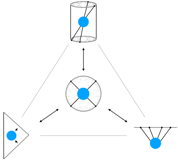
Figure 1: The Holographic Triangle: A cartoon representation of how perturbative observables at the conformal boundary in different maximally symmetric spaces can be recast in terms of boundary correlators in EAdS (centre). Top: $\Lambda<0$, bottom-right: $\Lambda>0$ and bottom-left: $\Lambda=0$.

The holographic principle is a very powerful idea which provides a framework to study quantum gravity observables living on the conformal boundary of space-time. This has been most successfully applied in the context of anti-de Sitter (AdS) space, where the AdS/CFT correspondence Maldacena:1997re ; Gubser:1998bc ; Witten:1998qj conjectures that quantum gravity observables on the boundary of AdS_d+1 space are equivalent to correlation functions of a (non-gravitational) Conformal Field Theory (CFT) in $d$-dimensional Minkowski space $\mathbb{M}^{d}$.

A key feature of AdS space is that its boundary lies at spatial infinity. The dual boundary theory is therefore a standard quantum mechanical system with a standard notion of locality and of time. This poses a key hurdle along the way to extend our understanding of holographic quantum gravity observables beyond the relative security of the AdS/CFT correspondence. Recent years have seen significant progress in the context of anti-de Sitter’s maximally symmetric (and more realistic) cousins Minkowski space and de Sitter (dS) space, which have come to be known as Celestial Holography Raclariu:2021zjz ; Pasterski:2021rjz ; McLoughlin:2022ljp ; Pasterski:2021raf and the Cosmological Bootstrap Baumann:2022jpr ; Benincasa:2022gtd , respectively. In contrast to AdS space, the conformal boundaries of Minkowski and dS space lie at null and past/future infinity, respectively, which obscures how the corresponding boundary correlation functions encode consistent bulk physics. Much of this progress has been driven by the discovery of connections with more familiar flat space S-matrices. In the context of celestial holography, celestial correlation functions have been defined as an integral transform of flat space scattering amplitudes deBoer:2003vf ; Cheung:2016iub ; Pasterski:2016qvg ; Pasterski:2017kqt . In the context of the Cosmological Bootstrap, a lot of mileage has been gained from the observation that the coefficient of the “total energy singularity” is the flat space scattering amplitude for the same process Maldacena:2011nz ; Raju:2012zr .

Another promising approach has been to draw connections with the well known perturbative computation of boundary correlators in AdS/CFT via Witten diagrams Cheung:2016iub ; Lam:2017ofc ; Sleight:2019hfp ; Sleight:2020obc ; DiPietro:2021sjt ; Sleight:2021plv ; Casali:2022fro ; PipolodeGioia:2022exe ; Iacobacci:2022yjo . It has been shown Sleight:2020obc ; Sleight:2021plv ; Iacobacci:2022yjo that both dS boundary correlators in the Bunch-Davies (Euclidean) vacuum and celestial correlation functions can be perturbatively recast as Witten diagrams in Euclidean AdS (EAdS). This approach, which places correlators on the boundary of EAdS at the centre, has been dubbed “the holographic triangle” (see figure 1). This is the idea that reformulating boundary correlators in AdS, Minkowski and dS as boundary correlators in EAdS could provide a way to place holography for $\Lambda<0$, $\Lambda=0$ and $\Lambda>0$ (i.e. for all $\Lambda$s) on a similar footing. How consistency criteria such as unitarity and causality are encoded in such EAdS boundary correlators depends on where the original theory is defined in the bulk (i.e Lorentzian AdS, Minkowski or de Sitter space).

In the context of celestial holography, it was recently noted that there seems to be a discrepancy between these two approaches to celestial correlators Iacobacci:2022yjo . In one case, celestial correlators are obtained from the corresponding S-matrix via an integral transform, while in the other celestial correlation functions are treated analogously to Witten diagrams. This discrepancy appears to arise from the fact that the relationship between celestial correlators and the S-matrix commutes divergent integrals forming part of the definition of conformal primary wavefunctions. In this work, we observe that the regularisation of the conformal primary wave functions defined in Pasterski:2016qvg ; Pasterski:2017kqt alters the definition of celestial correlators, which receive contributions from out of time order Minkowski correlators. In light of this, we propose a new definition for conformal primary wave functions as analytic functions that respect time-ordering in the bulk of Minkowski space, which are obtained by extrapolating one point of the Minkowski Feynman propagator $G_{F}$ to the celestial sphere. In practise, this is achieved by taking a Mellin transform with respect to the radial direction in the hyperbolic slicing of Minkowski space and the boundary limit in the hyperbolic directions:

$$G^{\text{flat}}_{\Delta}\left(X,Q\right)=\lim_{\hat{Y}\to Q}\int^{\infty}_{0}\frac{dt}{t}t^{\Delta}\,G_{F}\left(X,t\hat{Y}\right).$$ (1)

This definition treats conformal primary wave functions as analogous to bulk-to-boundary propagators in AdS space and is natural from an AdS/CFT perspective. We refer to these modified conformal primary wave functions $G^{\text{flat}}_{\Delta}$ as celestial bulk-to-boundary propagators. According to this definition, celestial correlators are given by a Mellin transform of time-ordered correlators in Minkowski space extrapolated to the boundary:

$$\left\langle\mathcal{O}_{\Delta_{1}}(Q_{1})\ldots\mathcal{O}_{\Delta_{n}}(Q_{n})\right\rangle=\prod_{i}\lim_{{\hat{Y}}_{i}\to Q_{i}}\,\int^{\infty}_{0}\frac{dt_{i}}{t_{i}}\,t_{i}^{\Delta_{i}}\left\langle\phi_{1}(t_{1}\hat{Y}_{1})\ldots\phi_{n}(t_{n}\hat{Y}_{n})\right\rangle.$$ (2)

This naturally extends the definition of boundary correlation functions commonly employed in (A)dS/CFT, which extrapolate bulk correlation functions to the conformal boundary.

Our proposed definition (2) of celestial correlators places bulk correlation functions at the centre of celestial holography. This has the advantage that it can be applied to theories in Minkowski space for which the S-matrix is not defined. An important example of such theories are Conformal Field Theories, which in Minkowski space are defined non-perturbatively at the level of correlation functions by Conformal Symmetry, Unitarity and a consistent operator product expansion. We note that the definition (2) opens up the possibility to study the properties of celestial correlation functions from their relatively well understood Minkowski CFT counterparts.

Coming back to the holographic triangle (figure 1), celestial correlators defined according to (2) can also be perturbatively re-cast as corresponding Witten diagrams in EAdS_d+1 along the same lines as Iacobacci:2022yjo . In this case, the relationship to EAdS Witten diagrams is more manifest owing to the fact that incoming and outgoing conformal primary modes are given by the same analytic function. In the hyperbolic slicing of Minkowksi space, the celestial bulk-to-boundary propagators (1) factorise into the corresponding bulk-to-boundary propagator in EAdS (suitably analytically continued) times a radial factor given by the kernel of the Konterovich-Lebedev transform. Contact diagram contributions to celestial correlation functions are therefore proportional to their EAdS Witten diagram counterparts upon integrating out the radial direction. This perturbative relationship between celestial correlators and EAdS Witten diagrams can then be extended beyond contact diagrams to processes involving particle exchanges by following the algorithm given in Iacobacci:2022yjo .

The plan of the paper is as follows: In section 2 we review the hyperbolic slicing of Minkowski space. In section 3 we revisit the definition of conformal primary wave functions and propose a new one given by celestial bulk-to-boundary propagators (1). In section 4 we explore celestial corelation functions (2) defined with respect to these new conformal primary wave functions, deriving the two-point function normalisation and considering $n$-point non-derivative contact diagrams in scalar theories. We show that celestial contact diagrams can be re-cast as corresponding contact Witten diagrams in EAdS_d+1 suitably analytically continued along the complexified null cone. In section 5 we highlight that the new definition (2) of celestial correlation functions applied to Minkowski CFTs in the bulk provides an opportunity to study celestial correlation functions from relatively well understood correlation functions in Minkowski CFTs. Various technical details are relegated to the appendices.

2 Hyperbolic slicing of Minkowski space

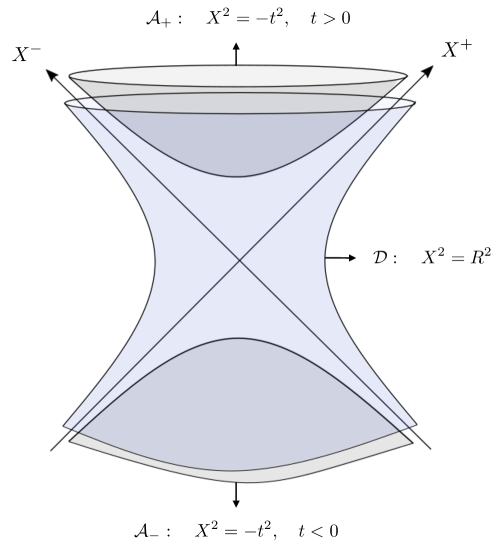
Figure 2: Hyperbolic foliation of Minkowski space with light-cone coordinates $X^{\pm}$.

In this work we consider $\left(d+2\right)$-dimensional Minkowski space $\mathbb{M}^{d+2}$ with Cartesian coordinates $X^{M}$, $M=0,\ldots,d+1$ and metric

$$ds^{2}=-\left(dX^{0}\right)^{2}+\left(dX^{1}\right)^{2}+\ldots+\left(dX^{d+1}\right)^{2}.$$ (3)

Following deBoer:2003vf , a radial foliation of $\mathbb{M}^{d+2}$ is naturally achieved by considering the following three regions:

$$\mathcal{D}: \quad X^{2}>0\,,$$ (4a)

$$\mathcal{A}_{+}: \quad X^{2}<0\,,\qquad X^{0}>0,$$ (4b)

$$\mathcal{A}_{-}: \quad X^{2}<0\,,\qquad X^{0}<0.$$ (4c)

Each region of these regions can be foliated with surfaces of constant curvature reflecting the $SO\left(d+1,1\right)$ symmetry. See figure 2. In regions $\mathcal{A}_{\pm}$ these are $\left(d+1\right)$-dimensional Euclidean anti-de Sitter spaces (EAdS_d+1) with constant radius $t$:

$$X^{2}=-t^{2}.$$ (5)

A natural set of coordinates for this foliation of ${\cal A}_{\pm}$ which is particularly well-suited for holography is given by Poincaré coordinates

$$\mathcal{A}_{+}: \qquad X^{M}=+\frac{t}{z}\left(\frac{1+z^{2}+\vec{x}^{2}}{2},\frac{1-z^{2}-\vec{x}^{2}}{2},\vec{x}\right), t >0,\quad z>0,$$ (6a)

$$\mathcal{A}_{-}: \qquad X^{M}=+\frac{t}{z}\left(\frac{1+z^{2}+\vec{x}^{2}}{2},\frac{1-z^{2}-\vec{x}^{2}}{2},\vec{x}\right), t <0,\quad z>0.$$ (6b)

For region ${\cal D}$ instead, the foliating surfaces are $\left(d+1\right)$-dimensional de Sitter space-times with radius $R$:

$$X^{2}=R^{2}.$$ (7)

It is convenient to cover each dS space with two Poincaré patches:

$$\mathcal{D}_{+}: \qquad X^{M}=\frac{R}{(-\eta)}\left(\frac{1-\eta^{2}+\vec{x}^{2}}{2},\frac{1+\eta^{2}-\vec{x}^{2}}{2},\vec{x}\right), R >0,\quad\eta<0$$ (8a)

$$\mathcal{D}_{-}: \qquad X^{M}=-\frac{R}{\eta}\left(\frac{1-\eta^{2}+\vec{x}^{2}}{2},\frac{1+\eta^{2}-\vec{x}^{2}}{2},\vec{x}\right), R >0,\quad\eta>0$$ (8b)

The two regions $\mathcal{D}_{\pm}$ of ${\cal D}$ correspond to expanding and contracting patches of the dS hypersurface (7) respectively:

$$\mathcal{D}_{+}: \quad X^{2}>0\,,\qquad X^{+}>0,$$ (9a)

$$\mathcal{D}_{-}: \quad X^{2}>0\,,\qquad X^{+}<0,$$ (9b)

where $X^{+}$ is the light cone coordinate $X^{+}=X^{0}+X^{1}$.

Conformal Boundary.

$\mathbb{M}^{d+2}$ has a conformal boundary at past and future null infinity, which is identified with the projective cone of light rays via

$$Q^{2}=0,\qquad Q\equiv\lambda Q,\qquad\lambda\in\mathbb{R}_{+}.$$ (10)

The past and future conformal boundaries are both $d$-dimensional spheres, which we shall denote by $S^{-}_{d}$ and $S^{+}_{d}$ respectively. To see this one introduces new projective coordinates

$$\xi_{1}=Q^{1}/Q^{0},\quad\xi_{2}=Q^{2}/Q^{0},\quad\ldots\quad,\quad\xi_{d+1}=Q^{d+1}/Q^{0},$$ (11)

so that

$$\xi^{2}_{1}+\ldots+\xi^{2}_{d+1}-1=0.$$ (12)

For the sphere $S^{-}_{d}$ we take $Q^{0}<0$ and for $S^{+}_{d}$ we take $Q^{0}>0$. These conformal boundaries of $\mathbb{M}^{d+2}$ are also conformal boundaries of each of its hyperbolic slices (5) and (7), which manifest from the fact that the slices asymptote to the lightcone (10). The region ${\cal A}_{+}\left({\cal A}_{-}\right)$ is foliated by the upper (lower) sheet of the hyperboloids (5) and have conformal boundary $S^{+}_{d}\left(S^{-}_{d}\right)$ at spatial infinity. In the parameterisations (6) the conformal boundary is reached by sending $z\to 0$ with boundary coordinates:

$$Q_{+} \sim\frac{t}{z}\,\left(\frac{1+x^{2}}{2},\frac{1-x^{2}}{2},\vec{x}\right), t>0,$$ with (13a)

$$Q_{-} \sim\frac{t}{z}\,\left(\frac{1+x^{2}}{2},\frac{1-x^{2}}{2},\vec{x}\right), t<0.$$ with (13b)

In region ${\cal D}$ the foliating surfaces (7) are de Sitter space-times, which each have a conformal boundary at future infinity $\left(S^{+}_{d}\right)$ and past infinity $\left(S^{-}_{d}\right)$. In the parameterisation (8) these are obtained in the limit $\eta\to 0$ with boundary coordinates:

$$Q_{+} \sim\frac{R}{(-\eta)}\left(\frac{1+x^{2}}{2},\frac{1-x^{2}}{2},\vec{x}\right), \eta<0,$$ with (14a)

$$Q_{-} \sim-\frac{R}{\eta}\left(\frac{1+x^{2}}{2},\frac{1-x^{2}}{2},\vec{x}\right), \eta>0.$$ with (14b)

Note that by working in complexified space one can analytically continue $Q_{+}$ to $Q_{-}$ by considering:

$$Q_{\theta}=e^{i\theta}\left(\frac{1+x^{2}}{2},\frac{1-x^{2}}{2},\vec{x}\right)\,.$$ (15)

Working in a complexified space-time will be useful when considering the analytic continuation in the next sections of this work.

3 Conformal Primary Wave Functions Revisited

In Pasterski:2016qvg ; Pasterski:2017kqt celestial correlation functions were defined as an integral transform of flat space scattering amplitudes by introducing the following conformal primary wave functions:

$$\phi^{\pm}_{\Delta}\left(X;Q\right)=\int_{H^{+}_{d+1}}\left[d{\hat{p}}\right]\frac{\Gamma(\Delta)}{(\pm im\hat{p}\cdot Q)^{\Delta}}\,e^{\pm im{\hat{p}}\cdot X},$$ (16)

where $H^{+}_{d+1}$ is the upper sheet of the $\left(d+1\right)$-dimensional unit hyperboloid ${\hat{p}}^{2}=-1$. It is instructive to note that these are obtained (up to normalisation) from the two-point Wightman function,

$$\mathcal{W}(X,Y)=\int d^{d+2}P\,\theta(P^{0})\delta(P^{2}+m^{2})\,e^{\pm iP\cdot(X-Y)},$$ (17)

by taking a Mellin transform of one of the points, say $Y=t\hat{Y}$, in the radial direction $t$ and extrapolating the remaining hyperbolic directions $\hat{Y}$ to the conformal boundary:

$$\phi^{\pm}_{\Delta}\left(X;Q\right)=\lim_{\hat{Y}\to Q_{\pm}}\int_{0}^{\infty}\frac{dt}{t}t^{\Delta}\,\mathcal{W}(X,t\hat{Y})\,.$$ (18)

In this work we shall refer to such a Mellin transform in the radial direction of $\mathbb{M}^{d+2}$ as a radial Mellin transform.

The defining integral (16) is divergent for generic $X$ and therefore must be defined by analytic continuation. This gives the following expression in terms of the Bessel-K function Pasterski:2016qvg ; Pasterski:2017kqt (see appendix B.1)

$$\phi^{\pm}(X,Q)=\Gamma(\Delta)\left(\frac{2\pi}{m}\right)^{\frac{d}{2}}\,\frac{(\sqrt{X^{2}\mp i\epsilon})^{\Delta-\frac{d}{2}}}{(-2X\cdot Q\mp i\epsilon)^{\Delta}}2{K}_{\Delta-\tfrac{d}{2}}(m\sqrt{X^{2}\mp i\epsilon})\,.$$ (19)

The latter definition however, appears to give rise to an inconsistency in the definition of the conformal primary wave function. This can be seen by taking the Fourier transform of the definition (19) (see Appendix B.2). Instead of the Wightman function from which we started, we obtain the off-shell (anti-)time ordered two-point function:

$$\tilde{\phi}^{\pm}(P,Q)=4\pi^{d+1}\left(\frac{m}{2}\right)^{\Delta-d}\frac{\pm i}{P^{2}+m^{2}\pm i\epsilon}\frac{\Gamma(\Delta)}{(\pm iQ\cdot P+\epsilon)^{\Delta}}\,.$$ (20)

Introducing the $i\epsilon$ prescription to regularise the integral (16) is therefore equivalent to selecting a time-ordering prescription for the 2pt function. It is the time-ordered Feynman propagator in the case of $\phi^{-}$ and the anti-time-ordered Feynman propagator in the case of $\phi^{+}$. Celestial correlation functions defined by the conformal primary wave functions (19) are therefore a radial Mellin transform of out-of-time-ordered correlation functions in $\mathbb{M}^{d+2}$ which are extrapolated to the conformal boundary in the hyperbolic directions.

In light of this, in this work we propose a natural definition of celestial correlation functions that manifestly respects the time-ordering of the bulk points in flat space. Such a definition would be given by conformal modes that are instead a radial Mellin transform of the Feynman propagator $G_{F}$:

$$G^{\text{flat}}_{\Delta}\left(X,Q\right)=\lim_{\hat{Y}\to Q}\int^{\infty}_{0}\frac{dt}{t}t^{\Delta}\,G_{F}\left(X,t\hat{Y}\right),$$ (21)

where incoming modes have $Q=Q_{-}\in S^{-}_{d}$ and outgoing modes have $Q=Q_{+}\in S^{+}_{d}$. Celestial correlation functions defined with respect to these new conformal modes $G^{\text{flat}}_{\Delta}$ are then a radial Mellin transform of time-ordered correlation functions in $\mathbb{M}^{d+2}$ which are extrapolated to the conformal boundary in the hyperbolic directions. This modified prescription would naturally generalise the definition of boundary correlators commonly employed in the context of (A)dS/CFT, which extrapolate bulk correlation functions to the conformal boundary. This is explored in more detail in the next section.

We refer to the new proposed conformal mode $G^{\text{flat}}_{\Delta}\left(X,Q\right)$ as the celestial bulk-to-boundary propagator. In appendix C we show that the celestial bulk-to-boundary propagator can be expressed explicitly in the following form

$$G^{\text{flat}}_{\Delta}(X,Q) =c_{\Delta}^{\text{flat-AdS}}G^{\text{AdS}}_{\Delta}(\hat{X}_{\epsilon},Q)\,\mathcal{K}^{(m)}_{i\left(\frac{d}{2}-\Delta_{i}\right)}\left(\sqrt{X^{2}+i\epsilon}\right)\,,$$ (22)

in terms of the the kernel $\mathcal{K}^{(m)}_{i\left(\frac{d}{2}-\Delta_{i}\right)}$ of the Konterovich-Lebedev transform (see Appendix A) and the corresponding (analytically continued) EAdS_d+1 bulk-to-boundary propagator:

$$G^{\text{AdS}}_{\Delta}(\hat{X}_{\epsilon},Q)=C^{\text{AdS}}_{\Delta}\frac{\left(\sqrt{X^{2}+i\epsilon}\right)^{\Delta}}{(-2X\cdot Q+i\epsilon)^{\Delta}}\,,$$ (23)

with

$$C^{\text{AdS}}_{\Delta} =\frac{\Gamma(\Delta)}{2\pi^{d/2}\Gamma\left(\Delta-\frac{d}{2}+1\right)}\,.$$ (24)

The coefficient

$$c_{\Delta}^{\text{flat-AdS}}=\frac{C^{\text{flat}}_{\Delta}}{C^{\text{AdS}}_{\Delta}}=\frac{1}{2}\,\csc(\pi(\tfrac{d}{2}-\Delta)),$$ (25)

can be thought of as accounting for the difference in two-point function normalisation between AdS (24) and flat (29) (which is computed in section 4.1).

Let us make a few comments:

• The starting point in the definition of celestial bulk-to-boundary (21) is a well-defined analytic function dictated by the $i\epsilon$ prescription of the Feynman propagator. This is to be contrasted with the definition (16) of conformal primary wave functions commonly used in the literature, where the starting point is a divergent integral.

• The definition (16) has been used to define celestial correlators as an integral transform of flat space scattering amplitudes. This definition of celestial correlators commutes the divergent integral (16) with the integral over Minkowski space. As noted in Iacobacci:2022yjo , this seemed to lead to a discrepancy when one instead regulates the conformal primary wave function according to (19) and leaves evaluating the integral over Minkowski space to the end i.e. treating celestial correlators analogously to Witten diagrams in AdS. The above results clarify that the regularisation (19) modifies the definition of the celestial correlator and appears to explain the discrepancy noted in Iacobacci:2022yjo . The action of commuting the divergent integral (16) with the integral over Minkowski space to relate celestial correlators to flat space scattering amplitudes seems to throw away off-shell contributions.

• For the modified definition (21) of conformal primary wave function, incoming and outgoing modes are given by the same analytic function (22) with $Q=Q_{-}\in S^{-}_{d}$ for incoming modes and $Q=Q_{+}\in S^{+}_{d}$ for outgoing modes. In the hyperbolic slicing this function is factorised into the (analytically continued) AdS bulk-to-boundary propagator times a radial dependence given by the kernel of the Konterovich-Lebedev transform, which makes manifest that celestial correlators can be (at least perturbatively) re-cast as (suitably analytically continued) AdS Witten diagrams. This is discussed in more detail in the next section.

• The Feynman propagator is recovered by the inverse Mellin transform:

  $$G_{F}(X,tQ)=\int_{\frac{d}{2}-i\infty}^{\frac{d}{2}+i\infty}\frac{d\Delta}{2\pi i}\,c_{\Delta}^{\text{flat-AdS}}G^{\text{AdS}}_{\Delta}(\hat{X}_{\epsilon},Q)\,\mathcal{K}^{(m)}_{i\left(\frac{d}{2}-\Delta_{i}\right)}\left(\sqrt{X^{2}+i\epsilon}\right)\,t^{-\Delta}\,,$$ (26)

  which is equivalent (as expected) to the inverse Konterovich-Lebedev transform (see appendix A).

4 Celestial Correlators Revisited

In this section we re-visit the definition of celestial correlation functions in the light of the newly proposed definition (21) of conformal primary wave functions. According to this modified definition, celestial correlation functions are related to time-ordered correlation functions in Minkowski space by taking the radial Mellin-transform of each external point and extrapolating the remaining hyperbolic directions to the conformal boundary:

$$\left\langle\mathcal{O}_{\Delta_{1}}(Q_{1})\ldots\mathcal{O}_{\Delta_{n}}(Q_{n})\right\rangle=\prod_{i}\lim_{{\hat{Y}}_{i}\to Q_{i}}\,\int^{\infty}_{0}\frac{dt_{i}}{t_{i}}\,t_{i}^{\Delta_{i}}\left\langle\phi_{1}(t_{1}\hat{Y}_{1})\ldots\phi_{n}(t_{n}\hat{Y}_{n})\right\rangle.$$ (27)

This definition naturally extends the definition of boundary correlation functions commonly employed in (A)dS/CFT, which extrapolate bulk correlation functions to the conformal boundary. The difference is that in Minkowski space one must first perform a radial Mellin transform which integrates out the radial direction, after which one extrapolates to the conformal boundary as one does in (A)dS/CFT.

In the following sections we evaluate the above-defined celestial correlators in some examples for massive scalar field theories. We furthermore show that they can be perturbatively recast in terms of corresponding AdS Witten diagrams suitably analytically continued along the complex light-cone.

4.1 Two-point function normalisation

Let us first determine the normalisation of the celestial two-point function. This is obtained from the celestial bulk-to-boundary propagator (21) by taking the radial Mellin transform of the remaining bulk point and the boundary limit in the hyperbolic directions:

$$\langle\mathcal{O}_{\Delta_{1}}\left(Q_{1}\right)\mathcal{O}_{\Delta_{2}}\left(Q_{2}\right)\rangle =\lim_{{\hat{X}}\to Q_{2}}\int_{0}^{\infty}\frac{dt}{t}\,t^{\Delta_{2}}G^{\text{flat}}_{\Delta_{1}}(t{\hat{X}},Q_{1})$$ (28)

$$=\left(\frac{m}{2}\right)^{d-2\Delta_{1}}\,\frac{C^{\text{flat}}_{\Delta_{1}}}{(-2Q_{1}\cdot Q_{2}+i\epsilon)^{\Delta_{1}}}(2\pi)\delta(i(\Delta_{1}-\Delta_{2}))\,,$$

with normalisation

$$C^{\text{flat}}_{\Delta}=\frac{1}{2\pi^{\frac{d+2}{2}}}\,\Gamma(\Delta)\Gamma(\Delta-\tfrac{d}{2}).$$ (29)

Note that the two point function is non-vanishing in the case that one operator is on the past boundary and the other on the future boundary. Such two point functions differ by phase factors which are encoded in the $i\epsilon$ prescription in eq. (28):

$$\left\langle\mathcal{O}_{\Delta_{1}}^{i}(Q_{1})\mathcal{O}_{\Delta_{2}}^{j}(Q_{2})\right\rangle\\ =\left(\frac{m}{2}\right)^{d-2\Delta_{1}}\begin{pmatrix}1&e^{-i\pi\Delta_{1}}\\ e^{-i\pi\Delta_{1}}&1\end{pmatrix}\frac{C^{\text{flat}}_{\Delta_{1}}}{|-2Q_{1}\cdot Q_{2}|^{\Delta_{1}}}\,(2\pi)\delta(i(\Delta_{1}-\Delta_{2}))\,.$$ (30)

This is diagonalised by the following orthogonal operators:

$$\mathcal{O}^{>}_{\Delta} =\frac{e^{i\frac{\pi}{4}(\Delta-1)}}{2}\left(\mathcal{O}_{\Delta}^{-}-\mathcal{O}_{\Delta}^{+}\right),$$ (31a)

$$\mathcal{O}^{<}_{\Delta} =\frac{e^{i\frac{\pi}{4}\Delta}}{2}\left(\mathcal{O}_{\Delta}^{-}+\mathcal{O}_{\Delta}^{+}\right),$$ (31b)

with two-point functions:

$$\left\langle\mathcal{O}_{\Delta_{1}}^{>}(Q_{1})\mathcal{O}_{\Delta_{2}}^{>}(Q_{2})\right\rangle =\left(\frac{m}{2}\right)^{d-2\Delta_{1}}\sin\left(\tfrac{\pi}{2}\Delta_{1}\right)\frac{C^{\text{flat}}_{\Delta_{1}}}{|-2Q_{1}\cdot Q_{2}|^{\Delta_{1}}}\,(2\pi)\delta(i(\Delta_{1}-\Delta_{2})),$$ (32a)

$$\left\langle\mathcal{O}_{\Delta_{1}}^{<}(Q_{1})\mathcal{O}_{\Delta_{2}}^{<}(Q_{2})\right\rangle =\left(\frac{m}{2}\right)^{d-2\Delta_{1}}\cos\left(\tfrac{\pi}{2}\Delta_{1}\right)\frac{C^{\text{flat}}_{\Delta_{1}}}{|-2Q_{1}\cdot Q_{2}|^{\Delta_{1}}}\,(2\pi)\delta(i(\Delta_{1}-\Delta_{2})).$$ (32b)

4.2 Contact diagrams

In this section we consider consider contact diagrams in a theory of scalar fields $\phi_{i}$, $i=1,\ldots,n$, which interact through the vertex

$${\cal V}\left(X\right)=g\phi_{1}\left(X\right)\ldots\phi_{n}\left(X\right).$$ (33)

At linear order in the coupling $g$, the corresponding $n$-point celestial correlator is given by

$$\left\langle\mathcal{O}_{1}(Q_{1})\ldots\mathcal{O}_{n}(Q_{n})\right\rangle=-ig\int d^{d+2}X\,G_{\Delta_{1}}^{\text{flat}}(X,Q_{1})\cdots G_{\Delta_{n}}^{\text{flat}}(X,Q_{n})\,.$$ (34)

Recall that the celestial bulk-to-boundary propagator factorise (22) into the corresponding (analytically continued) EAdS bulk-to-boundary propagator times the kernel of the Konterovich-Lebedev transform encoding the radial direction. This makes manifest that celestial contact diagrams are proportional to their corresponding Witten diagrams in EAdS upon integrating out the radial direction. In appendix E, using the explicit expression (22) for the Celestial bulk-to-boundary propagators, it is shown how the integral over $X\in\mathbb{M}^{d+2}$ in two different ways: 1. In Cartesian coordinates. 2. In the hyperbolic slicing of $\mathbb{M}^{d+2}$. Both ways give the same factorised result:

$$\left\langle\mathcal{O}_{1}(Q_{1})\ldots\mathcal{O}_{n}(Q_{n})\right\rangle=\sin\left(\tfrac{\pi}{2}(\Delta_{1}+\ldots+\Delta_{n}-d)\right)\left(\prod_{i}c^{\text{flat-AdS}}_{\Delta_{i}}\right)\\ \times R_{\Delta_{1}\ldots\Delta_{n}}\left(m_{1},\ldots,m_{n}\right)D_{\Delta_{1}\ldots\Delta_{n}}(Q_{1},\ldots,Q_{n}),$$ (35)

where $D_{\Delta_{1}\dots\Delta_{n}}(Q_{1},\ldots,Q_{n})$ is the familiar EAdS D-function DHoker:1999kzh , which here is defined over the complexified light-cone $Q_{i}^{2}=0$ via the $i\epsilon$ prescription of the celestial bulk-to-boundary propagator (see appendix D). The coefficient $R_{\Delta_{1}\dots\Delta_{n}}\left(m_{1},\ldots,m_{n}\right)$ instead arises from the integral over the radial direction and is naturally given by the following Mellin-Barnes integral (see appendix E.2):

$$R_{\Delta_{1}\dots\Delta_{n}}\left(m_{1},\ldots,m_{n}\right)=\int[ds_{i}]_{n}(2\pi i)\delta\left(-\frac{d+2}{2}+\sum_{j}\left(s_{j}+\tfrac{d}{4}\right)\right)\prod_{i}\widetilde{{\cal K}}^{\left(m_{i}\right)}_{i\left(\frac{d}{2}-\Delta_{i}\right)}(s_{i})\,,$$ (36)

where $\widetilde{{\cal K}}^{\left(m_{i}\right)}_{i\left(\frac{d}{2}-\Delta_{i}\right)}(s_{i})$ is the Mellin transform of kernel $\mathcal{K}^{(m)}_{i\left(\frac{d}{2}-\Delta_{i}\right)}$ of the Konterovich-Lebedev transform (see Appendix A). It is interesting to note the similarity between the (36) for the radial integral and the corresponding contact Witten diagram in momentum space (cf. equation (3.19) of Sleight:2021plv ).

Let us make a few comments:

• In a previous work Iacobacci:2022yjo we instead employed the conventional definition (19) of conformal primary wave functions to show that celestial correlators can be perturbatively re-cast as AdS Witten diagrams. In the above we have shown that such a relationship with AdS Witten diagrams also holds for their modified definition (21), though there are some key differences. In particular, when using the conventional definition (19), the contribution (36) from the radial direction contains folded singularities in the mass $m_{i}$ owing to the fact that, according to the conventional definition (19), incoming and outgoing conformal primary wave functions have different $i\epsilon$ prescriptions. See equation (4.24) of Iacobacci:2022yjo . Using the modified prescription (21), where incoming and outgoing modes have the same $i\epsilon$ prescription, the entire radial contribution (36) now resembles a momentum space contact Witten diagram in EAdS where the masses $m_{i}$ play the role of the modulus of the boundary momentum and the Konterovich-Lebedev kernels are proportional to the momentum space EAdS bulk-to-boundary propagators. It would be interesting to understand whether there is any significance behind these similarities with momentum space EAdS Witten diagrams in the radial contribution.

• The overall sinusoidal factor

  $$\sin\left(\tfrac{\pi}{2}(\Delta_{1}+\ldots+\Delta_{n}-d)\right),$$ (37)

  arises from combining the contributions (appendix E.2) from the regions ${\cal A}_{\pm}$ and ${\cal D}_{\pm}$ in the hyperbolic slicing of $\mathbb{M}^{d+2}$, which each differ by a phase. This is reminiscent of a similar result for contact diagram contributions to boundary correlation functions in dS space, which are related to their corresponding EAdS contact Witten diagrams by multiplying the latter by a sinusoidal factor depending on $\Delta_{i}$, $n$ and $d$. In that case the sinusoidal factor arose from combining the contributions to the dS contact diagram from each branch of the in-in contour Sleight:2019mgd ; Sleight:2019hfp ; Sleight:2020obc ; Sleight:2021plv , which have an equal and opposite phase. In the present case the regions ${\cal A}_{\pm}$ and ${\cal D}_{\pm}$ are the analogues are the $\pm$ branches of the in-in contour. The factor (37) suggests that the celestial contact diagrams are vanishing for certain values of $\Delta_{i}$, $n$ and $d$.

• We have shown that celestial contact diagrams are proportional to the corresponding contact Witten diagram in EAdS_d+1 (appropriately analytically continued on the complexified null cone). In other words

  $$\left\langle\mathcal{O}_{1}(Q_{1})\ldots\mathcal{O}_{n}(Q_{n})\right\rangle=c_{\Delta_{1}\ldots\Delta_{n}}D_{\Delta_{1}\ldots\Delta_{n}}(Q_{1},\ldots,Q_{n}),$$ (38)

  where $c_{\Delta_{1}\ldots\Delta_{n}}$ can be thought of as the ratio

  $$c_{\Delta_{1}\ldots\Delta_{n}}=\frac{\lambda^{\text{flat}}_{\Delta_{1}\ldots\Delta_{n}}}{\lambda^{\text{AdS}}_{\Delta_{1}\ldots\Delta_{n}}},$$ (39)

  of the coefficient $\lambda^{\text{AdS}}_{\Delta_{1}\ldots\Delta_{n}}$ of the contact Witten diagram and $\lambda^{\text{flat}}_{\Delta_{1}\ldots\Delta_{n}}$ the coefficient of the celestial contact diagram. As noted in Iacobacci:2022yjo , as a result of on-shell factorisation this perturbative relationship between celestial correlators and EAdS Witten diagrams extends beyond contact diagrams to processes involving particle exchanges. By following the algorithm provided in Iacobacci:2022yjo , any given perturbative celestial correlator can be recast in terms of corresponding EAdS_d+1 Witten diagrams.

3pt contact diagrams. A simple and instructive example is the case of 3pt functions, where (see appendix D):

$$D_{\Delta_{1}\Delta_{2}\Delta_{3}}(Q_{1},Q_{2},Q_{3})\\ =\frac{\lambda^{\text{AdS}}_{\Delta_{1}\Delta_{2}\Delta_{3}}}{(-2Q_{1}\cdot Q_{2}+i\epsilon)^{\frac{\Delta_{1}+\Delta_{2}-\Delta_{3}}{2}}(-2Q_{2}\cdot Q_{3}+i\epsilon)^{\frac{\Delta_{2}+\Delta_{3}-\Delta_{1}}{2}}(-2Q_{3}\cdot Q_{1}+i\epsilon)^{\frac{\Delta_{3}+\Delta_{1}-\Delta_{2}}{2}}}\,.$$ (40)

Note that the $i\epsilon$ prescription allows to define the above correlator on the complexified light-cone, thus allowing to seamlessly analytically continue from $Q_{+}$ to $Q_{-}$ and vice-versa. The coefficient is proportional to the standard 3pt Witten-diagram coefficient (see e.g. equation (131) of Costa:2014kfa ) and is given by:

$$\lambda^{\text{AdS}}_{\Delta_{1},\Delta_{2},\Delta_{3}}=-g\frac{\Gamma\left(\tfrac{\Delta_{1}+\Delta_{2}+\Delta_{3}-d}{2}\right)\Gamma\left(\tfrac{\Delta_{1}+\Delta_{2}-\Delta_{3}}{2}\right)\Gamma\left(\tfrac{\Delta_{2}+\Delta_{3}-\Delta_{1}}{2}\right)\Gamma\left(\tfrac{\Delta_{3}+\Delta_{1}-\Delta_{2}}{2}\right)}{16\pi^{d}\,\Gamma\left(\Delta_{1}-\tfrac{d}{2}+1\right)\Gamma\left(\Delta_{2}-\tfrac{d}{2}+1\right)\Gamma\left(\Delta_{3}-\tfrac{d}{2}+1\right)}.$$ (41)

By simplifying the $i\epsilon$ prescription one obtains:

$$D^{\pm\pm\pm}_{\Delta_{1}\Delta_{2}\Delta_{3}}(Q_{1},Q_{2},Q_{3}) =\frac{\lambda^{\text{AdS}}_{\Delta_{1},\Delta_{2},\Delta_{3}}}{|-2Q_{1}\cdot Q_{2}|^{\frac{\Delta_{1}+\Delta_{2}-\Delta_{3}}{2}}|-2Q_{2}\cdot Q_{3}|^{\frac{\Delta_{2}+\Delta_{3}-\Delta_{1}}{2}}|-2Q_{3}\cdot Q_{1}|^{\frac{\Delta_{3}+\Delta_{1}-\Delta_{2}}{2}}}$$

$$\hskip 14.22636pt+\text{contact}\,,$$ (42a)

$$D^{\pm\pm\mp}_{\Delta_{1}\Delta_{2}\Delta_{3}}(Q_{1},Q_{2},Q_{3}) =\frac{\lambda^{\text{AdS}}_{\Delta_{1},\Delta_{2},\Delta_{3}}e^{-i\pi\Delta_{3}}}{|-2Q_{1}\cdot Q_{2}|^{\frac{\Delta_{1}+\Delta_{2}-\Delta_{3}}{2}}|-2Q_{2}\cdot Q_{3}|^{\frac{\Delta_{2}+\Delta_{3}-\Delta_{1}}{2}}|-2Q_{3}\cdot Q_{1}|^{\frac{\Delta_{3}+\Delta_{1}-\Delta_{2}}{2}}}$$

$$\hskip 14.22636pt+\text{contact}\,,$$ (42b)

$$D^{\pm\mp\pm}_{\Delta_{1}\Delta_{2}\Delta_{3}}(Q_{1},Q_{2},Q_{3}) =\frac{\lambda^{\text{AdS}}_{\Delta_{1},\Delta_{2},\Delta_{3}}e^{-i\pi\Delta_{2}}}{|-2Q_{1}\cdot Q_{2}|^{\frac{\Delta_{1}+\Delta_{2}-\Delta_{3}}{2}}|-2Q_{2}\cdot Q_{3}|^{\frac{\Delta_{2}+\Delta_{3}-\Delta_{1}}{2}}|-2Q_{3}\cdot Q_{1}|^{\frac{\Delta_{3}+\Delta_{1}-\Delta_{2}}{2}}}$$

$$\hskip 14.22636pt+\text{contact}\,$$ (42c)

$$D^{\mp\pm\pm}_{\Delta_{1}\Delta_{2}\Delta_{3}}(Q_{1},Q_{2},Q_{3}) =\frac{\lambda^{\text{AdS}}_{\Delta_{1},\Delta_{2},\Delta_{3}}e^{-i\pi\Delta_{1}}}{|-2Q_{1}\cdot Q_{2}|^{\frac{\Delta_{1}+\Delta_{2}-\Delta_{3}}{2}}|-2Q_{2}\cdot Q_{3}|^{\frac{\Delta_{2}+\Delta_{3}-\Delta_{1}}{2}}|-2Q_{3}\cdot Q_{1}|^{\frac{\Delta_{3}+\Delta_{1}-\Delta_{2}}{2}}}$$

$$\hskip 14.22636pt+\text{contact}\,$$ (42d)

where $\pm$ refers to $Q_{i}\in S^{\pm}_{d}$ and where the contact terms are proportional to distributional pieces in the $Q_{i}$ as $\epsilon\to 0$. Similar expressions can be recovered for higher-point functions.

5 Celestial correlators for Minkowski CFTs

In this work we have proposed a new definition of celestial correlation functions as the Mellin transform of correlation functions in Minkowski space extrapolated to the conformal boundary:

$$\left\langle\mathcal{O}_{\Delta_{1}}(Q_{1})\ldots\mathcal{O}_{\Delta_{n}}(Q_{n})\right\rangle=\prod_{i}\lim_{{\hat{Y}}_{i}\to Q_{i}}\,\int^{\infty}_{0}\frac{dt_{i}}{t_{i}}\,t_{i}^{\Delta_{i}}\left\langle\phi_{1}(t_{1}\hat{Y}_{1})\ldots\phi_{n}(t_{n}\hat{Y}_{n})\right\rangle.$$ (43)

This definition allows to define celestial correlation functions for any theory in Minkowski space, even in cases where the S-matrix does not exist.

CFTs in Minkowski space are important examples of theories where the standard notion of an S-matrix is ill-defined. Despite this, Minkowski CFTs are defined non-perturbatively by conformal symmetry, unitarity and a consistent operator product expansion, which are the three main pillars of the conformal bootstrap programme Simmons-Duffin:2016gjk ; Poland:2018epd . This is to be contrasted with our understanding of the properties of celestial correlation functions and how they encode consistent Minkowski bulk physics. Taking the bulk Minkowski theory to be a CFT, the definition (43) provides an opportunity to study the properties of celestial correlation functions from their relatively well understood Minkowski CFT counterparts!

Three and four-point conformal correlation functions of quasi-primary fields $\phi_{{\bar{\Delta}}_{i}}$ in $\mathbb{M}^{d+2}$ are constrained by conformal symmetry to take the following form Polyakov:1970xd

$$\left\langle\phi_{{\bar{\Delta}}_{1}}(X_{1})\phi_{{\bar{\Delta}}_{2}}(X_{2})\phi_{{\bar{\Delta}}_{3}}(X_{3})\right\rangle =\frac{f_{{\bar{\Delta}}_{1},{\bar{\Delta}}_{2},{\bar{\Delta}}_{3}}}{(X_{12}^{2})^{\frac{{\bar{\Delta}}_{1}+{\bar{\Delta}}_{2}-{\bar{\Delta}}_{3}}{2}}(X_{23}^{2})^{\frac{{\bar{\Delta}}_{2}+{\bar{\Delta}}_{3}-{\bar{\Delta}}_{1}}{2}}(X_{31}^{2})^{\frac{{\bar{\Delta}}_{3}+{\bar{\Delta}}_{1}-{\bar{\Delta}}_{2}}{2}}}\,,$$ (44a)

$$\left\langle\phi_{{\bar{\Delta}}_{1}}(X_{1})\phi_{{\bar{\Delta}}_{2}}(X_{2})\phi_{{\bar{\Delta}}_{3}}(X_{3})\phi_{{\bar{\Delta}}_{4}}(X_{4})\right\rangle =\frac{1}{(X_{12}^{2})^{\frac{{\bar{\Delta}}_{1}+{\bar{\Delta}}_{2}}{2}}(X_{34}^{2})^{\frac{{\bar{\Delta}}_{3}+{\bar{\Delta}}_{4}}{2}}}\left(\frac{X_{24}^{2}}{X_{14}^{2}}\right)^{\frac{{\bar{\Delta}}_{1}-{\bar{\Delta}}_{2}}{2}}\left(\frac{X_{14}^{2}}{X_{13}^{2}}\right)^{\frac{{\bar{\Delta}}_{3}-{\bar{\Delta}}_{4}}{2}}\,f(u,v),$$ (44b)

where $f_{{\bar{\Delta}}_{1},{\bar{\Delta}}_{2},{\bar{\Delta}}_{3}}$ is a constant and $f(u,v)$ a function of the usual conformal invariant cross ratios $u$ and $v$. We use the notation $X^{2}_{ij}=\left(X_{i}-X_{j}\right)^{2}$. To plug these into the definition (43) of celestial correlation functions we take the light-cone limit $X_{i}\to t_{i}Q_{i}$. In this limit the we have $X^{2}_{ij}\to-2t_{i}t_{j}Q_{i}\cdot Q_{j}$, which are homogeneous in the $t_{i}$ and simplifies significantly the the Mellin transform (43), which reduce to the integrals

$$\int_{0}^{\infty}\frac{dt_{i}}{t_{i}}\,t_{i}^{\Delta_{i}-{\bar{\Delta}}_{i}}=2\pi\delta(i(\Delta_{i}-{\bar{\Delta}}_{i}))\,.$$ (45)

The celestial correlation functions corresponding to the Minkowski conformal three- and four-point functions (44) are therefore

$$\left\langle O_{\Delta_{1}}(Q_{1})O_{\Delta_{2}}(Q_{2})O_{\Delta_{3}}(Q_{3})\right\rangle\\ =\frac{f_{\Delta_{1},\Delta_{2},\Delta_{3}}\prod\limits^{3}_{i=1}2\pi\delta(i(\Delta_{i}-{\bar{\Delta}}_{i}))}{(X_{12}^{2})^{\frac{\Delta_{1}+\Delta_{2}-\Delta_{3}}{2}}(X_{23}^{2})^{\frac{\Delta_{2}+\Delta_{3}-\Delta_{1}}{2}}(X_{31}^{2})^{\frac{\Delta_{3}+\Delta_{1}-\Delta_{2}}{2}}}\Bigg{|}_{X_{ij}^{2}\to-2Q_{i}\cdot Q_{j}+i\epsilon}\,,$$ (46)

$$\left\langle O_{\Delta_{1}}(Q_{1})O_{\Delta_{2}}(Q_{2})O_{\Delta_{3}}(Q_{3})O_{\Delta_{4}}(Q_{4})\right\rangle =\frac{\prod\limits^{4}_{i=1}2\pi\delta(i(\Delta_{i}-{\bar{\Delta}}_{i}))}{(X_{12}^{2})^{\frac{\Delta_{1}+\Delta_{2}}{2}}(X_{34}^{2})^{\frac{\Delta_{3}+\Delta_{4}}{2}}}$$ (47)

$$\times\left(\frac{X_{24}^{2}}{X_{14}^{2}}\right)^{\frac{\Delta_{1}-\Delta_{2}}{2}}\left(\frac{X_{14}^{2}}{X_{13}^{2}}\right)^{\frac{\Delta_{3}-\Delta_{4}}{2}}\,f(u,v)\Bigg{|}_{X_{ij}^{2}\to-2Q_{i}\cdot Q_{j}+i\epsilon}\,,$$

where $u$ and $v$ are now the cross-ratios in $d$-dimensions. These are Euclidean conformal correlators in $d$ dimensions and the $i\epsilon$ prescription inherited from the Bulk Minkowski CFT allows to distinguish in and out operators depending on whether $Q_{i}\in S_{d}^{\pm}$.

Let us consider a simple concrete example. The mean field theory correlation function of an operator $\phi$ with scaling dimension $\Delta$ is given by

$$\left\langle\phi(Q_{1})\phi(Q_{2})\phi(Q_{3})\phi(Q_{4})\right\rangle=\frac{1}{(X_{12}^{2}X_{34}^{2})^{\Delta}}\left(1+u^{\Delta}+\left(\frac{u}{v}\right)^{\Delta}\right)\,.$$ (48)

The corresponding celestial correlation function is

$$\left\langle O_{\Delta_{1}}^{+}(Q_{1})O_{\Delta_{2}}^{+}(Q_{2})O_{\Delta_{3}}^{-}(Q_{3})O_{\Delta_{4}}^{-}(Q_{4})\right\rangle\\ =\frac{\prod\limits^{4}_{i=1}2\pi\delta(i(\Delta_{i}-\Delta))}{(y_{12}^{2}y_{34}^{2})^{\Delta}}\left(1+e^{-2\pi i\Delta}u^{\Delta}+e^{-2\pi i\Delta}\left(\frac{u}{v}\right)^{\Delta}\right)\,,$$ (49)

where the $y_{i}$ are $d$-dimensional Euclidean vectors and we took $Q_{1,2}\in S^{+}_{d}$ and $Q_{3,4}\in S^{-}_{d}$. The phase factors $e^{-2\pi i\Delta}$ originate from the bulk $i\epsilon$ prescription and thus encode bulk Minkowski causality. These examples could therefore be useful toy models to gain a better understanding of celestial CFTs and how they encode bulk unitarity and causality. We leave a detailed analysis of the properties of the above celestial correlators for the future!

6 Conclusions

We conclude with some future directions:

• While our prescription for celestial correlation functions holds both for massive and massless particles, it would be desirable to study in the massless case in more detail. In this case, the conformal boundary can be reached on-shell, thus suggesting that there should be a relation between our prescription and the $S$-matrix for massless particles. It would be very interesting to see if the two prescriptions for celestial correlators can be related and how the S-matrix is embedded within celestial correlators defined with our prescription.

• Independently of the above point, we note that it is possible to put external legs on-shell by considering the discontinuity of the Feynman propagator:

  $$\text{Disc}_{P^{2}}\left[\frac{1}{P^{2}+m^{2}-i\epsilon}\right]=\Im\left[\frac{1}{P^{2}+m^{2}-i\epsilon}\right]=(2\pi i)\delta(P^{2}+m^{2})\,.$$ (50)

  Taking the Mellin transform of the above equation one thus end up with a consistent regularisation for the Mellin transform of the on-shell condition:

  $$\text{disc}\left[G_{\Delta}^{\text{flat}}(X,Q)\right]=\Im\left[\lim_{\hat{Y}\to Q}\int_{0}^{\infty}\frac{dt}{t}\,t^{\Delta}\,G_{F}(X,t\hat{Y})\right]\,.$$ (51)

  At the level of celestial correlation functions this is equivalent to taking the discontinuity with respect to all external legs:

  $$\left\langle\mathcal{O}_{\Delta_{1}}(Q_{1})\ldots\mathcal{O}_{\Delta_{n}}(Q_{n})\right\rangle\Big{|}_{\text{on-shell}}\\ =\prod_{i}\Im_{i}\left[\prod_{i}\lim_{{\hat{Y}}_{i}\to Q_{i}}\,\int^{\infty}_{0}\frac{dt_{i}}{t_{i}}\,t_{i}^{\Delta_{i}}\left\langle\phi_{1}(t_{1}\hat{Y}_{1})\ldots\phi_{n}(t_{n}\hat{Y}_{n})\right\rangle\right],$$ (52)

  which is related to the S-matrix via the LSZ formula. This might elucidate the relation between the prescription proposed in this work and the S-matrix.

• An advantage of this modified definition of celestial correlators is that it applies to theories which do not have an S-matrix. An important example of such theories are Minkowski CFTs. A more detailed study of our prescription in the case that the bulk theory is a Minkowski CFT would be relevant to understand non-perturbative properties of the exotic Euclidean CFTs arising at the boundary of Minkowski space, such as unitarity, causality and analyticity and how they are encoded. From the simple examples we have considered it is already apparent that the Celestial correlators dual to Minkowski CFTs are distributions and it would be interesting to clarify their analyticity properties more generally.

• Note that, taking $Q_{1,2}\in S^{+}_{d}$ and $Q_{3,4}\in S^{-}_{d}$ the definition (2) of celestial four-point functions is such that the corresponding singularities corresponds to the Regge limit of the bulk Minkowski correlator. It would be interesting to clarify the interplay between bulk Minkowski correlator, their Regge limit and Celestial correlators.

• The fact that celestial correlation functions can be perturbatively recast as Witten diagrams in EAdS implies that they have the same analytic structure and in particular admit a conformal partial wave decomposition. Assuming that this continues to hold at the non-perturbative level, it was noted in Iacobacci:2022yjo that unitarity implies a non-perturbative positivity constraint on the spectral density of celestial four-point functions - generalising the same observation Hogervorst:2021uvp ; DiPietro:2021sjt for dS boundary correlators to any unitary Euclidean CFT. It would be interesting use this to derive non-perturbative constraints on bulk Minkowski physics.

• Our prescription naturally extends to the case of spinning fields. While the extension to massive spinning fields looks straightforward, in the massless case it will be important to study BMS symmetries for the celestial correlators so defined, derive the corresponding Ward identities and identify soft degrees of freedom at the boundary e.g. along the lines of Donnay:2018neh ; Donnay:2020guq ; Donnay:2022sdg .

Appendix A The Konterovich-Lebedev transform

A complete orthogonal basis for elements of $L^{2}\left(\mathbb{R}^{+},dRR^{d-1}\right)$ are given by

$$\mathcal{K}^{(m)}_{\alpha}(R)=\left\langle R|\tilde{K}^{(m)}_{\alpha}\right\rangle=\left(\frac{m}{2}\right)^{-i\alpha}\frac{2R^{-d/2}}{\Gamma(-i\alpha)}\,K_{i\alpha}(mR)\,,$$ (53)

in terms of the Bessel-K function. See Iacobacci:2022yjo for a derivation of completeness and orthogonality relations. The decomposition of an element of $L^{2}\left(\mathbb{R}^{+},dRR^{d-1}\right)$ is implemented by the Konterovich-Lebedev transform

$$\phi(R,{\hat{X}}) =\frac{1}{2}\int^{\frac{d}{2}+i\infty}_{\frac{d}{2}-i\infty}\frac{d\Delta}{2\pi i}\phi_{\Delta}({\hat{X}}){\cal K}^{(m)}_{i\left(\frac{d}{2}-\Delta\right)}\left(R\right),$$ (54a)

$$\phi_{\Delta}({\hat{X}}) =\int^{\infty}_{0}dR\,\phi(R,{\hat{X}})\left[{\cal K}^{(m)}_{i\left(\frac{d}{2}-\Delta\right)}\left(R\right)\right]^{*}.$$ (54b)

This provides a map between fields $\phi\left(X\right)$ living on $\mathbb{M}^{d+2}$ and fields $\phi_{\Delta}({\hat{X}})$ living on the $H^{+}_{d+1}$ hypersurface, and vice versa.

The kernel $\mathcal{K}^{(m)}_{\alpha}(R)$ of the Konterovich-Lebedev transform is most conveniently expressed in terms of its Mellin transform $\widetilde{\mathcal{K}}_{\alpha}^{(m)}(s)$:

$$\mathcal{K}_{\alpha}^{(m)}(R) =\int_{-i\infty}^{+i\infty}\frac{ds}{2\pi i}\,\,\widetilde{\mathcal{K}}_{\alpha}^{(m)}(s)R^{-d/2-2s},$$ (55a)

$$\widetilde{\mathcal{K}}_{\alpha}^{(m)}(s) =\left(\frac{m}{2}\right)^{-i\alpha}\frac{1}{\Gamma(-i\alpha)}\,\Gamma\left(s+\tfrac{i\alpha}{2}\right)\Gamma\left(s-\tfrac{i\alpha}{2}\right)\left(\frac{m}{2}\right)^{-2s}.$$ (55b)

Appendix B Conformal Primary Wave functions

In this appendix we give the derivation of various expressions for the conformal primary wave functions as defined in Pasterski:2016qvg ; Pasterski:2017kqt by the integral representation

$$\phi^{\pm}_{\Delta}\left(X;Q\right)=\int_{H^{+}_{d+1}}\left[d{\hat{p}}\right]\frac{\Gamma(\Delta)}{(\pm im\hat{p}\cdot Q)^{\Delta}}\,e^{\pm im{\hat{p}}\cdot X}.$$ (56)

B.1 Regularised closed form expression

In this appendix we give a derivation of the regularized closed form expression (19). To this end it is useful to introduce a Schwinger parameter via

$$\phi^{\pm}_{\Delta}(X;Q)=\int_{0}^{\infty}\frac{dt}{t}\,t^{\Delta}\int_{H^{+}_{d+1}}[d\hat{p}]e^{\pm 2i\hat{p}\cdot T}\,,$$ (57)

where we introduced $T=\frac{m}{2}(X-tQ)$. To evaluate the integral in ${\hat{p}}$ we use the parameterisation

$$\hat{p}=\frac{1}{z}\left(\frac{1+z^{2}+x^{2}}{2},\frac{1-z^{2}-x^{2}}{2},\vec{x}\right).$$ (58)

By taking $T$ to be light-like, the integral over $\vec{x}$ becomes Gaussian, which gives:

$$\phi^{+}_{\Delta}(X;Q)=\pi^{d/2}i^{d/2}\int_{0}^{\infty}\frac{dt}{t}\,t^{\Delta}\frac{dz}{z}\,z^{-d/2}e^{i\left(z-\tfrac{T^{2}}{z}\right)}\,,$$ (59)

where without loss of generality we focus on $\phi^{+}$. Using the explicit expression for $T^{2}$ one can readily perform the integral in $t$ by introducing a regulator $\epsilon>0$ to ensure that it is exponentially convergent:

$$\phi^{+}_{\Delta}(X;Q)=\Gamma(\Delta)\frac{\pi^{d/2}i^{d/2}}{(-imX\cdot Q+\epsilon)^{\Delta}}\int_{0}^{\infty}\frac{dz}{z}\,z^{-d/2+\Delta}e^{iz-i\tfrac{m^{2}X^{2}}{4z}}\,.$$ (60)

By adopting the Mellin-Barnes representation of the exponential function, one can perform the integral over $z$ using the integral definition of the Gamma function to obtain:

$$\phi^{+}_{\Delta}(X;Q)=\Gamma(\Delta)\left(\frac{2}{m}\right)^{\Delta}\frac{\pi^{d/2}}{(-2X\cdot Q-i\epsilon)^{\Delta}}\\ \times\int_{-i\infty}^{+i\infty}\frac{ds}{2\pi i}\,\Gamma(s)\Gamma(s+\Delta-\tfrac{d}{2})\,\left(\tfrac{m}{2}\sqrt{X^{2}-i\epsilon}\right)^{-2s}\,.$$ (61)

After changing variables the integral in $s$ can finally be recast as

$$\phi^{+}_{\Delta}(X;Q)=\Gamma(\Delta)\left(\frac{2\pi}{m}\right)^{\frac{d}{2}}\frac{(\sqrt{X^{2}-i\epsilon})^{\Delta-\frac{d}{2}}}{(-2X\cdot Q-i\epsilon)^{\Delta}}\\ \times\underbrace{\int_{-i\infty}^{+i\infty}\frac{ds}{2\pi i}\,\Gamma(s-\tfrac{1}{2}(\Delta-\tfrac{d}{2}))\Gamma(s+\tfrac{1}{2}(\Delta-\tfrac{d}{2}))\,\left(\tfrac{m}{2}\sqrt{X^{2}-i\epsilon}\right)^{-2s}}_{2K_{\Delta-\frac{d}{2}(m\sqrt{X^{2}-i\epsilon})}}\,.$$ (62)

B.2 Fourier transform

In this appendix we derive equation (20) by evaluating the Fourier transform of the conformal primary wavefunction,

$$\tilde{\phi}^{+}_{\Delta}(P;Q)=\int d^{d+2}X\,\phi^{+}_{\Delta}(X,Q)e^{-iP\cdot X}\,.$$ (63)

To do so we reduce the Minkowski integral to a Gaussian integral by introducing two Schwinger parameters:

$$\tilde{\phi}^{+}_{\Delta}(P;Q) =\left(\frac{2\pi}{m}\right)^{\frac{d}{2}}\frac{1}{\Gamma(\Delta)}\int^{+i\infty}_{-i\infty}\frac{ds}{2\pi i}\Gamma(s+\tfrac{1}{2}(\Delta-\tfrac{d}{2}))\left(\frac{m}{2}\right)^{-2s}(-i)^{-\Delta-s+\frac{1}{2}(\Delta-\frac{d}{2})}$$

$$\times\int_{0}^{\infty}\frac{dt}{t}\,t^{\Delta}\frac{dq}{q}\,q^{s-\frac{1}{2}(\Delta-\frac{d}{2})}\underbrace{\int d^{d+2}X\,e^{-iqX^{2}+i(2tQ-P)\cdot X}}_{i\left(\frac{\pi}{iq}\right)^{(d+2)/2}e^{i\frac{(2tQ-P)^{2}}{4q}}}\,.$$ (64)

Now can then first perform the $t$ integral:

$$\tilde{\phi}^{+}_{\Delta}(P;Q) =\left(\frac{2\pi}{m}\right)^{\frac{d}{2}}\int^{+i\infty}_{-i\infty}\frac{ds}{2\pi i}\Gamma(s+\tfrac{1}{2}(\Delta-\tfrac{d}{2}))\left(\frac{m}{2}\right)^{-2s}(-i)^{-\Delta-s+\frac{1}{2}(\Delta-\frac{d}{2})}$$

$$\times\int_{0}^{\infty}\frac{dq}{q}\,q^{s-\frac{1}{2}(\Delta-\frac{d}{2})}\left(\frac{q}{iP\cdot Q+\epsilon}\right)^{\Delta}i\left(\frac{\pi}{iq}\right)^{(d+2)/2}e^{i\frac{P^{2}}{4q}}\,,$$ (65)

followed by the $q$ integral:

$$\tilde{\phi}^{+}_{\Delta}(P;Q) =\left(\frac{2\pi}{m}\right)^{\frac{d}{2}}\int^{+i\infty}_{-i\infty}\frac{ds}{2\pi i}\Gamma(s+\tfrac{1}{2}(\Delta-\tfrac{d}{2}))\Gamma(-s-\tfrac{1}{2}(\Delta-\tfrac{d}{2})+1)\left(\tfrac{m}{2}\right)^{-2s}(-i)^{-\Delta-s+\frac{1}{2}(\Delta-\frac{d}{2})}$$

$$\times\left(\frac{1}{iP\cdot Q+\epsilon}\right)^{\Delta}i\left(\frac{\pi}{i}\right)^{(d+2)/2}\left(-\frac{iP^{2}}{4}+\epsilon\right)^{s+\frac{1}{2}(\Delta-\frac{d}{2})-1}\,.$$ (66)

In both cases we introduced the regulator $\epsilon>0$ to ensure exponential convergence of the integrals. The above expression can be simplified to:

$$\tilde{\phi}^{+}_{\Delta}(P;Q) =i\left(\frac{2\pi}{m}\right)^{\frac{d}{2}}\int^{+i\infty}_{-i\infty}\frac{ds}{2\pi i}\Gamma(s+\tfrac{1}{2}(\Delta-\tfrac{d}{2}))\Gamma(-s-\tfrac{1}{2}(\Delta-\tfrac{d}{2})+1)\left(\frac{m}{2}\right)^{-2s}$$

$$\times\left(\frac{1}{iP\cdot Q+\epsilon}\right)^{\Delta}\pi^{(d+2)/2}\left(\frac{P^{2}}{4}+i\epsilon\right)^{s+\frac{1}{2}(\Delta-\frac{d}{2})-1}\,.$$ (67)

One can then perform the Mellin integration explicitly to give

$$\tilde{\phi}^{\pm}_{\Delta}(P;Q) =4\pi^{d+1}\left(\frac{m}{2}\right)^{\Delta-d}\frac{\Gamma(\Delta)}{\left(\pm iP\cdot Q+\epsilon\right)^{\Delta}}\,\frac{\pm i}{P^{2}+m^{2}\pm i\epsilon}\,.$$ (68)

Appendix C Celestial bulk-to-boundary propagators

In this appendix we derive the closed form expression (22) for the celestial bulk-to-boundary propagators. To this end, we start from the definition

$$G^{\text{flat}}_{\Delta}\left(X,Q\right)=\int^{\infty}_{0}\frac{dt}{t}t^{\Delta}\,G_{F}\left(X,tQ\right),$$ (69)

which is simply (21) but commuting the limit with the integral in $t$. This is possible owing to the $i\epsilon$ prescription in the Feynman propagator which ensures that the integral converges exponentially.

In the “mostly plus” signature the Feynman propagator is given by

$$G_{F}(X,Y)=\int\frac{d^{d+2}P}{(2\pi)^{d+2}}\frac{-i}{P^{2}+m^{2}-i\epsilon}\,e^{-iP\cdot(X-Y)}.$$ (70)

It is convenient to first evaluate the momentum integral, which can be done using the following identity:

$$\frac{1}{(P^{2}-i\epsilon)+m^{2}} =\frac{1}{m^{2}}\int_{-i\infty}^{+i\infty}\frac{ds}{2\pi i}\,\Gamma(s)\Gamma(1-s)\left(\frac{m^{2}}{P^{2}-i\epsilon}\right)^{1-s}$$ (71)

$$=\int_{0}^{\infty}\frac{d\alpha}{\alpha}\,\alpha^{1-s}\int_{-i\infty}^{+i\infty}\frac{ds}{2\pi i}\,\Gamma(s)m^{-2s}e^{i\tfrac{\pi}{2}(1-s)}e^{-\alpha(iP^{2}+\epsilon)}\,.$$

In this way the momentum integral is a Gaussian integral, giving

$$G_{F}(X,Y)=\frac{-i}{(2\pi)^{d+2}}\int_{0}^{\infty}\frac{d\alpha}{\alpha}\,\alpha^{1-s}\\ \times\int_{-i\infty}^{+i\infty}\frac{ds}{2\pi i}\,\Gamma(s)m^{-2s}e^{i\tfrac{\pi}{2}(1-s)}\left(\frac{\pi}{i\alpha}\right)^{\frac{d+1}{2}}\left(\frac{\pi}{-i\alpha}\right)^{\frac{1}{2}}e^{+i\frac{(X-Y)^{2}}{4\alpha}}.$$ (72)

At this point we can already plug the Feynman propagator into the definition (69) of the celestial bulk-to-boundary propagator, but let us note that the above expression leads to a simple derivation of the position space expression for the Feynman propagator in terms of the Bessel-K function upon evaluating the integral in $\alpha$:

$$G_{F}(X,Y) =\frac{1}{4\pi^{\frac{d+2}{2}}}\frac{\left(\frac{m}{2}\right)^{\frac{d}{2}}}{(\sqrt{(X-Y)^{2}+i\epsilon})^{\frac{d}{2}}}\int_{-i\infty}^{+i\infty}\frac{ds}{2\pi i}\,\Gamma(s-\tfrac{d}{4})\Gamma(s+\tfrac{d}{4})\left(\tfrac{m}{2}\sqrt{(X-Y)^{2}+i\epsilon}\right)^{-2s}$$

$$=\frac{1}{2\pi^{\frac{d}{2}+1}}\frac{\left(\frac{m}{2}\right)^{\frac{d}{2}}}{(\sqrt{(X-Y)^{2}+i\epsilon})^{\frac{d}{2}}}\,K_{\frac{d}{2}}\left(m\sqrt{(X-Y)^{2}+i\epsilon}\right).$$ (73)

Let us plug the expression (72) into the definition (69) for the celestial bulk-to-boundary propagator:

$$G^{\text{flat}}_{\Delta}(X;Q)=\frac{-i}{(2\pi)^{d+2}}\int_{0}^{\infty}\frac{d\alpha}{\alpha}\frac{dt}{t}\,\alpha^{1-s}t^{\Delta}\\ \times\int_{-i\infty}^{+i\infty}\frac{ds}{2\pi i}\,\Gamma(s)m^{-2s}e^{i\tfrac{\pi}{2}(1-s)}\left(\frac{\pi}{i\alpha}\right)^{\frac{d+1}{2}}\left(\frac{\pi}{-i\alpha}\right)^{\frac{1}{2}}e^{+i\frac{(X-tQ)^{2}}{4\alpha}}\,.$$ (74)

Using that $Q^{2}=0$ and changing variables as $t\to t\alpha$, one can evaluate the $t$ integral to obtain:

$$G^{\text{flat}}_{\Delta}(X;Q)=\frac{1}{2^{d+2}\pi^{\frac{d+2}{2}}}\,\frac{\Gamma(\Delta)}{\left(\tfrac{i}{2}X\cdot Q+\epsilon\right)^{\Delta}}\,\int_{0}^{\infty}\frac{d\alpha}{\alpha}\alpha^{-s+\Delta-\frac{d}{2}}\\ \times\int_{-i\infty}^{+i\infty}\frac{ds}{2\pi i}\,\Gamma(s)m^{-2s}e^{i\tfrac{\pi}{2}(-s-\frac{d}{2})}e^{+i\frac{X^{2}}{4\alpha}},$$ (75)

where we introduced $\epsilon>0$ to ensure exponential convergence of the integral. One can then evaluate the integral over $\alpha$, giving:

$$G^{\text{flat}}_{\Delta}(X;Q) =\frac{\Gamma(\Delta)}{4\pi^{\frac{d+2}{2}}}\left(\frac{m}{2}\right)^{\frac{d}{2}-\Delta}\,\frac{(X^{2}+i\epsilon)^{\frac{1}{2}(\Delta-\frac{d}{2})}}{\left(-2X\cdot Q+i\epsilon\right)^{\Delta}}$$ (76)

$$\qquad\times\int_{-i\infty}^{+i\infty}\frac{ds}{2\pi i}\,\Gamma(s+\tfrac{1}{2}(\Delta-\tfrac{d}{2}))\Gamma(s-\tfrac{1}{2}(\Delta-\tfrac{d}{2}))\left(\tfrac{m}{2}\sqrt{{X^{2}}+i\epsilon}\right)^{-2s}$$

$$=\frac{1}{2\pi^{\frac{d+2}{2}}}\,\frac{\Gamma(\Delta)}{(-2X\cdot Q+i\epsilon)^{\Delta}}\,\left(\sqrt{X^{2}+i\epsilon}\right)^{\Delta-\frac{d}{2}}\left(\frac{m}{2}\right)^{\frac{d}{2}-\Delta}K_{\Delta-\frac{d}{2}}(m\sqrt{X^{2}+i\epsilon})\,.$$

Appendix D Symanzik star formula

In this appendix we review the Symanzik star formula for the D-function

$$D_{\Delta_{1}\ldots\Delta_{n}}\left(Q_{1},\ldots,Q_{n}\right)=-g\int_{\text{EAdS}}d^{d+1}{\hat{X}}\,G^{\text{AdS}}_{\Delta_{1}}\left({\hat{X}},Q_{1}\right)\ldots G^{\text{AdS}}_{\Delta_{n}}\left({\hat{X}},Q_{n}\right),$$ (77)

which is defined as the $n$-point non-derivative contact Witten diagram in EAdS_d+1 (DHoker:1999kzh appendix A). By now it is well known that upon evaluating the bulk integral the $D$-function can be expressed in the form (see e.g. Penedones:2010ue ; Paulos:2011ie ):

$$D_{\Delta_{1}\ldots\Delta_{n}}\left(Q_{1},\ldots,Q_{n}\right)=-g\pi^{d/2}\Gamma\left(\frac{-d+\sum_{i}\Delta_{i}}{2}\right)\prod_{i}\frac{C^{\text{AdS}}_{\Delta_{i}}}{\Gamma\left(\Delta_{i}\right)}\,\int_{0}^{\infty}\frac{dt_{i}}{t_{i}}t_{i}^{\Delta_{i}}\,e^{P^{2}},$$ (78)

where

$$P=\sum_{i}t_{i}Q_{i} \,, Q_{i}^{2} =0\,, Q^{0}_{i} >0\,.$$ (79)

The remaining integrals over the Schwinger parameters $t_{i}$ can be recast as the Symanzik star formula (see Paulos:2011ie appendix B):

$$\prod_{i}\int_{0}^{\infty}\frac{dt_{i}}{t_{i}}t_{i}^{\Delta_{i}}\,e^{P^{2}}=\left(\prod_{i<j}\int_{-i\infty}^{+i\infty}\frac{ds_{ij}}{2\pi i}\,\Gamma(s_{ij})\right)\left[\prod_{j}(2\pi i)\delta(\sum_{i\neq j}s_{ij}-\Delta_{j})\right](-2Q_{i}\cdot Q_{j})^{-s_{ij}},$$ (80)

giving an integral representation of the D-function (77). The formula follows as a consequence of the Mellin-Barnes representation of the exponential function together the identity:

$$\int_{0}^{\infty}\frac{dt}{t}\,t^{\alpha}=2\pi\delta(i\alpha).$$ (81)

The Symanzik star formula can be analytically continued to the complexified null-cone $Q_{i}^{2}=0$ according to the $i\epsilon$ prescription of the celestial bulk-to-boundary propagator (22), giving the more general identity:

$$e^{-i\frac{\pi}{4}(\Delta_{1}+\ldots+\Delta_{n})}\prod_{i}\int_{0}^{\infty}\frac{dt_{i}}{t_{i}}t_{i}^{\Delta_{i}}\,e^{-iP^{2}}\\ =\left(\prod_{i<j}\int_{-i\infty}^{+i\infty}\frac{ds_{ij}}{2\pi i}\,\Gamma(s_{ij})\right)\left[\prod_{j}(2\pi i)\delta(\sum_{i\neq j}s_{ij}-\Delta_{j})\right](-2Q_{i}\cdot Q_{j}+i\epsilon)^{-s_{ij}}\,,$$ (82)

which allows to define the analytic continuation of the D-function on complexified null cone induced by celestial contact diagrams (34):

$$D_{\Delta_{1}\ldots\Delta_{n}}\left(Q_{1},\ldots,Q_{n}\right)=-g\pi^{d/2}\Gamma\left(\frac{-d+\sum_{i}\Delta_{i}}{2}\right)\prod_{i}\frac{C^{\text{AdS}}_{\Delta_{i}}}{\Gamma\left(\Delta_{i}\right)}\\ \times\left(\prod_{i<j}\int_{-i\infty}^{+i\infty}\frac{ds_{ij}}{2\pi i}\,\Gamma(s_{ij})\right)\left[\prod_{j}(2\pi i)\delta(\sum_{i\neq j}s_{ij}-\Delta_{j})\right](-2Q_{i}\cdot Q_{j}+i\epsilon)^{-s_{ij}}.$$ (83)

Note that the product of delta functions can be recast in a matrix form:

$$\prod_{j}(2\pi i)\delta(\sum_{i\neq j}s_{ij}-\Delta_{j})=(2\pi i)^{n}\delta^{(n)}(M\vec{s}-\alpha)=(2\pi i)^{n}\frac{\delta^{(n)}(\vec{s}-M^{-1}\alpha)}{\det M}\,,$$ (84)

where $\vec{s}$ is a set of $\frac{n(n-3)}{2}$ independent variables. One can then write:

$$\prod_{i}\int_{0}^{\infty}\frac{dt_{i}}{t_{i}}t_{i}^{\Delta_{i}}\,e^{-iP^{2}}=\frac{1}{(2\pi i)^{n(n-3)/2}\det M}\int_{-i\infty}^{+i\infty}d\vec{s}\,\Gamma(s_{ij}\left(\vec{s}\right))(2iQ_{i}\cdot Q_{j}+\epsilon)^{-s_{ij}\left(\vec{s}\right)}\,.$$ (85)

Appendix E Minkowski integral for Celestial contact diagrams

In this appendix we evaluate the integral over Minkowski space appearing in contact diagram contributions to celestial correlators (34), which takes the form:

$$I_{\mathbb{M}_{d+2}} =\int_{\mathbb{M}^{d+2}}\,d^{d+2}X\prod_{i=1}^{n}G(\hat{X}_{\epsilon},Q_{i})\mathcal{K}^{(m_{i})}_{i\left(\frac{d}{2}-\Delta_{i}\right)}(\sqrt{X^{2}+i\epsilon})$$ (86)

$$=\mathcal{N}\int_{\mathbb{M}^{d+2}}\,d^{d+2}X\prod_{i=1}^{n}\frac{\left(\sqrt{X^{2}+i\epsilon}\right)^{\Delta_{i}-\frac{d}{2}}}{(2iX\cdot Q_{i}+\epsilon)^{\Delta_{i}}}\,2K_{\left(\Delta_{i}-\frac{d}{2}\right)}\left(m\sqrt{X^{2}+i\epsilon}\right),$$ (87)

where the constant ${\cal N}$ is defined by the second equality:

$$\mathcal{N}=\prod_{i}\frac{c^{\text{flat-AdS}}_{\Delta_{i}}C^{\text{AdS}}_{\Delta_{i}}}{i^{\Delta_{i}}\Gamma(\frac{d}{2}-\Delta_{i})}\left(\frac{m_{i}}{2}\right)^{\frac{d}{2}-\Delta_{i}}.$$ (88)

In the following sections we perform this integral in two ways: 1. by directly evaluating the Minkowski integral in Cartesian coordinates 2. In the hyperbolic slicing of Minkowski space.

E.1 In Cartesian coordinates

The Minkowski integral can be evaluated directly by reducing it to a Gaussian integral. This is easily done employing a Schwinger parameterisation combined with the Mellin-Barnes representation (55) of the kernel $\mathcal{K}^{(m)}_{\Delta-\frac{d}{2}}$ of the Konterovich-Lebedev transform:

$$I_{\mathbb{M}_{d+2}} =\mathcal{N}\int[ds_{i}]_{n}\prod_{i}\,\Gamma(s_{i}+\tfrac{1}{2}(\Delta-\tfrac{d}{2}))\left(\tfrac{m_{i}}{2}\right)^{-2s_{i}}e^{i\frac{\pi}{2}(-s_{i}+\frac{1}{2}(\Delta_{i}-\frac{d}{2}))}$$ (89)

$$\times\int_{0}^{\infty}\frac{dt_{i}}{t_{i}}\frac{t_{i}^{\Delta_{i}}}{\Gamma(\Delta_{i})}\int_{0}^{\infty}\frac{dp_{i}}{p_{i}}p_{i}^{s_{i}-\frac{1}{2}(\Delta_{i}-\frac{d}{2})}\underbrace{\int_{\mathbb{M}_{d+2}}d^{d+2}X\,e^{i(p_{1}+\ldots+p_{n})X^{2}-2i(t_{1}Q_{1}+\ldots+t_{n}Q_{n})\cdot X}}_{-i\left(\frac{\pi}{-i(p_{1}+\ldots+p_{n})}\right)^{\frac{d+2}{2}}e^{-\frac{iP^{2}}{p_{1}+\ldots+p_{n}}}}$$

$$=\mathcal{N}\pi^{\frac{d+2}{2}}e^{i\frac{\pi}{2}\frac{d}{2}}\int[ds_{i}]_{n}\prod_{i}\,\Gamma(s_{i}+\tfrac{1}{2}(\Delta-\tfrac{d}{2}))\left(\tfrac{m_{i}}{2}\right)^{-2s_{i}}e^{i\frac{\pi}{2}(-s_{i}+\frac{1}{2}(\Delta_{i}-\frac{d}{2}))}$$

$$\hskip 56.9055pt\times\int_{0}^{\infty}\frac{dt_{i}}{t_{i}}\frac{t_{i}^{\Delta_{i}}}{\Gamma(\Delta_{i})}\underbrace{\int_{0}^{\infty}\frac{dp_{i}}{p_{i}}p_{i}^{s_{i}-\frac{1}{2}(\Delta_{i}-\frac{d}{2})}(p_{1}+\ldots+p_{n})^{\frac{\Delta_{1}+\ldots+\Delta_{n}-d-2}{2}}}_{\frac{\prod_{i}\Gamma(s_{i}-\tfrac{1}{2}(\Delta_{i}-\tfrac{d}{2}))}{\Gamma\left(\frac{d+2-\Delta_{1}-\ldots-\Delta_{n}}{2}\right)}2\pi i\delta\left(-\tfrac{d+2}{2}+\sum_{j}(s_{j}+\tfrac{d}{4})\right)}\,e^{-iP^{2}}$$

$$=-i\sin\left(\tfrac{\pi}{2}(\Delta_{1}+\ldots+\Delta_{n}-d)\right)\left(\prod_{i}c^{\text{flat-AdS}}_{\Delta_{i}}\right)R_{\Delta_{1}\ldots\Delta_{n}}\left(m_{1},\ldots,m_{n}\right)$$

$$\hskip 270.30118pt\times D_{\Delta_{1}\ldots\Delta_{n}}\left(Q_{1},\ldots,Q_{n}\right).$$

where in the first equality we introduced $P=\sum_{i}t_{i}Q_{i}$ and in the last we reabsorbed the normalisation $\mathcal{N}$. $D_{\Delta_{1}\ldots\Delta_{n}}\left(Q_{1},\ldots,Q_{n}\right)$ is the complexified $D$-function (83). The function $R_{\Delta_{1}\ldots\Delta_{n}}\left(m_{1},\ldots,m_{n}\right)$ is given by the Mellin-Barnes integral:

$$R_{\Delta_{1}\dots\Delta_{n}}\left(m_{1},\ldots,m_{n}\right)=\int[ds_{i}]_{n}(2\pi i)\delta\left(-\frac{d+2}{2}+\sum_{j}\left(s_{j}+\tfrac{d}{4}\right)\right)\prod_{i}\widetilde{{\cal K}}^{\left(m_{i}\right)}_{i\left(\frac{d}{2}-\Delta_{i}\right)}(s_{i})\,,$$ (90)

where $\widetilde{{\cal K}}^{\left(m_{i}\right)}_{i\left(\frac{d}{2}-\Delta_{i}\right)}(s_{i})$ is the Mellin transform (55) of the Konterovich-Lebedev kernel. This can be understood to arise from the integral over the radial direction, which is manifest in the next section (see also Iacobacci:2022yjo ).

E.2 In the hyperbolic slicing

We can obtain exactly the same result performing the integral in the hyperbolic slicing of section 2, upon which the integral over Minkowski space decomposes into contributions from the regions ${\cal A}_{\pm}$ and ${\cal D}_{\pm}$:

$$I_{\mathbb{M}_{d+2}}=I_{{\cal A}_{+}}+I_{{\cal A}_{-}}+I_{{\cal D}_{+}}+I_{{\cal D}_{-}}.$$ (91)

The integrals in each region can be straightforwardly evaluated along the same lines as the previous section using the parameterisation (6) and (8) of the regions ${\cal A}_{\pm}$ and ${\cal D}_{\pm}$:

$$I_{\mathcal{A}_{+}} =\left(\prod_{i}c^{\text{flat-AdS}}_{\Delta_{i}}\right)\int_{0}^{\infty}t^{d+1}dt\int[ds_{i}]_{n}\prod_{i}\,\widetilde{\mathcal{K}}_{i\left(\frac{d}{2}-\Delta_{i}\right)}^{(m)}(s_{i})t^{-d/2-2s_{i}}e^{i\pi(-s_{i}+\frac{\Delta_{i}}{2}-\frac{d}{4})}$$

$$\hskip 142.26378pt\times\prod_{i}\frac{C^{\text{AdS}}_{\Delta_{i}}}{i^{\Delta_{i}}}\int_{0}^{\infty}\frac{dt_{i}}{t_{i}}\frac{t_{i}^{\Delta_{i}}}{\Gamma(\Delta_{i})}\int_{0}^{\infty}\frac{dz}{z^{d+1}}\int d^{d}\vec{x}\,e^{i\frac{|P|}{z}(1+z^{2}+x^{2})}\,$$

$$=\frac{1}{2}e^{i\pi(-\frac{d}{2}-1+\frac{3}{4}(\Delta_{1}+\ldots+\Delta_{n}))}\left(\prod_{i}c^{\text{flat-AdS}}_{\Delta_{i}}\right)R_{\Delta_{1}\ldots\Delta_{n}}\left(m_{1},\ldots,m_{n}\right)$$ (92)

$$\hskip 128.0374pt\times\pi^{\frac{d}{2}}\Gamma(\tfrac{\Delta_{1}+\ldots+\Delta_{n}-d}{2})\prod_{i}\frac{C^{\text{AdS}}_{\Delta_{i}}}{i^{\Delta_{i}}}\int_{0}^{\infty}\frac{dt_{i}}{t_{i}}\frac{t_{i}^{\Delta_{i}}}{\Gamma(\Delta_{i})}\,e^{-iP^{2}}\,.$$

$$I_{\mathcal{A}_{-}} =\left(\prod_{i}c^{\text{flat-AdS}}_{\Delta_{i}}\right)\int_{-\infty}^{0}(-t)^{d+1}dt\int[ds_{i}]_{n}\prod_{i}\,\widetilde{\mathcal{K}}_{i\left(\frac{d}{2}-\Delta_{i}\right)}^{(m)}(s_{i})\left(-t\right)^{-d/2-2s_{i}}e^{i\pi(-s_{i}+\frac{\Delta_{i}}{2}-\frac{d}{4})}$$

$$\hskip 142.26378pt\times\prod_{i}\frac{C^{\text{AdS}}_{\Delta_{i}}}{i^{\Delta_{i}}}\int_{0}^{\infty}\frac{dt_{i}}{t_{i}}\frac{t_{i}^{\Delta_{i}}}{\Gamma(\Delta_{i})}\int_{0}^{\infty}\frac{dz}{z^{d+1}}\int d^{d}\vec{x}\,e^{-i\frac{|P|}{z}(1+z^{2}+x^{2})}\,$$

$$=-\frac{1}{2}e^{i\frac{\pi}{2}(-d+\frac{1}{2}(\Delta_{1}+\ldots+\Delta_{n}))}\left(\prod_{i}c^{\text{flat-AdS}}_{\Delta_{i}}\right)R_{\Delta_{1}\ldots\Delta_{n}}\left(m_{1},\ldots,m_{n}\right)$$ (93)

$$\hskip 142.26378pt\times\pi^{\frac{d}{2}}\Gamma(\tfrac{\Delta_{1}+\ldots+\Delta_{n}-d}{2})\prod_{i}\frac{C^{\text{AdS}}_{\Delta_{i}}}{i^{\Delta_{i}}}\int_{0}^{\infty}\frac{dt_{i}}{t_{i}}\frac{t_{i}^{\Delta_{i}}}{\Gamma(\Delta_{i})}\,e^{iP^{2}}\,.$$

$$I_{\mathcal{D}_{+}} =\left(\prod_{i}c^{\text{flat-AdS}}_{\Delta_{i}}\right)\int_{0}^{\infty}R^{d+1}dR\int[ds_{i}]_{n}\prod_{i}\,\widetilde{\mathcal{K}}_{i\left(\frac{d}{2}-\Delta_{i}\right)}^{(m)}(s_{i})R^{-d/2-2s_{i}}$$

$$\hskip 113.81102pt\times\prod_{i}\frac{C^{\text{AdS}}_{\Delta_{i}}}{i^{\Delta_{i}}}\int_{0}^{\infty}\frac{dt_{i}}{t_{i}}\frac{t_{i}^{\Delta_{i}}}{\Gamma(\Delta_{i})}\int_{-\infty}^{0}\frac{d\eta}{(-\eta)^{d+1}}\int d^{d}\vec{x}\,e^{i\frac{|P|}{(-\eta)}(1-\eta^{2}+x^{2})}\,$$

$$=\frac{1}{2}e^{i\frac{\pi}{2}(d-\frac{\Delta_{1}+\ldots+\Delta_{n}}{2})}\left(\prod_{i}c^{\text{flat-AdS}}_{\Delta_{i}}\right)R_{\Delta_{1}\ldots\Delta_{n}}\left(m_{1},\ldots,m_{n}\right)$$ (94)

$$\hskip 142.26378pt\times\pi^{\frac{d}{2}}\Gamma(\tfrac{\Delta_{1}+\ldots+\Delta_{n}-d}{2})\prod_{i}\frac{C^{\text{AdS}}_{\Delta_{i}}}{i^{\Delta_{i}}}\int_{0}^{\infty}\frac{dt_{i}}{t_{i}}\frac{t_{i}^{\Delta_{i}}}{\Gamma(\Delta_{i})}\,e^{-iP^{2}}\,.$$

$$I_{\mathcal{D}_{-}} =\left(\prod_{i}c^{\text{flat-AdS}}_{\Delta_{i}}\right)\int_{0}^{\infty}R^{d+1}dR\int[ds_{i}]_{n}\prod_{i}\,\widetilde{\mathcal{K}}_{i\left(\frac{d}{2}-\Delta_{i}\right)}^{(m)}(s_{i})R^{-d/2-2s_{i}}$$

$$\hskip 142.26378pt\times\prod_{i}\frac{C^{\text{AdS}}_{\Delta_{i}}}{i^{\Delta_{i}}}\int_{0}^{\infty}\frac{dt_{i}}{t_{i}}\frac{t_{i}^{\Delta_{i}}}{\Gamma(\Delta_{i})}\int_{0}^{\infty}\frac{d\eta}{\eta^{d+1}}\int d^{d}\vec{x}\,e^{-i\frac{|P|}{\eta}(1-\eta^{2}+x^{2})}\,$$

$$=\frac{1}{2}e^{-i\frac{\pi}{2}(d-\frac{\Delta_{1}+\ldots+\Delta_{n}}{2})}\left(\prod_{i}c^{\text{flat-AdS}}_{\Delta_{i}}\right)R_{\Delta_{1}\ldots\Delta_{n}}\left(m_{1},\ldots,m_{n}\right)$$ (95)

$$\hskip 142.26378pt\times\pi^{\frac{d}{2}}\Gamma(\tfrac{\Delta_{1}+\ldots+\Delta_{n}-d}{2})\prod_{i}\frac{C^{\text{AdS}}_{\Delta_{i}}}{i^{\Delta_{i}}}\int_{0}^{\infty}\frac{dt_{i}}{t_{i}}\frac{t_{i}^{\Delta_{i}}}{\Gamma(\Delta_{i})}\,e^{iP^{2}}\,.$$

Notice that the integral over the radial direction in each region - which we placed on the first line of each contribution - is factorised from the integrals in the dS/EAdS directions (the second line). To evaluate the integral over the radial direction to give the function (90) we used the identity:

$$\int^{\infty}_{0}dR\,R^{d+1}R^{-\sum\limits^{n}_{j=1}\left(2s_{j}+\frac{d}{2}\right)}=2\pi i\,\delta\left(-\left(d+2\right)+\sum\limits^{n}_{j=1}\left(2s_{j}+\frac{d}{2}\right)\right).$$ (96)

Interestingly, the contributions from regions ${\cal A}_{-}$ and ${\cal D}_{-}$ have opposite $i\epsilon$ prescriptions to the $D$ function defined in (83). These contributions however cancel:

$$I_{{\cal A}_{-}}+I_{{\cal D}_{-}}=0.$$ (97)

The remaining contributions from regions ${\cal A}_{+}$ and ${\cal D}_{+}$ combine to give the result (89) after reabsorbing the constant ${\cal N}$ given by (88).