fintech-kMC: Agent based simulations of financial platforms for design and testing of machine learning systems

Abstract

We discuss our simulation tool, fintech-kMC, which is designed to generate synthetic data for machine learning model development and testing. fintech-kMC is an agent-based model driven by a kinetic Monte Carlo (a.k.a. continuous time Monte Carlo) engine which simulates the behaviour of customers using an online digital financial platform. The tool provides an interpretable, reproducible, and realistic way of generating synthetic data which can be used to validate and test AI/ML models and pipelines to be used in real-world customer-facing financial applications.

To appear at AAAI-23 Bridge Program: AI for Financial Services, Washington D.C., February 7 – 8, 2023

Introduction

Simulated data is useful in machine learning (ML) work for developing and testing algorithms in a repeatable and verifiable way. We note that although historically there has been some debate about the utility of simulated data in machine learning applications given the challenges of sim2real (Höfer et al. 2020), irrespective of whether simulated data is valuable for training production models, they are extremely valuable in the initial stages of model design, unit testing, and verification processes. Because it is possible to have absolute certainty regarding ground truth labels as well as microscopic control over their data generation conditions, it is possible to remove the initial complexity and variability of noisy, real-world data, enabling a clean development environment to verify the functioning and logic of machine learning pipelines and models. Simulations are particularly valuable when the system under study is characterized by large class imbalances, rare events, and significant label noise. All of these challenging modelling problems frequently appear in fintech machine learning.

This article is organized as follows. We briefly describe possible approaches to synthetic dataset generation. We then describe the kinetic Monte Carlo (kMC) algorithm in a general way. Next, we explain attributes that define agents in fintech-kMC, followed by a discussion related to the treatment of the rate constants which govern their behaviour. We provide examples of our simulation output, as well as some simple supervised machine learning tests which make use of this output. We discuss the limitations of our method, and finally, conclude. Our major contributions are:

• a new agent-based simulation tool, driven by kinetic Monte Carlo is introduced

• a detailed description of the tool is provided, including its design, modelling capabilities, and output format

• demonstration of a predictive model trained to detect “bad actors” is given as a prototypical example of an ML model that uses our synthetic data

Different types of synthetic data generation protocols exist. They include simple heuristics (e.g. if an input feature takes some value $X$, set the output to label $Y$), simulations which can be deterministic  (Papageorgiou and Paskov 1999) or stochastic (Wang 2012), and generative models (Goodfellow et al. 2014; Albergo, Kanwar, and Shanahan 2019) which have been trained from sample data streams from the true system. We believe that generative models, while they may be able to best mimic a real-world dataset, introduce an entirely new set of issues since they themselves have dependencies on high-quality data pipelines, training infrastructure, monitoring, etc. A stochastic simulation is an excellent balance between being realistic enough to find implementation bugs in machine learning workflows yet simple enough not to introduce them.

kinetic Monte Carlo (kMC)

kMC has a long history of use in the physical sciences for describing the microscopic time evolution of a wide range of systems, such as molecules on catalytic surfaces (Stamatakis and Vlachos 2012), self-assembly and growth (Ghosh et al. 2021), and radiation damage (Voter 2007). The method has also been successfully applied to the social sciences, where it has been used to simulate the structure and information flow through large online social graphs such as Twitter (Ryczko et al. 2017).

Algorithm 1 kinetic Monte Carlo algorithm

Parameters: num_agents, maximum_time, etc
Output: logfile

1:  while simulation_time $<$ maximum_time do

2:     update_rates()

3:     rates := [$r_{1},r_{2},...,r_{n}$] {array of rates for $n$ events}

4:     cummulative_array = cumsum(rates/sum(rates))

5:     $u_{1}$ := rand() {Get random number $u_{1}\in(0,1]$}

6:     event := binary_search(cummulative_array, $u_{1}$)

7:     carry_out_event(event)

8:     $u_{2}:=rand()$ {Get random number $u_{2}\in(0,1]$, update simulation time}

9:     simulation_time := simulation_time $-ln(u_{2})/R$

10:     write out event information to logfile

11:  end while

Unlike some other Monte Carlo based simulation techniques (most notably Markov Chain Monte Carlo, MCMC), kMC is a rejection-free algorithm. An event occurs at every simulation step. Additionally, we note that the simulation step size, $\Delta t$, is not fixed. In a hypothetical system with only a single type of event, occurring at one characteristic rate, $r$, each step in simulation time will be approximately $\Delta t=r^{-1}$ apart. In a simulation with many possible events (and rates), the simulation will progress forward in time according to the total effective rate of the system (e.g. $R^{-1}=r_{1}^{-1}+r_{2}^{-1}+...$). In practice, this means that as the total number of possible events grows, the time between each successive one decreases. This is exactly what happens in a real-world system. Consider an early-stage financial platform with exactly 1 customer. If that customer deposits money once per week, then after 1 month the transaction log will contain approximately 4 entries, spaced roughly 1 week apart. If the number of customers increases by x100 (and the timing of their deposities is randomly distributed) then after the same period of one month, we would expect 400 entries, with the average time between updates decreasing by x100. kMC simulations mimic this behaviour, and allow for irregularly spaced events and changing values of $\Delta t$ as the simulation progresses.

We note that in the above example, we assumed that the rates of client deposits were uncorrelated with each other and occurred at random times. In general this of course is not guaranteed to be true, particularly with payments which are associated with customer paycheques, rent, loan repayments, etc, which tend to occur around specific times of the month or the year. See Sec. Dynamic rates for further discussion on how we account for this..

Disclaimer: in the following discussion, for pedagogical purposes, we give examples of actions or rules which might take place on a fintech platform. These are purely hypothetical, and are not intended to describe a recommended set of policies of a real fintech platform. Such platforms are subject to a large number of policies and regulations (particularly with respect to ID requirements, customer age limits, etc). While fintech-kMC could be adapted to incorporate those specific requirements as needed, for this discussion we do not handle this complexity or region-specific limitations.

Agents

Within fintech-kMC, customers are represented as agents. Currently, we have 2 distinct types of agents which are included within our model:

• Individual customers: These are the most common type of agent in typical simulations and represent individual customers. Within this type, several different archetypes exist (see Sec. Agent Archetypes).

• Businesses: Representing organizations or businesses, these agents engage in a restricted set of actions (e.g. they do not pay_rent, repay_loan, or buy_btc). See Sec. Available actions for further discussion of agent actions. Currently we have only a single archetype here.

Individual or business accounts can also be “bad actors” (e.g. engaged in credit card fraud, consumer scams, etc). Actions taken by these agents are primarily associated with positive labels. Subtle behavioural differences between such agents and regular, healthy, customers are what allow ML algorithms to make predictions.

Static, Dynamical, and Triggered Rates

fintech-kMC allows for the concurrent use of both static rates and dynamical rates. An example of a static rate could be the rate at which new customers join the platform. For the timescales we typically consider, this rate can be assumed to be constant. Conversely, dynamical rates can change over the course of the simulation. Some dynamical rates can change continuously, while others are activated according to a pre-established set of rules or when a particular simulation state has been reached (e.g. an agent successfully has their ID verified).

Dynamic rates Dynamical rate schedules can be based on time (e.g. the absolute simulated world-clock time, or a relative time, such as how many days a customer has been been a user of the platform). Regular events such as paycheque deposits are also included in this manner. For scheduled events such as paycheques, rent, etc, we set the rates of all affected agents to a very high value on days corresponding to such payments (e.g. 1${}^{\textrm{st}}$ day of the month). This means the probability such an event will be selected is significantly higher than any other process. As soon as the event occurs, we reset this rate to 0. Using this approach, it is possible to naturally incorporate such “guaranteed events” into the kMC approach.

Other rules which govern dynamical rates can be based on the current state of the agent. For example, an agent may purchase bitcoin (BTC) at a frequency of $\approx 1/\textrm{week}$, provided their account balance is above a threshold and they have passed the id verification process. Similarly, an agent may make a monthly loan payment via a peer-to-peer (p2p_send) payment until the balance is 0. Allowing for dynamic and flexible modifications to the rate constants which determine agent behaviour allows for a realistic approach to modelling human behaviour.

Available actions Agents interact with one another and evolve through time via the actions they take within the simulation. Many such actions exist.

• cash_in: money is moved into the account. The range of possible transfer amounts depends on whether or not the agent has completed id_verification.

• cash_out: money is removed from the account. The range of possible transfer amounts depends on whether or not the agent has completed id_verification.

• p2p_send: money is removed from the account and is transferred to another agent via a peer-to-peer payment.

• id_verification: successful verification of an agent “unlocks” other actions (specifically btc_buy) and changes the maximum allowed cash_in and cash_out amounts. A customer will attempt to do this action until they are successful, with bad actors having a lower probability of success.

• btc_buy: after an agent has successfully verfied their ID via the id_verification action, they can purchase BTC. This action reduces their cash balance and increases their BTC balance.

• pay_rent: if an agent pays rent, it will do so at a frequency of once every 30 days.

• deposit_paycheque: if an agent receives a paycheque, it will be deposited into their account once every 14 days.

• repay_loan: loan repayments occur on a 7 day cycle (at a fixed percentage of the original amount) until the balance of the loan is zero.

We note that any actions involving money movements above can only occur if there is sufficient balance to do so (accounts cannot go negative).

Importantly, to represent the diversity of customer behaviour observed on fintech platforms by real customers, the individual rates each agent operates with are not identical, but rather are sampled randomly from a statistical distribution. We also use the concept of agent archetypes.

Agent Archetypes

While no two people are the same, in modelling and business analytics it is often useful to invoke the concept of customer archetypes. By understanding the behaviours and motivations of customers on our platform, we can segment them into groups which have similar actions and (likely) motivations. Within fintech-kMC, we make use of this idea by defining different agent archetypes which give rise to distinct behaviours.

For example, an agent archetype of a cypto_enthusiast will be assigned a rate for BTC purchases from the normal distribution $N(\mu,\sigma)$, where $\mu=2$ and $\sigma=1$ (in units of $\textrm{days}^{-1}$), whereas a crypto_skeptic would have that rate set to zero. The specific values of $\mu$ and $\sigma$ are adjustable input parameters that the modeller can use to best mimic the details of the particular fintech platform they wish to simulate. Similarly, a customer that is a big_spender may have an average cash_in amount which is significantly larger than their peers. Defining the agent archetype determines the distribution of rates and the typical range of money movement values an agent will use during the simulation. This allows for the creation of a meaningful diversity of agents within the dataset. Agents which belong to the same archetype will not have identical behaviours, but rather their preferences and propensities will be sampled from the same statistical distributions.

Output

fintech-kMC provides simulation output in the form of structured files which should be familiar to practitioners working in the area of datascience and machine learning. They are CSV files consisting of timestamped records of all events and include information about the generating agent, the action that was taken, and any value associated with it. For example, when an agent has their ID verified, the following information is reported: time, initiating_token, action, value. For example, this may appear as 2022-09-03 04:50:05.00, C_83dhpqzz, id_verification, True. A p2p currency exchange includes an addtional field corresponding to the receiving_token. For example: 2022-11-14 04:50:05.00, C_b6589f, p2p_sent, 2000, C_83dhpqzz.

Here initiating_token is a hash of the agent’s unique numerical ID. Typically such tokens are used in real-world systems to uniquely specific customers without revealing any personally identifying information (PII) data. We use this formatting style to mimic the type of data one would find in raw log files from a real-world system as closely as possible. In a similar spirit, we note that a final dataframe has NULL values that must be accounted for (a common occurrence in realistic datasets) because different events can have different numbers of attributes. We intentionally provide the output data in this format where actions and agents are intermixed so that preprocessing steps used in the ML pipeline can also be validated and tested.

Testing machine learning models

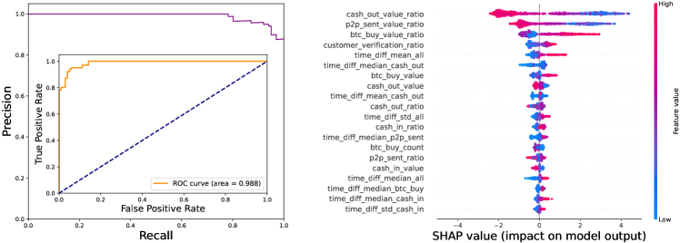
Figure 1: a) Precision-Recall and Receiver operating characteristic, ROC (inset) and b) SHAP (Lundberg and Lee 2017) analysis for our simple example binary classifier model. Model training and validation data were generated using the fintech-kMC tool. The full list of features used to train the model is listed in the online Supplementary Information.

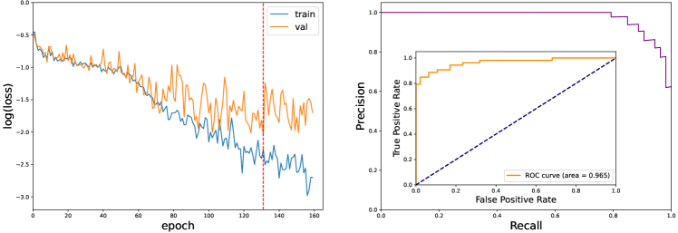
Figure 2: a) LSTM loss curves for train and validation sets b) Precision-Recall and ROC (inset) for the model (evaluated at epoch denoted by vertical red line). Hyperparameters are listed in the online Supplementary Information.

To demonstrate the utility of fintech-kMC with ML tools, here we show results from a toy experiment to detect and classify bad actors from regular customers. For this particular simulation, bad actors were configured to have a lower rate of ID verification success (50% compared to 75% for regular customers) and slightly different peer-to-peer money transfer behaviours (an average transfer amount of $5\pm$3 vs $8\pm$3 and a willingness to do such transfers only when their balance was above $15\pm$3 vs $30\pm$3). Here $\pm$ denotes the standard deviation of the normal distributions from which we sample to determine the specific transfer amounts. We created a population of 1000 agents where 50% were bad actors and the remaining were regular, healthy customers. Our simulation covered a time period of $\approx 8$ days, which, given the various rate constants we used, represents approximately 100 actions for each agent. We use the convention that a positive label is deleterious (e.g. a scam, an account take-over, or some other activity we wish to identify and prevent). To train a model, we constructed a series of features listed in the online Supplementary Information. We used a train-validation-test split of 80%-10%-10% and trained an XGBoost binary classifier (Chen and Guestrin 2016), Fig. 1, as well as an LSTM (Hochreiter and Schmidhuber 1997), Fig. 2, on the data (full model training hyperparameters are provided in the online Supplementary Information).

Limitations of the method

• Introducing new types of actions requires more software implementation. We cannot learn directly from data streams from our real-world system.

• Rate constant probability distributions in the control file are set manually by the user. To match them to a particular dataset, they must be optimized in a separate loop. Conceivably this could be achieved by automatic differentiation, but such capability is not currently included.

• Large scale network effects are currently not well described due to the small number of agents we typically simulate using the tool (e.g. 1k). In principle, agent-based kMC can be used to simulate larger “worlds” (e.g. 1-10M) but for simplicity we have not implemented the typical optimization or parallelization techniques needed to achieve such performance here.

• The current implementation is written in python. This is convenient for prototyping and adding new features, but results in a tool which is not as performant as it could be.

• In the current implementation, actions can occur at any time during the simulated day, whereas in real-world data customers tend to exhibit daily trends. This is not, however, a fundamental limitation of the methodology.

• Our positive labels are currently assigned at the customer level, rather than the individual transaction level. We are currently working to remove this restriction.

• Data produced by the model should not be seen as a source of data for production models.

Conclusions

fintech-kMC is an agent-based model which can simulate the behaviour of customers of online digital financial platforms. The tool implements many actions typical of such platforms, such as peer-to-peer money movements, ID verification, and crypto purchases. By using kinetic Monte Carlo, events occur at realistic timescales and can have meaningful sequential dependencies. Data produced by the tool can be used to test and validate machine learning workflows in a controllable and repeatable way.

Supplementary Information

Architexture details of our LSTM and XGBoost models are presented in Table S1 and Table S2. We also provide a list of the hand-designed features we used to train our feature-based ML models (Table S3).

base_score	0.5
booster	gbtree
colsample_bylevel	1
colsample_bynode	1
colsample_bytree	1
gamma	0
learning_rate	0.1
max_delta_step	0
max_depth	3
min_child_weight	1
missing	None
n_estimators	100
nthread	1
objective	binary$\colon$logistic
reg_alpha	0
reg_lambda	1
scale_pos_weight	1
seed	0
subsample	1
verbosity	1
tree_method	hist

Table 1: Parameters used to train our XGBoost (Chen and Guestrin 2016) model

Layer	Type	Output units	Dropout rate	Return sequence
0	Bidirectional LSTM	64	0.2	True
1	Bidirectional LSTM	64	0.2	True
2	Bidirectional LSTM	64	0.2	False
3	Dense	1

Table 2: Architexture (layer definitions) of our LSTM (Hochreiter and Schmidhuber 1997) neural network model

total_events

cash_in_count

customer_verification_count

cash_out_count

p2p_sent_count

btc_buy_count

cash_in_ratio

customer_verification_ratio

cash_out_ratio

p2p_sent_ratio

btc_buy_ratio

cash_in_value

customer_verification_value

cash_out_value

p2p_sent_value

btc_buy_value

cash_in_value_ratio

customer_verification_value_ratio

cash_out_value_ratio

p2p_sent_value_ratio

btc_buy_value_ratio

time_diff_mean_all

time_diff_median_all

time_diff_std_all

time_diff_mean_cash_in

time_diff_median_cash_in

time_diff_std_cash_in

time_diff_mean_customer_verification

time_diff_median_customer_verification

time_diff_std_customer_verification

time_diff_mean_cash_out

time_diff_median_cash_out

time_diff_std_cash_out

time_diff_mean_p2p_sent

time_diff_median_p2p_sent

time_diff_std_p2p_sent

time_diff_mean_btc_buy

time_diff_median_btc_buy

time_diff_std_btc_buy

Table 3: Hand-designed features we created and used as input to our XGBoost model

References

- Albergo, Kanwar, and Shanahan (2019) Albergo, M. S.; Kanwar, G.; and Shanahan, P. E. 2019. Flow-based generative models for Markov chain Monte Carlo in lattice field theory. Phys. Rev. D, 100: 034515.
- Chen and Guestrin (2016) Chen, T.; and Guestrin, C. 2016. XGBoost: A Scalable Tree Boosting System. In Proceedings of the 22nd ACM SIGKDD International Conference on Knowledge Discovery and Data Mining, KDD ’16, 785–794. New York, NY, USA: Association for Computing Machinery. ISBN 9781450342322.
- Ghosh et al. (2021) Ghosh, P.; Gupta, N.; Dhankhar, M.; and Ranganathan, M. 2021. Kinetic Monte Carlo simulations of self-organization of Ge islands on Si(001). Phys. Chem. Chem. Phys., 23: 19022–19031.
- Goodfellow et al. (2014) Goodfellow, I. J.; Pouget-Abadie, J.; Mirza, M.; Xu, B.; Warde-Farley, D.; Ozair, S.; Courville, A.; and Bengio, Y. 2014. Generative Adversarial Networks. .
- Hochreiter and Schmidhuber (1997) Hochreiter, S.; and Schmidhuber, J. 1997. Long Short-Term Memory. Neural Computation, 9(8): 1735–1780.
- Höfer et al. (2020) Höfer, S.; Bekris, K.; Handa, A.; Gamboa, J. C.; Golemo, F.; Mozifian, M.; Atkeson, C.; Fox, D.; Goldberg, K.; Leonard, J.; Liu, C. K.; Peters, J.; Song, S.; Welinder, P.; and White, M. 2020. Perspectives on Sim2Real Transfer for Robotics: A Summary of the R:SS 2020 Workshop. .
- Lundberg and Lee (2017) Lundberg, S.; and Lee, S.-I. 2017. A Unified Approach to Interpreting Model Predictions. .
- Papageorgiou and Paskov (1999) Papageorgiou, A.; and Paskov, S. H. 1999. Deterministic Simulation for Risk Management. The Journal of Portfolio Management, 25(5): 122–127.
- Ryczko et al. (2017) Ryczko, K.; Domurad, A.; Buhagiar, N.; and Tamblyn, I. 2017. Hashkat: large-scale simulations of online social networks. Social Network Analysis and Mining, 7(1): 4.
- Stamatakis and Vlachos (2012) Stamatakis, M.; and Vlachos, D. G. 2012. Unraveling the Complexity of Catalytic Reactions via Kinetic Monte Carlo Simulation: Current Status and Frontiers. ACS Catalysis, 2(12): 2648–2663.
- Voter (2007) Voter, A. F. 2007. Introduction to the kinetic Monte Carlo method. In Sickafus, K. E.; Kotomin, E. A.; and Uberuaga, B. P., eds., Radiation Effects in Solids, 1–23. Dordrecht: Springer Netherlands. ISBN 978-1-4020-5295-8.
- Wang (2012) Wang, H. 2012. Monte Carlo simulation with applications to finance. CRC Press.