Recursive classification of satellite imaging time-series:
An application to land cover mapping

Abstract

A wide variety of applications of fundamental importance for security, environmental protection and urban development need access to accurate land cover monitoring and water mapping, for which the analysis of optical remote sensing imagery is key. Classification of time-series images, particularly with recursive methods, is of increasing interest in the current literature. Nevertheless, existing recursive approaches typically require large amounts of training data. This paper introduces a recursive classification framework that improves the decision-making process in multitemporal and multispectral land cover classification algorithms while requiring low computational cost and minimal supervision. The proposed approach allows the conversion of an instantaneous classifier into a recursive Bayesian classifier by using a probabilistic framework that is robust to non-informative image variations. Three two-class experiments are conducted using Sentinel-2 data. The first one consists in the water mapping of an embankment dam in Oroville, California, USA; the second one is a water mapping experiment of the Charles river basin area in Boston, Massachusetts, USA; and the last experiment addresses deforestation detection in the Amazon rainforest. The spectral index classifier (SIC) is introduced as a method to convert broadband spectral indices such as the Normalized Difference Water Index (NDWI) and the Modified NDWI (MNDWI) into probabilistic classification results. A classifier based on the Gaussian mixture model (GMM), a logistic regression (LR) classifier, and the SIC are compared to their recursive counterparts. Results show that the use of Bayesian recursion significantly increases the robustness of existing instantaneous classifiers in multitemporal settings, including two state-of-the-art deep learning-based models, without the need for additional training data. Furthermore, the proposed framework scales well for an increasing number of classes.

[inst1]organization=Northeastern University,city=Boston, postcode=02215, state=MA, country=USA

[inst2]organization=CRAN, University of Lorraine, CNRS,city=Vandoeuvre-les-Nancy, postcode=F-54000, country=France

1 Introduction

For the purpose of allaying increasing concerns on global environmental changes and sustainability, and thanks to the vast amount of high resolution remotely sensed data available today, there exists a considerable body of work focused on remote sensing applications involving land cover mapping and change detection (Anderson, 1976; Srivastava et al., 2012; Rwanga et al., 2017; Karan and Samadder, 2018). Some application examples are studies on land conservation, sustainable development, landscape planning and management of resources such as, e.g., water. Changes in water dynamics can be studied by surface water mapping, with the aim of monitoring floods (Proud et al., 2011; Koukoula et al., 2020; Farhadi et al., 2022), describing water quality (Jiang et al., 2020; Son and Wang, 2020; Tong et al., 2010), or for coastline extraction and change assessment (Ekercin, 2007; Pardo-Pascual et al., 2012; Hannv et al., 2013; Zhang et al., 2013). Land cover mapping is of fundamental importance when identifying the distribution of different types of crops (Griffiths et al., 2019; Tewabe and Fentahun, 2020) or the dynamical evolution of land use in urban environments (Gadrani et al., 2018; Liu et al., 2018). Another interesting case of study, which we focus on for the analysis of the proposed algorithm, is the detection of deforestation in areas such as the Amazon rainforest, where the greatest share of deforestation in the world is alarmingly taking place. This region is recognized as the largest tropical rainforest globally and is known for its unparalleled biodiversity and crucial role in global climate regulation. Numerous works in the literature have been addressing the environmental impact and contribution to climate change of deforestation in the Amazon for several decades (Lean and Warrilow, 1989; Shukla et al., 1990). Human activities such as agricultural expansion, mining, and land clearing have led to widespread habitat loss, fragmentation, and alterations in the ecosystem, impacting numerous plant and animal species (Mulatu et al., 2017). Satellite remote sensing is a fundamental tool to monitor these phenomena, especially in areas of that are difficult to access (Cha et al., 2023).

Several sources of remotely sensed data are currently available, presenting different characteristics when it comes to spatial, spectral, radiometric and temporal resolution (Satir and Berberoglu, 2012; Zhu et al., 2022). Spatial resolution typically varies from centimeters, in the case of very high resolution sensors, such as the ones in the GeoEye and QuickBird-2 satellites, to a few meters, in the case of sensors used by the Landsat 9 and Sentinel-2 A/B satellites. Such satellites can acquire images of the same scene with a weekly temporal resolution. On the other hand, satellites equipped with the moderate resolution imaging spectroradiometer (MODIS) and the visible infrared imaging radiometer suite (VIIRS) sensors achieve a higher temporal resolution, with daily image acquisitions. However, their spatial resolution is significantly lower, being in the order of hundreds of meters. There are modern commercial satellite systems designed for a range of very high resolution remote sensing applications that push the boundaries of Earth observation. An example is the Pléiades Neo by Airbus, with a twice-daily revisit capacity and up to 30 cm of ground sampling distance (Chouteau et al., 2022). It is relevant to point out the availability of hundreds of CubeSats with subweekly or even daily temporal resolution and medium to high spatial resolution (Zhu et al., 2022), such as the ones providing Planetscope data (Huang and Roy, 2021). Also, very high resolution optical imagery is available with the constellations of SkySat, BlackSky and Nu-Sat micro-satellites, which are based on the CubeSat concept. The SkySat satellites can provide ground sampling distances of up to 50 cm, a sub-daily revisit time (6-7 times per day) when considering the whole constellation, and a 4-5 revisit time when considering individual satellites  (Jacobsen, 2022). In order to combine images with different spatial and temporal resolutions, multimodal image fusion techniques have been developed to generate high spatio-temporal image sequences, contributing to generating a wealth of remotely sensed data (Zhu et al., 2010, 2018; Li et al., 2022).

Spectral indices are one of the main land cover mapping tools given their simplicity and required low computational cost. They compute scalar-valued features as a function of specific spectral bands, whose value can be used to distinguish between different land cover classes contained in a pixel. Although they show a limited performance when compared to other techniques such as deep learning methods, they are widely used in remote sensing applications given their unsupervised nature (Khalid et al., 2021). They can be considered to be unsupervised because their output depends on the ratio between a combination of spectral bands, which does not require any training. The decision threshold, however, must be selected and this can be challenging when no reference data is available. Another advantage of these methods is that spectral index values can be easily interpreted or explained, as they minimize the effect of illumination in satellite imagery while enhancing different spectral features present in the scene under study. For instance, the Normalized Difference Vegetation Index (NDVI) enhances the presence of trees, bushes, and others. This is due to the reflectance given by the spectral response of vegetation decreasing in the red and increasing in the infrared wavelengths. On the other hand, water indices are used for water extraction at pixel level, given the difference in spectral reflectance of land and water in the near and middle infrared wavelengths (Xie et al., 2016). The most widely used water indices are the Normalized Difference Water Index (NDWI), the Modified NDWI (MNDWI) and the Automated Water Extraction Index (AWEI) (Acharya et al., 2018). It has been shown that challenging weather conditions may disrupt the extraction of water bodies with these indices. This can be solved by using modified methods like the one proposed by Gao et al. (2016), which effectively mitigates mountain shadows and allows the extraction of particularly challenging small water bodies. Khalid et al. (2021) also suggest that the Land surface temperature Based Water Extraction Index (LBWEI) provides high accuracy under a wide variety of weather conditions. Results in (Zhang et al., 2019) show that overall classification accuracy can be improved by processing all the available Sentinel-2A spectral bands instead of a subset of them.

Aside from spectral index methods, there is a wide choice of land cover classification approaches based on machine learning available in the literature, whose main advantage is an increased flexibility. The taxonomy of image classification techniques in remote sensing proposed by Satir and Berberoglu (2012) groups them into supervised/unsupervised, parametric/non-parametric and hard/soft classifiers, among others. Some of the explored machine learning methods used in remote sensing applications include maximum likelihood classifiers (Frazier and Page, 2000), support vector machines (Hannv et al., 2013), logistic regression (LR) (Mueller et al., 2015), random forests (Pelletier et al., 2016, 2017), naive Bayes and clustering methods like the widely used K-means algorithm. Manandhar et al. (2009) show that results obtained with the maximum likelihood classification of Landsat images can be improved by applying a post-classification correction using a hypothesis testing framework of knowledge engineer, where artificial intelligence comes into play. More recent works assess the need for an actual comparison between widely used machine learning algorithms when investigating land cover classification, proposing random forest as the best classification model in the mining district when compared to maximum likelihood, support vector machines, and classification and regression trees (Ko Oo et al., 2022). Furthermore, Skakun (2010) and Qiu et al. (2019) suggest that deep learning methods like artificial neural networks provide high accuracy results in land cover classification, even when compared to other machine learning classifiers such as support vector machines.

Despite their widespread use in land cover mapping, the previously mentioned techniques suffer from several limitations. First, they are highly sensitive to illumination and atmospheric interferences (e.g., different aerosol concentrations or viewing angles), which can significantly impact the spectra of pixels from a given material class (Theiler et al., 2019; Borsoi et al., 2021b). The lack of robustness to such non-informative spectral variations is a significant limitation of, for instance, spectral indices such as the MNDWI (Yang et al., 2018). Moreover, due to the high sensor-to-target distances involved in remote sensing applications, many image pixels do not belong to a single class, but are instead composed of a mixture of different material classes (Quintano et al., 2012). Although this can be addressed by spectral mixture analysis techniques (Keshava and Mustard, 2002) or by assigning a pixel to more than one class (Mertens et al., 2006), it poses a significant challenge to traditional classification algorithms. As a consequence, an apparent need for robustness to outliers and spurious artifacts in remotely sensed data arises.

The analysis of multitemporal or time-series data is of increasing interest for remote sensing applications (Kuenzer et al., 2015; Johnson and Iizuka, 2016). Exploiting multitemporal data makes it possible to improve the performance of tasks such as classification (Gómez et al., 2016; Deng et al., 2019) or spectral mixture analysis (Halabisky et al., 2016; Borsoi et al., 2021a) due to its temporal correlation, while at the same time supplying the end-user with a more complete product that shows the spatial as well as the temporal distribution of land classes or their proportions. The simplest approach to perform multitemporal land cover mapping is to apply an instantaneous classifier to each image in the sequence, being spectral indices such as the NDVI a popular choice (Jeevalakshmi et al., 2016; Sun et al., 2018). However, this does not exploit the temporal information available in the data. Significant effort has been dedicated to developing techniques specifically suited to process multitemporal image sequences. For instance, Hoberg et al. (2015) and Kenduiywo et al. (2017) proposed classification methods based on conditional random field models, which represent the interactions between class labels in both time and space. Transfer and active learning were combined by Demir et al. (2013) to adapt a pre-trained classifier to new images acquired at other time instants. Time-series classification accounting for missing pixels using Gaussian process regression was proposed by Constantin et al. (2022), while other works considered 1D temporal covolutional neural networks (CNNs) (Pelletier et al., 2019), and 3D spatio-temporal CNNs (Ji et al., 2018).

The aforementioned techniques require a full image time-series as input in order to produce classification maps, and are thus often referred to as batch or offline time-series classification methods. However, in practice, instruments such as Sentinel-2 or Landsat 9 are continuously acquiring images. Generating classification maps online using batch algorithms require re-processing the whole image time-series every time a new image is acquired, which can be computationally expensive. On the other hand, recursive methods, which may also be referred to as online methods, allow to iteratively update multitemporal classification maps as new images are acquired by leveraging previously computed results. Consequently, these methods have a natural appeal in studies where data collection is performed over time. For instance, Bayesian recursion is widely used in target tracking applications, where an efficient filter (Imbiriba and Closas, 2020) must be designed to recursively obtain target state estimates from a state-space model (Ji et al., 2022). Filtering methods can also be used to develop online parameter learning (Wu et al., 2019; Borsoi et al., 2020; Demirkaya et al., 2021; Imbiriba et al., 2022), which is of special interest in machine learning tasks involving the processing of time-series data (Campbell et al., 2021), such as video prediction (Schneider and Gavrila, 2013; Gujjar and Vaughan, 2019) and speech enhancement (Cohen and Berdugo, 2002; Martín-Doñas et al., 2020). Interestingly, Bayesian recursion has been applied to pattern recognition for bioengineering applications, such as in Uslu and Bharath (2019), where they track retinal vasculature by estimating vessel geometry parameters. It is worth mentioning other works from the fields of precise navigation, such as (Closas et al., 2009), where multipath in GNSS receivers is mitigated with a Bayesian recursive approach, or the recent (Medina et al., 2020), where the joint estimation of position and attitude in a GNSS multi-antenna system is enhanced.

The earliest recursive remote sensing classification techniques were based on Bayesian filtering ideas, by recursively updating the probabilities of each class given the measurements after each datum is acquired (Swain, 1978; Strahler, 1980). These techniques are based on a statistical model that represents the pixel spectra given its class, called a generative model, which is non-trivial to obtain. More recent Bayesian approaches have proposed classification strategies that are recursive both in time, and across multiple spatial scales (multiresolution) (Hedhli et al., 2016), using computationally expensive algorithms such as the expectation maximization method to learn parameters and a generative model for the pixels. Other recent works have leveraged deep learning strategies, in particular different instantiations of recurrent neural networks, such as long short-term memory (LSTM) networks. These have been applied to predict flood susceptibility and for crop identification, among others (Rußwurm and Korner, 2017; Fang et al., 2021). The methods proposed in these works allow the learning of intrinsic spatial and temporal dependencies of remotely sensed data, together with spectral patterns in specific classes over different time instants. They achieve this with minimal supervision, providing significant improvements in classification accuracy. In the context of land cover classification, the main disadvantage of other recursive algorithms, such as the one in (Sharma et al., 2018) using patch-based recurrent neural networks, is that they need large amounts of training data and long training times when compared to the proposed RBC framework. Mountrakis and Heydari (2023) show that deep learning methods provide substantial classification improvements over the commonly implemented random forest. Nevertheless, demonstrative numbers on simulation times suggest that these methods require up to four times larger running times. With the framework proposed in this paper, we aim to provide an improvement in classification tasks while assessing data patterns over time, and without the computational load of a deep learning algorithm.

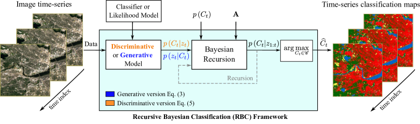
Figure 1: Overview of the proposed recursive Bayesian classifier. This method is able to convert an instantaneous generative model (i.e., which models the observation of a pixel given its class label with the likelihood function $p\left(\boldsymbol{z}_{t}|C_{t}\right)$) or a discriminative model (i.e., which models the observation of a class label given a corresponding pixel with $p\left(C_{t}|\boldsymbol{z}_{t}\right)$) into a recursive Bayesian classifier that exploits the temporal relationship of time-series data. Knowledge about the state transition matrix $\mathbf{A}$ and the class prior probabilities $p\left(C_{t}\right)$ is assumed. The hat operator in $\widehat{C}_{t}$ denotes the decision from the classifier. Finally, $\mathscr{C}$ is an experiment-dependent set containing $K$ different labels.

The aim of this paper is to develop a recursive classification framework that improves the decision-making process in multitemporal and multispectral land cover classification algorithms by leveraging previous classification results. With the proposed approach, termed recursive Bayesian classification (RBC), we aim to address the trade-off between adaptability to natural changes in the scene and robustness to outliers caused by illumination variations and spurious artifacts in remotely sensed data. This is performed without the need for large amounts of training data, as opposed to deep learning models, which need huge training datasets. The RBC framework converts an instantaneous generative model (i.e., which models the observation of a pixel given its class label) or discriminative classifier (i.e., which models the observation of a class label given a corresponding pixel) into a recursive classifier using a probabilistic framework. This integration of existing state-of-the-art instantaneous classification algorithms differs from previous approaches based on generative models (Swain, 1978; Strahler, 1980; Hedhli et al., 2016). An overview of the method introduced in this paper can be found in Fig. 1. The underlying likelihood or class posterior models to which the RBC framework is applied may be either semi-supervised, supervised or unsupervised. Consequently, when we discuss the training stage methodology in Section 3.3.2, we are specifically referring to the training of the selected instantaneous algorithms that require supervision, not to the RBC framework itself. The proposed method is based on a Markov assumption on the transition of the class labels, which states that the probabilities of a change in a class label can be determined based only on the information of labels at the most recent time instants. This simplifies the model and allows to capture the dynamical aspect of the classifier with the hyperparameter that defines the class transition probabilities. This hyperparameter can be tweaked to balance the capability of the classifier to adapt to class changes with the increase of its robustness to non-informative spectral variations originating from, e.g., atmospheric and illumination variations.

An implicit regularization of the instantaneous classifiers class probabilities is proposed in Section 3.1.4 to address overconfident classification results which are common in models such as, e.g., deep neural networks. When the instantaneous classifiers are overconfident, the influence of the prior information from past time instants is greatly reduced, thus overturning the recursive nature of the framework. This makes implicit regularization an important element of RBC in order to preserve both the adaptability and robustness of the algorithms. Furthermore, we introduce the spectral index classifier (SIC) in Section 3.2, where standard broadband indices are converted into predictive probabilities to calculate the probability mass function (PMF), which gives information about the class prediction uncertainty and can therefore be integrated into the RBC framework.

The performance of the proposed approach is demonstrated using Sentinel-2 images. The first experiment consists in the water mapping of a reservoir and its downstream river, in Oroville, California, USA. The two regions selected for evaluation pose several challenges to water mapping algorithms, such as ripples caused by changes in the water flow, variations in illumination, and abrupt changes in the water level of the reservoir. The second experiment focuses on the water mapping of the Charles river basin, in Boston, Massachusetts, USA. This region is also challenging given the appearance of algal blooms in the summer, variations in illumination and in atmospheric conditions, and the presence of highly reflective surfaces. The last experiment aims to detect deforestation in the Amazon rainforest. Three instantaneous classifiers are compared to their recursive counterparts, including a classifier based on the Gaussian mixture model (GMM), an LR classifier, and the SIC algorithm. For the water mapping experiments, we also included as benchmark models two pre-trained state-of-the-art deep learning classifiers. These are the DeepWaterMap (Isikdogan et al., 2017) and WatNet (Luo et al., 2021) algorithms. When the RBC framework is applied atop a generative model like GMM, the method is denoted as Recursive Bayesian Classification based on a Generative Model (RBGM), discussed in Section 3.1.1. Conversely, when applied atop discriminative models like LR or SIC classifiers, it is termed Recursive Bayesian Classification based on a Discriminative Model (RBCD), discussed in Section 3.1.2.

The lack of open-source labeled Sentinel-2 data for time-series analysis (i.e., containing the dynamical evolution of the true class labels) poses an important challenge to the evaluation of the methods. Although there are available multitemporal satellite imagery datasets, most of them contain pixel-wise annotations that are unique for the whole time-series. That is, no changes over time exist or are properly mapped to labels, and therefore, it is not possible to evaluate the algorithm at different time instants. One example of this is the benchmark dataset for multi-temporal and multi-modal land use land cover mapping MultiSenGE (Wenger et al., 2022). To address this issue, we manually generated water labels of the two areas under study in the Oroville Dam region and the Charles river basin for the two water mapping experiments. For the Amazon deforestation experiment, ground truth labels were obtained from the MultiEarth challenge dataset (Cha et al., 2023).

The remainder of this paper is structured as follows. Section 2 describes the satellite data and the study area. Section 3 introduces the proposed RBC framework and the SIC algorithm, followed by details on the experimental setup. Section 4 presents the results, while the implications and impact are discussed in Section 5. Finally, Section 6 provides the concluding remarks. The successful extension of the RBC framework to a three-class classification task for the Charles River area is detailed in Appendix A.

2 Area of study and satellite data

Our research focuses on two areas of study located in the US and one area located in the Amazon rainforest, as we believe it is essential to test our methodology across varied geographical locations to achieve a more comprehensive performance assessment. In this section, we describe the three selected areas of study and the challenges they pose to land cover mapping algorithms. We consider images at the blue, green, red, near-infrared (NIR), narrow NIR and shortwave infrared (SWIR) bands, with resolution and central wavelength listed in Table 1. Band 4 (red) is useful for identifying soil, water and many urban features, band 3 (green) gives excellent contrast between clear and turbid waters, and band 2 (blue) is useful for identifying vegetation and also human-made features (Maciej Huk, 2020). The SWIR bands are useful for measuring vegetation, water and soil moisture.

Table 1: Resolution and central wavelength of the processed Sentinel-2 spectral bands.

Band	Description	Resolution (m)	Central wavelength (nm)
2	Blue	10	490
3	Green	10	560
4	Red	10	665
8	NIR	10	842
8A	Narrow NIR Edge	20	865
11	SWIR 1	20	1610

2.1 Test site 1: Oroville Dam

The first test site is located in Oroville Dam, an embankment dam on the east side of the city of Oroville, in the state of California (see Fig. 2). Being 235 meters high, it is the tallest dam in the US. The area of study has geographic center coordinates of LAT/LON: 39.61, -121.43. Test sites 1a and 1b belong to the dam downstream and upstream, respectively. Water mapping of areas with geographic features like this reservoir is imperative to study, as they are used for flood control, management and sustainability of water resources.

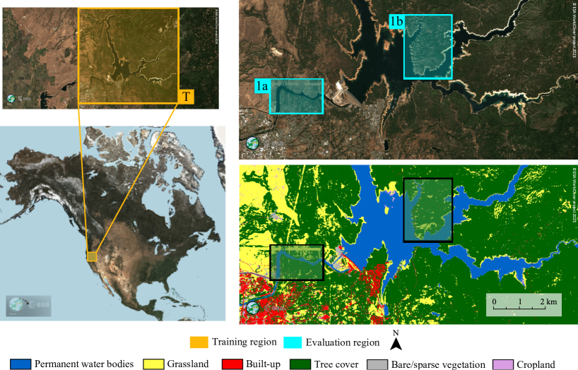
Figure 2: Sentinel-2 RGB composite images and classification map from the ESA WorldCover Map tool (Zanaga et al., 2021) of test sites 1a and 1b (Oroville Dam, California, USA).

Illumination variations in images from test site 1a can be observed in Fig. 4. These may be caused by fluctuations in the solar incidence angle and also by differences in image acquisition times. Ripples and other artifacts in test site 1a are caused by the high flows in the river stream, making the classification of water pixels challenging and increasing the probability of false negatives. As illustrated in Fig. 4 for test site 1b, and based on reservoir storage data obtained from the NWIS USGS website , the water level in the reservoir changes abruptly with the season. In October 2020, the recorded water storage was of 200,485.8 hc-m, decreasing to 160,783.2 hc-m in December 2020. Subsequent changes resulted in a recorded water storage of 183,223.8 and 97,542.6 hc-m in May and September of 2021, respectively. These phenomena demand the flexibility of the proposed recursive classification framework, which ensures its ability to adapt to changes in the scene. However, the very high flexibility of the method can put its robustness at risk.

Sentinel-2 Level-2A images are downloaded using the Google Earth Engine platform from the COPERNICUS/S2_SR collection, with dates between 2020-09-01 and 2021-09-26. This platform atmospherically corrects the images using the standard SEN2COR software package and indicates a cloud cover percentage. Only images with at most 10% cloud cover are downloaded. The downloaded images have dimensions of $2229\times 3341$ pixels. For evaluation purposes, images were cropped to sizes of $200\times 500$ pixels for test site 1a and $150\times 110$ pixels for test site 1b. To ensure consistency, images from bands 8A and 11, initially at a resolution of 20 meters, were resampled to 10 meters using nearest-neighbor interpolation. A total of 45 images remained available for further processing.

2.2 Test site 2: Charles river basin

The area of study for this experiment covers the Charles river, the Mystic river and the Boston harbor in Massachusetts, with geographic center coordinates of LAT/LON: 42.36, -71.12 (see Fig. 3). This location includes a big permanent water body, urban vegetation, and a built-up area, which makes it a site of interest for land cover classification. Tracking land cover changes in urban environments is of great help for urban and agriculture planning, and also when trying to identify correlations between social activities and land changes. Challenges in test site 2 include illumination variations (see Fig. 4) and the presence of reflective surfaces from buildings and seasonal cyanobacterial blooms in the Charles river and in the Boston harbor waters. Algal blooms mostly occur during summer (Rome et al., 2021), as in the image captured on 2021-07-31 shown in Fig. 4.

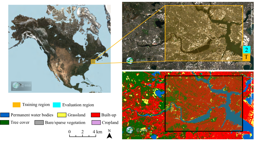
Figure 3: Sentinel-2 RGB composite images and classification map from the ESA WorldCover Map tool (Zanaga et al., 2021) of test site 2 (Charles river, Boston, USA).

Sentinel-2 Level-2A images are downloaded using the Google Earth Engine platform from the COPERNICUS/S2_SR collection, with dates between 2020-09-04 and 2021-09-29. Only images with at most 10% cloud cover are downloaded. The downloaded images have dimensions of $927\times 2041$ pixels. For evaluation purposes, images were cropped to sizes of $700\times 1241$ pixels. Images from bands 8A and 11 are resampled to 10 meters by nearest-neighbor interpolation. After visual inspection, 15 images depicting snow-covered land or exhibiting significant disparities are excluded from the dataset, resulting in a total of 28 images for further processing.

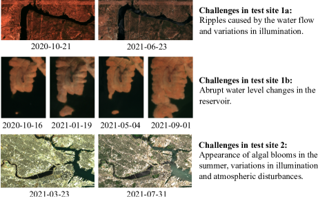
Figure 4: Sentinel-2 RGB composite images showing the challenges posed by test sites 1a, 1b, and 2, within the context of water mapping and land cover classification.

2.3 Test site 3: Amazon rainforest

The third experiment focuses on the geographic area of the Amazon rainforest in Brazil, at the geographic center coordinates LAT/LON: -4.05, -54.6 (see Fig. 5). Sentinel-2 images of the Amazon rainforest downloaded using the Google Earth Engine platform are obtained from the MultiEarth challenge dataset (Cha et al., 2023). For some dates, this dataset includes manually generated deforestation labels using mosaic satellite images from the Planet APIs. We initially consider a total of 225 images with dates between 2018-12-03 and 2021-12-27. These have the same dimensions as the MultiEarth dataset images after being tiled and segmented, i.e., $256\times 256$ pixels. The study area is selected to be relatively small in order to ease the analysis of results since the evolution in time of output classification maps can be more easily interpreted for smaller regions. Also, the overall computational cost decreases when lowering the number of pixels to be evaluated.

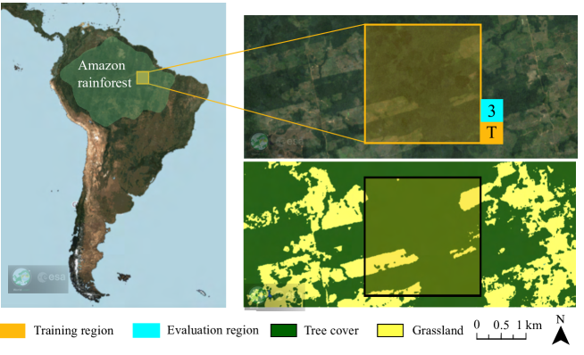
Figure 5: Sentinel-2 RGB composite images and classification maps from the ESA WorldCover Map tool (Zanaga et al., 2021) of test site 3, located in the endangered Amazon rainforest.

The percentages of cloud and cloud shadow are calculated with the CI₂ and CSI indices proposed by Zhai et al. (2018). From the initially 225 selected images, the ones with a cloud/shadow cover above 20% are filtered out. We also discard 12 images by visual inspection. This results in a total of 31 images for further processing. Pixel values are scaled accordingly such that surface reflectance values are between 0 and 1. Also, these are shifted under the presence of clouds or illumination factors. To solve this, a time-varying bias is fitted to each image, for which an area where the statistics are expected to be time-invariant (i.e., no clouds or disturbances are observed inside that area for all evaluation dates) is selected. Taking the first evaluation image as a reference, the mean $\bar{x}_{\text{ref}}$ of pixel values inside that area is calculated. For each subsequent image, a bias is computed as $b(t)=\bar{x}_{\text{ref}}-\bar{x}_{\text{test}}(t)$ and applied in the pre-processing stage so that the pixel mean in the selected region is the same for all time instants. With this procedure, pixel values corresponding to the surface reflectance are not altered by the presence of clouds or other atmospheric effects.

Even after the detection and filtering of images with a relatively high cloud percentage, scenes in the Amazon rainforest often show a large number of small clouds, which may disrupt instantaneous classification. On the one hand, this demands the robustness of the proposed RBC framework. On the other hand, the temporal variability of the spectra of both vegetated and, especially, deforested areas, requires flexibility in the algorithm. This variability can be observed in the Sentinel-2 RGB composite images from dates 2019-08-10 and 2020-06-10 in Fig. 13. Overall, the proposed framework must address a trade-off between adaptability and robustness to surpass these challenges.

3 Methodology

The main contribution of this manuscript is the framework for recursive Bayesian classification using multispectral and multitemporal data, which is introduced in Section 3.1. We also propose, in Section 3.2, a classifier that uses spectral indices to generate predictive class probabilities. The experimental setup is described in Section 3.3.

3.1 Algorithm: recursive Bayesian classification (RBC)

Let us denote by $\boldsymbol{Z}_{t}\in\amsmathbb{R}^{B\times N}$ an image with $B$ bands and $N$ pixels observed at time instant $t=\{1,\ldots,T\}$. The images at the different time instants are supposed to be coregistered, that is, they constitute observations of the same geographic scene. For each pixel $\boldsymbol{z}_{t,n}\in\amsmathbb{R}^{B}$, being $n=\{1,\ldots,N\}$, we associate a label $C_{t,n}\in\mathscr{C}$, where $\mathscr{C}$ is an experiment-dependent set containg the possible $K$ labels. For a set of images $\boldsymbol{Z}_{t}$ over time, the most likely label $C_{t,n}$ for each pixel $\boldsymbol{z}_{t,n}$ (i.e., the $n$-th column of $\boldsymbol{Z}_{t}$) can be estimated based on all the previously observed data $\{\boldsymbol{Z}_{t},\boldsymbol{Z}_{t-1},\ldots,\boldsymbol{Z}_{1}\}$ by maximizing the posterior probability $p(C_{t,n}|\boldsymbol{Z}_{t},\boldsymbol{Z}_{t-1},\ldots,\boldsymbol{Z}_{1})$ as

$$\widehat{C}_{t,n}=\arg\max_{C_{t,n}\in\mathscr{C}}\,\,p(C_{t,n}|\boldsymbol{Z}_{t},\boldsymbol{Z}_{t-1},\ldots,\boldsymbol{Z}_{1})\,,$$ (1)

where the hat operator denotes the decision from the classifier. This expression is powerful, as it considers both temporal and spatial information. However, learning the posterior PMF in Eq. (1) can be hard, especially with high dimensional images. A spatial independence assumption can be applied to reduce the computational cost when calculating the conditional PMF. We propose to treat the label of every pixel as independent of the data from other pixels, meaning that $C_{t,n}$ only depends on $\boldsymbol{z}_{t,n},\boldsymbol{z}_{t-1,n},\ldots,\boldsymbol{z}_{1,n}$, or, equivalently, on $\boldsymbol{z}_{1:t,n}\triangleq\{\boldsymbol{z}_{t,n},\boldsymbol{z}_{t-1,n},\ldots,\boldsymbol{z}_{1,n}\}$. This is without loss of generality, as the proposed approach can be directly extended to consider spatial information (i.e., from multiple pixels). Thus, the posterior in Eq. (1) becomes $p(C_{t,n}|\boldsymbol{z}_{1:t,n})$, disregarding spatial information, and leading to

$$\widehat{C}_{t}=\arg\max_{C_{t}\in\mathscr{C}}\,\,p(C_{t}|\boldsymbol{z}_{1:t}),$$ (2)

where the pixel index $n$ is omitted for simplicity. The classifier proposed in Eq. (2) still considers a temporal dependence on previous data, meaning that the labels and images at previous time instants influence the results of the current time $t$. With the framework we propose, recursion can be applied to generative models, as in Section 3.1.1, and to discriminative models, as in Section 3.1.2.

3.1.1 Classification based on a generative model (RBGM)

The posterior PMF in Eq. (2) can be computed recursively using Bayes theorem under conditional independence assumptions and assuming knowledge about the prior $p(C_{0})$, the sate transition $p(C_{t}|C_{t-1})$ and the likelihood distribution $p(\boldsymbol{z}_{t}|C_{t})$. Thus, the posterior PMF can be computed as

$$\begin{split}p(C_{t}|\boldsymbol{z}_{1:t})&=\sum_{C_{t-1}\in\mathscr{C}}p(C_{t},C_{t-1}|\boldsymbol{z}_{1:t})\\ &\mathop{=}^{(a)}\sum_{C_{t-1}\in\mathscr{C}}p(C_{t}|C_{t-1},\boldsymbol{z}_{t})p(C_{t-1}|\boldsymbol{z}_{1:t-1})\\ &\mathop{=}^{(b)}\sum_{C_{t-1}\in\mathscr{C}}\frac{p(\boldsymbol{z}_{t}|C_{t})p(C_{t}|C_{t-1})}{p(\boldsymbol{z}_{t}|C_{t-1})}p(C_{t-1}|\boldsymbol{z}_{1:t-1})\\ &=p(\boldsymbol{z}_{t}|C_{t})\sum_{C_{t-1}\in\mathscr{C}}\frac{p(C_{t}|C_{t-1})}{\sum_{C_{t}^{\prime}}p(\boldsymbol{z}_{t}|C_{t}^{\prime})p(C_{t}^{\prime}|C_{t-1})}p(C_{t-1}|\boldsymbol{z}_{1:t-1}).\end{split}$$ (3)

where in equality $(a)$ we assumed a first-order Markov model, that is, given $C_{t-1}$ and $\boldsymbol{z}_{t}$, the class labels $C_{t}$ are independent of $\boldsymbol{z}_{1:t-1}$; in equality $(b)$ we applied the Bayes theorem followed by the same conditional independence assumption. We refer to the method in Eq. (3) as recursive Bayesian classification based on a generative model (RBGM) due to its dependence on the likelihood function $p(\boldsymbol{z}_{t}|C_{t})$. The term $p(C_{t-1}|\boldsymbol{z}_{1:t-1})$ denotes the posterior PMF of the previous time step. This term shows in the equation because states are assumed to be independent of future measurements, meaning that $C_{t-1}$ depends on $\boldsymbol{z}_{1:t-1}$ but not on $\boldsymbol{z}_{t}$. When $t=1$, $p(C_{t-1}|\boldsymbol{z}_{1:t-1})$ becomes equivalent to the class prior probabilities since $p(C_{0}|\boldsymbol{z}_{0})=p(C_{0})$.

Eq. (3) uses the Bayes theorem, where the posterior probability is given by the product of the likelihood and the prior divided by the marginal probability. The denominator in this expression considers the probability of all the possible transitions that a pixel can go through. The transition PMF $p(C_{t}|C_{t-1})$ is described later in this section.

3.1.2 Classification based on a discriminative model (RBDM)

The posterior probability can also be computed as a function of the probability of the labels given the pixel values, which allows existing classification algorithms to be used in the RBC framework. In this case, the posterior probability is computed by following Eq. (5) and this is referred to as recursive Bayesian classification based on a discriminative model (RBDM). Applying the Bayes theorem to the likelihood $p(\boldsymbol{z}_{t}|C_{t})$ we obtain

$$p(\boldsymbol{z}_{t}|C_{t})=\frac{p(C_{t}|\boldsymbol{z}_{t})p(\boldsymbol{z}_{t})}{p(C_{t})},$$ (4)

where $p(C_{t}|\boldsymbol{z}_{t})$ is the prediction of the classifier to which the RBC framework is applied, which we refer to as a benchmark classifier. As the RBC framework is agnostic to the classifier that is used, the prediction can be the result of any type of classifier, including deep learning methods as well. The Bayes theorem can be used to extend RBGM to RBDM as

$$\begin{split}p(C_{t}|\boldsymbol{z}_{1:t})&=\frac{p(C_{t}|\boldsymbol{z}_{t})p(\boldsymbol{z}_{t})}{p(C_{t})}\sum_{C_{t-1}\in\mathscr{C}}\frac{p(C_{t}|C_{t-1})}{\sum_{C_{t}^{\prime}}p(\boldsymbol{z}_{t}|C_{t}^{\prime})p(C_{t}^{\prime}|C_{t-1})}p(C_{t-1}|\boldsymbol{z}_{1:t-1})\\ &=\frac{p(C_{t}|\boldsymbol{z}_{t})\cancel{p(\boldsymbol{z}_{t}})}{p(C_{t})}\sum_{C_{t-1}\in\mathscr{C}}\frac{p(C_{t}|C_{t-1})}{\sum_{C_{t}^{\prime}}\frac{p(C_{t}^{\prime}|\boldsymbol{z}_{t})\cancel{p(\boldsymbol{z}_{t})}}{p(C_{t}^{\prime})}p(C_{t}^{\prime}|C_{t-1})}p(C_{t-1}|\boldsymbol{z}_{1:t-1})\\ &=\frac{p(C_{t}|\boldsymbol{z}_{t})}{p(C_{t})}\sum_{C_{t-1}\in\mathscr{C}}\frac{p(C_{t}|C_{t-1})}{\sum_{C_{t}^{\prime}}\frac{p(C_{t}^{\prime}|\boldsymbol{z}_{t})}{p(C_{t}^{\prime})}p(C_{t}^{\prime}|C_{t-1})}p(C_{t-1}|\boldsymbol{z}_{1:t-1}),\end{split}$$ (5)

where $p(C_{t})$ denotes the marginal class probability. In the widely used naive Bayes classifier, the marginal class probabilities are also used (Barber, 2011). In the absence of labeled training data and prior information about the scene, we set their value as $p(C_{t})=\frac{1}{K}\;\forall~{}C_{t}$.

Note that the proposed recursive classification solution is in closed-form and consists of a summation of probability distributions over the different classes. Eqs. (3) and (5) are straightforward to compute given the likelihood of the pixels or their posterior probability, respectively, which correspond to the result of the instantaneous classifier. Considering this, it can be stated that recursion does not add a significant computational overhead to the classification problem.

3.1.3 Class transition probabilities

The term $p(C_{t}|C_{t-1})$ in Eqs. (3) and (5) corresponds to the state transition probability, which can be described using the so-called state transition probability matrix. For simplicity, in this work, we assume $p(C_{t}|C_{t-1})$ to be time invariant. Although strong, this assumption copes with the lack of knowledge we assume regarding the studied scene. We highlight, however, that this is so without loss of generality since prior knowledge about, e.g., seasonality, can be easily incorporated in a time-dependent transition PMF. Being $p_{ij}=p(C_{t}=j|C_{t-1}=i)$, this matrix can be expressed for $K$ classes as

$$\mathbf{A}=\begin{bmatrix}p_{11}&p_{12}&\ldots&p_{1K}\\ p_{21}&p_{22}&\ldots&p_{2K}\\ \vdots&\vdots&\ddots&\vdots\\ p_{K1}&p_{K2}&\ldots&p_{KK}\end{bmatrix}=\begin{bmatrix}1-(K-1)\epsilon&\epsilon&\ldots&\epsilon\\ \epsilon&1-(K-1)\epsilon&\ldots&\epsilon\\ \vdots&\vdots&\ddots&\vdots\\ \epsilon&\epsilon&\ldots&1-(K-1)\epsilon\end{bmatrix},$$ (6)

where it has been assumed that $p_{ij}=\epsilon$ for all $i\neq j$. The particular case of $K=2$ for the conducted experiments is shown in Eq. (7). This matrix is site-dependent and may be filled by expert judgment by selecting the proper value of $\epsilon$, which corresponds to the probability of a pixel transitioning from one label to another. A study on the model sensitivity to this hyperparameter is presented in Section 4.3.

$$\mathbf{A}|_{K=2}=\begin{bmatrix}1-\epsilon&\epsilon\\ \epsilon&1-\epsilon\end{bmatrix}\,.$$ (7)

3.1.4 Implicit regularization of the posterior

Note that the proposed RBC framework relies in probabilistic classifiers or generative models. Although many deep learning classifiers are currently trained based on the cross-entropy loss, which leads to a maximum likelihood estimation of the class labels (Barber, 2011), very flexible models, such as deep neural networks, can lead to overconfident classification results, i.e., there being some $j$ such that $p(C_{t}=j|\boldsymbol{z}_{t})\approx 1$. This can be damaging when such models are integrated into the proposed RBC framework since such overconfidence diminishes the relevance of the prior information obtained in previous time instants through the recursion. To remedy this issue, we propose to empirically reduce the confidence in the predictions of deep learning models before integrating them into the proposed framework, with this simple relation

$$p\left(C_{t}|\boldsymbol{z}_{t}\right)=\frac{p^{\prime}\left(C_{t}|\boldsymbol{z}_{t}\right)+\lambda}{\sum_{C_{t}^{\prime}\in\mathscr{C}}\left(p^{\prime}\left(C_{t}^{\prime}|\boldsymbol{z}_{t}\right)+\lambda\right)}\;,$$ (8)

where $p^{\prime}\left(C_{t}|\boldsymbol{z}_{t}\right)$ is the distribution of the overconfident discriminative model, being it the probability of the labels $C_{t}\in\mathscr{C}$ given the pixel value at time instant $t$, and $\lambda\in\amsmathbb{R}_{+}$ is a positive constant used to slightly push the predicted class probabilities towards $1/K$ (i.e., towards a discrete uniform distribution). The same idea can be applied to an overconfident generative model $p^{\prime}(\boldsymbol{z}_{t}|C_{t})$ (Barber, 2011, Chapter 20.3).

The proposed approach is motivated, at a high level, from the maximum entropy principle (Jaynes, 1957), which states that among all available solutions that fit some measurements, the most suitable solution is the one with the highest entropy. In this paper, an estimation problem has not been defined for this matter because the PMFs (i.e., the likelihood or class posterior) are directly obtained. Consequently, the PMF entropy is increased in an ad-hoc fashion by following Eq. (8). This regularization of the posterior, or likelihood, is of great importance within the context of recursive classification of time-series data since overconfident classifiers can mask the prior information from previous time instants, jeopardizing the algorithm performance.

3.2 Spectral Index Classification (SIC)

We introduce the SIC algorithm, which uses broadband spectral indices to generate the predictive probability of occurrence of land classes, such as water or soil. Spectral indices are of interest for classification algorithms due to their clear interpretability and lack of supervision. An overview of this classifier can be found in Fig. 6. The class probability $p(C_{t}|\boldsymbol{z}_{t})$ is defined as

$$p(C_{t}|\boldsymbol{z}_{t})=\frac{f_{C_{t}}\left(y(\boldsymbol{z}_{t})\right)}{\sum_{C_{t}^{\prime}\in\mathscr{C}}f_{C_{t}^{\prime}}(y(\boldsymbol{z}_{t}))}\,,$$ (9)

where $y(\boldsymbol{z}_{t})$ corresponds to the spectral index value, which is computed as a function of the pixel $\boldsymbol{z}_{t}$. This is a similar but not equivalent idea to applying a softmax function. To compute the probability value, we use a Gaussian function as $f_{C_{t}}=\mathcal{N}\left(\mu_{C_{t}},\sigma_{C_{t}}\right)$. A different value of mean and standard deviation can be assigned for each class as $\boldsymbol{\mu}=\text{col}\{\mu_{C_{t}}\}$ and $\boldsymbol{\sigma}=\text{col}\{\sigma_{C_{t}}\}$, being $\text{col}\{\cdot\}$ the operator returning a vector whose elements are $\mu_{C_{t}}$ and $\sigma_{C_{t}}$ for $C_{t}\in\mathscr{C}$, respectively. The function $f_{C_{t}}$ can be expressed as

$$f_{C_{t}}\left(y(\boldsymbol{z}_{t})\right)=\frac{1}{\sigma_{C_{t}}\sqrt{2\pi}}\exp\left(-\frac{1}{2}\left(\frac{y(\boldsymbol{z}_{t})-\mu_{C_{t}}}{\sigma_{C_{t}}}\right)^{\!2}\right)\,.$$ (10)

The function $f_{C_{t}}$ gives a measure of how close the spectral index $y(\boldsymbol{z}_{t})$ is to the mean value of each class $C_{t}$, which is denoted as $\mu_{C_{t}}$. This is used as an indication of the likelihood of $\boldsymbol{z}_{t}$ being of class $C_{t}$. The standard deviation $\sigma_{C_{t}}$ is used to account for the length of the spectral index interval that is deemed to constitute class $C_{t}$. For ease of exposition, let us consider for the remainder of this section that $C_{t}\in\mathscr{C}=\{1,\ldots,K\}$, and also that the class indices are ordered in the same way as the threshold intervals, i.e., class $i$ corresponds to the $i$-th spectral index interval.

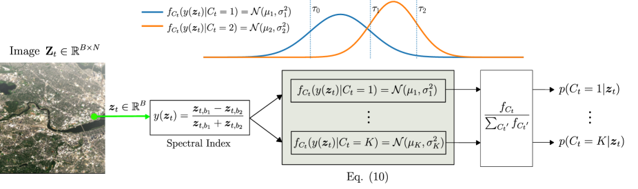
Figure 6: Overview of the proposed Spectral Index Classifier (SIC), where the values of standard broadband spectral indices such as the NDWI are converted into probabilities $p(C_{t}|\boldsymbol{z}_{t})$ as in Eq. (9). The proposed RBC framework can be applied on top of the SIC algorithm, which we refer to as recursive SIC (RSIC).

The length of intervals defining each class in the spectral index value $y(\boldsymbol{z}_{t})$ can be highly non-homogeneous and depends on the spectral index class thresholds $\tau_{i}$, being $i\in\{0,\ldots,K\}$. These thresholds define a hard classification result based on the spectral index value, with pixel $\boldsymbol{z}_{t}$ being assigned to the $i$-th class if and only if $y(\boldsymbol{z}_{t})\in(\tau_{i-1},\tau_{i}]$. Their length can be calculated as $L_{j}=\tau_{j}-\tau_{j-1}$, where $j\in\{1,\ldots,K\}$. The values of $\boldsymbol{\mu}$ and $\boldsymbol{\sigma}$ are calculated as $\mu_{j}=L_{j}/2+\tau_{j-1}$ and $\sigma_{j}=L_{j}/2$, so that the probability of a pixel belonging to a given class decreases smoothly as $y(\boldsymbol{z}_{t})$ moves away from the center of the interval and approaches one of the thresholds. The threshold values are determined empirically and are experiment-dependent, as discussed in Section 3.3.3.

3.3 Experimental setup

A classifier based on a GMM, an LR classifier, and the SIC algorithm introduced in Section 3.2, are compared to their recursive counterparts, namely the RGMM, RLR and RSIC algorithms. When working with data from test sites 1a, 1b, and 2, two additional pre-trained deep learning models are used as a benchmark in the context of water mapping: the DeepWaterMap (Isikdogan et al., 2017) and the WatNet (Luo et al., 2021) algorithms. All models under consideration are listed in Table 3. To ensure consistency when evaluating the RBC framework in different areas of study, we maintain the same number of classes across the three test sites, i.e., 2.

As discussed in the introduction, the instantaneous likelihood or class posterior to which the RBC framework is applied may be either semi-supervised, supervised or unsupervised. When the data model is unsupervised, the entire procedure may be viewed as unsupervised. The converse is also true for supervised methods. Considering this, when we describe the methodology followed in the training stage in Section 3.3.2, we are referring to the training stage of the GMM and LR models, as they need supervision.

3.3.1 Data splitting

A proportionally scaled timeline with the dates of images used for training and evaluation can be found in Fig. 7. Each downloaded image belongs to a different date and they are mostly spaced 5 days apart, i.e., the temporal resolution of Sentinel-2 satellites. However, temporal spacing between images may vary as a consequence of filtering images with high cloud/shadow cover and other discrepancies. On the one hand, large temporal spacings between training images translate into training data diversity. On the other hand, large temporal spacings between evaluation images can pose a challenge, because a change in land that occurs gradually can be interpreted as a sudden artifact to be discarded by the recursive algorithm. This matter is further discussed in Section 5.

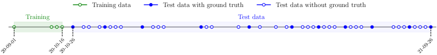
(a) Test sites 1a and 1b

(b) Test site 2

(c) Test site 3

Figure 7: Proportionally scaled timeline showing Sentinel-2 image dates used to train the GMM and LR models (green markers), and to test the GMM, LR, SIC, DWM and WN models, and their recursive counterparts (blue markers). The filled blue markers correspond to test images for which manually generated ground truth labels are available and used to evaluate the performance of the algorithms.

3.3.2 Training of the GMM and LR models

The LR and GMM models are trained in a weakly supervised approach. Training images correspond to those acquired on dates indicated with green markers in Fig. 7. To generate surrogate ground truth class labels, or pseudo-labels, the pixels from the training images are classified based on their spectral index value (MNDWI for test sites 1a, 1b and 2, and NDWI for test site 3) and considering the class thresholds $\boldsymbol{\tau}$ in Table 2. To obtain the generative model $p(z_{t}|C_{t})$ used in the RBGM from Eq. (3), one GMM is trained for each class label, i.e., $p(z_{t}|C_{t})$ is a GMM for each choice of $C_{t}$. To adequately represent the training pixels without overfitting, we select the smallest number of components for each GMM such that the histograms of the training data distribution and the one generated by the respective GMM are visually close.

3.3.3 Evaluation

Test images correspond to those acquired on dates indicated with blue markers in Fig. 7. Ground truth labels are generated for dates indicated with filled blue markers. Across all test sites, the dataset is imbalanced, with the majority of pixels being attributed to the land class in the two water mapping experiments and the forest class in the deforestation detection experiment. To prevent biases and ensure equal contribution from each class when benchmarking between models, balanced classification accuracy is used as a metric for the comparative analysis between instantaneous classifiers and their recursive counterparts in Section 4.1 and Section 4.2. In Section 4.3, the overall classification accuracy is used as a metric instead, as in this context the objective is not to benchmark between models but rather to assess the model sensitivity to determine a suitable value for the transition probability hyperparameter.

Ground truth: The lack of openly accessible labeled Sentinel-2 data for time-series analysis presents a significant challenge to the assessment of our framework. Consequently, water labels were manually generated for the dates employed in the quantitative analysis (filled blue markers in Fig. 7), and shared by the authors at (Calatrava et al., 2022). This procedure was facilitated by the LabelStudio tool . In the case of test site 3, the MultiEarth challenge dataset contains deforestation labels, which removes the need to manually generate ground truth labels for the third experiment. The dates for which deforestation labels are available do not necessarily match any date from the Sentinel-2 images in the MultiEarth dataset. Taking this into account, for each of the provided five labels, error classification maps are computed between the label and the classification result that is closest in time after the label date.

Parameter settings: The parameter values used for the conducted experiments are presented in Table 2. For the recursive algorithms, a trade-off between the robustness and adaptability is considered when tuning the hyperparameter $\epsilon$. Please refer to Section 4.3 for a better understanding of how this transition probability $\epsilon$ is selected. To convert a standard broadband spectral index into a probability as in Eq. (9), it is necessary to define the thresholds $\boldsymbol{\tau}$. These are tuned accordingly so that the generated classification maps obtained with the training images are visually close to the reference maps in Figs. 2,  3 and 5. As explained in Section 3.2, the thresholds are used to calculate $\boldsymbol{\mu}$ and $\boldsymbol{\sigma}$, which allows to evaluate the function $f_{C_{t}}\left(y(\boldsymbol{z}_{t})\right)$. The behavior of this function for the values used in the experiments is depicted in Fig. 8.

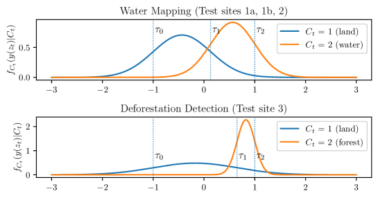
Figure 8: Functions $f_{C_{t}}\left(y(\boldsymbol{z}_{t})\right)$ introduced in Section 3.2. The corresponding values of $\boldsymbol{\tau}$, $\boldsymbol{\mu}$, $\boldsymbol{\sigma}$, and the spectral index $y(\boldsymbol{z}_{t})$ are the ones in Table 2 for the water mapping experiments (top subplot) and the deforestation detection experiment (bottom subplot).

Table 2: Parameter settings for the three experiments conducted in this research. The transition probability $\epsilon$ is defined in Section 3.1.3 and the regularization constant $\lambda$ is introduced in Section 3.1.4, Eq. (8). The thresholds $\boldsymbol{\tau}_{\mathrm{W}}$ and $\boldsymbol{\tau}_{\mathrm{D}}$ are used to generate surrogate ground truth labels to train the GMM and LR algorithms, as explained in Section 3.3.2, and to generate predictive probabilities of occurrence with the SIC algorithm (see Section 3.2).

Test sites 1a, 1b	$C_{t}\in\mathscr{C}_{\mathrm{W}}=\{\mathsf{land},\ \mathsf{water}\}$
	SIC	$\boldsymbol{\tau}_{\mathrm{W}}=[-1,\ 0.13,\ 1]$;
		$\boldsymbol{\mu}_{\mathrm{W}}=[-0.435,\ 0.565]$;
		$\boldsymbol{\sigma}_{\mathrm{W}}=[0.565,\ 0.435]$;
	$y_{\rm{MNDWI}}\left(\boldsymbol{z}_{t}\right)=\frac{z_{t,\rm{green}}-z_{t,\rm{SWIR}}}{z_{t,\rm{green}}+z_{t,\rm{SWIR}}}$
	RSIC	$\epsilon=0.05$; $\lambda=0$
	RGMM	$\epsilon=0.05$; $\lambda=0$
	RLR	$\epsilon=0.05$; $\lambda=0$
	RDWM, RWN	$\epsilon=0.05$; $\lambda=0.3$
Test site 2	$C_{t}\in\mathscr{C}_{\mathrm{W}}$
	SIC	$\boldsymbol{\tau}_{\mathrm{W}}$; $\boldsymbol{\mu}_{\mathrm{W}}$; $\boldsymbol{\sigma}_{\mathrm{W}}$
		$y_{\rm{MNDWI}}\left(\boldsymbol{z}_{t}\right)$
	RSIC	$\epsilon=0.01$; $\lambda=0$
	RGMM	$\epsilon=0.01$; $\lambda=0$
	RLR	$\epsilon=0.01$; $\lambda=0$
	RDWM, RWN	$\epsilon=0.01$; $\lambda=0.3$
Test site 3	$C_{t}\in\mathscr{C}_{\mathrm{D}}=\{\mathsf{land},\ \mathsf{forest}\}$
	SIC	$\boldsymbol{\tau}_{\mathrm{D}}=[-1,\ 0.65,\ 1]$;
		$\boldsymbol{\mu}_{\mathrm{D}}=[-0.175,\ 0.825]$;
	$\boldsymbol{\sigma}_{\mathrm{D}}=[0.825,\ 0.175]$
	$y_{\rm{NDWI}}\left(\boldsymbol{z}_{t}\right)=\frac{z_{t,\rm{green}}-z_{t,\rm{NIR}}}{z_{t,\rm{green}}+z_{t,\rm{NIR}}}$
	RSIC	$\epsilon=0.01$; $\lambda=0.1$
	RGMM	$\epsilon=0.05$; $\lambda=0.2$
	RLR	$\epsilon=0.05$; $\lambda=0.2$

4 Results

Complete results can be reproduced following the instructions in https://github.com/neu-spiral/RBC-SatImg. Overall, the RBC framework significantly increases the robustness of existing classification algorithms in multitemporal settings, while preserving the adaptability to changes in the land. Furthermore, it demonstrates substantial improvements when compared to pre-trained state-of-the-art deep learning-based classifiers, without the need for additional training data.

Table 3: Full name and abbreviation of the benchmark classification models, i.e., SIC (introduced in Section 3.2), GMM, LR, DWM (Isikdogan et al., 2017) and WN (Luo et al., 2021), and their recursive counterparts, i.e., RSIC, RGMM, RLR, RDWM and RWN, which derive from applying the proposed recursive Bayesian classification framework.

Full Name	Abbreviation
Spectral Index Classifier (Section 3.2)	SIC
Gaussian Mixture Model	GMM
Logistic Regression	LR
DeepWaterMap (Isikdogan et al., 2017)	DWM
WatNet (Luo et al., 2021)	WN
Recursive Spectral Index Classificatier	RSIC
Recursive Gaussian Mixture Model	RGMM
Recursive Logistic Regression	RLR
Recursive DeepWaterMap	RDWM
Recursive WatNet	RWN

4.1 Error classification maps

The following figures include the classification maps, error classification maps, and balanced classification accuracy results obtained using test images with available ground truth labels. RGB composite images of the studied areas are shown as a reference because they highlight changes in the scene. In the case of test site 1b, and due to space limitations, only one every two test images with ground truth data are included in the analysis. For classification map results encompassing all test images, including those without ground truth data, the interested reader may consult the supplemental material or refer to (Calatrava et al., 2023).

4.1.1 Test site 1

Water mapping results for test sites 1a and 1b are presented in Figs. 9 and 11, respectively. Additionally, Fig. 10 shows classification map results for test site 1b images with dates between 2021-07-08 and 2021-07-23 to illustrate a special event attributed to the reduction of water level. Fig. 9 shows noticeable differences among benchmark and recursive algorithms. For instance, the SIC algorithm classifies a large portion of the stream as land for dates 2021-05-19, 21-06-13, 2021-09-06 and 2021-09-26. The same is observed with the LR and DWM classifiers for dates 2021-05-19 and 2021-09-06. Nevertheless, their recursive counterparts, i.e., the RSIC, RLR and RDWM algorithms, can adequately classify most of the stream pixels as water. This translates into an increase in balanced classification accuracy of more than 20% provided by the use of recursion. The WN algorithm classifies some portions of land as water on dates between 2020-11-25 and 2021-07-08. While the RWN algorithm misclassifies part of the stream, it shows considerably more accurate classification maps. This can be specially observed for date 2021-04-09 and 2021-05-19, where WN misclassifies a large part of the land and the RBC offers an accuracy improvement of 7% and 5%, respectively. Overall, results suggest that the proposed RBC framework improves the performance of modern deep learning-based mapping algorithms. Moreover, it has been observed that the DWM and WN algorithms provide overconfident classification results, which can be an issue in recursive multitemporal classification. This is solved with the strategy proposed in Eq. (8) to regularize the predictive class posterior.

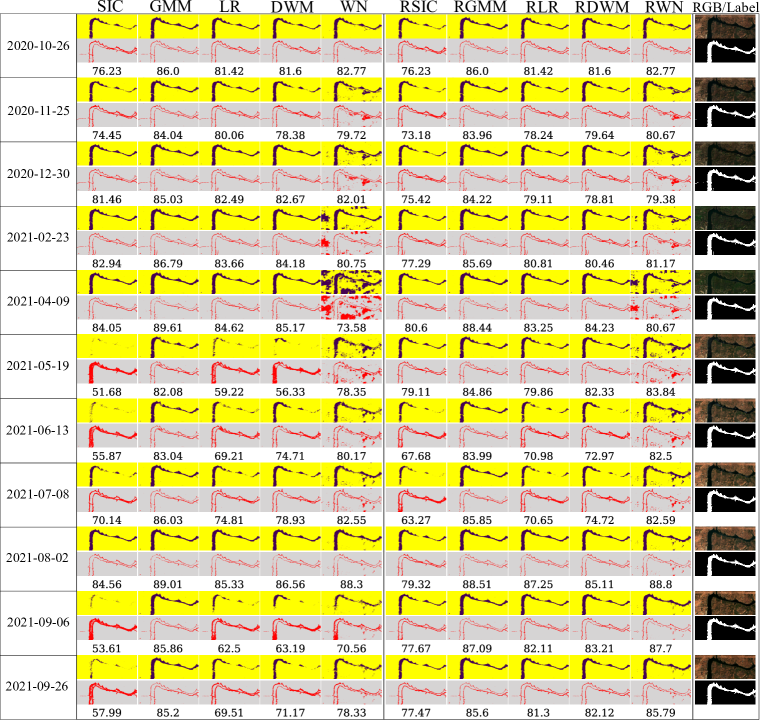
Figure 9: Water mapping results obtained for the Oroville dam downstream (test site 1a). Classification maps, error classification maps, and balanced classification accuracy results are presented. Purple and yellow represent water and land, respectively.

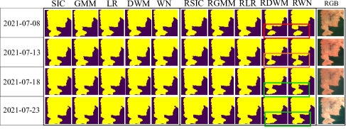
Figure 10: Classification map results obtained for the Oroville dam upstream (test site 1b) for dates between 2021-07-08 and 2021-07-23. The connection between the island at the bottom of the scene and the mainland poses a challenge to the RBC framework. Prioritizing robustness makes the recursive framework less flexible, potentially leading to the delayed detection of the union between the island and the mainland.

Results in Fig. 11 show that both the instantaneous classifiers and their recursive counterparts are able to adequately capture the decrease in water levels over time in the dam upstream in test site 1b. In the case of date 2020-12-30, the SIC, LR, DWM and WN algorithms misclassify a considerable amount of water as land, while their recursive counterparts output more correct classification maps. This results in an increase of balanced classification accuracy between 8% and 15% for these models. The RGMM is also able to recover some water pixels for this same date. However, this leads to a more modest improvement in balanced classification accuracy (under 3%), considering that the instantaneous classifier was already performing well. A similar effect is also observed on dates such as 2021-08-02, for which all methods provide adequate classification results and consequently the improvement introduced by recursion is moderate (under 5%). The trade-off between adaptability and robustness presents a challenge to the recursive framework for the upstream subscene of Oroville Dam. Prioritizing robustness makes the recursive framework less flexible, potentially leading to delayed detection of abrupt scene changes. For example, the increase in water level starting in February is better identified by the instantaneous classifiers, as they do not rely on information from previous images showing lower water levels. This results in a decrease in balanced classification accuracy of up to 6.5% when recursion is applied on the date 2021-04-09. However, this setback is gradually resolved on subsequent dates, as indicated by improved classification results on 2021-06-13. Another example is the connection between the island at the bottom of the scene and the mainland. This event goes undetected by the recursive versions of the DWM and WN algorithms on 2021-07-08. Nevertheless, it is successfully identified in the subsequent evaluation on 2021-07-13. This phenomenon is shown with the obtained classification maps in Fig. 10. The introduction of the normalization constant in Eq. (8) aims to counteract the overconfidence of the deep learning-based classifiers. However, this leads these models to rely more on data from past time instances, enhancing their robustness but constraining their adaptability.

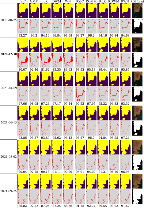
Figure 11: Water mapping results obtained for the Oroville dam upstream (test site 1b). Classification maps, error classification maps, and balanced classification accuracy results are presented. Purple and yellow represent water and land, respectively.

4.1.2 Test site 2

Water mapping results for test site 2 are presented in Fig. 12. The interested reader may refer to Appendix A, where classification map results are shown for a three-class classification experiment with the same data, thus demonstrating the scalability of the framework to handle more complex classification tasks. Test site 2 extends over an area covering the Boston harbor, the Charles river lower, mid and some upper basins, and the Mystic river lower basin. Since most of these correspond to urban and suburban areas, we can find many reflective surfaces from, e.g., building terraces and metal sheds, which lead to pixels with high spectral reflectance. Such pixels may be easily misclassified by water since their MNDWI values are close to zero. This can be observed in the classification maps from 2020-12-13, where the recursive algorithms result in fewer misclassifications of reflective surface pixels as water. However, due to class imbalance, this reduction in misclassifications does not necessarily translate to a performance increase in terms of balanced classification accuracy. Specifically, on this date, the DWM model misclassifies a total of 49,264 land pixels, while the RDWM model misclassifies 8,341 land pixels. Although the latter is significantly lower, concerning the water class, the RDWM misclassifies 19,734 pixels compared to 10,738 misclassifications by the DWM model, which then achieves a balanced classification result 1% higher than the RDWM. On 2021-05-27, given the appearance of cyanobacterial blooms, due to which the water becomes diluted with chlorophyll pigments, an important portion of water pixels are classified as land by the instantaneous classifiers, whereas their recursive versions provide more accurate classification maps. This leads to an improvement in balanced classification accuracy of around 7% for the LR classifier and of 10% for the rest of the recursive models. The WN algorithm exhibits poor performance, particularly since 2021-05-27, misclassifying a significant portion of land pixels as water. As a result, we observe an increase in balanced classification accuracy of more than 10% on 2021-05-27 and 2021-07-31, and a 7.5% rise on 2021-09-14. Overall, the recursive algorithms provide significantly more robust performance than their non-recursive counterparts. The latter are less sensitive to atmospheric interference and illumination factors. For some dates, the recursion introduces a smoothing effect, which makes it more difficult to adapt to class changes. This can be understood by comparing the classification maps obtained with the SIC and RSIC algorithms on 2021-04-24.

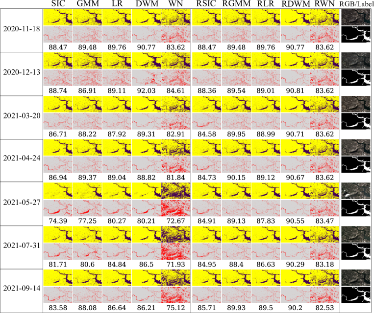
Figure 12: Water mapping results obtained for the Charles river basin (test site 2). Classification maps, error classification maps, and balanced classification accuracy results are presented. Purple and yellow represent water and land, respectively.

4.1.3 Test site 3

Deforestation detection results for test site 3 are illustrated in Fig. 13. On dates 2020-06-10, 2020-08-04, and 2021-05-26, cloud presence disrupts the performance of the instantaneous classifiers, while their recursive counterparts demonstrate adequate classification map results. This led to a rise in balanced classification accuracy of 5%, 7.5%, and 9% from the RSIC, RGMM, and RLR algorithms on 2020-06-10, and 12%, 8%, and 12.5% on 2021-05-26. On 2020-08-04, despite improved classification maps, there was a slight enhancement in balanced classification accuracy without the use of recursion. We attribute this to the class imbalance in the dataset, where the forested area substantially exceeds the deforested area. The adaptability of the framework is evident in the classification map results from 2021-05-26, which reveal a newly deforested area detected by the three recursive algorithms but missed by their non-recursive counterparts. On the subsequent date (2021-08-19), only the RSIC algorithm can detect this same deforested area, which remains undetected for the other algorithms. This failure of the RGMM and RLR algorithms is due to repeated failures in the task by the instantaneous classifiers, which disrupts the performance of their recursive counterparts. Supplemental results show that the recursive classifiers need two iterations where the instantaneous classifiers detect the deforested area to acknowledge this change, as a consequence of the trade-off between the robustness and adaptability of the framework.

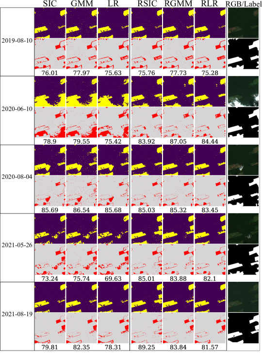
Figure 13: Deforestation detection results obtained for the Amazon rainforest area (test site 3). Classification maps, error classification maps, and balanced classification accuracy results are presented. Purple and yellow represent forest and deforested area, respectively. For this experiment, Sentinel-2 images and deforestation labels have been obtained from the MultiEarth challenge dataset (Cha et al., 2023).

4.2 Classification accuracy visualization

The boxplot in Fig. 14 shows the distribution of the balanced classification accuracy results presented in the previous subsection. The introduction of recursion mitigates negative outliers from the non-recursive models. Additionally, negative outliers from the recursive models fall within the interquartile range of the non-recursive models. For instance, when analyzing the RSIC model with test site 1a data, there is a significant reduction in result variability, with two negative outliers falling within the interquartile range of the SIC model. A noticeable trend is the reduced variability in performance among the recursive algorithms, evident from the narrower spread of balanced accuracy values. This is evident when applying the RBC framework to the DWM and WN deep learning models with test site 2 data. While the upper limits remain consistent and do not show a significant increase, the lower range of results for the recursive models is notably higher. This suggests that although peak accuracies do not exhibit a significant rise, there is a marked enhancement in the lower-end performance, implying a more consistent and improved overall performance across the tested algorithms, which results from the robustness provided by the RBC framework.

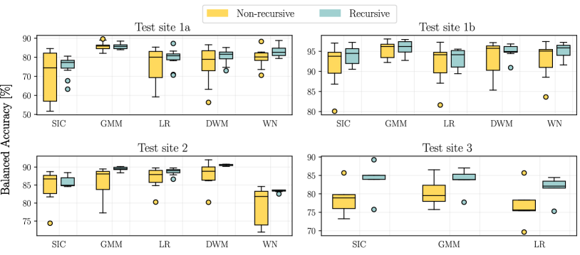
Figure 14: Boxplot showing the distribution of balanced accuracy results for the SIC, GMM, LR, DWM and WN algorithms (yellow boxes), including their recursive counterparts (blue boxes). The boxplot illustrates the median with a line within each box, the interquartile range with the box boundaries, and the data range with whiskers. Outliers are represented as filled individual circles.

4.3 Sensitivity analysis

The class transition probabilities, denoted as $\epsilon$ and introduced in Section 3.1.3, are site-specific, emphasizing the need for careful selection of their values. In this section, we present an analysis of the model sensitivity to this hyperparameter. In Fig. 15, a study on the sensitivity of the water mapping model is conducted using images from the upstream Oroville dam site in test site 1b. Variations in the number of pixels classified as water are depicted under varying $\epsilon$ values ranging from 0.1 to 0.8 for the RSIC, RGMM, and RLR models. Additionally, results are presented for their non-recursive counterparts in grey color. Despite the 5-day temporal resolution of Sentinel-2 images, the x-axis displays varying temporal gaps due to the filtering of cloud-covered data. Results from dates 2020-11-10, 2020-12-30, and 2021-01-19 indicate that the discriminative recursive models (RLR and RSIC) show higher sensitivity to changes in the transition probabilities compared to the RGMM model. Notably, the number of water pixels exhibits more abrupt variations for different $\epsilon$ values with the RSIC model, especially evident for $\epsilon=0.8$, where the count decreases from approximately 7000 to 3500 between 2020-12-10 and 2020-12-30. Conversely, for the same model with $\epsilon=0.1$, this variation remains under 1000 pixels. The RLR model displays a similar behavior for these dates, while the RGMM model demonstrates comparatively smaller variations in the number of water pixels.

Sensitivity is best assessed on dates with considerable changes in class distribution, such as those resulting from natural phenomena like draining before extreme rainfall. The varying temporal gaps between dates also impact class distribution. Larger $\epsilon$ values cause the RSIC and RLR models to fail during such events. For RLR, a small value of $\epsilon=0.1$ appears to smooth abrupt changes in the prediction of water pixels. Similarly, RSIC presents smoother results for $\epsilon=0.1$ compared to higher $\epsilon$ values. The RGMM model appears less sensitive to changes in the transition probability hyperparameter, displaying relatively similar amounts of water pixels across all dates for different $\epsilon$ values. However, an abrupt change in the number of water pixels is observed for the highest $\epsilon=0.8$ value on 2020-08-27. As a sanity check, we confirm that results match between the instantaneous classifier (grey color) and its recursive version for $\epsilon=0.5$ (lime green color), as RBC framework is equivalent to the likelihood when $\epsilon=0.5$. Considering these results, we decided to set $\epsilon$ to a small value for the two water mapping experiments, as specified in Table 2.

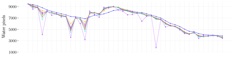
(a) RSIC

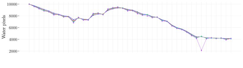
(b) RGMM

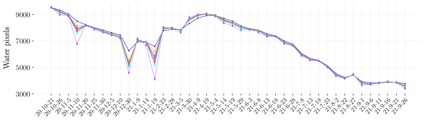
(c) RLR

Figure 15: Sensitivity analysis of the RSIC, RGMM and RLR models conducted with images of the Oroville dam upstream (test site 1b), in the context of water mapping. The number of pixels classified as water is compared between realizations of the water mapping experiment for $\epsilon$ values between 0.1 and 0.8.

A sensitivity analysis is performed using data from test site 3 to determine the optimal hyperparameter value for the deforestation detection experiment. The results in Fig. 16 show the overall classification accuracy concerning different $\epsilon$ values. As in the previous experiment, for $\epsilon=0.5$, we obtain the equivalent to a non-recursive classifier, i.e., time-invariant. For values above $\epsilon=0.5$, the recursive algorithms demonstrate inferior performance compared to their non-recursive counterparts. An $\epsilon>0.5$ suggests a higher likelihood for a pixel to transition between classes rather than remaining in the same class, which is an unrealistic hypothesis. The left subplot part highlighted with a light grey background and further magnified in the right subplot, shows that the highest classification accuracy is achieved for $0<\epsilon<0.1$. The optimal $\epsilon$ values yielding the best results are 0.01, 0.04, and 0.045 for the RSIC, RGMM, and RLR algorithms, respectively. Consequently, we have chosen to set $\epsilon$ values to 0.01, 0.05, and 0.05 for the RSIC, RGMM, and RLR algorithms, respectively, in the deforestation detection experiment (see Table 2) The RGMM and RLR algorithms show a wider range of $\epsilon$ values providing classification accuracy results near the best accuracy, as opposed to the RSIC algorithm, which shows greater sensitivity to $\epsilon$ variations.

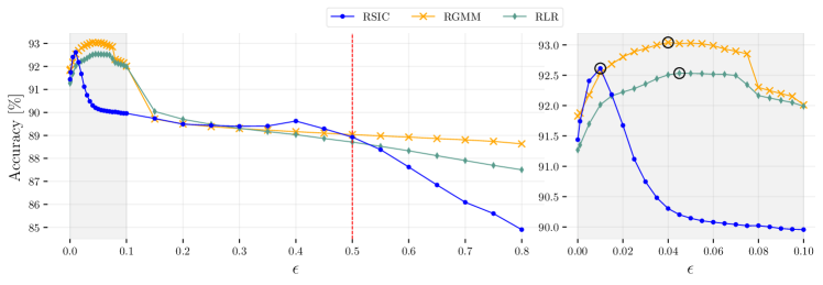
Figure 16: Sensitivity analysis of the RSIC, RGMM and RLR models conducted with test site 3 data, in the context of deforestation detection. Average overall classification accuracy results are presented for $\epsilon$ values between 0 and 0.8.

5 Discussion

The implications of the main findings of this research are presented hereafter. In this paper, we propose a recursive Bayesian classification method for robust multitemporal image classification that can be built on top of time-independent generative or discriminative models. The recursive characteristic of the method makes it more robust to common variations found in remote sensing imagery such as illumination and atmospheric interference, e.g., different aerosol concentrations or viewing angles. The proposed method is simple, easy to use, interpretable, and controlled by a unique explainable hyperparameter $\epsilon$ representing the probability of transitioning among the different classification labels. As a consequence, $\epsilon$ governs the trade-off between adaptability to natural changes in scene and robustness to outliers caused by illumination of atmospheric interferences. As the class transition probability is specific to each site and the instantaneous classification algorithm, a study has been performed on the model sensitivity to the hyperparameter $\epsilon$ in the context of water mapping and deforestation detection. The sensitivity analysis in Section 4.3 shows that to obtain robust classification results, i.e., that are insensitive to undesired abrupt changes in the image, it is best to select small values of $\epsilon$ for scenes that are expected to change smoothly.

In this work, we demonstrated the proposed methodology by leveraging different models such as GMMs, LR, deep learning-based models, and the introduced SIC classifier. As a key contribution, we provide a clear framework to convert classifiers based on spectral indices, such as the NDVI, NDWI and MNDWI, into robust multitemporal classifiers. Spectral indices are a valued tool in the remote sensing community given their simplicity and low required computational cost. However, they are highly sensitive to changes in illumination and pixel disturbances, which are commonly present in remotely sensed imagery. The proposed SIC classifier allows to convert spectral index values into a probability measure with the mapping presented in Eq. (9). Furthermore, the proposed recursive approach can be easily applied to more sophisticated methodologies such as pre-trained deep learning-based classifiers without requiring additional training data. Models like deep neural networks are very flexible and can lead to overconfident classification results, thus diminishing the impact that information from previous time instants has on the model and reducing the robustness of the algorithm. To circumvent this phenomenon, we proposed to empirically reduce such overconfidence by inserting a positive constant to slightly push the probabilities towards a discrete uniform distribution as in Eq. (8).

5.1 RBC framework limitations and challenges

Regarding the limitations of this work, we highlight the scarcity of ground truth multitemporal classification maps. The scarcity of ground truth poses challenges in conducting a quantitative assessment of the results. For the assessment with data from test sites 1a, 1b and 2, water labels were manually generated using the LabelStudio tool by the authors. Additionally, classification map results for a three-class classification task with test site 2 data can be referred to in Appendix A, which shows that the RBC framework may be successfully scaled to more complex classification tasks. Quantitative analysis was facilitated by the availability of open-source labeled deforestation data in the MultiEarth challenge dataset (Cha et al., 2023), which complemented the visual inspection of classification maps obtained from test site 3. However, this dataset does not provide deforestation labels for each acquisition date, as explained in Section 3.3.1, and consequently, quantitative metrics could only be computed for a limited portion of the time-series. Specifically, error classification maps were computed for only 5 images, whose dates are marked with filled blue markers in Fig. 7. Furthermore, temporal misalignment between image and label dates in the MultiEarth dataset required comparing each label to the classification result closest in time after its date, which reduces the reliability of the evaluation of the classification results due to the temporal gaps. Overall, the assessment of the proposed technique benefits from a combined approach, integrating both quantitative metrics and visual inspection of obtained results for a comprehensive understanding of its advantages.

Another challenge arises due to the need to remove a considerable number of images from the time-series given the frequent occurrence of effects such as clouds. In the data pre-processing stage and for the data in test site 3, from the available 225 images, 182 images are discarded given their high cloud and cloud shadow percentages according to the CI₂ and CSI indices (Zhai et al., 2018). Also, 12 images are filtered out by visual inspection. The frequent appearance of clouds and other atmospheric disturbances poses an important limitation in the application of this technique because part of the dataset imagery required for accurate analysis is obstructed. This becomes more evident when recursion takes place, as large temporal spacing between evaluation images might result in gradual changes in land being mistaken by sudden artifacts to be discarded.

Our choice for constant transition probabilities leads to a methodology that has a low associated computational cost, can be used over large geographic areas, and is easier to tune. However, this could come at the expense of fidelity to real-world dynamics, as natural systems and human activities often undergo changes that affect transition dynamics. Recursion may be leveraged to automatically determine the class transition probabilities over the time-series. The same could be done with the class prior probabilities. Another significant limitation of our work is the non-exploitation of spatial correlations between pixels. We explicitly assumed the labels from different pixels to be independent, thus, the RBC framework does not leverage spatial structures and patterns that are present in nature.

Overall, promising results have been obtained within the context of water mapping with test sites 1a, 1b and 2, deforestation detection with test site 3 and land cover mapping with the additional experiment in Appendix A. The proposed recursive models are robust to changes in the illumination level of the scene, as opposed to their non-recursive counterparts. This robustness is strongly observed when images include pixel disturbances or undesired changes in illumination, which hurt the non-recursive models but can be successfully overcome for most dates when the proposed recursive framework is applied. Also, it is important to ensure the adaptability of the recursive methods so that they can identify natural phenomena and incorporate smooth changes in the image time-series.

6 Conclusion

In this paper, we introduced a recursive Bayesian classification framework for satellite image time-series that improves the decision-making process in land cover classification algorithms by leveraging previous classification results. The study conducted three two-class experiments using Sentinel-2 data: water mapping of an embankment dam in Oroville, California, USA; water mapping of the Charles River Basin in Boston, Massachusetts, USA; and deforestation detection in the Amazon Rainforest. The Spectral Index Classification (SIC) classifier was introduced to predict probabilities of occurrence for land and water pixels based on standard spectral indices. We compared the performance of three different instantaneous classifiers and their recursive counterparts (GMM, LR, and SIC) and also benchmarked against two pre-trained deep learning classifiers (DeepWaterMap and WatNet algorithms) in water mapping experiments. Results indicated that the proposed framework notably increases the robustness against outliers of existing classifiers in a multitemporal setting, even when applied to deep learning-based models, without the need for additional training data. This improvement comes with low computational costs and minimal supervision, distinguishing it from other recursive approaches that typically require substantial training data. Future work will investigate the incorporation of spatial information into the recursive Bayesian classification strategy to improve the robustness against non-informative spectral variations, as well as a method to automatically determine the class transition probabilities and their prior probabilities.

Declaration of Competing Interest

The authors of this paper declare that they have no known personal relationships or competing financial interests that could have appeared to influence this research.

Dataset and supplemental results

A Python implementation of the proposed algorithms can be found at https://github.com/neu-spiral/RBC-SatImg, with the pre-processed data and manually generated ground truth labels being available at (Calatrava et al., 2022). Supplemental material containing additional experimental results is also available with this paper.

Appendix A Land cover classification experiment

Land cover classification results for test site 2 are presented in Fig. 17. Performance evaluation in this experiment is restricted to the visual inspection of the classification maps given the lack of ground truth data for the vegetation class in this test site. Results suggest that seasonal variations in the distribution of land, water and vegetation are captured well by the instantaneous classifiers and their recursive counterparts. The decrease in the amount of vegetation starting from November (through winter) with an increase in dry land (at dates 2020-12-13 and 2021-03-20) is represented by an increase in yellow pixels until May, followed by an increase in the number of vegetation pixels through summer and fall (from 2021-05-27 to 2021-09-14). The advantages of the RBC framework are evident, especially on the date 2020-12-13, where the instantaneous classifiers misclassify a substantial land area as water, while the recursive algorithms properly identify the land pixels. On 2021-09-14, both the SIC and LR algorithms fail to identify a section of the water body, yet their recursive counterparts successfully handle this task.

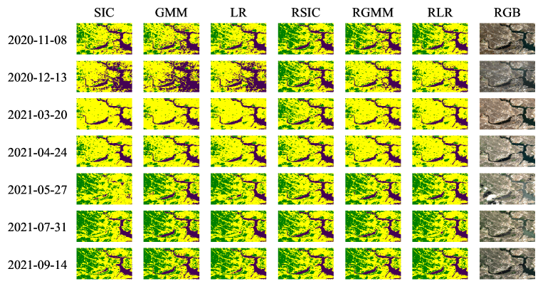
Figure 17: Land cover classification results obtained for the Charles river basin area covered by test site 2. Purple, green and yellow represent water, vegetation and land, respectively. Images are arranged in chronological order. By visually inspecting these results, it can be assessed that the proposed RBC framework provides adaptability to seasonal changes and robustness to highly reflective surfaces and other disturbances.

Table 4: Parameter settings for the three-class land cover classification experiment with test site 2 data.

Test site 2	$C_{t}\in\mathscr{C}_{\mathrm{LC}}=\{\mathsf{water},\ \mathsf{land},\ \mathsf{vegetation}\}$
	SIC	$\boldsymbol{\tau}_{\mathrm{LC}}=[-1,\ -0.05,\ 0.35,\ 1]$;
		$\boldsymbol{\mu}_{\mathrm{LC}}=[-0.525,\ 0.149,\ 0.675]$;
		$\boldsymbol{\sigma}_{\mathrm{LC}}=[0.475,\ 0.19,\ 0.325]$;
	$y_{\rm{NDVI}}\left(\boldsymbol{z}_{t}\right)=\frac{z_{t,\rm{NIR}}-z_{t,\rm{red}}}{z_{t,\rm{NIR}}+z_{t,\rm{red}}}$
	RSIC	$\epsilon=0.05$; $\lambda=0$
	RGMM	$\epsilon=0.05$; $\lambda=0$
	RLR	$\epsilon=0.05$; $\lambda=0$

Supplemental Results

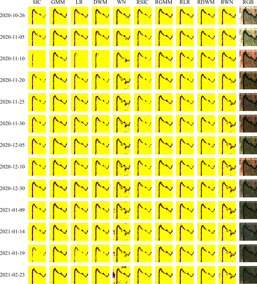
Figure 18: Supplemental results from test site 1a including classification maps for all dates (from 2020-10-26 to 2021-02-23).

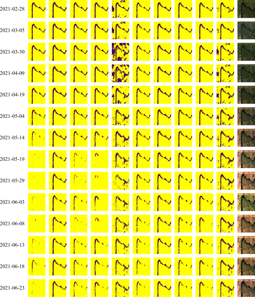
Figure 19: Supplemental results from test site 1a including classification maps for all dates (from 2021-02-28 to 2021-06-23).

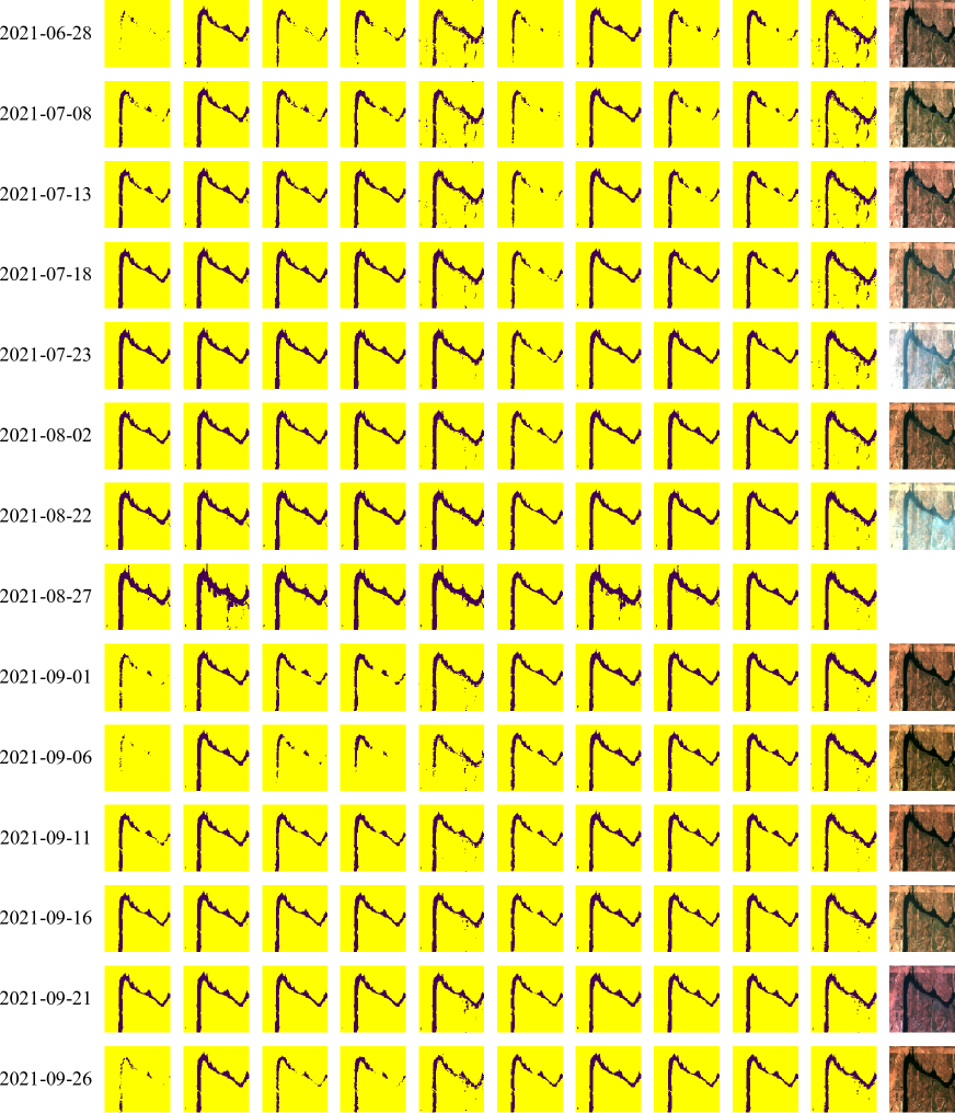
Figure 20: Supplemental results from from test site 1a including classification maps for all dates (from 2021-06-28 to 2021-09-26).

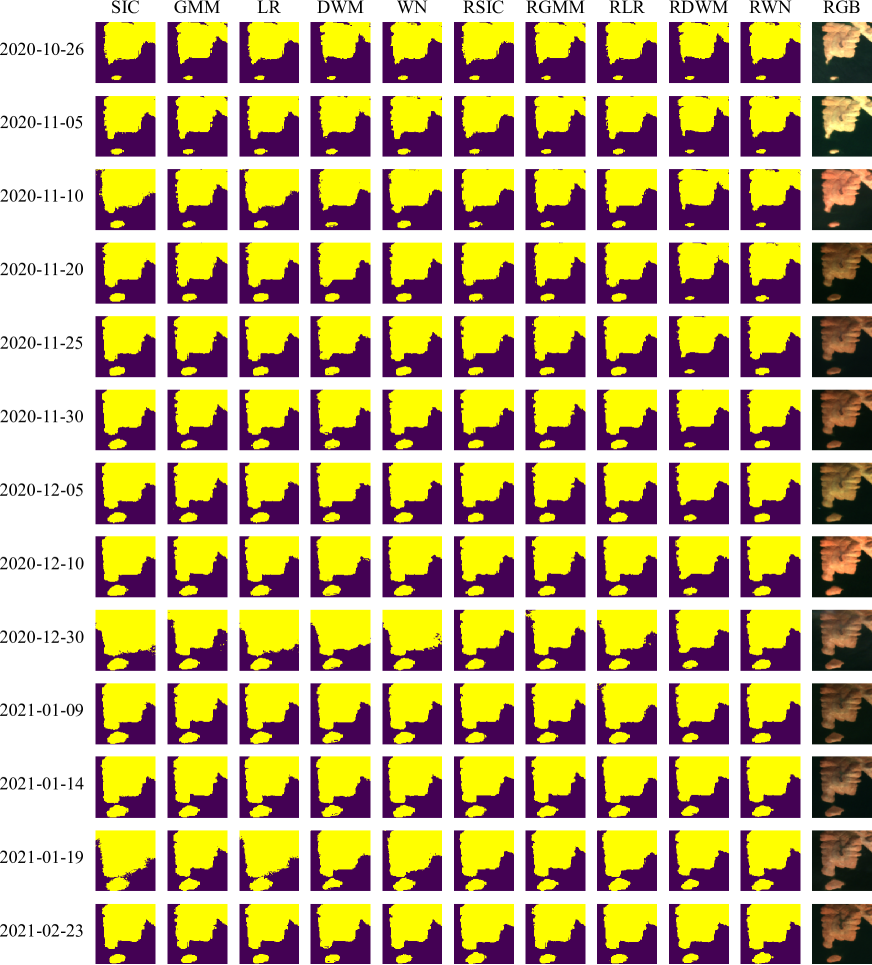
Figure 21: Supplemental results from test site 1b including classification maps for all dates (from 2020-10-26 to 2021-02-23).

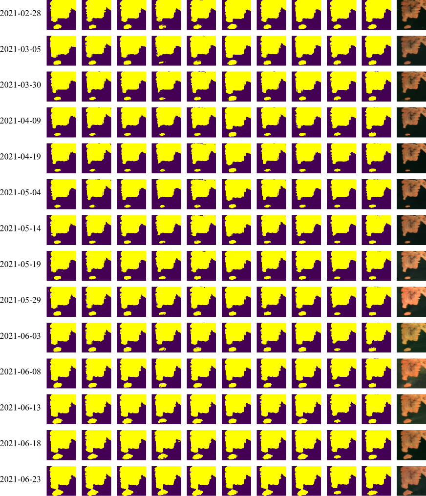
Figure 22: Supplemental results from test site 1b including classification maps for all dates (from 2021-02-28 to 2021-06-23).

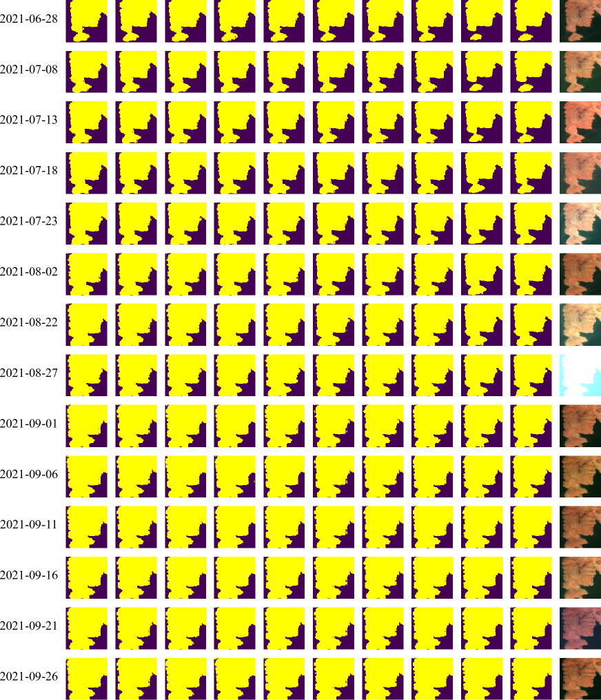
Figure 23: Supplemental results from test site 1b including classification maps for all dates (from 2021-06-28 to 2021-09-26).

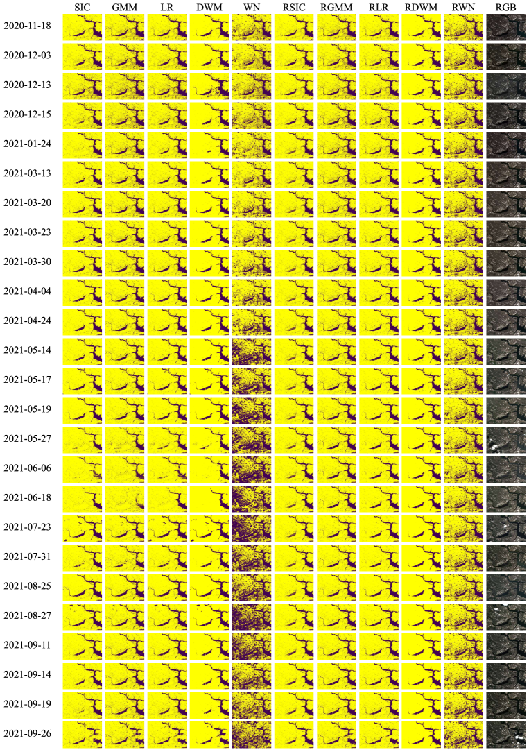
Figure 24: Supplemental results from test site 2 including classification maps for all dates (from 2020-11-18 to 2021-09-26).

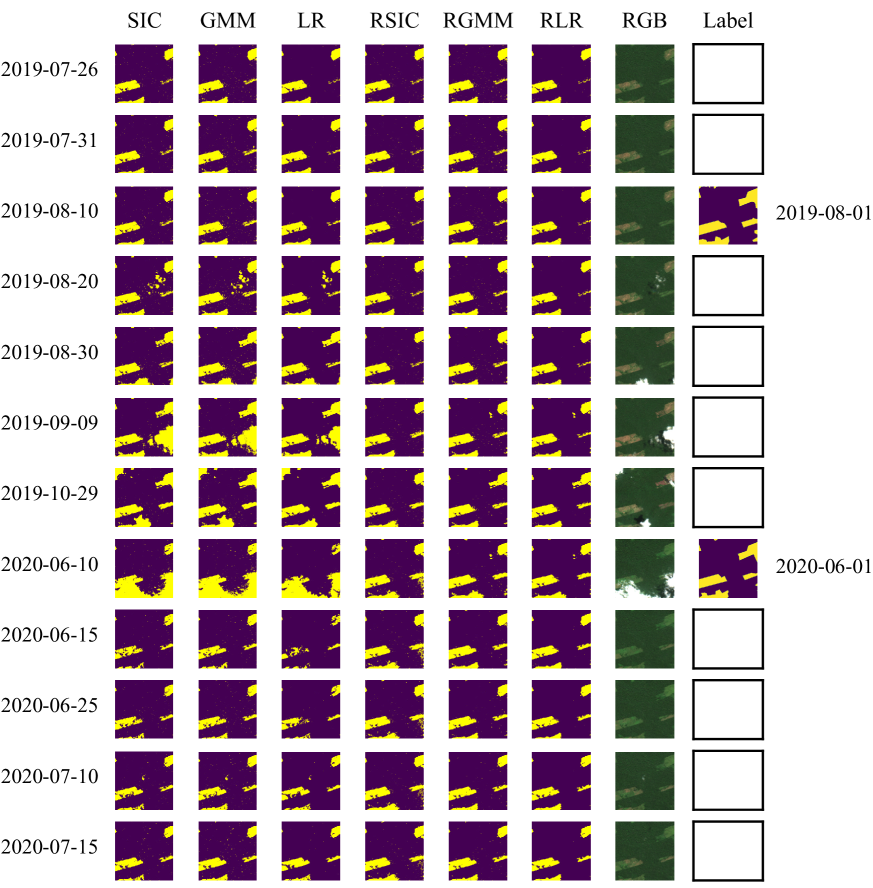
Figure 25: Supplemental results from test site 3 including classification maps for all dates (from 2019-07-26 to 2020-07-15). Deforestation label dates are shown in the last column.

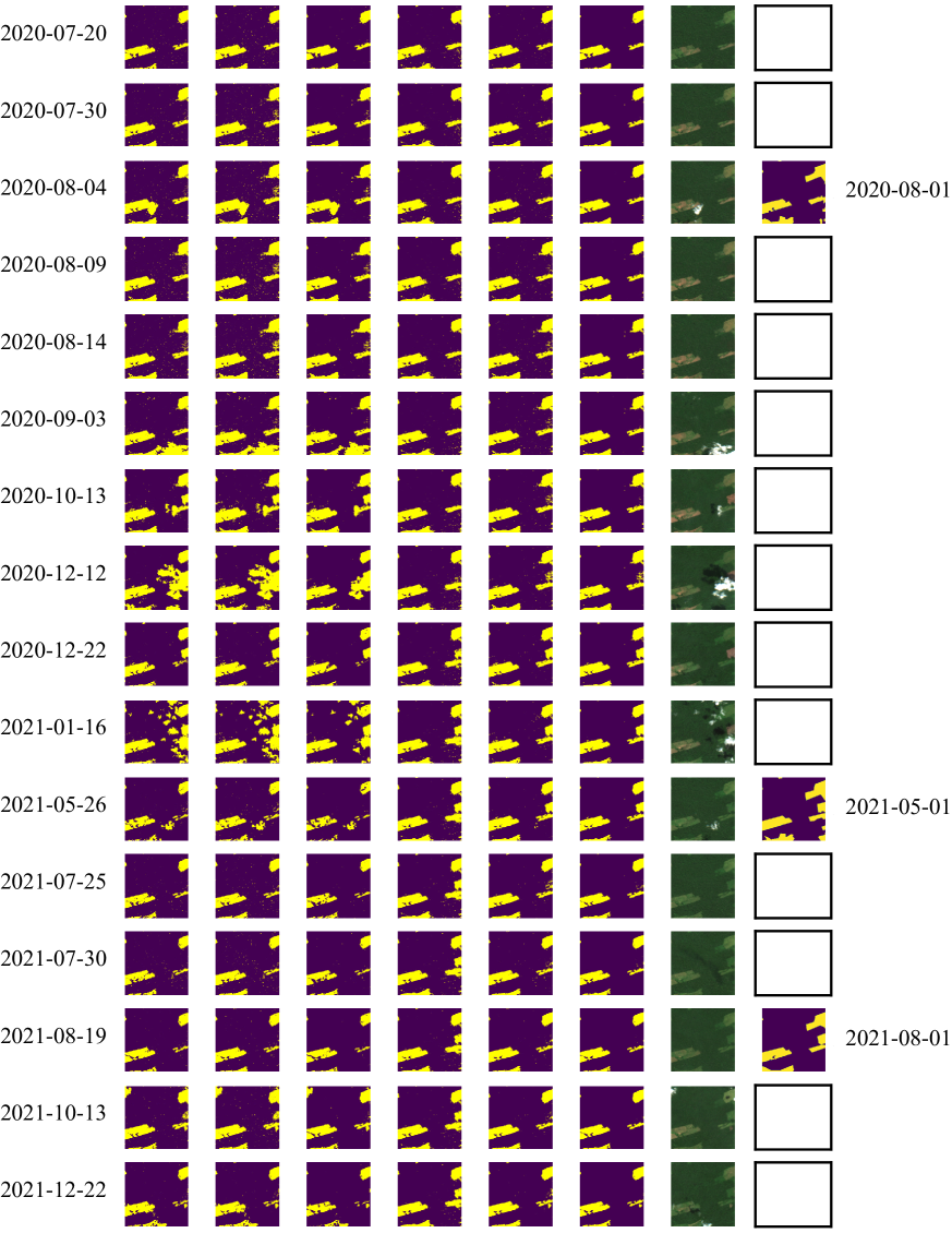
Figure 26: Supplemental results from test site 3 including classification maps for all dates (from 2020-07-20 to 2021-12-22). Deforestation label dates are shown in the last column.

References

- Acharya et al. (2018) Acharya, T., Subedi, A., Lee, D., 2018. Evaluation of Water Indices for Surface Water Extraction in a Landsat 8 Scene of Nepal. Sensors 18, 2580. doi:10.3390/s18082580.
- Anderson (1976) Anderson, J.R., 1976. A land use and land cover classification system for use with remote sensor data. volume 964. US Government Printing Office.
- Barber (2011) Barber, D., 2011. Bayesian Reasoning and Machine Learning. 04-2011 ed., Cambridge University Press. URL: http://www.cs.ucl.ac.uk/staff/d.barber/brml. in press.
- Borsoi et al. (2021a) Borsoi, R.A., Imbiriba, T., Bermudez, J.C.M., Richard, C., 2021a. Fast Unmixing and Change Detection in Multitemporal Hyperspectral Data. IEEE Transactions on Computational Imaging 7, 975–988.
- Borsoi et al. (2021b) Borsoi, R.A., Imbiriba, T., Bermudez, J.C.M., Richard, C., Chanussot, J., Drumetz, L., Tourneret, J.Y., Zare, A., Jutten, C., 2021b. Spectral Variability in Hyperspectral Data Unmixing: A Comprehensive Review. IEEE Geoscience and Remote Sensing Magazine 9, 223–270.
- Borsoi et al. (2020) Borsoi, R.A., Imbiriba, T., Closas, P., Bermudez, J.C.M., Richard, C., 2020. Kalman filtering and expectation maximization for multitemporal spectral unmixing. IEEE Geoscience and Remote Sensing Letters 19, 1–5.
- Calatrava et al. (2022) Calatrava, H., Duvvuri, B., Li, H., Borsoi, R., Imbiriba, T., Beighley, E., Erdogmus, D., Closas, P., 2022. Sentinel-2 Images from Oroville Dam and Charles River. URL: https://doi.org/10.5281/zenodo.7391412, doi:10.5281/zenodo.7391412.
- Calatrava et al. (2023) Calatrava, H., Duvvuri, B., Li, H., Borsoi, R., Imbiriba, T., Beighley, E., Erdoğmuş, D., Closas, P., 2023. Recursive classification of satellite imaging time-series: An application to land cover mapping. arXiv preprints URL: https://arxiv.org/abs/2301.01796.
- Campbell et al. (2021) Campbell, A., Shi, Y., Rainforth, T., Doucet, A., 2021. Online variational filtering and parameter learning, in: Beygelzimer, A., Dauphin, Y., Liang, P., Vaughan, J.W. (Eds.), Advances in Neural Information Processing Systems. URL: https://openreview.net/forum?id=et2st4Jqhc.
- Cha et al. (2023) Cha, M., Angelides, G., Hamilton, M., Soszynski, A., Swenson, B., Maidel, N., Isola, P., Perron, T., Freeman, B., 2023. Multiearth 2023 – multimodal learning for earth and environment workshop and challenge. arXiv:2306.04738.
- Chouteau et al. (2022) Chouteau, F., Gabet, L., Fraisse, R., Bonfort, T., Harnoufi, B., Greiner, V., Le Goff, M., Ortner, M., Paveau, V., 2022. Joint Super-Resolution and Image Restoration for PLÉIADES NEO Imagery. ISPRS - International Archives of the Photogrammetry, Remote Sensing and Spatial Information Sciences 43B1, 9–15. doi:10.5194/isprs-archives-XLIII-B1-2022-9-2022.
- Closas et al. (2009) Closas, P., Fernandez-Prades, C., Fernandez-Rubio, J.A., 2009. A bayesian approach to multipath mitigation in gnss receivers. IEEE Journal of Selected Topics in Signal Processing 3, 695–706. doi:10.1109/JSTSP.2009.2023831.
- Cohen and Berdugo (2002) Cohen, I., Berdugo, B., 2002. Noise estimation by minima controlled recursive averaging for robust speech enhancement. Signal Processing Letters, IEEE 9, 12 – 15. doi:10.1109/97.988717.
- Constantin et al. (2022) Constantin, A., Fauvel, M., Girard, S., 2022. Joint Supervised Classification and Reconstruction of Irregularly Sampled Satellite Image Times Series. IEEE Transactions on Geoscience and Remote Sensing 60. doi:10.1109/TGRS.2021.3076667.
- Demir et al. (2013) Demir, B., Bovolo, F., Bruzzone, L., 2013. Classification of time series of multispectral images with limited training data. IEEE Transactions on Image Processing 22, 3219–3233.
- Demirkaya et al. (2021) Demirkaya, A., Imbiriba, T., Lockwood, K., Rampersad, S., Alhajjar, E., Guidoboni, G., Danziger, Z., Erdoğmuş, D., 2021. Cubature kalman filter based training of hybrid differential equation recurrent neural network physiological dynamic models, in: 2021 43rd Annual International Conference of the IEEE Engineering in Medicine & Biology Society (EMBC), IEEE. pp. 763–766.
- Deng et al. (2019) Deng, Z., Zhu, X., He, Q., Tang, L., 2019. Land use/land cover classification using time series Landsat 8 images in a heavily urbanized area. Advances in Space Research 63. doi:10.1016/j.asr.2018.12.005.
- Ekercin (2007) Ekercin, S., 2007. Coastline Change Assessment at the Aegean Sea Coasts in Turkey Using Multitemporal Landsat Imagery. Journal of Coastal Research - J COASTAL RES 23, 691–698. doi:10.2112/04-0398.1.
- Fang et al. (2021) Fang, Z., Wang, Y., Peng, L., Hong, H., 2021. Predicting flood susceptibility using LSTM neural networks. Journal of Hydrology 594. doi:10.1016/j.jhydrol.2020.125734.
- Farhadi et al. (2022) Farhadi, H., Esmaeily, A., Najafzadeh, M., 2022. Flood monitoring by integration of Remote Sensing technique and Multi-Criteria Decision Making method. Computers and Geosciences 160, 105045. URL: https://www.sciencedirect.com/science/article/pii/S0098300422000127, doi:https://doi.org/10.1016/j.cageo.2022.105045.
- Frazier and Page (2000) Frazier, P., Page, K., 2000. Water Body Detection and Delineation with Landsat TM Data. Photogrammetric Engineering and Remote Sensing 66, 1461–1467.
- Gadrani et al. (2018) Gadrani, L., Lominadze, G., Tsitsagi, M., 2018. F assessment of landuse/landcover (LULC) change of Tbilisi and surrounding area using remote sensing (RS) and GIS. Annals of Agrarian Science 16, 163–169. URL: https://www.sciencedirect.com/science/article/pii/S1512188718300824, doi:https://doi.org/10.1016/j.aasci.2018.02.005.
- Gao et al. (2016) Gao, H., Wang, L., Jing, L., Xu, J., 2016. An effective modified water extraction method for Landsat-8 OLI imagery of mountainous plateau regions. IOP Conference Series: Earth and Environmental Science 34, 012010. doi:10.1088/1755-1315/34/1/012010.
- Gómez et al. (2016) Gómez, C., White, J.C., Wulder, M.A., 2016. Optical remotely sensed time series data for land cover classification: A review. ISPRS Journal of Photogrammetry and Remote Sensing 116, 55–72.
- Griffiths et al. (2019) Griffiths, P., Nendel, C., Hostert, P., 2019. Intra-annual reflectance composites from Sentinel-2 and Landsat for national-scale crop and land cover mapping. Remote sensing of environment 220, 135–151.
- Gujjar and Vaughan (2019) Gujjar, P., Vaughan, R., 2019. Classifying pedestrian actions in advance using predicted video of urban driving scenes, in: 2019 International Conference on Robotics and Automation (ICRA), pp. 2097–2103. doi:10.1109/ICRA.2019.8794278.
- Halabisky et al. (2016) Halabisky, M., Moskal, L.M., Gillespie, A., Hannam, M., 2016. Reconstructing semi-arid wetland surface water dynamics through spectral mixture analysis of a time series of Landsat satellite images (1984–2011). Remote Sensing of Environment 177, 171–183. URL: https://www.sciencedirect.com/science/article/pii/S0034425716300682, doi:https://doi.org/10.1016/j.rse.2016.02.040.
- Hannv et al. (2013) Hannv, Z., Qigang, J., Jiang, X., 2013. Coastline Extraction Using Support Vector Machine from Remote Sensing Image. Journal of Multimedia 8. doi:10.4304/jmm.8.2.175-182.
- Hedhli et al. (2016) Hedhli, I., Moser, G., Zerubia, J., Serpico, S.B., 2016. A New Cascade Model for the Hierarchical Joint Classification of Multitemporal and Multiresolution Remote Sensing Data . IEEE Transactions on Geoscience and Remote Sensing 54, 6333 – 6348. URL: https://hal.inria.fr/hal-01308039.
- Hoberg et al. (2015) Hoberg, T., Rottensteiner, F., Feitosa, R.Q., Heipke, C., 2015. Conditional Random Fields for Multitemporal and Multiscale Classification of Optical Satellite Imagery. IEEE Transactions on Geoscience and Remote Sensing 53, 659–673. doi:10.1109/TGRS.2014.2326886.
- Huang and Roy (2021) Huang, H., Roy, D.P., 2021. Characterization of Planetscope-0 Planetscope-1 surface reflectance and normalized difference vegetation index continuity. Science of Remote Sensing 3, 100014. doi:10.1016/j.srs.2021.100014.
- Imbiriba and Closas (2020) Imbiriba, T., Closas, P., 2020. Enhancing particle filtering using gaussian processes, in: 2020 IEEE 23rd International Conference on Information Fusion (FUSION), IEEE. pp. 1–7.
- Imbiriba et al. (2022) Imbiriba, T., Demirkaya, A., Duník, J., Straka, O., Erdoğmuş, D., Closas, P., 2022. Hybrid neural network augmented physics-based models for nonlinear filtering, in: 2022 25th International Conference on Information Fusion (FUSION), IEEE. pp. 1–6.
- Isikdogan et al. (2017) Isikdogan, F., Bovik, A.C., Passalacqua, P., 2017. Surface Water Mapping by Deep Learning. IEEE Journal of Selected Topics in Applied Earth Observations and Remote Sensing 10, 4909–4918. doi:10.1109/JSTARS.2017.2735443.
- Jacobsen (2022) Jacobsen, K., 2022. Mapping with skysat images. The International Archives of the Photogrammetry, Remote Sensing and Spatial Information Sciences XLIII-B1-2022, 99–106. doi:10.5194/isprs-archives-XLIII-B1-2022-99-2022.
- Jaynes (1957) Jaynes, E.T., 1957. Information theory and statistical mechanics. Phys. Rev. 106, 620–630. URL: https://link.aps.org/doi/10.1103/PhysRev.106.620, doi:10.1103/PhysRev.106.620.
- Jeevalakshmi et al. (2016) Jeevalakshmi, D., Reddy, S.N., Manikiam, B., 2016. Land cover classification based on NDVI using LANDSAT8 time series: A case study Tirupati region, in: 2016 International Conference on Communication and Signal Processing (ICCSP), IEEE. pp. 1332–1335.
- Ji et al. (2022) Ji, R., Liang, Y., Xu, L., 2022. Recursive bayesian inference and learning for target tracking with unknown maneuvers. International Journal of Adaptive Control and Signal Processing 36, 1032 – 1044.
- Ji et al. (2018) Ji, S., Zhang, C., Xu, A., Shi, Y., Duan, Y., 2018. 3D convolutional neural networks for crop classification with multi-temporal remote sensing images. Remote Sensing 10, 75.
- Jiang et al. (2020) Jiang, G., Loiselle, S.A., Yang, D., Ma, R., Su, W., Gao, C., 2020. Remote estimation of chlorophyll a concentrations over a wide range of optical conditions based on water classification from VIIRS observations. Remote Sensing of Environment 241, 111735. URL: https://www.sciencedirect.com/science/article/pii/S003442572030105X, doi:https://doi.org/10.1016/j.rse.2020.111735.
- Johnson and Iizuka (2016) Johnson, B.A., Iizuka, K., 2016. Integrating OpenStreetMap crowdsourced data and Landsat time-series imagery for rapid land use/land cover (LULC) mapping: Case study of the Laguna de Bay area of the Philippines. Applied Geography 67, 140–149. URL: https://www.sciencedirect.com/science/article/pii/S0143622815300321, doi:https://doi.org/10.1016/j.apgeog.2015.12.006.
- Karan and Samadder (2018) Karan, S., Samadder, S., 2018. A comparison of different land-use classification techniques for accurate monitoring of degraded coal-mining areas. Environmental Earth Sciences 77. doi:10.1007/s12665-018-7893-5.
- Kenduiywo et al. (2017) Kenduiywo, B.K., Bargiel, D., Soergel, U., 2017. Higher Order Dynamic Conditional Random Fields Ensemble for Crop Type Classification in Radar Images. IEEE Transactions on Geoscience and Remote Sensing 55, 4638–4654. doi:10.1109/TGRS.2017.2695326.
- Keshava and Mustard (2002) Keshava, N., Mustard, J.F., 2002. Spectral unmixing. IEEE Signal Processing Magazine 19, 44–57.
- Khalid et al. (2021) Khalid, H.W., Khalil, R.M.Z., Qureshi, M.A., 2021. Evaluating spectral indices for water bodies extraction in Western Tibetan Plateau. The Egyptian Journal of Remote Sensing and Space Science 24, 619–634. URL: https://www.sciencedirect.com/science/article/pii/S1110982321000703, doi:https://doi.org/10.1016/j.ejrs.2021.09.003.
- Ko Oo et al. (2022) Ko Oo, T., Arunrat, N., Sereenonchai, S., Ussawarujikulchai, A., Chareonwong, U., Nutmagul, W., 2022. Comparing four machine learning algorithms for land cover classification in gold mining: A case study of kyaukpahto gold mine, northern myanmar. Sustainability 14, 10754. doi:10.3390/su141710754.
- Koukoula et al. (2020) Koukoula, M., Nikolopoulos, E.I., Dokou, Z., Anagnostou, E.N., 2020. Evaluation of Global Water Resources Reanalysis Products in the Upper Blue Nile River Basin. Journal of Hydrometeorology 21, 935 – 952. URL: https://journals.ametsoc.org/view/journals/hydr/21/5/jhm-d-19-0233.1.xml, doi:10.1175/JHM-D-19-0233.1.
- Kuenzer et al. (2015) Kuenzer, C., Dech, S., Wagner, W., 2015. Remote sensing time series revealing land surface dynamics: Status quo and the pathway ahead, in: Remote Sensing Time Series. Springer, pp. 1–24.
- Lean and Warrilow (1989) Lean, J., Warrilow, D.A., 1989. Simulation of the regional climatic impact of Amazon deforestation. Nature 342, 411–413. doi:10.1038/342411a0.
- Li et al. (2022) Li, H., Duvvuri, B., Borsoi, R., Imbiriba, T., Beighley, E., Erdoğmuş, D., Closas, P., 2022. Online multi-resolution fusion of space-borne multispectral images, in: 2022 IEEE Aerospace Conference (AERO), IEEE. pp. 1–12.
- Liu et al. (2018) Liu, X., Hu, G., Chen, Y., Li, X., Xu, X., Li, S., Pei, F., Wang, S., 2018. High-resolution multi-temporal mapping of global urban land using Landsat images based on the Google Earth Engine Platform. Remote sensing of environment 209, 227–239.
- Luo et al. (2021) Luo, X., Tong, X., Hu, Z., 2021. An applicable and automatic method for earth surface water mapping based on multispectral images. International Journal of Applied Earth Observation and Geoinformation 103, 102472.
- Maciej Huk (2020) Maciej Huk, Marcin Maleszka, E.S., 2020. Intelligent Information and Database Systems: Recent Developments. Springer International Publishing. URL: http://dx.doi.org/10.1007/978-3-030-14132-5, doi:10.1007/978-3-030-14132-5.
- Manandhar et al. (2009) Manandhar, R., Odeh, I., Ancev, T., 2009. Improving the accuracy of land use and land cover classification of landsat data using post-classification enhancement. Remote Sensing 1, 330–344. doi:10.3390/rs1030330.
- Martín-Doñas et al. (2020) Martín-Doñas, J., Jensen, J., Tan, Z.H., Gomez, A., Peinado, A., 2020. Online multichannel speech enhancement based on recursive em and dnn-based speech presence estimation. IEEE/ACM Transactions on Audio, Speech, and Language Processing 28, 3080–3094. doi:10.1109/TASLP.2020.3036776.
- Medina et al. (2020) Medina, D., Vilà-Valls, J., Hesselbarth, A., Ziebold, R., García, J., 2020. On the recursive joint position and attitude determination in multi-antenna gnss platforms. Remote Sensing 12. URL: https://www.mdpi.com/2072-4292/12/12/1955, doi:10.3390/rs12121955.
- Mertens et al. (2006) Mertens, K., Verbeke, L., Wulf, R., 2006. Sub-pixel mapping : a comparison of techniques, in: In: 25th EARSeL Symposium Global Developments in Environmental Earth Observation from Space, Oporto, Portugal.
- Mountrakis and Heydari (2023) Mountrakis, G., Heydari, S.S., 2023. Harvesting the Landsat archive for land cover land use classification using deep neural networks: Comparison with traditional classifiers and multi-sensor benefits. ISPRS Journal of Photogrammetry and Remote Sensing 200, 106–119. doi:10.1016/j.isprsjprs.2023.05.005.
- Mueller et al. (2015) Mueller, N., Lewis, A., Roberts, D., Ring, S., Melrose, R., Sixsmith, J., Lymburner, L., McIntyre, A., Tan, P., Curnow, S., Ip, A., 2015. Water Observations from Space: Mapping Surface Water from 25 Years of Landsat Imagery Across Australia. Remote Sensing of Environment 174. doi:10.1016/j.rse.2015.11.003.
- Mulatu et al. (2017) Mulatu, K.A., Mora, B., Kooistra, L., Herold, M., 2017. Biodiversity monitoring in changing tropical forests: A review of approaches and new opportunities. Remote. Sens. 9, 1059. URL: https://api.semanticscholar.org/CorpusID:41555272.
- Pardo-Pascual et al. (2012) Pardo-Pascual, J., Almonacid-Caballer, J., Palomar-Vázquez, 2012. Automatic extraction of shorelines from Landsat TM and ETM multi-temporal images with subpixel precision. Remote Sensing of Environment 123, 1–11. doi:10.1016/j.rse.2012.02.024.
- Pelletier et al. (2016) Pelletier, C., Valero, S., Inglada, J., Champion, N., Dedieu, G., 2016. Assessing the robustness of Random Forests to map land cover with high resolution satellite image time series over large areas. Remote Sensing of Environment 187, 156–168. doi:10.1016/j.rse.2016.10.010.
- Pelletier et al. (2017) Pelletier, C., Valero, S., Inglada, J., Champion, N., Sicre, C.M., Dedieu, G., 2017. Effect of training class label noise on classification performances for land cover mapping with satellite image time series. Remote Sensing 9. doi:10.3390/rs9020173.
- Pelletier et al. (2019) Pelletier, C., Webb, G.I., Petitjean, F., 2019. Temporal convolutional neural network for the classification of satellite image time series. Remote Sensing 11. doi:10.3390/rs11050523, arXiv:1811.10166.
- Proud et al. (2011) Proud, S., Fensholt, R., Rasmussen, L., Sandholt, I., 2011. Rapid response flood detection using the MSG geostationary satellite. Int. J. Applied Earth Observation and Geoinformation 13, 536–544. doi:10.1016/j.jag.2011.02.002.
- Qiu et al. (2019) Qiu, C., Mou, L., Schmitt, M., Zhu, X.X., 2019. Local climate zone-based urban land cover classification from multi-seasonal Sentinel-2 images with a recurrent residual network. ISPRS Journal of Photogrammetry and Remote Sensing 154, 151–162. URL: https://www.sciencedirect.com/science/article/pii/S0924271619301261, doi:https://doi.org/10.1016/j.isprsjprs.2019.05.004.
- Quintano et al. (2012) Quintano, C., Fernández-Manso, A., Shimabukuro, Y.E., Pereira, G., 2012. Spectral unmixing. International Journal of Remote Sensing 33, 5307–5340. URL: https://doi.org/10.1080/01431161.2012.661095, doi:10.1080/01431161.2012.661095, arXiv:https://doi.org/10.1080/01431161.2012.661095.
- Rome et al. (2021) Rome, M., Beighley, R.E., Faber, T., 2021. Sensor-based detection of algal blooms for public health advisories and long-term monitoring. Science of The Total Environment 767, 144984.
- Rußwurm and Korner (2017) Rußwurm, M., Korner, M., 2017. Temporal Vegetation Modelling Using Long Short-Term Memory Networks for Crop Identification from Medium-Resolution Multi-spectral Satellite Images, in: IEEE Computer Society Conference on Computer Vision and Pattern Recognition Workshops, IEEE Computer Society. pp. 1496–1504. doi:10.1109/CVPRW.2017.193.
- Rwanga et al. (2017) Rwanga, S.S., Ndambuki, J.M., et al., 2017. Accuracy assessment of land use/land cover classification using remote sensing and GIS. International Journal of Geosciences 8, 611.
- Satir and Berberoglu (2012) Satir, O., Berberoglu, S., 2012. Land Use/Cover Classification Techniques Using Optical Remotely Sensed Data in Landscape Planning. INTECH. pp. 21–54. doi:10.5772/2761.
- Schneider and Gavrila (2013) Schneider, N., Gavrila, D., 2013. Pedestrian path prediction with recursive bayesian filters: A comparative study, pp. 174 – 183. doi:10.1007/978-3-642-40602-7_18.
- Sharma et al. (2018) Sharma, A., Liu, X., Yang, X., 2018. Land cover classification from multi-temporal, multi-spectral remotely sensed imagery using patch-based recurrent neural networks. Neural Networks 105, 346–355.
- Shukla et al. (1990) Shukla, J., Nobre, C., Sellers, P., 1990. Amazon deforestation and climate change. Science 247, 1322–1325. URL: https://www.science.org/doi/abs/10.1126/science.247.4948.1322, doi:10.1126/science.247.4948.1322, arXiv:https://www.science.org/doi/pdf/10.1126/science.247.4948.1322.
- Skakun (2010) Skakun, S., 2010. A Neural Network Approach to Flood Mapping Using Satellite Imagery. Computing and Informatics 29, 1013–1024.
- Son and Wang (2020) Son, S., Wang, M., 2020. Water Quality Properties Derived from VIIRS Measurements in the Great Lakes. Remote Sensing 12, 1605. doi:10.3390/rs12101605.
- Srivastava et al. (2012) Srivastava, P.K., Han, D., Rico-Ramirez, M.A., Bray, M., Islam, T., 2012. Selection of classification techniques for land use/land cover change investigation. Advances in Space Research 50, 1250–1265. URL: https://www.sciencedirect.com/science/article/pii/S0273117712004218, doi:https://doi.org/10.1016/j.asr.2012.06.032.
- Strahler (1980) Strahler, A.H., 1980. The use of prior probabilities in maximum likelihood classification of remotely sensed data. Remote Sensing of Environment 10, 135–163. URL: https://www.sciencedirect.com/science/article/pii/0034425780900115, doi:https://doi.org/10.1016/0034-4257(80)90011-5.
- Sun et al. (2018) Sun, C., Fagherazzi, S., Liu, Y., 2018. Classification mapping of salt marsh vegetation by flexible monthly NDVI time-series using Landsat imagery. Estuarine, Coastal and Shelf Science 213, 61–80.
- Swain (1978) Swain, P.H., 1978. Bayesian Classification in a Time-varying Environment. Technical Report. Purdue University.
- Tewabe and Fentahun (2020) Tewabe, D., Fentahun, T., 2020. Assessing land use and land cover change detection using remote sensing in the Lake Tana basin, Northwest Ethiopia. Cogent Environmental Science 6, 1778998. URL: https://doi.org/10.1080/23311843.2020.1778998, doi:10.1080/23311843.2020.1778998, arXiv:https://doi.org/10.1080/23311843.2020.1778998.
- Theiler et al. (2019) Theiler, J., Ziemann, A., Matteoli, S., Diani, M., 2019. Spectral variability of remotely sensed target materials: Causes, models, and strategies for mitigation and robust exploitation. IEEE Geoscience and Remote Sensing Magazine 7, 8–30.
- Tong et al. (2010) Tong, X., Xie, H., Qiu, Y., Zhang, H., Song, L., Zhang, Y., Zhao, J., 2010. Quantitative monitoring of inland water using remote sensing of the upper reaches of the Huangpu River, China. International Journal of Remote Sensing 31, 2471–2492. URL: https://doi.org/10.1080/01431160902994440, doi:10.1080/01431160902994440, arXiv:https://doi.org/10.1080/01431160902994440.
- Uslu and Bharath (2019) Uslu, F., Bharath, A.A., 2019. A recursive bayesian approach to describe retinal vasculature geometry. Pattern Recognition 87, 157–169. URL: https://www.sciencedirect.com/science/article/pii/S0031320318303625, doi:https://doi.org/10.1016/j.patcog.2018.10.017.
- Wenger et al. (2022) Wenger, R., Puissant, A., Weber, J., Idoumghar, L., Forestier, G., 2022. MultiSenGE: A multimodal and multitemporal benchmark dataset for land use/land cover remote sensing applications. ISPRS Annals of the Photogrammetry, Remote Sensing and Spatial Information Sciences V-3-2022, 635–640. doi:10.5194/isprs-annals-V-3-2022-635-2022.
- Wu et al. (2019) Wu, P., Imbiriba, T., LaMountain, G., Vilá-Valls, J., Closas, P., 2019. Wifi fingerprinting and tracking using neural networks, in: Proceedings of the 32nd International Technical Meeting of the Satellite Division of The Institute of Navigation (ION GNSS+ 2019), pp. 2314–2324.
- Xie et al. (2016) Xie, H., Luo, X., Xu, X., Pan, H., Tong, X., 2016. Automated Subpixel Surface Water Mapping from Heterogeneous Urban Environments Using Landsat 8 OLI Imagery. Remote Sensing 8, 584. URL: http://dx.doi.org/10.3390/rs8070584, doi:10.3390/rs8070584.
- Yang et al. (2018) Yang, X., Qin, Q., Grussenmeyer, P., Koehl, M., 2018. Urban surface water body detection with suppressed built-up noise based on water indices from Sentinel-2 MSI imagery. Remote sensing of environment 219, 259–270.
- Zanaga et al. (2021) Zanaga, D., Van De Kerchove, R., De Keersmaecker, W., Souverijns, N., Brockmann, C., Quast, R., Wevers, J., Grosu, A., Paccini, A., Vergnaud, S., Cartus, O., Santoro, M., Fritz, S., Georgieva, I., Lesiv, M., Carter, S., Herold, M., Li, L., Tsendbazar, N.E., Ramoino, F., Arino, O., 2021. ESA WorldCover 10 m 2020 v100.
- Zhai et al. (2018) Zhai, H., Zhang, H., Zhang, L., Li, P., 2018. Cloud/shadow detection framework based on spectral indices for multi/hyperspectral optical remote sensing imagery. ISPRS Journal of Photogrammetry and Remote Sensing 144, 235 – 253. doi:10.1016/j.isprsjprs.2018.07.006.
- Zhang et al. (2013) Zhang, T., Yang, X., Hu, S., Su, F., 2013. Extraction of Coastline in Aquaculture Coast from Multispectral Remote Sensing Images: Object-Based Region Growing Integrating Edge Detection. Remote Sensing 5, 4470–4487. URL: https://www.mdpi.com/2072-4292/5/9/4470, doi:10.3390/rs5094470.
- Zhang et al. (2019) Zhang, T.X., Su, J.Y., Liu, C.J., Chen, W.H., 2019. Potential Bands of Sentinel-2A Satellite for Classification Problems in Precision Agriculture. International Journal of Automation and Computing 16, 16. URL: https://www.mi-research.net/en/article/doi/10.1007/s11633-018-1143-x, doi:10.1007/s11633-018-1143-x.
- Zhu et al. (2018) Zhu, X., Cai, F., Tian, J., Williams, T.K.A., 2018. Spatiotemporal fusion of multisource remote sensing data: Literature survey, taxonomy, principles, applications, and future directions. Remote Sensing 10, 527.
- Zhu et al. (2010) Zhu, X., Chen, J., Gao, F., Chen, X., Masek, J.G., 2010. An enhanced spatial and temporal adaptive reflectance fusion model for complex heterogeneous regions. Remote Sensing of Environment 114, 2610–2623.
- Zhu et al. (2022) Zhu, Z., Qiu, S., Ye, S., 2022. Remote sensing of land change: A multifaceted perspective. Remote Sensing of Environment 282, 113266. doi:10.1016/j.rse.2022.113266.