Smooth forecasting with the smooth package in R

Abstract

There are many forecasting related packages in R with varied popularity, the most famous of all being forecast, which implements several important forecasting approaches, such as ARIMA, ETS, TBATS and others. However, the main issue with the existing functionality is the lack of flexibility for research purposes, when it comes to modifying the implemented models. The R package smooth introduces a new approach to univariate forecasting, implementing ETS and ARIMA models in Single Source of Error (SSOE) state space form and implementing an advanced functionality for experiments and time series analysis. It builds upon the SSOE model and extends it by including explanatory variables, multiple frequencies, and introducing advanced forecasting instruments. In this paper, we explain the philosophy behind the package and show how the main functions work.

1 Introduction

R (R Core Team, 2022), being one of the most popular programming languages in academia, has many forecasting-related packages, implementing a variety of approaches. Among the well known ones, is the forecast package (Hyndman and Khandakar, 2008), which implements classical statistical forecasting models, such as ETS (Error, Trend, Seasonality model based on the single source of error state space framework underlying exponential smoothing, Hyndman et al., 2002, 2008), Theta (Assimakopoulos and Nikolopoulos, 2000), TBATS (De Livera et al., 2011) and others. Some of these functions have also been implemented in fable package (O’Hara-Wild et al., 2021). It also implements the auto.arima() function for automatic selection of ARIMA orders. There are other packages implementing ARIMA, including stats (R Core Team, 2022), robustarima (Kaluzny and TIBCO Software Inc., 2021), tfarima (Gallego, 2021) and fable (O’Hara-Wild et al., 2021). All these packages implement ready-to-use functions for specific situations and have been proven to work very well, but they do not have flexibility necessary for research purposes in the area of dynamic models and do not present a holistic approach to univariate forecasting models.

In order to address these issues, back in 2016, I developed a smooth package, which implemented models in the Single Source of Error framework and introduced flexibility allowing to conduct advanced experiments in the area of univariate forecasting models (e.g. using advanced losses, introducing explanatory variables, changing structures of models etc). This paper explains the main idea behind the smooth functions, summarises what they are created for and how to use them in forecasting and analytics.

2 Single Source of Error framework

The main model underlying the smooth functions is explained in detail in Svetunkov (2022) monograph. It builds upon Hyndman et al. (2008) model. Here we summarise only the main ideas. We start with the most popular pure additive model, underlying the majority of functions of smooth package (Svetunkov, 2023). This is formulated as:

$$\begin{aligned} {y}_{t}=&\mathbf{w}^{\prime}\mathbf{v}_{t-\mathbf{l}}+\epsilon_{t}\\ \mathbf{v}_{t}=&\mathbf{F}\mathbf{v}_{t-\mathbf{l}}+\mathbf{g}\epsilon_{t}\end{aligned},$$ (1)

where $\mathbf{w}$ is the measurement vector, $\mathbf{F}$ is the transition matrix, $\mathbf{g}$ is the persistence vector, $\mathbf{v}_{t-\mathbf{l}}$ is the vector of lagged components and $\mathbf{l}$ is the vector of lags, defining how each of the components of $\mathbf{v}_{t}$ needs to be shifted in time. Unlike the conventional state space model of Hyndman et al. (2008), the one implemented in smooth relies on lagged components rather than their transition. In the conventional case, the vector of states $\mathbf{v}_{t}$ always depends on the value of the vector on the previous observation, where the transition of signal happens from one component to another according to the matrix $\mathbf{F}$. Both the conventional and the proposed frameworks underlie exactly the same ETS and ARIMA models, but our approach simplifies calculations. For example, consider the ETS(A,A,A) model, which is written as (Hyndman et al., 2008):

$$\begin{aligned} y_{t}=&l_{t-1}&+&b_{t-1}&+&s_{t-m}&+&\epsilon_{t}\\ l_{t}=&l_{t-1}&+&b_{t-1}&&&+&\alpha\epsilon_{t}\\ b_{t}=&&&b_{t-1}&&&+&\beta\epsilon_{t}\\ s_{t}=&&&&&s_{t-m}&+&\gamma\epsilon_{t}\end{aligned}.$$ (2)

where $y_{t}$ is the actual value, $l_{t-1}$ is the level, $b_{t-1}$ is the trend, $s_{t-m}$ is the seasonal component with periodicity $m$ (e.g. 12 for months of year data, implying that something is repeated every 12 months), $\alpha$, $\beta$ and $\gamma$ are the smoothing parameters and $\epsilon_{t}$ is an i.i.d. error term. According to (1), the model (2) can be written as:

$$y_{t} =\begin{pmatrix}1&1&1\end{pmatrix}\begin{pmatrix}l_{t-1}\\ b_{t-1}\\ s_{t-m}\end{pmatrix}+\epsilon_{t}$$ (3)

$$\begin{pmatrix}l_{t}\\ b_{t}\\ s_{t}\end{pmatrix} =\begin{pmatrix}1&1&0\\ 0&1&0\\ 0&0&1\end{pmatrix}\begin{pmatrix}l_{t-1}\\ b_{t-1}\\ s_{t-m}\end{pmatrix}+\begin{pmatrix}\alpha\\ \beta\\ \gamma\end{pmatrix}\epsilon_{t},$$

while in the (Hyndman et al., 2008) form it would be:

$$y_{t} =\begin{pmatrix}1&1&1&0&\dots&0\end{pmatrix}\begin{pmatrix}l_{t-1}\\ b_{t-1}\\ s_{1,t-1}\\ s_{2,t-1}\\ \vdots\\ s_{m,t-1}\end{pmatrix}+\epsilon_{t}$$ (4)

$$\begin{pmatrix}l_{t}\\ b_{t}\\ s_{1,t}\\ \vdots\\ s_{m,t}\end{pmatrix} =\begin{pmatrix}1&1&\mathbf{0}^{\prime}_{m-1}&0\\ 0&1&\mathbf{0}^{\prime}_{m-1}&0\\ 0&0&\mathbf{0}^{\prime}_{m-1}&1\\ \mathbf{0}_{m-1}&\mathbf{0}_{m-1}&\mathbf{I}_{m-1}&\mathbf{0}_{m-1}\end{pmatrix}\begin{pmatrix}l_{t-1}\\ b_{t-1}\\ s_{1,t-1}\\ \vdots\\ s_{m,t-1}\end{pmatrix}+\begin{pmatrix}\alpha\\ \beta\\ \gamma\\ 0\\ \vdots\\ 0\end{pmatrix}\epsilon_{t}.$$

Because of the size of matrices in (4) and the recursive nature of the model, applying it on seasonal data with $m$ higher than 24 becomes computationally expensive due to the multiplication of large matrices. The problem becomes even more serious when a model with multiple seasonal components is needed (see, for example, Taylor, 2003), because it then introduces several seasonal indices, increasing to the size of matrices in (4) even further. This issue is resolved in (1), because the introduction of additional components leads to increase of dimensionality proportional to the number of added components. Note that any extension of the conventional state space model results in the increase of its dimensionality, inevitably leading to computational difficulties. This is why the proposed model (1) is more viable, flexible and this is why it was used in the development of smooth functions.

There is also a more general state space form, covering not only pure additive, but also pure multiplicative and mixed models. This is discussed in Chapter 4 of Hyndman et al. (2008) and in Section 7.1 of Svetunkov (2022). We do not discuss this model here but only point out that the multiplicative and mixed ETS models implemented in smooth are based on it.

Furthermore, Snyder (1985) showed that ARIMA model can also be written in the SSOE state space form, this was then discussed in more detail in Chapter 11 of Hyndman et al. (2008) and afterwards used by Svetunkov and Boylan (2020) to implement ARIMA in (ssarima() and auto.ssarima() functions from the smooth package) and apply it in supply chain context. Building upon that, Svetunkov (2022) implemented ARIMA (Chapter 9) in the state space form (1). So, the proposed framework does not stop on ETS models, it can be extended, for example, to include a combination of ETS+ARIMA.

The final piece of the puzzle is the regression model. It can also be represented in the SSOE state space form (1), as, for example, discussed in Koehler et al. (2012). This is discussed in Chapter 9 of Hyndman et al. (2008) and Chapter 10 of Svetunkov (2022).

All of this means that the state space model (1) presents a unified framework for working with ETS, ARIMA, regression and any of their combinations. This is implemented in adam() function of smooth package (Svetunkov, 2023), supporting the following functionality:

1. ETS;

2. ARIMA;

3. Regression;

4. Time-varying parameters regression;

5. Combination of (1), (2) and either (3), or (4);

6. Automatic selection/combination of states of ETS;

7. Automatic order selection for ARIMA;

8. Variables selection for regression;

9. Normal and non-normal distributions of the error term;

10. Automatic selection of the most suitable distribution;

11. Multiple seasonality;

12. Occurrence part of the model to handle zeroes in data (in case of intermittent demand);

13. Modelling scale of distribution (GARCH-style models, see for example, Engle, 1982);

14. Handling uncertainty of estimates of parameters;

15. Forecasting using any of the elements above.

All these topics are covered in Svetunkov (2022), so we will not focus on adam function here. However, there are special cases of the model (1), implementing specific functionality in the smooth package. We discuss the most important of them in this paper.

3 Time series decomposition

While stats package already implements the classical decomposition function, I have created a new one, which would handle the multiple seasonal data. This is called msdecompose(). It has exactly the same logic as the classical decomposition (Warren M. Persons, 1919), but can be applied to the data with multiple seasonal cycles. A user can define what cycles there are in the data by setting the parameter lags, and choosing the type of seasonality via the parameter type. For example, msdecompose() can be applied to half-hourly electricity demand data taylor from forecast package in the following way:

    taylorDecomp <- msdecompose(taylor, lags=c(48,336),
                                type="m")

which will result in an object that can be used for further analysis. Producing a plot from it would generate several figures (see documentation for plot.smooth() for details), the most interesting of which, the plot of time series components, is shown in Figure 1.

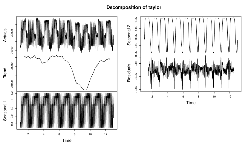
Figure 1: Decomposition of multiple seasonal time series according to msdecompose() function.

The classical decomposition does not typically produce clear components – the residuals in Figure 1 demonstrate the presence of seasonality because the approach assumes that the seasonal components are constant. Nonetheless, it can be a starting point for time series analysis. In smooth, it is used for the initialisation of states of ETS in case of seasonal data and is mainly needed when working with multiple seasonal data. However, if a researcher is interested in forecasting with seasonal decomposition, the function produces the object of the class smooth that supports the forecast() method, producing forecasts for the trend component of the decomposed data and then reconstructing the series based on the estimated seasonal components.

4 Exponential smoothing

Exponential smoothing is one of the most popular forecasting methods used in demand planning (Weller and Crone, 2012). As mentioned earlier, ETS underlies all exponential smoothing methods, and it is considered as an academic standard in forecasting (it has been used in all the major forecasting competitions over the years, including Makridakis and Hibon, 2000; Athanasopoulos et al., 2011; Makridakis et al., 2020, 2022). The conventional ETS model, developed by Hyndman et al. (2008) assumes that the error term follows normal distribution. It is implemented in functions ets() from the forecast package and ETS() from the fable. Their counterpart in smooth package is called es(), but it is based on the state space model (1) rather then the conventional one. Furthermore, while ets() supports only 15 ETS models, the es() implements all the theoretically possible 30 ETS models. The function also support fine tuning of parameters of model, allowing setting smoothing parameters values via persistence variable, initial values via initial and seasonal indices via initialSeason and pre-defining the values of parameters for the optimisation via the B parameter. Furthermore, the function supports explanatory variables via the xreg parameter, similar to how it is done in arima function from the stats package, allowing tuning the coefficients for regressors via initialX and selecting the most appropriate ones based on information criteria via the Sagaert and Svetunkov (2022) algorithm applied to residuals of the ETS model using the regressors parameter.

In terms of the ETS components selection, the mechanism used by default in es() can be summarised in the following steps:

1. Apply ETS(A,N,N) to the data, calculate an information criterion (IC);

2. Apply ETS(A,N,A) to the data, calculate IC. If it is lower than (1), then this means that there is some seasonal component in the data, move to step (3). Otherwise, go to (4);

3. Apply ETS(M,N,M) model and calculate IC. If it is lower than the previous one, then the data exhibits multiplicative seasonality. Go to (4);

4. Fit the model with the additive trend component and the seasonal component selected from the previous steps, which can be either “N”, “A”, or “M”. Calculate IC for the new model and compare it with the best IC so far. If it is lower than the criteria of previously applied models, then there is a trend component in the data. If it is not, then the trend component is not needed;

5. Form the pool of models based on steps (1) - (4), apply models and select the one with the lowest IC.

This approach for components selection can be called branch-and-bound because instead of going through all possible models, it considers branches of models. For example, if there is no seasonality, then the respective component can be set to “N”, thus removing the branch of seasonal models and reducing the pool of models to test from 30 to only 10 (including models already tested on the four steps).

Similarly to any other smooth function, es() supports several methods, including plot() for visual diagnostics of model and forecast() for forecasting. To demonstrate how they work, we apply es() to AirPassengers data from the datasets package.

    AirPassengersETS <- es(AirPassengers, h=12, holdout=TRUE)

In the code above, we have specified the forecast horizon of 12 steps ahead and asked to exclude the last 12 observations from the training of the model, thus creating a test set (holdout) to see how the model performs in that part of the data. We can do diagnostics of the model in order to see if it has any obvious issues that could be resolved:

    par(mfcol=c(2,2))
    plot(AirPassengersETS, c(1,2,4,6))

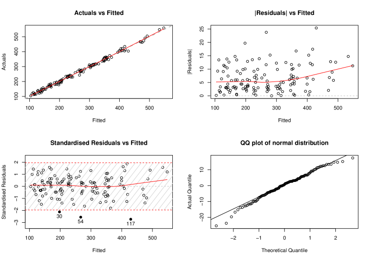
Figure 2: Diagnostics plots for ETS(A,M,M) model selected automatically on AirPassengers data by es() function.

The resulting plot is shown in Figure 2. We do not aim to resolve the issues of the model in this paper, we merely demonstrate what can be done using smooth functions. The plots allow analysing the residuals for the possible issues related to heteroscedasticity, autocorrelation, outliers, wrong specification etc. Fixing the issues can be done by including explanatory variables and/or changing the transformations used in the model. After fixing the potential issues a researcher can produce forecasts from the estimated model, which is done using the forecast() method from generics package (Wickham et al., 2022). But unlike the forecasting for the ets() and ETS(), the one from smooth supports several options, allowing choosing between a variety of prediction intervals (see documentation of forecast.smooth() method), allowing to produce one-sided interval (which is useful in case of pure multiplicative models on low-volume data, where the lower bound is typically equal to zero) and generating cumulative forecasts (which is useful in case of safety stock calculation in inventory management). We will use the default values of parameters, producing the parametric prediction interval:

    plot(forecast(AirPassengersETS, h=12))

The code above will result in the plot in Figure 3.

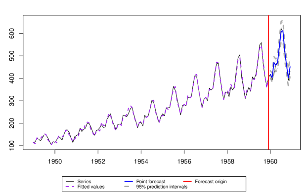
Figure 3: Forecast for AirPassengers data produced by es() function.

Figure 3 shows how the selected model fits the data, what point forecast it produces (solid bold blue line in the holdout part) and what prediction intervals it generated (a grey area in the holdout).

Continuing the theme of exponential smoothing, smooth also implements Complex Exponential Smoothing of Svetunkov et al. (2022) via the ces() function, which has the functionality similar to es() and supports the same set of methods.

Finally, as mentioned earlier, adam() implements ETS model as well and supports much more functionality. The main difference between the default ETS in adam() and es() is that the former supports distributions other than normal and, by default, uses Gamma distribution in case of multiplicative error models.

5 ARIMA

Another important model, which is used often in forecasting, is ARIMA (Box and Jenkins, 1976). There are several functions implementing ARIMA in SSOE state space form in the smooth package.

The ssarima() (State Space ARIMA) function implements a state space ARIMA in the form discussed in Chapter 11 of Hyndman et al. (2008). The function that implements the order selection for State Space ARIMA is called auto.ssarima(). It does not rely on any statistical tests and selects orders based on information criteria. Both the model and the selection mechanism are explained in Svetunkov and Boylan (2020).

The msarima() (Multiple Seasonal ARIMA) function relies on the state space model (1), introducing lagged components and thus substantially reducing the size of the transition matrix. This allows applying large multiple seasonal ARIMA models to the data. A thing to note is that because of this, the transition matrix, measurement, and state vectors of this model are formed differently than in Hyndman et al. (2008). In a general case, they are (Svetunkov, 2022, Chapter 9):

$$\begin{aligned} \mathbf{F}=\begin{pmatrix}\eta_{1}&\eta_{1}&\dots&\eta_{1}\\ \eta_{2}&\eta_{2}&\dots&\eta_{2}\\ \vdots&\vdots&\ddots&\vdots\\ \eta_{K}&\eta_{K}&\dots&\eta_{K}\end{pmatrix},&\mathbf{w}=\begin{pmatrix}1\\ 1\\ \vdots\\ 1\end{pmatrix},\\ \mathbf{g}=\begin{pmatrix}\eta_{1}+\theta_{1}\\ \eta_{2}+\theta_{2}\\ \vdots\\ \eta_{K}+\theta_{K}\end{pmatrix},&\mathbf{v}_{t}=\begin{pmatrix}v_{1,t}\\ v_{2,t}\\ \vdots\\ v_{K,t}\end{pmatrix},&\mathbf{l}=\begin{pmatrix}1\\ 2\\ \vdots\\ K\end{pmatrix}\end{aligned},$$ (5)

where $\eta_{j}$ is $j^{\text{th}}$ polynomial for the ARI part of the model, $\theta_{j}$ is the $j^{\text{th}}$ MA parameter and $K$ is the number of ARI/MA polynomials (whichever is the highest). To better understand how this model is formulated, consider an example of ARIMA(1,1,2), which can be written as:

$$(1-\phi_{1}B)(1-B)y_{t}=(1+\theta_{1}B+\theta_{2}B^{2})\epsilon_{t},$$ (6)

where $B$ is the backshift operator. This model can be written in the state space form (see Chapter 9 of Svetunkov, 2022, for derivations):

$$\begin{aligned} &y_{t}=v_{1,t-1}+v_{2,t-2}+\epsilon_{t}\\ &v_{1,t}=(1+\phi_{1})(v_{1,t-1}+v_{2,t-2})+(1+\phi_{1}+\theta_{1})\epsilon_{t}\\ &v_{2,t}=-\phi_{1}(v_{j,t-j}+v_{2,t-2})+(-\phi_{1}+\theta_{2})\epsilon_{t}\end{aligned}.$$ (7)

In order to see that the model (7) can be represented in the form (1), we need to set the following matrices and vectors:

$$\begin{aligned} \mathbf{F}=\begin{pmatrix}1+\phi_{1}&1+\phi_{1}\\ -\phi_{1}&-\phi_{1}\end{pmatrix},&\mathbf{w}=\begin{pmatrix}1\\ 1\end{pmatrix},\\ \mathbf{g}=\begin{pmatrix}1+\phi_{1}+\theta_{1}\\ -\phi_{1}+\theta_{2}\end{pmatrix},&\mathbf{v}_{t}=\begin{pmatrix}v_{1,t}\\ v_{2,t}\end{pmatrix},&\mathbf{l}=\begin{pmatrix}1\\ 2\end{pmatrix}\end{aligned}.$$ (8)

Finally, as mentioned earlier, adam() function supports ARIMA as well, in the same form as msarima(). All the three functions have similar syntax for ARIMA, where a user needs to defined seasonal lags of model via lags vector, listing all seasonal frequencies that a model should have, and orders of model via orders variable, which in general accepts a named list of the style orders=list(ar=c(1,2,3),i=c(1,2,3),ma=c(1,2,3)), defining the order of AR, I and MA parts of the model for the respective lags. The ARIMA orders are designed this way to allow researchers to introduce as many lags as they need, supporting, for example, double and triple seasonal ARIMA. Note that due to its formulation ssarima() cannot handle high-frequency data and will slow down with the increase of the seasonal lag $m$.

Here is an example of a user defined SARIMA(0,2,2)(0,2,2)₁₂ model applied to the same AirPassengers data:

    AirPassengersARIMA <- msarima(AirPassengers, lags=c(1,12),
                                  orders=list(i=c(2,2),ma=c(2,2)),
                                  h=12, holdout=TRUE)

In order to see how the model fits the data we can use the plot function, specifying which=7:

    plot(AirPassengersARIMA,7)

after which we will get the plot shown in Figure 4.

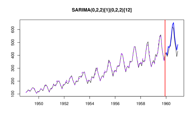
Figure 4: Forecast for AirPassengers data produced by msarima() function.

Furthermore, all the smooth functions support one of the three mechanisms of initialisation:

1. Optimisation – the initial values of the state vector are estimated during the optimisation stage;

2. Backcasting – the initial values are produced via applying the model with optimised parameters to the reversed data, going recursively from the last observation to the first one;

3. Manual – the initials are provided by a user.

These are regulated via the initial parameter in the functions. In the case of ARIMA, given the complexity of the task, initial="backcasting" typically works faster and more efficiently than the other two approaches.

If a researcher needs to have an ARIMA model with automatically selected orders, they can use auto.ssarima(), auto.msarima(), which will do that minimising the selected information criterion using the procedure described in Svetunkov and Boylan (2020) and in Section 15.2 of Svetunkov (2022). In case of adam(), the automatic selection mechanism is switched on via addition of variable select=TRUE in the list for the orders parameter.

ARIMA models produced using the three functions above supports all the methods available for other smooth functions, including plot(), actuals(), fitted(), residuals() and forecast().

6 Simulation functions

Another important set of functions supported by the smooth package is the simulation functions. They allow generating data from an assumed model. There are several functions in the package:

1. sim.es() allows generating data from the selected ETS model with defined persistence, initial and initialSeason parameters;

2. sim.ces() generates data from Complex Exponential Smoothing DGP;

3. sim.ssarima() generates data from ARIMA model, allowing defining order of the model, AR, MA parameters and the value of the constant term (either intercept or drift, depending on the order of differences).

If the parameters are not specified, they will be picked at random. All the functions above support a variety of distributions for the error term, allowing also to apply manually created ones. Here is an example of how to do the latter:

    customFunction <- function(n, mu, sd){
        return(log(abs(rnorm(n, mu, sd))));
    }
    x <- sim.es("ANN", obs=100,
                randomizer="customFunction", mu=0, sd=1)

The simulation functions allow generating as many series as needed, which is regulated via nsim parameter.

Finally, the package also implements simulate() method, which extracts the parameters from the already estimated model to generate simulated data from it. In order to see how it works, we generate data from the AirPassengersETS model, estimated in Section 4:

    x <- simulate(AirPassengersETS, obs=120, nsim=5)
    plot(x)

The code above will generate five time series, and each one of them would look similar to the one shown in Figure 5.

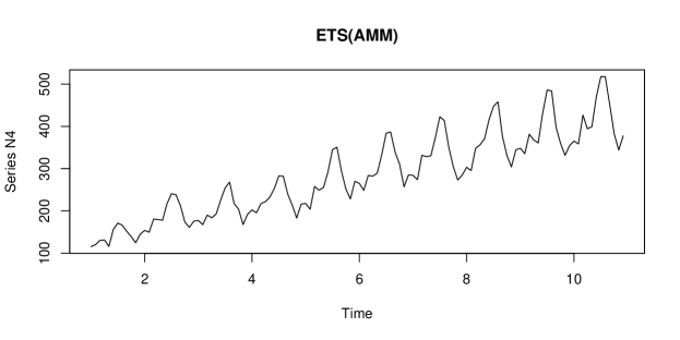
Figure 5: Simulated data from the AirPassengersETS model.

As can be seen from the plot in Figure 5, the generated time series exhibits behaviour similar to the original time series. It even has a similar seasonal shape, but it has a different trend, increasing slower than in the original data.

7 Other functions

There are several other functions implemented in the package that are outside of the scope of this paper. Nonetheless, two of them are worth mentioning.

There is a Simple Moving Averages (SMA) function, sma(), implemented in state space model (1). This is based on the paper of Svetunkov and Petropoulos (2018) who showed that SMA(p) has an underlying AR(p) process with parameters restricted to $\phi_{j}=\frac{1}{p}$ for all $j=1,\dots,p$. The function also supports automatic order selection via information criteria as discussed in the original paper.

Another important function is oes(), which implements the occurrence part of model in case of intermittent demand. This is discussed in detail in Chapter 13 of Svetunkov (2022) and is based on Svetunkov and Boylan (2019).

Last but not least, smooth package has extensive vignettes with examples of application of almost all functions. It is available, for instance, on CRAN: https://cran.r-project.org/package=smooth.

8 Benchmarking of smooth functions

Finally, to demonstrate how the smooth functions work, we conduct an experiment on M1 (Makridakis et al., 1982), M3 (Makridakis and Hibon, 2000) and Tourism (Athanasopoulos et al., 2011) competition data, where we evaluate seven models:

1. ADAM ETS – ETS model estimated via adam() function;

2. ADAM ARIMA – ARIMA model estimated via adam() function. We set model="NNN" to switch off ETS part of the model and use the following command to set the maximum ARIMA order to check:
   order=list(ar=c(3,2), i=c(2,1), ma=c(3,2), select=TRUE);

3. ES – ETS model implemented in es() function, which is just a wrapper of adam();

4. SSARIMA – State Space ARIMA model estimated via
   auto.ssarima();

5. CES – Complex Exponential Smoothing implemented in auto.ces() function from smooth package;

6. ETS – ETS model implemented in ets() function from forecast package;

7. ARIMA – ARIMA selected using auto.arima() function from
   forecast package.

We do not include msarima() in the experiment because the datasets under consideration do not have multiple seasonal time series. We have used the default values of parameters in all the functions. The forecasts were produced for each time series in the datasets for the horizons used in the original competitions to the part of the data not visible to the models. We produced point forecasts and 95% prediction intervals to that part of series and evaluated the performance of models using the following measures:

• MASE – Mean Absolute Scaled Error by Hyndman and Koehler (2006);

• RMSSE – Root Mean Scaled Squared Error introduced in Makridakis et al. (2022);

• Coverage – percentage of observations in the holdout lying in the produced 95% prediction interval;

• sMIS – scaled Mean Interval Score from Makridakis et al. (2022);

• Time – computational time in seconds spent for estimation and forecasts generation for each series.

For MASE, RMSSE, sMIS and time, the lower the value is, the better it is. For the coverage, the closer the value is to the nominal 95%, the better it is.

The results of this experiment are summarised in Table 1. Note that they might vary from one run to another because forecasts from some of the functions rely on simulations.

	MASE	RMSSE	Coverage	sMIS	Time
ADAM ETS	2.222	1.935	0.885	2.122	0.386
ES	2.224	1.939	0.898	2.196	0.477
CES	2.271	1.958	0.812	3.465	0.236
ETS	2.263	1.970	0.882	2.258	0.409
ARIMA	2.300	1.987	0.834	3.007	1.425
ADAM ARIMA	2.371	2.048	0.843	3.126	1.376
SSARIMA	2.480	2.133	0.802	3.356	1.811

Table 1: Error measures for each of the model evaluated on M1, M3 and Tourism competitions, aggregated using mean values. The boldface indicates the best performing models, while the italic indicates the second best ones.

As can be seen from Table 1, ADAM ETS outperforms all other models in terms of MASE, RMSSE and sMIS, although the difference between it and other ETS implementations does not look substantial. Note that it works slightly slower than CES. The ETS from forecast package performs slightly worse than the smooth implementations on these datasets. Comparing ARIMA implementations, the one from auto.arima() is more accurate and faster than ADAM ARIMA and SSARIMA, although it was not able to beat the ETS models. Note however that ARIMA produces lower coverage than ADAM ARIMA does and works slower.

This example demonstrates that the developed functions work efficiently and can be applied to a wide variety of time series. Table 1 summarises an overall aggregate performance, which does not mean that the winning models always perform the best. Their performance will vary from one series to another, and in some instances, the models that performed poorly in this experiment would perform much better (for example, SSARIMA performed very well on supply chain data with a short history as discussed in Svetunkov and Boylan, 2020).

9 Conclusions

In this paper, I have discussed the philosophy behind the models implemented in the smooth package for R. The state space model used in the functions differs from the conventional one, allowing to introduce more components and using more complex models efficiently. We have discussed how ETS and ARIMA are implemented in this framework and what an analyst can achieve with them. Finally, we have demonstrated how the models implemented in the smooth functions perform on an example of M1, M3 and Tourism competitions data.

This paper merely introduced the framework, the models and the functions. As mentioned earlier, the main idea of the smooth functions is to give a researcher flexibility. A reader interested in learning more about the framework is advised to read the online monograph of Svetunkov (2022) and to study examples in the vignettes of the smooth package in R (Svetunkov, 2023).

References

- Assimakopoulos and Nikolopoulos (2000) Assimakopoulos, V., Nikolopoulos, K., 2000. The theta model: a decomposition approach to forecasting. International Journal of Forecasting 16, 521–530.
- Athanasopoulos et al. (2011) Athanasopoulos, G., Hyndman, R. J., Song, H., Wu, D. C., 2011. The tourism forecasting competition. International Journal of Forecasting 27 (3), 822–844.
- Box and Jenkins (1976) Box, G., Jenkins, G., 1976. Time series analysis: forecasting and control. Holden-day, Oakland, California.
- De Livera et al. (2011) De Livera, A. M., Hyndman, R. J., Snyder, R. D., 2011. Forecasting Time Series With Complex Seasonal Patterns Using Exponential Smoothing. Journal of the American Statistical Association 106 (496), 1513–1527.
- Engle (1982) Engle, R. F., jul 1982. Autoregressive Conditional Heteroscedasticity with Estimates of the Variance of United Kingdom Inflation. Econometrica 50 (4), 987.
-
Gallego (2021)
Gallego, J. L., 2021. tfarima: Transfer Function and ARIMA Models. R package
version 0.2.1.
URL https://CRAN.R-project.org/package=tfarima - Hyndman and Khandakar (2008) Hyndman, R. J., Khandakar, Y., 2008. Automatic time series forecasting: the forecast package for R. Journal of Statistical Software 26 (3), 1–22.
- Hyndman and Koehler (2006) Hyndman, R. J., Koehler, A. B., 2006. Another look at measures of forecast accuracy. International Journal of Forecasting 22 (4), 679–688.
- Hyndman et al. (2008) Hyndman, R. J., Koehler, A. B., Ord, J. K., Snyder, R. D., 2008. Forecasting with Exponential Smoothing. Springer Berlin Heidelberg.
- Hyndman et al. (2002) Hyndman, R. J., Koehler, A. B., Snyder, R. D., Grose, S., 2002. A state space framework for automatic forecasting using exponential smoothing methods. International Journal of Forecasting 18 (3), 439–454.
-
Kaluzny and TIBCO Software Inc. (2021)
Kaluzny, S., TIBCO Software Inc., 2021. robustarima: Robust ARIMA Modeling. R
package version 0.2.6.
URL https://CRAN.R-project.org/package=robustarima - Koehler et al. (2012) Koehler, A. B., Snyder, R. D., Ord, J. K., Beaumont, A., 2012. A study of outliers in the exponential smoothing approach to forecasting. International Journal of Forecasting 28 (2), 477–484.
- Makridakis et al. (1982) Makridakis, S., Andersen, A. P., Carbone, R., Fildes, R., Hibon, M., Lewandowski, R., Newton, J., Parzen, E., Winkler, R. L., 1982. The accuracy of extrapolation (time series) methods: Results of a forecasting competition. Journal of Forecasting 1 (2), 111–153.
- Makridakis and Hibon (2000) Makridakis, S., Hibon, M., 2000. The M3-Competition: results, conclusions and implications. International Journal of Forecasting 16, 451–476.
- Makridakis et al. (2020) Makridakis, S., Spiliotis, E., Assimakopoulos, V., 2020. The M4 Competition: 100,000 time series and 61 forecasting methods. International Journal of Forecasting 36 (1), 54–74.
- Makridakis et al. (2022) Makridakis, S., Spiliotis, E., Assimakopoulos, V., oct 2022. M5 accuracy competition: Results, findings, and conclusions. International Journal of Forecasting 38 (4), 1346–1364.
-
O’Hara-Wild et al. (2021)
O’Hara-Wild, M., Hyndman, R., Wang, E., 2021. fable: Forecasting Models for
Tidy Time Series. R package version 0.3.1.
URL https://CRAN.R-project.org/package=fable -
R Core Team (2022)
R Core Team, 2022. R: A Language and Environment for Statistical Computing. R
Foundation for Statistical Computing, Vienna, Austria.
URL https://www.R-project.org/ - Sagaert and Svetunkov (2022) Sagaert, Y., Svetunkov, I., 2022. Trace Forward Stepwise: Automatic Selection of Variables in No Time.
- Snyder (1985) Snyder, R. D., 1985. Recursive Estimation of Dynamic Linear Models. Journal of the Royal Statistical Society, Series B (Methodological) 47 (2), 272–276.
-
Svetunkov (2022)
Svetunkov, I., 2022. Forecasting and analytics with adam. Monograph.
OpenForecast, (version: 2022-04-18).
URL https://openforecast.org/adam/ -
Svetunkov (2023)
Svetunkov, I., 2023. smooth: Forecasting Using State Space Models. R package
version 3.2.0.
URL https://github.com/config-i1/smooth - Svetunkov and Boylan (2019) Svetunkov, I., Boylan, J., 2019. Multiplicative state-space models for intermittent time series.
- Svetunkov and Boylan (2020) Svetunkov, I., Boylan, J. E., 2020. State-space ARIMA for supply-chain forecasting. International Journal of Production Research 58 (3), 818–827.
- Svetunkov et al. (2022) Svetunkov, I., Kourentzes, N., Ord, J. K., 8 2022. Complex exponential smoothing. Naval Research Logistics (NRL), 31.
- Svetunkov and Petropoulos (2018) Svetunkov, I., Petropoulos, F., 2018. Old dog, new tricks: a modelling view of simple moving averages. International Journal of Production Research 56 (18), 6034–6047.
- Taylor (2003) Taylor, J. W., 2003. Short-term electricity demand forecasting using double seasonal exponential smoothing. Journal of the Operational Research Society 54 (8), 799–805.
- Warren M. Persons (1919) Warren M. Persons, 1919. General Considerations and Assumptions. The Review of Economics and Statistics 1 (1), 5–107.
- Weller and Crone (2012) Weller, M., Crone, S. F., November 2012. Supply chain forecasting: Best practices & benchmarking study. Tech. rep., Lancaster Centre for Forecasting.
-
Wickham et al. (2022)
Wickham, H., Kuhn, M., Vaughan, D., 2022. generics: Common S3 Generics not
Provided by Base R Methods Related to Model Fitting. R package version 0.1.2.
URL https://CRAN.R-project.org/package=generics