Measuring out quasi-local integrals of motion from entanglement

I Abstract

Quasi-local integrals of motion are a key concept underpinning the modern understanding of many-body localisation, an intriguing phenomenon in which interactions and disorder come together. Despite the existence of several numerical ways to compute them - and astoundingly in the light of the observation that much of the phenomenology of many properties can be derived from them - it is not obvious how to directly measure aspects of them in real quantum simulations; in fact, the smoking gun of their experimental observation is arguably still missing. In this work, we propose a way to extract the real-space properties of such quasi-local integrals of motion based on a spatially-resolved entanglement probe able to distinguish Anderson from many-body localisation from non-equilibrium dynamics. We complement these findings with a new rigorous entanglement bound and compute the relevant quantities using tensor networks. We demonstrate that the entanglement gives rise to a well-defined length scale that can be measured in experiments.

II Introduction

It is widely believed that generic quantum systems isolated from their environments will evolve under their own dynamics until they reach an apparent equilibrium state that locally resembles the expectations of a thermal equilibrium state Polkovnikov et al. (2011); Gogolin and Eisert (2016). This expectation is seen as a stepping stone to reconcile predictions from statistical mechanics and those of basic quantum mechanics. One major exception to this rule is the case of low-dimensional quantum systems in the presence of random disorder. Non-interacting quantum systems in one dimension will entirely fail to thermalise due to any finite concentration of disorder Anderson (1958), and in recent decades it has been shown that interacting many-body systems appear to suffer the same fate Fleishman and Anderson (1980); Basko et al. (2006), leading to the phenomenon now known as many-body localisation (MBL) Huse et al. (2013, 2014); Altman and Vosk (2015); Luitz et al. (2015); Alet and Laflorencie (2018); Abanin et al. (2019); Friesdorf et al. (2015). From a theoretical standpoint, MBL is now fairly well understood in terms of the emergence of an extensive number of conserved quantities known as (quasi-)local integrals of motion (LIOMs, also known as localised bits or $l$-bits) which can prevent many-body systems from reaching thermal equilibrium Huse et al. (2014); Serbyn et al. (2013). While phenomenological models based around the concept of $l$-bits have seen great success Ros et al. (2015); Imbrie et al. (2017), and there are several approaches that can map microscopic models onto effective $l$-bit models Rademaker and Ortuño (2016); Rademaker et al. (2017); Pekker et al. (2017); Goihl et al. (2018a); Thomson and Schiró (2018); Kulshreshtha et al. (2019); Thomson and Schiró (2020); Thomson et al. (2021); Thomson and Schirò (2023); Thomson (2023); Bertoni et al. (2022), the $l$-bits themselves remain a strictly theoretical construct, inaccessible to any experimental probes. This is in contrast with the case of Anderson localised systems, where the exponentially localised $l$-bits can be straightforwardly related to the real-space decay of the single-particle states, which has been experimentally observed Billy et al. (2008).

Figure 1: Division into subsystems and computation of negativity: a) A sketch showing how a one-dimensional spin chain is partitioned into three subsystems. We are interested in computing the entanglement between subsystems $A$ and $B$ after subsystem $C$ has been traced out, giving rise to a spatially-resolved entanglement measure. b) Sketch of the initial quantum state in matrix product operator (MPO) form, made by taking the outer product of two matrix product state vectors. c) Sketch of how the negativity is computed: the partial transpose of subsystem $A$ corresponds to ‘twisting’ the MPO legs while tracing out subsystem $C$ corresponds to contracting the relevant MPO indices.

In this work, we propose an experimentally feasible approach to measuring the actual real-space properties of local integrals of motion in many-body quantum systems using the entanglement negativity, a sensitive entanglement monotone that allows for the recovery of spatially resolved entanglement information. In this way, we accommodate the above missing link. Various quantities capturing correlations and entanglement, including the negativity, have been measured in recent experiments with ultra-cold bosons: Ref. Lukin et al. (2019) has measured single-site and half chain number and configurational entanglement for a system subject to a quasi-periodic potential. These can be seen as a witness detecting the absence of thermalization, but they do not provide a length scale. The authors have also measured classical density-density correlations—akin to the proposal of Ref. Goihl et al. (2019)—showing exponentially decaying correlations, but this is a two-point classical measure, in contrast to the genuine entanglement between two half-regions considered here. Reference Chiaro et al. (2022) has studied a disordered system and has shown that the entanglement negativity can be directly measured. In a first experiment, the authors of the latter work prepared the system in a product state and measured the two-qubit entanglement of formation as they vary the separation between the qubits. While this setting is close in spirit to our approach, they have chosen a two-qubit setting, which is the only setting in which one can compute this quantity, so that the diagnostic time scale that allows observation of any spatial dependence is short. In a second experiment, the preservation of entanglement has been studied, departing from the approach taken here. Here, we demonstrate that the negativity itself gives direct access to a unique length scale that characterises the $l$-bits.

III Results and Discussion

Quasi-local operators. The question of whether many-body localisation is a well-defined stable phase in the thermodynamic limit remains unsettled, nevertheless systems showing MBL-like phenomenology for experimentally accessible times and system sizes appear to be well described by $l$-bit models, and their length scale is physically meaningful regardless of whether this description keeps holding for very long times and very large system sizes. Since the goal of the present work is to characterize the $l$-bits, we will now give precise definitions of what they are and the role they play in the dynamics.

Definition 1 (Quasi-local operators).

An operator $O$ on the lattice $\Lambda$ is said to be quasi-local around a region $R$ with localisation length $\xi$ if for any region $X\subset\Lambda$ containing $R$

$$\left|\left|O-\frac{1}{2^{|X^{c}|}}{\rm tr}_{X^{c}}(O)\otimes\mathbb{I}_{X^{C}c}\right|\right|^{2}\leq\|O\|^{2}\,Ke^{-d(R,X^{c})/\xi}$$ (1)

where $K>0$ is a universal constant, $X^{C}$ denotes the complement of $X$, $d(X^{c},R)=\mathchoice{\operatorname*{min}}{\operatorname*{min}}{\mathrm{min}}{\mathrm{min}}_{x\in X^{c},r\in R}d(x,r)$ is the length of the shortest path from $X$ to $R$, and $\|\cdot\|$ is the normalized 2-norm, $\|O\|^{2}={{\rm tr}{OO^{\dagger}}}/{{\rm tr}{I}}$.

Intuitively, this definition says that most of the support of $O$ is concentrated in and immediately around the region $R$, in the sense that if we truncate $O$ to an operator only supported on a sphere centered at $R$, the resulting operator differs from $O$ only by an error decaying exponentially in the radius of the sphere. Interestingly, the relatively loose sense of decay in $2$-norm seems crucial, an insight that is often under-appreciated Goihl et al. (2018b); Ilievski et al. (2016). It is important to note that this is an abstract definition: it does not give operational advice on how to find those $l$-bits. What is more, even if they exist, they are by no means unique Chandran et al. (2015). There could be “more local” $l$-bits than those given that still give rise to a complete set of $l$-bits. Either way, as is common, such $l$-bits serve as our definition for many-body localisation.

Definition 2 (Many-body localisation).

A Hamiltonian

$$H=\sum_{j=1}^{n}\omega_{j}^{(1)}h_{j}+\sum_{j,k=1}^{n}\omega^{(2)}_{j,k}h_{j}h_{k}+\dots$$ (2)

with real weights $\{\omega_{j}^{(1)}\}$ and $\{\omega_{j,k}^{(2)}\}$, is called many-body localised if it can be written as a sum of mutually commuting ($[h_{j},h_{k}]=0$ for all $j,k$) quasi-local terms $h_{j}$, each centred around site $j$, and if $\omega_{i_{1},\dots,i_{n}}\leq\omega e^{-|i_{1}-i_{n}|/\kappa}$ for some constant $\kappa>0$, where $i_{1}<i_{2}\dots<i_{n}$.

In other words, a many-body localized Hamiltonian can be written as an effective model which is classical, in the sense that all Hamiltonian terms commute, and quasi-local, in the sense that the total coupling strength between two sites decays exponentially with distance.

Premise of the approach. When written in the basis that diagonalises the Hamiltonian, as in Eq. (2), these $l$-bits are strictly local objects, but in real-space they are quasi-local with exponentially decaying tails. In order to extract properties of $l$-bits from experiments, we shall consider the evolution of an arbitrary initial state under the following Hamiltonian dynamics as

$$\rho(t)=e^{-itH}\rho e^{itH},$$ (3)

for times $t\geq 0$. To simplify the notation, we will suppress the time argument for time $t=0$. How can this time evolution be exploited to measure out real-space properties of the $l$-bits? Some intuition can be attained in the situation when the $\{h_{j}\}$ are strictly local. The terms that do not overlap do not contribute to the entanglement evolution at all. So in the end, it is the overlapping tails that will lead to entanglement growth.

Model. We will demonstrate our scheme numerically using the ‘standard model’ of MBL, namely the XXZ spin-1/2 chain with random on-site fields, while it should be clear that the approach taken would be applicable to any many-body localised model. Its Hamiltonian is given by

$$H=J_{0}\sum_{i}\left(S^{x}_{i}S^{x}_{i+1}+S^{y}_{i}S^{y}_{i+1}+\Delta S^{z}_{i}S^{z}_{i+1}\right)+\sum_{i}h_{i}S^{z}_{i},$$ (4)

with $h_{i}\in[-d,d]$. We shall set $J_{0}=1$ as the unit of energy throughout, with $\Delta=1.0$ unless otherwise stated, and will use open boundary conditions. This model has been thoroughly studied and shown to exhibit a phase with anomalous thermalisation properties above a disorder strength of $d\gtrsim 3.7$ Luitz et al. (2015), although recent work has suggested that the true phase transition in the thermodynamic limit could be at much larger values of $d$ if it exists at all Doggen et al. (2018); Šuntajs et al. (2020a, b); Sels and Polkovnikov (2023, 2021).

The characteristic growth in time of the von Neumann entanglement entropy  Bardarson et al. (2012); Znidaric et al. (2008) (or its correlation-based analogues Goihl et al. (2019)) mentioned above has been shown to be a good indicator of many-body localisation, able to distinguish it from single-particle Anderson localisation via the late-time logarithmic growth. Motivated by this, our aim in this work is to show that other entanglement measures which provide spatially-resolved information can not only distinguish many-body localisation from Anderson localisation, but can also allow direct quantitative measurement of the properties of many-body local integrals of motion.

Diagnostic entanglement quantity. The main quantity of interest in this work is the logarithmic negativity, a measure of the entanglement between two subsystems of the spin chain, denoted $A$ and $B$, separated by a distance $r$, which together with $C$ constitutes the entire system (sketched in Fig. 1). It is defined as Życzkowski et al. (1998); Eisert and Plenio (1999); Vidal and Werner (2002); Plenio (2005)

$$E_{N}(\rho_{A,B}(t)) :=\log_{2}(\|\rho_{A,B}^{T_{A}}(t)\|_{1}),$$ (5)

where $\|O\|_{1}={\rm tr}|O|$ denotes the trace norm, $\rho_{A,B}(t)={\rm tr}_{\backslash\{A,B\}}[\rho(t)]$ is the time-dependent quantum state of subsystems $A$ and $B$ after tracing out all other lattice sites, and the superscript $T_{A}$ indicates the partial transpose with respect to subsystem $A$. This has been shown to be an entanglement monotone meaningfully quantifying entanglement Eisert (2001); Vidal and Werner (2002); Plenio (2005). In the following, we shall refer to this quantity simply as ‘negativity’. By contrast to the more commonly studied bi-partite von Neumann or Rènyi entanglement entropies which consider a single bi-partition between two connected subsystems, the entanglement negativity allows for a meaningful spatially resolved measure of mixed-state entanglement, as the two subsystems can be separated by an arbitrary distance $r:={\rm dist}(A,B)$, a feature the von Neumann entropy cannot capture as a pure state entanglement measure. This measure can also be used to study the entanglement between subsystems of arbitrary size. However, for conceptual clarity, we shall mainly consider $A$ and $B$ to cover the entire chain except for a piece $C$ with $|C|=r+1$ separating $A$ and $B$, as shown in Fig. 1. That said, the concept works as well for small regions $A$ and $B$, as they are accessible in experiments and are discussed in the rigorous bounds. Numerical evidence is shown in Supplementary Note 5. The negativity has previously been investigated in the context of ground states of disordered spin chains Ruggiero et al. (2016), quenches in random spin chains Ruggiero and Turkeshi (2022), the many-body localisation transition Gray et al. (2019), and quench dynamics in the presence of a defect Gruber and Eisler (2020). For clarity, in the following, we shall drop the explicit dependence of $E_{N}$ on the quantum state and instead use the notation $E_{N}(r,t)$ to represent the negativity associated to two subsystems separated by a distance $r$ and a time $t$ following a quench from an initial product state, emphasizing that this is indeed a spatially resolving entanglement measure.

A heuristic argument for why this quantity is relevant in our case can be given in the following manner. Ref. Serbyn et al. (2013) has shown that the von Neumann entanglement entropy grows in time following a quench according to $S_{\rm ent}\propto\ln(J_{0}t/\hbar)$, once the system enters the late-time equilibration regime. If we wish to consider the entanglement negativity between two subsystems separated by a distance $r$, a reasonable starting assumption is that the negativity will vary in time according to the same $\sim\ln(t)$ growth but will be exponentially suppressed in magnitude due to the spatial separation of the two subsystems, leading to an overall behaviour of $E_{N}\propto\exp(-r/\xi)\ln(J_{0}t/\hbar)$. We shall show that this ansatz is a good match for the numerical results. We also wish to emphasise that this logarithmic growth is characteristic of the interacting system and is entirely absent from Anderson-localised systems, meaning that the existence of this length scale is a distinct fingerprint of a many-body localised system.

Corroborating the reasoning with rigorous bounds. We see that Hamiltonians that are many-body localised in the sense of Definition 2 create entanglement at a rate that decays exponentially in the distance $r={\rm dist}(A,B)$ between parts $A$ and $B$, reflecting the exponential decay of the tails in quasi-local $l$-bits. In fact, not only this intuition can be made entirely rigorous, but, at the cost of slightly weakening the definition of quasi-locality, we are in the position to state precise upper bounds for the negativity for all times and distances.

Theorem 1 (Rigorous entanglement bounds).

Let $\rho$ be an initial product state. Let $H$ be a many-body localised Hamiltonian as per Definition 2 with localisation length $\xi<{1}/({4\log(2)})$ and $2(1/\kappa-\log(2))>1/\xi$, consider three blocks $A,C,B$ such that $C$ divides $A$ from $B$, with $|C|=r+1$. The growth of the negativity of the state $\rho(t)=e^{-itH}\rho e^{itH}$ restricted to the regions $A,B$ is bounded as

$$E_{N}(r,t)\leq\mathchoice{\operatorname*{min}}{\operatorname*{min}}{\mathrm{min}}{\mathrm{min}}\{t\,O(e^{-r/(2\xi)}),8\xi\log_{2}(t)-2r\}+O(1),$$ (6)

for times $t\geq e^{r/(4\xi)}$, while for $t<e^{r/(4\xi)}$,

$$E_{N}(r,t)\leq t\,O(e^{-r/(4\xi)}).$$ (7)

We hence find a short time behaviour signifying a linear growth in time, a cross-over regime governed by the correlation length, and a logarithmic growth for long times. These bounds—interesting in their own right and complementing and refining those of Ref. Kim et al. (2014)—are perfectly compatible with the above numerical assessment. In Supplementary Note 8, we state details of the proof of the bound that makes extensive use of the precise form of the tails of the $l$-bits. Based on our numerical results, we expect that our assumptions on the localisation length and the definition of quasi-locality can be relaxed without affecting the result. We also note that the observed $\xi-$dependence of the late time decay of the entanglement with the size of $C$ is not visible in this bound, though we expect that it can be refined to show this.

Figure 2: Behaviour of entanglement negativity in time and space: Results showing the growth of the negativity $E_{N}(r,t)$ with time for different distances $r$. Data is shown for a system size $L=24$ and a disorder strength $d=8.0$, averaged over $N_{s}=100$ disorder realisations. a) The dynamics of $E_{N}(r,t)$ following a quench from a Nèel state, showing the logarithmic growth at late times. The circular markers are the raw data points, while the solid lines are a smoothed guide to the eye. The error bars indicate the standard error in the mean. We note that these error bars show agreement on average between the various disorder realizations, but they are not fully statistically independent errors, as would be expected in an experiment where each data point would come from a different run. b) The full dynamics of $E_{N}(r,t)$, reflecting the logarithmic ‘light cone’. Each circle maps the point where the negativity grows beyond the corresponding threshold $\varepsilon$ and the lines are linear fits. c) By extracting the behaviour of $E_{N}(r,t^{*})\propto\exp(-r/\xi)$ at fixed times $t^{*}$ [dashed vertical lines in panel (a), horizontal lines in panel (b)], we can extract a well-defined length scale $\xi(t)$, which depends only weakly on time. The solid lines indicate the fits to the data points which are used to extract the $l$-bit length scale, demonstrating convergence at late times.

Numerical results. We first discuss qualitatively the results for the growth of the entanglement negativity with time for various different distances $r$, as shown in Fig. 2a) for a disorder strength $d=8.0$ (deep in the localised phase), where we find that indeed the negativity grows logarithmically with time at late times. Results for further disorder strengths, system sizes, and subsystem sizes are available in Supplementary Notes 2,3,4 and 5. At short times, the negativity is dominated by diffusive transport on length scales shorter than the localisation length. At large distances $r$, the negativity remains close to zero until a time exponentially large in $r$, which can be used to define a ‘light cone’ that characterises the spreading of the entanglement negativity, shown in Fig. 2b). The three lines indicate when the negativity grows above a threshold $\varepsilon\in\{0.0001,0.001,0.005\}$, mapping out an approximately logarithmic light cone. As the negativity outside of this length cone is exponentially small, in the following analysis, we restrict ourselves to space-time coordinates $(r,t)$, which are within the light cone. The existence of this light cone means that we gain only diminishing returns by going to larger system sizes: although we are able to separate the subsystems by a larger value of $r$, the evolution time required to obtain meaningful entanglement scales exponentially in $r$, which incurs a large computational cost for large systems and quickly becomes prohibitive.

In the late-time logarithmic growth regime, where the dynamics are dominated by the quasi-local nature of the $l$-bits, we extract the value of the negativity at a given time $t^{*}$ following the quench from an initial Néel state and plot it versus the subsystem separation $r$. We show this in Fig. 2c) for several different choices of time $t^{*}$ [indicated by the dashed lines in Fig. 2a)]. The data points form a straight line (on a logarithmic scale), and at late times the gradient of the line does not strongly change with the choice of time $t^{*}$, appearing to saturate at a fixed value (although the y-axis offset will, of course, continue to increase in time). Further details are available in Ref. Under the assumption that the negativity decays exponentially with distance like $E_{N}(r,t^{*})\propto\exp(-r/\xi)$, we can perform a linear fit to the data shown in Fig. 2c) and extract a well-defined length scale $\xi$ which characterises the spatial extent of the $l$-bits. The results are shown in Fig. 3, where we find that the length scale $\xi$ exhibits monotonic decay with increasing disorder strength, as expected. Note that no assumptions are involved other than the exponential decay of the negativity with distance at some fixed time $t^{*}$: the resulting length scale is an emergent property of the many-body system. This assumption does not hold in the delocalised phase, where the entanglement does not enter a regime of logarithmic growth. We can further compare the length scale extracted from our procedure with the $l$-bit decay lengths computed using the established numerically exact method of Ref. Goihl et al. (2018b), using the definition of quasi-locality from Eq. (1). We find excellent agreement between the entanglement-based length scale and the $l$-bit localisation length obtained independently from this method, confirming that the length scale probed by the negativity is the localisation length of the $l$-bits.

Figure 3: Extracted l-bit length scale: The characteristic $l$-bit length scale $\xi$ extracted from the entanglement negativity at time $t^{*}=500$, shown in blue for $L=24$ with $N_{s}\in[50,100]$ disorder realisations and various values of the disorder strength $d$. Error bars indicate the fit error and are roughly the same size as the plot markers. Orange lines mark the localisation length obtained through exact diagonalisation following Ref. Goihl et al. (2018b). For further details on calculating the localisation length using exact diagonalisation, see Supplementary Note 7 SM . The black line indicates the localisation length of the corresponding Anderson-localised system, obtained by directly diagonalising the Hamiltonian in the non-interacting limit ($\Delta=0$), for a system of size $L=128$ with $N_{s}=10000$.

For comparison, we also indicate the corresponding localisation length of an Anderson localised system, here obtained by directly diagonalising the Hamiltonian with $\Delta=0$ (following a Jordan-Wigner transform into the fermionic representation). We compute the eigenvectors of the Hamiltonian in the non-interacting setting, which decay in real space as $\exp(-r/\xi)$ Lee and Ramakrishnan (1985), average over disorder realisations and extract the localisation length $\xi$ from a least-squares fit. The length scale extracted from the TEBD data behaves in a qualitatively similar manner to the single-particle localisation length but is always larger, confirming that we are not measuring single-particle properties but are indeed extracting a genuinely many-body feature of the system. In the delocalised phase, our assumed form of the negativity is no longer valid, and as such, the method cannot extract a reliable length scale.

We also note that the entanglement negativity is not the only entanglement measure which may be used in this way: any spatially-resolved entanglement probe should behave similarly. In Supplementary Note 6, we demonstrate that the mutual information also gives consistent results.

IV Conclusion

In this work, we have outlined an experimentally feasible procedure for measuring local integrals of motion based on their contribution to the slow growth of the negativity at long times following a quench from an arbitrary initial state. We have demonstrated that the length scale which we obtain from this procedure, which characterises the $l$-bits, is in good agreement with that obtained using other theoretical methods in the literature. The crucial advantage is that our scheme is experimentally tractable, unlike other purely theoretical/numerical methods, which cannot be verified in real experiments. It would be extremely interesting to apply this method to other scenarios where many-body localisation is believed to exist, such as in disorder-free systems and two-dimensional models, in order to see if well-defined length scales based on the spreading of entanglement may still be extracted in these situations. This work paves the way for the application of spatially-resolved entanglement probes to phenomena in quantum simulation beyond many-body localisation, where such methods may be able to provide valuable insight into emergent length scales associated with other types of quasi-particles.

V Methods

We compute the negativity using time-dependent matrix product state simulations – an instance of a tensor network method Orús (2014) – implemented in the Quimb package Gray (2018a) using the time-evolving block decimation (TEBD) algorithm to perform the evolution Vidal (2004); Schollwöck (2011), with the system initially prepared in a Néel state. We use system size $L=24$ with a maximum bond dimension of $\chi=192$. We perform the time evolution using a maximum time step $dt=0.05$, at each step discarding singular values smaller than $\epsilon=10^{-10}$. We have checked that the results are well-converged. Detailed benchmarks are shown in Supplementary Note 1. Our TEBD results are compared against $l$-bit length scales obtained using exact diagonalisation, following Ref. Goihl et al. (2018b).

The negativity can be computed straightforwardly from a matrix product state (MPS) representation Gray (2018b). The state vector can be turned into a matrix product operator (MPO) (sketched in Fig. 1) representing the quantum state by considering vectors and dual vectors represented as MPS. The partial transpose can be computed by ‘twisting’ the legs of the MPO tensors, while the partial trace over the subsystem $C$ can be performed by contracting the free indices of the MPO tensors in this subsystem. At long times, the negativity should saturate at a value controlled by the size of the subsystems, and at any time $t<t^{s}$ (where $t^{s}$ is the saturation time), the negativity should satisfy the hierarchy $E_{N}(r_{1},t)<E_{N}(r_{2},t)$ for any two distances $r_{1}>r_{2}$.

VI Data availability

The full data for this work is available at Ref. Lu et al. (2022).

VII Code availability

The full code for this work is available at Ref. Thomson (2022).

VIII Author contributions

JE initially conceived the project. BL and JE jointly developed the idea of using entanglement bounds. SJT and BL wrote the code and performed the simulations. CB and JE proved the entanglement growth bound. All authors contributed to the writing of the final manuscript.

IX Acknowledgements

This project has been inspired by discussions with P. Roushan and B. Chiaro of Google AI. We also thank A. Kshetrimayum, S. Sotiriadis, S. Qasim, and J. Gray for discussions. B. Lu is grateful for feedback from D. Abanin, M. Fleischhauer, and M. Kiefer-Emmanouilidis at the CRC 183 summer school “Many-body physics with Rydberg atoms”. We gatefully acknowledge D. Toniolo for finding an error in an earlier draft of this work. This project has received funding from the European Union’s Horizon 2020 research and innovation programme under the Marie Skłodowska-Curie grant agreement No. 101031489 (Ergodicity Breaking in Quantum Matter), the Quantum Flagship (PASQuanS2),the Munich Quantum Valley, the Deutsche Forschungsgemeinschaft (CRC 183 and FOR 2724), and the ERC (DebuQC). We also acknowledge funding from the BMBF (FermiQP and MUNIQC-ATOMS).

Appendix A Supplementary information

Appendix B Supplementary note 1: TEBD accuracy benchmarks

As TEBD does not precisely conserve the energy of the initial state, as a benchmark of the accuracy of our numerics we compute the relative error in the energy of the time-evolved state vector, $E(t)=\braket{\psi(t)}{H}{\psi(t)}$, computed with respect to its energy at time $t=0$. The relative error is defined as

$$\delta E(t):=\left|\frac{E(t)-E(t=0)}{E(t=0)}\right|.$$ (8)

Fig. S1 shows the relative error versus time for a variety of different disorder strengths. We find that in most cases, the relative error remains close to $\delta E\approx 0.001$, i.e., the energy is conserved up to an error of approximately one-tenth of a percent, confirming that our simulations are reliable.

Fig. S1: Relative error of the simulation: A comparison of the relative error in the energy of the time-evolved state for different values of the disorder strength $d$, shown for system sizes $L=14$ ($\chi=128$, averaged over $N_{s}=240$ disorder realisations) and - at strong disorder only - $L=24$ ($\chi=192$, averaged over $N_{s}=100$ disorder realisations). The relative error remains below $1\%$ for all disorder strengths. Error bars indicate the variance over disorder distributions and in most cases, are of comparable size to the plot markers.

Appendix C Supplementary note 2: Comparison of disorder strengths

In addition to the data presented in the main text, here we show the behaviour of the entanglement negativity over a range of different disorder strengths, demonstrating the logarithmic growth at late times in the localised phase, and the qualitatively different behaviour seen in the delocalised phase. The results are shown in Fig. S2, for a system of size $L=14$, bond dimension $\chi=128$, and averaged over $N_{s}=240$ disorder realisations. The circle markers represent the data points, while the solid lines are smoothed guides to the eye. Deep in the delocalised phase ($d=1.0$), we see that the negativity saturates for all values of $r$ at relatively early times, making it difficult to pinpoint a regime where the growth of the negativity can be associated with a length scale. In contrast, the negativity in the localised phase increases much more slowly with time, and the spacing of the curves is consistent with an exponential suppression of the negativity with distance, as demonstrated in the main text.

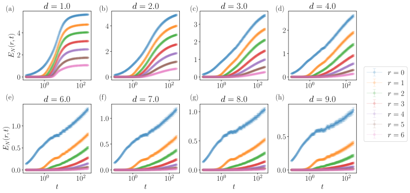
Fig. S2: Entanglement negativity at different disorder strengths: A comparison of the dynamics of the entanglement negativity $E_{N}(r,t)$ for different values of the disorder strength $d$, shown for $L=14$ with bond dimension $\chi=128$ and averaged over $N_{s}=240$ disorder realisations. In the delocalised phase, the negativity saturates to a value determined by the size of the subsystems $A$ and $B$, while in the localised phase the negativity displays a slow $\propto\log(t)$ growth even at late times. In this dephasing regime, we are able to use the data shown here to extract a length scale that characterises the localised phase, as detailed in the main text.

Appendix D Supplementary note 3: Bond dimension

In Fig. S3, we show the negativity dynamics for system size $L=24$ and varying bond dimension $\chi$, demonstrating that for $\chi=192$ (the choice used in the main text) the results are well-converged. The crucial factor for our work is the rate of growth of the negativity, which appears largely unaffected by the choice of bond dimension, although deviations can be seen for the smallest value shown in Fig. S3.

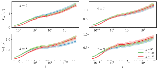
Fig. S3: Entanglement negativity for different bond dimensions and disorder strengths: The dynamics of the negativity $E_{N}(r,t)$ with $r=0$, for different bond dimensions and disorder strengths. Data shown is for $L=24$, averaged over $N_{s}=100$ disorder realisations. Error bars show the standard error.

Appendix E Supplementary note 4:Comparison of different measurement times

In the main text, all results for the length scale $\xi\equiv\xi(t^{*})$ are taken with $t^{*}=500$, i.e., the maximum evolution time of our simulations, however, it is clear from the negativity dynamics that there should be a weak dependence of $\xi$ on the measurement time $t^{*}$. Here we demonstrate this effect. Figs. S4 and S5 show how the linear fit used to extract the decay of $E_{N}(r,t)$ against $r$ depends on the choice of time $t^{*}$ for a variety of different disorder strengths, and Fig. S6 shows how the resulting values of $\xi(t^{*})$ change as $t^{*}$ and $d$ are varied. At short times there is a visible change in the length scale $\xi(t)$, however, at longer times we see that it appears to saturate towards a well-defined length scale with only a weak dependence on time. It is possible that simulations which extend to longer times may be able to improve upon the results presented here, but our results suggest this will be a meagre quantitative improvement in exchange for a great deal of computational effort.

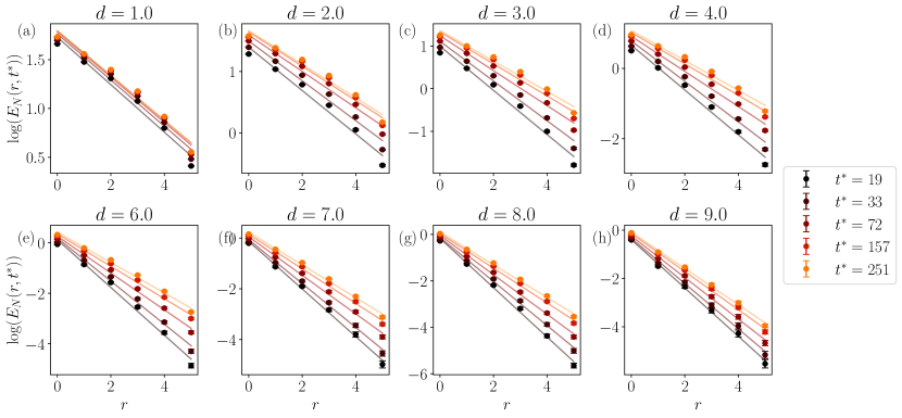
Fig. S4: Fits of the spatial decay of entanglement negativity for different times and disorder strengths: A comparison of the fits to the entanglement negativity $E_{N}(r,t^{*})$ at different times $t^{*}$ and for different values of the disorder strength $d$, shown for $L=14$ and averaged over $N_{s}=240$ disorder realisations. The circular markers show the data, while the solid lines indicate the linear fits used to extract the $l$-bit localisation length. Error bars showing the standard error in the mean are typically smaller than the marker size. At large disorder strengths (i.e., in the localised phase), the linear fit is very good, confirming that the negativity does indeed decrease exponentially with distance in this phase. After a time of $t^{*}\approx 100$, the gradient of the decay (and hence the corresponding $l$-bit localisation length) does not strongly change with time in the localised phase.

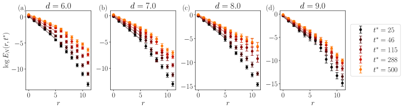
Fig. S5: Fits of the spatial decay of entanglement negativity for different times and disorder strengths: The same as in Fig. S4, but for $L=24$, $\chi=192$ and averaged over $N_{s}=100$ disorder realisations, shown only in the localised phase. The solid lines indicate the range of points over which the exponential fits were performed in order to extract the length scale shown in Fig. 3 of the main text.

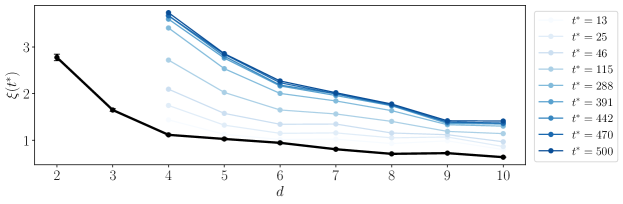
Fig. S6: Extracted length scales at different times: A comparison of how the length scale $\xi(t^{*})$ changes as the measurement time $t^{*}$ is varied. The results here are extracted from the fits shown in Fig. S5. At short times, the value of $\xi(t^{*})$ changes rapidly, however, at longer times, the dependence of $t^{*}$ weakens significantly. The black line is the Anderson localisation length for comparison, as discussed in the main text. For clarity, error bars are not shown except on the Anderson localisation length. (Note that error bars are shown in the data presented in the main text.)

Appendix F Supplementary note 5: Negativity between subsystems of fixed size

It is also possible to compute the entanglement negativity on a more general interval between two subsystems of fixed size $R_{b}$ separated by a distance $r$, as sketched in Fig. S7. In this case, a very similar procedure to that proposed in the main text is possible, with the caveat that one must carefully choose both the block size $R_{b}$ and the distance $r$ to ensure that the extraction of the $l$-bit length scale is done during the dephasing regime.

To be specific, if the block size $R_{b}$ is small and the subsystems are close together (i.e., $r$ is small), then the entanglement negativity will rapidly saturate (as the maximum entanglement is controlled by the size of the subsystems under consideration). On the other hand, if the blocks are widely separated (i.e., large $r$), then the negativity will remain zero until times exponentially large in $r$. If one were to consider a small subsystem of $R_{b}=2$, for example, then the entanglement negativity for small values of $r$ would saturate well before widely separated subsystems have time to become entangled, this meaning that the data points for both small $r$ and large $r$ would have to be discarded when performing the fit. This can be ameliorated by using blocks of intermediate size, such that they are large enough that the subsystem entanglement does not saturate too rapidly and the data at small values of $r$ remains reliable. Representative results for this case are shown in Fig. S8, where it is clear that for block size $R_{b}=2$, the curves for small values of $r$ saturate too quickly to be used in extracting the $l$-bit length scale. Block size $R_{b}=3$ is better, and here $R_{b}=4$ offers the best compromise, with a clearly identifiable region where the curves for all values of $1\leq r<5$ are in a regime of logarithmic growth with approximately the same rate, and a length scale may be extracted. On the other hand, for block size $R_{b}=5$, with a system size of $L=16$ it is not possible to separate the blocks widely enough to extract enough data to perform a reliable fit. (Note that in these computations, we avoid subsystems that contain the two sites on each end of the chain in order to reduce finite-size effects. In addition, we average over all possible positions of the blocks with size $R_{b}$ separated by a distance $r$ within our system of size $L$.)

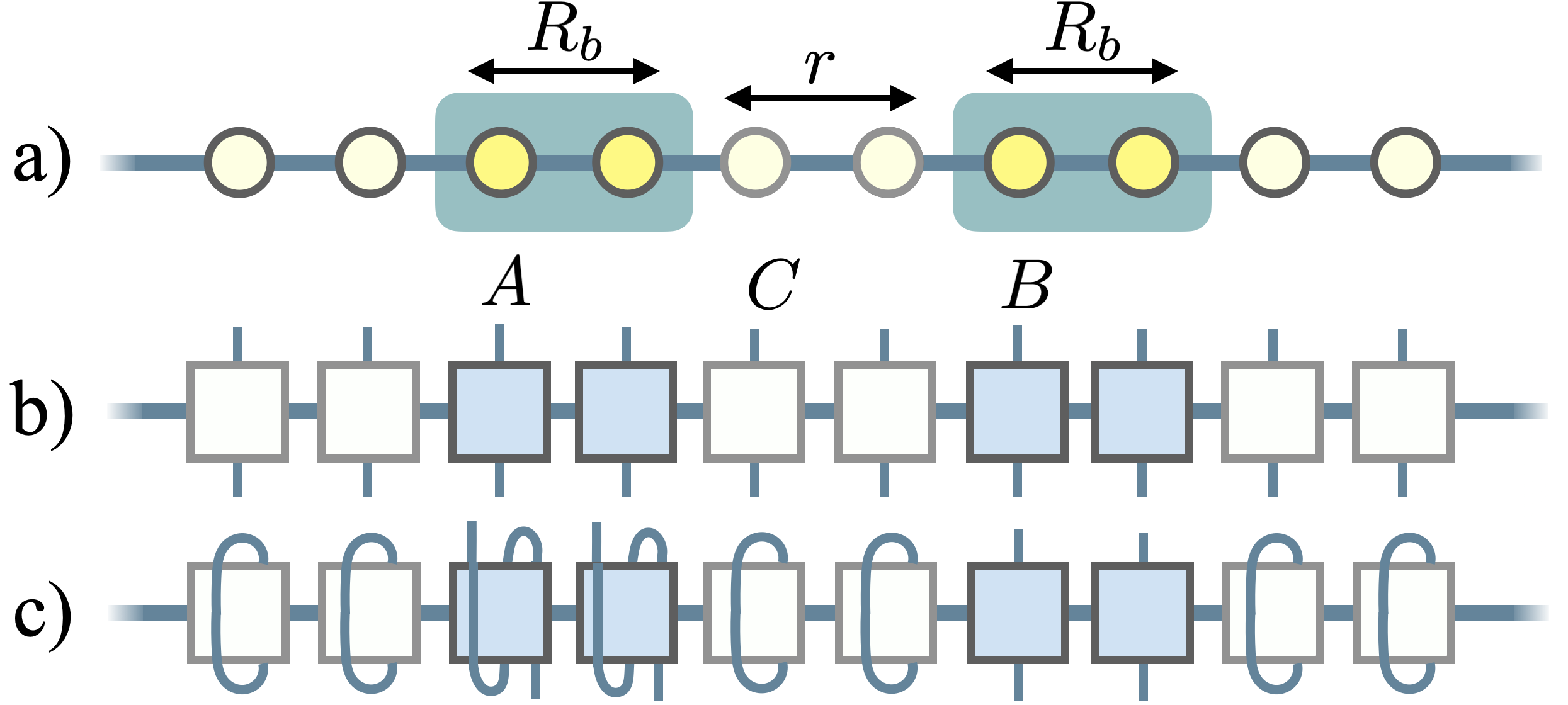
Fig. S7: Division into subsystems and computation of negativity: A sketch of how the entanglement negativity can be used to quantify the entanglement between subsystems of fixed size $R_{b}$ separated by a distance $r$. a) A sketch of the spin chain, identifying the subsystems $A$ and $B$ and the relevant distances $R_{b}$ and $r$. b) A sketch of the corresponding density matrix in MPO form, identifying the subsystems. c) A sketch of how the negativity is computed in this case, tracing out the complement of $A$ and $B$ while still applying the same ‘twist’ to the MPO legs in order to compute the partial transpose, as in Fig. 1 of the main text.

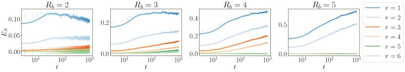
Fig. S8: Growth of negativity between subsystems of fixed size: Entanglement negativity following a quench from a Néel state, shown for disorder strength $d=6.0$ with system size $L=16$, averaged over $N_{s}=96$ disorder realisations. Here we compute the negativity for a subsystem of fixed size $R_{b}:=|A|=|B|$, as sketched in Fig. S7. We can see that for small values of $R_{b}$, the negativity at small separations $r$ saturates quickly and that only for larger values of $R_{b}$ does the negativity increase in a manner that allows extraction of the relevant $l$-bit length scale. Error bars show the standard error in the mean, and the solid lines are a smoothed guide to the eye.

Appendix G Supplementary note 6: Mutual information

In the main text and in our analytical results, we specified the logarithmic negativity as our chosen spatially-resolved entanglement probe. Here we briefly demonstrate that another spatially-resolved entanglement measure, the mutual information, also exhibits qualitatively similar behaviour. The mutual information between subsystems $A$ and $B$ is defined as

$$I(A:B):=S(\rho^{A})+S(\rho^{B})-S(\rho^{AB})$$ (9)

where $S(\rho):=-{\rm tr}\rho\log(\rho)$ represents the von Neumann entropy of a quantum state $\rho$, and $\rho^{A}$ is the reduced quantum state of subsystem $A$. Fig. S9 shows the results for a small system of size $L=12$ with bond dimension $\chi=128$, averaged over $N_{s}=100$ disorder realisations. The mutual information is qualitatively – and even quantitatively, in many cases – similar to the entanglement negativity, strongly suggesting that it would be a more than acceptable substitute and that much of the intuition developed in the main text should also apply to the mutual information. These findings are compatible with those using the multi-partite mutual information as a probe for many-body localization Goold et al. (2015); De Tomasi et al. (2017).

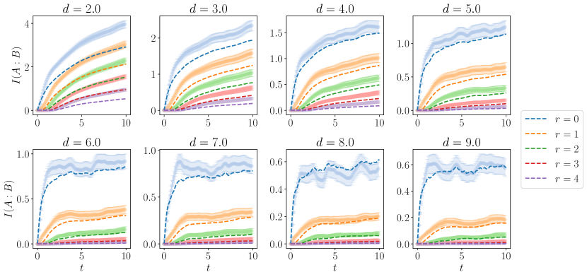
Fig. S9: Mutual information between separated regions over time: A comparison of mutual information (solid lines) and entanglement negativity (dashed lines) between subsystems $A$ and $B$ separated by a distance $r$, for a system of size $L=12$ with bond dimension $\chi=128$, averaged over $N_{s}=100$ disorder realisations.

Appendix H Supplementary note 7: Computation of the $l$-bits and the quasi-locality measure

The $l$-bits in this work are calculated using the method described in Ref. Goihl et al. (2018b). For completeness, we offer a brief explanation of the method: A system in the fully many-body localised phase can be fully characterized by a complete set of $l$-bits. Let $H$ be the MBL Hamiltonian of a system of size $N$ and $\tau_{i},\ i=1,\dots,N$, be the $l$-bits, then they need to satisfy the following properties:

1. $[H,\tau^{z}_{i}]=0$,

2. $[\tau^{z}_{i},\tau^{z}_{j}]=0$ for all $i$ and $j$,

3. $\tau_{i}$ is quasi-local in real space (will be elaborated in the next section).

A simple prescription in Ref. Kim et al. (2014) has been given to construct the $l$-bits out of infinite time averages of terms that the Hamiltonian contains. The infinite-time average of a term $h_{j}$ is

$$\mathbbm{E}(h_{j})=\lim_{T\rightarrow\infty}\frac{1}{T}\int_{0}^{T}e^{-iHt}\ h_{j}\ e^{iHt}\mathop{\mathrm{d}t}=\sum_{k}\bra{E_{k}}h_{j}\ket{E_{k}}\ket{E_{k}}\bra{E_{k}},$$ (10)

assuming a non-degenerate spectrum $\{E_{k}\}$ of $H$. Therefore, $\mathbbm{E}(h_{j})$, being sums of projectors onto the eigenstates of $H$, automatically fulfill properties 1 and 2. The authors have also demonstrated the quasi-locality of the resulting operator, showing that the non-local contributions from the off-diagonal elements, i.e., contributions from $\tau^{x}$ and $\tau^{y}$ will be removed through the infinite-time averaging procedure. The downside with this approach is that the resulting operator has a degenerate spectrum that is distinct from what the Pauli algebra mandates. Thus, we can no longer associate this operator with the picture of having ladder operators that help us transverse through the different modes/eigenstates.

The authors in Ref. Goihl et al. (2018b) have computed $\mathbb{E}(\sigma_{j}^{z})$ from (10) and re-arranged the order of the eigenstates in $U_{d}$ to minimize the pair-wise differences between the spectrum of $\mathbb{E}(\sigma_{j}^{z})$ and that of

$$\tau^{z}_{j}=U^{\dagger}_{d}\sigma^{z}_{j}U_{d},$$ (11)

starting with $j=1$ and sequentially optimising the eigenstate order with larger $j$ while keeping the already optimized partial ordering from smaller $j$ intact. The resulting operators will preserve the Pauli algebra by construction while becoming quasi-local in real space. For simplicity, we only deal with trace-less and Hermitian operators for the moment. Operators with non-vanishing traces require special procedures to meet the orthonormality of the Hilbert-Schmidt inner product.

Definition 3 (Quasi-locality).

Let $\tau$ be a trace-less Hermitian operator, normalized with respect to the Frobenius norm, and $L_{i}$ its orthogonal trace-less Hermitian basis. Consider the decomposition

$$\tau=\sum_{i}a_{i}L_{i}.$$ (12)

Let $S(L_{i})$ be the support of $L_{i}$ in real-space. $\tau$ is quasi-local around site $j$, if and only if for any connected region $B$ containing $j$, we have

$$\sum_{S(L_{i})\nsubseteq B}|{a_{i}}|^{2}\leq k\exp(-\text{dist}(j,B)/\xi).$$ (13)

This definition, although rigorous, can be cumbersome, and it is not easy to compute the relevant quantities. Let us consider the partial trace of the operator $\tau$,

$${\rm tr}_{B^{C}}(\tau)=2^{|{B^{C}}|}\sum_{S(L_{i})\subseteq B}a_{i}\tilde{L}_{i},$$ (14)

where $\tilde{L}_{i}$ are now defined on a smaller Hilbert space contained in $B$ and the extra identity operators outside $B$ become the pre-factor $2^{|{B^{C}}|}$ after the partial trace. Then, we can compute the square of the Frobenius norm of this truncated operator to get

$$\left\|{{\rm tr}_{B^{C}}(\tau)}\right\|^{2}_{2}=2^{2|{B^{C}}|}{\rm tr}(\sum_{S(L_{i})\subseteq B}a^{*}_{i}\tilde{L}_{i}\sum_{S(L_{j})\subseteq B}a_{j}\tilde{L}_{j})=2^{2|{B^{C}}|+|{B}|}\sum_{S(L_{i})\subseteq B}|{a_{i}}|^{2},$$ (15)

due to the orthogonality of the basis operators $L_{i}$ and their restrictions to any region $B$. Finally, we leverage the normalisation of $\tau$ to observe that

$$\sum_{S(L_{i})\subseteq B}|{a_{i}}|^{2}+\sum_{S(L_{i})\nsubseteq B}|{a_{i}}|^{2}=\left\|{\tau}\right\|^{2}_{2}=1.$$ (16)

Therefore,

$$\sum_{S(L_{i})\nsubseteq B}|{a_{i}}|^{2}=1-\frac{1}{2^{|{B}|+2|{B^{C}}|}}\left\|{{\rm tr}_{B^{C}}(\tau)}\right\|_{2}^{2}\leq k\exp(-\text{dist}(j,B)/\xi).$$ (17)

This is exactly the quasi-locality measure proposed in Refs. Goihl et al. (2018b); Chandran et al. (2015). The spatial decay of the $l$-bits can also be computed using the weight measure in Eq. (6) from Ref. Kulshreshtha et al. (2018). This notion of quasi-locality is agnostic to operator content and where it is quasi-local around because one only needs to compute the weight of the operator filtered at each site.

Appendix I Supplementary note 8: Entanglement growth bound

In this section, we prove an entanglement growth bound that has been tailored for the case at hand. Generic entanglement growth bounds for the entanglement entropy have been proven for local Hamiltonians Mariën et al. (2016); Eisert and Osborne (2006); Eisert (2021); Kim et al. (2014). Here, we prove novel bounds for the negativity, ones that are tailored to be applicable to many-body localised systems and the geometry at hand. We now look at the specific setting of having two regions, $A$ and $B$ separated by a region $C$ that has been traced out, and ask how much entanglement can be generated by a many-body localised Hamiltonian. We consider states evolving in time as $\rho(t):=e^{-itH}\rho e^{itH}$. For the purpose of this proof, we will consider a slightly strengthened definition of quasi-locality with respect to the definition in the main text, namely, instead of the normalized Frobenius norm, we will assume the $l$-bits are localised in the operator norm, i.e., the following.

Definition 4 (Strong quasi-locality).

An operator is said to be quasi-local around a region $R$, if for any region $X\subset R$, it holds that

$$\left\|O-\frac{1}{2^{|X^{c}|}}{\rm tr}_{X^{c}}(O)\otimes\mathbb{I}_{X_{c}}\right\|_{\infty}^{2}\leq\|O\|_{\infty}^{2}Ke^{-d(R,X^{c})/\xi}$$ (18)

for some constant $K>0$.

This definition is stronger than the definition in the main text, in the sense that if an operator is quasi-local in the sense above, it is also quasi-local in the sense of the main text. For convenience, we repeat here the definition of a many-body localized Hamiltonian:

Definition 5 (Many-body localisation).

A Hamiltonian

$$H=\sum_{j=1}^{n}\omega_{j}^{(1)}h_{j}+\sum_{j,k=1}^{n}\omega^{(2)}_{j,k}h_{j}h_{k}+\dots$$ (19)

with real weights $\{\omega_{j}^{(1)}\}$ and $\{\omega_{j,k}^{(2)}\}$, is called many-body localised if it can be written as a sum of mutually commuting ($[h_{j},h_{k}]=0$ for all $j,k$) quasi-local terms $h_{j}$, each centred around site $j$, and if $\omega_{i_{1},\dots,i_{n}}\leq\omega e^{-|i_{1}-i_{n}|/\kappa}$, where $i_{1}<i_{2}\dots<i_{n}$.

The following is the central statement from which the entanglement bound easily follows:

Theorem 2 (Entanglement growth bound for sums of quasi-local operators).

Let $\rho$ be any initial state. Let $H$ be a many-body localised Hamiltonian as per Definition 5 with localisation length $\xi\leq{1}/{(4\log(2))}$ and $2(1/\kappa-\log(2))>1/\xi$, consider three blocks $A,C,B$ such that $C$ divides $A$ from $B$ the growth of the negativity of the state $\rho(t)=e^{-itH}\rho e^{itH}$ restricted to the regions $A,B$ for times $t\geq 0$ and for any $r\geq|C|/2$

$$E_{N}(t)=\log_{2}(\|\rho_{A,B}^{T_{A}}(t)\|_{1})\leq 4r-2|C|+tO(e^{-r/(2\xi)}).$$ (20)

Notice the the $r$ in the above is a parameter one can choose freely. We obtain the following statement, morally, by picking $r=2\xi\log(t)$ in the above bound if $t>e^{|C|/(4\xi)}$ and $r=|C|/2$ otherwise. Some additional details are required in order not to consider a time dependent $r$ in the proof of Theorem 2.

Corollary 1.

[Logarithmic growth of the negativity] If $t\geq e^{|C|/{4\xi}}$, under the assumptions of Theorem 2, we have

$$E_{N}(t)\leq\mathchoice{\operatorname*{min}}{\operatorname*{min}}{\mathrm{min}}{\mathrm{min}}\{t\,O(e^{-|C|/(4\xi)}),8\xi\log(t)-2|C|\}+O(1),$$ (21)

while for $t<e^{|C|/{4\xi}}$,

$$E_{N}(t)\leq t\,O(e^{-|C|/(4\xi)})$$ (22)

Proof.

For the $t<e^{|C|/{4\xi}}$ case, one need only pick $r=|C|/2$. Otherwise, for any time $t$, let $r^{*}$ be the positive integer such that $e^{r^{*}/(2\xi)}\leq t\leq e^{(r^{*}+1)/(2\xi)}$. Then $r^{*}\leq 2\xi\log(t)\leq r^{*}+1$. Picking $r=r^{*}$ we get

$$E_{N}(t)=\leq 4r^{*}-2|C|+tO(e^{-r^{*}/(2\xi)})\leq 8\xi\log(t)-2|C|+O(t\,e^{\log(t)+1/(2\xi)})=8\xi\log(t)-2|C|+O(1),$$ (23)

since the bound with $r=|C|/2$ still holds, one can pick the minimum between these two bounds. ∎

To turn this result into a proper bound for many-body localised Hamiltonians, we need to reduce such Hamiltonians to the form considered in Theorem 2. For this purpose, we will assume a slightly stronger definition of the many-body localised Hamiltonian. We call a unitary quasi-local with localisation length $\xi$ if it maps any local operator on a region $R$ to a quasi-local operator around $R$ with localisation length $\xi$. We will assume that the Hamiltonian is diagonalised by a quasi-local unitary, which means that the $l$-bits are simply dressed Pauli $Z$ operators, $h_{i}=U\sigma_{z}^{i}U^{\dagger}$. In particular this implies that a product of $l$-bits $h_{i_{1}}h_{i_{2}}\dots h_{i_{n}}$, with $i_{1}<i_{2}<\dots<i_{n}$ is quasi-local around $\{i_{1},\dots,i_{n}\}$. For the purposes of the subsequent discussion, it will be useful to define the projector

$$\mathcal{P}_{X}(O)={\rm tr}_{X^{c}}(O)\otimes\frac{I}{2^{|X^{c}|}},$$ (24)

for any region $X$ of the lattice. It is easy to verify that $\mathcal{P}_{X}$ is a projector and that it is self-adjoint in the Hilbert Schmidt inner product. In what follows, $\|\cdot\|$ denotes the operator norm.

Lemma 1 (Quasi-local sums).

Let $H$ be a many-body localised Hamiltonian in the sense described above with localisation length $\xi$, and in addition, assume $2(1/\kappa-\log(2))>1/\xi$, where $\kappa$ has been defined in Definition 5. Then the Hamiltonian can be written as

$$H=\sum_{i=1}^{N}H_{i}$$ (25)

where $H_{i}$ is quasi-local around the site $i$ with localisation length $2\xi$.

We note that, a quasi-local operator with localisation length $\xi$ is quasi-local for any localisation length $\xi^{\prime}>\xi$, if $2(1/\kappa-\log(2))\leq 1/\xi$, it suffices to relax the quasi-locality of the $l$-bits by increasing the localisation length until this condition is satisfied, i.e., choose

$$\xi^{\prime}=\frac{1}{2(1/\kappa-\log(2))}+\epsilon>\xi$$ (26)

for some constant $\epsilon>0$. This will result in faster ($\sim r/\xi^{\prime})$, but still exponentially slow, growth of entanglement in the bound.

Proof.

Define $H_{i}$ as

$$H_{i}=\omega_{i}h_{i}+\sum_{l\geq 1}\sum_{k=2}^{2l+1}\sum_{I_{k}\in B_{k}(i,l)}\omega_{I_{k}}h_{I_{k}}$$ (27)

where $I_{k}=\{i_{1},\dots,i_{k}\}$ are collections of $k$ sites contained in $i-l\dots i+l$, containing the left boundary and either the right boundary or the site immediately to the left of it. We denote the set of all such $I_{k}$ as $B_{k}(i,l)$ (c.f. Figure S10).

Fig. S10: Examples of sets of sites contained in $B_{k}(i,l)$: In this example, $k=4$ and $l=3$. The sites $i$, $i+l$, $i-l$ are highlighted in red.

In the above, we have defined $h_{I_{k}}=h_{i_{1}}\dots h_{i_{k}}$. We have then $\omega_{I_{k}}^{2}\leq\omega^{2}e^{-(2l-1)/\kappa}$ and that $h_{I_{k}}$ is quasi-local around $[i-l,i+l]$ with localisation length $\xi$. We have $H=\sum_{i}H_{i}$, it remains to show that the $H_{i}$ are quasi-local as claimed. Let $R=[i-r,i+r]$ be a stretch of sites of radius $r$ around $i$. We have, by the triangle inequality,

$$\|H_{i}-\mathcal{P}_{R}(H_{i})\| =\omega_{i}\|h_{i}-\mathcal{P}_{R}(h_{i})\|+\sum_{l\geq 1}\sum_{k=2}^{2l+1}\sum_{I_{k}\in B_{k}(i,l)}\omega_{I_{k}}\|h_{i}-\mathcal{P}_{R}(h_{i})\|$$ (28)

$$\leq\omega Ke^{-r/\xi}+K\sum_{l=1}^{r-1}\sum_{I_{k}\in B_{k}(i,l)}\omega e^{-(2l-1)/\kappa}e^{-(r-l)/(2\xi)}+2\sum_{l\geq r}\sum_{I_{k}\in B_{k}(i,l)}\omega e^{-(2l-1)/\kappa},$$

where we have used quasi-locality and in the $l\geq r$ part of the sum, that $\|h_{i}-\mathcal{P}_{R}(h_{i})\|\leq 2$. Now notice that

$$\sum_{I_{k}\in B_{k}(i,l)}=2\cdot 2^{2l-2}=2^{2l-1}\leq 2^{2l},$$ (29)

we then have that

$$\|H_{i}-\mathcal{P}_{R}(H_{i})\| \leq\omega Ke^{-r/(2\xi)}+K\sum_{l=1}^{r-1}2^{2l}\omega e^{-2l/\kappa}e^{-(r-l)/(2\xi)}+2\sum_{l\geq r}2^{2l}\omega e^{-2l/\kappa}$$ (30)

$$=\omega Ke^{-r/(2\xi)}+K\sum_{l=1}^{r-1}\omega e^{-2l(1/\kappa-\log(2))}e^{-(r-l)/(2\xi)}+2\omega\sum_{l\geq r}e^{-2l(1/\kappa-\log(2))}.$$

The first term is already bounded as needed, and for the third term, we use $2(1/\kappa-\log(2))>1/(2\xi)$, to get

$$\sum_{l\geq r}e^{-2l(1/\kappa-\log(2))}\leq\sum_{l\geq r}e^{-l/(2\xi)}=\frac{1}{1-e^{-1/(2\xi)}}e^{-r/(2\xi)}.$$ (31)

For the second term, let $\delta=2(1/\kappa-\log(2))-1/(2\xi)>0$. Then

$$\sum_{l=1}^{r-1}e^{-2l(1/\kappa-\log(2))}e^{-(r-l)/(2\xi)}=e^{-r/(2\xi)}\sum_{l=1}^{r-1}e^{-\delta l}\leq\frac{e^{-\delta}}{1-e^{-\delta}}e^{-r/(2\xi)}.$$ (32)

We note in passing that if $\delta=0$, the bound does not diverge, but an additional linear term is added to get a bound of the form $re^{-r\xi}$. In conclusion,

$$\|H_{i}-\mathcal{P}_{R}(H_{i})\|\leq K^{\prime}e^{-r/(2\xi)}$$ (33)

with

$$K^{\prime}:=\omega\left(K+K\frac{e^{-\delta}}{1-e^{-\delta}}+\frac{2}{1-e^{-1/\xi}}\right),$$ (34)

that is,

$$\|H_{i}-\mathcal{P}_{R}(H_{i})\|^{2}\leq K^{\prime 2}e^{-r/\xi}$$ (35)

which is the definition of quasi-locality noticing $||h_{i}||=1$. ∎

The rest of this section is dedicated to proving Theorem 2. The technique used for the proof is analogous to that of Ref. Kim et al. (2014), where an analogous bound was derived for the entanglement entropy in the case $|C|=0$, the properties of the negativity, which is a meaningful entanglement measure for mixed states, allow the generalisation to disconnected regions. The following two properties of the $1$-norm and the partial transpose will be used repeatedly:

• The $1-$norm contracts under the partial trace, i.e., $||\rho_{A}||_{1}\leq||\rho_{A,B}||_{1}$ for any bipartite state $\rho_{A,B}$ Rastegin (2012),

• $||\rho_{A,B}^{T_{B}}||_{1}\leq d_{B}||\rho_{A,B}||_{1}$ Tsuyoshi and Sano (2008).

We will now prove Theorem 2. From now on we will assume that $|C|$ is even, the odd case is analogous. We will label the two central sites of $C$ as $\pm 1$, all the sites to the right of the center of $C$ have positive integer labels, and to the left negative integer labels (notice that there is no site $0$). In addition, we will use the standard notation $[a,b)$ denoting real intervals to denote intervals in the chain, so from now on $[a,b)$ is understood to mean $[a,b)\cap\mathbb{Z}/\{0\}$.

Divide the chain into the following regions (see Fig. S11), recall that $r$ is an arbitrary integer greater than $|C|/2$.

$$\bar{L}=(-\infty,-r+|C|/2),\quad L=(-\infty,|C|/2),$$ (36)

$$\bar{\mathop{}}\!\partial=[-r+|C|/2,r-|C|/2],\quad\mathop{}\!\partial=[-2r+|C|/2,2r-|C|/2],$$ (37)

$$\bar{R}=(r-|C|/2,\infty),\quad R=(-|C|/2,\infty),$$ (38)

and divide the terms in the Hamiltonian accordingly as

$$H=h_{\bar{L}}+h_{\bar{R}}+h_{\bar{\mathop{}}\!\partial}$$ (39)

where $h_{\bar{S}}=\sum_{i\in S}h_{i}$ for $S\in{L,\mathop{}\!\partial,R}$. We will now split the term $h_{\bar{S}}$ into a main local part acting on $S$ and a tail whose norm is exponentially small in $r$.

Fig. S11: Division of the chain into regions for the proof of Theorem 2: The central region bounded by the vertical lines is $C$, represented by the dashed red and blue line. Note that $C$ is contained in both $L$ and $R$.

More specifically, we can isolate the tail evolution as follows

Lemma 2.

Let $H_{S}=\mathcal{P}_{S}(h_{\bar{S}})$ and define the corresponding tail as $T_{S}=h_{\bar{S}}-H_{S}$, then

$$e^{ih_{\bar{S}}t}=e^{iH_{S}t}U^{T}_{S}(t)$$ (40)

where the tail evolution is given by

$$U_{S}^{T}(t)=\mathcal{T}\left(\exp\left(\int_{0}^{t}\mathrm{d}\tau\,\tilde{T}_{S}(\tau)\right)\right)=\sum_{k=0}^{\infty}i^{k}\int_{0}^{t}\mathrm{d}t_{1}\,\dots\int_{0}^{t_{k-1}}\mathrm{d}t_{k}\tilde{T}_{S}(t_{1})\dots\tilde{T}_{S}(t_{k})$$ (41)

where

$$\tilde{T}_{S}(\tau)=e^{-iH_{S}\tau}T_{S}e^{iH_{S}\tau}.$$ (42)

Proof.

We have $U^{T}_{S}(t)=e^{-iH_{S}t}e^{ih_{S}t}$, hence

$$\frac{\mathrm{d}}{\mathrm{d}t}U^{T}_{S}(t)=-iH_{S}e^{-iH_{S}t}e^{ih_{\bar{S}}t}+ie^{-iH_{S}t}h_{S}e^{ih_{\bar{S}}t}=ie^{-iH_{S}t}Te^{ih_{\bar{S}}t}=\tilde{T}_{S}(t)U^{T}_{S}(t)$$ (43)

this is the differential equation satisfied by the time evolution operator with the time-dependent Hamiltonian $\tilde{T}_{S}(t)$, it is well known that its solution is given by the Dyson series in the statement. ∎

Notice that the tail evolution is an operator acting globally on the lattice, hence it could still, in principle, create an amount of entanglement extensive in the system size. The intuition is that it is generated by $\tilde{T}_{S}$, which has exponentially small norm. We need to formalize the idea that this leftover tail evolution cannot create much entanglement. For each $S$, define $S+q$ as the region $S$ extended to the left and the right (if possible) by $q$ sites. We can then write the tail $T_{S}$ as a telescopic sum, defining $H_{S+q}=\mathcal{P}_{S+q}(h_{\bar{S}})$

$$T_{S}=-H_{S}+H_{S+1}-H_{S+1}+H_{S+2}-H_{S+2}\dots=-\sum_{q=0}^{\infty}H_{S+q}-H_{S+q+1}.$$ (44)

Clearly $h_{\bar{S}}=\lim_{q\to\infty}\mathcal{P}_{S+q}(h_{\bar{S}})$, as this is simply the “truncation” where the whole lattice is kept. We then have that

$$T_{S}=\sum_{q=0}^{\infty}Z_{S+q+1}$$ (45)

where $Z_{S+q}:=H_{S+q}-H_{S+q+1}$ acts only on $S+q+1$. Until now, we have claimed that these tail operators have exponentially small norms in $r$. Before continuing, let us prove this.

Lemma 3 (Tail bounds).

$||Z_{S+q}||\leq O(e^{-(r+q)/(2\xi)})$.

Proof.

We will prove that $||h_{\bar{S}}-H_{S+q}||\leq O(e^{-(r+q)/(2\xi)})$, the statement follows as

$$||Z_{S+q}||\leq||H_{S+q}-H_{S+q+1}||\leq(||H_{S+q}-h_{\bar{S}}||+||H_{S+q+1}-h_{\bar{S}}||).$$ (46)

Let us start with $S=\mathop{}\!\partial$. The closest $l$-bits to the boundary of $\mathop{}\!\partial+q$ in $\bar{\mathop{}}\!\partial$ are separated from it by $r+q$ sites, and the furthest ones by $2r+q$. The sum is clearly symmetric around the centre of the chain, and we use that for any $S$, $S$ is constructed such that the distance from any site in $\bar{S}$ to the edge of $\bar{S}$ is at least $r$. Recall that $h_{\bar{S}}=\sum_{i\in\bar{S}}h_{i}$, where the $h_{i}$ are quasi-local as in Definition 4, so that

$$||h_{\bar{\mathop{}\!\partial}}-H_{\mathop{}\!\partial+q}||\leq\sum_{k=-r+|C|/2}^{r-|C|/2}||h_{k}-\mathcal{P}_{\mathop{}\!\partial+q}(h_{k})||\leq 2K\sum_{j=r+q}^{2r+q-|C|/2}e^{-j/(2\xi)}\leq O(e^{-(r+q)/(2\xi)})$$ (47)

for some constant $K>0$, by the definition of quasi-locality. Let us move to $S=R$, where again the closest l-bits in $\bar{R}$ to the boundary of $R+q$ are separated from it by $r+q$ sites, and the furthest has a distance unbounded in the system size. We have

$$||h_{\bar{R}}-H_{R+q}||\leq\sum_{k>r-|C|/2}||h_{k}-\mathcal{P}_{R+q}(h_{k})||\leq 2K\sum_{j\geq r+q}e^{-j/(2\xi)}\leq O(e^{-(r+q)/(2\xi)}).$$ (48)

$S=L$ can be treated entirely analogously. ∎

We have completed the split into local terms and tails. The intuition is now that the entanglement in the system will be driven on the one hand by the term $H_{\mathop{}\!\partial}$, which is the only local term connecting $A$ and $B$, and on the other hand by the tail. The former can only create entanglement locally around $C$, and the latter is weak. Next, we need to formalize the notion that the tails can only create weak entanglement.

Lemma 4 (Tails create weak entanglement.).

Let $R$ be any region of the chain, then

$$||(U_{S}(t)\rho(U_{S}^{T}(t))^{\dagger})^{T_{R}}||_{1}\leq O\left(\exp\left(2e^{-r/(2\xi)}C_{R,S}t\right)\right)||\rho^{T_{R}}||_{1}$$ (49)

with $C_{R,S}=\sum_{q=0}^{\infty}e^{-q/(2\xi)}d_{R\cap(S+q)}^{2}$.

We note in passing that clearly this bound is non trivial only if the constant $C_{R,S}$ is finite.

Proof.

First, notice the following fact. For any region $R$, operator $O$, and local operator $Z_{I}$ on a region $I$, we have

$$\|(Z_{I}O)^{T_{R}}\|_{1}\leq d_{R\cap I}\|Z_{I}O^{T_{R/I}}\|_{1}\leq d_{R\cap I}\|Z_{I}\|\|O^{T_{R/I}}\|_{1}=d_{R\cap I}\|Z_{I}\|\|(O^{T_{R}})^{T_{R\cap I}}\|_{1}\leq d_{R\cap I}^{2}\|Z_{I}\|\|O^{T_{R}}\|_{1}$$ (50)

next, we use the Dyson series expression for the tail evolution. First, notice that by the triangle inequality

$$||(U_{S}(t)\rho(U_{S}^{T}(t))^{\dagger})^{T_{R}}||_{1}\leq\sum_{k,n=0}^{\infty}\int_{0}^{t}\mathrm{d}t_{1}\dots\int_{0}^{t_{k-1}}\mathrm{d}t_{k}\int_{0}^{t}\mathrm{d}s_{1}\dots\int_{0}^{s_{n-1}}\mathrm{d}s_{n}\left\|\left(\tilde{T}_{S}(t_{1})\dots\tilde{T}_{S}(t_{k})\rho\tilde{T}_{S}(s_{n})\dots\tilde{T}_{S}(s_{1})\right)^{T_{R}}\right\|_{1}$$ (51)

recall that we can write

$$\tilde{T}_{S}(t)=\sum_{q=0}^{\infty}\tilde{Z}_{S+q}(t)$$ (52)

where $\tilde{Z}_{S+q}(t)=e^{-iH_{S}t}Z_{S+q}e^{iH_{S}t}$ acts only on $S+q$. We then have, using Eq.  (50) and the triangle inequality

$$\left\|\left(\tilde{T}_{S}(t_{1})\dots\tilde{T}_{S}(t_{k})\rho\tilde{T}_{S}(s_{n})\dots\tilde{T}_{S}(s_{1})\right)^{T_{R}}\right\|_{1}\leq$$ (53)

$$\sum_{\begin{subarray}{c}q_{1},\dots,q_{k}=0\\ p_{1},\dots,p_{n}=0\end{subarray}}^{\infty}\left\|\left(\tilde{Z}_{S+q_{1}}(t_{1})\dots\tilde{Z}_{S+q_{k}}(t_{k})\rho\tilde{Z}_{S+p_{n}}(s_{n})\dots\tilde{Z}_{S+p_{1}}(s_{1})\right)^{T_{R}}\right\|_{1}\leq||\rho^{T_{R}}||_{1}\left(\sum_{q=0}^{\infty}||Z_{S+q}||d_{R\cap(S+q)}^{2}\right)^{n+k}$$

before plugging this in in the initial expression, notice that

$$\int_{0}^{t}\mathrm{d}t_{1}\dots\int_{0}^{t_{k-1}}\mathrm{d}t_{k}=\frac{t^{k}}{k!},$$ (54)

we then have

$$||(U_{S}^{T}(t)\rho(U_{S}^{T}(t))^{\dagger})^{T_{R}}||_{1}\leq\sum_{k,n=0}^{\infty}\frac{t^{k}}{k!}\frac{t^{n}}{n!}\left(\sum_{q=0}^{\infty}||Z_{S+q}||d_{R\cap(S+q)}^{2}\right)^{n+k}=\exp\left(2t\sum_{q=0}^{\infty}||Z_{S+q}||d_{R\cap(S+q)}^{2}\right).$$ (55)

We can conclude by using that by Lemma 3 that this expression has a norm bounded by $\|\tilde{Z}_{S+q}(t)\|=\|Z_{S+q}\|\leq O\left(e^{-(r+q)/(2\xi)}\right)$. ∎

This allows us to prove the first part of the bound: We can write

$$e^{iHt}=e^{iH_{\mathop{}\!\partial}t}U^{T}_{\mathop{}\!\partial}(t)e^{iH_{L}t}U^{T}_{L}(t)e^{iH_{R}t}U^{T}_{R}(t).$$ (56)

Given a generator $h$, define the evolution operator $\mathcal{U}_{h}(\rho):=e^{ih}\rho e^{-ih}$, furthermore define the tail evolution operator as $\mathcal{U}^{T,t}_{S}(\rho)=U^{T}(t)_{S}\rho(U^{T}(t)_{S})^{\dagger}$. Consider a state $\sigma$, notice that the overlap between $B$ and $\mathop{}\!\partial$ is of length $2r-|C|$, in particular,

$$||{\rm tr}_{C}(\mathcal{U}_{H_{\mathop{}\!\partial}t}(\sigma))^{T_{B}}||_{1}\leq||{\rm tr}_{C}(e^{iH_{\mathop{}\!\partial}t}(\sigma)^{T_{(2r-|C|/2,\infty)}}e^{-iH_{\mathop{}\!\partial}t})^{T_{[|C|/2,2r-|C|/2]}}||_{1}\leq 2^{2r-|C|}||\sigma^{T_{(2r-|C|/2,\infty)}}||_{1}$$ (57)

Here, we simply assume sufficient time has passed that $H_{\mathop{}\!\partial}$ has had time to saturate the entanglement in the region $\mathop{}\!\partial$, that is, create a maximally entangled state between the sites on either side of $C$. We have then

$$||\rho(t)^{T_{B}}||_{1} =\left\|{\rm tr}_{C}\left(\mathcal{U}_{H_{\mathop{}\!\partial}t}\circ\mathcal{U}_{\mathop{}\!\partial}^{T,t}\circ\mathcal{U}_{{H_{L}}t}\circ\mathcal{U}_{L}^{T,t}\circ\mathcal{U}_{H_{R}t}\circ\mathcal{U}_{R}^{T,t}(\rho)\right)^{T_{B}}\right\|_{1}$$ (58)

$$\leq 2^{2r-|C|}\left\|\left(\mathcal{U}_{\mathop{}\!\partial}^{T,t}\circ\mathcal{U}_{{H_{L}}t}\circ\mathcal{U}_{L}^{T,t}\circ\mathcal{U}_{H_{R}t}\circ\mathcal{U}_{R}^{T,t}(\rho)\right)^{T_{(2r-|C|/2,\infty)}}\right\|_{1}.$$

Next, by Lemma 4, we have

$$\left\|\rho(t)^{T_{B}}\right\|_{1} \leq 2^{2r-|C|}E_{\mathop{}\!\partial,t}\left\|\left(\mathcal{U}_{{H_{L}}t}\circ\mathcal{U}_{L}^{T,t}\circ\mathcal{U}_{H_{R}t}\circ\mathcal{U}_{R}^{T,t}(\rho)\right)^{T_{(2r-|C|/2,\infty)}}\right\|_{1}$$ (59)

where

$$E_{\mathop{}\!\partial,t} \leq\exp\left(tO\left(e^{-r/(2\xi)}\sum_{q=0}^{\infty}2^{2(|\mathop{}\!\partial+q+1\cap(2r-|C|/2,\infty)|)}e^{-q/(2\xi)}\right)\right)$$ (60)

$$\leq\exp\left(tO\left(e^{-r/(2\xi)}\sum_{q=0}^{\infty}2^{2q}e^{-q/(2\xi)}\right)\right)\leq\exp\left(tO\left(e^{-r/(2\xi)}\right)\right),$$

where we have used the assumption $\xi<{1}/({4\log(2)})$, so that the terms in the sum above are exponentially decaying and sum to a constant. Since $L$ has no overlap with $(2r-|C|/2,\infty)$, we can just bring the partial transpose inside the $L$ evolution and eliminate it by unitarity. Afterwards, we eliminate $\mathcal{U}_{L}^{T,t}$, exactly as we have eliminated $\mathcal{U}_{\mathop{}\!\partial}^{T,t}$, to get

$$||\rho(t)^{T_{B}}||_{1} =2^{2r-|C|}E_{\mathop{}\!\partial,t}E_{L,t}\left\|\left(\mathcal{U}_{H_{R}t}\circ\mathcal{U}_{R}^{T,t}(\rho)\right)^{T_{(2r-|C|/2,\infty)}}\right\|_{1}$$ (61)

and in the same way one can show that $E_{L,t}\leq\exp\left(t\,O\left(e^{-r/(2\xi)}\right)\right)$. Finally, notice that for any region $X$ and a state $\sigma$, $||\sigma^{T_{X}}||_{1}=||\sigma^{T_{X^{c}}}||_{1}$, since $\sigma$ is Hermitian. Then

$$\left\|\left(\mathcal{U}_{H_{R}t}\circ\mathcal{U}_{R}^{T,t}(\rho)\right)^{T_{(2r-|C|/2,\infty)}}\right\|_{1} =\left\|\left(\mathcal{U}_{H_{R}t}\circ\mathcal{U}_{R}^{T,t}(\rho)\right)^{T_{(-\infty,2r-|C|/2)}}\right\|_{1}$$ (62)

$$\leq 2^{2r-|C|}\left\|\left(\mathcal{U}_{R}^{T,t}(\rho)\right)^{T_{(-\infty,-|C|/2)}}\right\|_{1}\leq 2^{2r-|C|}E_{R,t}\left\|\rho^{T_{(-\infty,-|C|/2)}}\right\|_{1}$$

$$=2^{2r-|C|}E_{R,t},$$

where we have used that the initial state is a product state, $E_{R,t}$ can be bounded as in the previous cases. Overall, we have then proven that

$$||\rho(t)^{T_{B}}||_{1}\leq 2^{4r-2|C|}\exp\left(t\,O\left(e^{-r/(2\xi)}\right)\right)$$ (63)

holds true. The final result is obtained by applying $\log_{2}$ on both sides. Recall that the final bound for the growth in time of the logarithmic negativity is obtained by substituting $r\sim\log(t)$ when appropriate, see Corollary 1.

References

- Polkovnikov et al. (2011) A. Polkovnikov, K. Sengupta, A. Silva, and M. Vengalattore, “Non-equilibrium dynamics of closed interacting quantum systems,” Rev. Mod. Phys. 83, 863 (2011).
- Gogolin and Eisert (2016) C. Gogolin and J. Eisert, “Equilibration, thermalisation, and the emergence of statistical mechanics in closed quantum systems,” Rep. Prog. Phys. 79, 56001 (2016).
- Anderson (1958) P. W. Anderson, “Absence of diffusion in certain random lattices,” Phys. Rev. 109, 1492–1505 (1958).
- Fleishman and Anderson (1980) L. Fleishman and P. W. Anderson, “Interactions and the Anderson transition,” Phys. Rev. B 21, 2366–2377 (1980).
- Basko et al. (2006) D. M. Basko, I.L. Aleiner, and B.L. Altshuler, “Metal–insulator transition in a weakly interacting many-electron system with localized single-particle states,” Ann. Phys. 321, 1126–1205 (2006).
- Huse et al. (2013) D. A. Huse, R. Nandkishore, V. Oganesyan, A. Pal, and S. L. Sondhi, “Localization-protected quantum order,” Phys. Rev. B 88, 014206 (2013).
- Huse et al. (2014) D. A. Huse, R. Nandkishore, and V. Oganesyan, “Phenomenology of fully many-body-localized systems,” Phys. Rev. B 90, 174202 (2014).
- Altman and Vosk (2015) E. Altman and R. Vosk, “Universal dynamics and renormalization in many-body-localized systems,” Ann. Rev. Cond. Matt. Phys. 6, 383–409 (2015).
- Luitz et al. (2015) D. J. Luitz, N. Laflorencie, and F. Alet, “Many-body localization edge in the random-field Heisenberg chain,” Phys. Rev. B 91, 081103 (2015).
- Alet and Laflorencie (2018) F. Alet and N. Laflorencie, “Many-body localization: An introduction and selected topics,” Compt. Rend. Phys. 19, 498–525 (2018).
- Abanin et al. (2019) D. A. Abanin, E. Altman, I. Bloch, and M. Serbyn, “Colloquium: Many-body localization, thermalization, and entanglement,” Rev. Mod. Phys. 91, 021001 (2019).
- Friesdorf et al. (2015) M. Friesdorf, A. H. Werner, W. Brown, V. B. Scholz, and J. Eisert, “Many-body localisation implies that eigenvectors are matrix-product states,” Phys. Rev. Lett. 114, 170505 (2015).
- Serbyn et al. (2013) M. Serbyn, Z. Papić, and D. A. Abanin, “Local conservation laws and the structure of the many-body localized states,” Phys. Rev. Lett. 111, 127201 (2013).
- Ros et al. (2015) V. Ros, M. Müller, and A. Scardicchio, “Integrals of motion in the many-body localized phase,” Nucl. Phys. B 891, 420–465 (2015).
- Imbrie et al. (2017) J. Z. Imbrie, V. Ros, and A. Scardicchio, “Local integrals of motion in many-body localized systems,” Ann. Phys. 529, 1600278 (2017).
- Rademaker and Ortuño (2016) L. Rademaker and M. Ortuño, “Explicit local integrals of motion for the many-body localized state,” Phys. Rev. Lett. 116, 010404 (2016).
- Rademaker et al. (2017) L. Rademaker, M. Ortuño, and A. M. Somoza, “Many-body localization from the perspective of integrals of motion,” Ann. Phys. , 1600322 (2017).
- Pekker et al. (2017) D. Pekker, B. K. Clark, V. Oganesyan, and G. Refael, “Fixed points of Wegner-Wilson flows and many-body localization,” Phys. Rev. Lett. 119, 075701 (2017).
- Goihl et al. (2018a) M. Goihl, M. Gluza, C. Krumnow, and J. Eisert, “Construction of exact constants of motion and effective models for many-body localized systems,” Phys. Rev. B 97, 134202 (2018a).
- Thomson and Schiró (2018) S. J. Thomson and M. Schiró, “Time evolution of many-body localized systems with the flow equation approach,” Phys. Rev. B 97, 060201 (2018).
- Kulshreshtha et al. (2019) A. K. Kulshreshtha, A. Pal, T. B. Wahl, and S. H. Simon, “Approximating observables on eigenstates of large many-body localized systems,” Phys. Rev. B 99, 104201 (2019).
- Thomson and Schiró (2020) S. J. Thomson and M. Schiró, “Quasi-many-body localization of interacting fermions with long-range couplings,” Phys. Rev. Research 2, 043368 (2020).
- Thomson et al. (2021) S. J. Thomson, D. Magano, and M. Schiró, “Flow equations for disordered Floquet systems,” SciPost Phys. 11, 28 (2021).
- Thomson and Schirò (2023) S. J. Thomson and M. Schirò, “Local integrals of motion in quasiperiodic many-body localized systems,” SciPost Physics 14, 125 (2023).
- Thomson (2023) S. J. Thomson, “Disorder-induced spin-charge separation in the one-dimensional Hubbard model,” Phys. Rev. B 107 (2023), 10.1103/physrevb.107.l180201.
- Bertoni et al. (2022) C Bertoni, J Eisert, A Kshetrimayum, A Nietner, and S. J. Thomson, “Local integrals of motion and the stability of many-body localisation in disorder-free systems,” arXiv:2208.14432 (2022).
- Billy et al. (2008) J. Billy, V. Josse, Z. Zuo, A. Bernard, B. Hambrecht, P. Lugan, D. Clément, L. Sanchez-Palencia, P. Bouyer, and A. Aspect, “Direct observation of anderson localization of matter waves in a controlled disorder,” Nature 453, 891 (2008).
- Lukin et al. (2019) A. Lukin, M. Rispoli, R. Schittko, M. E. Tai, A. M. Kaufman, S. Choi, V. Khemani, J. Léonard, and M. Greiner, “Probing entanglement in a many-body–localized system,” Science 364, 256–260 (2019).
- Goihl et al. (2019) M. Goihl, M. Friesdorf, A. H. Werner, W. Brown, and J. Eisert, “Experimentally accessible witnesses of many-body localisation,” Quantum Rep. 1, 50 (2019).
- Chiaro et al. (2022) B. Chiaro, C. Neill, A. Bohrdt, M. Filippone, F. Arute, K. Arya, R. Babbush, D. Bacon, J. Bardin, R. Barends, S. Boixo, D. Buell, B. Burkett, Y. Chen, Z. Chen, R. Collins, A. Dunsworth, E. Farhi, A. Fowler, B. Foxen, C. Gidney, M. Giustina, M. Harrigan, T. Huang, S. Isakov, E. Jeffrey, Z. Jiang, D. Kafri, K. Kechedzhi, J. Kelly, P. Klimov, A. Korotkov, F. Kostritsa, D. Landhuis, E. Lucero, J. McClean, X. Mi, A. Megrant, M. Mohseni, J. Mutus, M. McEwen, O. Naaman, M. Neeley, M. Niu, A. Petukhov, C. Quintana, N. Rubin, D. Sank, K. Satzinger, T. White, Z. Yao, P. Yeh, A. Zalcman, V. Smelyanskiy, H. Neven, S. Gopalakrishnan, D. Abanin, M. Knap, J. Martinis, and P. Roushan, “Direct measurement of nonlocal interactions in the many-body localized phase,” Phys. Rev. Research 4, 013148 (2022).
- Goihl et al. (2018b) M. Goihl, M. Gluza, C. Krumnow, and J. Eisert, “Construction of exact constants of motion and effective models for many-body localized systems,” Phys. Rev. B 97, 134202 (2018b).
- Ilievski et al. (2016) E. Ilievski, M. Medenjak, T. Prosen, and L. Zadnik, “Quasilocal charges in integrable lattice systems,” J. Stat. Mech. , 064008 (2016).
- Chandran et al. (2015) A. Chandran, I. H. Kim, G. Vidal, and D. A. Abanin, “Constructing local integrals of motion in the many-body localized phase,” Phys. Rev. B 91, 085425 (2015).
- Doggen et al. (2018) E. V. H. Doggen, F. Schindler, K. S. Tikhonov, A. D. Mirlin, T. Neupert, D. G. Polyakov, and I. V. Gornyi, “Many-body localization and delocalization in large quantum chains,” Phys. Rev. B 98, 174202 (2018).
- Šuntajs et al. (2020a) Jan Šuntajs, J. Bonča, T. Prosen, and L. Vidmar, “Quantum chaos challenges many-body localization,” Phys. Rev. E 102, 062144 (2020a).
- Šuntajs et al. (2020b) J. Šuntajs, J. Bonča, T. Prosen, and L. Vidmar, “Ergodicity breaking transition in finite disordered spin chains,” Phys. Rev. B 102, 064207 (2020b).
- Sels and Polkovnikov (2023) D. Sels and A. Polkovnikov, “Thermalization of dilute impurities in one-dimensional spin chains,” Phys. Rev. X 13, 011041 (2023).
- Sels and Polkovnikov (2021) D. Sels and A. Polkovnikov, “Dynamical obstruction to localization in a disordered spin chain,” Phys. Rev. E 104, 054105 (2021).
- Bardarson et al. (2012) J. H. Bardarson, F. Pollmann, and J. E. Moore, “Unbounded growth of entanglement in models of many-body localization,” Phys. Rev. Lett. 109, 017202 (2012).
- Znidaric et al. (2008) M. Znidaric, T. Prosen, and P. Prelovsek, “Many-body localization in the Heisenberg XXZ magnet in a random field,” Phys. Rev. B 77, 064426 (2008).
- Życzkowski et al. (1998) K. Życzkowski, P. Horodecki, A. Sanpera, and M. Lewenstein, “Volume of the set of separable states,” Phys. Rev. A 58, 883–892 (1998).
- Eisert and Plenio (1999) J. Eisert and M. B. Plenio, “A comparison of entanglement measures,” J. Mod. Opt. 46, 145 (1999).
- Vidal and Werner (2002) G. Vidal and R. F. Werner, “Computable measure of entanglement,” Phys. Rev. A 65, 032314 (2002).
- Plenio (2005) M. B. Plenio, “Logarithmic negativity: A full entanglement monotone that is not convex,” Phys. Rev. Lett. 95, 090503 (2005).
- Eisert (2001) J. Eisert, “Entanglement in quantum information theory,” (2001), PhD thesis, University of Potsdam, arXiv:quant-ph/0610253.
- Ruggiero et al. (2016) P. Ruggiero, V. Alba, and P. Calabrese, “Entanglement negativity in random spin chains,” Phys. Rev. B 94, 035152 (2016).
- Ruggiero and Turkeshi (2022) P. Ruggiero and X. Turkeshi, “Quantum information spreading in random spin chains,” Phys. Rev. B 106, 134205 (2022).
- Gray et al. (2019) J. Gray, A. Bayat, A. Pal, and S. Bose, “Scale invariant entanglement negativity at the many-body localization transition,” arXiv:1908.02761 (2019).
- Gruber and Eisler (2020) M. Gruber and V. Eisler, “Time evolution of entanglement negativity across a defect,” J. Phys. A 53, 205301 (2020).
- Kim et al. (2014) I. H. Kim, A. Chandran, and D. A. Abanin, “Local integrals of motion and the logarithmic lightcone in many-body localized systems,” arXiv:1412.3073 (2014).
- (51) See Supplemental Material for details. The Supplemental Material contains Refs. Kulshreshtha et al. (2018); Mariën et al. (2016); Eisert and Osborne (2006); Eisert (2021); Rastegin (2012); Tsuyoshi and Sano (2008); Goold et al. (2015); De Tomasi et al. (2017).
- Lee and Ramakrishnan (1985) P. A. Lee and T. V. Ramakrishnan, “Disordered electronic systems,” Rev. Mod. Phys. 57, 287–337 (1985).
- Orús (2014) R. Orús, “A practical introduction to tensor networks: Matrix product states and projected entangled pair states,” Ann. Phys. 349, 117–158 (2014).
- Gray (2018a) J. Gray, “QUIMB: A python package for quantum information and many-body calculations,” J. Open Source Soft. 3, 819 (2018a).
- Vidal (2004) G. Vidal, “Efficient simulation of one-dimensional quantum many-body systems,” Phys. Rev. Lett. 93, 040502 (2004).
- Schollwöck (2011) U. Schollwöck, “The density-matrix renormalization group in the age of matrix product states,” Ann. Phys. 326, 96 (2011).
- Gray (2018b) J. Gray, “Fast computation of many-body entanglement,” arXiv:1809.01685 (2018b).
- Lu et al. (2022) B. Lu, C. Bertoni, S. J. Thomson, and J. Eisert, https://doi.org/10.5281/zenodo.7322988 (2022).
- Thomson (2022) S. J. Thomson, https://github.com/sjt48/EntanglementDynamics (2022).
- Goold et al. (2015) J. Goold, C. Gogolin, S. R. Clark, J. Eisert, A. Scardicchio, and A. Silva, “Total correlations of the diagonal ensemble herald the many-body localization transition,” Phys. Rev. B 92, 180202 (2015).
- De Tomasi et al. (2017) G. De Tomasi, S. Bera, J. H. Bardarson, and F. Pollmann, “Quantum mutual information as a probe for many-body localization,” Phys. Rev. Lett. 118, 016804 (2017).
- Kulshreshtha et al. (2018) A. K. Kulshreshtha, A. Pal, T. B. Wahl, and S. H. Simon, “Behavior of l-bits near the many-body localization transition,” Phys. Rev. B 98, 184201 (2018).
- Mariën et al. (2016) M. Mariën, K. M. R. Audenaert, K. Van Acoleyen, and F. Verstraete, “Entanglement rates and the stability of the area law for the entanglement entropy,” Commun. Math. Phys. 346, 35–73 (2016).
- Eisert and Osborne (2006) J. Eisert and T. J. Osborne, “General entanglement scaling laws from time evolution,” Phys. Rev. Lett. 97, 150404 (2006).
- Eisert (2021) J. Eisert, “Entangling power and quantum circuit complexity,” Phys. Rev. Lett. 127, 020501 (2021).
- Rastegin (2012) A. E. Rastegin, “Relations for certain symmetric norms and anti-norms before and after partial trace,” J. Stat. Phys. 148, 1040–1053 (2012).
- Tsuyoshi and Sano (2008) A. Tsuyoshi and T. Sano, “Norm estimates of the partial transpose map on the tensor products of matrices,” Positivity 12, 9–24 (2008).