Modeling Sequential Recommendation as Missing Information Imputation

Abstract.

Side information is being used extensively to improve the effectiveness of sequential recommendation models. It is said to help capture the transition patterns among items. Most previous work on sequential recommendation that uses side information models item IDs and side information separately, which may fail to fully model the relation between the items and their side information. Moreover, in real-world systems, not all values of item feature fields are available. This hurts the performance of models that rely on side information. Existing methods tend to neglect the context of missing item feature fields, and fill them with generic or special values, e.g., unknown, which might lead to sub-optimal performance.

To address the limitation of sequential recommenders with side information, we define a way to fuse side information and alleviate the problem of missing side information by proposing a unified task, namely the missing information imputation (MII), which randomly masks some feature fields in a given sequence of items, including item IDs, and then forces a predictive model to recover them. By considering the next item as a missing feature field, sequential recommendation can be formulated as a special case of missing information imputation (MII). We propose a sequential recommendation model, called missing information imputation recommender (MIIR), that builds on the idea of MII and simultaneously imputes missing item feature values and predicts the next item. We devise a dense fusion self-attention (DFSA) mechanism for missing information imputation recommender (MIIR) to capture all pairwise relations between items and their side information. Empirical studies on three benchmark datasets demonstrate that MIIR, supervised by MII, achieves a significantly better sequential recommendation performance than state-of-the-art baselines.

1. Introduction

Sequential recommendation models transition patterns among items and generates a recommendation for the next item (Fang et al., 2020). Traditional sequential recommendation solutions use the item ID as the only item feature field (Hidasi et al., 2016a; Li et al., 2017; Hidasi and Karatzoglou, 2018; Tang and Wang, 2018; Kang and McAuley, 2018; Wu et al., 2019; Sun et al., 2019). In real-world cases, however, there is rich side information in the form of multiple types of structural feature fields, such as categories and brands, and unstructured feature fields, e.g., titles and descriptions, that can help to better model transitions between items. In recent years, several publications have exploited side information to improve sequential recommendation performance (Hidasi et al., 2016b; Zhang et al., 2019; Wang et al., 2020a; de Souza Pereira Moreira et al., 2021; Cai et al., 2021; Singer et al., 2022; Xie et al., 2022). Most focus on designing different mechanisms to fuse side information into recommendation models. For example, Hidasi et al. (2016b) use parallel recurrent neural networks (Lipton et al., 2015) to encode the information in item IDs and attributes, respectively, and then combine the outputs of RNNs for item recommendation. Zhang et al. (2019) employ two groups of self-attention blocks (Vaswani et al., 2017) for modeling items and features, and fuse them in the final stage.

Importantly, previous work for sequential recommendation with side information usually regards side information as an auxiliary representation of the item, so models item IDs and side information separately. As a result, such methods only encode partial relations in item sequences, e.g., the relation between an item and its side information, while the relation between an item and the side information of other items in the sequence is not well captured.

Even more importantly, previous studies often assume that all side information is available, which is rarely the case in real-world scenarios. As illustrated in Fig. 1(a), i.e., the second and third items lack category and title information, respectively. Previous work has proposed to fill such gaps with special values, such as a general category and a padding text, to make models trainable and produce outputs. However, for different items and item sequences, these special values are the same: they do not provide useful and specific information for recommendations and might introduce biases into the model learning instead (Shi et al., 2019). As a result, as illustrated in Fig. 1(b), a model might recommend the wrong item. Instead, we propose to impute the missing side information, so that the recommendation model can use information from missing feature fields based on contexts, as illustrated in Fig. 1(c).

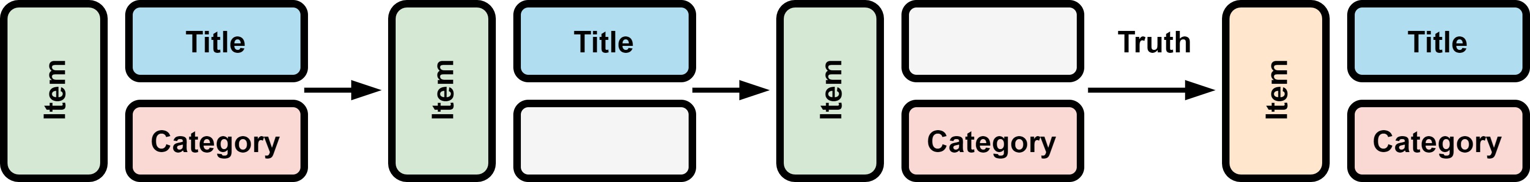
(a)

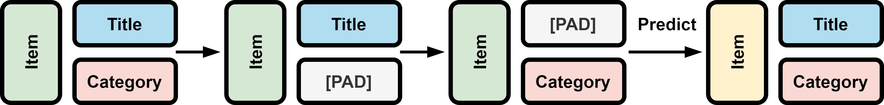
(b)

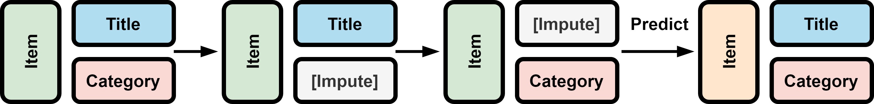
(c)

Figure 1. Sequential recommendation of items with side information. Gray blocks represent missing information. “[PAD]” (in (b)) indicates padding with generic or special values as often done in existing work. “[Impute]” (in (c)) indicates imputation with actual values for missing feature fields.

Some recent studies address the problem of missing side information in recommendation data. Wang et al. (2018) employ an auto-encoder (AE) with a modality dropout to recover the missing rating and side information. Shi et al. (2019) propose an adaptive feature sampling strategy to introduce more missing feature fields into the training process, which increases the robustness of the recommendation model against missing side information. Wu et al. (2020) define item recommendation and attribute inference in a user-item bipartite graph with attributes, and propose a graph convolutional network (GCN) (Kipf and Welling, 2017) based model to join these two tasks. However, the work just listed mainly targets non-sequential recommendation. Moreover, it treats item recommendation and side information imputation as different tasks.

In this work, we seek to design a sequential recommendation model that can handle missing feature fields of items in items sequences. The main challenge is how to adaptively impute missing information, including missing side information and the next item, according to the information available in the item sequence. First, we propose a task, the missing information imputation (MII) task that randomly masks some non-missing feature fields, including item IDs, in the input sequence, and then asks the model to recover them in the output. Since the next item to be recommended can also be seen as a missing feature field in the sequence, MII unifies the missing side information imputation task with the next item prediction task. MII can be considered as an extension of the masked item prediction task (Zeng et al., 2021) that only masks item IDs. Based on the MII task, we propose a sequential recommendation model, called missing information imputation recommender (MIIR), that jointly imputes missing side information and predicts the next item for the given item sequence. MIIR employs a dense fusion self-attention (DFSA) mechanism to fuse the information in IDs and other feature fields for predicting both missing side information and the next item. dense fusion self-attention (DFSA) captures the relation between any pair of feature fields in the input sequence, allowing it to fully fuse various types of (side) information to impute missing feature values and address the main recommendation challenge.

We conduct extensive experiments on three public datasets and show that MIIR significantly outperforms state-of-the-art sequential recommendation baselines. We also confirm that (i) imputing missing side information and (ii) DFSA both help to improve the performance of sequential recommendation.

The main contributions of this work are as follows:

• We propose to unify the missing side information imputation task and the sequential recommendation task through missing information imputation (MII). To the best of our knowledge, this is the first work of its kind in sequential recommendation.

• We present a novel sequential recommendation model, missing information imputation recommender (MIIR), that employs MII to provide the signal for simultaneously imputing the missing item side information and predicting the next item and dense fusion self-attention (DFSA) to fuse various information.

• We conduct extensive experiments on three public datasets to verify the effectiveness of MII, MIIR, and DFSA in sequential recommendation.

2. Related Work

In this section, we provide a review of research into sequential recommendation with side information, and research into missing side information in recommendation.

2.1. Sequential recommendation with side information

Side information fusion has been widely used in sequential recommendation because it can help to capture transition patterns among items. We classify existing work into work that uses self-attention and work that does not.

As to work that does not use self-attention, Hidasi et al. (2016b) employ parallel RNNs to extract the information from ID sequences of item IDs and sequences of features; they then examine different ways of combining the outputs of the RNNs. Zhou et al. (2020) propose self-supervised tasks to maximize the mutual information between an item and its attributes or between a sequence of item IDs and the sequence of their attributes. Yuan et al. (2021) construct a heterogeneous graph to aggregate different types of categorical attributes, then aggregate the representations of attribute types to get item representations.

Inspired by the success of self-attention mechanisms (Huang et al., 2018; Tang et al., 2018; Zhao et al., 2020), some work uses self-attention to fuse items and side information. Zhang et al. (2019) first use a vanilla attention mechanism to fuse different types of side information on each item, and then use two branches of self-attention blocks to model transition patterns between IDs and side information; they then concatenate the hidden states of the two blocks for item recommendation. Liu et al. (2021) propose a non-invasive self-attention mechanism that uses pure item ID representations as values and representations that integrate side information as queries and keys to calculate the attention. Xie et al. (2022) decouple the non-invasive self-attention of different types of side information to get fused attention matrices for items.

Although many methods have been proposed for sequential recommendation with side information, they (i) neglect the missing information problem, and use fixed special values to fill missing feature fields, which might harm the performance, and (ii) hardly explore the relation between an item and the side information of other items in the same sequence. These are aspects that we contribute on top of prior work.

2.2. Missing side information in recommendation

In real-world applications, the side information of users and items may be incomplete or missing, which may hurt the performance of recommendation models that rely on side information.

The traditional way to solve the problem of missing side information is to fill the missing feature fields with heuristic values (Lee et al., 2018; Biessmann et al., 2018; Shi et al., 2019), such as the most frequent feature values, average values, randomized values, the value unknown, or padding. As some studies have reported, these special values are independent of the context, and using them may lead to biased parameter estimation and prediction (Marlin and Zemel, 2009; Hernández-Lobato et al., 2014). Another way to deal with missing feature fields is to impute their missing values. Early approaches use KNN-based methods (Pan et al., 2015) or auto-encoders (AEs) (Beaulieu-Jones and Moore, 2017; Pereira et al., 2020) to predict the missing data. Wang et al. (2018) propose an AE-based model with modality dropout, which randomly drops representations of user or item information of different modalities in hidden states and reconstructs them by an AE. Cao et al. (2019) present a translation-based recommendation model that models preferences as translations from users to items, and jointly trains it with a knowledge graph (KG) completion model that predicts the missing relations in the KG for incorporating knowledge into the recommendation model. Instead of imputing the missing side information, Shi et al. (2019) propose an adaptive feature sampling strategy, which employs layer-wise relevance propagation (Binder et al., 2016) to calculate the importance of different features and samples features to make the model more robust against unknown features. Wu et al. (2020) propose a GCN-based model to jointly predict users’ preferences to items and predict the missing attribute values of users or items.

What we add on top of prior work on missing information in recommendation is that we focus on missing information in the context of sequential recommendation.

3. Method

3.1. Overview

Before going into details of the proposed MII task and MIIR model, we introduce notation used in this paper. We denote the item set as $I=\{\mathbf{i}_{1},\ldots,\mathbf{i}_{N_{i}}\}$, where $N_{i}$ is the number of items and each item ID $\mathbf{i}_{k}\in\mathbb{R}^{N_{i}}$ is represented as a one-hot vector. In addition to IDs, items have other feature fields corresponding to their side information. In this work, we consider categorical feature fields, including category and brand, and textual feature fields, including title and description. We denote the category set as $C=\{\mathbf{c}_{1},\ldots,\mathbf{c}_{N_{c}}\}$, where $N_{c}$ is the number of categories and each category $\mathbf{c}_{k}\in\mathbb{R}^{N_{c}}$ is a one-hot vector. Similarly, we denote the brand set as $B=\{\mathbf{b}_{1},\ldots,\mathbf{b}_{N_{b}}\}$, where $N_{b}$ is the number of brands and each brand $\mathbf{b}_{k}\in\mathbb{R}^{N_{b}}$. For titles and descriptions of items, we employ BERT (Devlin et al., 2019) to encode them into fixed-length vectors of size $768$. We denote all titles and all descriptions as $T=\{\mathbf{t}_{1},\ldots,\mathbf{t}_{N_{i}}\}$ and $D=\{\mathbf{d}_{1},\ldots,\mathbf{d}_{N_{i}}\}$, respectively, where $\mathbf{t}_{k}$ and $\mathbf{d}_{k}\in\mathbb{R}^{768}$. We use $S=[s_{1},\ldots,s_{n}]$ to denote a sequence with $n$ items, where $s_{k}=[\mathbf{s}^{i}_{k},\mathbf{s}^{c}_{k},\mathbf{s}^{b}_{k},\mathbf{s}^{t}_{k},\mathbf{s}^{d}_{k}]$ is the sequence of features fields of the $k$-th item, $\mathbf{s}^{i}_{k}\in I$, $\mathbf{s}^{c}_{k}\subseteq C$, $\mathbf{s}^{b}_{k}\in B$, $\mathbf{s}^{t}_{k}\in T$, and $\mathbf{s}^{d}_{k}\in D$. As an item may have multiple categories, we let $\mathbf{s}^{c}_{k}$ be a subset of $C$, which can be represented as a multi-hot vector $\mathbf{s}^{c}_{k}\in\mathbb{R}^{N_{c}}$. For missing item IDs, categories and brands, we have special one-hot vectors denoted as $\mathbf{i}_{miss}\in I$, $\mathbf{c}_{miss}\in C$ and $\mathbf{b}_{miss}\in B$, respectively. For missing titles and descriptions, we use the vector of “[CLS][SEP]” encoded by BERT to represent them, which are denoted as $\mathbf{t}_{miss}\in T$ and $\mathbf{d}_{miss}\in D$, respectively. These missing representations will be used in both MIIR and the baselines. It is worth noting that other feature fields can be formalized and modeled in a similar way.

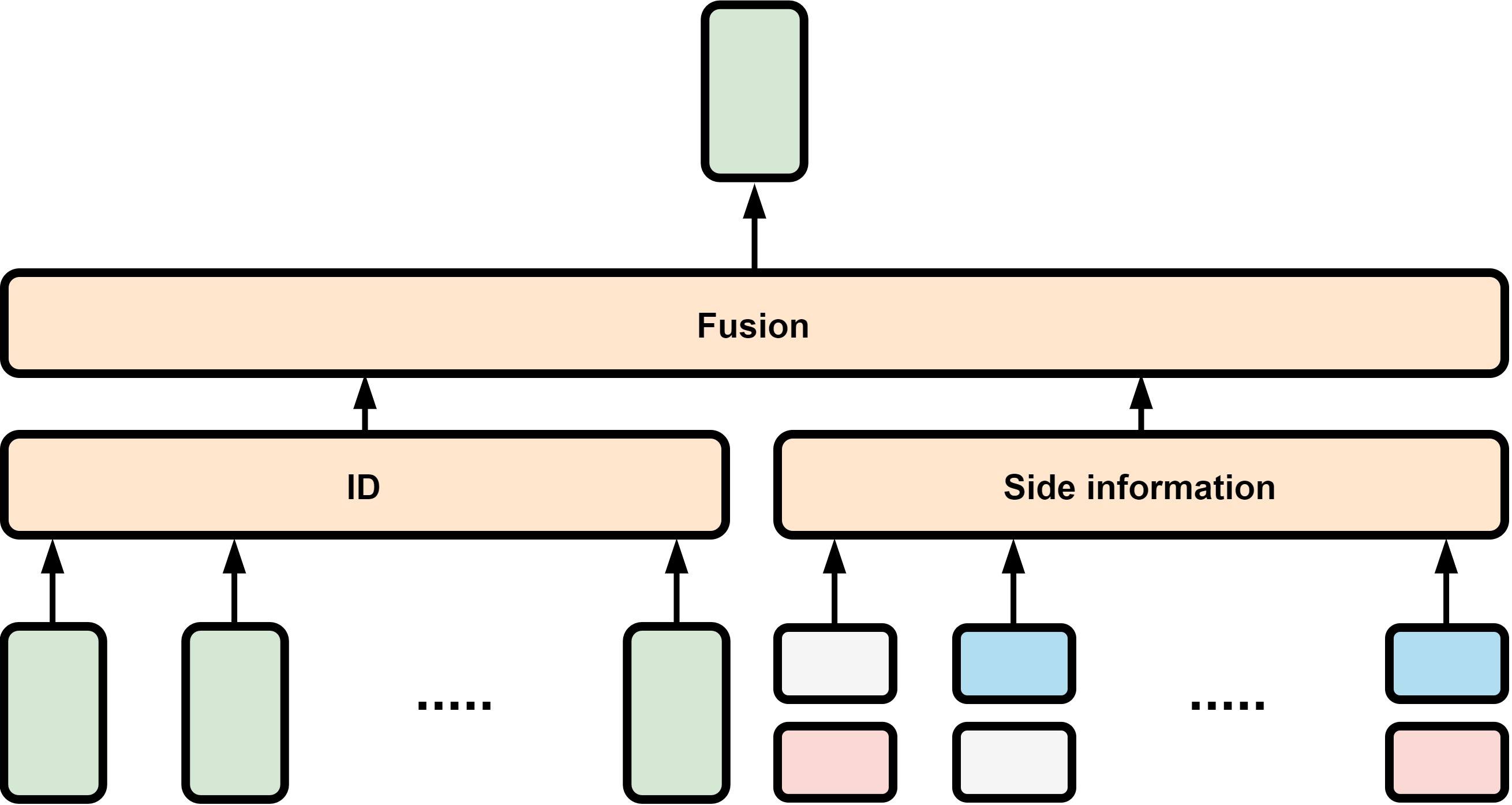
(a)

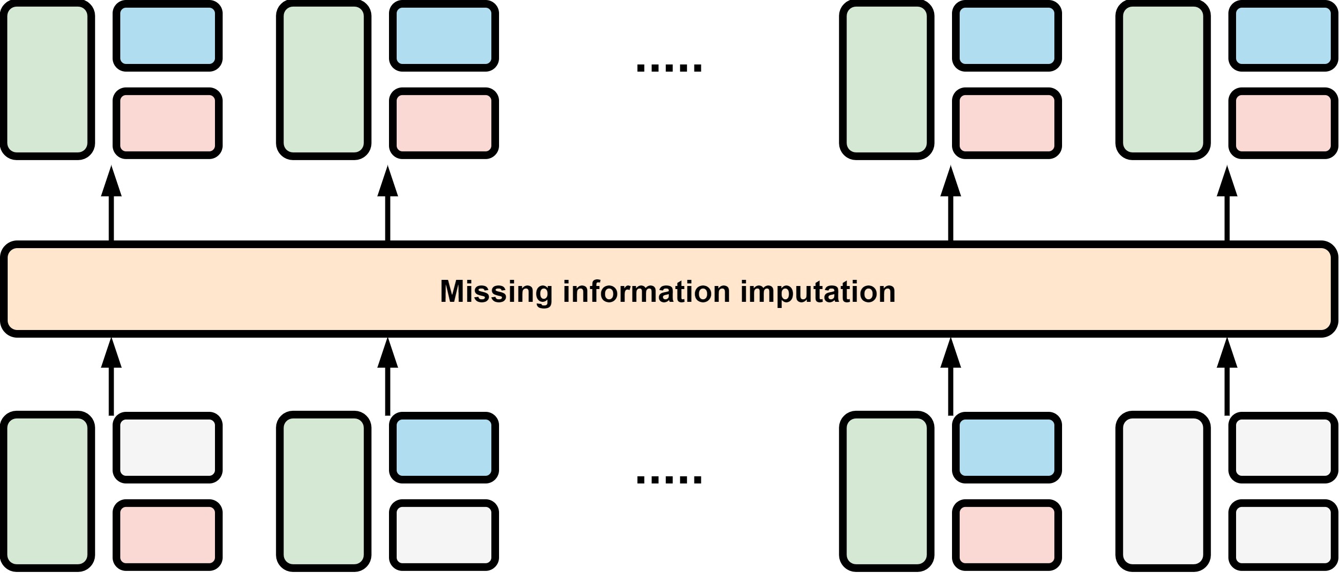
(b)

Figure 2. Comparing the sequential recommendation task and the missing information imputation task. (Same visual conventions as in Fig. 1.)

The missing information imputation task is to impute the values of the missing feature fields in $S$. The sequential recommendation task is to predict the next item $s_{n+1}$ for $S$. By appending a new item $s_{n+1}=[\mathbf{i}_{miss},\mathbf{c}_{miss},\mathbf{b}_{miss},\mathbf{t}_{miss},\mathbf{d}_{miss}]$ to the end of $S$ and imputing the $\mathbf{i}_{miss}$ of $s_{n+1}$, we can formulate the next item prediction task as a special case of missing information imputation task. In Fig. 2, we compare the sequential recommendation task and the missing information imputation task. In the sequential recommendation task, the next item is not considered as a missing data. In the missing information imputation task, the next item is simply a missing feature field. A model for the missing information imputation task that follows a unified way to impute both the next item and the other missing side information can be used for sequential recommendation.

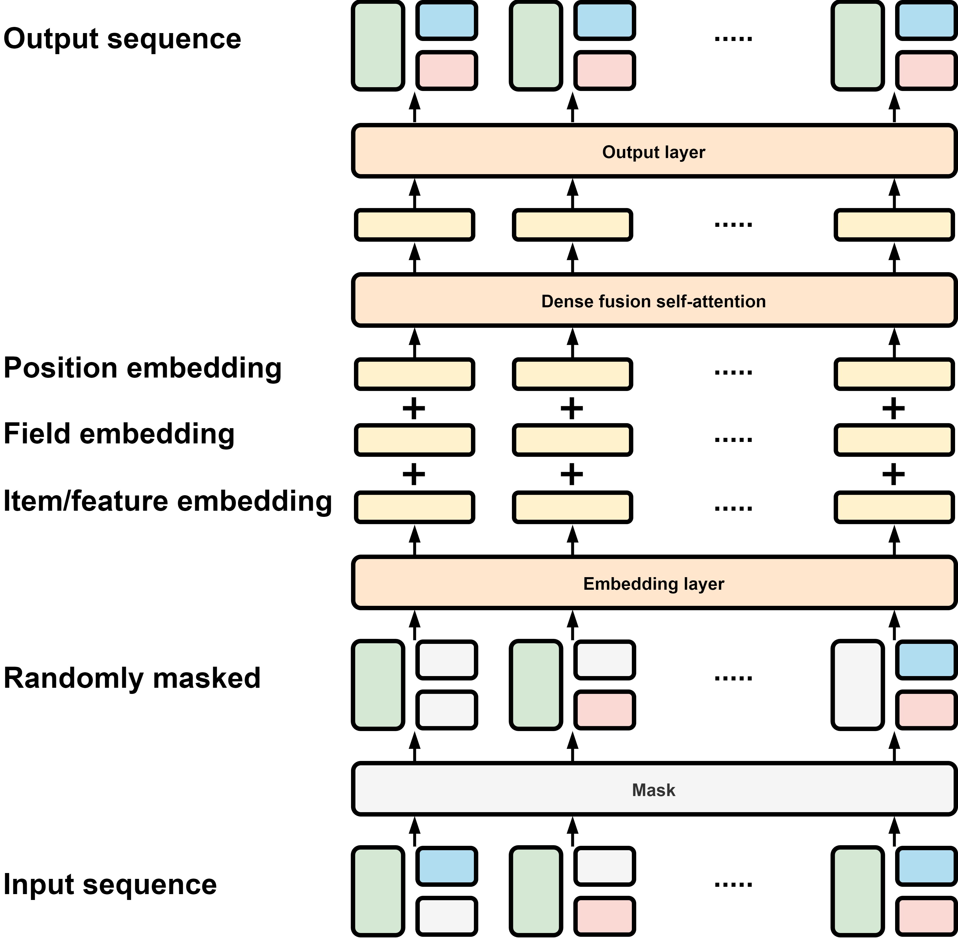
Figure 3. Architecture of the missing information imputation recommender (MIIR). MIIR takes a sequence of randomly masked feature fields as input. It transforms the input sequence into embeddings using the embedding layer. Then it employs a dense fusion self-attention mechanism to fuse information in the sequence. Finally, MIIR uses an output layer to reconstruct the input sequence and calculate the MII loss on masked feature fields. (Same visual conventions as in Fig. 1.)

To unify the missing side information imputation and next item recommendation tasks, we propose a sequential recommendation model called missing information imputation recommender (MIIR). As we illustrate in Fig. 3, MIIR consists of three main components: (i) an embedding layer, (ii) a dense fusion self-attention (DFSA) mechanisms, and (iii) an output layer. First, the embedding layer translates the input sequence into a series of embeddings. Then, the DFSA mechanism employs several transformer (Vaswani et al., 2017) layers to model the relation between any pair of feature fields in the sequence and fuse side information into the model for both imputation and recommendation. Finally, the output layer imputes the missing feature values including item IDs in the sequence based on the output of DFSA. Next, we will introduce the details of these main components.

3.2. Embedding layer

The embedding layer projects all item feature fields in the input sequence into low-dimensional dense vectors with a unified length.

For the $k$-th item $s_{k}=[\mathbf{s}^{i}_{k},\mathbf{s}^{c}_{k},\mathbf{s}^{b}_{k},\mathbf{s}^{t}_{k},\mathbf{s}^{d}_{k}]$ in the given sequence $S$, the embedding layer uses different ways to translate different feature fields. For the high-dimensional sparse vectors of $\mathbf{s}^{i}_{k}$, $\mathbf{s}^{c}_{k}$ and $\mathbf{s}^{b}_{k}$, we follow Eq. 1 to get the item embedding $\mathbf{e}^{i}_{k}\in\mathbb{R}^{e}$, the category embedding $\mathbf{e}^{c}_{k}\in\mathbb{R}^{e}$, and the brand embedding $\mathbf{e}^{b}_{k}\in\mathbb{R}^{e}$:

(1) $$\begin{split}\mathbf{e}^{i}_{k}&=\mathbf{E}^{i}\mathbf{s}^{i}_{k},\\ \mathbf{e}^{c}_{k}&=\mathbf{E}^{c}\mathbf{s}^{c}_{k},\\ \mathbf{e}^{b}_{k}&=\mathbf{E}^{b}\mathbf{s}^{b}_{k},\end{split}$$

where $\mathbf{E}^{i}\in\mathbb{R}^{e\times{N_{i}}}$ is the item embedding matrix, $\mathbf{E}^{c}\in\mathbb{R}^{e\times{N_{c}}}$ is the category embedding matrix, $\mathbf{E}^{b}\in\mathbb{R}^{e\times{N_{b}}}$ is the brand embedding matrix, and $e$ is the embedding size. For the high-dimensional dense vectors of $\mathbf{s}^{t}_{k}$ and $\mathbf{s}^{d}_{k}$, we project them into low-dimensional embeddings, i.e., the title embedding $\mathbf{e}^{t}_{k}\in\mathbb{R}^{e}$ and the description embedding $\mathbf{e}^{d}_{k}\in\mathbb{R}^{e}$, respectively, using Eq. 2:

(2) $$\begin{split}\mathbf{e}^{t}_{k}&=\mathbf{E}^{t}\mathbf{s}^{t}_{k},\\ \mathbf{e}^{d}_{k}&=\mathbf{E}^{d}\mathbf{s}^{d}_{k},\end{split}$$

where $\mathbf{E}^{t}\in\mathbb{R}^{e\times{768}}$ and $\mathbf{E}^{d}\in\mathbb{R}^{e\times{768}}$ are the projection matrices.

In order to distinguish different types of feature fields for the same item, we learn a field embedding for each type of feature fields. We denote the field embeddings of ID, category, brand, title and description as $\mathbf{f}^{i}$, $\mathbf{f}^{c}$, $\mathbf{f}^{b}$, $\mathbf{f}^{t}$ and $\mathbf{f}^{d}\in\mathbb{R}^{e}$, respectively. To distinguish the items in different positions of the same sequence, we also inject the position information into the model by learning position embeddings, where the $k$-th position embedding is denoted as $\mathbf{p}_{k}\in\mathbb{R}^{e}$. Finally, we add each field embedding to the corresponding item or feature embedding of $s_{k}$, and add $\mathbf{p}_{k}$ to all embeddings of $s_{k}$, as shown in Eq. 3:

(3) $$\mathbf{H}_{k}=\begin{bmatrix}\mathbf{h}^{i}_{k}\\ \mathbf{h}^{c}_{k}\\ \mathbf{h}^{b}_{k}\\ \mathbf{h}^{t}_{k}\\ \mathbf{h}^{d}_{k}\end{bmatrix}=\begin{bmatrix}\mathbf{e}^{i}_{k}+\mathbf{f}^{i}+\mathbf{p}_{k}\\ \mathbf{e}^{c}_{k}+\mathbf{f}^{c}+\mathbf{p}_{k}\\ \mathbf{e}^{b}_{k}+\mathbf{f}^{b}+\mathbf{p}_{k}\\ \mathbf{e}^{t}_{k}+\mathbf{f}^{t}+\mathbf{p}_{k}\\ \mathbf{e}^{d}_{k}+\mathbf{f}^{d}+\mathbf{p}_{k}\end{bmatrix},$$

where $\mathbf{h}^{i}_{k}$, $\mathbf{h}^{c}_{k}$, $\mathbf{h}^{b}_{k}$, $\mathbf{h}^{t}_{k}$, $\mathbf{h}^{d}_{k}\in\mathbb{R}^{e}$, and $\mathbf{H}_{k}\in\mathbb{R}^{5\times{e}}$ is the hidden state of $s_{k}$ that is the stack of all embeddings of its feature fields in order.

3.3. Dense fusion self-attention

The dense fusion self-attention (DFSA) mechanism follows a unified way to impute missing feature fields, both item IDs and side information. To exploit the information in a given context for imputation, we need to model the relations between different feature fields and fuse the representations of various feature fields. DFSA calculates the attention values between any pair of feature fields and fuses the information of other feature fields based on the attention value. By calculating the attention value, DFSA captures all possible (hence dense) pairwise relations between feature fields to facilitate missing information imputation.

Specifically, we first stack the hidden states of all items in $S$ in order by Eq. 4:

(4) $$\mathbf{H}=\begin{bmatrix}\mathbf{H}_{1}\\ \mathbf{H}_{2}\\ \vdots\\ \mathbf{H}_{n}\end{bmatrix},$$

where $\mathbf{H}\in\mathbb{R}^{5n\times{e}}$ is the hidden state matrix of $S$. Then, DFSA employs a transformer with $L$ layers to update $\mathbf{H}$.

Each transformer layer $\mathrm{Trm}(\cdot)$ is composed of two sub-layers: (i) multi-head self-attention $\operatorname{MH}(\cdot)$ and (ii) position-wise feed-forward $\operatorname{PFFN}(\cdot)$, as defined in Eq. 5:

(5) $$\begin{split}\mathbf{H}^{l+1}&=\mathrm{Trm}(\mathbf{H}^{l})=\mathrm{LN}(\mathbf{\widetilde{H}}^{l}+\mathrm{Dropout}(\mathrm{PFFN}(\mathbf{\widetilde{H}}^{l})))\\ \mathbf{\widetilde{H}}^{l}&=\mathrm{LN}(\mathbf{H}^{l}+\mathrm{Dropout}(\mathrm{MH}(\mathbf{H}^{l})))\\ \mathrm{MH}(\mathbf{H}^{l})&=[head_{1};\ldots;head_{h}]\mathbf{W}^{H}\\ head_{i}&=\mathrm{Attn}(\mathbf{H}^{l}\mathbf{W}^{Q}_{i},\mathbf{H}^{l}\mathbf{W}^{K}_{i},\mathbf{H}^{l}\mathbf{W}^{V}_{i})\\ \mathrm{Attn}(\mathbf{Q},\mathbf{K},\mathbf{V})&=\mathrm{softmax}(\mathbf{Q}\mathbf{K}^{\top}/\sqrt{e}+\mathbf{M})\mathbf{V}\\ \mathrm{PFFN}(\mathbf{\widetilde{H}}^{l})&=\mathrm{GELU}(\mathbf{\widetilde{H}}^{l}\mathbf{W}^{F}_{1}+\mathbf{b}^{F}_{1})\mathbf{W}^{F}_{2}+\mathbf{b}^{F}_{2},\end{split}$$

where $\mathrm{LN}$ is layer normalization (Ba et al., 2016), $\mathrm{Dropout}$ is dropout (Srivastava et al., 2014), $\mathrm{Attn}$ is attention, $\mathrm{GELU}$ is a Gaussian error linear unit activation (Hendrycks and Gimpel, 2016), $[\ldots;\ldots]$ is the concatenation operation, $h$ is the number of heads, $\mathbf{W}^{H}\in\mathbb{R}^{e\times{e}}$, $\mathbf{W}^{Q}_{i}$, $\mathbf{W}^{K}_{i}$, $\mathbf{W}^{V}_{i}\in\mathbb{R}^{e\times{e/h}}$, $\mathbf{W}^{F}_{1}\in\mathbb{R}^{e\times{4e}}$, $\mathbf{W}^{F}_{2}\in\mathbb{R}^{4e\times{e}}$, $\mathbf{b}^{F}_{1}\in\mathbb{R}^{4e}$ and $\mathbf{b}^{F}_{2}\in\mathbb{R}^{e}$ are trainable parameters, $\mathbf{H}^{l}$ and $\mathbf{H}^{l+1}\in\mathbb{R}^{5n\times{e}}$ are the output hidden state matrices in the $l$-th layer and the $(l+1)$-th layer, and $\mathbf{H}^{0}=\mathbf{H}$.

The matrix $\mathbf{M}\in\mathbb{R}^{5n\times{5n}}$ in Eq. 5 is the attention mask which is defined as:

(6) $$\mathbf{M}^{j,y}_{i,x}=\left\{\begin{array}[]{ll}0,&\textrm{allow to attend,}\\ -\infty,&\textrm{prevent from attending,}\end{array}\right.$$

where $i$ and $j\in\{1,\ldots,n\}$, $x$ and $y\in\{i,c,b,t,d\}$, $\mathbf{M}^{j,y}_{i,x}\in\mathbf{M}$ is the mask to control whether the feature field $\mathbf{s}^{y}_{j}$ can attend to the feature field $\mathbf{s}^{x}_{i}$. We set all $\mathbf{M}^{j,y}_{i,x}=0$, which means we allow to attend between any pair of feature fields in the sequence. Therefore, the DFSA can model relations and fuse information between all possible pairs of feature fields to facilitate both imputation and recommendation.

3.4. Output layer

The output layer reconstructs the input feature fields based on the output hidden states of DFSA. First, we split the final output hidden state matrix $\mathbf{H}^{L}$ of DFSA by Eq. 7:

(7) $$\mathbf{H}^{L}=\widehat{\mathbf{E}}=\begin{bmatrix}\widehat{\mathbf{E}}_{1}\\ \widehat{\mathbf{E}}_{2}\\ \vdots\\ \widehat{\mathbf{E}}_{n}\end{bmatrix},\quad\textrm{where }\widehat{\mathbf{E}}_{k}=\begin{bmatrix}\hat{\mathbf{e}}^{i}_{k}\\ \hat{\mathbf{e}}^{c}_{k}\\ \hat{\mathbf{e}}^{b}_{k}\\ \hat{\mathbf{e}}^{t}_{k}\\ \hat{\mathbf{e}}^{d}_{k}\end{bmatrix},$$

and $\hat{\mathbf{e}}^{i}_{k}$, $\hat{\mathbf{e}}^{c}_{k}$, $\hat{\mathbf{e}}^{b}_{k}$, $\hat{\mathbf{e}}^{t}_{k}$, $\hat{\mathbf{e}}^{d}_{k}\in\mathbb{R}^{e}$. Similar to the embedding layer, the output layer takes different ways to reconstruct different types of feature fields. Specifically, for the categorical feature fields, we calculate the probability distributions $\mathbf{p}^{i}_{k}\in\mathbb{R}^{N_{i}}$, $\mathbf{p}^{c}_{k}\in\mathbb{R}^{N_{c}}$ and $\mathbf{p}^{b}_{k}\in\mathbb{R}^{N_{b}}$ of the item ID, category and brand of the $k$-th item $s_{k}$ as follows:

(8) $$\begin{split}\mathbf{p}^{i}_{k}&=\mathrm{softmax}({\mathbf{E}^{i}}^{\top}\hat{\mathbf{e}}^{i}_{k})\\ \mathbf{p}^{c}_{k}&=\mathrm{sigmoid}({\mathbf{E}^{c}}^{\top}\hat{\mathbf{e}}^{c}_{k})\\ \mathbf{p}^{b}_{k}&=\mathrm{softmax}({\mathbf{E}^{b}}^{\top}\hat{\mathbf{e}}^{b}_{k}),\end{split}$$

where $\mathbf{E}^{i}\in\mathbb{R}^{e\times{N_{i}}}$, $\mathbf{E}^{c}\in\mathbb{R}^{e\times{N_{c}}}$, $\mathbf{E}^{b}\in\mathbb{R}^{e\times{N_{b}}}$ are the re-used item embedding matrix, category embedding matrix, and brand embedding matrix in the embedding layer, respectively. Note that we regard each category prediction as binary classification, because an item may contain multiple categories. Then we obtain the reconstructed item ID $\hat{\mathbf{s}}^{i}_{k}\in\mathbb{R}^{N_{i}}$, category $\hat{\mathbf{s}}^{c}_{k}\in\mathbb{R}^{N_{c}}$ and brand $\hat{\mathbf{s}}^{b}_{k}\in\mathbb{R}^{N_{b}}$ based on the probability distributions, as shown in Eq. 9:

(9) $$\begin{split}\hat{\mathbf{s}}^{i}_{k}&=\mathrm{argmax}(\mathbf{p}^{i}_{k})\\ \hat{\mathbf{s}}^{c}_{k}&=\mathbf{1}(\mathbf{p}^{c}_{k}>0.5)\\ \hat{\mathbf{s}}^{b}_{k}&=\mathrm{argmax}(\mathbf{p}^{b}_{k}),\end{split}$$

where $\mathbf{1}(\alpha)$ is the indicator function that equals 1 if $\alpha$ is true and 0 otherwise. Meanwhile, for the textual feature fields, we follow Eq. 10 to get the reconstructed title $\hat{\mathbf{s}}^{t}_{k}\in\mathbb{R}^{768}$ and description $\hat{\mathbf{s}}^{d}_{k}\in\mathbb{R}^{768}$ directly:

(10) $$\begin{split}\hat{\mathbf{s}}^{t}_{k}&=\mathbf{O}^{t}\hat{\mathbf{e}}^{t}_{k},\\ \hat{\mathbf{s}}^{d}_{k}&=\mathbf{O}^{d}\hat{\mathbf{e}}^{d}_{k},\end{split}$$

where $\mathbf{O}^{t}\in\mathbb{R}^{768\times{e}}$ and $\mathbf{O}^{d}\in\mathbb{R}^{768\times{e}}$ are the projection matrices.

3.5. Missing information imputation loss

We train MIIR with MII. MII first randomly masks feature fields in the sequence with probability $p$, i.e., replacing a non-missing feature value with the corresponding missing feature value $\mathbf{i}_{miss}$, $\mathbf{c}_{miss}$, $\mathbf{b}_{miss}$, $\mathbf{t}_{miss}$ or $\mathbf{d}_{miss}$. For the $k$-th item $s_{k}$ in the sequence $S$, we use $m^{i}_{k}$, $m^{c}_{k}$, $m^{b}_{k}$, $m^{t}_{k}$ and $m^{d}_{k}\in\{\mathit{true},\mathit{false}\}$ to denote whether its ID, category, brand, title and description are masked. Then, MIIR learns to recover the masked feature fields by MII and impute the missing feature values based on the context.

Specifically, there are differences in the calculation of the missing information imputation loss for different types of feature fields. For the categorical feature fields (i.e., ID, category and brand), our goal is to minimize the cross-entropy loss:

(11) $$\begin{split}L^{i}_{k}&=-\mathbf{1}(m^{i}_{k}){\mathbf{s}^{i}_{k}}^{\top}\log(\mathbf{p}^{i}_{k})\\ L^{c}_{k}&=-\mathbf{1}(m^{c}_{k})({\mathbf{s}^{c}_{k}}^{\top}\log(\mathbf{p}^{c}_{k})+(1-{\mathbf{s}^{c}_{k}}^{\top})\log(1-\mathbf{p}^{c}_{k}))/N_{c}\\ L^{b}_{k}&=-\mathbf{1}(m^{b}_{k}){\mathbf{s}^{b}_{k}}^{\top}\log(\mathbf{p}^{b}_{k}),\end{split}$$

where $L^{i}_{k}$, $L^{c}_{k}$ and $L^{b}_{k}$ are the imputation loss for the item ID, category and brand of $s_{k}$, respectively. For the textual feature fields (i.e., title and description), our goal is to minimize the mean square error loss:

(12) $$\begin{split}L^{t}_{k}&=\mathbf{1}(m^{t}_{k})\|\mathbf{s}^{t}_{k}-\hat{\mathbf{s}}^{t}_{k}\|^{2}\\ L^{d}_{k}&=\mathbf{1}(m^{d}_{k})\|\mathbf{s}^{d}_{k}-\hat{\mathbf{s}}^{d}_{k}\|^{2},\end{split}$$

where $L^{t}_{k}$ and $L^{d}_{k}$ are the imputation loss for the title and description of $s_{k}$. The missing information imputation objective of the entire model on $S$ is shown in Eq. 13:

(13) $$\begin{split}L^{mii}_{S}&=1/n\sum^{n}_{k=1}L^{\mathit{mii}}_{k}\\ L^{mii}_{k}&=L^{i}_{k}+L^{c}_{k}+L^{b}_{k}+L^{t}_{k}+L^{d}_{k}.\end{split}$$

Note that since the item ID is one of the feature fields and the next item prediction is a MII task, MIIR trained by MII can directly be applied to sequential recommendation.

In our experiments, we also consider further fine-tuning MIIR or directly training MIIR with the masked item prediction loss to make the model only focus on the item prediction task. Specifically, we randomly mask all feature fields of some items in the given sequence, while let MIIR predict the masked item IDs only. The recommendation loss (i.e., the masked item prediction loss) on $S$ is defined as:

(14) $$\begin{split}L^{\mathit{rec}}_{S}&=1/n\sum^{n}_{k=1}L^{\mathit{rec}}_{k}\\ L^{\mathit{rec}}_{k}&=L^{i}_{k}=-\mathbf{1}(m^{i}_{k}){\mathbf{s}^{i}_{k}}^{\top}\mathrm{log}(\mathbf{p}^{i}_{k}),\end{split}$$

where $L^{\mathit{rec}}_{k}$ is the recommendation loss for $s_{k}$.

4. Experimental Setup

4.1. Research questions

In this paper, we seek to answer the following research questions:

1. How does MIIR perform on the sequential recommendation task compared to state-of-the-art methods?

2. What are the benefits of training MIIR with MII?

3. Does modeling the relation between any pair of feature fields in item sequences help sequential recommendation?

4. What is the performance of MIIR on imputing missing side information?

4.2. Datasets

There are many public datasets for experimenting with sequential recommendation; see (Fang et al., 2020). However, we need sequential recommendation datasets that come with side information. We conduct experiments on three public datasets: “Beauty”, “Sports and Outdoors” and “Toys and Games” (Ni et al., 2019), as they have rich item side information, including category, brand, title and description.

We follow common practices (Zhang et al., 2019; Liu et al., 2021) to process the datasets. We sort each user’s records in chronological order to construct an item sequence. We filter out item sequences whose length is less than $5$ to avoid noise from the cold-start problem. For each item sequence, we use the last item for test, the second last item for validation, and the rest items for training. For each test or validation item, we randomly sample $99$ negative items for ranking. We randomly discard side information of items with probability $0.5$. We use “Beauty D”, “Sports and Outdoors D” and “Toys and Games D” to denote the datasets after discarding side information. The statistics of the datasets after pre-processing are summarized in Table 1.

Table 1. Summary of the datasets. The missing rate is the percentage of missing feature fields in all feature fields. Especially, “Missing rate D” is the missing rate after discarding side information.

Dataset	Beauty	Sports and Outdoors	Toys and Games
#items	121,291	194,715	164,978
#sequences	52,374	84,368	58,314
Average length	8.97	8.50	8.99
#categories	656	3,035	957
#brands	13,188	14,163	14,135
Missing rate	12.54%	20.11%	11.20%
Missing rate D	56.32%	60.12%	55.51%

4.3. Baselines

We compare MIIR with the following recommendation baselines, which can be grouped into (i) methods without side information fusion, (ii) methods with side information fusion, and (iii) methods with missing feature values.

• Methods without side information fusion:

  • GRU4Rec employs RNNs to capture sequential patterns between items for sequential recommendation (Hidasi et al., 2016a).

  • SASRec uses the self-attention mechanism to model item sequences for next item recommendations (Kang and McAuley, 2018).

  • BERT4Rec uses a bidirectional self-attention network train-ed by a masked item prediction task for sequential recommendation (Sun et al., 2019).

• Methods with side information fusion:

  • PRNN employs parallel RNNs to process items and their side information respectively, then combines the hidden states of the RNNs for next item prediction (Hidasi et al., 2016b).

  • FDSA leverages two separate self-attention networks to model the ID transition patterns and the feature transition patterns respectively, then concatenates the outputs of two networks for next item prediction (Zhang et al., 2019).

  • NOVA adopts a non-invasive self-attention mechanism to leverage side information under the BERT4Rec framework for sequential recommendation (Liu et al., 2021).

• Methods with missing feature values:

  • RFS randomly samples feature fields to introduce more missing information during training (Shi et al., 2019). RFS aims to make the model more robust with missing feature values instead of imputing missing feature fields. We combine RFS with FDSA and NOVA, and denote the variants as FDSA+RFS and NOVA+RFS.

  • LRMM designs an auto-encoder with modality dropout to impute both user ratings and missing side information for each item (Wang et al., 2018). LRMM is not proposed for sequential recommendation. Therefore, we use the imputed missing side information by LRMM to train FDSA and NOVA, and denote them as FDSA+LRMM and NOVA+LRMM.

Other methods with side information fusion, such as (Zhou et al., 2020; Yuan et al., 2021), can only model categorical item side information; for a fair comparison, we do not consider them as baselines. In addition to the baselines listed above, we compare MIIR against four variants, namely MIIR-F, MIIR-R, MIIR-M, and Sparse-MIIR, to be defined in Section 5.1,  5.2 and  5.3.

We unify the sequential recommendation loss in all baselines, MIIR, and its variants to the cross-entropy loss, rather than the pairwise loss (Rendle et al., 2009), to avoid noise due to negative sampling in the pairwise loss.

4.4. Metrics and implementation

To evaluate the performance of sequential recommendation methods, we employ two widely used evaluation metrics: HR@$k$ (hit ratio) and MRR (mean reciprocal rank) (Fang et al., 2020), where $k\in\{5,10\}$.

• HR measures the proportion of the sequences whose ground-truth items are amongst the top ranked items in all test sequences.

• MRR is the average of reciprocal ranks of the ground-truth items.

For all baselines and our proposed model, we initialize the trainable parameters randomly with the Xavier method (Glorot and Bengio, 2010). We train all methods with the Adam optimizer (Kingma and Ba, 2015) for $100$ epochs, with a batch size of $128$ and a learning rate of $0.0001$. We also apply gradient clipping (Pascanu et al., 2013) with range $[-5,5]$ during training. According to the average length in Table 1, we set the maximum sequence length to $20$ for three datasets for all methods.

All hyper-parameters of the baselines are set following the suggestions from the original papers. For the hyper-parameters of MIIR, we set the embedding size $e$ to $64$, the number of heads $h$ to $4$, and the number of layers $L$ to $3$. We set the dropout rate in DFSA and the mask probability $p$ in MII to $0.5$.

To facilitate reproducibility of the results reported in this paper, the code and data used in experiments are available at https://github.com/TempSDU/MIIR.

5. Experimental Results

5.1. Overall performance

Table 2. Performance comparison of MIIR, variants, and the baselines on the “Beauty” dataset. MIIR-F is a variant of MIIR that is fine-tuned using the recommendation loss (see Section 5.1) and MIIR-R is a variant trained using the recommendation loss only (see Section 5.2). The highest overall performance is denoted in bold face. The highest performance among the baselines is underlined. Impr. (%) is the performance gain of MIIR against the best baseline method. $*$ indicates that an improvement is statistically significant based on a two-sided paired t-test with $p<0.05$.

	Beauty			Beauty D
Method	HR@5	HR@10	MRR	HR@5	HR@10	MRR
GRU4Rec	31.58	42.50	21.47	31.58	42.50	21.47
SASRec	32.83	43.61	23.16	32.83	43.61	23.16
BERT4Rec	33.22	43.77	23.58	33.22	43.77	23.58
PRNN	32.27	42.70	23.08	31.80	42.55	22.23
FDSA	35.22	44.83	25.39	35.02	44.68	25.33
NOVA	34.99	45.07	25.02	34.21	44.38	24.80
FDSA+RFS	35.45	45.40	25.68	34.73	44.56	25.17
NOVA+RFS	35.57	45.61	25.74	34.26	44.24	24.97
LRMM	22.74	32.95	17.09	18.04	26.94	13.96
FDSA+LRMM	35.35	45.15	25.62	35.10	44.73	25.52
NOVA+LRMM	35.35	45.31	25.50	34.31	44.53	25.01
MIIR	38.92	48.61	29.46	37.30	46.85	27.90
MIIR-F	38.73	48.01	29.28	37.12	46.48	27.95
MIIR-R	35.59	45.60	25.85	34.92	44.96	25.41
Impr. (%)	+3.35∗	+3.00∗	+3.72∗	+2.20∗	+2.12∗	+2.38∗

Table 3. Performance comparison of MIIR, variants, and the baselines on the “Sports and Outdoors” dataset.

	Sports and Outdoors			Sports and Outdoors D
Method	HR@5	HR@10	MRR	HR@5	HR@10	MRR
GRU4Rec	33.54	44.57	23.70	33.54	44.57	23.70
SASRec	34.46	44.69	25.41	34.46	44.69	25.41
BERT4Rec	35.12	45.24	26.11	35.12	45.24	26.11
PRNN	37.41	47.25	27.23	36.01	46.18	26.12
FDSA	39.16	48.08	29.27	37.30	46.74	27.20
NOVA	37.95	47.54	28.08	36.15	45.96	26.90
FDSA+RFS	38.18	47.18	28.31	37.17	46.65	27.01
NOVA+RFS	37.63	47.41	27.33	35.86	45.52	26.84
LRMM	28.65	41.36	20.50	19.79	30.34	15.13
FDSA+LRMM	39.48	48.52	29.41	38.46	47.67	28.24
NOVA+LRMM	38.18	47.76	28.30	37.28	46.78	27.32
MIIR	43.66	52.63	32.66	40.55	49.80	30.04
MIIR-F	42.66	51.49	32.01	39.98	48.98	29.86
MIIR-R	40.01	49.70	29.40	38.07	47.82	27.77
Impr. (%)	+4.18∗	+4.11∗	+3.25∗	+2.09∗	+2.13∗	+1.80∗

Table 4. Performance comparison of MIIR, variants, and the baselines on the “Toys and Games” dataset.

	Toys and Games			Toys and Games D
Method	HR@5	HR@10	MRR	HR@5	HR@10	MRR
GRU4Rec	31.19	42.15	21.90	31.19	42.15	21.90
SASRec	31.74	41.22	24.51	31.74	41.22	24.51
BERT4Rec	31.45	41.22	23.25	31.45	41.22	23.25
PRNN	34.00	44.25	24.32	32.71	42.98	23.23
FDSA	34.44	43.89	26.03	32.70	42.33	24.69
NOVA	34.50	44.34	25.86	34.00	43.74	25.06
FDSA+RFS	34.81	44.62	26.30	33.41	43.64	25.22
NOVA+RFS	35.33	45.29	26.27	33.39	43.26	24.73
LRMM	29.88	40.96	21.87	19.85	29.83	15.15
FDSA+LRMM	35.20	44.50	26.49	33.43	42.94	25.18
NOVA+LRMM	35.65	45.50	26.61	34.51	44.47	25.51
MIIR	40.11	49.80	29.64	39.01	48.89	28.74
MIIR-F	39.00	47.76	29.57	38.25	47.45	28.75
MIIR-R	35.80	45.37	26.00	34.69	44.30	24.81
Impr. (%)	+4.46∗	+4.30∗	+3.03∗	+4.50∗	+4.42∗	+3.23∗

To answer RQ1, we compare MIIR against the recommendation models listed in Section 4.3 on the three datasets from Section 4.2. Table 2, 3 and 4 list the evaluation results of all methods on each dataset, respectively. Based on these results, we have the following observations.

First, on all datasets, MIIR performs significantly better than all baselines by a large margin despite the different missing rates, in terms of HR@5, HR@10 and MRR. MIIR has two major advantages: (i) MIIRtrains the model using MII to enhance its ability to deal with missing side information in sequential recommendation (see detailed analysis in Section 5.2), and (ii) MIIRemploys DFSA to improve the side information fusion in the model (see Section 5.3 for further analysis).

Second, the item side information can help sequential recommender systems to more accurately model the transition patterns among items. To verify this, we divide all methods into three groups: (i) GRU4Rec and PRNN that are based on RNNs; (ii) SASRec and FDSA that are based on left-to-right self-attention networks; and (iii) BERT4Rec, NOVA, and MIIR that employ bidirectional self-attention networks and the masked item prediction task. In each group, we see that methods that fuse side information outperform methods that only rely on item IDs, which illustrates that item side information does help.

Third, the performance of PRNN, FDSA, NOVA and MIIR on the “Beauty”, “Sports and Outdoors” and “Toys and Games” datasets is higher than that on the discarded versions of the datasets (i.e., “Beauty D”, “Sports and Outdoors D” and “Toys and Games D”). We see two reasons for this difference: (i) the “Beauty D”, “Sports and Outdoors D” and “Toys and Games D” datasets discard some side information, so the available side information becomes less, and (ii) using the special values (i.e., $\mathbf{i}_{miss}$, $\mathbf{c}_{miss}$, $\mathbf{b}_{miss}$, $\mathbf{t}_{miss}$ and $\mathbf{d}_{miss}$) to fill missing feature fields may be harmful to PRNN, FDSA and NOVA.

Fourth, by comparing FDSA+RFS and NOVA+RFS with FDSA and NOVA, we can see that RFS does not consistently improve the performance of FDSA and NOVA on all datasets. RFS even degrades the performance of FDSA and NOVA in some cases. Because RFS introduces more missing feature values into the model training instead of imputing missing feature fields, it does not deal with the missing side information problem fundamentally.

Fifth, the performance of LRMM is significantly worse than that of the sequential recommendation models with side information. LRMM even performs worse than GRU4Rec, SASRec and BERT4Rec that neglect the item side information. The main reason is that LRMM is not a sequential model, so it does not exploit the relation and information in sequences to make recommendation and imputation, both of which are essential in the sequential recommendation task. We can also observe that FDSA+LRMM and NOVA+LRMM outperform FDSA and NOVA, which verifies the effectiveness of the imputation results of LRMM. This also demonstrates that imputing missing feature values is a better way to alleviate the missing side information problem than using fixed special values and RFS.

Sixth, modeling sequential recommendation as missing information imputation is sufficient to train a recommendation model. To verify this, we conduct an experiment that first pre-trains MIIR using the missing information imputation loss (Eq. 13), and then fine-tunes it using the recommendation loss (Eq. 14). We use MIIR-F to denote this variant of MIIR. In Table 2 we see that MIIR-F performs worse than MIIR in most cases. Fine-tuning MIIR-F with the recommendation loss might lead to overfitting, resulting in performance decreases. This result supports the conclusion that with MII we can unify the sequential recommendation task as a particular type of missing information imputation task to train MIIR together with the other imputation task for missing item side information.

5.2. Benefits of MII

Table 5. Performance comparison to assess the use of missing feature fields on the “Beauty” dataset. MIIR-M and MIIR-R-M are the variants of MIIR and MIIR-R respectively that mask missing feature fields in self-attention (see Section 5.2).

	Beauty			Beauty D
Method	HR@5	HR@10	MRR	HR@5	HR@10	MRR
MIIR	38.92	48.61	29.46	37.30	46.85	27.90
MIIR-R	35.59	45.60	25.85	34.92	44.96	25.41
MIIR-M	39.16	48.67	29.45	37.12	46.58	27.83
MIIR-R-M	36.40	46.31	27.11	34.71	45.01	25.42

Table 6. Performance comparison to assess the use of missing feature fields on the “Sports and Outdoors” dataset.

	Sports and Outdoors			Sports and Outdoors D
Method	HR@5	HR@10	MRR	HR@5	HR@10	MRR
MIIR	43.66	52.63	32.66	40.55	49.80	30.04
MIIR-R	40.01	49.70	29.40	38.07	47.82	27.77
MIIR-M	43.04	52.12	32.16	40.36	49.65	29.81
MIIR-R-M	39.71	48.98	29.15	38.33	48.10	28.12

Table 7. Performance comparison to assess the use of missing feature fields on the “Toys and Games” dataset.

	Toys and Games			Toys and Games D
Method	HR@5	HR@10	MRR	HR@5	HR@10	MRR
MIIR	40.11	49.80	29.64	39.01	48.89	28.74
MIIR-R	35.80	45.37	26.00	34.69	44.30	24.81
MIIR-M	39.33	49.22	28.97	37.80	47.58	27.82
MIIR-R-M	35.22	45.29	26.28	34.53	44.47	25.58

To answer RQ2, we analyze how MIIR benefits from training with MII.

In Table 2, 3 and 4, we report on results of a variant of MIIR that directly trains MIIR with the recommendation loss shown in Eq. 14. We write MIIR-R for this variant of MIIR without the supervised signal of MII. When we compare the performance of MIIR and MIIR-R, we see very substantial gaps. This confirms the effectiveness of training MIIR with MII, which accounts for the main part of the improvement of MIIR over other methods.

To demonstrate that MIIR can mine useful information from missing feature fields by training with MII, we design a variant of MIIR called MIIR-M by masking missing feature fields. In MIIR-M, we revise the attention mask $\mathbf{M}$ used in Eq. 5, which is a null matrix in MIIR. The revision in $\mathbf{M}$ is defined as:

(15) $$\mathbf{M}^{j,y}_{i,x}=\left\{\begin{array}[]{ll}-\infty,&\textrm{if $\mathbf{s}^{x}_{i}$ or $\mathbf{s}^{y}_{j}\in\{\mathbf{c}_{miss},\mathbf{b}_{miss},\mathbf{t}_{miss},\mathbf{d}_{miss}\}$,}\\ 0,&\textrm{otherwise,}\end{array}\right.$$

where the condition of $\mathbf{s}^{x}_{i}$ or $\mathbf{s}^{y}_{j}\in\{\mathbf{c}_{miss}$, $\mathbf{b}_{miss}$, $\mathbf{t}_{miss}$, $\mathbf{d}_{miss}\}$ depends on the original input sequence instead of the sequence after randomly masking. The purpose of the variant is to prevent the model from attending to the missing feature fields about item side information in the sequence. On the one hand, MIIR-M cannot mine and fuse any information in missing feature fields for sequential recommendation. On the other hand, MIIR-M is unable to exploit the information in non-missing feature fields to impute the missing side information. Besides, we mask missing feature fields for MIIR-R to analyze how missing feature values affect the performance of MIIR without MII, denoted as MIIR-R-M.

In Table 5, 6 and 7, we compare MIIR and MIIR-R with MIIR-M and MIIR-R-M, respectively. We find that MIIR outperforms MIIR-M in most cases, which indicates that MIIR is able to extract useful information from missing feature fields to improve the sequential recommendation performance. We also observe that MIIR-R-M performs better than MIIR-R in some cases. This phenomenon indicates that using fixed special values for filling missing feature fields hurts the model performance. Instead, masking missing feature fields is a better way without imputation. On the “Beauty” dataset, MIIR only achieves comparable performance with MIIR-M, and MIIR-R also performs worse than MIIR-R-M. However, the performance gap between MIIR and MIIR-M is smaller than that between MIIR-R and MIIR-R-M, and we have similar observations on other datasets. This illustrates that imputing missing feature values is to be preferred over masking them for alleviating the missing side information problem.

MIIR-M also outperforms all baselines on the three datasets with different missing rates. Training MIIR with MII helps MIIR to make use non-missing feature fields. Imputing the masked non-missing feature values requires the model to capture the relations between different feature fields, so MII guides MIIR to better fuse side information into the model for improving the sequential recommendation performance.

5.3. Effectiveness of DFSA

Table 8. Performance comparison of dense and sparse attention on the “Beauty” dataset. Sparse-MIIR and Sparse-MIIR-R are variants of MIIR and MIIR-R, respectively, in which DFSA is replaced by SFSA (see Section 5.3).

	Beauty			Beauty D
Method	HR@5	HR@10	MRR	HR@5	HR@10	MRR
MIIR	38.92	48.61	29.46	37.30	46.85	27.90
MIIR-R	35.59	45.60	25.85	34.92	44.96	25.41
Sparse-MIIR	36.71	46.60	26.87	36.04	45.98	26.34
Sparse-MIIR-R	34.95	45.02	25.35	34.61	44.84	25.19

Table 9. Performance comparison of dense and sparse attention on the “Sports and Outdoors” dataset.

	Sports and Outdoors			Sports and Outdoors D
Method	HR@5	HR@10	MRR	HR@5	HR@10	MRR
MIIR	43.66	52.63	32.66	40.55	49.80	30.04
MIIR-R	40.01	49.70	29.40	38.07	47.82	27.77
Sparse-MIIR	40.52	50.04	29.64	39.24	48.91	28.67
Sparse-MIIR-R	38.61	48.29	28.25	37.56	47.72	27.21

Table 10. Performance comparison of dense and sparse attention on the “Toys and Games” dataset.

	Toys and Games			Toys and Games D
Method	HR@5	HR@10	MRR	HR@5	HR@10	MRR
MIIR	40.11	49.80	29.64	39.01	48.89	28.74
MIIR-R	35.80	45.37	26.00	34.69	44.30	24.81
Sparse-MIIR	37.61	47.77	27.23	37.06	47.27	26.79
Sparse-MIIR-R	35.58	45.66	25.80	34.46	44.54	24.53

Table 11. Performance comparison of LRMM and MIIR for missing side information imputation on the “Beauty D”, “Sports and Outdoors D” and “Toys and Games D” datasets.

Dataset	Field	Metric	LRMM	MIIR
Beauty D	Category	Precision	70.1500	79.6400
		Recall	48.4100	36.9700
		F1	52.9600	48.6100
	Brand	Accuracy	07.8400	05.0100
	Title	Mean squared error	00.0871	00.0514
	Description	Mean squared error	00.1454	00.0704
Sports and Outdoors D	Category	Precision	57.0200	74.9700
		Recall	51.3100	35.9100
		F1	46.3800	46.4000
	Brand	Accuracy	06.0600	04.4300
	Title	Mean squared error	00.0927	00.0534
	Description	Mean squared error	00.1474	00.0835
Toys and Games D	Category	Precision	72.3200	89.3100
		Recall	51.0800	42.3100
		F1	54.1100	55.5000
	Brand	Accuracy	18.6100	14.4900
	Title	Mean squared error	00.0858	00.0514
	Description	Mean squared error	00.1427	00.0777

To answer RQ3, we conduct an ablation study to analyze the effectiveness of DFSA in MIIR.

We first compare MIIR-R, the variant of MIIR that is trained with recommendation loss only, with the baselines in Table 2, 3, 4. MIIR-R achieves better or comparable performance with the baselines on most evaluation metrics of all datasets, even without the help of MII. The main reason is that MIIR-R has dense fusion self-attention (DFSA) to better fuse information in the item sequence for improving sequential recommendation.

In order to validate that it is important to model all possible pairwise relations in an item sequence for sequential recommendation, we design another self-attention mechanism called sparse fusion self-attention (SFSA). sparse fusion self-attention (SFSA) modifies the attention mask $\mathbf{M}$ in Eq. 5 into:

(16) $$\mathbf{M}^{j,y}_{i,x}=\left\{\begin{array}[]{ll}0,&\textrm{if $i==j$ or $x==y$,}\\ -\infty,&\textrm{otherwise,}\end{array}\right.$$

where the condition $i==j$ or $x==y$ means that SFSA only allows to attend between the pair of feature fields belonging to the same item or the same type. Therefore, SFSA only models the relation between different feature fields of the same item or the relation between the same type of feature fields of different items in the sequence. These relations are also modeled in some baselines, such as PRNN and FDSA.

In Table 8, 9 and 10, we compare the performance of DFSA and SFSA as components of MIIR and MIIR-R. We write Sparse-MIIR and Sparse-MIIR-R for the variants of MIIR and MIIR-R, respectively, in which DFSA is replaced by SFSA. We can see that MIIR outperforms Sparse-MIIR on all datasets despite different missing rates. What’s more, MIIR-R outperforms Sparse-MIIR-R in most cases too. Modeling the relations between any pair of feature fields helps to make more effective use of item side information to improve sequential recommendation performance.

Comparing MIIR with Sparse-MIIR, we also notice that the improvement by DFSA on the three datasets is higher than that on the discarded versions of the datasets. A possible reason is that DFSA encodes a lot of noisy relations when the missing rate increases.

5.4. Imputation performance

To answer RQ4, we compare LRMM and MIIR based on their imputation results for the discarded side information. For different types of feature fields, we consider different metrics: (i) for the category field, we calculate the precision, recall and F1 score for evaluation; (ii) for the brand field, we calculate the accuracy for evaluation; and (iii) for the title and description fields, we calculate the mean square error (averaged by the length of title/description vector) for evaluation.

In Table 11, we list the evaluation results for comparison. We can observe that MIIR achieves better imputation performance than LRMM for the category (in terms of precision), title, and description fields. But LRMM outperforms MIIR for the category (in terms of recall) and brand fields. Both LRMM and MIIR infer discarded side information, so they are able to alleviate the missing side information problem. Compared with LRMM, MIIR exploits more information from the sequence to impute the missing side information. However, MIIR may also impute some inaccurate results due to over-dependence on the given context.

5.5. Case study

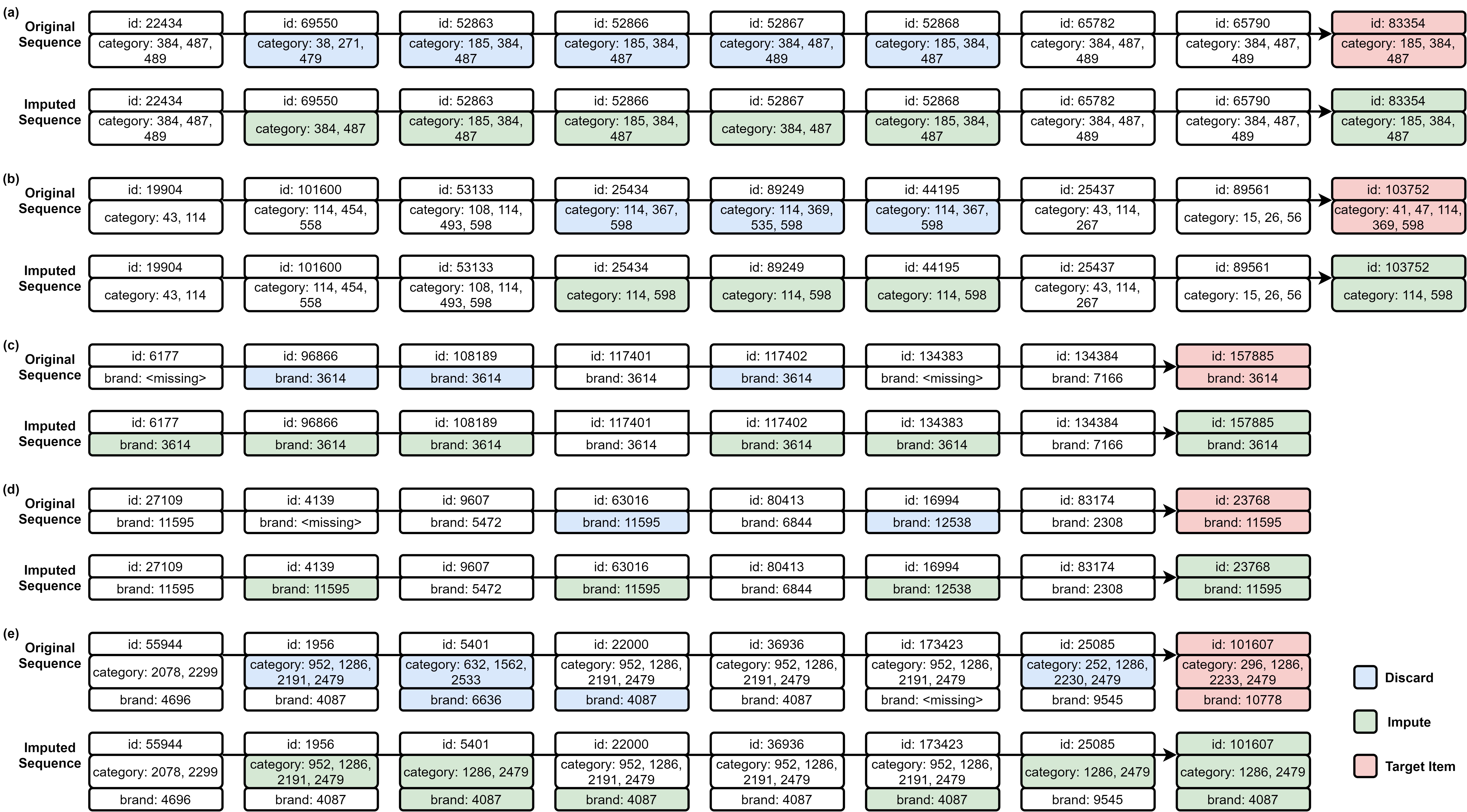
Figure 4. (a) and (b) are two sequences with their imputed categories from the “Beauty D” dataset, (c) and (d) are two sequences with their imputed brands from the “Toys and Games D” dataset, (e) is the sequence with its imputed categories and brands from the “Sports and Outdoors D” dataset.

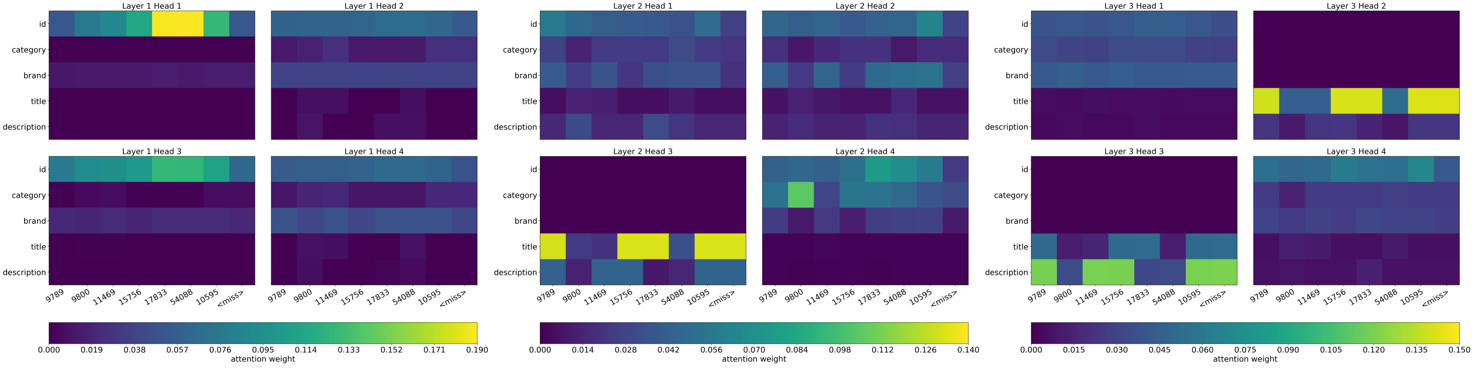
(a)

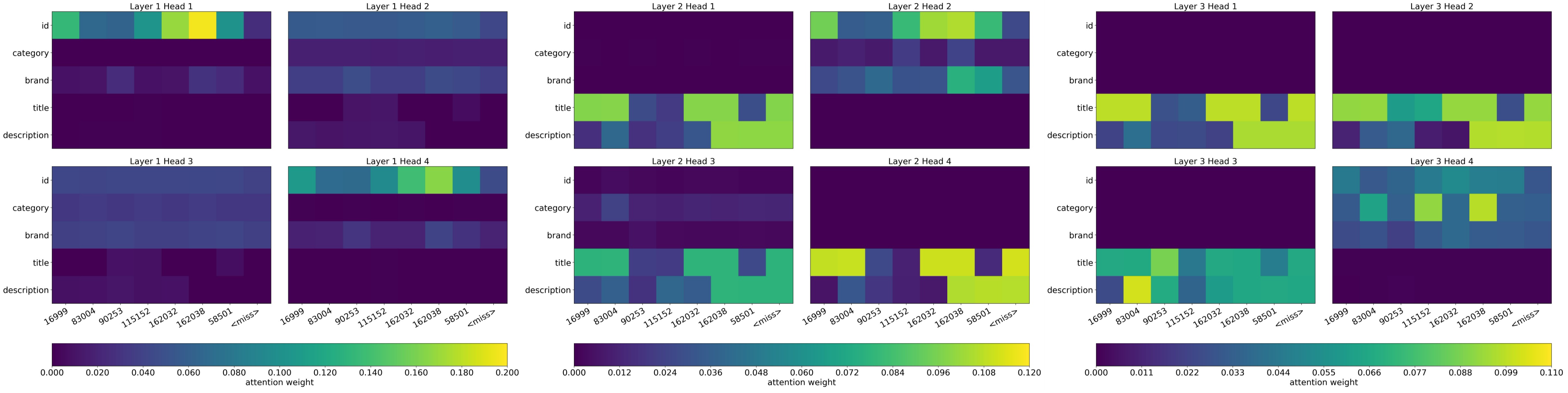
(b)

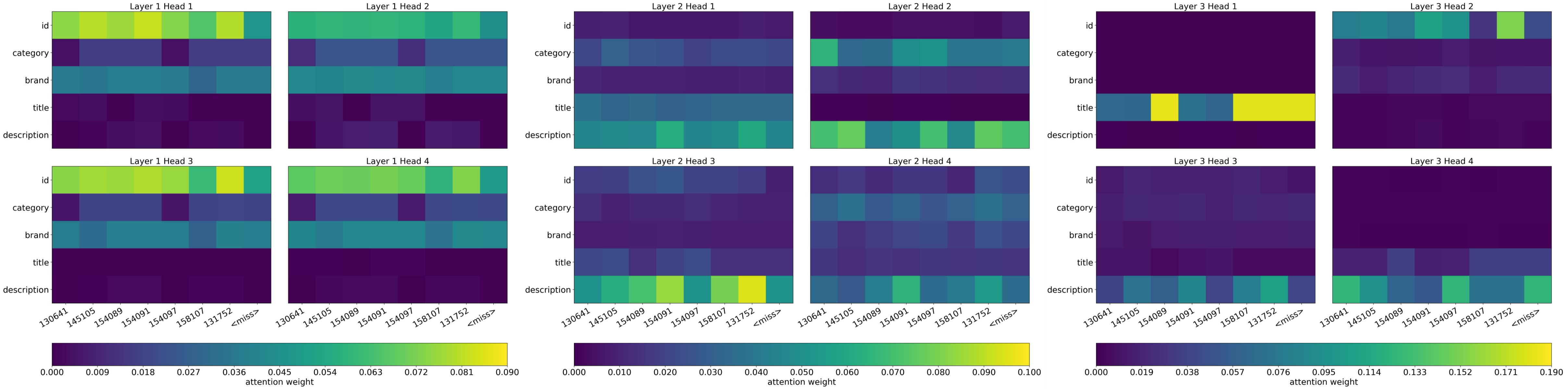
(c)

Figure 5. Visualization for the attention weights from the missing item ID field to all feature fields of all heads and layers in MIIR on three sequences from different datasets.

In Fig. 4 we list some sequences with their imputed results. We observe that MIIR generates different feature values for missing feature fields according to different contexts (i.e., items and sequences), which is better than using fixed predefined values. Moreover, MIIR is able to infer the ground-truth missing values, including the side information of the next item, to give the model with a more accurate guidance for recommendation. For example, MIIR imputes a part of the discarded categories in sequence (b) and the discarded brands in sequence (d). We can also observe that the side information of items in the same sequence may be related, which is why MIIR can infer the ground-truth missing values in light of the given context. However, MIIR tends to be over-dependent on the information from the sequence, leading it to impute inaccurate results. For instance, in sequence (e), MIIR imputes the wrong categories and brand for item 5401.

Additionally, we visualize the attention weights from the missing item ID (i.e., the next item ID) to all feature fields in the given sequence in DFSA, as shown in Fig. 5. We reshape the attention weights into a matrix of dimensions $5\times{n}$, where $5$ is the number of the feature field types and $n$ is the sequence length. First, we see that MIIR exploits the information from all feature fields of the given sequence to predict the next item, which emphasizes the necessity to model the relation between any pair of feature fields. Second, we observe that different layers focus on different types of feature fields, where the first layer mainly attends to ID, and the third layer mainly attends to title and description. This illustrates that MIIR gradually fuses different types of side information into the model by different layers. Because the information in textual feature fields is more difficult to extract, MIIR needs more deeper layers to fuse textual feature fields. Third, we find that different heads in the same layers have similar attention patterns, which means that there might be some redundant parameters in MIIR.

6. Conclusion

We have studied the missing side information problem in sequential recommendation. We have proposed the missing information imputation (MII) task to unify the missing side information imputation task and the sequential recommendation task. We have presented a novel sequential recommendation model named missing information imputation recommender (MIIR) to simultaneously impute missing feature values and predict the next item for a given sequence of items. We have proposed a dense fusion self-attention (DFSA) mechanism to model different relations in the item sequence and to fuse side information.

Based on experiments and analyses on three datasets with different settings of the missing rates we have found that MIIR outperforms state-of-the-art methods for sequential recommendation with side information. We have verified that MIIR can identify useful side information from missing feature fields by training with the MII task, and that the DFSA mechanism improves the recommendation effectiveness of MIIR.

As to broader implications of our work, we offer a new perspective by revealing a correlation between missing side information imputation and the sequential recommendation task. They both concern the prediction of missing information. The perspective operationalized with MIIR can be adopted as a foundational paradigm. Other prediction tasks related to recommendation, such as rating prediction, user profile prediction, and next basket recommendation can also be formulated as a MII task.

Limitations of our work are two-fold. (i) Since DFSA treats side information as part of the sequence (e.g., in our case, the actual sequence length is 5x the number of items) and models all possible pairwise relations in an item sequence, it is computationally costly and not easy to scale to long sequences; and (ii) we have not optimized the MII losses on different types of feature fields in MIIR for the recommendation task.

We aim to further improve MIIR in different directions. We will assess the ability of the linear transformer (Wang et al., 2020b; Xiong et al., 2021) to reduce the computational costs of DFSA and design a mechanism to filter out useless relations at an early stage. We also plan to design a tailored loss for MIIR by building on recent loss weighting methods (Du et al., 2018; Xu et al., 2019).

- (1)
- Ba et al. (2016) Jimmy Lei Ba, Jamie Ryan Kiros, and Geoffrey E Hinton. 2016. Layer normalization. arXiv preprint arXiv:1607.06450 (2016).
- Beaulieu-Jones and Moore (2017) Brett K Beaulieu-Jones and Jason H Moore. 2017. Missing data imputation in the electronic health record using deeply learned autoencoders. In Pacific Symposium on Biocomputing. 207–218.
- Biessmann et al. (2018) Felix Biessmann, David Salinas, Sebastian Schelter, Philipp Schmidt, and Dustin Lange. 2018. “Deep” learning for missing value imputation in tables with non-numerical data. In Conference on Information and Knowledge Management. 2017–2025.
- Binder et al. (2016) Alexander Binder, Sebastian Bach, Grégoire Montavon, Klaus-Robert Müller, and Wojciech Samek. 2016. Layer-wise relevance propagation for deep neural network architectures. International Conference on Information Science and Applications (2016), 913–922.
- Cai et al. (2021) Renqin Cai, Jibang Wu, Aidan San, Chong Wang, and Hongning Wang. 2021. Category-aware collaborative sequential recommendation. In International ACM SIGIR Conference on Research and Development in Information Retrieval. 388–397.
- Cao et al. (2019) Yixin Cao, Xiang Wang, Xiangnan He, Zikun Hu, and Tat-Seng Chua. 2019. Unifying knowledge graph learning and recommendation: Towards a better understanding of user preferences. In The Web Conference. 151–161.
- de Souza Pereira Moreira et al. (2021) Gabriel de Souza Pereira Moreira, Sara Rabhi, Jeong Min Lee, Ronay Ak, and Even Oldridge. 2021. Transformers4Rec: Bridging the gap between NLP and sequential/session-based recommendation. In ACM Conference on Recommender Systems. 143–153.
- Devlin et al. (2019) Jacob Devlin, Ming-Wei Chang, Kenton Lee, and Kristina Toutanova. 2019. BERT: Pre-training of deep bidirectional transformers for language understanding. In Proceedings of the Conference of the North American Chapter of the Association for Computational Linguistics. 4171–4186.
- Du et al. (2018) Yunshu Du, Wojciech M Czarnecki, Siddhant M Jayakumar, Mehrdad Farajtabar, Razvan Pascanu, and Balaji Lakshminarayanan. 2018. Adapting auxiliary losses using gradient similarity. arXiv preprint arXiv:1812.02224 (2018).
- Fang et al. (2020) Hui Fang, Danning Zhang, Yiheng Shu, and Guibing Guo. 2020. Deep learning for sequential recommendation: Algorithms, influential factors, and evaluations. ACM Transactions on Information Systems 39, 1 (2020), 1–42.
- Glorot and Bengio (2010) Xavier Glorot and Yoshua Bengio. 2010. Understanding the difficulty of training deep feedforward neural networks. In Proceedings of the International Conference on Artificial Intelligence and Statistics. 249–256.
- Hendrycks and Gimpel (2016) Dan Hendrycks and Kevin Gimpel. 2016. Gaussian error linear units (GELUs). arXiv preprint arXiv:1606.08415 (2016).
- Hernández-Lobato et al. (2014) José Miguel Hernández-Lobato, Neil Houlsby, and Zoubin Ghahramani. 2014. Probabilistic matrix factorization with non-random missing data. In International Conference on Machine Learning. 1512–1520.
- Hidasi and Karatzoglou (2018) Balázs Hidasi and Alexandros Karatzoglou. 2018. Recurrent neural networks with top-k gains for session-based recommendations. In Conference on Information and Knowledge Management. 843–852.
- Hidasi et al. (2016a) Balázs Hidasi, Alexandros Karatzoglou, Linas Baltrunas, and Domonkos Tikk. 2016a. Session-based recommendations with recurrent neural networks. In International Conference on Learning Representations.
- Hidasi et al. (2016b) Balázs Hidasi, Massimo Quadrana, Alexandros Karatzoglou, and Domonkos Tikk. 2016b. Parallel recurrent neural network architectures for feature-rich session-based recommendations. In ACM Conference on Recommender Systems. 241–248.
- Huang et al. (2018) Xiaowen Huang, Shengsheng Qian, Quan Fang, Jitao Sang, and Changsheng Xu. 2018. CSAN: Contextual self-attention network for user sequential recommendation. In Proceedings of the ACM International Conference on Multimedia. 447–455.
- Kang and McAuley (2018) Wang-Cheng Kang and Julian McAuley. 2018. Self-attentive sequential recommendation. In IEEE International Conference on Data Mining. 197–206.
- Kingma and Ba (2015) Diederik P Kingma and Jimmy Ba. 2015. Adam: A method for stochastic optimization. In International Conference on Learning Representations.
- Kipf and Welling (2017) Thomas N. Kipf and Max Welling. 2017. Semi-supervised classification with graph convolutional networks. In International Conference on Learning Representations.
- Lee et al. (2018) Youngnam Lee, Sang-Wook Kim, Sunju Park, and Xing Xie. 2018. How to impute missing ratings? Claims, solution, and its application to collaborative filtering. In The Web Conference. 783–792.
- Li et al. (2017) Jing Li, Pengjie Ren, Zhumin Chen, Zhaochun Ren, Tao Lian, and Jun Ma. 2017. Neural attentive session-based recommendation. In Conference on Information and Knowledge Management. 1419–1428.
- Lipton et al. (2015) Zachary C Lipton, John Berkowitz, and Charles Elkan. 2015. A critical review of recurrent neural networks for sequence learning. arXiv preprint arXiv:1506.00019 (2015).
- Liu et al. (2021) Chang Liu, Xiaoguang Li, Guohao Cai, Zhenhua Dong, Hong Zhu, and Lifeng Shang. 2021. Non-invasive self-attention for side information fusion in sequential recommendation. In Proceedings of the AAAI Conference on Artificial Intelligence, Vol. 35. 4249–4256.
- Marlin and Zemel (2009) Benjamin M Marlin and Richard S Zemel. 2009. Collaborative prediction and ranking with non-random missing data. In ACM Conference on Recommender Systems. 5–12.
- Ni et al. (2019) Jianmo Ni, Jiacheng Li, and Julian McAuley. 2019. Justifying recommendations using distantly-labeled reviews and fine-grained aspects. In Proceedings of the Conference on Empirical Methods in Natural Language Processing. 188–197.
- Pan et al. (2015) Ruilin Pan, Tingsheng Yang, Jianhua Cao, Ke Lu, and Zhanchao Zhang. 2015. Missing data imputation by K nearest neighbours based on grey relational structure and mutual information. Applied Intelligence 43, 3 (2015), 614–632.
- Pascanu et al. (2013) Razvan Pascanu, Tomas Mikolov, and Yoshua Bengio. 2013. On the difficulty of training recurrent neural networks. In International Conference on Machine Learning. 1310–1318.
- Pereira et al. (2020) Ricardo Cardoso Pereira, Miriam Seoane Santos, Pedro Pereira Rodrigues, and Pedro Henriques Abreu. 2020. Reviewing autoencoders for missing data imputation: Technical trends, applications and outcomes. Journal of Artificial Intelligence Research 69 (2020), 1255–1285.
- Rendle et al. (2009) Steffen Rendle, Christoph Freudenthaler, Zeno Gantner, and Lars Schmidt-Thieme. 2009. BPR: Bayesian personalized ranking from implicit feedback. In Proceedings of the Conference on Uncertainty in Artificial Intelligence. 452–461.
- Shi et al. (2019) Shaoyun Shi, Min Zhang, Xinxing Yu, Yongfeng Zhang, Bin Hao, Yiqun Liu, and Shaoping Ma. 2019. Adaptive feature sampling for recommendation with missing content feature values. In Conference on Information and Knowledge Management. 1451–1460.
- Singer et al. (2022) Uriel Singer, Haggai Roitman, Yotam Eshel, Alexander Nus, Ido Guy, Or Levi, Idan Hasson, and Eliyahu Kiperwasser. 2022. Sequential modeling with multiple attributes for watchlist recommendation in e-commerce. In International Conference on Web Search and Data Mining. 937–946.
- Srivastava et al. (2014) Nitish Srivastava, Geoffrey Hinton, Alex Krizhevsky, Ilya Sutskever, and Ruslan Salakhutdinov. 2014. Dropout: A simple way to prevent neural networks from overfitting. The Journal of Machine Learning Research 15, 1 (2014), 1929–1958.
- Sun et al. (2019) Fei Sun, Jun Liu, Jian Wu, Changhua Pei, Xiao Lin, Wenwu Ou, and Peng Jiang. 2019. BERT4Rec: Sequential recommendation with bidirectional encoder representations from transformer. In Conference on Information and Knowledge Management. 1441–1450.
- Tang et al. (2018) Gongbo Tang, Mathias Müller, Annette Rios Gonzales, and Rico Sennrich. 2018. Why self-attention? A targeted evaluation of neural machine translation architectures. In Proceedings of the Conference on Empirical Methods in Natural Language Processing. 4263–4272.
- Tang and Wang (2018) Jiaxi Tang and Ke Wang. 2018. Personalized top-n sequential recommendation via convolutional sequence embedding. In International Conference on Web Search and Data Mining. 565–573.
- Vaswani et al. (2017) Ashish Vaswani, Noam Shazeer, Niki Parmar, Jakob Uszkoreit, Llion Jones, Aidan N Gomez, Łukasz Kaiser, and Illia Polosukhin. 2017. Attention is all you need. In Neural Information Processing Systems, Vol. 30.
- Wang et al. (2018) Cheng Wang, Mathias Niepert, and Hui Li. 2018. LRMM: Learning to recommend with missing modalities. In Proceedings of the Conference on Empirical Methods in Natural Language Processing. 3360–3370.
- Wang et al. (2020a) Pengfei Wang, Yu Fan, Long Xia, Wayne Xin Zhao, ShaoZhang Niu, and Jimmy Huang. 2020a. KERL: A knowledge-guided reinforcement learning model for sequential recommendation. In International ACM SIGIR Conference on Research and Development in Information Retrieval. 209–218.
- Wang et al. (2020b) Sinong Wang, Belinda Z Li, Madian Khabsa, Han Fang, and Hao Ma. 2020b. Linformer: Self-attention with linear complexity. arXiv preprint arXiv:2006.04768 (2020).
- Wu et al. (2020) Le Wu, Yonghui Yang, Kun Zhang, Richang Hong, Yanjie Fu, and Meng Wang. 2020. Joint item recommendation and attribute inference: An adaptive graph convolutional network approach. In International ACM SIGIR Conference on Research and Development in Information Retrieval. 679–688.
- Wu et al. (2019) Shu Wu, Yuyuan Tang, Yanqiao Zhu, Liang Wang, Xing Xie, and Tieniu Tan. 2019. Session-based recommendation with graph neural networks. In Proceedings of the AAAI Conference on Artificial Intelligence, Vol. 33. 346–353.
- Xie et al. (2022) Yueqi Xie, Peilin Zhou, and Sunghun Kim. 2022. Decoupled side information fusion for sequential recommendation. In International ACM SIGIR Conference on Research and Development in Information Retrieval.
- Xiong et al. (2021) Yunyang Xiong, Zhanpeng Zeng, Rudrasis Chakraborty, Mingxing Tan, Glenn Fung, Yin Li, and Vikas Singh. 2021. Nyströmformer: A nyström-based algorithm for approximating self-attention. In Proceedings of the AAAI Conference on Artificial Intelligence, Vol. 35. 14138–14148.
- Xu et al. (2019) Yichong Xu, Xiaodong Liu, Yelong Shen, Jingjing Liu, and Jianfeng Gao. 2019. Multi-task learning with sample re-weighting for machine reading comprehension. In Proceedings of the Conference of the North American Chapter of the Association for Computational Linguistics. 2644–2655.
- Yuan et al. (2021) Xu Yuan, Dongsheng Duan, Lingling Tong, Lei Shi, and Cheng Zhang. 2021. ICAI-SR: Item categorical attribute integrated sequential recommendation. In International ACM SIGIR Conference on Research and Development in Information Retrieval. 1687–1691.
- Zeng et al. (2021) Zheni Zeng, Chaojun Xiao, Yuan Yao, Ruobing Xie, Zhiyuan Liu, Fen Lin, Leyu Lin, and Maosong Sun. 2021. Knowledge transfer via pre-training for recommendation: A review and prospect. Frontiers in Big Data (2021), 4.
- Zhang et al. (2019) Tingting Zhang, Pengpeng Zhao, Yanchi Liu, Victor S Sheng, Jiajie Xu, Deqing Wang, Guanfeng Liu, and Xiaofang Zhou. 2019. Feature-level deeper self-attention network for sequential recommendation.. In International Joint Conference on Artificial Intelligence. 4320–4326.
- Zhao et al. (2020) Hengshuang Zhao, Jiaya Jia, and Vladlen Koltun. 2020. Exploring self-attention for image recognition. In Proceedings of the IEEE/CVF Conference on Computer Vision and Pattern Recognition. 10076–10085.
- Zhou et al. (2020) Kun Zhou, Hui Wang, Wayne Xin Zhao, Yutao Zhu, Sirui Wang, Fuzheng Zhang, Zhongyuan Wang, and Ji-Rong Wen. 2020. S3-rec: Self-supervised learning for sequential recommendation with mutual information maximization. In Conference on Information and Knowledge Management. 1893–1902.